Geophys. J. Int. (2007) 169, 821–829 doi: 10.1111/j.1365-246X.2007.03330.x

GJI

Geo

desy

,pot

ential

fiel

dan

dap

plie

dge

ophy

sics

Estimation of the pole tide gravimetric factor at the chandler periodthrough wavelet filtering

X.-G. Hu,1 L.-T. Liu,1 B. Ducarme,2 H. J. Xu1 and H.-P. Sun1

1Institute of Geodesy and Geophysics, Chinese Academy of Sciences, 340 Xu-Dong Road, Wuhan, China. E-mail: hxg432@sohu.com2Research Associate NFSR, Royal Observatory of Belgium, Av. Circulaire 3, B-1180, Brussels, Belgium

Accepted 2006 December 12. Received 2006 October 13; in original form 2006 February 9

S U M M A R YWavelet analysis for filtering is used to improve estimation of gravity variations induced byChandler wobble. This method eliminate noise in superconducting gravimeter (SG) recordswith bandpass filters derived from Daubechies wavelet. The SG records at four Europeanstations (Brussels, Membach, Strasbourg and Vienna) are analysed in this study. First, the earthtidal constituents are removed from the observed data by using synthetic tides, then the gravityresiduals are filtered into a narrow period band of 256–512 d by a wavelet bandpass filter. Thesedata are submitted to three regression analysis methods for estimating the gravimetric factor ofthe Chandler wobble. After processing by wavelet filtering, SG records can provide amplitudefactors δ and phase lags κ of the Chandler wobble with much smaller mean square deviation(MSD) than these provided by former studies. It is mainly because the wavelet method caneffectively eliminate instrumental drift and provide smoothed data series for the regressionanalysis.

Key words: Chandler wobble, pressure correction, superconducting gravimeter, waveletfilter.

1 I N T RO D U C T I O N

Variations in the geocentric position of the rotation axis (i.e. po-

lar motion) of the earth will perturb the centrifugal force and thus

deform the Earth. Polar motion consists of two main frequency com-

ponents: the Chandler wobble and the forced annual wobble at period

about 432 and 365 d, respectively. Modern space geodetic observa-

tion techniques, such as very long baseline interferometer (VLBI)

and global positioning system (GPS), can now observe the temporal

variations of earth orientation parameters (EOP) with an accuracy

less than 1 mas (1 mas = 1 milli-arcsecond). The time-dependent

Earth deformation induced by the Polar motion can affect high-

precise gravity observations. The superconducting gravimeter (SG)

is the world’s most sensitive and stable gravimeter. With a sensitivity

of 0.01 nm s−2 and instrument drift less than a few 10 nm s−2 per

year, the SG is able to observe gravity effects caused by the polar

motion, the so-called ‘pole tide’. The pioneering work of study of

the polar motion using SG records goes back to Richter & Zurn

(1988). After them some challenging studies to investigate the na-

ture of the gravity variations caused by the polar motion using SG

and EOP data have been conducted (De Meyer & Ducarme 1991;

Richter et al. 1995; Sato et al. 1997; Loyer et al. 1999; Sato et al.2001; Xu et al. 2004; Harnisch & Harnisch 2006).

However, all the above mentioned previous works brings out sev-

eral points worthy of further consideration. First, the instrumental

drift is usually approximated by polynomial or exponential model

over the entire observation intervals. Such an approximation is ef-

fective when the drift is continuous but it certainly fails when SG

measurement has jumps or discontinuities, the observation from SG

T003 at the station Brussels is such a case (Ducarme et al. 2005).

Secondly, Because of no efficient narrow bandpass filter in previ-

ous works, the annual and Chandler components in SG records are

usually filtered into a comparatively wide frequency band in which

there still exist large, complicated long-period regional perturba-

tions which can be hardly removed by mathematical models and may

affect the estimation of the gravimetric factors of the pole tide. Fur-

thermore, some previous studies used the same atmospheric pressure

correction in the pole tide analysis as in the Earth tidal analysis at

daily and subdaily period, that is, correction with a mean baromet-

ric admittance over whole frequency range. However many studies

proved that the admittance was obviously frequency-dependent and

that its value at low frequency was significantly smaller than the

mean value (e.g. Crossley et al. 1995; Neumeyer 1995; Hu et al.2005, 2006b). The gravity residuals in the pole tide band could thus

be overcorrected if a mean local barometric admittance is used in

the pressure correction.

The main motivation behind this study is to try to solve the prob-

lems quoted above with wavelet filtering method.

In the following Section 2, we simply introduce the rationale

of the wavelet filtering method. In Section 3, SG records from four

European stations are processed to obtain gravity residuals, and the-

oretical pole tides are computed from IERS data. Then in Section 4,

the wavelet filtering is applied on gravity residuals to eliminate in-

strumental drift and other noise. Section 5 estimates the gravimetric

C© 2007 The Authors 821Journal compilation C© 2007 RAS

822 X.-G. Hu et al.

factor of pole tide at Chandler frequency by using three regres-

sion analysis methods. Finally, the results of different methods and

authors are compared and discussed in Section 6, together with ad-

ditional considerations on the pressure correction.

2 WAV E L E T F I LT E R I N G M E T H O D

It is well known that a Fourier analysis expands a signal f (t) in

terms of sines and cosines. The signal can also be decomposed

into a weighted sum of different wavelets derived from dilation and

translation of two closely related basic functions, scaling function

φ(t) and analysing wavelet ψ(t)

f (t) =∑

n

aJ (n) 2J/2φ(2J t − n) +J∑

j=1

∑n=0

d j (n) 2 j/2ψ(2 j t − n),

(1)

where J , j and n are integer indices. The dilation 2 j allows the

characterization of the frequency contents of the signal while the

translation n enables the localization of different frequency content

in time–space (e.g. Mallat 1989a,b; Daubechies 1992). Decompo-

sition coefficients d j (n) are known as the dyadic discrete wavelet

transform of the signal and they reflect high frequency variations of

the signal, and coefficients a J (n) are approximation coefficients of

the signal at scale 2−J and they reflect low frequency variations

of the signal. These decomposition coefficients are implemented

efficiently using a pyramid algorithm, a remarkably fast algorithm

that involves low- and high-pass filtering along with a downsam-

pling (decimation) or up-sampling (zero-padding) operator (Mallat

1989a).

With different scale index J , a J (n) and d j (n) are different. So

eq. (1) is the multiresolution decomposition that represents char-

acteristics of the signal at different resolutions (Mallat 1989b). In

wavelet decomposition, each scale index j roughly corresponds to a

period band:

[2 j�t, 2 j+1�t], j = 1, 2, . . . , J, (2)

where �t is the sampling interval of the signal. Thus, wavelet trans-

form is actually parallel bandpass filtering. We can select appropriate

wavelet to make the wavelet filter adapt to the signal to get better

filtering performance. The Daubechies wavelet (Daubechies 1988)

is effective for extracting harmonics in signals because it is a com-

pact support (i.e. non-zero only over a finite-region) and orthogonal

wavelet.

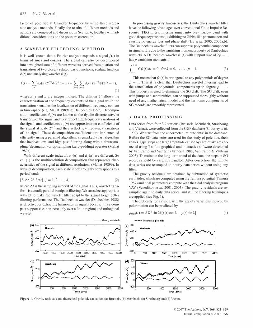
Figure 1. Gravity residuals and theoretical pole tides at station (a) Brussels, (b) Membach, (c) Strasbourg and (d) Vienna.

In processing gravity time-series, the Daubechies wavelet filter

have the following advantages over conventional Finite Impulse Re-

sponse (FIR) filters: filtering signal into very narrow band with

good frequency response, exhibiting no Gibbs-like phenomenon and

causing no energy loss and phase shift (Hu et al. 2005, 2006a,b).

The Daubechies wavelet filters can suppress polynomial component

in signals. It is due to the vanishing moment property of Daubechies

wavelets. A Daubechies wavelet ψ (t) with support size of 2p − 1

has p vanishing moments if∫ +∞

−∞t kψ(t) dt = 0, for k = 0, 1, . . . , p − 1. (3)

This means that ψ (t) is orthogonal to any polynomials of degree

p − 1. Thus it is clear that Daubechies wavelet filtering lead to

the cancellation of polynomial components up to degree p − 1.

This property is used to eliminate the SG drift. The SG drift, even

with jumps or discontinuities, can be suppressed thoroughly without

need of any mathematical model and the harmonic components of

SG records are smoothly represented.

3 DATA P RO C E S S I N G

Data series from four SG stations (Brussels, Membach, Strasbourg

and Vienna), were collected from the GGP database (Crossley et al.1999). We start from the uncorrected ‘minute data’ in the database.

Before the SG data series are used for the study of pole tide, their

spikes, gaps, steps and large amplitude caused by earthquake are cor-

rected using T-soft; a graphical and interactive software developed

by Van Camp and Vauterin (Vauterin 1988; Van Camp & Vauterin

2005). To maintain the long-term trend of the data, the steps in SG

records should be carefully handled. After correction, the minute

data series are resampled to hourly data series without using any

filter.

The gravity residuals are obtained by subtraction of synthetic

earth tides, which are computed using the Tamura potential (Tamura

1987) and tidal parameters compute with the tidal analysis program

VAV (Venedikov et al. 2001, 2003). The gravity residuals are re-

sampled again to daily data series, and still no filtering techniques

are applied (see Fig. 1).

Theoretically for a rigid Earth, the gravity variations induced by

polar motion can be predicted by

prigid(t) = R�2 sin 2θ [x(t) cos λ + y(t) sin λ] (4)

C© 2007 The Authors, GJI, 169, 821–829

Journal compilation C© 2007 RAS

Estimation of the pole tide gravimetric factor 823

(e.g. Kaneko et al. 1974; Wahr 1985; Capitaine 1986; Hinderer &

Legros 1989), where R(6.371 × 106 m) is the mean geocentric ra-

dius, �(7.292115 × 10−5 rad s−1) is the mean angular velocity of

the Earth, and θ and λ are the colatitude and west longitude of the

observation site, respectively. x(t) and y(t), expressed in arcseconds,

are the instantaneous pole coordinates in the Celestial Ephemeris

Pole relative to the International Reference Pole. Here we use polar

motion data set EOPC04 and eq. (4) to determine theoretical pole

tides at SG stations. EOPC04 is a smoothed EOP data set provided

by IERS (International Earth Rotation Service), derived on a one-

day basis, at midnight (00.00 hr UTC), from VLBI, Lunar Laser

Ranging (LLR), Satellite Laser Ranging (SLR) and GPS measure-

ments. Theoretical pole tides at the four SG stations are shown in

Fig. 1.

4 WAV E L E T F I LT E R I N G O F G R AV I T Y

R E S I D UA L S

The upward trend of gravity residuals in Fig. 1 comes from the in-

strumental drift of SG and some real long-term gravity variations.

Usually in tidal gravity analysis the instrumental drift of SG is de-

scribed by polynomials, such as linear or quadratic drift model.

When the SG data series covers several years, a simple mathemat-

ical function sometimes is not sufficient because the SG drift can

hardly remain a perfectly continuous function (without jump and

rapid behaviour changes). The SG measurement at station Brussels

is a typical case.

In order to eliminate the instrumental drift, we filter gravity resid-

uals into a very narrow subband 1/28 ∼ 1/27 cpd, that is, period 256

to 512 d, by using a Daubechies wavelet filter. Thus noise outside

this band is removed, including instrument drift and high frequency

noise. The same is done with the set of theoretical gravity data,

derived from the observed polar motion and eq. (4). The local baro-

metric measurements are also filtered in the same way in order to

estimate atmospheric effects in the pole tidal band.

After subtraction of the instrumental drift, the remaining residues

oscillate around the zero line. This signal is mainly caused by the

superposition of the influence of the annual and Chandler wobble.

Fig. 2 shows that the observed pole tide corresponds quite well to

the theoretical pole tide at the station Membach, Strasbourg and

Vienna, which means the gravity effect of the polar motion is nearly

Figure 2. Wavelet filtering results for data series at station (a) Brussels, (b) Membach, (c) Strasbourg and (d) Vienna.

completely represented by the recorded gravity. The station Brussels

is an exception due to its extra large annual noise (see Fig. 3).

To check cleaning capabilities of the wavelet method, we com-

pare the filtered gravity residuals with unfiltered ones at the four

stations in the frequency domain. The spectra in Fig. 3 show that

long-period components are clearly removed after wavelet filtering

but the polar motion signal is unaffected. We can also see from

Fig. 3 that there are large annual signal at the stations Brussels

and Strasbourg. In Strasbourg and Vienna the annual component

is not separable. Besides the annual wobble effect, the anomalous

annual signal could be due to the global annual variations in the

sea level, atmosphere, hydrology cycle and other annual geophys-

ical effects, but until now most of these effects have not yet been

accurately modelled. Moreover, the instrumental reactions to mete-

orological effects are very complex and could trigger large annual

variations in the measurement, such as the effect of annual tem-

perature variation of the room where the SG is located and the

effect of annual tilt variation (the Brussels instrument was not tilt

compensated).

5 R E G R E S S I O N A N A LY S I S

To estimate the amplitude factor δ and phase difference κ of Chan-

dler wobble, we have to separate the chandler constituent from the

annual one. In the following, three separation methods are described.

The measurement from the station Membach is taken as an example

to give some detail demonstration.

5.1 Fitting sinusoidal functions to the pole tide

Least-squares fitting of two sinusoidal functions with period 432

and 365.25 d to the pole tide in the time domain is a usual method

to separate the Chandler component from the annual one (e.g. Xu

et al. 2004; Harnisch & Harnisch 2006).

After wavelet filtering of SG data, the regression adjustment be-

comes quite easy as not much environmental noise is left in the

period band 256–512 d. The data series in the period band 256–

512 d can be simply modelled as sum of two sinusoidal functions

�g1(t) =2∑

i=1

Ai cos(ωi t + ai ) + C · P(t, �T ), (5)

C© 2007 The Authors, GJI, 169, 821–829

Journal compilation C© 2007 RAS

824 X.-G. Hu et al.

Figure 3. Comparison between the filtered and unfiltered gravity residuals in the frequency domain at station (a) Brussels, (b) Membach, (c) Strasbourg and

(d) Vienna. The passband of the filter is 0.713 ∼ 1.42 6 cpy (period band 256 ∼ 512 d). These time-series are padded with zeros at their ends to length 65 536

and then multiply by Hanning windows before performing fast Fourier transform (FFT) to them.

while index i = 1, 2 stands for the Chandler and annual component,

respectively, P(t , �T ) is the local atmospheric pressure signal in

the period range �T = 256 ∼ 512 d, and C represents a value of

barometric admittance, which is frequency-dependent.

Similarly the theoretical pole tide derived from eq. (4) is modelled

as

�g2(t) =2∑

i=1

Bi cos(ωi t + bi ). (6)

We fit �g1 to the observed pole tide �G(t) (filtered gravity resid-

ual) and �g2 to theoretical pole tide �p (derived from eq. 4) by

using the least-squares technique. After adjustment of the parame-

ters Ai , Bi , ai and bi , amplitude factor δ and phase difference κ at

Chandler period can be estimated as:

δ = A1/B1, κ = a1 − b1. (7)

Because in eq. (4) the observed polar motion is variable and θ

and λ are different at different stations, the Chandler frequency is

not a constant for different stations and different epochs. In order

to obtain the best fitting result, we select an optimum Chandler

frequency by experimenting different ω1 from 428 to 438 d step by

0.5 d until we find a minimum root mean squared (rms) value of

the difference between the model �p and the theoretical pole tide.

The optimum value, for example, at the station Membach is 431 d,

and the corresponding minimum rms is about 2.1 nms−2. Fig. 4

shows a good agreement between the sinusoidal functions and the

pole tide at the station Membach. The value δ and κ are 1.1960 ±0.0119 and 0.6847 ± 0.9126, respectively. The fitting results of

the station Membach and of the three other stations are listed in

Table 1.

5.2 Direct fit in the time domain

Because the Chandler wobble is not a pure harmonic, Chandler

frequency is not a single value but a set of close frequencies. To

avoid using a fixed Chandler frequency in the regression analysis,

we try to fit directly the theoretical pole tide to SG records in the

time domain. Since the Earth response to the long-period tide is

not strongly frequency dependent, we may accept that amplitude

factor δ at the Chandler period is equal to that at annual period.

For simplicity of model derivation, we mix up the annual terms

of all different origin, except for annual wobble, in one sinusoidal

expression (Ducarme et al. 2006), then the observed pole tide �G(t)in the period band 256–512 d can be modelled as

�g(t) = δ�p(t − �t) + A cos(ωt + b) + C · P(t, �T ), (8)

C© 2007 The Authors, GJI, 169, 821–829

Journal compilation C© 2007 RAS

Estimation of the pole tide gravimetric factor 825

Figure 4. Fitting sinusoidal functions to the pole tide at the station Membach. (a) The best fit for the observed pole tide. (b) The best fit for the theoretical pole

tide. The period band is 256 ∼512 d and the length of the time-series is 3676 d.

Table 1. Results from different methods, δ: Amplitude factor, κ (◦): Phase difference (lag positive), Admittance in nms−2 hPa−1, mean

value: pressure admittance determined in the diurnal and semi-diurnal bands.

Station Method δ κ (◦) Pressure

admittance

Brussels (a) This study (13, Apr. 04, 1987 ∼ 25, May 05, 2000)

Sinusoidal fit (435 d) 1.1820 ± 0.0338 −0.5967 ± 2.0926 2.84

Fitting in the time domain 1.1713 ± 0.0067 about −2.52

Fitting in the frequency domain 1.1939 ± 0.0294 −2.4088 ± 1.4133

(b) Previous studiesXu et al. (2004)b 1.1848 ± 0.0504 −6.36 ± 2.43 2.81

Harnisch & Harnisch (2006)b 1.18 ± 0.26 −8.3 ± 11.0 Mean value

Ducarme et al. (2006)a 1.1865 ± 0.0126 about −2.52

Membach (a) This study (24,Aug, 1995 ∼ 15,Sep.,2005)

Sinusoidal fit (431 d) 1.1960 ± 0.0119 0.6487 ± 0.9126 −2.61

Fitting in the time domain 1.1896 ± 0.0084 about 0.83

Fitting in the frequency domain 1.2739 ± 0.0019 0.6612 ± 0.0848

(b) Previous studiesXu et al. (2004)b 1.2613 ± 0.0187 −4.97 ± 0.85 −2.35

Harnisch & Harnisch (2006)b 1.18 ± 0.13 about 2.4 Mean value

Ducarme et al. (2006)a 1.1897 ± 0.0137 about 1.68

Strasbourg (a) This study(20,Apr., 1997 ∼ 03,Jun, 2005)

Sinusoidal fit (435.5 d) 1.1902 ± 0.0157 4.3190 ± 1.3261 −2.30

Fitting in the time domain 1.1910 ± 0.0030 about 4.15

(b) Previous studiesXu et al. (2004)b 1.1767 ± 0.0664 −27.04 ± 3.2 3 −3.76

Harnisch & Harnisch (2006)b 1.18 ± 0.14 about −0.5 Mean value

Ducarme et al. (2006)a 1.1856 ± 0.0148 about 1.68

Vienna (a) This study (21,Aug.,1997 ∼ 2,Oct.,2004)

Sinusoidal fit (432 d) 1.2092 ± 0.0127 −5.7917 ± 1.3345 −2.73

Fitting in the time domain 1.2280 ± 0.0082 about −4.98

(b) Previous studiesHarnisch & Harnisch (2006)b 1.20 ± 0.13 about 5.0 Mean value

Ducarme et al. (2006)a 1.1526 ± 0.0086 about −1.68

aFitting in the time domain.bFitting at a fixed Chandler period of 432 d.

where �p(t) is theoretical pole tide and �t is time lag between

the observed pole tide �G(t) and the theoretical pole tide �p(t).The second term in eq. (8) is the model of environmental noise at

annual frequency. The third term is the local atmospheric pressure

effects, just as in eq. (5). The amplitude factor δ, parameter A, b and

admittance C are estimated by fitting �G(t) to the filtered gravity

residual �G(t) with the least-square method at a optimum value

of �t . The optimum time lag �t is determined by experimenting

different values of �t in the process of adjustment of A, b, C and

δ until we find a minimum rms value of the difference between

�G(t) and �G(t). Using this model we do not have to know the

exact frequency of the Chandler wobble.

C© 2007 The Authors, GJI, 169, 821–829

Journal compilation C© 2007 RAS

826 X.-G. Hu et al.

Figure 5. (a) Determination of optimum time lag �t CH by selecting the minimum rms between observed pole tides and theoretical ones. (b) The result of

directly fitting theoretical tides to observed pole tides SG observations with time lag of a day. The period band is 256 ∼ 512 d and the length of the data is 3676 d.

Fig. 5 shows the fit with a lag �t CH of a day and an example of

determination of the optimum value for �t . At the optimum value

of one day shift, this method yields δ = 1.1896 ± 0.0084 at station

Membach. As the period of the Chandler wobble is around 432 d,

one day shift corresponds to a phase lag about 0.83◦. Compared to

the results derived from the sinusoidal fitting method, the amplitude

factor δ agrees within the mean square deviation (MSD) but the

precision is much improved (see Table 1).

5.3 Fit in the frequency domain

According to Fourier analysis theory, at least 6.5 yr long time-series

is necessary to separate the Chandler component from the annual one

in the frequency domain with a rectangular window. We can see from

Fig. 3 that with the Hanning window the spectrum peak at the annual

frequency is partly separated from that at the Chandler frequency

for data from Brussels and Membach. The rectangular window can

provide better resolution of gravity spectra if its spectral leakage is

suppressed. To reduce spectral leakage of in the Discrete Fourier

transform, we removed large long-period components by wavelet

Figure 6. Discrete Fourier transform of pole tides at the station Brussels (a) and Membach (b), now with rectangular window. Prior to FFT the data is padded

with zeros from 4792 (Brussels) and 3676 (Membach) to 65 536 points, and large long-term components are filtered out in order to reduce spectral leakage.

filtering before performing Fourier transform. Fig. 6 shows that two

peaks are almost totally separated by using rectangular windows.

After wavelet filtering gravity residuals, the spectral leakage of the

rectangular window is only a little bit larger than that of the Hanning-

window, but the resolution of spectrum is much improved (compare

it with Figs 3a and b).

We try to estimate the amplitude factor δ and phase difference κ

of Chandler wobble in the frequency domain. The gravimetric factor

is defined in the frequency domain as:

δ( f ) = G( f )

P( f ), (9)

where f represents frequency, G(f ) and P(f ) are the discrete Fourier

transform of the observed pole tides and of the theoretical pole

tides, respectively. Thus the factor δ( f ) is a complex scalar, namely,

δ( f ) = δe−iκ , where δ is amplitude factor and κ is phase difference

between G(f ) and P(f ). The linear regression transfer function is

performed as

�G( f ) = G( f ) − δ( f )P( f ). (10)

C© 2007 The Authors, GJI, 169, 821–829

Journal compilation C© 2007 RAS

Estimation of the pole tide gravimetric factor 827

Minimizing |�G( f )|2 in a least squares sense over a narrow fre-

quency range f = 1/440 ∼ 1/424 cpd lead to

δ( f ) =∑

[G( f )P( f )]∑ |P( f )|2 (11)

The real and imaginary solutions are

δR =∑

[G R( f )PR( f ) + G I ( f )PI ( f )]∑ |P( f )|2 (12)

δI =∑

[G I ( f )PR( f ) − G R( f )PI ( f )]∑ |P( f )|2 . (13)

These can be combined into the amplitude factor δ =√

δ2R + δ2

I

and phase difference κ = arctg(δ I /δ R). With a rectangular window,

we obtain δ = 1.1939 ± 0.0294, κ = −2.4088◦ ± 1.4133 at the sta-

tion Brussels and δ = 1.2739 ± 0.0019, κ = 0.6612◦ ± 0.0848 at the

station Membach. Note that it is the first time that Fourier transform

is used in pole tide analysis. The amplitude factors obtained in the

frequency domain are obviously larger than values we just obtained

in the time domain. It is mainly due to the fact that observed pole

tides at Brussels and Membach have some components which are

not included in theoretical pole tides.

Figure 7. Gravity variations before and after local pressure corrections (with admittances in Table 1). The barometric effect is the local barometric data

multiplied by a barometric admittance. The long-period term of gravity variation is eliminated by wavelet filtering. The Hanning-window is used before

performing FFT.

6 R E S U LT S A N D D I S C U S S I O N S

Wavelet filtering method based on Daubechies wavelet shows ad-

vantage in analysis of long-term gravity variations in gravimetric

time-series. Table 1 gives a summary of our results and a com-

parison with previous results from different authors. In most cases,

although the estimated δ-factors agree within their associated MSD,

it is clear that the rms errors derived from this study are significantly

smaller than those from previous studies, which means that our re-

sults are more reliable. Our estimation yields higher internal preci-

sion mainly because wavelet filtering method eliminates effectively

the instrumental drift and provides smoothed data series for the re-

gression analysis. As a matter of fact, the wavelet method removes

all constituents outside the period range 256–512 d, including not

only the instrumental drift but also real long-term constituents of

other origins. Absolute gravity measurements are no more required

to support the drift modelling.

The estimated κ-values of different methods are quite scattered in

Table 1. We infer that some unreasonable κ-values may be due to the

method itself. There is a reasonable agreement between Ducarme

et al. (2006) and this study.

It has been usually believed that at low frequency the local baro-

metric pressure cannot be used to adequately remove the long-period

C© 2007 The Authors, GJI, 169, 821–829

Journal compilation C© 2007 RAS

828 X.-G. Hu et al.

air pressure effect, as the pressure cells have a regional extension.

However, it is not really the case, Boy et al. (2002) showed that

the global 3-D atmospheric loading modelling allows a significant

reduction of gravity residuals versus the correction using local baro-

metric admittance. However, this reduction is effective only between

about 5 and 100 d. For longer periods, the global pressure correction

does not show better improvement than local pressure correction in

term of reduction of the variance of gravity residuals. It is a reason

why the local pressure correction is still used in this study for the

pole tide analysis.

Barometric admittance values (see Table 1), estimated in the pe-

riod band 256–512 d by least-squares adjustment in the ‘fitting-

in-the-time-domain method’, are obviously smaller than their cor-

responding mean values over the whole frequency band, that is,

about −3.467, −3.303, −3.02 and −3.532 nms−2 hPa−1 at the sta-

tion Brussels, Membach, Strasbourg and Vienna, respectively. Local

atmospheric pressure corrections with frequency-dependent admit-

tances can avoid injecting extra noise in the pole tide band.

Fig. 7 shows spectra of surface gravity variations for four sta-

tions before any atmospheric correction, and with local atmospheric

corrections. Barometric effects, derived from local barometric mea-

surement multiplied by admittances in Table 1, are also showed in

Fig. 7. Local atmospheric correction allows an obviously reduction

of gravity variation at the station Strasbourg and Vienna. For SGs at

the station Brussels and Membach, however, spectral amplitudes at

the annual and Chandler frequency are somewhat increased after the

correction. This phenomenon may be mainly due to the large scale

elastic deformation caused by ocean loading, as the two stations are

very close to the Northern sea.

For long-period solid-Earth tides, Earth response models, such

as DDW99 (Dehant et al. 1999), show that the amplitude factor

should be close to 1.16 and that the phase difference could be a

very small lag due to mantle anelasticity. However, in this study all

the amplitude factors at the four stations are comparatively large

(δ > 1.18) and some phase lags differ considerably from zero. In an

earlier study Boy et al. (2000) pointed out the fact that the indirect

effect of the ocean pole tide could increase the amplitude factor up to

1.185 in Western Europe. This fact was confirmed by Ducarme et al.(2006) who found a mean amplitude factor δ = 1.1788 ± 0.0040

for nine GGP stations. After correction of the ocean pole tide effect

the value becomes 1.1605. Harnisch & Harnisch (2006) found out

that hydrological influences significant affect δ- and κ-values. Due

to the high quality data at the four stations and the advantage of

wavelet method the estimated pole tidal parameters are reliable and

thus confirm their investigation indirectly.

Among the three regression analysis methods used for pole

tide analysis, we recommend the ‘fitting-in-the-frequency-domain’

method, on condition that the time-series is long enough for the safe

separation of the Chandler component from the annual one in the

frequency domain. The reason is that this method does not need

a fixed Chandler period, can assign uncertainties to estimates of

δ- and κ-values and yields a comparatively low MSD. The disad-

vantage of the ‘fitting-in-the-time-domain method’ is that it cannot

assign uncertainty on the estimated κ-values. Concerning the sinu-

soidal fitting method, it is impossible to fit two sinusoidal functions

to a very long time-series of the pole tide.

Wavelet filtering contributes to improve pole tide analysis by ef-

ficiently eliminating noise in SG records. However, environmental

noise at the pole tidal band cannot be removed by wavelet method.

To achieve further improvement, long-period environmental effects,

such as the global ocean loading, the influence of underground and

superficial water, should be removed by introduced more auxiliary

data and environmental mathematical models.

A C K N O W L E D G M E N T S

We are grateful to the GGP-cooperation for providing valuable data

at the selected stations. This study is financed by the National Natural

Sciences Foundation of China (grant No. 40574009) and Chinese

Academy of Sciences (CAS) Hundred Talent Program.

R E F E R E N C E S

Boy, J.-P., Hinderer, J., Amalvict, M. & Calais, E., 2000. On the use of long

records of superconducting and absolute gravity observations with spe-

cial application to the Strasbourg station, France. Cahiers Centre Europ,

Geodyn. Seismol., 17, 67–83.

Boy, J.P., Gegout, P. & Hinderer, J., 2002. Reduction of surface gravity

from global atmospheric pressure loading, Geophys. J. Int., 149(2), 534–

545.

Capitaine, N., 1986. The earth rotation parameters: conceptual and conven-

tional definitions, Astr. Astrophys., 162, 323–329.

Crossley, D., Jensen, O. & Hinderer, J., 1995. Effective atmospheric admit-

tance and gravity residuals, Phys. Earth. planet. Inter., 90, 221–241.

Crossley, D. et al., 1999. Network of superconducting gravimeters benefits

a number of disciplines, EOS, Trans. Am. geophys. Un., 80(11), 121–126.

Daubechies, I., 1988. Orthonormal Bases of Compactly Supported Wavelet,

Commun Pure Appl Math., 41, 909–996.

Daubechies, I., 1992. Ten Lectures on Wavelets, in Number 61 in CBMS-NSFSeries in Applied Mathematics, SIAM, Philadelphia.

Dehant, V., Defraigne, P. & Whar, J., 1999. Tides for a convective Earth, J.geophys. Res., 104(B1), 1035–1058.

De Meyer, F. & Ducarme, B., 1991. Non-tidal gravity changes observed

with a superconducting gravimeter, in Proc 11th Int Symp on Earth tides,

pp. 167–184, eds Kakkuri, J., Helsinki, Schweizerbastische Verlagsbuch-

handlung, Stuttgart.

Ducarme, B., van Ruymbeke, M., Venedikov, A.P., Arnoso, J. & Vieira, R.,

2005. Polar motion and non tidal signals in the superconducting gravime-

ter observations in Brussels, Bull. Inf. Marees Terrestres, 140, 1153–

1171.

Ducarme, B., Venedikov, A.P., Arnoso, J., Chen, X.-D., Sun, H.-P. & Vieira,

R., 2006. Global analysis of the GGP superconducting gravimeters net-

work for the estimation of the pole tide gravimetric amplitude factor, J.Geodyn., 41, 334–344.

Harnisch, M. & Harnisch, G., 2006. Study of long-term gravity variations,

based on data of the GGP Co-operation, J. Geodyn., 41, 318–325.

Hinderer, J. & Legros, H., 1989. Elasto-gravitational deformation relative

gravity changes and earth dynamics, Geophys. J., 97, 481–495.

Hu, X.-G., Liu, L.-T., Hinderer, J. & Sun, H.-P., 2005. Wavelet filter analysis

of local atmospheric pressure effects on gravity variations, J. Geodyn.,79(8), 447–459.

Hu, X.-G., Liu, L.-T., Hinderer, J., Hsu, H.T. & Sun, H.-P., 2006a. Wavelet

filter analysis of atmospheric pressure effects in the long-period seismic

mode band, Phys. Earth. planet. Inter., 154, 70–84.

Hu, X.-G., Liu, L.-T., Ducarme, B., Hsu, H.T. & Sun, H.-P., 2006b. Wavelet

filter analysis of local atmospheric pressure effects in the long-period tidal

bands, Phys. Earth. planet. Inter., 159, 59–70.

Kaneko, Y., Sato, T. & Sasao, T., 1974. Periodic variation of earth’s gravity

due to the polar motion and possibility of its observational detection by

means of absolute gravimeter, Proc. Int. Latit. Obs. Mizusawa, 14(14),

24–25.

Loyer, S., Hinderer, J. & Boy, J., 1999. Determination of the gravimetric

factor at the Chandler period from Earth’s orientation data and supercon-

ducting gravimetry observations, Geophys. J. Int., 136, 1–7.

Mallat, S., 1989a. Multiresolution approximations and wavelet orthonormal

bases of L2(R), Trans Amer Math Soc, 315, 69–87.

C© 2007 The Authors, GJI, 169, 821–829

Journal compilation C© 2007 RAS

Estimation of the pole tide gravimetric factor 829

Mallat, S., 1989b. A theory for multiscale signal decomposition: the wavelet

representation, IEEE Trans Pattern Anal. Machine Intell, 11, 674–693.

Neumeyer, J., 1995. Frequency-dependent atmospheric pressure correction

on gravity variations by means of cross spectral analysis, Bull. Inf. MareesTerrestres, 122, 9212–9220.

Richter, B. & Zurn, W., 1988. Chandler effects and the nearly diurnal free

wobble as determined from observations with a superconducting gravime-

ter, in The Earth’s Rotation and Reference Frames for Geodesy andGeodynamics, pp. 309–315, eds Babcock, A. & Wilkins, G., Kluwer,

Dordrecht.

Richter, B., Wenzel, H.-G., Zurn, W. & Klopping, F., 1995. From Chandler

wobble to free oscillations: comparison of cryogenic gravimeters and other

instruments over a wide period range, Phys. Earth planet. Int., 91, 131–

148.

Sato, T., Ooe, M., Nawa, K., Shibuya, K., Tamura, Y. & Kaminuma, K., 1997.

Long-period tides observed with a superconducting gravimeter at Syowa

station, Antarctica, and their implication to global ocean tide modeling,

Phys. Earth planet. Int., 103, 39–53.

Sato, T., Fukuda, Y., Aoyama, Y., McQueen, H., Shibuya, K., Tamura, Y.,

Asari, K. & Ooe, M., 2001. On the observed annual gravity variation and

the effect of sea surface height variations, Phys. Earth planet Int., 123,45–63.

Tamura, Y., 1987. A harmonic development of the tidal-generating potential,

Mar Terrest Bull d’Info, 99, 6813–6855.

Van Camp, M. & Vauterin, P., 2005. Tsoft: graphical and interactive software

for the analysis of time series and Earth tides, Comput. Geosci., 31(5),

631–640.

Venedikov, A.P., Arnoso, J. & Vieira, R., 2001, Program VAV/2000 for tidal

analysis of unevenly spaced data with irregular drift and colored noise, J.Geodetic Soc. Jpn., 47(1), 281–286.

Venedikov, A.P., Arnoso, J. & Vieira, R., 2003. VAV: a program for tidal

data processing, Comput. Geosci., 29, 487–502.

Vauterin, P., 1988. Tsoft: graphical and interactive software for the

analysis of Earth’s tides, Imprimerie Robert Louis, Bruxelles, 481–

486.

Wahr, J.M., 1985. Deformation induced by polar motion, J. geophys. Res.,90(B11), 9363–9368.

Xu, J.Q., Sun, H.P. & Yang, X.F., 2004. A study of gravity variations caused

by polarmotion using superconducting gravimeter data from the GGP

network, J. Geodyn., 38, 201–209.

C© 2007 The Authors, GJI, 169, 821–829

Journal compilation C© 2007 RAS