estimation of the joint roughness coefficient (jrc) of...

ORIGINAL PAPER

Estimation of the joint roughness coefficient (JRC) of rock jointsby vector similarity measures

Rui Yong1 • Jun Ye1 • Qi-Feng Liang1 • Man Huang1 • Shi-Gui Du1

Received: 17 June 2016 / Accepted: 23 September 2016

� Springer-Verlag Berlin Heidelberg 2017

Abstract Accurate determination of joint roughness

coefficient (JRC) of rock joints is essential for evaluating

the influence of surface roughness on the shear behavior of

rock joints. The JRC values of rock joints are typically

measured by visual comparison against Barton’s standard

JRC profiles. However, its accuracy is strongly affected by

personal bias. In the present study, a new comparison

method is proposed for JRC evaluation to overcome the

drawback of conventional visual comparison methods

based on vector similarity measures (VSMs). The feature

vectors are obtained by analyzing the angular variation of

line segments of both standard JRC profiles and test pro-

files obtained from three kinds of natural rocks with a

sampling interval of 0.5 mm. The roughness similarity

degrees between test profiles and standard profiles are

evaluated by the Jaccard, Dice, and cosine similarity

measures. The JRC values of the test profiles are then

determined according to the maximum relation index based

on the similarity degrees. In the present study, a compar-

ative analysis between the VSMs method and the JRC

evaluation method using different roughness parameters

demonstrated that the VSMs method is effective and

accurate for JRC measurement.

Keywords Rock joint � Joint roughness coefficient (JRC) �Roughness amplitude � Vector similarity measure

Introduction

It has long been recognized that rock joints play an

important role regarding mechanical properties and defor-

mation behavior of rock masses (Du et al. 2000; Andrade

and Saraiva 2008; Yong et al. 2013; Ozvan et al. 2014;

Chen et al. 2016). Generally, the shear resistance depends

on the frictional resistance and geometric irregularities

along rock joint surfaces, in which the irregularity or

roughness of rock joints is the hardest quantity to estimate

(Du 1999; Tang et al. 2016). In addition, joint surface

roughness has a significant impact on groundwater flow and

solute migration (e.g. Zimmerman and Bodvarsson 1996;

Boutt et al. 2006; Zhao et al. 2014). Over the past five

decades, various empirical methods (e.g. Barton and

Choubey 1977; Barton 1984; Du et al. 2009), statistical

methods (e.g. Maerz et al. 1990; Tatone and Grasselli 2010;

Zhang et al. 2014), and fractal methods (e.g. Lee et al. 1990;

Fardin et al. 2004; Shirono and Kulatilake 1997; Kulatilake

et al. 2006; Babanouri et al. 2013; Li and Huang 2015) have

been proposed to quantify the joint roughness.

According to Brown (1981), the joint roughness coeffi-

cient (JRC) proposed by Barton and Choubey (1977) has

been accepted by researchers and engineers all over the

world in rock engineering practices. Also, it has been

adopted by the ISRM Commission. It is the only quantity in

Barton’s empirical equation that must be estimated (Tse and

Cruden 1979). Maerz et al. (1990) and Fifer-Bizjak (2010)

pointed out that JRC is not a measure of the joint profile

geometry, but, more properly, is an empirical parameter

specifically functional to the Barton–Bandis shear strength

criterion for rock joints. Although JRC cannot be used to

characterize three-dimensional (3D) roughness (Grasselli

et al. 2002), it is still the most commonly used parameter for

quantifying joint roughness (ozvan et al. 2014; Maerz et al.

& Shi-Gui Du

[email protected]

1 Key Laboratory of Rock Mechanics and Geohazards,

Shaoxing University, Shaoxing 312000, People’s Republic of

China

123

Bull Eng Geol Environ

DOI 10.1007/s10064-016-0947-6

http://orcid.org/0000-0002-0281-488X

http://crossmark.crossref.org/dialog/?doi=10.1007/s10064-016-0947-6&domain=pdf

http://crossmark.crossref.org/dialog/?doi=10.1007/s10064-016-0947-6&domain=pdf

1990). The tilt test (or self-weight gravity shear test) is

performed on a regular basis to characterize the roughness

of rock joints, and it requires transport of rock samples from

the site and cutting of rock samples in the laboratory. It is

difficult to collect rock joint samples of sufficient amount,

and the samples are easily broken in transport or cutting (Hu

and Cruden 1992). In addition, JRC evaluation by tilt test is

an inverse process of shear strength analysis based on JRC-

JCS model, and it is impractical to determine the rock joint

roughness via a large number of tilt tests in engineering

practice (Du 1994).

Barton and Choubey (1977) proposed a corresponding

JRC value for ten standard profiles ranging from 0 to 20. In

such methods, the JRC value of a sample can be deter-

mined by visually comparing its roughness to the standard

profiles. Yet this procedure is not entirely adequate for

quantifying the rock joint roughness profile in either the

field or laboratory study (Beer et al. 2002; Grasselli and

Egger 2003; Xia et al. 2014; Alameda-Hernandez et al.

2014; Gao et al. 2015). To analyze the reliability of this

traditional visual assessment method, Beer et al. (2002)

performed a survey based on three granite block profiles

with 125, 124, and 122 answers using an internet-based

survey system. The result from a sample of ten people

indicated that a wide range of JRC estimation values.

Indeed, the JRC mean value and standard deviation varied

significantly until the sample size exceeded 50 people.

Alameda-Hernandez et al. (2014) performed a similar

visual estimation survey in the consideration of the

knowledge and skill of the evaluators. Based on the same

12 test profiles, 74 undergraduate students showed standard

deviations of JRC values ranging from 1.6 to 3.5. Nine

post-graduate students showed standard deviations of

0.3–3.9, and six experts had standard deviations varying

from 0.6 to 3.4. The results clearly indicated the unrelia-

bility of the JRC visual evaluating method. If the JRC

values of joints are estimated inaccurately, large errors may

result in the estimating of the shear strength of joints,

especially when the normal stress is low.

To overcome the disadvantages of the visual comparison

method, several algorithms supported by the parameters

derived from digitized standard profiles have been pre-

sented for automated JRC calculations (Tse and Cruden

1979; Maerz et al. 1990; Yu and Vayssade 1991; Yang

et al. 2001a, b; Tatone and Grasselli 2010; Zhang et al.

2014). Furthermore, fractal dimension values have also

been reported to correlate well with JRC values (e.g. Lee

et al. 1990; Huang et al. 1992; Xu et al. 2012; Jang et al.

2014; Li and Huang 2015) and numerous empirical equa-

tions were proposed for estimating JRC using fractal

dimension. However, it is difficult to derive distinctive

fractal dimensions for roughness profiles with self-affine

characteristics and rank the suitability of these equations in

engineering practice. In these quantitative assessment

methods, JRC values are typically back-calculated based

on a series of best-fitted roughness parameters. Although

there are numbers of empirical relations between JRC

values and roughness parameters with different definitions,

widely accepted equations for JRC have not been estab-

lished. Thus, it is necessary to develop an effective method

for JRC measurement, directly using the irregularity

characteristics of the standard profiles instead of curve

fitting via additional roughness parameters.

Testers’ subjective judgment is the major reason for

assessment errors in visual comparison methods, which may

be improved by introducing the similarity measures into the

assessment. The effectiveness of similarity classification

methods depends on how well the similarity between the

standard profiles and the surface profiles for measurement is

estimated. In fact, the degree of similarity or dissimilarity

between the objects under study has played an important role

in various scientific fields, such as pattern recognition,

machine learning, decision making, and image processing

(Broumi and Smarandache 2013; Majumdar and Samanta

2014; Ye 2015). In vector spaces, the Jaccard, Dice, and

cosine similarity measures are often used in pattern recogni-

tion; this can effectively assess the similarity degree between

the studied objects. Significantly, such vector similarity

measures have not yet been applied to JRC evaluation.

In this study, the vector similarity measures were

applied and profile feature vectors calculated for an

objective estimation of JRC. In the vector similarity mea-

sures, the angular variations of line segments of profiles

were selected to represent the irregularity characteristics of

rough profiles. The feature vectors of Barton’s standard

profiles and test samples were obtained via inclination

distribution analysis. Based on the comparisons of Jaccard,

Dice, and cosine measures between the feature vectors, the

JRC values of the test profiles were determined using the

maximum relation index based on the similarity degree.

Preliminaries

Similarity measures are increasingly being used in various

fields including data analysis and classification, pattern

recognition, and decision making (Wu and Mendel 2008;

Ye 2011, 2012). Vector similarity measures (VSMs) are

especially useful in pattern recognition (Ye 2011). In pat-

tern recognition and machine learning, a feature vector is a

vector of numerical features that represent some object.

The profile of rock joint is considered as an irregular pat-

tern, and also can be described by the feature vector. The

difference between any two profiles can be quantitatively

shown by means of a similarity measure on their feature

vectors. The weaknesses of existing JRC comparative

R. Yong et al.

123

evaluation method can be eliminated by the similarity

measure between the standard profiles and the test surface

profiles. VSMs can be applied to JRC evaluation by

obtaining and comparing the feature vectors of the irreg-

ularity characteristics from the test samples and Barton’s

standard profiles.

Researchers (e.g. Barton 1973; Tse and Cruden 1979;

Maerz et al. 1990; Grasselli and Egger 2003) have presented

roughness parameters for describing the geometric irregu-

larities (waves) of rock joints. In addition, several algo-

rithms of those parameters for JRC calculation have been

established based on the roughness characterization analysis

of the standard profiles. Among those parameters, the best

results were achieved with Z2 (Eq. 1) first-derivative root-

mean-square (Tse and Cruden 1979), Rp (Eq. 2) roughness

profile index or profile sinuosity (Maerz et al. 1990; Hong

et al. 2008), and the roughness metric hmax* /(C ? 1)2D pro-

posed by Tatone and Grasselli (2010), as follows:

Z2 ¼

ffiffiffiffiffiffiffiffiffiffiffiffiffiffiffiffiffiffiffiffiffiffiffiffiffiffiffiffiffiffiffiffiffiffi

1

L

Z x¼L

x¼0

dy

dx

� �2

dx

s

�

ffiffiffiffiffiffiffiffiffiffiffiffiffiffiffiffiffiffiffiffiffiffiffiffiffiffiffiffiffiffiffiffiffiffiffiffiffiffiffiffi

1

N

X

N�1

i¼1

yiþ1 � yið Þðxiþ1 � xiÞ

� �2

v

u

u

t ; ð1Þ

Rp ¼Lt

Ln¼

PN�1i¼1

ffiffiffiffiffiffiffiffiffiffiffiffiffiffiffiffiffiffiffiffiffiffiffiffiffiffiffiffiffiffiffiffiffiffiffiffiffiffiffiffiffiffiffiffiffiffiffiffiffiffiffi

ðxiþ1 � xiÞ2 þ ðyiþ1 � yiÞ2q

Ln; ð2Þ

Lh� ¼ L0h�max � h�

h�max

� �C

: ð3Þ

where x, y are the horizontal and vertical coordinates of the

points along the profile; (xi?1, yi?1), and (xi, yi) represent

adjacent coordinates of the profile; N is the number of the

measurements over the profile with a total length L; Lt is

the true profile length and Ln is the nominal profile length;

C is deduced from a regression analysis considering that

Lh* is the length of the fraction of the profile with a higher

inclination than a threshold value h* divided by the total

profile length; L0 is the normalized length of the profile

fraction with a positive slope and h*max, the highest slope

that appears in a fraction.

The irregularity of rock joint profiles can be reflected by

an angular variation of line segments with respect to each

small length (interval). If the horizontal interval between

the adjacent points of the standard profiles is l and the

angle of the line segment between two adjacent points is hi,the formulae (1) and (2) can be rewritten as

Z2 �

ffiffiffiffiffiffiffiffiffiffiffiffiffiffiffiffiffiffiffiffiffiffiffiffiffiffiffiffiffiffiffiffiffiffiffiffiffiffi

1

N

X

N�1

i¼1

yiþ1 � yi

l

� �2

v

u

u

t ¼ffiffiffiffi

1

N

r

ffiffiffiffiffiffiffiffiffiffiffiffiffiffiffiffiffiffiffiffiffiffiffiffiffiffiffiffiffiffiffiffiffiffi

X

N�1

i¼1

yiþ1 � yi

l

� �2

v

u

u

t

¼ffiffiffiffi

1

N

r

ffiffiffiffiffiffiffiffiffiffiffiffiffiffiffiffiffiffiffiffiffiffiffiffi

X

N�1

i¼1

tan hið Þ2v

u

u

t ð4Þ

Rp ¼Lt

Ln¼

PN�1i¼1

ffiffiffiffiffiffiffiffiffiffiffiffiffiffiffiffiffiffiffiffiffiffiffiffiffiffiffiffiffiffiffiffiffi

l2 þ ðyiþ1 � yiÞ2q

N � 1ð Þl¼ 1

N � 1

XN�1

i¼1

ffiffiffiffiffiffiffiffiffiffiffiffiffiffiffiffiffiffiffiffiffiffiffiffiffi

1þ ðtan hiÞ2q

ð5Þ

where

tan hi ¼yiþ1 � yi

xiþ1 � xi¼ yiþ1 � yi

lð6Þ

As shown in formulae Z2 (4), Rp (5), these roughness

parameters largely depend on the inclination tan hi of theindividual lines along the profiles. In Eq. (3), the inclina-

tion h* of the individual line segments forming the profiles

are evaluated directly. Moreover, good relationships

between these related statistical parameters and JRC values

have been shown in previous studies. Thus, the angular

variation of line segments can be used to represent the

irregularity characteristics of the profiles as the feature

vector. The JRC value is determined by the similarity

measures of the feature vectors of the test and standard

profiles.

Let T = (t1, t2, …, tn), and S = (s1, s2, …, sn) be two

n-dimensional vectors, which represent the feature vec-

tors of the test object and the standard profile respec-

tively. Then, the similarity measures between the two

vectors T and S are calculated by the Jaccard similarity

measure, Dice similarity measure, and cosine similarity

measure.

The Jaccard index (Jaccard 1901) is defined as

JðT ; SÞ ¼ T � STk k22þ Sk k22�T � S

¼Pn

i¼1 tisiPn

i¼1 t2i þ

Pni¼1 s

2i �

Pni¼1 tisi

ð7Þ

where T � S ¼Pn

i¼1 tisi is the inner product of the vectors T

and S, Tk k2¼ffiffiffiffiffiffiffiffiffiffiffiffiffiffiffi

Pni¼1 t

2i

p

and Sk k2¼ffiffiffiffiffiffiffiffiffiffiffiffiffiffiffiffi

Pni¼1 s

2i

p

are the

Euclidean norms of T and S.

The Dice similarity measure (Dice 1945) is defined as

DðT ; SÞ ¼ 2T � STk k22þ Sk k22

¼ 2Pn

i¼1 tisiPn

i¼1 t2i þ

Pni¼1 s

2i

ð8Þ

The cosine similarity measure (Salton and McGill 1987)

is defined as the inner product of two vectors, which pre-

sents the cosine of the angle between two vectors. This

similarity measure can be defined as follows:

CðT ; SÞ ¼ T � STk k2 Sk k2

¼Pn

i¼1 tisiffiffiffiffiffiffiffiffiffiffiffiffiffiffiffi

Pni¼1 t

2i

p ffiffiffiffiffiffiffiffiffiffiffiffiffiffiffiffi

Pni¼1 s

2i

p ð9Þ

These three formulae (7), (8), (9) are similar in the sense

that they take values in the interval [0, 1], and J(T, S),

D(T, S), C(T, S) are equal to 1 when T = S.

Estimation of the joint roughness coefficient (JRC) of rock joints by vector similarity…

123

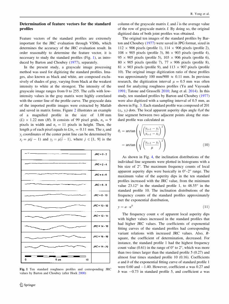
Determination of feature vectors for the standardprofiles

Feature vectors of the standard profiles are extremely

important for the JRC evaluation through VSMs, which

determines the accuracy of the JRC evaluation result. In

order reasonably to determine the feature vector, it is

necessary to study the standard profiles (Fig. 1), as intro-

duced by Barton and Choubey (1977), separately.

In the present study, a grayscale image processing

method was used for digitizing the standard profiles. Ima-

ges, also known as black and white, are composed exclu-

sively of shades of gray, varying from black at the weakest

intensity to white at the strongest. The intensity of the

grayscale image ranges from 0 to 255. The cells with low-

intensity values in the gray matrix were highly correlated

with the center line of the profile curve. The grayscale data

of the imported profile images were extracted by Matlab

and saved in matrix forms. Figure 2 illustrates an example

of a magnified profile in the size of 1.00 mm

(L) 9 1.22 mm (H). It consists of 99 pixel grids, nx = 9

pixels in width and ny = 11 pixels in height. Then, the

length l of each pixel equals to L/nx = 0.11 mm. The xj and

yj coordinates of the center point line can be determined by

xj = l(j - 1) and yj ¼ lð�i� 1Þ, where j 2 [1, 9] is the

column of the grayscale matrix I, and �i is the average value

of the row of grayscale matrix I. By doing so, the original

digitized data of both joint profiles was obtained.

The original ten images of the standard profiles by Bar-

ton and Choubey (1977) were saved in JPG format, sized in

112 9 906 pixels (profile 1), 114 9 906 pixels (profile 2),




81 9 903 pixels (profile 9), and 113 9 907 pixels (profile

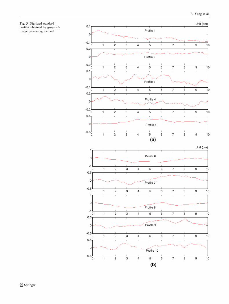
10). The original image digitization ratio of these profiles

was approximately 100 mm/900 & 0.11 mm. In previous

research, the digitization interval l = 0.5 mm was often

used for analyzing roughness profiles (Yu and Vayssade

1991; Tatone and Grasselli 2010; Jang et al. 2014). In this

study, ten standard profiles by Barton and Choubey (1977)

were also digitized with a sampling interval of 0.5 mm, as

shown in Fig. 3. Each standard profile was composed of 201

(xi, yi) dots. The local apparent asperity dips angle hiof theline segment between two adjacent points along the stan-

dard profile was calculated as

hi ¼ arctan

ffiffiffiffiffiffiffiffiffiffiffiffiffiffiffiffiffiffiffiffiffiffiffiffiffiffi

yiþ1 � yi

xiþ1 � xi

� �2s

0

@

1

A

¼ arctan

ffiffiffiffiffiffiffiffiffiffiffiffiffiffiffiffiffiffiffiffiffiffiffiffiffiffi

yiþ1 � yi

l

� �2s

0

@

1

A ð10Þ

As shown in Fig. 4, the inclination distributions of the

individual line segments were plotted in histograms with a

bin size of 2�. The maximum frequency counts of local

apparent asperity dips were basically in 0�–2� range. The

maximum value of the asperity dips in the ten standard

profiles increased with the JRC value, from the minimum

value 23.12� in the standard profile 1, to 48.55� in the

standard profile 10. The inclination distributions of the

frequency counts of the standard profiles approximately

met the exponential distribution,

y ¼ a � jb ð11Þ

The frequency count j of apparent local asperity dips

with higher values increased in the standard profiles that

had higher JRC values. The coefficients of exponential

fitting curves of the standard profiles had corresponding

variant relations with increased JRC values. Also, R-

square, the coefficient of determination, decreased. For

instance, the standard profile 1 had the highest frequency

count value (0.61) in the range of 0� to 2�, which was more

than two times larger than the standard profile 5 (0.27) and

almost four times standard profile 10 (0.16). Coefficients

a and b of the exponential fitting curve of standard profile 1

were 0.60 and -1.40. However, coefficient a was 0.27 and

b was -0.73 in standard profile 5, and coefficient a wasFig. 1 Ten standard roughness profiles and corresponding JRC

values by Barton and Choubey (after Hoek 2000)

R. Yong et al.

123

0.15 and b was -0.49 in standard profile 10. R-square

decreased from 0.94 in standard profile 1 and to 0.66 in

standard profile 10. The frequency counts of local apparent

asperity dips in standard profile 10 varied from 0� to 50�,but the counts of the standard profile 1 were mainly in the

range of 0�–24�. The results indicated that the ten standard

profiles had distinctly different inclination distributions.

Moreover, they illustrated the geometric irregularities

(waves) differences between Barton’s standard profiles.

The inclination distributions are presented as the feature

vectors S* with the interval of 2�. For convenient evalua-tion of the similarity measures, the inclination distributions

were normalized by the following equation:

si ¼s�i � S�min

S�max � S�min

; ð12Þ

where the element si is the result after normalizing vector

S*, si* is the count value of local apparent asperity dips in

every 2 degrees, Smin* and Smax

* are the minimum value and

the maximum value of local apparent asperity dips in the

vector S*, respectively. It is important to clarify that

additional local apparent asperity dips ranging between 0�and 2� may appear due to the low image accuracy of the

standard profiles; these asperity dips have not been con-

sidered in the feature vector of the inclination distribution.

The normalized feature vector S is tabulated in Table 1.

Similarity measures for JRC evaluation

Determination of feature vector for test profiles

The test sample profiles were obtained from natural

rock joints with different surface characteristics using

the mechanical hand profilograph (Du et al. 2009;

Morelli 2014). The rough and irregular profiles were

obtained from the bedding joints of Granite. The rough

and undulating profiles were obtained from the tectonic

joints of Limestone. The smooth, planar profiles were

obtained from the cleavage joints of slate. These

sample profiles were 10 cm long, identical to the

standard profiles of Barton and Choubey (1977). The

sample profiles were digitized using a similar grayscale

image processing method as described in Sect. 3 for

the standard profiles.

Furthermore, the inclination distributions were pre-

sented as a 15-dimensional feature vector T with the

interval of 2�. For a convenient evaluation of the similarity

measures, the feature vectors of the inclination distribu-

tions were expressed by the following equation:

ti ¼t�i � S�min

S�max � S�min

: ð13Þ

For the test profiles, ti* represents the count value of

asperity dips in every 2�. The feature vectors of the test

profiles are listed in Table 2. The similarity values were

obtained by similarity measures between the feature vec-

tors Sk (1, 2,…, 10) of the standard profiles and test profiles

Tj (j = 1, 2,…, 9).

JRC evaluation result

The similarity measure values of vk = J(Sk, Tj), D(Sk, Tj),

C(Sk, Tj) (k = 1, 2, …, 10; j = 1, 2, …, 9) were obtained

by Eqs. (7), (8), (9) and the range of the vk was normalized

from [0, 1] into [–1, 1] for convenient evaluation by the

following relation index:

Fig. 2 Schematic diagram of

principle of the joint roughness

profile digitization method on

the basis of image pixel

analysis. a Grayscale image of

the joint profile; b magnified

zoom in 1 cm length; c gray

matrix; d the digitized points


123

0 1 2 3 4 5 6 7 8 9 10-0.1

0

0.1

0 1 2 3 4 5 6 7 8 9 10-0.2

0

0.2

0 1 2 3 4 5 6 7 8 9 10-0.1

0

0.1

0 1 2 3 4 5 6 7 8 9 10-0.2

0

0.2

0 1 2 3 4 5 6 7 8 9 10-0.5

0

0.5

(a)

Unit (cm)

Profile 1

Profile 2

Profile 3

Profile 4

Profile 5

0 1 2 3 4 5 6 7 8 9 10-1

0

1

0 1 2 3 4 5 6 7 8 9 10-0.5

0

0.5

0 1 2 3 4 5 6 7 8 9 10-1

0

1

0 1 2 3 4 5 6 7 8 9 10-0.5

0

0.5

0 1 2 3 4 5 6 7 8 9 10-0.5

0

0.5

(b)

Unit (cm)

Profile 6

Profile 7

Profile 8

Profile 9

Profile 10

Fig. 3 Digitized standard

profiles obtained by grayscale

image processing method

R. Yong et al.

123

0 5 10 15 20 25 30 35 40 45 500.00

0.05

0.10

0.15

0.20

0.6Standard Profile 1

Rel

ativ

e Fr

eque

ncy

Local Apparent Asperity Dip (°)

1.398

2

0.599

0.936

y x

R

(a)

0 5 10 15 20 25 30 35 40 45 500.00

0.05

0.10

0.15

0.20

0.35

0.40

0.45

(b)

Standard Profile 2

0.998

2

0.428

0.910

y x

R

Rel

ativ

e Fr

eque

ncy


0 5 10 15 20 25 30 35 40 45 500.00

0.05

0.10

0.15

0.20

0.35

0.40

0.45

(c)

Standard Profile 3

0.983

2

0.403

0.875

y x

R

Rel

ativ

e Fr

eque

ncy

Local Apparent Asperity Dip (°)0 5 10 15 20 25 30 35 40 45 50

0.00

0.05

0.10

0.15

0.20

0.25

0.30

(d)

Standard Profile 4

0.693

2

0.250

0.766

y x

R

Rel

ativ

e Fr

eque

ncy


0 5 10 15 20 25 30 35 40 45 500.00

0.05

0.10

0.15

0.20

0.25

0.30

(e)

Standard Profile 5

0.729

2

0.267

0.730

y x

R

Rel

ativ

e Fr

eque

ncy


0.00

0.05

0.10

0.15

0.20

0.25

0.30

(f)

Standard Profile 6

0.722

2

0.254

0.772

y x

R

Rel

ativ

e Fr

eque

ncy


Fig. 4 Inclination distributions of the individual line segments of each standard profile


123

rk ¼2vk � vmin � vmax

vmax � vmin

: ð14Þ

where the vmax and vmin are the maximum and minimum

values of the similarity measure value vk.

If the relation index rk has the negative value of -1, the

test profile for Tj does not have identical roughness with the

k-th standard JRC profile. But, if the relation index rk has

the positive value of 1, the test profile for Tj has identical

roughness with the k-th standard JRC profile. By using

Eq. (14), the relation indices are shown in Table 3. The

JRC values can be confirmed according to the maximum

relation index. The JRC evaluation process by VSMs and

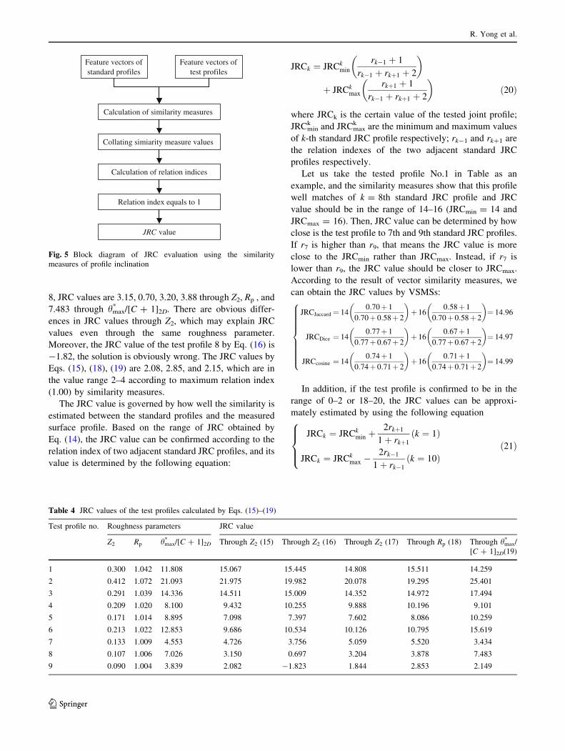
relation indices is shown in Fig. 5.

For rough and irregular profiles, the JRC values of test

profiles 1 and 3 are 14–16 according to the maximum

relation index (1.00). This indicates that these two profiles

have identical roughness with the 8th standard profile from

the irregularity characteristics. The JRC value of test pro-

file 2 is 18–20 according to the maximum relation index

(1.00). This indicates that this profile has identical rough-

ness with the 10th standard profile. The irregularity char-

acteristics of this test profile are quite different from

standard profile 1–3, and negative relation indices are

obtained by VSMs method.

For rough and undulating profiles, Table 3 shows that

the JRC values of profiles 4 and 6 are 10–12. This indicates

that they have identical roughness with standard profile 6.

The test profile 5 has a JRC value in the range of 6–8. This

indicates that it has an identical roughness with standard

profile 4. The JRC values of 0–2, 2–4, 12–14, 16–18,

0 5 10 15 20 25 30 35 40 45 500.00

0.05

0.10

0.15

0.20

0.25

0.30

(g)

Standard Profile 7

0.562

2

0.179

0.657

y x

R

Rel

ativ

e Fr

eque

ncy


0.00

0.05

0.10

0.15

0.20

0.25

0.30

(h)

Standard Profile 8

0.512

2

0.163

0.681

y x

R

Rel

ativ

e Fr

eque

ncy


0 5 10 15 20 25 30 35 40 45 500.00

0.05

0.10

0.15

0.20

0.25

0.30

(i)

Standard Profile 9

0.484

2

0.152

0.509

y x

R

Rel

ativ

e Fr

eque

ncy


0.00

0.05

0.10

0.15

0.20

0.25

0.30

(j)

Standard Profile 10

0.491

2

0.150

0.657

y x

R

Rel

ativ

e Fr

eque

ncy


Fig. 4 continued

R. Yong et al.

123

18–20 show very low possibility due to the negative

relation indices.

For smooth and even profiles, there is little difference in

JRC values of test profile 7 among the results using the

Jaccard similarity measure, Dice similarity measure, and

cosine similarity. According to the results obtained through

the cosine measure, the JRC value of this profile roughness

is 4–6 according to maximum relation index (1.00), the

second maximum relation is 0.95 (JRC 6–8). The maxi-

mum relation index (1.00) obtained through the Jaccard

similarity measure and Dice similarity measure have

identical roughness with the JRC 6–8, and the second

maximum relation is 0.93 and 0.94 (JRC 4–6), respec-

tively. The difference between the maximum and the

second maximum relation index was observed to be min-

imal and insignificant for the overall results. This agrees

with Ye (2014) who has pointed out that the Jaccard and

Dice similarity measures are better than the cosine method

in the similarity identification. The JRC values of test

profiles 8 and 9 are 2–4 due to maximum relation index

(1.00). This indicates that these profiles have identical

roughness as the 2nd standard profile, and the JRC values

of 8–10, 10–12, 12–14, 14–16, 16–18, and 18–20 have

very low possibility due to the negative relation indices.

Comparisons with other measures for JRC

It has long been recognized that sampling interval plays an

important role in obtaining accurate estimations for

roughness parameters (Yu and Vayssade 1991; Yang et al.

2001a, b; Tatone and Grasselli 2010; Jang et al. 2014;

Fathi et al. 2016). However, to date, there are no widely

adopted methods or suggested guidelines to determine the

reasonable resolution for the measurement of discontinuity

roughness (Tatone and Grasselli 2013). To solve this

problem, the empirical equations for estimating JRC are

generally studied by a certain sampling interval. In engi-

neering practice, the joint profiles are usually measured by

the profile comb which is only capable of obtaining mea-

surements at a certain horizontal interval between 0.5 and

1 mm. The sampling interval of 0.5 mm could indicate

more detailed geometric irregularities of joint surfaces and

the correlations between statistical parameters and JRC

values were studied using the same sampling interval in

previous literature (e.g. Yu and Vayssade 1991; Yang et al.

2001a, b; Tatone and Grasselli 2010). Therefore, a sam-

pling interval of 0.5 mm was used in this study and the

JRC values can be calculated by following equations:

JRC ¼ 61:79 � Z2 � 3:47; ð15ÞJRC ¼ 32:69þ 32:98 � log10 Z2; ð16Þ

JRC ¼ 51:85ðZ2Þ0:60 � 10:37: ð17Þ

Table

1Norm

alized

feature

vectors

oftheinclinationdistributionfortenstandardprofiles

No.

JRC

value

Feature

vectorSk

Standardprofile

10–2

[0.00,0.29,0.60,0.89,0.09,0.11,0.20,0.06,0.00,0.00,0.00,0.03,0.00,0.00,0.00,0.00,0.00,0.00,0.00,0.00,0.00,0.00,0.00,0.00,0.00]

Standardprofile

22–4

[0.00,0.69,0.49,1.00,0.17,0.23,0.34,0.11,0.11,0.03,0.00,0.03,0.03,0.06,0.00,0.00,0.00,0.00,0.00,0.00,0.00,0.00,0.00,0.00,0.00]

Standardprofile

34–6

[0.00,0.34,0.63,0.89,0.26,0.37,0.49,0.11,0.06,0.14,0.06,0.03,0.00,0.00,0.00,0.00,0.00,0.00,0.00,0.00,0.00,0.00,0.00,0.00,0.00]

Standardprofile

46–8

[0.00,0.37,0.66,0.89,0.49,0.40,0.43,0.17,0.20,0.14,0.23,0.06,0.09,0.09,0.06,0.03,0.00,0.00,0.03,0.00,0.00,0.00,0.00,0.00,0.00]

Standardprofile

58–10

[0.00,0.26,0.60,0.91,0.49,0.43,0.57,0.29,0.20,0.17,0.06,0.14,0.03,0.00,0.00,0.00,0.00,0.00,0.00,0.00,0.00,0.03,0.00,0.00,0.00]

Standardprofile

610–12

[0.00,0.29,0.69,0.46,0.43,0.17,0.69,0.17,0.17,0.34,0.26,0.17,0.14,0.17,0.03,0.00,0.06,0.00,0.00,0.00,0.00,0.00,0.00,0.00,0.00]

Standardprofile

712–14

[0.00,0.23,0.46,0.57,0.26,0.29,0.60,0.40,0.20,0.31,0.29,0.23,0.29,0.20,0.09,0.14,0.03,0.00,0.03,0.06,0.00,0.00,0.00,0.00,0.00]

Standardprofile

814–16

[0.00,0.43,0.46,0.57,0.43,0.49,0.57,0.23,0.31,0.14,0.20,0.20,0.23,0.14,0.17,0.11,0.09,0.03,0.03,0.00,0.00,0.03,0.00,0.00,0.00]

Standardprofile

916–18

[0.00,0.26,0.49,0.77,0.23,0.34,0.37,0.23,0.51,0.29,0.40,0.17,0.40,0.17,0.00,0.11,0.00,0.06,0.03,0.00,0.03,0.00,0.00,0.00,0.03]

Standardprofile

10

18–20

[0.00,0.34,0.26,0.49,0.23,0.26,0.49,0.26,0.29,0.46,0.34,0.26,0.14,0.11,0.20,0.06,0.17,0.17,0.09,0.03,0.03,0.11,0.03,0.00,0.03]


123

When sampling interval is 0.5 mm, the equation for

estimating JRC from Rp is

JRC ¼ 3:36� 10�2 þ 1:27� 10�3

lnðRpÞ

� ��1

: ð18Þ

The equation by Tatone and Grasselli (2010) to estimate

JRC for sampling interval of 0.5 mm is expressed as

JRC ¼ 3:95ðh�max=½C þ 1�2DÞ0:7 � 7:98: ð19Þ

Table 4 presents the roughness parameters Z2, Rp, hmax* /

[C ? 1]2D, and the results of JRC validation through the

Eqs. (15)–(19). For test profile 1, the minimum JRC values

and maximum value by roughness parameters are 14.26

and 15.51, respectively, which is within the JRC 14–16

range by similarity measures. For test profile 2, the JRC

values obtained by Eqs. (15)–(19) are 21.96, 19.98, 20.08,

19.30, 25.40, respectively. However, according to the JRC

evaluation method by Barton and Choubey (1977), the

Table 2 Normalized feature vectors of the inclination distribution of the test profiles

Test Profile NO.

rotceverutaeF)mc(eliforpssenhguordezitigiDnoitpircseD Tj

1 Granite: rough, irregular,

bedding joints

0 2 4 6 8 10-0.5

0

0.5

1

[0.00,0.23,0.29,0.31,0.49,0.54,0.29,0.26,0.34,0.29,0.34,0.26,0.09,0.11,0.11,0.09,0.03,0.09,0.06,0.00,0.00,0.00,0.03,0.00,0.00]


bedding joints

0 2 4 6 8 10-1

-0.5

0

0.5

[0.00,0.09,0.17,0.20,0.60,0.17,0.06,0.20,0.60,1.43,0.17,0.11,0.23,0.17,0.11,0.09,0.06,0.03,0.00,0.03,0.03,0.03,0.06,0.00,0.03]


bedding joints

0 2 4 6 8 100

0.5

1

1.5

[0.00,0.40,0.49,0.20,0.54,0.94,0.06,0.31,0.17,0.34,0.09,0.23,0.09,0.11,0.06,0.11,0.03,0.09,0.06,0.00,0.00,0.03,0.00,0.03,0.03]

4 Limestone: rough,

undulating, tectonic joints

0 2 4 6 8 10-0.5

0

0.5

1

[0.00,0.26,1.00,0.09,0.60,0.54,0.17,0.17,0.09,0.11,0.06,0.03,0.03,0.06,0.06,0.03,0.03,0.00,0.03,0.00,0.00,0.00,0.00,0.00,0.06]

5 Limestone: rough, planar,

tectonic joints

0 2 4 6 8 100

0.2

0.4

[0.00,0.34,0.74,0.26,1.37,0.14,0.20,0.03,0.29,0.14,0.09,0.03,0.09,0.00,0.03,0.00,0.03,0.00,0.00,0.00,0.00,0.00,0.00,0.00,0.00]

6 Limestone: rough,

undulating, tectonic joints

0 2 4 6 8 10-0.2

0

0.2

0.4

[0.00,0.26,1.00,0.09,0.60,0.54,0.17,0.17,0.09,0.11,0.06,0.03,0.03,0.06,0.06,0.03,0.03,0.00,0.03,0.00,0.00,0.00,0.00,0.00,0.06]

7 Slate: smooth, planar:

cleavage joints

0 2 4 6 8 10-0.2

0

0.2

[0.00,0.31,1.51,0.37,0.20,0.63,0.20,0.11,0.11,0.03,0.06,0.03,0.03,0.00,0.00,0.00,0.00,0.00,0.00,0.00,0.00,0.00,0.00,0.00,0.00]


cleavage joints

0 2 4 6 8 10-0.2

0

0.2

[0.00,1.91,1.03,0.54,0.34,0.11,0.26,0.09,0.00,0.03,0.03,0.00,0.00,0.00,0.00,0.00,0.00,0.00,0.00,0.00,0.00,0.00,0.00,0.00,0.00]


cleavage joints

0 2 4 6 8 10

-0.2

0

0.2

[0.00,1.57,0.83,0.97,0.40,0.06,0.09,0.03,0.00,0.00,0.00,0.00,0.00,0.00,0.00,0.00,0.00,0.00,0.00,0.00,0.00,0.00,0.00,0.00,0.00]

R. Yong et al.

123

maximum JRC value should be in the range of 18–20.

Thus, the suggested JRC value by similarity measures in

this paper is 18–20. For the test profile 3, the JRC values

based on roughness parameters are 14.51, 15.01, 14.35,

14.97, and 17.49. The JRC value of this profile roughness

suggested by this paper is 14–16 due to maximum relation

index (1.00). The results by Eqs. (15), (16), (17), and (18)

are in the suggested range and JRC through hmax* /[C ? 1]2D

is little higher. Because feature vectors refer to the absolute

angle of the line segment between two adjacent points

along the standard profile, the same part in roughness

parameters Z2, Rp. But the angle value is considered to be

positive or negative in roughness parameter hmax* /

[C ? 1]2D according to the shear directions. For test profile

4, the JRC values by roughness parameters are 9.43, 10.26,

9.88, 10.20, 9.10, which are in the value range 10–12 due

to maximum relation index (1.00) by similarity measures.

For test profile 5, the JRC value by similarity measures has

identical roughness with the 4th standard JRC profile (6–8).

The JRC values through Z2, Rp are 7.10, 7.40, 7.60, and

8.09. The JRC values of test profile 6 are 9.68, 10.53,

10.13, 10.795, 15.62 through roughness parameters. How-

ever, the suggested JRC value of test profile 6 is between

10 and 12, which is the same as test profile 4. For test

profile 7, the JRC values by roughness parameters are

4.726, 3.76, 5.06, 5.52, and 3.43, respectively. As we

know, the JRC value suggested by the cosine measure is

4-6, due to maximum relation index (1.00). Therefore, the

JRC values by Eqs. (15), (17) and (18) were also within

this range. However, the results using the Jaccard and Dice

similarity measure range between JRC 6 and JRC 8, which

are higher than the values obtained by roughness parame-

ters. Nevertheless, different methods of measurement may

indicate the difference in the evaluation results. The Jac-

card and Dice similarity measures imply stronger identifi-

cation than the cosine measure (Ye 2014). For test profile

Table 3 Results of JRC evaluation by vector similarity measures

Test

(profile) no.

Method Relation indices (rk) JRC diagnosis

resultJRC

(0–2)

JRC

(2–4)

JRC

(4–6)

JRC

(6–8)

JRC

(8–10)

JRC

(10–12)

JRC

(12–14)

JRC

(14–16)

JRC

(16–18)

JRC

(18–20)

1 rJaccard -1.00 -0.64 -0.15 0.40 0.27 0.41 0.70 1.00 0.58 0.87 JRC (14–16)

rDice -1.00 -0.55 -0.01 0.51 0.40 0.53 0.77 1.00 0.67 0.90 JRC (14–16)

rcosine -1.00 -0.51 0.00 0.57 0.48 0.52 0.74 1.00 0.71 0.85 JRC (14–16)

2 rJaccard -1.00 -0.73 -0.42 0.02 0.00 0.49 0.50 0.24 0.66 1.00 JRC (18–20)

rDice -1.00 -0.66 -0.29 0.16 0.14 0.59 0.60 0.37 0.73 1.00 JRC (18–20)

rcosine -1.00 -0.72 -0.35 0.06 0.03 0.52 0.55 0.29 0.62 1.00 JRC (18–20)

3 rJaccard -1.00 -0.50 0.02 0.52 0.41 0.12 0.28 1.00 0.18 0.23 JRC (14–16)

rDice -1.00 -0.40 0.14 0.61 0.50 0.24 0.39 1.00 0.30 0.35 JRC (14–16)

rcosine -1.00 -0.45 0.12 0.59 0.49 0.22 0.38 1.00 0.27 0.37 JRC (14–16)

4 rJaccard -0.83 -0.94 0.33 0.93 0.54 1.00 -0.17 0.71 -0.56 -1.00 JRC (10–12)

rDice -0.80 -0.93 0.40 0.94 0.59 1.00 -0.10 0.75 -0.50 -1.00 JRC (10–12)

rcosine -0.75 -0.96 0.39 0.96 0.61 1.00 -0.11 0.74 -0.52 -1.00 JRC (10–12)

5 rJaccard -1.00 -0.62 -0.07 1.00 0.69 0.89 -0.35 0.61 -0.31 -0.67 JRC (6–8)

rDice -1.00 -0.56 0.02 1.00 0.74 0.91 -0.26 0.66 -0.22 -0.62 JRC (6–8)

rcosine -1.00 -0.73 -0.03 1.00 0.69 0.99 -0.32 0.69 -0.37 -0.65 JRC (6–8)

6 rJaccard -1.00 -0.76 0.07 0.92 0.67 1.00 -0.25 0.52 -0.55 -0.82 JRC (10–12)

rDice -1.00 -0.72 0.16 0.94 0.71 1.00 -0.16 0.59 -0.49 -0.78 JRC (10–12)

rcosine -0.97 -1.00 0.05 0.79 0.52 1.00 -0.27 0.50 -0.76 -0.85 JRC (10–12)

7 rJaccard 0.34 0.08 0.93 1.00 0.69 0.59 -0.17 0.29 -0.06 -1.00 JRC (6–8)

rDice 0.42 0.17 0.94 1.00 0.74 0.65 -0.08 0.38 0.04 -1.00 JRC (6–8)

rcosine 0.73 0.11 1.00 0.95 0.66 0.69 -0.07 0.36 -0.05 -1.00 JRC (4–6)

8 rJaccard -0.36 1.00 0.01 0.14 -0.33 -0.36 -0.93 -0.19 -0.85 -1.00 JRC (2–4)

rDice -0.28 1.00 0.10 0.24 -0.24 -0.27 -0.92 -0.09 -0.83 -1.00 JRC (2–4)

rcosine 0.11 1.00 0.13 0.09 -0.45 -0.28 -0.95 -0.13 -1.00 -0.91 JRC (2–4)

9 rJaccard -0.03 1.00 0.09 0.18 -0.20 -0.60 -0.93 -0.37 -0.70 -1.00 JRC (2–4)

rDice 0.10 1.00 0.22 0.30 -0.08 -0.51 -0.91 -0.25 -0.63 -1.00 JRC (2–4)

rcosine 0.43 1.00 0.22 0.17 -0.26 -0.59 -1.00 -0.33 -0.80 -1.00 JRC (2–4)


123

8, JRC values are 3.15, 0.70, 3.20, 3.88 through Z2, Rp , and

7.483 through hmax* /[C ? 1]2D. There are obvious differ-

ences in JRC values through Z2, which may explain JRC

values even through the same roughness parameter.

Moreover, the JRC value of the test profile 8 by Eq. (16) is

-1.82, the solution is obviously wrong. The JRC values by

Eqs. (15), (18), (19) are 2.08, 2.85, and 2.15, which are in

the value range 2–4 according to maximum relation index

(1.00) by similarity measures.

The JRC value is governed by how well the similarity is

estimated between the standard profiles and the measured

surface profile. Based on the range of JRC obtained by

Eq. (14), the JRC value can be confirmed according to the

relation index of two adjacent standard JRC profiles, and its

value is determined by the following equation:

JRCk ¼ JRCkmin

rk�1 þ 1

rk�1 þ rkþ1 þ 2

� �

þ JRCkmax

rkþ1 þ 1

rk�1 þ rkþ1 þ 2

� �

ð20Þ

where JRCk is the certain value of the tested joint profile;

JRCmink and JRCmax

k are the minimum and maximum values

of k-th standard JRC profile respectively; rk-1 and rk?1 are

the relation indexes of the two adjacent standard JRC

profiles respectively.

Let us take the tested profile No.1 in Table as an

example, and the similarity measures show that this profile

well matches of k = 8th standard JRC profile and JRC

value should be in the range of 14–16 (JRCmin = 14 and

JRCmax = 16). Then, JRC value can be determined by how

close is the test profile to 7th and 9th standard JRC profiles.

If r7 is higher than r9, that means the JRC value is more

close to the JRCmin rather than JRCmax. Instead, if r7 is

lower than r9, the JRC value should be closer to JRCmax.

According to the result of vector similarity measures, we

can obtain the JRC values by VSMSs:

JRCJaccard ¼ 140:70þ 1

0:70þ 0:58þ 2

� �

þ 160:58þ 1

0:70þ 0:58þ 2

� �

¼ 14:96

JRCDice ¼ 140:77þ 1

0:77þ 0:67þ 2

� �

þ 160:67þ 1

0:77þ 0:67þ 2

� �

¼ 14:97

JRCcosine ¼ 140:74þ 1

0:74þ 0:71þ 2

� �

þ 160:71þ 1

0:74þ 0:71þ 2

� �

¼ 14:99

8

>

>

>

>

>

>

>

>

<

>

>

>

>

>

>

>

>

:

In addition, if the test profile is confirmed to be in the

range of 0–2 or 18–20, the JRC values can be approxi-

mately estimated by using the following equation

JRCk ¼ JRCkmin þ

2rkþ1

1þ rkþ1

ðk ¼ 1Þ

JRCk ¼ JRCkmax �

2rk�1

1þ rk�1

ðk ¼ 10Þ

8

>

>

<

>

>

:

ð21Þ

Feature vectors of standard profiles

Feature vectors of test profiles

Calculation of similarity measures

Collating simiarity measure values

Relation index equals to 1

JRC value

Calculation of relation indices

Fig. 5 Block diagram of JRC evaluation using the similarity

measures of profile inclination

Table 4 JRC values of the test profiles calculated by Eqs. (15)–(19)

Test profile no. Roughness parameters JRC value

Z2 Rp hmax* /[C ? 1]2D Through Z2 (15) Through Z2 (16) Through Z2 (17) Through Rp (18) Through hmax

* /

[C ? 1]2D(19)

1 0.300 1.042 11.808 15.067 15.445 14.808 15.511 14.259

2 0.412 1.072 21.093 21.975 19.982 20.078 19.295 25.401

3 0.291 1.039 14.336 14.511 15.009 14.352 14.972 17.494

4 0.209 1.020 8.100 9.432 10.255 9.888 10.196 9.101

5 0.171 1.014 8.895 7.098 7.397 7.602 8.086 10.259

6 0.213 1.022 12.853 9.686 10.534 10.126 10.795 15.619

7 0.133 1.009 4.553 4.726 3.756 5.059 5.520 3.434

8 0.107 1.006 7.026 3.150 0.697 3.204 3.878 7.483

9 0.090 1.004 3.839 2.082 -1.823 1.844 2.853 2.149

R. Yong et al.

123

The distribution of the JRC values calculated via the

statistical methods and VSMs are shown in Fig. 6. The

predictions of JRC values from Eq. (20) agree well with

the calculated values based on the relations with roughness

parameters.

Discussion

The roughness profile of a natural rock joint surface is

continuous, the digitized roughness profile data obtained

through measurement devices are available only at a cer-

tain interval of horizontal spacing. Figure 7 shows an

example of generating profiles in different resolutions, and

three processed profiles generated via the random midpoint

displacement method (Kulatilake and Um 1999). The

profile becomes smoother under larger sampling interval,

and the subprime irregular undulations between smaller

horizontal spacing were neglected. Hence, the JRC values

of test profiles depend on the chosen sampling interval,

which means the calculated JRC values vary according to

the used sampling interval.

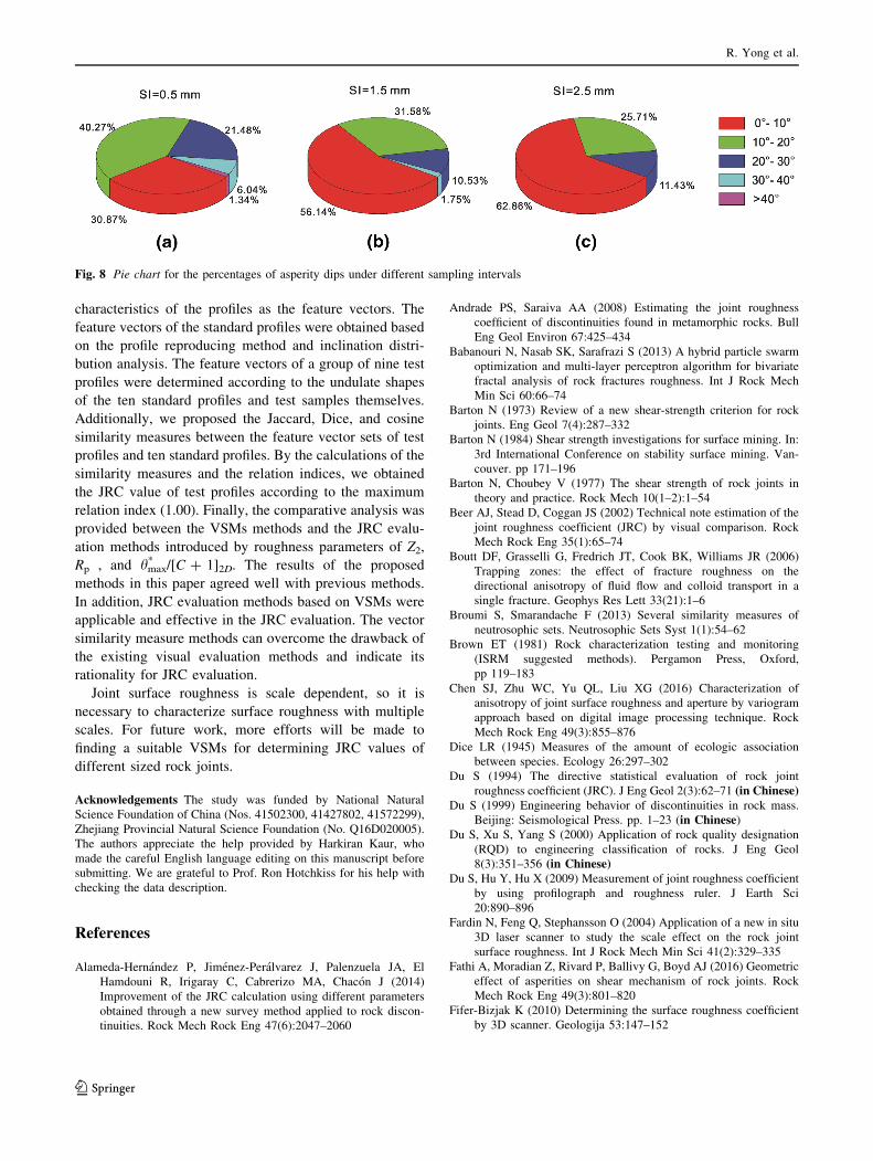
Three different sampling intervals including 0.5, 1.5,

and 2.5 mm are used to indicate the angular variation of

line segments along the test joint profile No.1. The

asperity dips were calculated by Eq. (10), and the fre-

quency counts were grouped by angularly spaced dips. As

shown in Fig. 8, the percentage of the asperity dips in

range of 0�–10� increase with the sampling interval, but

the percentage of high asperity dips reduces. By 0.5 mm

sampling interval, there are 1.34% asperity dips large than

40� and 6.04% in range of 30�–40�. The percentage of

asperity dips in range of 30�–40� decreases to 1.75% and

no asperity dip exceeds 40� when using the sampling

interval of 1.5 mm. All of asperity dips are smaller than

30� by 2.5 mm sampling interval. According to the sim-

ilarity theory, the feature vectors should represent the

characters of object exactly. The feature values corre-

spond to the distributions of the asperity dips here. The

distributions under 0.5 mm sampling interval show much

more detailed geometric irregularities (waves) of rock

joints. However, the larger sampling interval makes the

feature vector less accurate.

Conclusions

JRC is one of the most important parameters utilized in

calculating shear strength of rough joints in rock masses. In

this study, VSMs are suggested for estimating the JRC

value on the basis of the standard profiles introduced by

Barton and Choubey (1977). The angular variation of line

segments was used to represent the irregularity

Fig. 6 JRC values of the test

profiles calculated by Eqs. (15)–

(19) and VSMs methods

Fig. 7 Generation of the digitized profiles by various sampling

intervals (after Kulatilake and Um 1999)


123

characteristics of the profiles as the feature vectors. The

feature vectors of the standard profiles were obtained based

on the profile reproducing method and inclination distri-

bution analysis. The feature vectors of a group of nine test

profiles were determined according to the undulate shapes

of the ten standard profiles and test samples themselves.

Additionally, we proposed the Jaccard, Dice, and cosine

similarity measures between the feature vector sets of test

profiles and ten standard profiles. By the calculations of the

similarity measures and the relation indices, we obtained

the JRC value of test profiles according to the maximum

relation index (1.00). Finally, the comparative analysis was

provided between the VSMs methods and the JRC evalu-

ation methods introduced by roughness parameters of Z2,

Rp , and hmax* /[C ? 1]2D. The results of the proposed

methods in this paper agreed well with previous methods.

In addition, JRC evaluation methods based on VSMs were

applicable and effective in the JRC evaluation. The vector

similarity measure methods can overcome the drawback of

the existing visual evaluation methods and indicate its

rationality for JRC evaluation.

Joint surface roughness is scale dependent, so it is

necessary to characterize surface roughness with multiple

scales. For future work, more efforts will be made to

finding a suitable VSMs for determining JRC values of

different sized rock joints.

Acknowledgements The study was funded by National Natural

Science Foundation of China (Nos. 41502300, 41427802, 41572299),

Zhejiang Provincial Natural Science Foundation (No. Q16D020005).

The authors appreciate the help provided by Harkiran Kaur, who

made the careful English language editing on this manuscript before

submitting. We are grateful to Prof. Ron Hotchkiss for his help with

checking the data description.

References

Alameda-Hernandez P, Jimenez-Peralvarez J, Palenzuela JA, El

Hamdouni R, Irigaray C, Cabrerizo MA, Chacon J (2014)

Improvement of the JRC calculation using different parameters

obtained through a new survey method applied to rock discon-

tinuities. Rock Mech Rock Eng 47(6):2047–2060

Andrade PS, Saraiva AA (2008) Estimating the joint roughness

coefficient of discontinuities found in metamorphic rocks. Bull

Eng Geol Environ 67:425–434

Babanouri N, Nasab SK, Sarafrazi S (2013) A hybrid particle swarm

optimization and multi-layer perceptron algorithm for bivariate

fractal analysis of rock fractures roughness. Int J Rock Mech

Min Sci 60:66–74

Barton N (1973) Review of a new shear-strength criterion for rock

joints. Eng Geol 7(4):287–332

Barton N (1984) Shear strength investigations for surface mining. In:

3rd International Conference on stability surface mining. Van-

couver. pp 171–196

Barton N, Choubey V (1977) The shear strength of rock joints in

theory and practice. Rock Mech 10(1–2):1–54

Beer AJ, Stead D, Coggan JS (2002) Technical note estimation of the

joint roughness coefficient (JRC) by visual comparison. Rock

Mech Rock Eng 35(1):65–74

Boutt DF, Grasselli G, Fredrich JT, Cook BK, Williams JR (2006)

Trapping zones: the effect of fracture roughness on the

directional anisotropy of fluid flow and colloid transport in a

single fracture. Geophys Res Lett 33(21):1–6

Broumi S, Smarandache F (2013) Several similarity measures of

neutrosophic sets. Neutrosophic Sets Syst 1(1):54–62

Brown ET (1981) Rock characterization testing and monitoring

(ISRM suggested methods). Pergamon Press, Oxford,

pp 119–183

Chen SJ, Zhu WC, Yu QL, Liu XG (2016) Characterization of

anisotropy of joint surface roughness and aperture by variogram

approach based on digital image processing technique. Rock


Dice LR (1945) Measures of the amount of ecologic association

between species. Ecology 26:297–302

Du S (1994) The directive statistical evaluation of rock joint

roughness coefficient (JRC). J Eng Geol 2(3):62–71 (in Chinese)Du S (1999) Engineering behavior of discontinuities in rock mass.

Beijing: Seismological Press. pp. 1–23 (in Chinese)Du S, Xu S, Yang S (2000) Application of rock quality designation

(RQD) to engineering classification of rocks. J Eng Geol

8(3):351–356 (in Chinese)Du S, Hu Y, Hu X (2009) Measurement of joint roughness coefficient

by using profilograph and roughness ruler. J Earth Sci

20:890–896

Fardin N, Feng Q, Stephansson O (2004) Application of a new in situ

3D laser scanner to study the scale effect on the rock joint

surface roughness. Int J Rock Mech Min Sci 41(2):329–335

Fathi A, Moradian Z, Rivard P, Ballivy G, Boyd AJ (2016) Geometric

effect of asperities on shear mechanism of rock joints. Rock


Fifer-Bizjak K (2010) Determining the surface roughness coefficient

by 3D scanner. Geologija 53:147–152

Fig. 8 Pie chart for the percentages of asperity dips under different sampling intervals

R. Yong et al.

123

Gao Y, Ngai L, Wong Y (2015) A modified correlation between

roughness parameter Z2 nd the JRC. Rock Mech Rock Eng

48(1):387–396

Grasselli G, Egger P (2003) Constitutive law for the shear strength of

rock joints based on three-dimensional surface parameters. Int J

Rock Mech Min Sci 40(1):25–40

Grasselli G, Wirth J, Egger P (2002) Quantitative three-dimensional

description of a rough surface and parameter evolution with

shearing. Int J Rock Mech Min Sci 39(6):789–800

Hoek E (2000) Practical rock engineering. Rock science: Course

Notes and Books https://www.rocscience.com/…/Practical-

Rock-Engineering-Full-Text.pdf. Accessed 01 Nov 2015

Hong ES, Lee JS, Lee IM (2008) Underestimation of roughness in

rough rock joints. Int J Numer Anal Meth Geomech

32(11):1385–1403

Hu XQ, Cruden DM (1992) A portable tilting table for on-site tests of

the friction angles of discontinuities in rock masses. Bull Int

Assoc Eng Geol Bulletin de l’Association Internationale de

Geologie de l’Ingenieur 46(1):59–62

Huang SL, Oelfke SM, Speck RC (1992) Applicability of fractal

characterization and modelling to rock joint profiles. Int J Rock

Mech Min Sci 29:135–153

Jaccard P (1901) Distribution de la flore alpine dans le Bassin des

Drouces et dans quelques regions voisines; Bulletin de la Societe

Vaudoise des Sciences Naturelles. 37(140):241–272

Jang HS, Kang SS, Jang BA (2014) Determination of joint roughness

coefficients using roughness parameters. Rock Mech Rock Eng

47(6):2061–2073

Kulatilake PHSW, Um J (1999) Requirements for accurate quantifi-

cation of self-affine roughness using the variogram method. Int J

Solids Struct 35(31):4167–4189

Kulatilake P, Balasingam P, Park J, Morgan R (2006) Natural rock

joint roughness quantification through fractal techniques.

Geotech Geol Eng 24(5):1181–1202

Lee YH, Carr JR, Barr DJ, Haas CJ (1990) The fractal dimension as a

measure of the roughness of rock discontinuity profiles. Int J

Rock Mech Min Sci 27(6):453–464

Li Y, Huang R (2015) Relationship between joint roughness

coefficient and fractal dimension of rock fracture surfaces. Int

J Rock Mech Min Sci 75:15–22

Maerz NH, Franklin JA, Bennett CP (1990) Joint roughness

measurement using shadow profilometry. Int J Rock Mech Min

Sci 27(5):329–343

Majumdar P, Samanta SK (2014) On similarity and entropy of

neutrosophic sets. J Intell Fuzzy Syst 26(3):1245–1252

Morelli GL (2014) On joint roughness: measurements and use in rock

mass characterization. Geotech Geol Eng 32(2):345–362

Ozvan A, Dincer I, Acar A, Ozvan B (2014) The effects of

discontinuity surface roughness on the shear strength of weath-

ered granite joints. Bull Eng Geol Environ 73:801–813

Salton G, McGill MJ (1987) Introduction to modern information

retrieval. McGraw-Hill, New York

Shirono T, Kulatilake PHSW (1997) Accuracy of the spectral method

in estimating fractal/spectral parameters for self-affine roughness

profiles. Int J Rock Mech Min Sci 34(5):789–804

Tang H, Yong R, Eldin ME (2016) Stability analysis of stratified rock

slopes with spatially variable strength parameters: the case of

Qianjiangping landslide. Bull Eng Geol Environ 1–15

Tatone BSA, Grasselli G (2010) A new 2D discontinuity roughness

parameter and its correlation with JRC. Int J Rock Mech Min Sci

47(8):1391–1400

Tatone BSA, Grasselli G (2013) An investigation of discontinuity

roughness scale dependency using high-resolution surface mea-

surements. Rock Mech Rock Eng 46(4):657–681

Tse R, Cruden DM (1979) Estimating joint roughness coefficients. Int

J Rock Mech Min Sci 16(5):303–307

Wu D, Mendel JM (2008) A vector similarity measure for linguistic

approximation: interval type-2 and type-1 fuzzy sets. Inform Sci

178(2):381–402

Xia CC, Tang ZC, Xiao WM, Song YL (2014) New peak shear

strength criterion of rock joints based on quantified surface

description. Rock Mech Rock Eng 47(2):387–400

Xu HF, Zhao PS, Li CF, Tong Q (2012) Predicting joint roughness

coefficients using fractal dimension of rock joint profiles. Appl

Mech Mater 170–173:443–448

Yang ZY, Di CC, Yen KC (2001a) The effect of asperity order on the

roughness of rock joints. Int J Rock Mech Min Sci

38(5):745–752

Yang ZY, Lo SC, Di CC (2001b) Reassessing the joint roughness

coefficient (JRC) estimation using Z2. Rock Mech Rock Eng

34(3):243–251

Ye J (2011) Cosine similarity measures for intuitionistic fuzzy sets

and their applications. Math Comput Model 53(1):91–97

Ye J (2012) Multicriteria decision-making method using the Dice

similarity measure based on the reduct intuitionistic fuzzy sets of

interval-valued intuitionistic fuzzy sets. Appl Math Model

36(9):4466–4472

Ye J (2014) Vector similarity measures of hesitant fuzzy sets and their

multiple attribute decision making. Econ Comput Econ Cybern

Stud Res 48(4)

Ye J (2015) Improved cosine similarity measures of simplified

neutrosophic sets for medical diagnoses. Artif Intell Med

63:171–179

Yong R, Hu X, Tang H, Li C, Wu Q (2013) Effect of sample

preparation error on direct shear test of rock mass discontinu-

ities. J Central South Univ (Sci Technol) 11:4645–4651 (inChinese)

Yu X, Vayssade B (1991) Joint profiles and their roughness

parameters. Int J Rock Mech Min Sci 28(4):333–336

Zhang GC, Karakus M, Tang HM, Ge YF, Zhang L (2014) A new

method estimating the 2D joint roughness coefficient for

discontinuity surfaces in rock masses. Int J Rock Mech Min

Sci 72:191–198

Zhao Z, Li B, Jiang Y (2014) Effects of fracture surface roughness on

macroscopic fluid flow and solute transport in fracture networks.

Rock Mech Rock Eng 47:2279–2286

Zimmerman RW, Bodvarsson GS (1996) Hydraulic conductivity of

rock fractures. Transp Porous Media 23(1):1–30


123

https://www.rocscience.com/%e2%80%a6/Practical-Rock-Engineering-Full-Text.pdf

https://www.rocscience.com/%e2%80%a6/Practical-Rock-Engineering-Full-Text.pdf

estimation of the joint roughness coefficient (jrc) of...

Documents