ESTIMATION OF STOCHASTIC FRONTIER PRODUCTIONFUNCTIONS WITH TIME-VARYING PARAMETERS AND

TECHNICAL EFFICIENCIES USING PANEL DATA FROMINDIAN VILLAGES

G.E. Battese and G.A. Tessema

No. 64 - May, 1992

ISSN

ISBN

0 157-0188

i 86389 013 0

Estimation of Stochastic Frontier Production Functions With Time-Varying

Parameters and Technical Efficiencies Using Panel Data from Indian Villagesm

G.E. Battese and G.A. TessemaDepartment of EconometricsUniversity of New England

Armidale NSW 2351

ABSTRACT

A stochastic frontier production function with time-varying technicalefficiencies is estimated using panel data from ICRISAT’s Village LevelStudies in three Indian villages. A Cobb-Douglas functional form isinitially defined in which linear combinations of irrigated and unirrigatedland and hired and family labour are included as explanatory variables.

Given the specifications of a linearized version of the Cobb-Douglasproduction frontier with coefficients which are a linear function of time,the hypothesis of time-invariant technical inefficiency is rejected for oneof the three villages involved. The hypothesis of time-invariantcoefficients of the explanatory variables is rejected for two of the threevillages. Further, the hypothesis that hired and family labour are equallyproductive is accepted in only one of the three villages.

The technical efficiencies of individual farms exhibited considerablevariation, both in the cases of time-varying and time-invariant technicalefficiencies.

This paper is a revised version of that which was presented at the36th Annual Conference of the Australian Agricultural Economics Societyat the Australian National University, Canberra, 10-12 February, 1992.We gratefully acknowledge the International Crops Research Institute forthe Semi-Arid Tropics (ICRISAT) for providing the data for our empiricalanalysis. Comments from Tim Coelli have also been appreciated.

Estimation of Stochastic Frontier Production Functions With Time-Varying

Parameters and Technical Efficiencies Using Panel Data from Indian Villages

G.E. Battese and G.A. Tessema

15 April 1992

Introduction

Frontier production functions and technical efficiency of individual

firms have been considered in a large number of papers in economic,

statistical and econometric journals. Battese (1992) presents a review of

the concepts and models which have been suggested and surveys applications

which have appeared in agricultural economics journals.

Frontier production functions assume the existence of technical

inefficiency of the different firms involved in production such that, for

specific values of factor inputs, the levels of production are less than what

would be the case if the firms were fully technically efficient. The

majority of the earlier applications of frontier production functions

involved cross-sectional data. However, more recently attempts have been

made to apply frontier production functions in the analysis of time-series

data on firms involved in production. Initially the firm effects associated

with the existence of technical inefficiency were assumed to be time-

invariant random variables or independent and identically distributed over

time. Models for frontier production functions have been proposed in which

the firm effects associated with technical efficiency are assumed to be time

varying [see Kumbhakar (1990), Cornwell, Schmidt and Sickles (1990) and

Battese and Coelli (1992)].

In this paper, we apply the model proposed in Battese and Coelli (1992)

in the analysis of panel data collected by the International Crops Research

Institute for the Semi-Arid Tropics (ICRISAT) from sample farmers in three

villages in India.

2. The Econometric Model

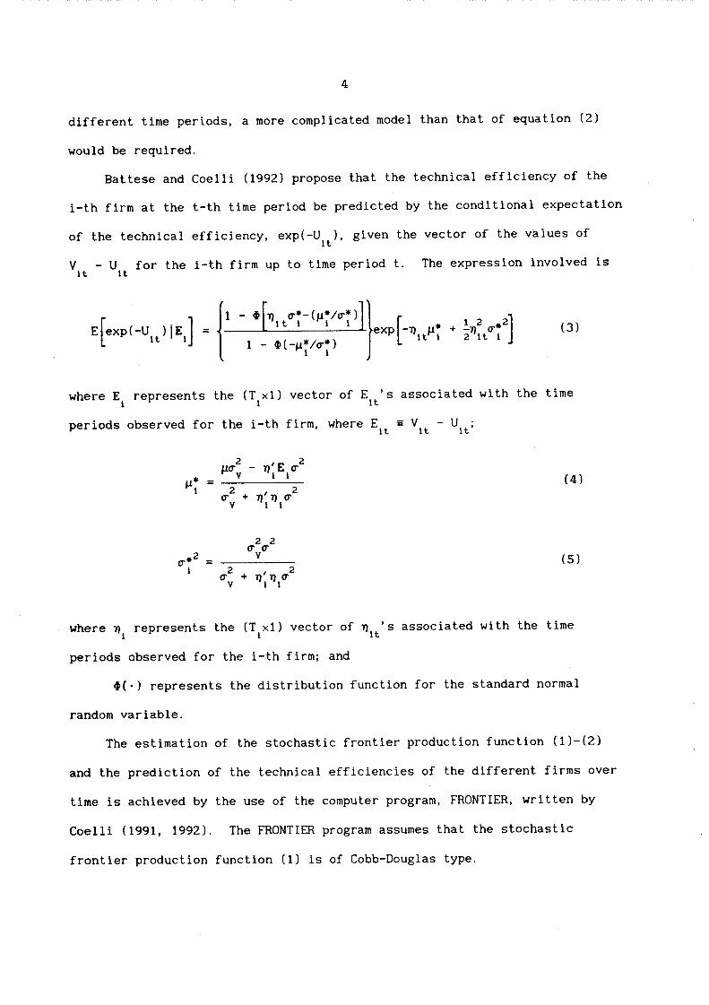
The model proposed by Battese and Coelli (1992) assumes that the

production of firms is defined by a stochastic frontier production function

in which the firm effects are an exponential function of time, such that the

firms are not required to be observed in all the time periods involved. The

model is defined by

and

Y|t = f(x~t;~8)exp(V~. - U~t) (I)

U~t = nltUl : {exp[-n(t-T)]}UI

where t ~ 8(i) and i = 1,2 ..... N;

C2)

Y represents the production for the i-th firm at the t-th period o£it

observat ion;

f(xlt 8) is a function of a vector, xit, o£ factor inputs and other

relevant variables, associated with the production of the i-th firm in the

t-th period of observation, and a vector, 8, of unknown parameters;

the V ’s are assumed to be independent and identically distributedit

N(O, ~a) random errors;

the U’s are assumed to be independent and identically distributed!

non-negative truncations o£ the N(H, ~2) distribution;

~ is an unknown scalar parameter; and

3

~(i) represents the set of T time periods among the T periods involved

for which observations for the i-th firm are obtained. (If the i-th firm was

observed in all T time periods, then ~(i) = {1,2 ..... T}, otherwise ~(i) is a

subset of the set of integers from I to T, which indicate the time periods

for which observations on the i-th firm were obtained.)

The firm effects, Uit, are non-negative random variables which are

associated with the existence of technical inefficiency of the firms. That

is, the observed production, Yit’ is less than the stochastic frontier

production, f(xlt;~)exp(V~ ) for the given set of inputs in the vector, x .

t ’ it

The model for the firm effects, defined by equation (2), specifies that the

firm effects, Ult, approach U1 as t increases towards the last time period,

T, involved in the panel. If the parameter, W, is positive then the firmeffects, Uit, decline towards Ui as t increases towards T. This situation

would indicate a decline in the level of technical inefficiency and, hence,

an increase in technical efficiency over time.

As stated in Battese and Coelli (1992), the exponential specification

of the behaviour of the firm effects over time is a rigid parameterization.

It implies that the technical efficiency of the firms involved,

TEit = exp(-Uit), is a double exponential function of time for the given

firm, i. Kumbhakar (1990) assumed that the firm effects, Uit, were a more

general exponential function of time involving two parameters. No empirical

applications of Kumbhakar’s (1990) model have yet appeared because the model

has not been successfully programmed. Cornwell, Schmidt and Sickles (1990)

assumed that the firm effects were a quadratic function of time in which the

coefficients were random draws from a trivariate normal distribution.

The model for the firm effects, Uit, defined by equation (2), assumes

that the rankings of the firm effects remain the same over time. In order to

permit different orderings of the firm effects, Uit, for the firms at

different time periods, a more complicated model than that of equation (2)

would be required.

Battese and Coelli (1992) propose that the technical efficiency of the

i-th firm at the t-th time period be predicted by the conditional expectation

of the technical efficiency, exp(-Uit), given the vector of the values of

V - U for the i-th firm up to time period t. The expression involved is~t

C3)

where EI represents the (TI×I) vector of Eit s associated with the time

--V -U ¯periods observed for the i-th firm, where Eit it it’

2 2

(4)

2 2O" O"

o.*2 (5)i °’2v + ~i°’2

where nI represents the (Tixl) vector of nlt s associated with the time

periods observed for the i-th firm; and

#(.) represents the distribution function for the standard normal

random variable.

The estimation of the stochastic frontier production function (I)-(2)

and the prediction of the technical efficiencies of the different firms over

time is achieved by the use of the computer program, FRONTIER, written by

Coelli (1991, 1992). The FRONTIER program assumes that the stochastic

frontier production function (I) is of Cobb-Douglas type.

Battese and Coelli (1992) illustrated the use of the FRONTIER program

with the analysis of a subset of the data on a panel of sample farms from the

village of Aurepalle in India. In this paper, we consider the complete data

sets obtained over the ten-year period in which ICRISAT collected data from

the three villages of Aurepalle, Kanzara and Shirapur.

3. ICRISAT’s Village Level Studies

The data used in this study were obtained from the International Crops

Research Institute for the Semi-Arid Tropics (ICRISAT) near Hyderabad in the

Indian state of Andhra Pradesh. The data are from the village level studies

(VLS) in which ICRISAT personnel collected a range of data from households

engaged in agricultural production in different villages in India. As a part

of its mandate, ICRISAT initiated its village level studies in 1975 to obtain

reliable data on traditional agricultural methods in the Semi-Arid Tropics

(SAT) of India so that improved technological methods could be introduced

[see 3odha, Asokan and Ryan (1977) and Binswanger and 3odha (1978)].

The three villages involved in the VLS studies of ICRISAT were selected

from districts which represented the broad agroclimatic subregions in the SAT

of India. The main factors considered in the selection of the districts

included soil types, rainfall and cropping pattern. Accessibility to

agricultural universities or research stations and development programs and

proximity to the ICRISAT’s headquarters at Patancheru near Hyderabad were

also given important consideration. Within the selected districts, talukas

(subdivisions of a district) were selected which represented the typical

characteristics in terms of land-use pattern, cropping, irrigation,

livestock, infra-structural development, population, etc. Villages which

were located near large towns or have special government or other programs

were not considered in the sample. The data used in this study were

collected from three villages, Aurepalle, Shirapur and Kanzara, during the

years 1975-76 to 1984-85. Data on factor inputs and total production were

obtained for a random sample of households in each village.

All households in each village were divided into two main groups. The

agricultural labour group consisted of households operating less than 0.2

hectares of land and the cultivator group consisted of households operating

at least 0.2 hectares of land. The cultivator group was further classified

into three equal groups and ranked as small, medium and large farmers

depending on the size of their holdings.

A random sample of ten households was selected from each group of

farmers including the agricultural labour group so that 40 sample farmers

were selected from each village. However, this study does not include the

agricultural labour group for the purpose of the analysis of the frontier

production function. During the ten-year period involved, some households

which were originally classified as labour farmers became small farmers in

the later years and hence were included in the sample. Farmers who refused

to provide information or ceased to be members of the sample were replaced by

other farmers. Hence the numbers of sample households in each village, as

well as the number of time-series observations for each household, were not

necessarily equal.

The villages of Aurepalle, Shirapur and Kanzara were selected from the

districts of Mahbubnagar, Sholapur and Akola, respectively, and are located

approximately 70 km south, 336 km west and 550 km north of Hyderabad,

respectively. There were 3141 people in Aurepalle, 2017 people in Shirapur

and 1380 people in Kanzara in 1985.

Considerable soil heterogeneity is a characteristic of the SAT of India.

Aurepalle has medium and shallow alfisols (red soils) with low water

retention capacity. Soil heterogeneity is remarkably high in Aurepalle

compared with Shirapur and Kanzara. Shirapur has medium and deep vertisols

(black soils) with high moisture retention capacity. Kanzara has mainly

medium-deep black soils and shallow vertisols with medium moisture retention

capacity. Soils in Kanzara are more homogeneous than in Aurepalle and

Shirapur.

Rainfall in the SAT of India is generally erratic in distribution and

the mean annual rainfall ranges from about 400 mm to 1200 mm. In the years

197S to 1985 the average annual rainfall was 611 mm for Aurepalle, 629 mm

for Shirapur and 8S0 mm for Kanzara. Rainfall is very erratic and uncertain

in Aurepalle and Shirapur.

Walker and Ryan (1990) report that during four years of the study period

Aurepalle and Shirapur had very little rainfall. Rainfall is relatively

higher and less variable in Kanzara. Agriculture is predominantly dryland

with two main seasons, the rainy season (kharif) which spans the months of

June to October followed by the post-rainy (rabi) season.

In Aurepalle, dryland crops include sorghum, pearl millet, pigeonpea,

castor and high-yielding variety (HYV) paddy. Sorghum, pearl millet,

pigeonpea are intercropped, usually with one row of pigeonpea to four rows of

cereal crops. The high-yielding variety paddy is mostly grown under

irrigated conditions. Of the total cropped land, about 21 per cent is

irrigated in Aurepalle, compared with 9 per cent and 7 per cent in the

villages of Shirapur and Kanzara, respectively.

The rabi season has more reliable rainfall in the village of Shirapur.

During the rabi season farmers grow mainly sorghum and chickpea. Local wheat

and safflower are also grown. Irrigation is used for onions, chillies and

other vegetables. However, the use of high-yielding varieties is very

limited in Shirapur.

The village of Kanzara has relatively favourable rainfall in the kharif

season and the crops grown include cotton, pigeonpea, hybrid sorghum, local

sorghum, groundnut, green gram and black gram. Wheat and chickpea are mainly

planted in the rabi season. Intercropping is more prevalent in Kanzara than

in the other two villages. The use of improved technology, such as

high-yielding varieties of sorghum and cotton, fertilizers and pesticides, is

also high in Kanzara compared with the villages of Aurepalle and Shirapur.

There exists a large variation in the cropping patterns among the three

villages. This variation is associated with differences in soil

heterogeneity, rainfall pattern and other factors among the villages.

Shirapur has the highest proportion of area cropped under cereals, of which

local sorghum contributes about 62 per cent of the total cultivated land in

the village. The area under cereals in Aurepalle and Kanzara is about 50 and

30 per cent respectively. Oil crops play an important role in Aurepalle,

where castor contributes about 35 per cent of the total cropped land,

followed by sorghum and paddy which contribute about 20 per cent each.

Cotton is a sole crop in Kanzara. It occupies about 40 per cent of the

cultivated land in the village.

A similar variation exists in the marketed output of crops in the three

villages. The crops which have the largest proportion of marketed output are

castor in Aurepalle, cotton in Kanzara and sunflower in Shirapur. The cereal

crops, sorghum, pearlmillet, paddy and wheat, are mainly subsistence crops.

The labour market includes cultivators and agricultural labourers who

comprise about two-thirds of the active workers in SAT India. The labour

market is active in the three villages. However, the use of labour (family

and hired) varies from village to village, as well as from year to year,

depending on rainfall, soil type, type of crop, irrigation, etc. Farm

households depend heavily on hired labour to cultivate their land. In

Aurepalle and Kanzara, hired labour provides the majority (60 to 80 per cent)

of the total labour used in crop production. The high demand for hired

labour is due to the activities of paddy transplanting in Aurepalle and

cotton picking in Kanzara [see Walker and Ryan {1990)]. The labour force

comprises men, women and children, but the latter only make a very small

contribution. The contribution of men to the total family labour in crop

production is substantially higher than women, while women dominate the hired

labour market.

In all the villages, cultivation such as plowing, harrowing and

interculturing is carried out using animal draft power, usually involving

bullocks. However, many households which own small areas of land do not have

bullocks. Seasonal hiring is common, especially by small farmers. It is

most common in Shirapur where bullock-to-land ratios are significantly lower

than in the other two villages [Walker and Ryan (1990}]. Single bullock

owners often pool their bullocks and cultivate on an exchange basis.

Fertilizer is used almost entirely for irrigated agriculture in the

study villages. However, the use of fertilizer in dryland agriculture is

increasing in the rainfall-assured village of Kanzara and, to some extent, in

Aurepalle. For example, the use of fertilizer in dryland farming has

increased from 3 per cent in 1975-76 to 50 per cent by 1985-86. However,

application rates per hectare remained very low.

Manure plays an important role in the study villages. Many farmers

apply manure to their land every year. However, the supply of manure is

constrained by limited availability of fodder which restricts livestock

production as well as its use for fuel.

Pesticides are applied mainly in irrigated agriculture, although the

expenditure on fertilizers is much higher (about nine times) than the

expenditure on pesticides. Pesticides are widely applied in the villages of

10

Aurepalle and Kanzara.

The following section deals with the empirical analyses of the data

obtained from the three villages, Aurepalle, Shirapur and Kanzara. It is

expected that different parameter values and technical efficiencies are

likely because of the substantial differences in the agro-climatic

environments among the three villages.

4. The Frontier Production Function

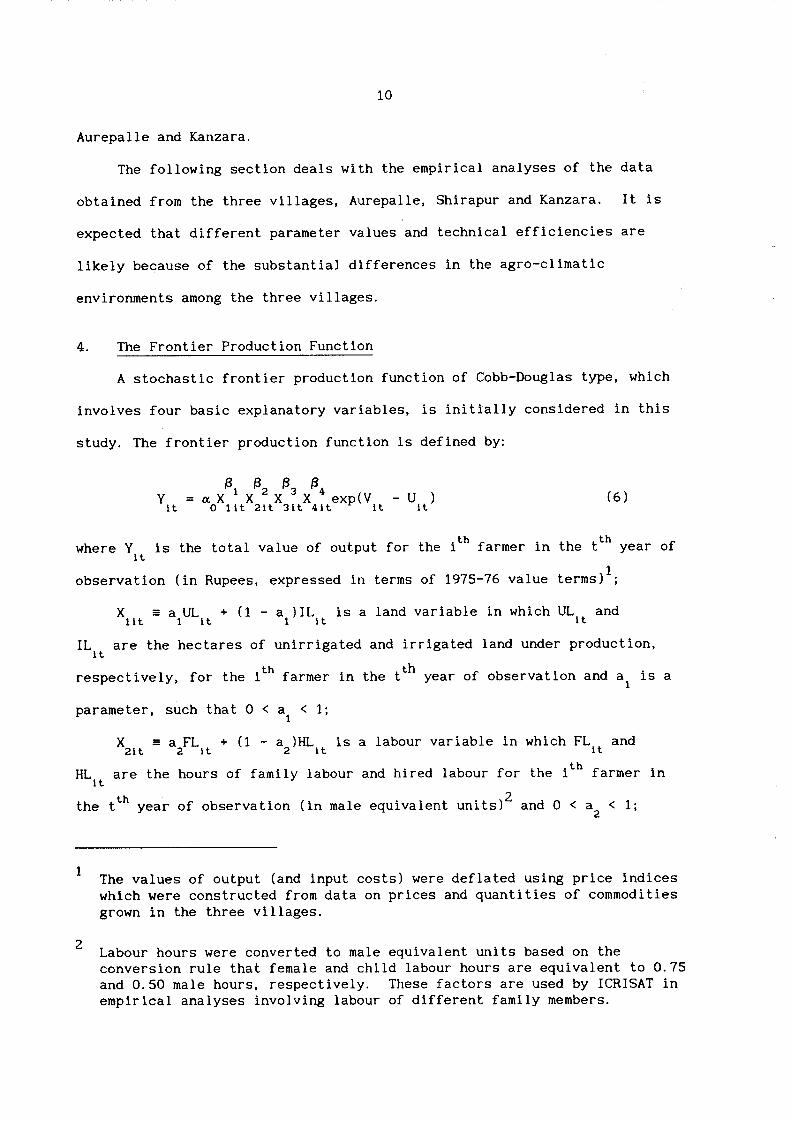
A stochastic frontier production function of Cobb-Douglas type, which

involves four basic explanatory variables, is initially considered in this

study. The frontier production function is defined by:

~! X~2 X~3 X~4 ) (6)= ~ X exp(Vlt - UYit 0 lit 2it 3it 4it it

where Y is the total value of output for the ith farmer in the tth year ofit

1observation (in Rupees, expressed in terms of 1975-76 value terms) ;

X = a UL + (1 - a )IL is a land variable in which UL andllt I it 1 it it

IL are the hectares of unirrigated and irrigated land under production,itrespectively, for the ith farmer in the tth year of observation and a1 is a

parameter, such that 0 < aI < 1;

X21t = a2FLit + (1 - a2)HLit is a labour variable in which FLit and

HL are the hours of family labour and hired labour for the ith farmer inItthe tth year of observation (in male equivalent units)2 and 0 < a2 < I;

2

The values of output (and input costs) were deflated using price indiceswhich were constructed from data on prices and quantities of commoditiesgrown in the three villages.

Labour hours were converted to male equivalent units based on theconversion rule that female and child labour hours are equivalent to 0.75and 0.50 male hours, respectively. These factors are used by ICRISAT inempirical analyses involving labour of different family members.

11

X = OB + HB m Bullock is the bullock labour variable in which3it it it it

OB and HB represent the hours of owned and hired bullock labour (init it

pairs), respectively, for the ith farmer in the tth year of observation;

X m exp(Cost ) is the exponent (or anti-logarithm) of the total cost41t it

of inputs (involving inorganic fertilizer, organic matter applied to land,

pesticides and machinery costs) for the ith farmer in the tth year of

observation;

~o’ 81’ 62’ 83 and 84 are parameters to be estimated; and

V and U are random variables having the distributional properties,it it

as defined for equations (I) and

The model, defined by equation (6), is formulated from the work of

Bardhan (1973), Deolalikar and ViOverberg (1983, 1987) and Battese, Coelli

and Colby (1989). Bardhan (1973) considered a production function of

Cobb-Douglas type in which the variables, total labour (family plus hired

labour hours) and the proportion of hired labour to total labour, were

separately included as explanatory variables. Bardhan (1973) used Indian

farm-level data and concluded that hired and family labour were

heterogeneous in some cases.

Deolalikar and Vi3verberg (1983) defined a more general model of CES

type in the analysis of district-level data for Indian farms. Several

special cases of the CE$ model were considered. They concluded that the

model in which hired and family labour were included as separate explanatory

variables was the best one. Deolalikar and Vi3verberg (1983) also considered

unirrigated and irrigated land in their production function. They concluded

that the best model had a weighted average of the unirrigated and irrigated

areas operated as the land variable.

Battese, Coelli and Colby (1989) considered the model in which labour

and land variables were the weighted averages of their respective hired and

12

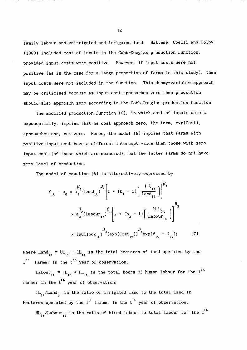
family labour and unirrigated and irrigated land. Battese, Coelli and Colby

(1989) included cost of inputs in the Cobb-Douglas production function,

provided input costs were positive. However, if input costs were not

positive (as is the case for a large proportion of farms in this study), then

input costs were not included in the function. This dummy-variable approach

may be criticised because as input cost approaches zero then production

should also approach zero according to the Cobb-Douglas production function.

The modified production function (6), in which cost of inputs enters

exponentially, implies that as cost approach zero, the term, exp(Cost),

approaches one, not zero. Hence, the model (6) implies that farms with

positive input cost have a different intercept value than those with zero

input cost (of those which are measured), but the latter farms do not have

zero level of production.

The model of equation (6) is alternatively expressed by

Y = ~ x a (Landit 0 1 it

~1 [

/ I L~t

) 1 + (b1 - 1) Landit

~2

x a (Labour )

1 + (b2 - 1) Labour

2 it it

t93/34exp (Vit

x (Bullockit) [exp(Costlt)] - Ult);(7)

where Land -= UL + IL is the total hectares of land operated by theit it it

thi farmer in the tth year of observation;

.thLabour = FL + HL is the total hours of human labour for the I

It it it

farmer in the tth year of observation;

IL /Land is the ratio of irrigated land to the total land init it

hectares operated by the ith farmer in the tth year of observation;

thHL /Labour is the ratio of hired labour to total labour for the i

it it

13

farmer in the tth year of observation; and

b and b are parameters defined by1 2

bI ~ (I - al )/al and b2 ~ (I - a2)/a2.

It is noted that if unirrigated and irrigated land were equally

productive (an unlikely occurrence) then the parameter, a1, would be 0.5,

which implies that the parameter, bl, would be equal to 1.0. Similarly, if

hired and family labour were equally productive, then the parameter, b2,

would be equal to 1.0.

We, in fact, estimate a linearized version of the model of equation (7),

obtained by considering the first-term of the Taylor expansion for the land

and labour variables, namely

log Yit = Ho + 811og(Landit) + 821og(Labourit) + 831og(Bullockit)

I Lit + 82(b2-1) Labour

+ 81(b1-1) Land+ SaC°stir it

+ v - uit it

The parameter, 80’ is a simple function of a0’ 8~, a~, 82 and a2.

It should be noted that the model of equation (8) is not equivalent to

that of equations (6) or (7). The function (8) would be a close

approximation to that of equation (7) if the land- and labour-ratio variables

had values which were close to zero.

If hired and family labour were equally productive , then the

coefficient of the labour-ratio variable, HLit/Lab°urit’ would be zero. Thus

testing that the coefficient of the labour-ratio variable is zero provides a

procedure for testing whether hired and family labour are equally productive

in the villages involved.

14

5. Empirical Results

A summary of the data on the different variables in the frontier

production function is given in Table I. It is evident from these statistics

that Aurepalle farmers tend to be smaller in terms of value of output and

total land operated. Kanzara farmers had the highest mean value of output,

human labour and bullock labour. Kanzara farmers have the least amount of

irrigation because of the relatively assured rainfall, whereas Aurepalle

farmers have the greatest amount of irrigation because of the prevalence of

growing paddy.

Bullock labour is used considerably more in Kanzara and Aurepalle than

in Shirapur. Cost of inputs had a high proportion of zero observations in

all three villages and so the sample means were not very large in all three

cases.

The stochastic frontier production function (8) consists of ten

parameters, six being associated with the explanatory variables of the

function and four being parameters which specify the distributions of the

random variables, Vlt and Uit. The maximum-likelihood estimates for the

parameters of the frontier production functions with time-invariant

parameters for the three villages are presented in Table 2.

Tests of hypotheses about the distribution of the random variables

associated with the existence of technical inefficiency and residual error

are of interest. The frontier production function is equivalent to the

traditional response function if the parameters, ~, ~ and ~, are

simultaneously equal to zero. Hence a test of the null hypothesis,

H : ~=n=~=O, is desirable. Further, if the parameter, n, was zero, then theo

farm effects associated with the existence of technical inefficiency would be

time invariant. Also, if the parameter, ~, was zero, then the farm effects

associated with the last period of observation in the panel would have

15

Table 1. Summary Statistics for Variables in the Stochastic

Frontier Production Function for Farmers in Aurepalle,

ShirapuF and Kanzara

Variable

Sample Sample Standard Minimum Maximum

Mean Deviation Value Value

Value of Output (Rs, in 1975-76 values)

- Aurepalle- Shirapur- Kanzara

3,559.93,689.15,206.7

4,482.73,437.27,207.7

Land (hectares)

- Aurepalle- Shirapur- Kanzara

4.236.635.99

3.805.457.38

Land Ratio, IL/Land

- Aurepalle- Shirapur- Kanzara

0.140.13O. 06

0.210.240.13

Human Labour (hours)

- Aurepalle- Shirapur- Kanzara

2,133.51,658.92,565.7

2,697.41,558.63,138.7

Labour Ratio, HL/Labour

- Aurepalle- Shirapur- Kanzara

O, 42O. 45O, 56

O. 29O. 20O. 27

7.222.0

121.6

0.160.610.40

000

184058

00.060.016

18,09426,42339,168

20.9724.1936.34

1.01.01.0

12,91611,14615,814

0.980.980.996

Bullock Labour

- Aurepalle- Shirapur- Kanzara

518.9340.6567.3

592.8280.5763.5

81412

4,3161,2403,913

Cost of Inputs

- Aurepalle- Shirapur- Kanzara

626.4458.8626.0

963.31,023.8

975.8

000

6,2056.7465.344

16

Table 2: Maximum-likelihood Estimates for Parameters of Stochastic

Frontier Production Functions with Time-Invariant Coefficients for

Farmers in Aurepalle, Shirapur and Kanzara

M.L. Estimates for Production Frontiers in

Variable Parameter Aurepalle Shirapur Kanzara

Constant

8°1.47 2.81 1.62

(0.58) (0.52) (0.66)

Log(Land) 81 0.36 0.183 0.102(0.11) (0.061) (0.079)

Log(Labour) 82 1.27 0.781 0.836

(0.12) (0.086) (0.096)

Log(Bullocks)

8a-0.557 -0.104 0.049(0.069) (0.054) (0.064)

Cost 84 0.00011 0.00123 0.00387

(0.00099) (0.00073) (0.00075)

IL/Land85 m 81 (~ -1)

0.38 -0.11 0.44(0.29) (0.13) (0.20)

HL/Labour86 m 82{~-I)

-0.28 0.12 -0.16(0.12) (0.13) (0.11)

0.248 0.324 0.132(0.073) (0.044) (0.012)

0.30 0.638 0.146(0.21) (0.029) (0.052)

0.19 0.269 0.011(0.22) (0.062) (0.024)

-0.89 -2.87 0.46(0.99) (0.92) (0.38)

Loglikelihood -172.06 -131.18 -111.24

The estimated standard errors for the maximum-likelihood estimates are

presented below the corresponding estimates. These values are generated

by the computer program, FRONTIER.

17

half-normal distribution. Hence the null hypotheses that ~ and N are zero,

either simultaneously or individually, are of interest if the stochastic

frontier function is significantly different from the traditional response

function. Statistics required for testing these various hypotheses

associated with the parameters, ~, n and N, are presented in Table 3. The

generalized likelihood-ratio test statistic is calculated after obtaining the

logarithm of the likelihood function associated with the restricted maximum-

likelihood estimates for the special cases when the appropriate parameters

are zero. The last column of Table 3 gives the probability of exceeding the

2calculated X -value if the respective null hypothesis is true. This value is

called the "prob-value" and the null hypothesis is rejected if the prob-value

is smaller than the desired value for the probability of a Type I error.

The results presented in Table 3 imply that, given the specifications of

the stochastic frontier production function (8) with time-invariant

parameters, then the model is significantly different from the traditional

response function for all three villages. Further, for farmers in Aurepalle

and Shirapur no sub-model in which the parameters, W and N, are zero, either

jointly or individually, is an adequate representation of the data. That is,

technical inefficiency not only exists, but the farm effects are not time

invariant, nor is the half-normal distribution an adequate representation.

However, for farmers in Kanzara, the null hypothesis that the farm effects

are time invariant and have half-normal distributions would be accepted

under the model assumptions, given that the desired probability of a Type I

error was no larger than O. lO.

The above model for the stochastic frontier production function

associated with panel data on sample farmers from the three villages is

likely to be inappropriate. That is, the assumption that the coefficients of

the explanatory variables in the frontier function (8) are time invariant,

18

Table 3: Statistics for Tests of Hypotheses for Parameters of the

Distribution of the Farm Effects, Uit, Associated with the

Stochastic Frontier Production Function with Time-Invariant Coefficients

for the Farmers in Aurepalle, Shirapur and Kanzara

Null Hypotheses Loglikelihood X2-value m c

Prob-Value m p

p(xZ > C[Ho true)

H: ~=n=~=O0

Aurepalle

Shirapur

Kanzara

-180.65

-210.80

-119.01

17.18

159.24

15.54

p < O. 005

p < O. 005

p < 0. 005

H: ~=~=0o

Aurepalle

Shirapur

Kanzara

-179.43

-196.62

-113.48

14.74

130.88

4.48

p < O. 005

p < O. 005

p > 0.10

H: D=0o

Aurepalle

Shirapur

Kanzara

-178.92

-194.89

-111.56

13.72

127.42

0.64

p < 0. 005

p < 0. 005

p > 0. I0

H: ~=0o

Aurepalle

Shirapur

Kanzara

-175.19

-138.35

-113.12

6.26

14.34

3.76

0.010 < p < 0.025

p < 0. 005

0.05 < p < 0. I0

19

but that the farm effects associated with technical inefficiency have a

particular time-varying structure may be regarded as objectionable. Hence we

now consider a modification of the model in which the coefficients of the

explanatory variables in the frontier production function are time varying

and are, in fact, a linear function of the year of observation. That is, we

consider the stochastic frontier production function, defined by

log Yit = ~ot + ~It l°g(Landlt) + /~2t l°g(Lab°urlt)

+ ~3t l°g(Bull°cklt) + ~4tC°stlt

/Landlt) + ~6t(HL /Labour ) + V - U (9)+ ~85t ( ILit it it it it

where

~Jt = ~J + 6.(Year] It) m ~j + 6j×t’ j = 0, I .....6. (I0)

For this more general specification o£ the stochastic frontier

production function, there would be interest in testing if the coefficients

of the production frontier were time invariant, or the elasticities with

respect to the factor inputs were time invariant, after investigating whether

the farm effects were time invariant and/or the half-normal distribution was

a reasonable assumption.

The maximum-likelihood estimates for the parameters of the stochastic

frontier model (9)-(10) with time-varying parameters and time-varying farm

effects (2) are presented in Table 4. Tests of hypotheses about the

distribution of the farm effects associated with the stochastic frontier

production functions with time-varying coefficients are obtained from the

data in Table 5.

The statistics in Table 5 suggest that, given the specifications of the

stochastic frontier production function with time-varying coefficients and

time-varying technical inefficiencies (9)-(I0):

2O

Table 4: Maximum-likelihood Estimates for Parameters of the Stochastic

Frontier Production Functions with Time-Varying Coefficients

for Farmers in Aurepalle, Shirapur and Kanzara

M,L. Estimates for Production Frontiers inVariable Parameter Aurepalle Shirapur Kanzara

Constant ~o

Year ~ o

Log(Land) ~I

2.16 3.02 3.11(0.86) (0.86) (0.96)

-0. 21 -0.21 -0.1013) (0.13) (0.89)

47 0.29 0.4018) (0.14) (0.68)

Year x Log(Land)

Log(Labour)

Year x Log(Labour)

Log(Bullock)

Year x Log(Bullock)

Cost

-0.041(0 034)

-0.033 -0.03(0.026) (0.54)

Year x Cost

1.14(0 23)

0.62 0.73(0.12) (0.68)

IL/Land ~s

-0.055(0 043)

0.043 -0.001(0.022) (0.87)

Year x (IL/Land) ~ 5

-0.57(o 22)

-0,06 -0. I0(0.14) (0.54)

HL/Labour ~6

-0.003(0 047)

-0.007 0.02(0.022) (0.19)

0.16(o 12)

-0.28 0.79(0.16) (0.71)

-0. 16(o 12)

0.28 -0.76(0.16) (0.71)

0.84 0.51 0.94(0.66) (0.31) (0.87)

-0.16 -0.127 -0.07(0.12) (0,049) (3.5)

-0.56 0.61 -0.35(0.19) (0.28) (0.99)

Year x (HL/Labour) &6

C.043 -0.077 0.05(0.032) (0.045) (2.5)

0.270 0.146 0.11(0.032) (0.028) (0.59)

~ = ¢2/~2 0.37 0.21 0.26s

(0.19) (0.13) (0.72)

-0.10 0.226 0.002(0.10) (0.061) (8.6)

-0.49 -0.22 0.59(0.75) (0.15) (1.7)

Loglikelihood -158.07 -121.87 -74.53

21

Table 5: Statistics for Tests of Hypotheses for Parameters of the

Distribution of the Farm Effects, Uit, Associated with theStochastic Frontier Production Function with Time-Varying Coefficients

for the Farmers in Aurepalle, Shirapur and Kanzara

Null Hypotheses Loglikelihood X2-value ~ c

Prob-Value m pP(X2 > cIH° true)

Aurepalle -159.54 2.94 p > 0. I0

Shirapur -166.69 44.82 p < 0.005

Kanzara -90.69 32.32 p < 0.005

H: D=~=Oo

Aurepalle -159.09 2.04 p > 0. I0

Shirapur -142.86 41.98 p < 0.005

Kanzara -77.59 6.12 0.025 < p < 0.05

H: D=Oo

Aurepalle -158.36 0.58 p > 0. I0

Shirapur -141.69 39.64 p < 0.005

Kanzara -74.57 0.06 p > 0. I0

H: ~=0o

Aurepalle

Shirapur

Kanzara

-159.10

-139.94

-77.63

2.06

35.94

6.20

p > 0.10

p < O. 005

0.01 < p < 0.025

(i) For Aurepalle farmers, the hypothesis that the traditional response

function is an adequate representation of the data would not be rejected,

given that the desired probability of a Type I error was not greater than

0. I0. Hence it could be concluded that technical inefficiency is not evident

for Aurepalle farmers.

(ii) For Shirapur farmers, the null hypotheses, that the traditional

response function is an adequate representation, or that the farm effects

associated with technical inefficiency are time invariant and/or have

half-normal distribution, would be rejected, given that the probability of a

Type I error was not larger than 0. i0.

(iii) For Kanzara farmers, the null hypothesis that the technical

inefficiencies of farmers were time invariant would not be rejected by the

data.

Given these conclusions about the time-varying nature of the technical

inefficiencies of farmers (when present) in the stochastic frontier

production functions, various null hypotheses about the coefficients of the

frontiers for the three villages are considered. The relevant test

statistics are presented in Table 6 for three particular null hypotheses.

The first null hypothesis, H : 6 = 6 = ... = ~ = O, implies that the0 0 1 6

stochastic frontier production function (9) is equivalent to model (8), which

has time-invariant coefficients. This hypothesis is rejected for all three

villages.

The second null hypothesis, H : 6 = 6 = ... = 6 = O, specifies that0 I ~ 6

the coefficients of the explanatory variables in the production frontier are

time invariant, but that the model accounts for neutral technological change.

This null hypothesis would be rejected for Shirapur and Kanzara if the

desired probability of a Type I error was 0.01.

23

Table 6: Statistics for Tests of Hypotheses for Coefficients of the

Explanatory Variables of the Appropriate Stochastic Frontier

Production Functions for Farmers in Aurepalle, Shirapur and Kanzara

Null Hypotheses LoglikelihoodI

Prob-Value ~ p~2-value ~ c P(~2 > clH° true)

H : 6 = 6 = ... = 6 = 0O O 1 6

Aurepalle -172.06 25.04 p < 0.005

Shirapur -131.18 18.62 0.005 < p < 0.01

Kanzara -113.48 77.82 p < 0.005

H : 6 = 6 = ... = 6 = 00 1 2 6

Aurepalle -166.02 12.96 0.025 < p < 0.05

Shirapur -130.77 17.80 0.005 < p < 0.01

Kanzara -113.30 77.46 p < 0.005

=6 =0Ho: ~6 6

Aurepalle -164.57 10.06 0.005 < p < 0.01

Shirapur -130.89 18.04 p < 0.005

Kanzara -76.45 3.76 p > 0.10

The loglikelihood values are calculated assuming that the stochastic

frontier production functions for the three villages have ~=~=p=O for

Aurepalle; ~, ~ and p are free parameters for Shirapur; and ~=0 for

Kanzara.

24

= = O, implies that the labourThe third null hypothesis, Ho: ~6 66

ratio variable, HL/Labour, is absent from the model because hired and family

labour are equally productive. This hypothesis would be rejected for

Aurepalle and Kanzara, if the probability of a Type I error was 0.01.

On the basis of the above tests of hypotheses, we conclude that the

preferred models for the three villages are:

(i) For Aurepalle: the traditional response function in which the

coefficients of the explanatory variables are time invariant, but year of

observation is included to account for technological change;

(ii) For Shirapur: the stochastic frontier production function with

time-varying technical inefficiency and time-varying coefficients for the

explanatory variables;

(iii) For Kanzara: the stochastic frontier production function with

time-invariant technical inefficiency but time-varying coefficients of the

explanatory variables, such that family and hired labour are equally

productive.

Given the specifications of the stochastic frontier production functions

with time-varying parameters and technical efficiencies which are considered

in this paper, the estimated parameters for the preferred frontier models are

presented in Table 7. Since farmers in Shirapur have time-varying technical

efficiencies, predictions for the technical efficiencies of the sample

farmers in the years of observations are presented in Table 8. The technical

efficiencies of Shirapur farmers in the first year of observation showed

great variability (from 0.191 to 0.898) but increased over the ten-year

period to as high as 0.985. However, predictions for the time-invariant

technical efficiencies of the Kanzara farmers, presented in Table 9, varied

from 0.466 to 0.818. In both cases, the level of technical inefficiency of

the farmers involved was considerable for most farmers.

25

Table 7: Maximum-likelihood Estimates for Parameters of the Preferred

Stochastic Frontier Production Functions with Time-Varying

Coefficients for Farmers in Aurepalle, Shirapur and Kanzara

M.L. Estimates for Production Frontiers inVariable Parameter Aurepalle Shirapur Kanzara

Constant 8o 0.50 3.02 3.24(0.41) (0.86) (I.03)

Year 6 0.0545 -0.21 0.07o (0.0099) (0.13) (0.14)

Log(Land) 81 0.289 0.29 0.40(0.086) (0.14) (0.14)

Year x Log(Land) 6 0 -0.033 -0.0321 (0.026) (0.023)

Log(Labour) 82 1.434 0.62 0.66(0.095) (0.12) (0.17)

Year x Log(Labour) 6 0 0.043 -0.0092 (0.022) (0.028)

Log(Bullock) 83 -0.619 -0.06 -0.07(0.074) (0.14) (0.14)

Year x Log(Bullock) ~ 0 -0.007 0.0173 (0.022) (0.023)

Cost 84 -0.00040 -0.28 0.729(0.00097) (0.16) (0.085)

Year x Cost 6 0 0.28 -0.7254 (0.16) (0.085)

IL/Land 8s 0.03 0.51 0.84(0.23) (0.31) (0.46)

Year x (IL/Land) 6 0 -0.127 -0.059s

(0.049) (0.056)

HL/Labour 86 -0.36 0.61(0.11) (0.28)

Year x (HL/Labour) 6 0 -0.0776 (0.045)

2 2 2¢ -= ~ + 0~ 0.191 0.146

S V

¯ ~, ~ 0.,2/0‘2S

0.112(0.028) (0.012)

0.21 0.242(0.13) (0.071)

O.226 0(0.061)

-0.22 0.56(0.15) (0.64)

Loglikelihood -166.02 -121.87 -76.45

26

Table 8: Predicted Technical Efficiencies of

Shirapur Farmers from 1975-76 to 1984-851

Technical Efficiencies

Farmer 75-76 76-77 77-78 78-79 79-80 80-81 81-82 82-83 83-84 84-85

2 -3 -4 -5 3096 7907 6908 2659 351

10 53311 63212 90813 57214 73815 55416 48817 522

18 53919 60520 89421 38322 81823 19124 63725 80126 53027 89828 76029 68630 85831 90932 53833 -34 -35 -36 -37 -38 -

¯ 585¯ 242¯ 859

¯ 390¯ 827¯ 742¯ 346

604691925638783622563593609668914

¯ 851

6̄958366019178O2739884926

¯ 345

.719

¯ 871

¯ 650¯ 321¯ 885

¯ 471¯ 859¯ 786¯ 428

667743940698821683631658671723930

¯ 879

¯7478666649338377849O5940

¯ 426

¯ 767

¯ 895

¯ 708¯ 403¯ 906

¯ 548¯ 885¯ 824¯ 507

¯ 723¯ 788

749853737691715727771943609901

791891721946867822923

¯ 758¯ 484¯ 924

618907857581255771827

794881784744765775812954

¯ 920¯ 505¯ 829.912¯ 770

¯ 892¯ 855¯ 938

¯ 8Ol

¯ 939¯ 807¯ 681¯ 924

.648¯ 336.812¯ 859

8319038237908O7815847963728935

861929811965920882

¯ 868

¯ 960¯ 871¯ 783¯ 951

¯ 759¯ 499¯ 876¯ 907

¯ 889¯ 937¯ 883¯ 860

¯ 878¯ 899

.816¯ 958

908954875977943923

¯ 837

¯ 951¯ 842¯ 736¯ 939

¯ 788¯ 419

¯ 885

¯ 863¯ 922¯ 856¯ 828

¯ 849¯ 875¯ 971¯ 776¯ 948

887942846972929905

.812

¯ 955

¯ 893

¯ 968¯ 895¯ 822¯ 961

¯ 802¯ 574¯ 899¯ 925

¯910¯ 949¯ 905

¯ 901¯ 918

¯ 850¯ 966

926963899982954938

.505 .579 .646 - -- - .781 .852 .879

.808 ¯842 - .916 .932- - - .897 .916

.914 .931 .944 .964 .971

Mean .592 .647 .699 .745 .787 .823 .854 .881 .903 .921

.913

¯ 974¯ 915

¯ 968

¯ 839¯ 642.919¯ 940

¯ 927

¯ 924

¯ 920¯ 934

¯ 878¯ 973

94197091898596395O

¯ 902¯ 945.932.977¯ 929

1Values of technical efficiencies are not obtained in years when no

observations are observed¯

27

Table 9: Predicted Technical Efficiencies of Kanzara Farmers

Farmer Technical Efficiency

123456789

101112131415161718192O212223242526272829303132333435

0.5110.4830.5910.5500.5570.5230,6060.4920.6360.6840.6510.5660.6050.4680.6580.5010,5130.7020.4720.5730 5050 5410 4790 5580 7590 4660.5300.8180.5980.5120.6090.6000.6520.5530.597

Mean 0.575

It is noted that the coefficient of the logarithm of Bullock labour in

the preferred production frontiers have negative values for all three

villages, but the coefficient is significantly different from zero in

Aurepalle only. Negative elasticities of bullock labour have been found in

other studies [e.g., Saini (1979), Battese, Coelli and Colby (1989) and

Battese and Coelli (1992)]. Various explanations have been suggested for

this phenomenon.

5. Conclusions

Our application of frontier production functions in the analysis of

panel data from three Indian villages has indicated a number of important

findings:

(i) When the data are analysed using a frontier model with coefficients

that are constant over time (including the intercept parameter), then

technical inefficiencies are found to be highly significant in all three

villages and to be time varying in two of the three villages;

(ii) If the frontier production function contains time-varying

coefficients (intercept and elasticities) then different conclusions about

technical inefficiency were obtained in the different villages. In

Aurepalle, the frontier function was not significantly different from the

traditional response function (which can be estimated efficiently by ordinary

least-squares regression). In Kanzara technical inefficiency was not

significantly different over time. However, in Shirapur it could not be

concluded that technical efficiency was time invariant for the farmers

involved.

(iii) The hypothesis that the coefficients of the explanatory variables

(other than the intercept) were time invariant was rejected for two of the

29

three villages.

The above results indicate that the inclusion of year-of-observation as

an explanatory variable in the frontier model to account for neutral

technological change, provided that it is appropriate, does not necessarily

imply that technical inefficiency will then be absent from the model, as was

found in the empirical example reported by Battese and Coelli (1992).

Our analysis of the farm-level data from the three villages has not

proceeded to the point of being able to explain or justify the different

results which have been obtained for the three villages. Further

investigations are required to deal with such issues.

The application of the frontier production function models considered in

this paper has not included the possible effect of farm- or farmer-specific

variables, such as education of the farmer, access to credit, etc. Further

analyses incorporating such variables in the frontier models is being

undertaken.

The empirical application of stochastic frontier production functions

for the analysis of panel data requires that the deterministic component of

the functions be appropriately modelled, in addition to the stochastic

elements associated with technical inefficiency and random error. This is

obviously a challenging exercise.

3O

REFERENCES

Bardhan, P.K. (1973), ’Size, Productivity, and Returns to Scale: An

Application of Farm-Level Data in Indian Agriculture’, Journal of

Political Economy, 81, 1370-1386.

Battese, G.E. (1992), ’Frontier Production Functions and Technical

Efficiency: A Survey of Empirical Applications in Agricultural

Economics’, Agricultural Economics (to appear).

Battese, G.E. and Coelli, T.J. (1992), ’Frontier Production Functions,

Technical Efficiency and Panel Data: With Application to Paddy Farmers

in India’, Journal of Productivity Analysis (to appear).

Battese, G.E., Coelli, T.J. and Colby, T.C. (1989), ’Estimation of Frontier

Production Functions and the Efficiencies of Indian Farms Using Panel

Data From ICRISAT’s Village Level Studies’, Journal of Quantitative

Economics, 5, 327-348.

Binswanger, H.P. and Jodha, N.S. (1978), Manual of Instructions for Economic

Investigators in ICRISAT’s Village Level Studies, Volume If, Village

Level Studies Series, Economics Program, International Crops Research

Institute for the Semi-Arid Tropics, Patancheru, Andhra Pradesh, India.

Coelli, T.J. (1991), ’Maximum-Likeliihood Estimation of Stochastic Frontier

Production Functions with Time-Varying Technical Efficiency Using the

Computer Program, FRONTIER Version 2.0’, Working Papers in Econometrics

and Applied Statistics, No.57, Department of Econometrics, University of

New England, Armidale, p. 45.

Coelli, T.J. (1992), ’A Computer Program for Frontier Production Function

Estimation’, Economics Letters (to appear).

Cornwell, C.P., Schmidt, P. and Sickles, R.C. (1990), ’Production Frontiers

With Cross-Sectional and Time-Series Variation In Efficiency Levels’,

Journal of Econometrics, 46, 185-200.

31

Deolalikar, A.B. and Vijverberg, W.P.M. (1983), ’The Heterogeneity of Family

and Hired Labour in Agricultural Production: A Test Using District-Level

Data From India’, Journal of Economic Development, 8(2), 45-69.

Deolalikar, A.B. and Vijverberg, W.P.M. (1987), ’A Test of Heterogeneity of

Family and Hired Labour in Asian Agriculture’, Oxford Bulletin of

Economics, 49, 291-305.

Jodha, N.S., Asokan, M. and Ryan, J.G. (1977), ’Village Study Methodology and

Resource Endowments of the Selected Village Level Studies’, Occasional

Paper 16, Economics Program, ICRISAT, Hyderabad.

Kumbhakar, S.C. (1990), ’Production Frontiers, Panel Data and Time-Varying

Technical Efficiency’, Journal of Econometrics, 46, 201-211.

Saini, G.R. (1979), Farm Size, Resource-Use Efficiency and Income

Distribution, Allied Publishers, New Delhi.

Walker, T.S. and Ryan, J.G. (1990), Village and Household Economies in

India’s Semi-arid Tropics, The Johns Hopkins University Press,

Baltimore.

32

WORKING PAPERS IN ECONOMETRICS AND APPLIED STATISTICS

~oe~d~ ~ ~cu~. Lung-Fel Lee and William E. Grlfflths,No. I - March 1979.

~~ ~od~. Howard E. Doran and Rozany R. Deen, No. 2 - March 1979.

William Griffiths and Dan Dao, No. 3 - April 1979.

~ain~. G.E. Battese and W.E. Griffiths, No. 4 - April 1979.

D.S. Prasada Rao, No. 5 - Aprll 1979.

R~ ~ex~ ~ade/x~. George E. Battese andBruce P. Bonyhady, No. 7 - September 1979.

Howard E. Doran and David F. Williams, No. 8 - September 1979.

D.S. Prasada Rao, No. 9 - October 1980.

~ Dol~aa - 1979. W.F. Shepherd and D.S. Prasada Rao,No. I0 - October 1980.

~ ~On, e-~en, ie_x~ and ~ao, a~-~ Data to ~ati~a ~oxad~ ~u~ud~ ~o~o$~d N~~aaq£rua~ ~ia/c,a. W.E. Grifflths andJ.R. Anderson, No. 11 - December 1980.

and Jan Kmenta, No. 12 - April 1981.Howard E. Doran

~ O,~J~on~n~ D~tan~u~rvc~a. H.E. Doran and W.E. Griffiths,No. 13 - June 1981.

~tni2uun We2/~ Vaq~ ~aie. Pauline Beesley, No. 14 - July 1981.

~ai~ DoLa. George E. Battese and Wayne A. Fuller, No. 15 - February1982.

33

Dex~. H.I. Tort and P.A. Cassidy, No. 16 - February 1985.

H.E. Doran, No. 17 - February 1985.

J.W.B. Guise and P.A.A. Beesley, No. 18 - February 1985.

W.E. Griffiths and K. Surekha, No. 19 - August 1985.

8~ 9r~. D.S. Prasada Rao, No. 20 - October 1985.

H.E. Doran, No. 21- November 1985.

~e-~ex~ ~~ ~ LAe ~ /4od~. William E. Griffiths,R. Carter Hill and Peter J. Pope) No. 22 - November 1985.

~Pox~ ~u~. William E. Griffiths, No. 23- February 1986.

~ Doi~ ~azium/~. T.J. Coelli and G.E. Battese. No. 24-February 1986.

~ru~ ~u~ ~ ~ ~)oia. George E. Battese andSohail J. Malik, No. 25 -April 1986.

George E. Battese and Sohail J. Malik, No. 26 - April 1986.

~o/d~2an. George E. Battese and Sohail 3. Malik) No. 27 - May 1986.

George E. Battese, No. 28- June 1986.

Hu~. D.S. Prasada Rao and 3. Salazar-Carrillo, No. 29- August1986.

~u~ ~ex~ an 8n~ ~i;no~ in ~n ~(1 ) ~ruzcv% ~iod~. H.E. Doran,W.E. Griffiths and P.A. Beesley, No. 30 - August 1987.

William E. Griffiths) No. 31- November 1987.

34

¯eaZb~ ~ ~b~ ~n~. Chris M. Alaouze, No. 32 - September, 1988.

G.E. Battese, T.J. Coelli and T.C. Colby, No. 33- January, 1989.

@~ff~u~~ ~a~ ~o~-~ide~~. Colin P. Hargreaves,No. 35 - February, 1989.

William Griffiths and George Judge, No. 36 - February, 1989.

No. 37 - April, 1989.Chris M. Alaouze,

~ ~ ~ubea ~ ~ru~. Chris M. Alaouze, No. 38 -July, 1989.

Chris M. Alaouze and Campbell R. Fitzpatrick, No. 39 - August, 1989.

~ola. Guang H. Wan, William E. Griffiths and Jock R. Anderson, No. 40 -September 1989.

o~ ~ho~ ~ex~ O~_ao~. Chris M. Alaouze, No. 41 - November,1989.

~ SAeo~ ~ ~n~ ~. William Griffiths andHelmut L~tkepohl, No. 42 - March 1990.

Howard E. Doran, No. 43 - March 1990.

9 Yhe~o~ ~i6te~ $~~a~-9o~~. Howard E. Doran,No. 44 - March 1990.

~~. Howard Doran, No. 45 - May, 1990.

Howard Doran and Jan Kmenta, No. 46 - May, 1990.

$niennaZ~ ~ani2iea and SaieanatJxmat 9rd2.ea. D.S. Prasada Rao andE.A. Selvanathan, No. 47 - September, 1990.

35

~CO~ ~D!d~oi~2%e ~ o~ ~e/s ~ngZand. D.M. Dancer andH.E. Doran, No. 48 - September, 1990.

D.S. Prasada Rao and E.A. Selvanathan, No. 49 - November, 1990.

~ ~a ~ g~. George E. Battese,No. 50 - May 1991.

~ena~ grv%onao4 ~ ~onzn. Howard E. Doran,No. 51 - May 1991.

Fea~ ~oz%-Wex~ ~o~. Howard E. Doran, No. 52 - May 1991.

~on%D~ ~yu2a~. C.J. O’Donnell and A.D. Woodland,No. 53 - October 1991.

¯ a~,/&~i~e~. C. Hargreaves, J. Harrington and A.M.Siriwardarna, No. 54 - October, 1991.

Colin Hargreaves, No. 55 - October 1991.

2.0. T.J. Coelli, No. 57 - October 1991.

Barbara Cornelius and Colin Hargreaves, No. 58 - October 1991.

Barbara Cornelius and Colin Hargreaves, No. 59 - October 1991.

Duangkamon Chotikapanich, No. 60 - October 1991.

Colin Hargreaves and Melissa Hope, No. 61 - October 1991.

Sater~x~ Rate~, YAe Yearn 2tauatua~ am/ ~AeColin Hargreaves, No. 62 - November 1991.

O&a~ ~on~ ~anA~e. Duangkamon Chotikapanich, No. 63 - May 1992.