estimation of direction of arrival (doa) using real- time...

IJCSNS International Journal of Computer Science and Network Security, VOL.10 No.7, July 2010

43

Manuscript received July 5, 2010 Manuscript revised July 20, 2010

Estimation of Direction of Arrival (DOA) Using Real- Time Array Signal Processing and Performance Analysis

Md. Shahedul Amin†, Md. Riyasat Azim†, Syed Prantik Rahman††, Md. Ferdous Habib†† and Md. Ashraful Hoque†,

†Islamic University of Technology (IUT), Board Bazar, Gazipur – 1704, Bangladesh. ††University of Sydney, Australia.

Summary Array signal processing (ASP) is a relatively new technique in Digital Signal Processing (DSP) with many potential applications in communication and speech processing. Direction of arrival (DOA) can be estimated using different techniques evolved from ASP. Spectral-based algorithm and subspace-based methods are implemented using two widely used softwares, MATLAB and NI LabVIEW, to demonstrate the feasibility of introducing the topics in course curriculum of graduate or undergraduate program. It is observed that subspace method provides superior performance in resolving closely spaced sources. The blocks developed using LabVIEW can be used for processing signals obtained from data acquisition card in real time. Smart antenna and associated technologies are expected to play a significant role in enabling broadband wireless communication system. Smart antennas exploit space diversity to help provide high data rates, increased channel capacity and improved quality of service at an affordable cost. In this paper we presented a new procedure for implementing smart antenna algorithms. Key words: Aliasing, Array Signal Processing, Beamforming, Direction of Arrival, Bit Error Rate.

1. Introduction

Digital Signal Processing is one of the fast growing sectors of Electrical Engineering and many applications, available in our day to day life, have been developed using this technology. Array signal processing (ASP) is one of the techniques of DSP which has many potential applications [1]. Sensor ASP has emerged as an active area of research and is centered on the ability to analyze data collected at several sensors [1]. The application developed in this paper may be introduced in the laboratory as an experiment(s) in Digital Signal Processing Laboratory. National Instrument’s LabVIEW offers graphical interface for simulation with a number of advantages like – direct implementation of design from this software in DSP kit, capturing real time data using data acquisition card and easy manipulation of captured or stored data or parameters. The most common applications of array signal processing involve detecting location of acoustic signals [2] which is the focus of this paper. The sensors in this case are

microphones and arrangement of microphone positions is significant. We have considered a linear array to collect signals from relatively low frequency sounds (0 to 8 kHz) coming out from a specific direction. Also the analysis of the system with BER performance is discussed in Chapter IV of the paper.

2. Related Terms

2.1 Array Signal Processing

Array signal processing is a part of signal processing that uses sensors organized in patterns or arrays to detect signals and to determine information about the signals [2]. Arrays can be arranged in a line or a circle as shown in Figure 1. Uniform linear array (ULA) where numbers of sensors are spaced linearly with equal distance is shown in Figure 1(a). Figure 1(b) demonstrates the uniform circular array (UCA) where numbers of sensors are spaced circularly with equal amount of angle .

(a) (b)

Fig. 1 Array arrangement (a) Uniform linear array, (b) Uniform circular array

Each arrangement has advantages and drawbacks based on what it enables the user to learn about signals that the array detects. We began the work with the goal of using an array to listen to relatively low frequency sounds (0 to 8 kHz) from a specific direction while attenuating all sound not from the direction of interest. Our work demonstrates that


44

the goal, though outside the capabilities of our equipment, is achievable and that it has many valuable applications. We will be using ULA throughout the experiment as shown in Figure 2. Our work uses a simple but fundamental design. We created a six-element uniform linear array (ULA), in order to determine the direction of the source of specific frequency sounds and to listen to such sounds in certain directions while blocking them in other directions. Because the ULA is one dimensional, there is a surface of ambiguity on which it is unable to determine information about signals. For example, it suffers from 'front-back ambiguity' as shown in Figure 3 meaning that signals incident from 'mirror locations' at equal angles on the front and back sides of the array are undistinguishable. Without a second dimension, the ULA is also unable to determine how far away a signal's source is or how high above or below the array's level the source is. When constructing any array, the design specifications should be determined by the properties of the signals that the array will detect. However, The ULA is unable to distinguish signals from its front or back side, or signals above or below it.

Fig. 2: An example of array signal processing using ULA

Fig. 3: An example of array signal processing with sources from both directions (i.e. suffering from front-back ambiguity)

The limitations of the ULA obviously create problems for locating acoustic sources with much accuracy. The array's design is highly extensible and it is an important building block for more complex arrays such as a cube, which uses

multiple linear arrays or more exotic shapes such as a circle. We aim merely to demonstrate the potential that arrays have for acoustic signal processing.

2.2 Spatial Frequency Transform

Analogous to the Discrete Fourier Transform (DFT) [2], Spatial Frequency Transform is the sampled and windowed spatial equivalent that is used to filter signal in space. The information in the space domain or wave number domain is directly related to the angle the signal is coming from relative to the ULA.

2.3 Spatial Aliasing

It is well known fact from the sampling theorem that aliasing occurs in the frequency domain if the signal is not sampled at high enough rate (the minimum rate is Nyquest sampling rate given by the twice of the bandwidth of the signal). We have the same sort of considerations to take into account when we analyze the spectrum of the spatial frequency as well. The Nyquest equivalent of the sampling rate to avoid spatial aliasing implies that the distance between the sensors d should be less than or equal to the half of the minimum wavelength [3], i.e., 2/minλ≤d

where minλ is the minimum wavelength corresponding to

the maximum frequency maxf . This is due to the fact that

the velocity of sound, λfv = is fixed in a medium and thus, when the frequency is maximum, the wavelength is minimum.

Fig. 4: Visualization of Spatial Aliasing

In Figure 4, ~k is the space domain or wavenumber

whereas )~(ks is the sampled signal in space domain. In the top of Figure 2 Nyquest Sampling Rate is maintained and as a result there is no overlap of the spectra of the sampled signals but in the bottom of Figure 2 aliasing occurs as Nyquest criterion is not maintained.


45

2.4 Beamforming

2.4.1 Beamformer Basics

Beamforming is the process of combining sounds or electromagnetic signals that comes from only one particular direction and impinges different sensors at the receiver. Due to the coherent combining after the appropriate phase compensation at each sensor the resultant signal provides higher strength. Thus, the resultant gain of the sensor would look like a large dumbbell shaped lobe aimed in the direction of interest [3]. This important concept is used in different communication, voice and sonar applications [3]. Basically beamformer is a measure of directivity. Beamforming is the process of trying to concentrate the array to sounds coming from only one particular direction. Spatially, this would look like a large dumbbell shaped lobe aimed in the direction of interest as shown in Figure 5. Making a beamformer is crucial to meet one of the goals of our work, which is to listen to sounds in one direction and ignore sounds in other directions. The Figure 5 below, while it accentuates what we actually accomplished in LabVIEW, it illustrates well what we want to do. The best way to not listen in 'noisy' directions is to just steer all your energy towards listening in one direction.

Fig. 5: Visualization of a practical Beamformer

2.4.2 Delay & Sum Beamformers

Even though we did not use a delay and sum beamformer for the implementation of our work it is based on the idea that if a ULA is being used, then the output of each sensor will be the same, except that each one will be delayed by a different amount. So, if the output of each sensor is delayed appropriately then we add all the outputs together the signal that was propagating through the array will reinforce, while noise will tend to cancel. The delay can be found easily, we can delay each sensor appropriately. This would be done by delaying the first sensor output by nτ, where n is the sensor number after the first. A block diagram of this can be seen in Figure 6.

Fig. 6: Block diagram of a Delay & Sum Beamformer

2.5 Direction of Arrival (DOA)

It is a process of finding the exact location of the source from where the sound is coming. There are three ways of finding the Direction of Arrival (DOA) [3]:

• Spectral-based algorithm 1. Conventional beamformer 2. Capon’s beamformer

• Subspace-based methods 1. Multiple signal classification (MUSIC) algorithm 2. Extension to MUSIC algorithm

• Parametric Methods 1. Deterministic Maximum Likelihood Method 2. Stochastic Maximum Likelihood Method

3. System Model for Estimating DOA

All acoustic waves travel at the speed of sound, which at standard temperature and pressure of 0 degree Celsius and 1 atm, is defined as:

c = 330.7 m/s … … … (1) The frequencies of signals that an array detects are important because they determine constraints on the spacing of the sensors. The array's sensors sample incident signals in space and, just as aliasing occurs in analog to digital conversion when the sampling rate does not meet the Nyquest criterion, aliasing can also happen in space if the sensors are not sufficiently close together.


46

Fig. 7: Application of uniform Linear Array

A useful property of the ULA is that the delay from one sensor to the next is uniform across the array because of their equidistant spacing. Trigonometry reveals that the additional distance the incident signal travels between sensors is . Thus, the time delay between consecutive sensors is given by:

… … … (2) Say the highest narrowband frequency we are interested is

. To avoid spatial aliasing, we would like to limit phase differences between spatially sampled signals to π or less because phase differences above π causes incorrect time delays to be seen between received signals. Thus, we give the following condition:

… … … (3) Substituting for τ in (2) we get,

… … … (4) The worst delay occurs for θ = 90°, so we obtain the fundamentally important condition,

… … … (5) For the distance between sensors to avoid signals aliasing in space, where we have simply used

… … … (6) To avoid computational complexity we have used sinusoidal signals for this purpose. The limitations of the ULA obviously create problems for locating acoustic sources with much accuracy. The array's design is highly extensible, however, and it is an important building block for more complex arrays such as a cube, which uses multiple linear arrays or more exotic shapes such as a circle. We aim merely to demonstrate the potential that arrays have for acoustic signal processing.

3.1 Spectral-Based Algorithm Solutions

The parameter estimation techniques are classified namely spectral-based and parametric approaches. In the former, one forms some spectrum-like functions of the parameter(s) of interest, e.g. the DOA. The locations of the highest peaks (separated) peaks of the function in question are recorded as the DOA estimates. Parametric techniques, on the other hand, require a simultaneous search for all parameters of interest. The latter approach is often results in more accurate estimates, albeit at the expense of an increased computational complexity. Spectral-based methods can be classified into Beamforming Techniques and Subspace-based Methods. Let’s say, the highest narrowband frequency we are interested is maxf . To avoid spatial aliasing, we would like to limit phase differences between spatially sampled signals to π or less because phase differences above π causes incorrect time delays to be seen between received signals and we have, ππτ ≤max2 f [4]. Substituting forτ ,

we get, )cos2/( max θfcd ≤ . Since, worst delay occurs for θ = 0°, we obtain the fundamentally important condition to avoid spatial aliasing, 2/minλ≤d . Referring to Figure 3 for an L-element ULA, the array output vector is obtained as [4]

)()()( tst θax = … … … (7)

where )(tx is the array output, )exp()( tjts ω= is the signal coming from the source and steering vector,

TLjj )])1(exp(),...,exp(,1[)( φφθ −=a and the

phase delay between the sensors, cd /cosθωφ −= . A single signal at the DOA θ , thus results in a scalar multiple of the steering vector. If M signals impinge on an

L-dimensional array from distinct DOAs Mθθθ ,...,, 21 , the output vector takes the form

∑=

=M

mmm tst

1)()()( θax … … … (8)

where )(tsm denotes the baseband signal waveforms from m -th source. The output equation can be put in a more compact form by defining a steering matrix and a vector of signal waveforms as [4]

)](),...,([)( 1 Mθθθ aaA = … … … (9) T

M tststs )](),...,([)( 1= … … … (10) In the presence of an additive noise )(tn , we now get the model commonly used in array processing

).()()()( ttst nAx += θ … … … (11)

M1

M2

M3

M4

M5

S

θ

d

Velocity of sound, v = 330.7 m/s Distance between two sensors, d = 9.9 cm

ejωt*w0H

∑

ejωt*ejφ*w1H

ejωt*e2jφ*w2H

ejωt*e3jφ*w3H

ejωt*e4jφ*w4H

fmax = 1600 Hz Φ = ωt0

dcosθ


47

The methods to be presented all require LM < , which is therefore assumed throughout the paper. To find DOA the idea is to “steer” the array in one direction at a time and measure the output power. The steering locations which result in maximum power yield the DOA estimates. The array response is steered by forming a linear combination of the sensor outputs [4]

∑=

==L

l

Hll ttxwty

1

* )()()( xw … … … (12)

where w is the weighting vector used for cancelling the phase delay between the sensors and Hw is the Hermitian of w . N -samples of )(ty are taken with time interval T between the samples and kTt = , where

Nk ,...,2,1= . The output power is measured by

∑∑==

==N

t

HHN

ttt

Nty

NP

11

2 )()(1)(1)( wxxww

Rww H= … … … (13)

where ∑=

=N

t

H ttN 1

)()(1: xxR . The steps for finding the

DOA are shown graphically in Figure 8 of section 2.4, which we have used in all the proposed experiments [5]. The steps we followed for finding DOA are:

Fig. 8: Steps for location determination by DOA

3.2 Beamforming Techniques and Simulation Results

3.2.1 Beamforming Technique

The first attempt to automatically localize signal sources using antenna arrays was through beamforming techniques. The idea is to “steer” the array in one direction at a time and measure the output power. The steering locations which result in maximum power yield the DOA estimates.

The array response is steered by forming a linear combination of the sensor outputs

… … … (14) Given samples, y(1), y(2), … , y(N), the output power is measured by

… … … (15) where,

3.2.2 Conventional Beamformer

The conventional beamformer is a natural extension of classical Fourier-based spectral analysis to sensor array data. For an array of arbitrary geometry, this algorithm maximizes the power of the beamforming output for a given input signal. Let, we wish to maximize the output power from a certain direction θ. Given a signal emanating from direction θ, a measurement of the array output is corrupted by additive noise and written as

… … … (16) The problem of maximizing the output power is then formulated as,

… … … (17) where the assumption of spatial white noise is used. To obtain a non-trivial solution, the norm of w is constrained to when carrying out the above maximization. The resulting solution is then

… … … (18)

The above weight vector can be interpreted as a spatial filter, which has been matched to the impinging signal. Intuitively, the array weighting equalizes the delays (and possibly attenuation) experienced by the signal on various sensors to maximally combine their respective contributions. Inserting the weighting vector from Eq. 18 into Eq. 15, the classical spatial spectrum is obtained,

… … … (19)

For a uniform linear array of isotropic sensors, the steering vector a(θ) takes the form, aULA(θ) = [1 ejφ … ej(L-1)φ]T … … … (20)

where, φ = -kdcosθ = , is termed the electrical angle.

3.2.2.1 MATLAB Simulation

We have assumed six sensors and two sound sources located at 45° and 135° from the axis of the array. The array consists of L = 10 sensors arranged in the form of ULA.

Multiplication by weighting factors and additions for all directions

Calculation of Output Power

Searching for maximum output power as a function of direction

Measurement and storage of element signals

Wei

ghtin

g fa

ctor

s for

al

l dire

ctio

ns

Direction for maximum power bearing


48

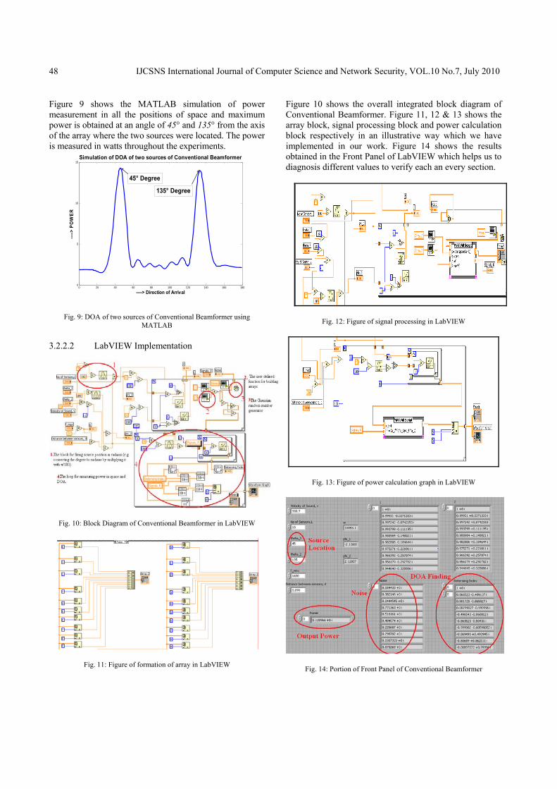
Figure 9 shows the MATLAB simulation of power measurement in all the positions of space and maximum power is obtained at an angle of 45° and 135° from the axis of the array where the two sources were located. The power is measured in watts throughout the experiments.

0 20 40 60 80 100 120 140 160 1800

5

10

15Simulation of DOA of two sources of Conventional Beamformer

----> Direction of Arrival

---->

PO

WER

45° Degree

135° Degree

Fig. 9: DOA of two sources of Conventional Beamformer using MATLAB

3.2.2.2 LabVIEW Implementation

Fig. 10: Block Diagram of Conventional Beamformer in LabVIEW

Fig. 11: Figure of formation of array in LabVIEW

Figure 10 shows the overall integrated block diagram of Conventional Beamformer. Figure 11, 12 & 13 shows the array block, signal processing block and power calculation block respectively in an illustrative way which we have implemented in our work. Figure 14 shows the results obtained in the Front Panel of LabVIEW which helps us to diagnosis different values to verify each an every section.

Fig. 12: Figure of signal processing in LabVIEW

Fig. 13: Figure of power calculation graph in LabVIEW

Fig. 14: Portion of Front Panel of Conventional Beamformer


49

Fig. 15: Result from LabVIEW of Conventional Beamformer

LabVIEW implementation of Conventional Beamformer is shown in Figure 10 which describes graphical representation of the basic mathematical equations where some of the functional blocks are shown. Figure 14 shows some portion of the front panel of LabVIEW where important blocks are shown in the figure. The output for Conventional Beamformer in LabVIEW is shown in Figure 15 and the result is same that obtained from MATLAB as shown in Figure 9.

3.2.2.3 Problem of Conventional Beamformer

The standard beamwidth for a ULA is LB /2πϕ = , and

sources whose electrical angles are closer than Bϕ will not be resolved by the Conventional Beamformer, regardless of the available data quality [6].

0 20 40 60 80 100 120 140 160 1801

2

3

4

5

6

7

8

9

10

11Simulation of DOA of two sources of Conventional Beamformer

----> Direction of Arrival

---->

PO

WER

Can not resolve outtwo sources havingdistance less thanthe beamwidth

Fig. 16: DOA of two sources of having distance less than the beamwidth in Conventional Beamformer using MATLAB

A ULA of 10=L sensors of half wavelength inter-element spacing has a beamwidth of 63.010/2 =π radians, implying that sources need to be at least 12° apart

in order to be separated by the beamformer. We have assumed the two sources located at 124.2° and 135° which is less than 12° and thus spatial aliasing takes place. Therefore, the sensors cannot resolve out two sources as desired which is shown in Figure 16.

3.2.3 Capon’s Beamformer

In an attempt to alleviate the limitation of the above beamformer, such as its resolving power of two sources spaced closer than a beamwidth, researchers have proposed numerous modifications. A well-known method was proposed by Capon which is also known as the Minimum Variance Distorsionless Response Filter. The optimization problem was posed as,

Min P(w) subject to wHa(θ) =1 … … … (21) where, P(w) is as defined in Eq. 16. This beamformer attempts to minimize the power contributed by noise and any signals coming from other directions than θ, while maintaining a fixed gain in the “look direction θ” like as a sharp spatial bandpass filter. The optimal w can be found using the technique of Lagrange multipliers, resulting in

… … … (22)

Inserting the above weight into Eq. 16 leads to the following “spatial spectrum”

… … … (23)

As it uses every available degree of freedom to concentrate the received energy along one direction, namely the bearing of interest that’s why Capon’s beamformer outperforms the classical one. The power minimization can also be interpreted as sacrificing some noise suppression capability for more focused “nulling” in the directions where there are other sources present. The spectral leakage from closely spaced sources is therefore reduced, though the resolution capability of the Capon’s beamformer is still dependent upon the array aperture and clearly on the SNR.


Here we consider two sources at 135° and 124.2° away from the axis of the array and we see that it resolves out them perfectly and its MATLAB Simulation is shown in Figure 10.


50

0 20 40 60 80 100 120 140 160 1800.1

0.15

0.2

0.25

0.3

0.35

0.4

0.45Simulation of Capons Beamformer With Two Sources having diastance less than beamwidth

----> DOA

---->

PO

WER

Resolves out twosources havingdistance less thanthe beamwidth

Fig. 17: Simulation of DOA for Capon’s Beamformer with two sources

having distance less than beamwidth


Block diagram for Capon’s Beamformer is pretty similar to that of Conventional Beamformer except in the power calculation loop as mentioned in Figure 13. It is shown in Figure 18, results from LabVIEW of Capon and the result matches with Figure 17.

3.2.4 MUSIC Algorithm

Main Features of MUSIC are [8]: • Properties of Eigen-structure of the covariance

matrix are directly Unlike others, MUSIC was indeed originally presented

as a DOA estimator. Is a frequency estimation technique. Reduces noise to a great extent.

Fig. 18: Result from LabVIEW of Capon’s Beamformer

The signal parameters which are of interest are spatial in nature and thus require the cross covariance information

among the various sensors, i.e. the spatial covariance matrix [8]

HHH tstsEttE AAxxR )}()({)}()({ ==

)}()({ ttE Hnn+ … … … (24)

P=)}()({ tstsE H… … … (25)

is the source covariance matrix and

Inn 2)}()({ σ=ttE H… … … (26)

is the noise covariance matrix. To allow for unique DOA estimates, the array is usually assumed to be unambiguous; that is, any collection of L steering vectors corresponding to distinct DOAs Kη forms a linearly independent set of

)}(),...,({ 1 Laa ηη and P has full rank [9]. In practice, an estimate R of the covariance matrix is obtained and its eigenvectors are separated into the signal and noise subspace is estimated as

HH UUIAPAR Λ=+= 2σ … … … (27)

with U unitary and Λ = diag },...,,{ 21 Lλλλ , a diagonal matrix of real eigenvalue ordered such that

0...21 >≥≥≥ Lλλλ . It is observed that any vector orthogonal to A is an eigenvector of R with the eigenvalue 2σ [9]. There are ML − linearly independent such vectors. Since, the remaining eigenvalues are all larger than 2σ , we can partition the eigenvalue/vector pairs into noise eigenvector (corresponding to eigenvalues

21 ... σλλ ==≥=+ LM ) and signal eigenvectors

(corresponding to eigenvalues 21 ... σλλ >≥≥ M ).

Hence we can write [10] Hnnn

Hsss UΛUUΛUR += … … … (28)

where IΛ 2σ=n . Since all noise eigenvectors are

orthogonal to A , the columns of sU must span the range

space of A whereas those of nU span its orthogonal complement. The projection operators onto this signal and noise subspaces are defined as [10]

HHHss AAAAUUΠ 1)( −== … … … (29)

HHHnn AAAAUUΠ 1)(1 −⊥ −== … … … (30)

MUSIC “Spatial Spectrum” is defined as

)()()()()(θθ

θθθaΠa

aa⊥= H

H

MP … … … (31)



51

This experiment assumes two sources at 124.2° and 135° which was taken in the previous experiments. The output obtained from MATLAB Simulation of MUSIC is shown in Figure 12. From the figure it is apparent that through MUSIC sensors are able to detect sources having distance less than beamwidth.

0 20 40 60 80 100 120 140 160 1800

500

1000

1500

2000

2500

3000

3500

4000

4500Simulation of MUSIC with two sources less than the beamwidth

----> DOA

----

> Sp

atia

l Spe

ctru

m

Noise is reducedto a great extent

Resolves out two sourceshaving distance less than

the beamwidth

Fig. 19: Simulation of MUSIC

We get much more improved result here since the noise is reduced to a very good extent and also it works as a very sharp spatial bandpass filter [7].


The block diagram is also similar with the Figure 6 except the power calculation loop since the difference in power calculation method. Figure 20 shows the output from LabVIEW of MUSIC algorithm and no difference exists between Figure 19 and 20.

Fig. 20: Result of MUSIC in LabVIEW

Results: From the above Three experiments it is apparent to us that MUSIC is the best algorithm for finding the DOA.

4. Performance Analysis

4.1 Performance Parameters

The performance of beamforming depends on the array type, number of multipath, number of antenna, DOA spread, number of interfernnce source and in case of hybrid antenna beamwidth. Now the similarities between beamforming and diversity techniques would be analyzed. For this, the beamforming system is redrawn in more detail as shown in figure 21.

The first similarity between beamforming and diversity technique is, in the diversity combining the diversity gain increases when the number of multipath (number of antenna) increases. Here in beamforming also the diversity gain increases with the increasing number of multipath (≠number of antenna). Another important thing is, in the system shown in Figure 21; portion after the beamformer is equivalent to the diversity circuit with two receiver antennas. In beamforming, the performance improves with both the number of antenna and also with the number of multipath. There are some other factors which have effects on the performance. They are DOA Spread and beamwidth (applicable only with Hybrid smart antenna). In diversity technique, the number of antenna is increased to increase the number of independent fading path but in beamforming, the number of antenna is increased to reduce the beamwidth and to increase the signal power.

Fig. 21: Block diagram of beamformer

One thing is to mentioned that switched beamformer and Selection Combining of diversity technique is similar in nature and Simple beamforming similar to the Maximal Ratio Combining if diversity technique. However, diversity technique is not suitable for the environment where large number of interference is present because diversity technique does not deal with the interferences. So, the diversity technique will fail in a busy environment to establish a good communication. When interference is missing, the performance of diversity and beamforming


52

should be same, if the number of antenna and the number of multipath remain the same in both cases. But simulation results show that the performance of diversity is better than the performance of beamforming even if the interference is absent. The reason is beamformer has the capability to reject the interferences but it does not have the capability to sum up all the information signals coherently which leads the receiver to make error. The following example will make the situation more transparent. Let us consider a situation as shown in Figure 22. Here two multipath signals and a smart antenna consisting of three antenna elements are considered.

In the Figure 22 signal strengths versus phase plots are shown. Two signals are distinguish by dotted line and solid line. Since number of channel transfer function is equal to the number of independent fading path, therefore two beams need to be formed for two different paths. Now if the beam 1 is formed, it would be found that in beam 1, there are components of path 2 which is not desired. Similarly, beam 2, there are components of path 1. And that is the reason that performance of beamformer is worse than the performance of diversity combining. But still the beamformer is more suitable than simple diversity combining technique since beamformer has the capability to reject interference. Again, from this example, the reason of some of the important dependencies of smart antenna system can be explained. First of all, increasing number of antenna elements distributes other multipath components over 360° of signal period and the in phase and out of phase components cancels each other. So the performance gets better. Secondly, dependency of DOA spread can also be explained with his example. If DOA spread is small, all the incoherent components of other multipath signal fall within a small range so very of them are cancelled out and performance gets poorer. On the other hand if DOA spread is large, the performance gets better. And it is expected that performance will be best when DOA spread is 360° but for linear array the performance is best at 180° since after that the beam is repeated. Now if it would be possible to reduce these incoherent signals the system performance would increase. The reason of these incoherent signals is the side lobes of the beam.

Fig. 22: Example of beamformer

4.2 Sidelobe Cancellation

There are many sidelobe cancellation techniques proposed but most of them are proposed for the receiver side. The problem of using sidelobe canceller only in the receiver side is that if the in the sidelobe canceller is used in the receiver side in the downlink conversation, the hardware complexity, cost, as well as the weight of the mobile station would be increased. But if the sidelobe canceller would be in the receiver side in the uplink conversation and in the transmitter side in the downlink conversation, the problem would not be occurred. That is the reason a sidelobe canceller for transmitter side is proposed in this paper. The problem is, there are undesired multipath components present in every signal beam. So if the signal would be transmitted in such a way so that in the receiver side the undesired signals in each beam fall in out of phase, the sidelobe would be cancelled. For this purpose a modified transmitter is designed. In which hybrid antenna elements are used to control the individual multipath components. The system is generalised for MIMO system. In MIMO system there are multiple signals transmitted simultaneously and they are decoded in the receiver side. To achieve the desired goal, every data signal is divided into number of part equal to the number of transmit hybrid antenna. Multiplied them with different weight factors then transmit them through the antennas. The system is illustrated in Figure 23.

Fig. 23: Proposed transmitter for Sidelobe Cancellation

Now only the optimum weight matrix, C should be obtained. Now the data matrix is given by,

... ... .... (32) The weight matrix to be found out is a matrix and given by

... ... ... (33)

So finally the transmitted signal matrix M becomes, ... .... ... (34)

Now the transmitted signal will be faded independently and the channel co-efficient is denoted by H matrix which is a diagonal Matrix and given by,

w1

W2


53

... ... ... (35)

There will be another phase shifting due to the antenna displacement. And the matrix is given by,

... ... ... (36)

So the received signal at the antenna elements becomes, ... ... ... (37)

Now to form the beam, the received signal matrix should be multiplied with and after beamforming each beam represents a multipath signal. So the beamformed signal matrix is given by,

... ... ... (38) It is expected,

... ... ... (39)

So if the channel transfer function and the beamforming matrix are known, the signal can be manipulated before transmission so that the incoherent signal components can be eliminated.

4.3 Hybrid Smart Antenna System

Fig. 24: Adaptive smart antenna system diagram

Figure 24 shows an N element adaptive smart antenna receiver system. Let us assume that the system is required to support M users. For a signal from any user, due to a multipath environment and the different positions of the antennas, there will be phase and amplitude differences in the signals received by the N antenna elements. The output signal from any element is a particular combination of all M signals and their multipath signals. These signals will first go through RF to IF blocks, and then they will be converted to a digital

stream by analog-to-digital converters and sent to the data bus. There are M beamforming blocks connected to the data bus. Each of these blocks needs to process N digital streams obtained from the data bus, and generate a pattern to receive the signal from one of the M users.

Fig. 25: Adaptive pattern of one beamforming block

Fig. 25 shows a pattern formed by a beam-forming block shown in Figure 1. Multipath signals and undesired interferences are noted by solid-arrow lines and dash-arrow lines, respectively. As may be seen, an adaptive implementation can dynamically point pattern peaks to desired and multipath signals, and adjust the nulls to cancel unwanted interferences. With the increase in the number of total antenna elements, the system complexity increases significantly. Figure 26 shows a switched-beam smart antenna system formed by N directional antenna elements. Each antenna covers an angle range of 360° / N. As shown in Figure 27, the system can automatically switch to an antenna that has its main beam in the domain of the desired signal. Because the preformed pattern has a narrow main beam, most multipath and interference signals will fall into the side lobe range, resulting in suppression of these signals and improved system performance. Comparing this with the adaptive implementation, it may be noted from Figure 27 that the switched-beam method cannot make full use of the multipath signals, and cannot be used to cancel interferences when located in the main lobe. Thus, the performance of a switched-beam system is less optimal when compared with an adaptive system. This will also be confirmed in Section IV by simulation of several representative cases. Figure 28 shows a proposed alternative hybrid smart antenna system. The proposed system described in this paper combines the advantages of both switched-beam and adaptive systems. Unlike traditional adaptive antenna arrays, the proposed system uses directional elements to achieve additional antenna gain. It does have beamforming capabilities to cancel interferences but uses a smaller number of signals than traditional adaptive systems. Through the proper design of the proposed system, it may be expected that it is possible to achieve a performance similar to that of an


54

adaptive system with the advantage of using a lesser number of signals in the adaptive process. Similar to the traditional switched beam array process, signal selection will be based on combining the strongest signals in the overall array.

Fig. 26: Switched beam smart antenna system diagram

Fig. 27: Pattern of switched beam smart antenna

Fig. 28: Proposed smart antenna system

As shown in Figure 28, the proposed system inherits part of the characteristics of the switched-beam system, in that it adopts directional antenna elements. It will be described in Section IV that different coverage angles should be chosen in different multipath scenarios to obtain the best performance.

The arrangement in Figure 28 also borrows some digital beamforming technology used in adaptive systems, but in this case the beam-forming will be done more efficiently using a reduced number of signals. There are additional blocks (N to NS selector) that select only the NS (NS < N) strongest signal streams from total N streams on the data bus. Considering the slow angle movement of mobile users and the relatively wide beamwidth of the radiation pattern of antenna elements, the N to NS switches do not need to be updated in real time. It will be shown that in most cases when using the arrangement in Figure 28, performance similar to that of an eight-element adaptive system can be achieved by using a value of NS as small as 2. It will also be shown that as NS increases, the performance will continue to improve; but the system complexities will also increase and ultimately converge to a fully adaptive antenna array.

4.4 Assumptions and Description of System Model

Fig. 29: Block diagram of an N-element beam forming smart antenna system

Figure 29 shows a block diagram of an N-element beam forming smart antenna system. The baseband signal x ( t ) received by the antenna array is given by

… … … (40) where Ud and Ui are matrices of the channel transfer functions of the multipath signal and interferences, respectively. sd and si

are vectors of the multipath signals and interferences, respectively, n is the system noise. The channel transfer functions and the signal vectors are given by

… … … (41)

… … … (42)

… … … (43)


55

… … … (44)

… … … (45)

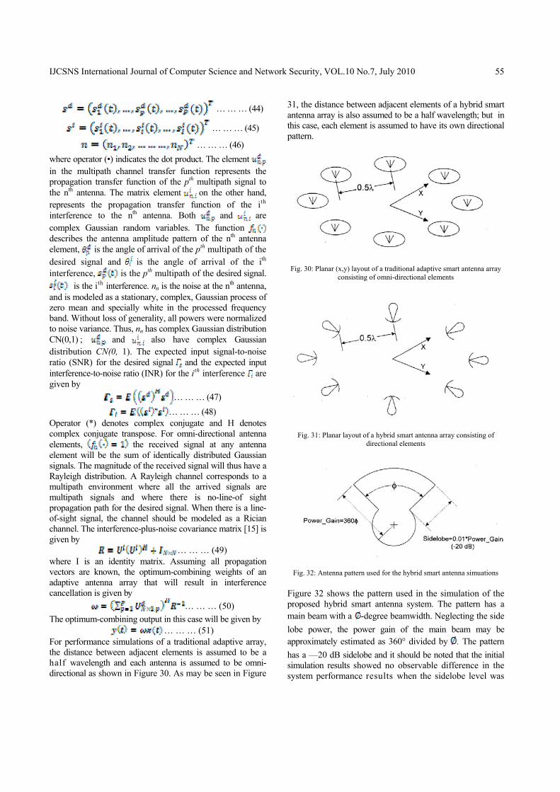
… … … (46) where operator (•) indicates the dot product. The element in the multipath channel transfer function represents the propagation transfer function of the pth multipath signal to the nth antenna. The matrix element on the other hand, represents the propagation transfer function of the ith interference to the nth antenna. Both and are complex Gaussian random variables. The function describes the antenna amplitude pattern of the nth antenna element, is the angle of arrival of the pth multipath of the desired signal and is the angle of arrival of the ith

interference, is the pth multipath of the desired signal. is the ith interference. nn is the noise at the nth antenna,

and is modeled as a stationary, complex, Gaussian process of zero mean and specially white in the processed frequency band. Without loss of generality, all powers were normalized to noise variance. Thus, nn has complex Gaussian distribution CN(0,1) ; and also have complex Gaussian distribution CN(0, 1). The expected input signal-to-noise ratio (SNR) for the desired signal and the expected input interference-to-noise ratio (INR) for the ith interference are given by

… … … (47) … … … (48)

Operator (*) denotes complex conjugate and H denotes complex conjugate transpose. For omni-directional antenna elements, the received signal at any antenna element will be the sum of identically distributed Gaussian signals. The magnitude of the received signal will thus have a Rayleigh distribution. A Rayleigh channel corresponds to a multipath environment where all the arrived signals are multipath signals and where there is no-line-of sight propagation path for the desired signal. When there is a line-of-sight signal, the channel should be modeled as a Rician channel. The interference-plus-noise covariance matrix [15] is given by

… … … (49) where I is an identity matrix. Assuming all propagation vectors are known, the optimum-combining weights of an adaptive antenna array that will result in interference cancellation is given by

… … … (50) The optimum-combining output in this case will be given by

… … … (51) For performance simulations of a traditional adaptive array, the distance between adjacent elements is assumed to be a half wavelength and each antenna is assumed to be omni-directional as shown in Figure 30. As may be seen in Figure

31, the distance between adjacent elements of a hybrid smart antenna array is also assumed to be a half wavelength; but in this case, each element is assumed to have its own directional pattern.

Fig. 30: Planar (x,y) layout of a traditional adaptive smart antenna array consisting of omni-directional elements

Fig. 31: Planar layout of a hybrid smart antenna array consisting of directional elements

Fig. 32: Antenna pattern used for the hybrid smart antenna simuations

Figure 32 shows the pattern used in the simulation of the proposed hybrid smart antenna system. The pattern has a main beam with a -degree beamwidth. Neglecting the side lobe power, the power gain of the main beam may be approximately estimated as 360° divided by . The pattern has a —20 dB sidelobe and it should be noted that the initial simulation results showed no observable difference in the system performance results when the sidelobe level was


56

varied by as much as ±10 dB from the utilized —20 dB value. For the case of an eight-element array with equal to 45°, the main beam of all the elements will be placed side-by-side to provide the 360° coverage. If is less than 45° there will be gaps that cannot be covered by the collective main beams of the eight-element array, and if is larger than 45° there will be an overlap between the patterns from the various antenna elements. One thing that needs to be mentioned is that (•) in (……..) and (……………) is the amplitude pattern instead of the power pattern, hence a square root operator is needed to get (•) from the power pattern normally measured in antenna characterization. Two kinds of communication systems, TDMA and CDMA, were simulated in this paper. For a TDMA system, smart antennas are only used to overcome multipath fading and no co-channel interference is assumed. For a CDMA system, all users share the same frequency and channels are distinguished by different codes. Each user thus interferes with other users who are occupying the same frequency band. In a CDMA system; therefore, a smart antenna is used to overcome both multipath fading and interference. Binary phase shift keying (BPSK) modulation is used in all simulations; therefore, the output of an optimum combining in (……..) can be simplified to Re(y(t)). Also, 500000 random cases were simulated for each SNR value and for each operating case of the proposed antenna structure.

-20 -10 0 10 20 30 4010-4

10-3

10-2

10-1

100

SNR in dB

Erro

r pro

babi

lity

Performance graph

Fadingsidelobe cancellor BPSKsidelobe cancellor 4-QAMsidelobe cancellor 16-QAMsidelobe cancellor 64-QAM

FadingEffect

BPSK

64-QAM16-QAM

4-QAM

Fig. 33: BER and fading effect on the system for different modulation schemes

5. Conclusion

In this paper, the theory of Array Signal Processing is introduced for voice signals to find the location of source. It can be inferred that estimates of an arbitrary location of signal source can be performed with moderate accuracy if the data collection time is sufficiently long or the SNR is

adequately high, and the signal model is sufficiently accurate. A hardware implementations using LabVIEW data acquisition card that would use the blocks developed in LabVIEW in real-time is in progress. We have tried our level best to make this work a successful one. In concluding, the recent advances of the field, we think it is safe to say that the spatial based subspace methods and in particular, the more advanced parametric methods have clear performance improvements to offer as compared to beamforming methods. Resolution of closely spaced sources (within fraction of a beamwidth) have been demonstrated and documented in several experimental studies. However, high performance is not for free. The requirements on sensor and receiver calibration, mutual coupling, face stability, dynamic ranges etc. become increasingly more rigorous with higher performance specifications. Thus in some applications the cost for achieving within-beamwidth resolution may still be prohibitive. References [1] Monson H. Hayes, Statistical Digital Signal Processing and

Modeling, John Wiley and Sons, INC., 1996. [2] Henry Stark, John W. Woods, Probability and Random

Processes with Application to Signal Processing, Pearson Education, 2002.

[3] Hamid Krim and Mats Viberg, “Two Decades of Array Signal Processing”, IEEE Signal Processing Magazine, pp. 67-90, July, 1996.

[4] Claiborne McPheeters, James Finnigan, Jeremy Bass and Edward Rodriguez,”Array Signal Processing: An Introduction” Version 1.6: Sep 12, 2005.

[5] A.Leshem and A.J.van der Veen, “Direction-of-Arrival estimation for constant modulus signals,” IEEE Trans. Signal Processing; vol. 47, pp.3125-3129, Nov 1999.

[6] Alan V. Oppenheim, Alan S. Willsky and S. Hamid Nawab, Signals and Systems, Pearson Education, 2004.

[7] Robert F. Coughlin and Frederick F. Driscoll, Operational Amplifiers and Linear Integrated Circuits, Prentice-Hall of India Private Limited, 2006.

[8] John G. Proakis and Dimitris G. Manolakis, Digital Signal Processing Principles, Algorithms and Applications, Prentice-Hall of India Private Limited, 2006.

[9] Frank Ayres, JR, Theory and Problems of Matrices, McGraw-Hill Book Company, New York, 1974.

[10] J.J.Shynk and R.P.Gooch, “The constant modulus array for co-channel signal copy and direction finding, ”IEEE Trans. Signal Processing; vol. 44, pp.652-660, Mar.1996.

[11] S. Bellofiore et al., “Smart Antenna System Analysis, Integration and Performance for mobile Ad-Hoc networks (MANET’s),” IEEE Trans. Antennas Propagat., vol. 50, pp. 571-581, May 2002.

[12] M. Ho, G. Stuber, and M. Austin, “Performance of Switched-beam smart antennas for cellular radio system”, IEEE Trans. Vehic. Technol., Vol. 47, pp. 10-19, Feb. 1998.

[13] R. C. Bernhardt, “The use of multiple-beam directional antennas in wireless messaging system”, In Proc. IEEE Vehicular Technology conf., 1995, pp. 858-861.


57

[14] A. F. Naguib, A. Poulraj, and T. Kailath, “Capacity Improvement with BS Antenna arrays in cellular CDMA”, IEEE Trans. Vehic. Technol., Vol. 43, pp. 691-698, Aug. 1994.

[15] P. Strobach, “Total least Squares phased averaging and 3-D ESPRIT for joint azimuth-elevation-carrier estimation”, IEEE Trans. Signal Processing, Vol. 49, pp. 54-62, Jan 2001.

[16] B. Widrow and S. D. Stearns, Adaptive signal processing. Englewood cliffs, NJ: Prentice-Hall 1985.

Md. Shahedul Amin received his B.Sc. degrees in Electrical and Electronic Engineering from Islamic University of Technology (IUT) in 2008. His research interest lies in Signal Processing, Biomedical Engineering and Communication Engineering. Currently he is doing his M.Sc. at IUT in

Biomedical Signal Processing.

Md. Riyasat Azim received his B.Sc. degrees in Electrical and Electronic Engineering from Islamic University of Technology (IUT) in 2008. His research interest lies in Signal Processing, Biomedical Engineering and Communication Engineering. Currently he is

doing his M.Sc. at IUT in Signal Processing.

Syed Prantik Rahman received the B.Sc. degree in Electrical and Electronic Engineering from Islamic University of Technology, Bangladesh in 2008. He is now receiving his Masters of Engineering Degree in Wireless Engineering from University of Sydney, Australia. During 2007-2008, he

completed his thesis in Genomic Signal Processing. Now he is doing his Masters Program Thesis in Mobile Networks in Practical Environment.

Md Ferdous Habib received his B.Sc. degree in Electrical and Electronic Engineering from Islamic University of Technology (IUT) in 2008 majored in telecommunications. He also completed Master in Engineering (M.E) from University of Sydney in July 2010 majored in Wireless Engineering. He has

studied a detail about mobile communication, satellite communication, antennas and other related regions. Now he stays in Sydney to complete his Master in Engineering Management (M.E.M) from University of Technology Sydney (UTS).

Md. Ashraful Hoque received his B.Sc. degrees in Electrical and Electronic Engineering from Bangladesh University of Engineering and Technology (BUET) in 1986. He has completed his M.Sc. in 1993 and Ph.D. in 1996 from Memorial University of Newfoundland (MUN) in the field of

Automatic Control of Intelligent Motor Drive. His research interest lies in Signal Processing, Biomedical Engineering and Power Electronics. Currently he is working as a Professor in IUT.

estimation of direction of arrival (doa) using real- time...

Documents