estimation of continuous time processes via the empirical
TRANSCRIPT

Estimation of Continuous Time Processes Via the
Empirical Characteristic Function
George J. Jiang� and John L. Knight|
This Version: August 2000
�George J. Jiang, Department of Finance, Schulich School of Business, York University, 4700 Keele Street,
Toronto, Ontario, Canada M3J 1P3. Tel: (416) 736-2100 ext. 33302, (416) 736-5073 and Fax: (416) 736-5687.
E-mail: [email protected].�John L. Knight, Department of Economics, University of Western Ontario, London, Ontario, Canada,
email: [email protected].

Estimation of Continuous Time Processes Via the Empirical
Characteristic Function
Abstract
This paper examines a particular class of continuous-time stochastic processes commonly
known as af¿ne diffusions (AD) and af¿ne jump-diffusions (AJD) in which the drift, the
diffusion and the jump coef¿cients are all af¿ne functions of the state variables. By deriv-
ing the joint characteristic function associated with a vector of observed state variables for
such models, we are able to examine the statistical properties of these diffusions and jump-
diffusions as well as develop an ef¿cient estimation technique based on empirical character-
istic functions (ECF) and a GMM estimation procedure based on exact moment conditions.
The estimators developed in this paper are in stark contrast to those available in the literature
in the sense that our methods require neither discretization nor simulation. We demonstrate
that our methods are in particular useful for the AD and AJD models with latent variables, i.e.
the case where some of the state variables are unobserved. We illustrate our approach with
a detailed examination of the continuous-time square-root stochastic volatility (SV) model,
along with an empirical application using S&P 500 index returns.
JEL Classi¿cation: C13, C22, C52, G10
Key Words: Af¿ne Diffusion, Af¿ne Jump-Diffusion, Empirical Characteristic Function
(ECF), Generalized Method of Moments (GMM), Stochastic Volatility (SV)

1 Introduction
The estimation of continuous-time stochastic processes, especially those with unobserved or
latent variables, has posed a challenge to statisticians and econometricians for some time.
In ¿nancial applications, due to the unavailability of a continuous sample of observations,
estimation has usually been performed by ¿rst discretizing the model and then applying var-
ious moment based estimation methods, e.g. the generalized method of moment (GMM)
approach in Chan, Karolyi, Longstaff, and Sanders (1992). In the econometrics and statisti-
cal literature, new estimation techniques are mostly developed based on simulation methods,
e.g. the simulated method of moments (SMM) in Duf¿e and Singleton (1993), and the ef¿-
cient method of moments (EMM) in Gallant and Tauchen (1996). The application of these
approaches has had varying success due mainly to the need of both discretizing the model
and simulating sample paths. Beside the intensive computation involved, these two steps can
compound the estimation errors and consequently may lead to poor ¿nite sample properties.
While there are a few speci¿c models for which the maximum likelihood (ML) estimation
is possible as there exist explicit closed form transition density functions, these models have
not proved to be popular in ¿nance due to unrealistically simplistic model speci¿cations. In
the multivariate framework, the estimation problem becomes even more dif¿cult and partic-
ularly so if some of the state variables are unobserved.
However, it has recently be noticed that there is a class of continuous-time stochastic
processes where, while the transition density functions are not known, their Fourier transfor-
mation, i.e. the characteristic functions are known. These processes are the so-called af¿ne
diffusions (AD) and af¿ne jump-diffusions (AJD) developed and popularized in a series of
papers by Duf¿e and Kan (1996), Dai and Singleton (1999), and Duf¿e, Pan and Singleton
(1999). Since these processes are Markovian with, in many cases, explicit closed form con-
ditional characteristic functions, it opens the door for alternative estimation techniques. Two
1

recent papers which have exploited the idea of developing new estimation methods based on
conditional characteristic functions are Chacko and Viceira (1999) and Singleton (1999).
This paper also examines the AD and AJD models via their associated characteristic
functions. However, in our case we use the unconditional joint characteristic function rather
than the conditional characteristic function. Based on the unconditional joint characteristic
function, we examine the statistical properties of these models and develop new estimation
strategies. In particular, our interest centers on models where some of the state variables are
unobserved. The estimation of these models, which include the popular stochastic volatility
model as a special case, poses even more of a challenge to statisticians and econometricians.
Singleton (1999) proposes the use of the conditional characteristic function along with sim-
ulation and develops a SMM estimator. Our approach exploits the explicit functional form
of the unconditional joint characteristic function to develop an ef¿cient estimation procedure
based on the empirical joint characteristic function. Since there is an exact one-to-one cor-
respondence between the characteristic function and the distribution function, the empirical
characteristic function (ECF) contains the same amount of information as the empirical dis-
tribution function (EDF). Consequently, the ECF method has the same asymptotic ef¿ciency
as the maximum likelihood (ML) method. Moreover, since the exact moment conditions
of the stochastic processes are readily available from the analytical characteristic functions,
an alternative approach is also proposed in this paper for the AD and AJD models via the
generalized method of moments (GMM). The estimators developed in this paper are in stark
contrast to those available in the literature in the sense that our methods require neither dis-
cretization nor simulation. More importantly, our methods are particularly useful for the
AD and AJD models with latent variables, i.e. the case where some of the state variables
are unobserved. We illustrate the approach of analyzing the statistical properties of AD and
AJD models based on the joint characteristic function with two examples, the square-root
process in the univariate case and the SV model in the bivariate case. An application of the
2

estimation methods is undertaken for the SV model using the S&P 500 index returns
Section 2 examines the general AD and AJD models and the joint characteristic function
in both the situation where all the state variables are observed and that where only some of
the state variables are observed. We show how from the joint characteristic function we can
examine the statistical properties of these processes. In section 3 we consider the estima-
tion problem and develop, in particular, two estimators, the empirical characteristic function
(ECF) approach and the GMM approach for the AD and AJD models with unobserved or la-
tent variables. Section 4 involves an empirical application of our techniques to the SV model
using daily S&P 500 index returns, along with further discussion on the issues related to the
implementation of the ECF method. A brief conclusion is contained in Section 5.
2 The Continuous Time Stochastic Processes
We consider a general continuous time af¿ne jump-diffusion (AJD) model, with af¿ne diffu-
sion (AD) model as a special case, as de¿ned in Duf¿e, Pan and Singleton (1999). Using the
same notation as in Duf¿e, Pan and Singleton (1999), we ¿x a probability space ElcI c � �
and an information ¿ltration EI � � ' iI � G | � fj, and suppose that f � is a Markov process
in some state space G 5 U � , following the stochastic differential equation (SDE):
_f � ' >Ef � �_|n jEf � �_` � n _~ � (1)
where ` � is an EI � �-standard Brownian motion in U�, >E�� G G $ U
�and jE�� G G $ U
�
are respectively the drift function and diffusion function, and ~ is a pure jump process whose
jumps have a ¿xed probability distribution M on U�
and arrive with intensity ibEf � � G | �
fj, for some bE�� G G $ dfc4�. The initial value of the stochastic process f � is assumed to
follow a trivial distribution. For f � to be a well-de¿ned Markov process, regularity condi-
tions on the ¿ltration EI � � ' iI � G | � fj and restrictions on the state space as well as on the
coef¿cient functions of the stochastic process, namely EGc >E��c jE��c bE��cM �, are required.
3

For technical details, see e.g. Ethier and Kurtz (1986), Duf¿e, Pan and Singleton (1999), Dai
and Singleton (1999), and Duf¿e and Kan (1996).
The continuous time jump-diffusion (JD) process de¿ned in (1) is often used in the ¿-
nance literature to model the dynamics of asset return, index return, exchange rate, and in-
terest rate, etc. Intuitively, the drift term >E�� represents an instantaneous deterministic time
trend of the process, the diffusion term jE��jE�� � represents an instantaneous volatility of the
process when no jump occurs, and the jump term ~ � captures the discontinuous change of the
sampling path with both random arrival of jumps and random jump sizes. More speci¿cally,
as noted in Duf¿e, Pan and Singleton (1999), conditional on the path of f � , the jump times of
~ � are the jump times of a Poisson process with time varying intensity ibEf � � G f � r |j,
and the size of the jump of ~ � at a jump time � is independent of if � G f � r �j and
follows the probability distribution M .
For convenience and tractability, many ¿nancial models impose an “af¿ne” structure on
the coef¿cient functions >E��c jE��jE�� � c and bE��, i.e. all of these functions are assumed to
be af¿ne on G. Using the notation in Duf¿e, Pan and Singleton (1999), we have
>Ef � � ' g � ng � f � c
djEf � �jEf � ��o � ' dM � o � n dM � o � f � c
bEf � � ' , � n , � f �
where g ' Eg � c g � � 5 U� � U
����c M ' EM � cM � � 5 U
���� � -���� ��
c , ' E, � c , � � 5
U�U � . Let }ES� 'U
U � i TiS �5j_M E5� be the jump transform whenever the integral is well
de¿ned, where S 5 F � the set of n-tuples of complex numbers, }E�� determines the jump size
distribution. It is obvious that the set of “coef¿cients” or parameters EgcMc ,c }� completely
speci¿es the AJD process and determines its statistical properties, given the initial condition
f � . When the jump intensity is set as zero, i.e. bE�� ' f, the process is referred to as the
af¿ne diffusion (AD) process.
Dynamic properties of the jump-diffusion (JD) process de¿ned in (1) are determined
4

by the transition density functions which, under regularity conditions, satisfy both the Kol-
mogorov forward and backward (or Fokker-Planck) equations of the Markov process. How-
ever, the transition density functions of the diffusion and jump-diffusion process in general
do not have a closed analytical form. For instance, in the simplest univariate pure-diffusion
case, i.e. ? ' �c bE�� ' f, the Ornstein-Ulenbeck process and the square-root diffusion
process are the only two well-known processes with explicit transition density functions.
For these two processes, both the drift function >E�� and the diffusion function j�E�� are of
linear structure. The functional forms of the transition densities corresponding to speci¿ca-
tions essentially different from the above two processes are not known explicitly, see Wong
(1964).
As we mentioned in the introduction, since there is an exact one-to-one correspondence
between the characteristic function and the distribution function, an alternative expression
of the statistical properties of the model is given by the characteristic function of the state
variables. Duf¿e, Pan and Singleton (1999) showed that under the “af¿ne” structure, the
conditional characteristic function of the jump-diffusion process as de¿ned in (1) has a closed
form. Using their results, we have the characteristic function off ����� conditional onf � given
by
�E�(f ����� mf � � ' .di Ti��f ����� jmf � o
' i Ti�E� c �� n(E� c ���f � j (2)
where (E�� and �E�� satisfy the following complex-valued Ricatti equations:
Y(E� c ��
Y�' g
�� (E� c �� n
�
2(E� c ��
�M � (E� c �� n , � E}E(E� c ���� �� (3)
Y�E� c ��
Y�' g
�� (E� c �� n
�
2(E� c ��
�M � (E� c �� n , � E}E(E� c ���� �� (4)
with boundary conditions: (Efc �� ' ��c �Efc �� ' f. With certain speci¿cation of the
coef¿cient function EgcMc ,c }�, explicit solutions of (E�� and �E�� can be found. In other
5
cases, as noted in Duf¿e, Pan and Singleton (1999), the solution would have to be found
numerically. With explicit solutions of (E�� and �E��, it appears that it would be easier to
investigate the statistical properties of the model in the frequency domain than in the time
domain.
In practice, in order to investigate the joint sampling properties of the jump-diffusion
process on the one hand and eliminate the “start-up” effect of the initial condition on the
other, the unconditional joint probability distribution or the unconditional joint character-
istic function of the state variables if ��� c f ��� c ���c f ��� j over time i| � c | � c ���c |� j rather than
the conditional probability density function or conditional characteristic function are often
required. In the next section, we will see that these joint distribution functions or joint char-
acteristic functions will be needed for the estimation of the stochastic processes. Due to the
Markov property, the joint probability distribution is given by the conditional probability dis-
tribution and the marginal distribution of the initial condition, namely sEf ��� c f ��� c ���c f � � � '
sEf � � �T�������� � sEf ��!#" � mf ��! �. Obviously the joint density function cannot have closed form if
the transition density function is not explicitly known. Again, our hope is to resort to the
unconditional joint characteristic function. Even though the characteristic function does not
share the nice iterative property as the distribution function, the following lemma shows that
in an af¿ne jump-diffusion framework, when the marginal characteristic function of the ini-
tial condition is available, we still can have a closed form for the joint characteristic function.
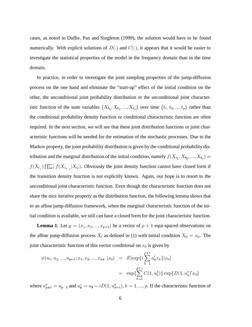
Lemma 1: Let + ' E% � c % � c ���c %�$� � � be a vector of R n � equi-spaced observations on
the af¿ne jump-diffusion process f � as de¿ned in (1) with initial condition f � ' % � . The
joint characteristic function of this vector conditional on % � is given by
�E� � c � � c ���c ��%� � (% � c % � c ���c %�%� � m% � � ' .di Ti��%� �[
& �'��� & % & jm% � o
' i Ti�$� �[
& � ��E�c �
(& �j i Ti(E�c �(� ��% � j
where �(�$�'� ' ��%� � and �
(& ' � & � �(E�c �(& � � �c & ' �c ���c R. If the characteristic function of
6

% � is available, i.e.
.de)�* +$,
o ' �E�(% � �
then, the unconditional characteristic function of + is given by
�E� � c � � c ���c ��$�'� ( % � c % � c ���c %�$� � � ' i Ti�$� �[
& � ��E�c �
(& �j�E(E�c �(� �( % � � (5)
Proof : See Appendix.
Remark 1: In the case thatf � is stationary, the marginal density function and the marginal
characteristic function of the process can be derived from the conditional density function
and the conditional characteristic function respectively, namely sEf � ' % � � ' *�4 �$-.��/
sEf � ' % � mf ��� � ' % �0� � � and �E�(f � � ' *�4 �$-.��/ �E�(f � mf ���1� ' % ��� � �. Statistical
properties, both static and dynamic, can be derived from the characteristic functions as both
the cumulants and moments can be calculated easily when the characteristic function has a
closed analytical form.
As an application of the above lemma and an illustration of how the characteristic func-
tion can be used to study the statistical properties of the stochastic process, we now examine
the following example.
Example 1: The Square-Root Diffusion Process. Consider the following univariate pure
diffusion process
_T � ' qEk� T � �_|n jT�32 �� _` � (6)
with af¿ne structure on both the drift function >ET � � ' qEk � T � � and diffusion function
j�ET � � ' j
�T � . This process is known to be a positive process with a reÀecting barrier at
zero, which is attainable when 2qk j�, and has been used in Cox, Ingersoll and Ross
(1985) to model the nominal interest rates and Bailey and Stulz (1989) and Heston (1993) to
model the conditional volatility of asset returns. Solving from (3) and (4) for (E�� and �E��,
7

we have the conditional characteristic function
�E�(T � ' � � mT � ' � � � ' i TE�E�c �� n(E�c ��� � �
' i Ti�2qk
j� *?E�� ��
S� n
��e�145�
�� ��*S� � j (7)
where S ' 2q*Ej�E� � e
�145���. Via Fourier inversion of the conditional characteristic func-
tion, the transition density function can be obtained as sET � ' � � mT � ' � � � ' Se� ) ��6
E6) � 7 2
�
U 7 E2E�D��32 �
� with T � taking nonnegative values, where � ' S� � e �145� , D ' S� � , ^ '� 498: � � �c
and U 7 E�� is the modi¿ed Bessel function of the ¿rst kind of order ^. The transition den-
sity function is non-central chi-square, ��d2S� � ( 2^ n 2c 2�o, with 2^ n 2 degrees of free-
dom and parameter of noncentrality 2� proportional to the current level of the stochastic
process. The conditional expected value and variance of T � is given by .dT � mT � ' � � o '
� � e �145� nkE��e�145�
�c T @odT � mT � ' � � o ' ;, : �4 Ee
�145� �e� � 45�
�n8 : �� 4 E��e
�145���� If the process
displays the property of mean reversion Eq : f�, the process is stationary and its marginal
distribution can be derived from the transition density, which is a gamma probability density
function, i.e., sET � ' � � � ' <=
>@? �BA �� ���� e
� <C;ED where / ' 2q*j�
and r ' 2kq*j�, with mean k
and variance kj�*2q. Similarly the marginal characteristic function can be derived from the
conditional characteristic function as �E�(T � � ' E�� � )�: �� 4 �� � 498C2 : � .
With the direct application of Lemma 1, the joint characteristic function of i� � c � � c ���c ��$� � j
as a vector observations of T � with initial condition T � ' � � is given by
�E� � c � � c ���c ��$� � ( � � c � � c ���c ��%� � � ' .d.di Ti��%� �[
& � �� & � & jom� � o
' i Ti�%� �[
& � ��E�c �
(& �j.di Ti(E�c �(� �� � jo
where �(�%� � ' ��$� c �
(& ' � & � �(E�c �(& �'� � for & ' �c 2c ���c R with (E�� and �E�� given by the
solutions in (7) for this particular example. Now since � � has a gamma marginal (stationary)
distribution, we have
�E� � c � � c ���c ��$� � ( � � c � � c ���c ��%� � � ' i Ti�$� �[
& � ��E�c �
(& �jE�� (E�c �(� �j
�
2q�� � 498C2 : �
8

A widely used and also very important class of stochastic processes in ¿nance literature
is the one that involves the unobservable or latent state variables, e.g. the stochastic volatility
(SV) model. As we will see in the next section, the estimation of such a class of models has
posed a great challenge to econometricians. We partition the whole vector of f � into two
sub-vectors, i.e. f � ' E7�� c T
�� ��c where 7 � 5 U F c ? : 6 : fc is the vector of observed
state variables and T � 5 U � � F is the vector of unobserved or latent state variables. Instead
of ¿nding the joint sampling properties of the whole vector of state variables f � , now we are
interested in only the sub-vector of f � , namely 7 � . While we know that the vector process
f � is Markovian, 7 � , as a sub-vector of f � , is not necessarily Markovian. That is, the future
values of 7 � may be dependent upon not only its current observation, but also its historical
observations, and in certain cases even its entire history. In the non-Markov case, the joint
probability function sEr � , c r �G� c ���c r ��� � does not have the nice iterative property any more.
Again, when its analytical functional form is not available, we hope to resort to the joint
characteristic function. Specializing earlier results, we have
�E��c �2( r ����� c � ����� mr � c � � � ' .di Ti����r ����� n ��2
�� ����� jmr � c � � o
' i Ti�E� c ��c �2� n(�E� c ��c �2��r � n(2E� c ��c �2�
�� � j (8)
where�E� c ��c �2� ' �E� c ��c E(�E� c ��c �2��c (2E� c ��c �2�
�� ' (E� c ��
�with � ' E��
�c �2
���.
Further, we note
�E�( r ����� mr � c � � � ' .di Ti���r ����� jmr � c � � o
' i Ti�E� c �c f� n(�E� c �c f��r � n(2E� c �c f�
�� � j
Therefore we have the following lemma.
Lemma 2: Letf � be the af¿ne jump-diffusion process de¿ned in (1) withf � ' E7�� c T
�� ��,
and + ' Er � c r � c ���c r�%� � � be a vector of Rn� equi-spaced observations on the partial stochas-
tic process 7 � with initial condition f � ' % � . The joint characteristic function of the vector
9

+ conditional on % � is given by
�E�� � c �� � c ���c ���$� � ( r � c r � c ���c r�%� � m% � � ' .di Ti��%� �[
& � ���� & r & jm% � o
' i Ti�%� �[
& �'��E�c ��
(& c �2(& �j i Ti(E�c ��
(� c �2
(� ��% � j
where ��(�$� � ' ���$� � c �2
(�$�'� ' f, ��
(& ' �� & � �(�E�c ��(& � � c �2
(& � � �, and �2(& ' ��(2E�c
��(& � � c �2
(& � � � for & ' �c 2c ���c R. If the characteristic function of % � is available, i.e.
.de)�* +$,
o ' �E�(% � �
Then, the unconditional joint characteristic function of + is given by
�E�� � c �� � c ���c ���%� � ( r � c r � c ���c r�%� � �
' i Ti�$� �[
& � ��E�c ��
(& c �2(& �j�E(E�c ��
(� c �2
(� �(% � � (9)
Proof : See Appendix.
Remark 2: As noted in Remark 1, for stationary processes the marginal density function
can be derived from the transition density, and the marginal characteristic function can be
derived from the conditional characteristic function. In the asset return models, it is quite
often the case that not the whole vector of f � is stationary. Instead, only part of the process
is stationary, and the rest of the process is ¿rst difference stationary. For instance, in the
following stochastic volatility asset return model, while the stochastic volatility is speci¿ed
to be stationary, the logarithmic asset prices are modeled as ¿rst difference stationary, in
other words, the asset returns are stationary. Without loss of generality, we assume that T � is
stationary and {7 � ' 7 � �7 ����H is stationary, that is E{7 � c T � � is a stationary process. Instead
of analyzing the joint characteristic function of ir � c r � c ���c r�%� � j, we can derive the joint
characteristic function of i{r � c{r � c ���c{r�%� � j, in which only the marginal characteristic
function of � � is needed. For 7 � to be ¿rst difference stationary, certain restrictions on the
parameter set EgcMc ,c }� are required. One set of suf¿cient conditions is that the elements of
10

g � c M � c , � and } corresponding to the 7 � equations are all zero, i.e. the state variables 7 � do
not appear directly in its own dynamic process. Thus the solution to the SDE (3) for (E� c ��,
corresponding to state variables 7 � , is (E� c �� ' (Efc �� ' ��. We illustrate Lemma 2 in
general and this special case in particular with the following example.
Example 2: The Square-Root Stochastic Volatility Model. Consider the following asset
return process with stochastic conditional volatility for the logarithmic asset prices r � 1
_r � ' >_|n T�32 �� _` �
_T � ' qEk� T � �_|n jT�32 �� _` ;�
_` � _` ;� ' 4_|c | 5 dfc A o (10)
This continuous-time SV model has been widely used in the ¿nance literature for asset return
dynamics as it allows for a closed-form solution for European option prices. As in Singleton
(1999), the drift term of the asset return process is speci¿ed as a constant. It is noted that
when the drift term of the asset return process is speci¿ed as a linear function of the state
variable T � , both the European option prices and the conditional characteristic function of
the asset return will still yield closed forms. The speci¿cation of the instantaneous volatility
process in the above model guarantees the nonnegativeness of the volatility. The solution of
the square-root process in (6) or (10) can be written as
T ��� � ' E�� e�14�k n e
�14T � n
] ��� �� je
�14 ? ��� �I� � AT�32 �� _` ;�
which is of an �-E�� form, where " ��� � 'U ���'�� je
�14 ? ���'�E� � AT�32 �� _` ;� is a martingale. Thus
the process can be viewed as an �-E�� process with heteroskedasticity. The parameter q
measures the intertemporal persistence of the volatility process, and the correlation between
_` ;� and _` � measures the level of asymmetry of the conditional volatility. In particular,
when 4 f we have the so-called “leverage effect”.
1Please note that in this example, v J denotes the random process.
11

Statistical properties of the stochastic volatility process have been discussed in detail in
Example 1. Due to the lack of explicit solutions to the continuous-time asset return process
with stochastic volatility as de¿ned in (10), there has been no formal derivation or discussion
of the statistical properties of the asset return process. However, from a straightforward ap-
plication of Lemma 2 to the process E{r � c T � �, we can derive the unconditional characteristic
function of the asset return {r � ' r � � r ���K� , as well as the joint characteristic function of the
asset returns. Lemma 3 presents the joint characteristic function of asset returns, followed
by the discussion of both static and dynamic properties.
Lemma 3: Let r � be the stochastic process de¿ned in (10), given r � and that T � ' � �
follows its marginal distribution, the joint characteristic function of {r � ' r � � r � c{r � '
r � � r � c ���c and {r�%� � ' r�%� � � r� c where R � �c i.e.,
�E� � c � � c ���c ��%� � ( {r � c{r � c ���c{r�$�'� � ' .di Ti��$� �[
& � �� & {r & jo
can be derived as
*?�E� � c � � c ���c ��$�'� ( {r � c{r � c ���c{r�%� � �
'
�%� �[
& � ��E�( ��
(& c �2(& �� 2qk
j� *?E�� j
�
2q
�$� �[
& � �(E�( ��
(& c �2(& �� (11)
where ��(�%� � ' ���$� � c �2
(�$� � ' fc ��
(& ' � & c �2(& ' ��(E�(��
(& � � c �2(& � � � for & ' �c ���c R
and
�E� ( � � c � � � ' E�� � >n �qk� � �� nqk
j� dEK� ��� � 2 *?E
�� }e��LM�
�� }�o
(E� ( � � c � � � 'K� �
j� � �� e
��LN�
�� }e ��LN�
with �E� � c � � � ' dK�nj
�E��� n24j� � � � nj
���� n2q� � ��o �32
�c }E� � c � � � ' EK���*EKn��c K '
q � 4j� � �� j�� � �� In particular, when R ' �, we have
*?�E� � c � � ({r � c{r � � ' �E�( � � c f� n �E�(� � c��(E�( � � c f��
�2qk
j� *?E�� j
�E(E�( � � c f� n(E�( � � c��(E�( � � c f���
2q�
12
Proof : See Appendix.
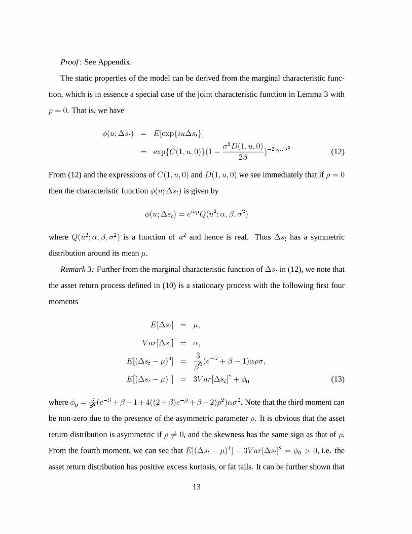
The static properties of the model can be derived from the marginal characteristic func-
tion, which is in essence a special case of the joint characteristic function in Lemma 3 with
R ' f. That is, we have
�E�( {r � � ' .di Ti��{r � jo
' i Ti�E�c �c f�jE�� j�(E�c �c f�
2q�� � 8O4�2 : �
(12)
From (12) and the expressions of �E�c �c f� and (E�c �c f� we see immediately that if 4 ' f
then the characteristic function �E�( {r � � is given by
�E�( {r � � ' e� )$P'E�
�(kc qc j
��
where 'E��(kc qc j
�� is a function of �
�and hence is real. Thus {r � has a symmetric
distribution around its mean >.
Remark 3: Further from the marginal characteristic function of {r � in (12), we note that
the asset return process de¿ned in (10) is a stationary process with the following ¿rst four
moments
.d{r � o ' >c
T @od{r � o ' kc
.dE{r � � >�Qo '
�
q� Ee �14 n q � ��k4jc
.dE{r � � >�Ro ' �T @od{r � o
�n � � (13)
where � � 'Q4�S Ee
�14nq��neEE2nq�e
�14nq�2�4
��kj
�. Note that the third moment can
be non-zero due to the presence of the asymmetric parameter 4. It is obvious that the asset
return distribution is asymmetric if 4 9' f, and the skewness has the same sign as that of 4.
From the fourth moment, we can see that .dE{r � � >�Ro � �T @od{r � o
�' � � : f, i.e. the
asset return distribution has positive excess kurtosis, or fat tails. It can be further shown that
13

the distribution of asset returns {r � is leptokurtic, more peaked in the vicinity of its mean
than the distribution of a comparable normal random variable. These features are consistent
with the empirical ¿ndings on the unconditional distributions of many ¿nancial asset returns.
Remark 4: From the joint characteristic function in Lemma 3, we can readily calculate
various cross moments of {r � . In particular, we have (i) the mean adjusted asset return
{r � � > is uncorrelated over time, i.e.
.dE{r � � >�E{r ����� � >�o ' fc � : �
and (ii) the squared mean adjusted asset return E{r � � >��
is correlated over time with,
�J�dE{r � � >��c E{r ����� � >�
�o
'�
2qQ e �
? �$� � A 4Ee4 � ��Ee
4 � � n e4�Ee4 � q � ���kj
�c � : � (14)
which is strictly positive but decreases with � and goes to f as � goes to n4. Thus, while
the asset returns are uncorrelated over time, the squared asset returns are autocorrelated. We
also note that the squared return process can behave quite differently than the instantaneous
volatility process.
The discussion and derivations surrounding Example 2 above highlights the fact that
often in af¿ne diffusions with latent variables can we exploit the form of the characteristic
functions, both conditional and unconditional, to examine the statistical properties of these
processes. In the next section, we will see that the joint characteristic function can also be
used to develop ef¿cient estimators of the parameters in AD and AJD models, especially for
the case that some of the state variables are unobserved or latent.
14
3 GMM and Empirical Characteristic Function (ECF) Es-
timation of the Continuous Time Stochastic Processes
In this section, we focus on the estimation of the af¿ne jump-diffusion process as de¿ned
in (1) that involves latent variables, especially the case that the observed partial process
is non-Markovian. The processes without latent variables can be viewed as special cases,
which have been intensively studied in Singleton (1999). For the case that the conditional
characteristic function of the af¿ne diffusion or af¿ne jump-diffusion process f � has explicit
analytical form and the whole vector of f � is observable, Singleton (1999) proposes both
the maximum likelihood (ML) estimation and partial maximum likelihood (PML) estima-
tion based on Fourier inversion of the conditional characteristic function (CCF), as well as
the standard quasi-maximum likelihood (QML) estimation based on conditional moments.
Singleton (1999) also proposes both the ef¿cient and approximately ef¿cient estimation of
the AD or AJD process f � based directly on the empirical conditional characteristic function
(ECCF). As will be seen later in this section, the basic idea is to match the analytical CCF
to the empirical CCF. For the ef¿cient estimation, however, the optimal weight function is
not known as it cannot be computed without a prior knowledge of the conditional density
function, which we will also discuss in detail later in this section. When part of the state
variables of f � is unobserved or latent, Singleton (1999) proposes the simulated method
of moments (SMM) estimation based on the CCF, which involves simulating the stochastic
process. Since the model is essentially in continuous time, such simulation often involves
approximation error due to the discretization of the data generating process (DGP). Chacko
and Viceira (1999) construct a GMM estimator based on the unconditional mean of the dif-
ference between the empirical characteristic function and analytical characteristic function
for integer values of the dummy variable �. 2 However, their procedure does not utilize
2We wish to thank the anonymous referees for bringing our attention to this research.
15

the full conditioning information in the data, and therefore while their estimation example
is truly exact, the lack of conditioning information produces an estimator that is neither as
ef¿cient as that in Singleton (1999) nor as the estimators we shall propose in this section.
Estimation of dynamic nonlinear latent variable models, such as the SV model in (10),
is by no means a trivial task. The dif¿culty arises due to the fact that the latent variables,
i.e. the stochastic volatility in the case of the SV model, are unobservable, and thus the
models cannot be estimated using standard maximum likelihood (ML) methods as the la-
tent or unobserved variable has to be integrated out of the likelihood.3 Over the past few
years, however, remarkable progress has been made in the ¿eld of statistics and economet-
rics regarding the estimation of nonlinear latent variable models in general and SV models in
particular. Various estimation methods have been proposed for SV models, which are mostly
simulation-based, computationally intensive and involve discretization when applied to the
continuous-time processes. For example, we have the Quasi Maximum Likelihood (QML)
by Harvey, Ruiz and Shephard (1994), the Monte Carlo Maximum Likelihood by Sandmann
and Koopman (1997), the Markov Chain Monte Carlo (MCMC) methods by Jacquier, Polson
and Rossi (1994) and Kim, Shephard and Chib (1998) for discrete-time SV models, and the
Ef¿cient Method of Moments (EMM) by Gallant and Tauchen (1996) for both discrete-time
and continuous-time SV models. Applications of EMM have been performed by Gallant,
Hsieh and Tauchen (1997), Andersen and Lund (1997) to symmetric continuous-time SV
models, and Andersen, Benzoni and Lund (1998) and Chernov and Ghysels (1999) to asym-
metric continuous-time SV models. To our knowledge, there have been very few attempts
to estimate the continuous-time model as speci¿ed in (10) with non-zero correlation be-
tween asset returns and conditional volatility (i.e. 4 9' f). In addition to the aforementioned
3This is not a standard problem since the dimension of this integral equals the number of observations,
which is typically large in ¿nancial time series. Standard Kalman ¿lter techniques cannot be applied due to the
fact that either the latent process is non-Gaussian or the resulting state-space form does not have a conjugate
¿lter.
16

EMM applications, Singleton (1999) applies the proposed simulation based ECF estimator
for af¿ne diffusion models to the SV model as de¿ned in (10) using the S&P 500 index re-
turns. Chacko and Viceira (1999) apply their GMM estimation to the jump-diffusion process
with stochastic volatility using both weekly and monthly total return observations on the
CRSP value-weighted portfolio.
In this paper, we exploit the fact that the characteristic function of the asset return pro-
cess as well as the joint asset return process can often be derived analytically. Using these
analytical results, we propose the following two different methods for the estimation of the
continuous-time SV process, one is the generalized method of moments (GMM) based on
the exact moment conditions and the other is the empirical characteristic function (ECF)
method which matches the empirical characteristic function calculated from the data to the
analytical characteristic function derived from the model. As in Singleton (1999), for the
estimators discussed in this section, we assume that Hansen’s (1982) regularity conditions
are satis¿ed.
3.1 GMM Estimation of the Continuous Time Stochastic Processes
As shown in Section 2, various unconditional moments of the state variables can be derived
from the unconditional joint characteristic function. These moments are exact in the sense
that they are corresponding to the continuous time DGP without any discretization or approx-
imation. When the joint characteristic function has a closed analytical form, these moment
conditions also have explicit expressions whenever they exist. Consequently, these moment
conditions can be used to estimate the stochastic processes following a standard GMM pro-
cedure. In this section, we present this procedure for the case that the partial process 7 � of
f � is observed and ¿rst difference stationary, and the rest of the process is latent. For other
cases, the only difference is the change of notation. Let �E� � c ��c � � c ��c � ���� c ����%� � ({r � c ��c
{r � c ��c{r ���� c ��c{r�$� � � be the unconditional joint characteristic function of i{r � c ��c{r � c ��c
17
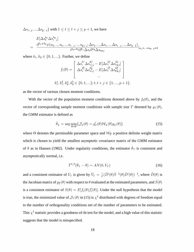
{r ���� c ��c{r�%� � j with � � | � | n � � R n �, we have
.d{r& �� {r
& ����� o
'Y& �G� & �
�E� � c ��c � � c ��c � ���� c ��c ��%� � ( {r � c ��c{r � c ��c{r ���� c ��c{r�%� � ��& �G� & � Y
& � {r � Y& � {r ����
m ) �B� T T T � ) � " �G�K�
where & � c & � 5 ifc �c ���j. Further, we de¿ne
s � Ew� '
5
9
9
9
7
{r&MU�� {r
&MU����� �.d{r&MU�� {r
&%U����� o{r
&MV�� {r&MV����� �.d{r
&MV�� {r&%V����� o
���
6
:
:
:
8
& W� c &X� c & W� c &
X� 5 ifc �c ���j( |c |n � 5 i�c ���c Rn �j�
as the vector of various chosen moment conditions.
With the vector of the population moment conditions denoted above by s � Ew�, and the
vector of corresponding sample moment conditions with sample size A denoted by } Y Ew�,
the GMM estimator is de¿ned as
w Y ' @h}4�?ZN[9\ iM Y Ew� ' }�Y Ew�Z Y Ew�} Y Ew�j (15)
where X denotes the permissible parameter space and Z Y a positive de¿nite weight matrix
which is chosen to yield the smallest asymptotic covariance matrix of the GMM estimator
of w as in Hansen (1982). Under regularity conditions, the estimator w Y is consistent and
asymptotically normal, i.e.
A�]2 �
Ew Y � w� � ��Efc T Y � (16)
and a consistent estimator of T Y is given by T Y '�Y E (
�Ew� 7
���Ew� (
�Ew��
��� , where (Ew� is
the Jacobian matrix of } Y Ew�with respect to w evaluated at the estimated parameters, and 7Ew�
is a consistent estimator of 7Ew� ' .ds � Ew�s�� Ew�o� Under the null hypothesis that the model
is true, the minimized value of M Y Ew� in (15) is ��
distributed with degrees of freedom equal
to the number of orthogonality conditions net of the number of parameters to be estimated.
This ��
statistic provides a goodness-of-¿t test for the model, and a high value of this statistic
suggests that the model is misspeci¿ed.
18

3.2 ECF Estimation of the Continuous Time Stochastic Processes
Before we discuss the estimation of the AD and AJD model via the ECF, it is worthwhile
to brieÀy outline the ECF estimation method for stationary stochastic processes. Suppose a
vector of random variables + has the distribution function 8 E+( w� where w 5 X the parameter
space which speci¿es the distribution, the characteristic function is de¿ned as the Fourier
transformation of the distribution function. In particular, the joint characteristic function of
+, denoted by �E�( +c w�, is de¿ned as
�E�( +c w� ' .di Ti���+jo '
]
i Ti���+j_8 E+( w� (17)
and the joint empirical characteristic function, denoted by � � E�( +�, of the random vector +
is the sample counterpart of the characteristic function,
� � E�( +� '�
?
�[
I� �i Ti��
�+ j '
]
i Ti���+j_8 � E+( w� (18)
where 8 � E+� is the empirical distribution function. Since there is an unique Fourier-Stieltjes
transformation, the joint characteristic function and the joint empirical characteristic func-
tion de¿ned above contain the same amount of information as the distribution function and
the empirical distribution function (i.e. the sampling observations) respectively. The basic
idea of the empirical characteristic function estimation method for time series models was
¿rst proposed by Feuerverger (1990) by extending his earlier results on the ECF method
(see Feuerverger and McDunnough (1981) and Feuerverger and Mureika (1977)) to estimate
stationary stochastic processes. He proposed splitting the data into ? ' A � R overlapping
blocks, each of length R n �, and using the joint characteristic function of each block to
estimate the parameter vector w by minimizing the following weighted distance 4
4�?Z]
���]
m �E�( +c w�� � � E�( +� m�)E��_� (19)
4Alternatively, one can de¿ne the distance as a summation of the squared difference between the analytical
characteristic function and empirical characteristic function over a discrete set of x.
19

or, under standard regularity conditions, solving the ¿rst order conditions of the above opti-
mization problem
]
���]
E�E�( +c w�� � � E�( +���E�c w�_� ' f (20)
where �E�( +c w� and � � E�( +� are given in (17) and (18) and + ' E% c %E� � c ���c %E�^� �, � '
�c 2c ���c ? ' A � R with % being observations on the time series. Both )E�� and �E�� are
weight functions. Since (20) is the ¿rst order conditions of (19), for these two procedures to
be equivalent it is necessary for �E�� to be a function of w as it involves the derivative of �E��
with respect to w. As �E�( +c w� is a function of the unknown parameters, i.e., w and � � E�( +�
a function of the data, the ECF method merely minimizes (19) with respect to w� Feuerverger
(1990) also showed that using (20) with �E�c w� chosen as
�E�c w� '�
E2Z��%� �]
� � �] Y *? sE% m% _��� c ���c % _�@� �
Ywi TE��� * + �_+
results in an estimator asymptotically equivalent to maximum likelihood. Lemma 4 gives the
asymptotic distribution associated with the ECF estimator derived from (19).
Lemma 4. The parameter estimators w obtained from the empirical characteristic func-
tion method is consistent and asymptotically normally distributed with
s?Ew � w�
`�$ �Efcl� (21)
where l ' ����Ew��Ew��
���Ew� is the variance-covariance of the parameter estimators with
both �Ew� and �Ew� de¿ned in the Appendix, and a consistent estimator of the variance-
covariance is also given in the Appendix.
Proof : See Appendix.
In section 2 we noted that for the AD and AJD models, the joint characteristic function
often has a closed form. This expression can be used in the above outlined estimation strategy
to develop relatively ef¿cient estimators of the unknown parameters.
20

In the full Markov model where all variables are observed, our proposed estimator will be
an alternative to those proposed in Singleton (1999) and Chacko and Viceira (1999). Both
these papers use the conditional characteristic function rather than the joint characteristic
function, with the Singleton (1999) approach making full use of the conditioning informa-
tion. The major difference between our approach and the approach in Singleton (1999) is
that instead of conditioning on the initial observation, our approach includes the initial ob-
servation in the joint unconditional distribution. With large sample size and for the Markov
models, the approaches would be equivalent as it is clear that we would simply need blocks
of length two. Therefore, in situations where all variables in the model are observed we rec-
ommend the use of the Singleton (1999) GMM-CCF estimator or our estimator with block
size of two, or R ' �. Singleton’s (1999) estimator uses a ¿nite grid of points for the esti-
mation of the conditional characteristic function and his estimator hinges on the choice of
the number of points and their value. Our estimator with R ' � only requires the choice
of the weight function )E��. How these estimators compare in ¿nite samples and how they
perform for different models are important and interesting issues. However, these issues are
beyond the scope of this paper and will be examined in a separate Monte Carlo study.
As we mentioned in the introduction, the more challenging estimation problem arises
for the AD and AJD models where some of the variables are unobserved or latent. In this
case, the dif¿culty arises with the estimation methods based on the conditional characteristic
function as not all the conditioning information is observed. These unobserved state vari-
ables therefore need to be integrated out. The issue is further complicated when the observed
state variables, as part of the whole state variables which are Markovian, are not necessarily
Markovian. That is, the future states may depend on not only the current states but also their
past and in some cases even the entire history. This situation can be handled with our esti-
mator and was also a subject of discussion in both Chacko and Viceira (1999) and Singleton
(1999). Chacko and Viceira’s (1999) strategy is to ¿rst examine the conditional characteristic
21

function and then to integrate out the conditioning information resulting in the marginal or
unconditional characteristic function, from which moment conditions and a GMM estimator
are derived. Unfortunately, the marginal characteristic function is unable to help explain any
time series behavior in the observed process. Singleton’s (1999) approach relies on simula-
tion methods to integrate out the dependence of the conditional characteristic function on the
unobserved or latent variables. However, it could be argued that the use of simulation along
with discretization of the continuous-time process seems to negate the tractability arguments
associated with the af¿ne AD and AJD models in terms of their characteristic functions.5
The proposed estimators in this paper, both the GMM and ECF, exploit the known form
of the joint unconditional characteristic function. As shown in Section 2, the joint uncondi-
tional characteristic function often has closed analytical form for the AD and AJD models,
thus (19) or (20) can be readily used for the estimation of the processes. One of the advan-
tages of the estimators proposed in this paper is that they are exact approaches, in the sense
that they require neither discretization nor simulation. More speci¿cally, in the GMM case
we are able to use both marginal and joint moment conditions resulting in a parsimonious,
powerful and intuitive GMM procedure. The ECF estimator is also appealing as it essen-
tially performs GMM with a continuum of moment conditions and has the added property
of relative ef¿ciency. When the weight function is asymptotically optimal, the ECF method
has the same asymptotic ef¿ciency as the ML estimation method. Furthermore, the joint
unconditional characteristic function reÀects both the static and time series behavior of the
observed process. As will be discussed later in this section, for Markov process, it is suf¿-
cient to have block size of two, or R ' �, in the estimation. While for non-Markov process,
it would appear that there is no general solution to the choice of the block size.
We will conclude this section by examining in some detail the Singleton (1999) empirical
conditional characteristic function (ECCF) estimator for Markov models, showing how it
5We thank one of the referees for this argument.
22

can be extended to non-Markov models and how easily it can be adapted to generate the
exact ML estimator rather than the conditional ML estimator. More speci¿cally, Singleton’s
(1999) results exploit the particular dependency in Markov models resulting in the following
optimal estimating equations, similar to (20), which result in conditional MLE:Y[
I� �
]
�E�c wm%N�K� �Ee � )$+%a � �E�m% _��� ��_� ' f
where
�E�c wm%N�K� � ' �
2Z
] Y *? sE% m%_��� �Yw
e� )$+Ma
_%
and
�E�m%_��� � ' .de� )$+%a m% _��� o�
The following Lemma extends some of the ideas in Singleton (1999) to non-Markov
models and gives the optimal estimating equations which result in exact Maximum Likeli-
hood estimators.
Lemma 5. For a general stationary stochastic process with the conditional likelihood
given by
u ��\
I� �sE% mU _��� �
where U _��� signi¿es information up to and including time � � �, the optimal weight function
associated with observation �, is given by
� E�c wmU _��� � ' �
2Z
]
e�1� )$+%a Y *? sE% mU N��� �
Yw_% (22)
and the resulting estimating equations leading to the conditional MLE are:�[
I� �
�]
� E�c wmU _��� �e � )$+ a _��
' f (23)
For exact MLE we need to amend the estimating equations to take into account the additional
information in the marginal pdf of % � , i.e., sE% � �. The estimating equations become:
]
� � E�c w�e �)$+ �
_% � n�[
I� �
]
� E�c wmU _��� �e � )$+Ma _% ' f (24)
23

with
� � E�c w� '�
2Z
]
e� � )$+ � Y *? sE% � �
Yw_% � (25)
Proof : See Appendix.
If the process is Markov, then
sE% mU _��� � ' sE% m%_��� �
and unlike in the general case, this pdf maintains a constant form since the information set is
now just the E������L observation. Consequently, the weight function will also be of constant
form, viz.,
� E�c wmU N�K� � ' � � E�c wm% _��� �c ;� : 2
When the conditional density is unknown but the process is Markov we can obtain an ap-
proximation to the optimal weight function by approximating the *? sE% m%N��� �, e.g. via an
Edgeworth expansion. This approach is currently under investigation by the authors.
However, when the process is not Markov and sE% mU _��� � is not known we cannot use
the Edgeworth approach as the form of sE%mU N��� � is not constant. Consequently, we have no
alternative but to use some simulation approach along with the ECF as in Singleton (1999) or
use the weighted function of the integrated MSE given by (19). Using (19) raises the issues
of the dimension of the joint characteristic function, i.e., the length of the overlapping blocks
given by ERn �� and the choice of the weight function )E��.
Unfortunately, it would appear that there is no general solution to the choice of R or
)E��, except perhaps in a Markov model where R ' � is clearly suf¿cient to capture the
dependency in the data. Consequently, optimal values for R and )E�� need to be considered
on a case by case basis.
24

4 An Empirical Application: Estimation of the Stochastic
Volatility (SV) Model
In this section, an empirical application of the proposed methods in section 3, namely the
ECF method and GMM, is undertaken for the SV model as de¿ned in (10), namely
_r � ' >_|n T�32 �� _` �
_T � ' qEk� T � �_|n jT�32 �� _` ;�
_` � _` ;� ' 4_|c | 5 dfc A o (26)
The data set in our application consists of the daily S&P 500 index returns over the period
from 1990 to 1999, obtained from DataStream International. The summary statistics of
the static and dynamic properties of daily S&P 500 index returns are reported in Table 1,
from which we can see that the daily index returns are skewed with excess kurtosis. As
for the dynamic properties, the autocorrelations of index returns are in general low. For the
squared return series, the ¿rst order autocorrelation is low but not negligible, and higher
order autocorrelations are overall diminishing.
The GMM estimation, as proposed in section 3, is based on both the marginal and joint
moment conditions of the observed return process {r � which is shown to be stationary.6
There are obviously in¿nite number of moments that may be used in GMM estimation. The
primary guidance of the moment selection in this paper is the Monte Carlo evidence in An-
dersen and Sørensen (1996) on the GMM estimation of a discrete-time SV model. Firstly, in
determining the number of moments used in the estimation, we keep in mind the following
fundamental trade-off: inclusion of additional moments improves estimation performance
for a given degree of precision in the estimation of the weight matrix, but in ¿nite sam-
6GMM is also used by Andersen (1994), Andersen and Sørensen (1996) to estimate discrete-time SV mod-
els and Ho, Perraudin and Sørensen (1996) to estimate a continuous-time SV model with different speci¿cation
of the volatility process.
25
ples this must be balanced against the deterioration in the estimate of the weight matrix as
the number of moments increases. Secondly, very high order moments should be avoided
due to their erratic ¿nite sample behavior caused by the presence of fat tails in the asset
return distribution. Asymptotic normality of the GMM estimator requires ¿nite variance of
the moment conditions and good estimates of these quantities in ¿nite samples. Thus our
moment selection tends to focus on the lower order moments, which is consistent with An-
dersen and Sørensen (1996) and Jacquier, Polson and Rossi (1994). Thirdly, different from
the discrete-time SV model, the absolute moments of the asset returns can not be derived for
the continuous-time model. The Monte Carlo evidence in Andersen and Sørensen (1996),
however, suggests that inclusion of these kinds of moments is in general unlikely to improve
estimation performance and at best the gains are quite minor.
The exact moment conditions are chosen with further considerations of the particular
model. First of all, since stochastic volatility allows for skewness and excess kurtosis,
the ¿rst four unconditional moments are important. Secondly, since the autocorrelation of
squared returns is determined by the SV process and its correlation with asset returns, the
joint moments of the squared returns are important for the identi¿cation of the SV process.
As the autocorrelation is varying over time, we use these moment conditions with different
lags. Consequently, the moments included in the GMM estimation consist of the ¿rst four
unconditional moments of the asset returns and the ¿rst ¿ve orders of autocorrelation of the
squared returns. The weight matrix is estimated by the Barlett kernel proposed by Newey
and West (1987) with a ¿xed lag length of 20. The starting values are set as the method of
moments estimates of the parameters, which are obtained by matching the ¿rst four uncon-
ditional moments and the ¿rst order autocorrelation of the squared returns to the data.
The ECF estimation is also based on the time series observations of index returns {r � .
We note that while the bivariate stochastic process ir � c T � j is a Markov process by the
continuous-time model speci¿cation, the marginal process ir � j and the return process i{r � j
26

are non-Markovian. Due to the lack of the exact optimal weight function in (20), our estima-
tion is based on the minimization problem in (19) with the weight function being the pdf of
a multivariate normal distribution with zero mean and variance-covariance matrix P ' j�� U ,
namely )E�� '�s ?��3b : ��A � i Ti�
) * )� : ��j. As we have pointed out in the general discussion of
the ECF method, for non-Markovian processes there are no general solutions for the choice
of optimal weight function )E�� or the block size R. A practical solution for the choice of
optimal weight function is to use the idea in the GMM procedure, i.e. choosing the weight
function that minimizes the variance of the parameter estimates. In our particular choice of
the weight function, it amounts to choosing the value of j � . The choice of the block size R is
more complicated, depending on the exact structure of the DGP. For instance, for an AR(^)
process we have that asymptotic ef¿ciency will be achieved with R set to ^ (see Knight and
Yu (2000)). However, for an invertible MA(^) process, which is in essence an AR(4), it
is clear that we need as large as possible block size to achieve asymptotic ef¿ciency. For
a general non-linear process, increasing the block size should in principle lead to gains in
asymptotic ef¿ciency, however, it also can substantially increase the computational burden
in the estimation. Thus, in general there is a trade-off between large blocks for asymptotic
ef¿ciency and small blocks for computational ef¿ciency. In addition, we note that with ¿xed
sample size, increasing the block size will reduce the number of sampling blocks in the ECF
estimation. In our application, to highlight the effect of varying block size and to ease the
computational burden, we consider, in the ECF estimation, ¿ve different block sizes of two
to six, i.e. R ' �c 2c �c e, and D. With R ' D, the block size exceeds the span of one week
period. The starting values of the parameters in the ECF estimation are also set as the method
of moments estimates of the parameters.
Table 2 reports the parameter estimates and asymptotic standard errors for the SV model
based on different estimation methods. For the ECF estimation, we only report for each R the
parameter estimates using the multivariate normal pdf as weight function, with the standard
27

deviation parameter chosen among various values to minimize the variance of parameter es-
timates. Firstly, the SV model has a reasonable ¿t to the S&P 500 index returns over the
sample period. The Hansen-J ��
test statistic for the model speci¿cation based on GMM
estimation has a p-value of f�eDH.7 Secondly, in both the GMM and ECF estimation, the
estimate of q is in general signi¿cant, suggesting there exists mean reversion in the volatility
process. Thirdly, the ECF estimates are in general sensitive to the choice of block size R.
While the estimate of the expected asset return > and that of the long run mean of volatility
k (orsk) are relatively stable, the estimates of parameters reÀecting the dynamic proper-
ties of the model are, as expected, varying with different values of R and have relatively
larger standard errors. In particular, the mean reversion parameter q has estimates that range
from f�2�e to f����, and the asymmetric correlation parameter between the asset return and
stochastic volatility has estimates that range from �f�2ee to �f�2.�.
Many other estimation methods proposed for the dynamic latent variable model have
also been applied to the SV model, mostly using the S&P 500 index returns as well. For in-
stance, Andersen, Benzoni, and Lund (1998) and Chernov and Ghysels (1999) estimated the
SV model using EMM based on daily S&P 500 index returns from 1980 to 1996 and from
November 1985 to October 1994 respectively. Singleton (1999) estimated the SV model
using SMM based on daily S&P 500 index returns over the period of 1990 to 1997.8 Chacko
and Viceira (1999) and Pan (1999) also estimated the SV model using weekly or monthly
asset returns. In these studies, the data source, sampling period, or the drift function speci¿-
7Based on the data set that includes the 1987 market crash, the SV model has rather poor ¿t to the S&P500
index returns and the GMM estimation reports a much smaller p-value for the Hansen-J " c test statistic, sug-
gesting that it is dif¿cult for the SV model to generate large random jumps as in the case of 1987 market crash.
Inclusion of the ¿fth moment of asset returns in the GMM estimation also signi¿cantly decreases the p-value
of the Hansen-J " c test statistic, which is a result of either the erratic ¿nite sample behaviour caused by the
presence of fat tails in the asset return distribution or the inability of the SV model to match the ¿fth moment
of the observed process or the combination of both.8In the simulation of sampling path, 50 subintervals per day are used in simulating 50,000 daily observations
following the Euler discretization scheme.
28

cation varies from one to another. Overall, our estimation results based on the daily S&P500
index returns over the period of 1990 to 1999 are very comparable to the SMM estimates
in Singleton (1999). Noticeable difference between our estimation results and those ob-
tained by EMM is the value of the mean reversion parameter and the conditional variance of
the volatility process. Our estimation results indicate a much stronger mean reversion and
higher volatility for the stochastic volatility process. An intuitive justi¿cation is that, in the
SV model framework, in order to incorporate the negative skewness and fat tails of the S&P
500 index return distribution, a negative correlation between asset return and volatility and a
signi¿cant level of variation in the stochastic volatility are required. It is also noted that the
parameters in the SV process are tied to each other as the unconditional mean and variance
of the volatility are given respectively by k and k: �� 4 . It is easy to see that given k (the long-
run mean of volatility) and the variance of the volatility, a high value of j will induce a high
value of q and vice versa.
A systematic comparison of the ¿nite sample properties of alternative estimators, in-
cluding the ones proposed in this paper, calls for a Monte Carlo simulation study. Due to
the intensive computation involved in some of the estimation methods, especially the EMM
approach, this task will not be pursued in this paper but in a separate study. To gauge the
performance of our estimators, however, we investigate the implications of the parameter
estimates on the static and dynamic properties of the underlying process. Intuitively, when
the basic statistical properties of the estimated model are not consistent with those of the
data, the following conclusions are in order: either the model is a poor candidate of the DGP
or the estimation method employed has less desirable ¿nite sample properties. Based on this
intuition, we exploit the analytical moments derived from the model to calculate the major
summary statistics from alternative parameter estimates. Table 3 presents the exact uncondi-
tional moments calculated from various parameter estimates, together with those calculated
from the data. Overall, the GMM and ECF estimates provide the skewness and kurtosis of
29

asset returns and the standard deviation of squared returns that are very close to their data
counterparts. As expected, the increase of block size R does not signi¿cantly improve, if not
hurt, the model’s ability to capture the static properties of the data. Figure 1 further plots the
¿rst twenty orders of autocorrelations of the squared returns calculated from various param-
eter estimates, together with those calculated from the data. The GMM and ECF estimates
all generate a relatively high ¿rst order autocorrelation with higher orders of autocorrela-
tions quickly vanishing. For the ECF estimates, as R increases from � to D, it is expected
that the model can better capture the dynamic property of the data. As shown in Figure 1,
the ¿rst ¿ve orders of autocorrelation of squared asset returns calculated from the ECF es-
timates appear to ¿t those calculated from the data reasonably well. However, the structure
of the correlogram of the squared asset returns generated from the model is not successful
in matching its counterpart of the data. More speci¿cally, the correlogram of squared asset
returns generated by the model is strictly monotonically decreasing, but the correlogram of
squared asset returns calculated from the data, while overall decreasing, is not monotonic.
5 Conclusion
Concerning the statistical properties and the estimation of AD and AJD models, this paper
has made several contributions. Firstly, we have shown how the joint characteristic func-
tion can be derived for AD and AJD models and thus enabling various statistical properties
of these processes to be examined. As an illustration, from the joint characteristic func-
tion of asset returns, we derived analytically the exact static and dynamic properties of the
continuous-time square-root SV process. Secondly, using the joint characteristic function we
propose alternative estimators, both GMM and ECF, for these Markov AD and AJD models.
More importantly, we show how in the latent variable case these estimators are both compu-
tationally ef¿cient and asymptotically relatively ef¿cient. The estimation is based on exact
30
moment conditions or exact joint characteristic function and requires neither discretization
of the continuous-time process nor simulation of the sampling path. Finally, the illustrative
examples, in particular the SV model, have demonstrated the usefulness and elegance of the
proposed techniques. The empirical application of the SV model using the S&P 500 index
returns demonstrates that both the ECF and GMM estimation procedures not only are easy
to implement and computationally ef¿cient, but also have nice ¿nite sample properties.
31
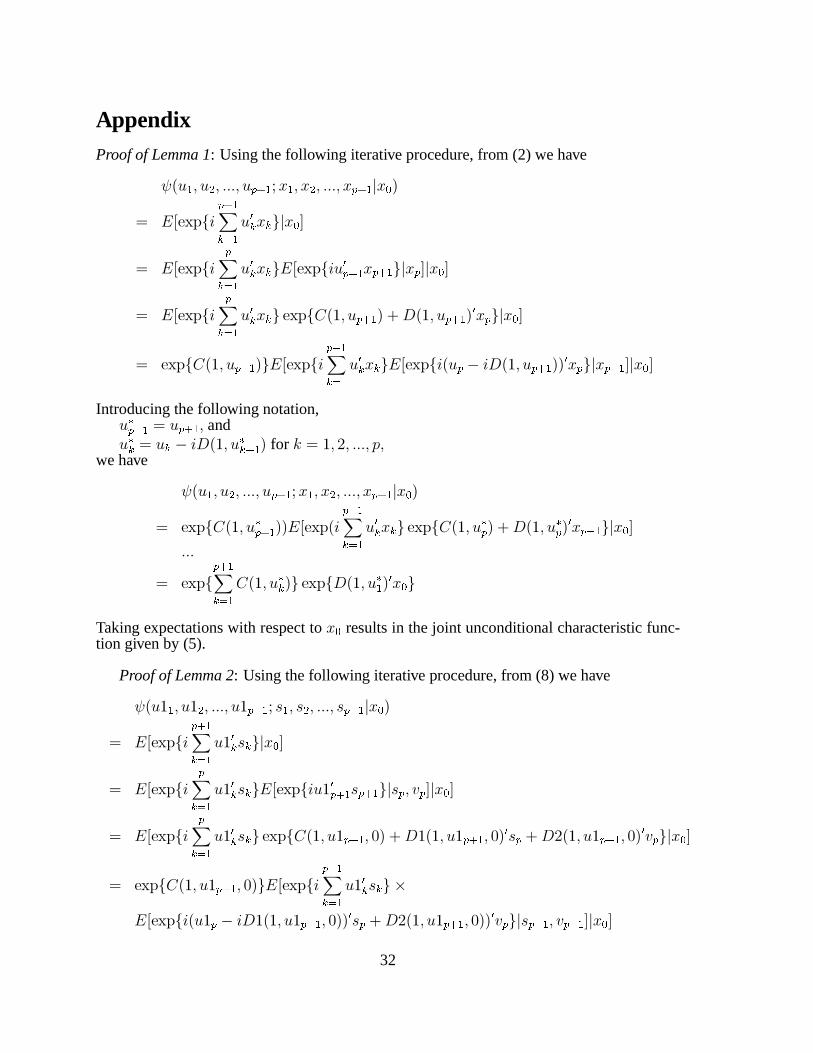
AppendixProof of Lemma 1: Using the following iterative procedure, from (2) we have
�E� d c � e c ���c �f$g'd ( % d c % e c ���c %f$g d m% h �
' .di Ti�f%g d[
iMj d� k i % i jm% h o
' .di Ti�f[
iMj d� k i % i j.di Ti�� kf$g d %f%g d jm%f om% h o
' .di Ti�f[
iMj d� k i % i j i Ti�E�c �f%g d � n(E�c �f$g d � k %f jm% h o
' i Ti�E�c �f$g'd �j.di Ti�fOlKd[
iNj d� k i % i j.di Ti�E�f � �(E�c �f$g'd �� k %f jm%fOlKd om% h o
Introducing the following notation,� mf%g d ' �f$g d c and� mi ' � i � �(E�c � mi g d � for & ' �c 2c ���c Rc
we have
�E� d c � e c ���c �f%g d ( % d c % e c ���c %f%g d m% h �
' i Ti�E�c � mf%g d ��.di TE�f�l�d[
iMj d� k i % i j i Ti�E�c � mf � n(E�c � mf � k %f�l�d jm% h o
���
' i Tif$g d[
iNj d�E�c � mi �j i Ti(E�c � m d � k % h j
Taking expectations with respect to % h results in the joint unconditional characteristic func-tion given by (5).
Proof of Lemma 2: Using the following iterative procedure, from (8) we have
�E�� d c �� e c ���c ��f$g'd ( r d c r e c ���c rf%g d m% h �
' .di Ti�f$g d[
iNj d�� k i r i jm% h o
' .di Ti�f[
iNj d�� k i r i j.di Ti��� kf$g'd rf%g d jmrf c �f om% h o
' .di Ti�f[
iNj d�� k i r i j i Ti�E�c ��f%g d c f� n(�E�c ��f$g d c f� k rf n(2E�c ��f%g d c f� k �f jm% h o
' i Ti�E�c ��f$g d c f�j.di Ti�f�l�d[
iMj d�� k i r i j �
.di Ti�E��f � �(�E�c ��f$g d c f�� k rf n(2E�c ��f%g d c f�� k �f jmrf�l�d c �fOl�d om% h o
32

Introducing the following notation:�� mf ' ��f c �2 mf ' fc and�� mi ' �� i � �(�E�c �� mi g d c �2 mi g d �c �2 mi ' ��(2E�c �� mi g'd c �2 mi g d � for & ' �c 2c ���c R,
we have
�E�� d c �� e c ���c ��f$g d ( r d c r e c ���c rf%g d m% h �
' i Ti�E�c �� mf%g d c �2 mf$g d �j.di Ti�fOl�d[
iNj d�� k i r i j �
i Ti�E�c �� mf c �2 mf � n(�E�c �� mf c �2 mf � k rf�l�d n(2E�c �� mf c �2 mf � k �f�l�d jm% h o���
' i Tif$g d[
iNj d�E�c �� mi c �2 mi j� i Ti(�E�c �� m d c �2 m d � k r h n(2E�c �� m d c �2 m d � k � h j
Taking expectations with respect to % h results in the unconditional joint characteristic func-tion given in (9).
Proof of Lemma 3: Applying the results of Lemma 2 directly to the SV model, we derivethe joint characteristic function of {r d ' r d �r h c{r e ' r e �r d c ���c and {rf%g d ' rf%g d �rf cwhere R � �, i.e.,
�E� d c � e c ���c �f$g d ( {r d c{r e c ���c{rf%g d �' .di Ti�� d {r d n �� e {r e n ���n ��f%g d {rf%g d jo' .d.di Ti�� d {r d n �� e {r e n ��n ��f%g d {rf$g'd j m rf c �f oo' .di Ti�� d {r d n �� e {r e n ��n ��f {rf n �E�( �f$g d c f� n(E�( �f$g d c f��f jo
Introducing the following notation,�� mf%g d ' �f$g d c �2 mf$g'd ' f�� mi ' � i c �2 mi ' ��(E�(�� mi g d c �2 mi g d � for & ' �c ���c R,
we have
�E� d c � e c ���c �f$g d ( {r d c{r e c ���c{rf%g d �
' i Ti�E�( �� mf%g d c �2 mf%g d �j.di Ti�f[
iMj d� i {r i n(E�( �� mf$g d c �2 mf$g'd ��f jo
���
' i Tif%g d[
iMj d�E�( �� mi c �2 mi �j.di TiE
f%g d[
iMj d(E�( �� mi c �2 mi ��� h jo
Taking expectations with respect to � h which follows a Gamma distribution, we have
�E� d c � e c ���c �f$g d ( {r d c{r e c ���c{rf%g d �
' i Tif%g d[
iMj d�E�( �� mi c �2 mi �j � E�� j
e
2q
f%g d[
iMj d(E�( �� mi c �2 mi �� l�eBn9oCp]q5r
33
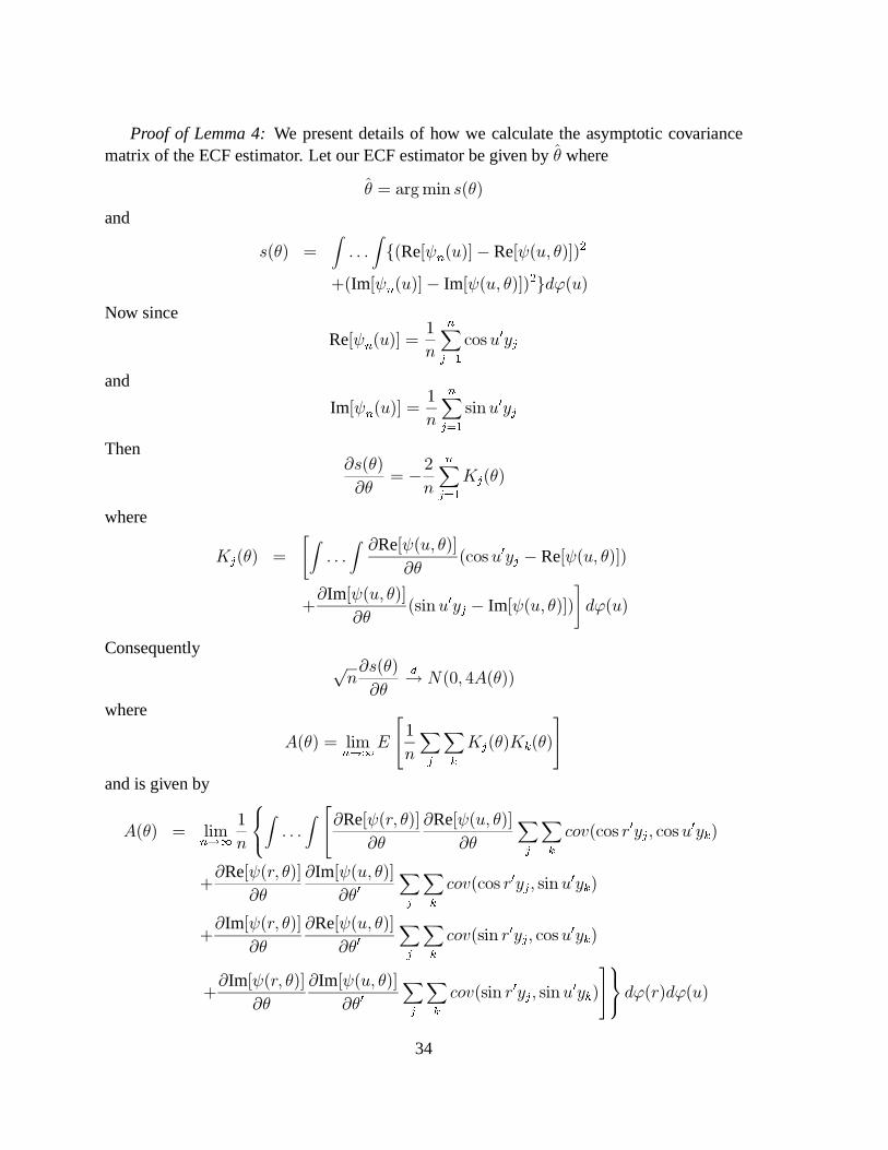
Proof of Lemma 4: We present details of how we calculate the asymptotic covariancematrix of the ECF estimator. Let our ECF estimator be given by w where
w ' @h}4�? rEw�
and
rEw� ']
� � �]
iERed� s E��o� Red�E�c w�o�e
nEImd� s E��o� Imd�E�c w�o�e j_)E��
Now since
Red� s E��o '�
?
s[
t j dULt� k +t
and
Imd� s E��o '�
?
s[
t j dt�?� k + t
ThenYrEw�
Yw' �2
?
s[
t j dg t Ew�
where
g t Ew� '
%
]
� � �] YRed�E�c w�o
YwEULt � k + t � Red�E�c w�o�
nYImd�E�c w�o
YwEt�? � k +t � Imd�E�c w�o�
&
_)E��
Consequentlys?YrEw�
Yw
u$ �Efc e�Ew��
where
�Ew� ' *�4s9v.w .
5
7
�
?
[
t[
i g t Ew�g i Ew�
6
8
and is given by
�Ew� ' *�4s9v.w�
?
;
?
=
]
� � �]
5
7
YRed�Eoc w�oYw
YRed�E�c w�oYw
[
t[
i SJ�EULt o k +t c ULt� k + i �
nYRed�Eoc w�o
Yw
YImd�E�c w�o
Yw k[
t[
i SJ�EULt o k +t c t�? � k + i �
nYImd�Eoc w�o
Yw
YRed�E�c w�oYw k
[
t[
i SJ�Et�? o k + t c ULt� k + i �
nYImd�Eoc w�o
Yw
YImd�E�c w�o
Yw k[
t[
i SJ�Et�? o k +t c t�? � k + i �
6
8
<
@
>
_)Eo�_)E��
34

The double summation covariance expressions are readily found and given in the Lemma inKnight and Satchell [1997, p. 170]. That is, we note that
[
t[
i SJ�EULt o k +t c ULt� k + i �
' ?eSJ�ERed� s Eo�ocRed� s E��o�
' ?e � El x�x � y]z {
using notation in Knight and Satchell [1997]. Similarly, for the other double sums.Thus
�Ew� ' *�4s9v.w ?+
]
� � �]
%
YRed�Eoc w�oYw
YRed�E�c w�oYw k
� El xKx � y]z {
n2YRed�Eoc w�o
Yw
YImd�E�c w�o
Yw k� El x�| � y]z {
nYImd�Eoc w�o
Yw
YImd�E�c w�o
Yw k� El |I| � y]z {
&,
_)Eo�_)E��
Also we note that
.
%
YerEw�
YwYw}&
' �2
?
s[
t j d.
%
Yg t Ew�Yw
&
'2
?
s[
t j d
]
���]
%
YRed�Eoc w�oYw
YRed�Eoc w�oYw k
nYImd�Eoc w�o
Yw
YImd�Eoc w�o
Yw k
&
_)Eo�
' �2]
���]
%
YRed�Eoc w�oYw
YRed�Eoc w�oYw k
nYImd�Eoc w�o
Yw
YImd�Eoc w�o
Yw k
&
_)Eo�
' �2�Ew�
Thus standard asymptotic theory results in
s?Ew � w�
u$ �Efc �
l�dEw��Ew��
l�dEw���
Proof of Lemma 5: When
*?u ' *? sE% d � n~[
t j e*? sE%t mU t l�d �
35

MLE is achieved when
Y *?u
Yw'
Y *? sE% d �Yw
n
~[
t j eY *? sE%t mU t l�d �
Yw' f
Now, from the de¿nition of � d Eoc w� and � t Eoc wmU t l�d �, we have
Y *? sE% d �Yw
']
� d Eoc w�e� y]�5�
_o
andY *? sE% t mU t l�d �
Yw']
� t Eoc wmU t l�d �e� y]�%�
_o
Substituting into the above equation involving the score function, we have
Y *?u
Yw' f '
]
� d Eoc w�e� y]�9�
_o n
s[
t j e
]
�t Eoc wmU t l�d �e� y]�%�
_o ' f
References
Andersen, T. G., L. Benzoni, and J. Lund (1998), “Estimating jump-diffusions for equityreturns” [Working paper, Northwestern University].
Andersen, T. G. and J. Lund (1997), “Estimating continuous time stochastic volatility modelsof the short term interest rate”, Journal of Econometrics, 77, 343–377.
Bailey, W. and E. Stulz (1989), “The pricing of stock index options in a general equilibriummodel”, Journal of Financial and Quantitative Analysis, 24, 1–12.
Bakshi, G., C. Cao and Z. Chen (1997), “Empirical performance of alternative option pricingmodels”, Journal of Finance, 52, 2003–2049.
Ball, C.A. and A. Roma (1994), “Stochastic volatility option pricing”, Journal of Financialand Quantitative Analysis, 29, 589–607.
Chacko, G. and L. M. Viceira (1999), “Spectral GMM estimation of continuous-time pro-cesses”, Working paper, Graduate School of Business Administration, Harvard Univer-sity.
Chan, K.C., Karolyi, G.A., Longstaff, F.A. and A.B. Sanders (1992), “An empirical com-parison of alternative models of short-term interest rate ”, Journal of Finance, 47(3),1209–1227.
Chernov, M. and E. Ghysels (1999), “A study toward a uni¿ed approach to the joint es-timation of objective and risk-neutral measures for the purposes of options valuation”,forthcoming Journal of Financial Economics.
Cox, J. C., J.E. Ingersoll, and S. A. Ross (1985a), “An intertemporal general equilibriummodel of asset prices”, Econometrica, 53, 363–384.
Csorgo, S. (1981), “Limit behavior of the empirical characteristic function”, The Annals ofProbability, 9, 130–144.
36

Dai, Q. and K.J. Singleton. (1999), “Speci¿cation analysis of af¿ne term structure models”,forthcoming Journal of Finance.
Duf¿e, D. and R. Kan (1996), “A yield-factor model of interest rates”, Mathematical Fi-nance, 6(4), 379–406.
Duf¿e, D., J. Pan and K.J. Singleton (1999), “Transform analysis and asset pricing for af¿nejump-diffusions”, forthcoming Econometrica.
Ethier, S. and T. Kurtz (1986), Markov Processes, Characterization and Convergence, NewYork: John Wiley and Sons.
Feuerverger, A. (1990), “An ef¿ciency result for the empirical characteristic function in sta-tionary time-series models”, The Canadian Journal of Statistics, 18, 155–161.
Feuerverger, A. and R.A. Mureika (1977), “The empirical characteristic function and itsapplications”, The Annals of Statistics, 5, 88–97.
Gallant, A. R., D. A. Hsieh, and G. E. Tauchen (1997), “Estimation of stochastic volatilitymodels with diagnostics”, Journal of Econometrics, 81, 159–192.
Gallant, A. R and G. E. Tauchen (1996), “Which moments to match?”, Econometric Theory,12, 657–681.
Harvey, A. C., E. Ruiz, and N. G. Shephard (1994), “Multivariate stochastic variance mod-els”, Review of Economic Studies, 61, 247–264.
Heston, S. I. (1993), “A closed form solution for options with stochastic volatility with ap-plications to bond and currency options”, Review of Financial Studies, 6, 327–344.
Jacquir, E., N. G. Polson, and P. E. Rossi (1994), “Bayesian analysis of stochastic volatilitymodels (with discussion)”, Journal of Business and Economic Statistics, 12, 371–417.
Kim, S., N. G. Shephard, and S. Chib (1996), “Stochastic volatility: optimal likelihoodinference and comparison with arch models” [Forthcoming Review of Economic Studies].
Knight, J. L. and S.E. Satchell (1997), “The cumulant generating function estimation method”,Econometric Theory, 13, 170–184.
Knight, J. L. and J. Yu (2000), “Empirical Characteristic Function Estimation in Time Se-ries”, Working paper, University of Western Ontario.
Newey, W.K. and K.D. West (1987), “A simple positive de¿nite heteroskedasticity and au-tocorrelation consistent covariance matrix”, Econometrica, 55, 703–708.
Pan, J. (1999), “Integrated time series analysis of spot and option prices”, Working paper,Graduate School of Business, Stanford University.
Sandman, G. and S. J. Koopman (1997), “Maximum likelihood estimation of stochasticvolatility models” [Working paper, London School of Economics].
Scott, L. (1987), “Option pricing when the variance changes randomly: Theory, estimators,and applications”, Journal of Financial and Quantitative Analysis, 22, 419–438.
Singleton, K. J. (1999), “Estimation of af¿ne asset pricing models using the empirical char-acteristic function” [Manuscript, Stanford University].
Wong, E. (1964), “The construction of a class of stationary Markov processes: ”, in Stochas-tic Processes in Mathematical Physics and Engineering: Proceedings of symposia inApplied Mathematics, Vol. 16.
37

Table 1: Summary Statistics of S&P 500 Index Returns
Sample period: 1990 - 1999
Static Properties
N Mean Std. Dev. Skewness Kurtosis Max Min
{r � � �ff 2527 5.581 �fl�e 8.853 �f
l�d -0.346 8.30 4.989 -7.113Dynamic Properties (autocorrelations)
N 4E�� 4E2� 4E�� 4Ee� 4ED� 4E�f� 4E2f�
{r � � �ff 2527 0.016 0.003 -0.057 -0.014 -0.013 0.047 0.018
E{r � � �ff�e 2527 0.213 0.141 0.074 0.074 0.115 0.052 0.050
Table 2: Estimation Results of the SV Model based on Different MethodsSample Period Method >
sk q j 4
GMM 0.056 0.867 0.269 0.774 -0.271
(0.017) (0.021) (0.131) (0.295) (0.107)
ECF (p=1) 0.056 0.885 0.230 0.820 -0.273
(0.017) (0.023) (0.101) (0.201) (0.114)
ECF (p=2) 0.055 0.886 0.297 0.942 -0.246
(0.016) (0.023) (0.128) (0.283) (0.117)
1990-1999 ECF (p=3) 0.056 0.874 0.313 0.960 -0.263
(0.017) (0.022) (0.118) (0.261) (0.101)
ECF (p=4) 0.059 0.871 0.274 0.773 -0.244
(0.017) (0.021) (0.102) (0.177) (0.109)
ECF (p=5) 0.059 0.863 0.214 0.713 -0.265
(0.017) (0.020) (0.075) (0.175) (0.096)Note: The numbers in brackets are standard errors of the estimates. The GMM estimates are based on the ¿rst
four unconditional moments and ¿rst ¿ve cross moments of squared returns. The Hansen-J " c +7, @ 6=95;
with p-value=0.458. ECF estimation is based on the minimization of integrated MSE of the analytical CF and
ECF using normal probability density function as weight function with zero mean and the value of standard
error chosen among various values to minimize the variance of the parameter estimates. s . 4 represents the
block size used in the application.
38
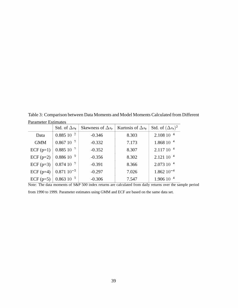
Table 3: Comparison between Data Moments and Model Moments Calculated from Different
Parameter EstimatesStd. of {r � Skewness of {r � Kurtosis of {r � Std. of E{r � � e
Data 0.885 �fl�e -0.346 8.303 2.108 �f
l �
GMM 0.867 �fl�e -0.332 7.173 1.868 �f
l �
ECF (p=1) 0.885 �fl�e -0.352 8.307 2.117 �f
l �
ECF (p=2) 0.886 �fl�e -0.356 8.302 2.121 �f
l �
ECF (p=3) 0.874 �fl�e -0.391 8.366 2.073 �f
l �
ECF (p=4) 0.871 �fl�e -0.297 7.026 1.862 �f
l �
ECF (p=5) 0.863 �fl�e -0.306 7.547 1.906 �f
l �Note: The data moments of S&P 500 index returns are calculated from daily returns over the sample period
from 1990 to 1999. Parameter estimates using GMM and ECF are based on the same data set.
39
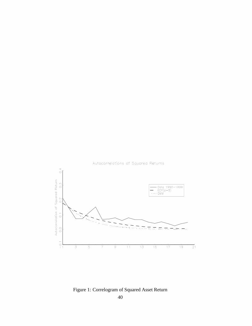
Figure 1: Correlogram of Squared Asset Return
40