Estimation and Impacts of Model Parameter1

Correlation for Seismic Performance Assessment of2

Reinforced Concrete Structures3

B.U. Gokkayaa,⇤, J.W. Bakera, G.G. Deierleina4

aCivil & Environmental Engineering Department and John A. Blume Earthquake5

Engineering Center, Stanford University, Stanford, CA 943056

Abstract7

Consideration of uncertainties, including stochastic dependence among8

uncertain parameters, is known to be important for estimating seismic risk9

of structures. In this study, we characterize the dependence of modeling10

parameters that define the nonlinear response at a component level and the11

interactions of multiple components associated with a system’s response. We12

utilize random e↵ects regression models, and a component test database with13

multiple tests conducted by di↵ering research groups, to estimate correlations14

among parameters. Groups of tests that are conducted in similar conditions,15

and are investigating the impacts of particular properties of components that16

can e↵ectively represent di↵erent locations in a structure, are suitable for this17

estimation approach. Correlation coe�cients from these regression models,18

reflecting statistical dependency among properties of components tested by19

individual research groups, are assumed here to reflect correlations associ-20

ated with multiple components in a structure. To illustrate, correlations for21

reinforced concrete element parameters are estimated from a database of re-22

inforced concrete beam-column tests, and then used to assess the e↵ects of23

⇤Corresponding author

Email addresses: beliz@alumni.stanford.edu (B.U. Gokkaya),

bakerjw@stanford.edu (J.W. Baker), ggd@stanford.edu (G.G. Deierlein)

Preprint submitted to Structural Safety March 22, 2017

correlations on dynamic response of a frame structure. Increased correla-24

tions are seen to increase dispersion in dynamic response and produce higher25

estimated probabilities of collapse. This work provides guidance for charac-26

terization of parameter correlations when propagating uncertainty in seismic27

response assessment of structures.28

Keywords: correlation, modeling uncertainty, random e↵ects regression,29

uncertainty propagation, collapse30

1. Introduction31

Performance-based earthquake engineering enables quantification and prop-32

agation of uncertainties in a probabilistic framework to make robust estima-33

tions of seismic risk and loss of structures. Quantification and propagation34

of ground motion uncertainties have received significant attention in the re-35

search community, but an important and somewhat less-explored topic is36

uncertainty in structural modeling (e.g., Bradley, 2013). The uncertainties37

related to use of idealized models and analysis methods, as well as uncertain-38

ties in a model’s parameters, influence assessments of the seismic reliability39

of a structure. Explicit quantification of uncertainties and characterization40

of dependence among the random model parameters are essential for propa-41

gating these uncertainties when assessing seismic performance.42

While quantification of model parameter uncertainties is relatively well43

studied, stochastic dependence among model parameters has received very44

little attention, in large part due to scarcity of appropriate calibration data.45

When it has been assessed or considered in assessments, it is typically in46

the form of correlation coe�cients. Where the random variables have a47

2

multivariate normal distribution, correlations provide a complete description48

of their dependence. They are also useful in first-order and other approximate49

reliability assessments.50

The current state-of-the-art in seismic reliability analysis is to use ex-51

pert judgment in quantifying the correlation structure of analysis model52

parameters. Haselton (2006) used judgment-based correlation coe�cients53

when considering model parameter uncertainty in assessing collapse risk of54

reinforced concrete structures, and showed that variability in collapse ca-55

pacity was strongly influenced by the correlation assumptions. Liel et al.56

(2009), Celarec and Dolsek (2013), Celik and Ellingwood (2010) and Pinto57

and Franchin (2014) all used assumed correlations among modeling parame-58

ters when propagating modeling uncertainty for seismic performance assess-59

ment of reinforced concrete structures.60

Although the e↵ects of correlations among random variables on system61

reliability are well known, few researchers have used observational data to62

quantify dependence. Idota et al. (2009) assessed the correlation of strength63

parameters for steel moment resisting frames using steel coupon tests from64

production lots. Vamvatsikos (2014) used those results to study the e↵ects of65

correlation of components at di↵erent locations in a building on its dynamic66

response. We are aware of no other studies that directly estimate correlations67

in component-level or phenomenological modeling parameters in order to68

study seismic collapse risk.69

In this study, we estimate the correlation structure of modeling param-70

eters that define a component’s nonlinear cyclic response, and study the71

interaction of di↵erent components on system-level dynamic response. Ran-72

3

dom e↵ects regression is used with a database of reinforced concrete column73

tests to infer correlation structure of parameters defining a concentrated plas-74

ticity model. The database is composed of reinforced concrete column tests75

performed by multiple research groups. Correlation coe�cients, representing76

statistical dependency among parameters within a set of tests conducted by a77

research group, are assumed to reflect dependency among parameters corre-78

sponding to components throughout a structural system. We then use the es-79

timated correlations to assess the e↵ects of correlations on dynamic response80

of a four-story reinforced concrete frame building, and to explore potential81

simplified approaches for representing parameter correlations. Although the82

reported correlation results are for reinforced concrete model parameters, the83

presented framework can be applied for other types of materials or models.84

2. Probabilistic Seismic Performance Assessment85

We use the probabilistic performance-based earthquake engineering method-86

ology to assess structural performance (e.g., Krawinkler and Miranda, 2004;87

Deierlein, 2004). Nonlinear structural analyses are run using a suite of ground88

motions to propagate uncertainties related to ground motion variability and89

seismic hazard. The results from structural analyses are then related to the90

risk of collapse and other damage states of interest.91

The concentrated plasticity model by Ibarra et al. (2005), which has92

been frequently used to simulate sidesway collapse in frame structures (e.g.,93

Zareian and Krawinkler, 2007; Eads et al., 2013), is used in this study to94

model component response. Specific attention is given to the correlation of95

model parameters used to define plastic hinges in seismic resisting moment96

4

frames. Phenomenological concentrated plasticity models are well-suited for97

modeling collapse of structures (Deierlein et al., 2010). However, model pa-98

rameters that define concentrated plasticity models are generally related to99

physical engineering parameters by empirical relationships. Modeling uncer-100

tainty becomes more pronounced for collapse response simulations than for101

elastic or mildly nonlinear simulations, due to both the relatively limited102

knowledge of parameter values and the highly nonlinear behavior associated103

with collapse.104

The concentrated plasticity model has a trilinear ”backbone curve,” shown105

in Figure 1, defined by five parameters: capping plastic rotation (✓cap,pl), ef-106

fective sti↵ness (secant sti↵ness up to 40% of the component yield moment107

EIstf ), yield moment (My), capping moment (Mc), and post-capping rota-108

tion (✓pc). A sixth parameter, �, defines the normalized energy dissipation109

capacity, which controls the rate of deterioration (under cyclic loading) of110

basic strength, post-capping strength, unloading sti↵ness, and accelerated111

reloading sti↵ness.112

The uncertainty in these modeling parameters is large, as estimated by113

a predictive model for these parameter values that will be discussed further114

below (Haselton et al., 2008). For a given column design, the parameters115

associated with elastic and peak strengths are moderately uncertain: the116

EIstf/EIg, My and Mc/My parameters have logarithmic standard deviations117

of 0.28, 0.3 and 0.1, respectively. The parameters associated with more non-118

linear displacement capacities and cyclic deterioration, however, are highly119

uncertain: the ✓pc, ✓cap,pl and � parameters have logarithmic standard devi-120

ations of 0.73, 0.59 and 0.51, respectively.121

5

My

Mc

Chord Rotation

Mo

me

nt

θpc

θcap,pl

EIstf

Figure 1: Ibarra et al. (2005) model for moment versus rotation of a plastic hinge

in a structure. The model parameters of interest are labeled.

In this study, we aim to characterize correlation of these model pa-122

rameters in a structure. Parameter correlations are grouped into within-123

component and between-component correlations. The former refers to cor-124

relations among modeling parameters that define response of a single com-125

ponent, whereas the latter refers to correlations among parameters from dif-126

fering components, as illustrated Figure 2. This distinction is useful because127

within-component correlations can be estimated from tests of individual com-128

ponents, while between-component correlations require more e↵ort to esti-129

mate. Between-component correlations are caused by similarities throughout130

a structure in the properties of structural materials, and member geometries131

and details. If these similarities are not captured in estimating mean val-132

ues for model parameters, they will result in stochastic dependence of the133

resulting component model parameters.134

Incremental dynamic analyses (IDA) involves performing nonlinear dy-135

6

Component i: { θcap,pl , My , ... }

Component j: { θcap,pl , My , ... }

Within-component

Between-component

Figure 2: Illustration of correlation within a component and correlation between

components in a structure.

namic analysis using multiple ground motions scaled to particular ground136

motion intensity measure (IM) levels (Vamvatsikos and Cornell, 2002). Seis-137

mic capacity is the IM value causing dynamic instability in the structure.138

This capacity is random due to the uncertain nature of a ground motion with139

a given IM level and uncertainties associated with structural performance.140

Its distribution is quantified by a collapse fragility function defining the prob-141

ability of collapse (C) at a given IM level, im (P (C|IM = im)). Below, the142

fragility function will be estimated either by an empirical distribution or by143

7

fitting a lognormal cumulative distribution function:144

P (C|IM = im) = �

✓ln (im/✓)

�

◆(1)

where � () is a standard normal cumulative distribution function, ✓ is the145

median and � is the logarithmic standard deviation (or “dispersion”) of the146

distribution. Values for ✓ and � will be estimated and reported below.147

The mean annual frequency of collapse (�c) is obtained by integrating a148

collapse fragility function with a ground motion hazard curve (Ibarra and149

Krawinkler, 2005), as given in Equation 2.150

�c =

Z 1

0

P (C|IM = im)

����d�IM(im)

d(im)

���� d(im) (2)

where �IM(im) is the mean annual rate of exceeding the ground motion im151

and d�IM (im)d(im)

defines the slope of the hazard curve at im.152

Fragility functions corresponding to alternative limit states, such as ex-153

ceeding a particular story drift ratio, sdr, can be also obtained from incre-154

mental dynamic analysis results. Using IDA, ground motions are scaled until155

the structure displays a story drift ratio of sdr and the fragility function is156

obtained. This function can be integrated with the seismic hazard curve157

in a similar fashion to Equation 2 to estimate the mean annual frequency158

(�SDR�sdr) of exceeding a given limit state.159

3. Assessing Correlations of Model Parameters160

The correlation assessment procedure described in this section requires161

two inputs: (1) a set of observed parameter values from test data where there162

are groups of components analogous to a set of components in a building,163

8

and (2) predictive equations that estimate means and standard deviations of164

those parameters values based on component properties such as dimensions165

and material strengths. With those two inputs, a mixed e↵ects analysis166

can be performed to estimate correlations as described here. It would also167

be natural to start with only the observed parameter values, and fit the168

predictive equations at the same time as the correlations are estimated. To169

illustrate, we consider the case of concrete beam-columns with the lumped-170

plasticity component model described above; in this case predictive equations171

for means and standard deviations are already available, so we adopt those172

equations and focus only on the estimation of correlations.173

3.1. Observed Parameter Values174

The six parameters illustrated in Figure 1 are treated here as random175

variables. Haselton et al. (2008) estimated values for these parameters for176

255 column tests from the Pacific Earthquake Engineering Research Center177

Structural Performance Database (Berry et al., 2004). This database pro-178

vides force-displacement histories from cyclic and lateral-load tests, along179

with information related to reinforcement, column geometry, test configura-180

tion, axial load, and failure type for each column.181

Haselton et al. (2008) considered rectangular column tests whose failure182

modes were either flexure or combined flexure and shear. The model param-183

eters were calibrated so that a cantilever column, with an elastic element184

and a concentrated plastic hinge at the base, has behavior that matches the185

corresponding experimental force-displacement data. The study authors fil-186

tered the data to remove outliers and parameters whose values could not187

be estimated for a given test (typically these were parameters characteriz-188

9

ing post-peak cyclic deterioration response, in cases where a test did not189

induce this behavior). The total number of estimated parameter values are190

232, 197, 255, 233, 65 and 223 for ✓cap,pl, EIstf/EIg, My, Mc/My, ✓pc and �,191

respectively.192

The 255 column tests used for the calibration were conducted by 42 di↵er-193

ent research laboratories, referred to here as “test groups”. The test groups194

are listed in Table 6, along with information for each regarding the varia-195

tion among tests in member dimensions, concrete strength (f 0c), longitudinal196

yield strength (fy), axial load ratio, and area of longitudinal and transverse197

reinforcement.198

3.2. Evidence of Parameter Correlations199

Using the observed parameter values described above, we compute pre-200

diction residuals by comparing the observations to model predictions:201

ln�y

kij

�= ln

�y

kij

�+ "

kij (3)

where subscripts i and j represent the test group and test number, respec-202

tively, and the superscript k indicates the random variable of interest. Ran-203

dom variable k from the test specified by i and j is associated with observed204

value y

kij, predicted value y

kij, and residual "kij.205

Predicted values are obtained in this study from the empirical equations of206

Haselton et al. (2008) and Panagiotakos and Fardis (2001). These equations207

relate column design details to the six model parameters using equations that208

are based on regression analysis of observed data and judgment on expected209

behavior. Haselton et al. (2008) provide a full and a simplified equation for210

10

some of the model parameters; we use the full equations if both are provided.211

The predictive model studies found that parameter values are generally log-212

normal, so a logarithmic transformation is used in equation 3 (and in the213

original predictive models) to obtain normally distributed residuals.214

For each model parameter, the residuals from each group of tests are215

plotted against each other, and a subset of the data are shown for illustra-216

tion in Figure 3. Each test group is denoted by a specific symbol and color.217

Grouping of these residuals by test group implies the presence of correlated218

residuals; this is most evident for My in Figure 3c. Here it is observed that219

tests from group 1 (TG1) have negative residuals, implying that the My val-220

ues of the tests conducted in that test group are consistently overestimated221

by the predictive equation. Conversely, tests from group 3 (TG3) have posi-222

tive residuals indicating an underestimation of observations by the predictive223

equation.224

The grouping of residuals within test groups is not surprising, considering225

that the tests have common features whose e↵ects are not captured by the226

predictive equations. Reviewing Table 6 in the Appendix, we observe that: 1)227

The majority of groups have tests with similar specimen dimensions. 2) Steel228

yield strength and area ratio of longitudinal reinforcing steel are constant in229

approximately three-quarters of the test groups. 3) The major di↵erences230

among the tests within each group are the level of axial load and transverse231

reinforcement. While not explicitly documented, we also expect that tests232

from a single laboratory would have similarities in environmental conditions,233

workmanship, and other factors that might influence the component behav-234

ior. These features within each test group are similar to features we would235

11

−1 0 1

−1

0

1

ε k

εk

θcap,pl

(a)

−0.5 0 0.5

−0.6

0

0.6

ε k

εk

EIstf/EI

g

(b)

−1 0 1

−1

0

1

ε k

εk

My

(c)

TG1

TG3

Figure 3: Example model parameter residuals, ("k), plotted against the residuals

of other tests within the test group to which they belong for a) ✓cap,pl, b) EIstf/EIg,

c) My. A subset of data is shown for illustrative purposes.

expect to see among components located throughout a real-world building.236

When modeling seismic performance of a real structure, we would use the237

same predictive equations discussed above to predict parameter values for a238

numerical model. Because those predictive models rely on the limited set of239

column properties, we would expect components in a real building to also240

behave in a correlated (but not perfectly dependent) manner. By assuming241

that a group of components in a single laboratory’s tests corresponds to a242

group of components in a building, we can utilize statistical analysis of this243

test data to quantitatively estimate parameter correlations for components244

within a real building. While the correspondence between test groups and245

real-world structures is not strictly true, the authors believe it is reasonable,246

and this assumption provides a unique opportunity to estimate correlations247

that are otherwise nearly impossible to observe. We will keep in mind the248

12

approximate nature of this correspondence when evaluating the numerical249

results below.250

3.3. Random E↵ects Regression251

The observed clustering of residuals within a test group motivates the252

use of random e↵ects regression to study the correlations among model pa-253

rameters. Random e↵ects models are used when at least one of the response254

variables is categorical. The discrete levels for the categorical variable are255

termed the “e↵ects” in the model, and the qualifier random implies that the256

observed levels represent a random sample from a population and do not257

contain all possible levels (Searle et al., 2009; Pinheiro and Bates, 2010).258

A one-way random e↵ects model is applied to residuals from Equation259

3 to assess the correlation structure of the model parameters, using the R260

software package (Team, 2014). The test groups are treated as a random261

e↵ect, and logarithmic residuals of each random variable, "kij, are considered262

without any further transformation, leading to the following equation:263

ln�y

kij

�� ln

�y

kij

�= "

kij

= µ

k + ↵

ki + "

kij

(4)

where where µ

k is an intercept indicating the mean of the data, and ↵

k and264

"

k represent between- and within-test-group variability, respectively. The265

↵

k and "

k terms are independent random variables with zero means and266

variances �

2k and ⌧

2k , respectively. These variances are estimated from the267

regression procedure. From Equation 4 and the above definitions, it follows268

that the variance of a model parameter, k, is �2k + ⌧

2k .269

13

From Equation 4, the covariance of the logarithms of the model parame-270

ters k and k

0 within a component j is given by:271

cov

⇣ln�y

kij

�, ln

⇣y

k0

ij

⌘⌘= cov("kij, "

k0

ij )

= cov(µk + ↵

ki + "

kij, µ

k0 + ↵

k0

i + "

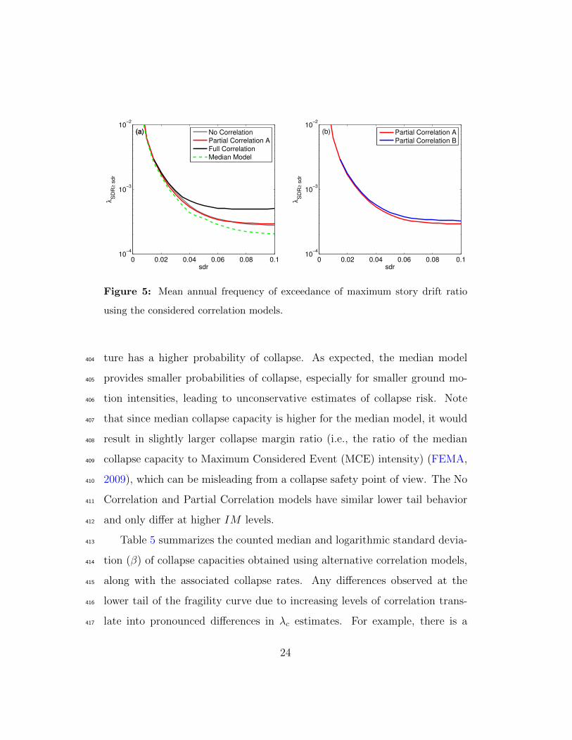
k0

ij )

= corr(↵ki ,↵

k0

i )�k�k0 + corr("kij, "k0

ij )⌧k⌧k0

(5)

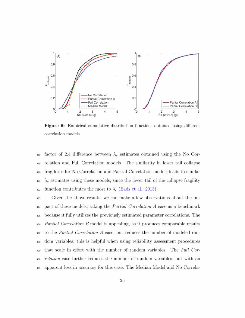
where cov(·, ·) and corr(·, ·) refer to covariance and correlation, and by def-272

inition cov(↵ki ,↵

k0j ) = corr(↵k

i ,↵k0i )�k�k0 and cov("ki , "

k0j ) = corr("ki , "

k0i )⌧k⌧k0 .273

Correlation of model parameters within a component is then given by:274

corr(ln�y

kij

�, ln

⇣y

k0

ij

⌘) =

corr

�↵

ki ,↵

k0i

��k�k0 + corr

�"

kij, "

k0ij

�⌧k⌧k0p

�

2k + ⌧

2k

p�

2k0 + ⌧

2k0

(6)

The covariance of the logarithms of the model parameters k and k

0 between275

components j and j

0 is given by:276

cov(ln�y

kij

�, ln

⇣y

k0

ij0

⌘) = cov(µk+↵

ki +"

kij, µ

k0+↵

k0

i +"

k0

ij0) = corr(↵ki ,↵

k0

i )�k�k0

(7)

where the cov("kij, "k0ij0) = 0 since "

kij and "

k0ij0 are independent. Correlation of277

model parameters between components can then be shown to equal278

corr(ln�y

kij

�, ln

⇣y

k0

ij0

⌘) =

corr

�↵

ki ,↵

k0i

��k�k0p

�

2k + ⌧

2k

p�

2k0 + ⌧

2k0

(8)

When assessing the correlation of the same model parameter between279

components, corr(↵ki ,↵

ki ) = 1 and Equation 8 simplifies to280

corr(ln�y

kij

�, ln

�y

kij0�) =

�

2k

�

2k + ⌧

2k

(9)

14

Table 1: Between and within test group standard deviations obtained from ran-

dom e↵ects regression.

�k ⌧k

p�

2k + ⌧

2k

✓cap,pl 0.41 0.44 0.59EIstfEIg

0.20 0.20 0.28

My 0.26 0.10 0.30

McMy

0.07 0.08 0.10

✓pc 0.24 0.69 0.73

� 0.20 0.46 0.51

3.4. Regression Results281

Estimated between-component (�k) and within-component (⌧k) standard282

deviations for the example database are shown in Table 1. Table 2 shows283

the correlation coe�cients obtained using Equations 5 to 9. Table 3 shows284

the same correlation coe�cients obtained after rounding to one significant285

figure, reflecting the approximate nature of the way in which we are using286

these data and the finite sized database used here. The correlations shown287

in Table 3 are used in the rest of the paper.288

15

Table

2:Initialcorrelationcoe�cientsobtainedfrom

random

e↵ectsregression.

Componenti

Componentj

✓ cap,pl i

⇣EI s

tf

EI g

⌘ iM

yi

⇣M

cM

y

⌘ i✓ p

c i� i

✓ cap,pl j

⇣EI s

tf

EI g

⌘ jM

yj

⇣M

cM

y

⌘ j✓ p

c j� j

Componenti

✓ cap,pl i

1.0000

-0.0183

0.0578

0.2538

0.2083

-0.0260

0.6839

0.0106

0.0277

0.0975

0.0533

-0.0202

⇣EI s

tf

EI g

⌘ i1.0000

0.1354

-0.1018

0.0375

0.0799

0.6853

0.0612

-0.0950

-0.0305

0.0379

Myi

1.0000

0.2838

0.1067

0.0722

0.9263

0.2482

0.0951

0.0549

⇣M

cM

y

⌘ j1.0000

0.0077

0.1681

0.6728

0.0415

0.0192

✓ pc i

(sym.)

1.0000

0.2195

(sym.)

0.3466

0.0357

� i1.000

0.4102

16

Table

3:Finalcorrelationcoe�cientsareobtainedafterroundingtoonesignificantfigure.

Com

pon

enti

Com

pon

entj

✓

cap,pl i

⇣EI s

tf

EI g

⌘ iM

y i

⇣M

cM

y

⌘ i✓

pc i

�

i✓

cap,pl j

⇣EI s

tf

EI g

⌘ jM

y j

⇣M

cM

y

⌘ j✓

pc j

�

j

Componenti

✓

cap,pl i

1.0

0.0

0.1

0.3

0.2

0.0

0.7

0.0

0.0

0.1

0.1

0.0

⇣EI s

tf

EI g

⌘ i1.0

0.1

-0.1

0.0

0.1

0.7

0.1

-0.1

0.0

0.0

M

y i1.0

0.3

0.1

0.1

0.9

0.2

0.1

0.1

⇣M

cM

y

⌘ j1.0

0.0

0.2

0.7

0.0

0.0

✓

pc i

(sym

.)1.0

0.2

(sym

.)0.3

0.0

�

i1.0

0.4

17

We note that rounding of the correlation coe�cients, and estimation of289

correlations from data with missing values, can result in a correlation matrix290

without the required positive semi-definiteness property. Although Table 3291

produces positive definite matrices, in our initial calculations some violation292

of positive semi-definiteness was observed. In such cases, minor changes293

can be made to transform the correlation matrix into a positive definite one294

(Jackel, 2001).295

We observe that within a component (i.e., the left half of Table 3), corre-296

lations of model parameters are rather small; the largest coe�cient being 0.3,297

which corresponds to the correlations between Mc/My and My, and Mc/My298

and ✓cap,pl. These values suggest moderate interactions between strength pa-299

rameters and hardening behavior. Small interactions are observed between300

the parameters defining post-capping cyclic behavior within a component301

(e.g., � with Mc/My and ✓pc).302

Between components, like parameters have larger correlation coe�cients303

(i.e., the diagonal components on the right half of Table 3). We see that My,304

✓cap,pl, EIstf/EIg and Mc/My have correlations of 0.7 or greater. In the set-305

ting of a structure, this implies that values of these parameters across compo-306

nents will tend to take similar values; note that Haselton and Deierlein (2007)307

and Liel et al. (2009) assumed perfect correlation between like-parameters308

across components.309

We also observe that correlations of di↵erent model parameters between310

components are small (i.e., the o↵-diagonal terms in the right half of the311

table). This is expected, given that the correlations of these parameters312

within a component are also small. There is even a small negative correlation313

18

between EIstf/EIg and Mc/My. This is likely to be a numerical artifact, as314

there is no clear physical reason why such a correlation would be negative.315

This artifact also motivates the decision to retain only one significant figure316

in the correlation estimates.317

4. Impacts of Parameter Correlations on Dynamic Structural Re-318

sponse319

4.1. Case Study Structure320

A reinforced concrete special moment frame structure is considered here,321

to demonstrate the impact of parameter correlations and evaluate potential322

model simplifications for structures with many uncertain parameters. The323

building was designed by Haselton (2006) for a high seismicity site in Cali-324

fornia in accordance with 2003 IBC and ASCE 7-02 provisions (IBC, 2003;325

American Society of Civil Engineers, 2002). Here we assume the building to326

be located at the same Los Angeles site as considered in its original design.327

One three-bay four-story frame of the building is modeled, with a total of328

12 beam and 16 column elements. The structural system is modeled using329

the concentrated plasticity approach described above, in which elements of330

the frame are modeled using elastic elements with rotational springs at the331

ends. A Rayleigh damping of 3% is defined at the first and third mode pe-332

riods of the structure, and P-� e↵ects are modeled using a leaning column.333

The fundamental period of the structure is 0.94 s. The Open System for334

Earthquake Engineering Simulation platform is used to analyze the struc-335

ture (OpenSEES, 2015). The FEMA-P695 far-field set of 44 ground motion336

components is used for structural response simulations (FEMA, 2009).337

19

Monte Carlo simulation is used for propagating uncertainties related to338

modeling and ground motion variability (Kalos and Whitlock, 2009). The339

six parameters mentioned previously are treated as random, with marginal340

means and standard deviations as predicted by Haselton et al. (2008), and341

correlations as defined below. Further, equivalent viscous damping and col-342

umn footing rotational sti↵ness are assumed to be random, with logarithmic343

standard deviation values of 0.6 and 0.3, respectively (Haselton, 2006; Hart344

and Vasudevan, 1975; Porter et al., 2002), and to be independent of the345

other parameters. A multivariate normal distribution is assumed for the346

logarithms of all parameters except Mc/My. Since, by definition Mc/My is347

always greater than 1, we use a one-sided truncated normal distribution for348

this parameter. Because only one frame of the structure is modeled, it is349

implicitly assumed that the parameters for frames in a given direction are350

fully correlated.351

Table 4 lists four correlation models considered in the following analyses.352

As the name implies, the No Correlation model assumes all parameters in353

the building to be uncorrelated. This model has 170 random variables (six354

parameters for each of 28 elements, plus damping and foundation sti↵ness355

parameters). The Partial Correlation A model uses correlation coe�cients356

from Table 3 for all within- and between-component correlations, and also357

has 170 random variables. In Partial Correlation B, Table 3 is used to define358

correlations within a component and correlations of beam-to-column com-359

ponents. Column-to-column and beam-to-beam parameters are assumed to360

be fully correlated (e.g., all column components for a given model realiza-361

tion have the same parameters). These assumed full correlations reduce the362

20

Table 4: Correlation models used with Monte Carlo simulations. “0”, “P” and “1”

refer to the cases of No Correlation, Partial Correlation and Perfect Correlation,

respectively.

Within- Between-component E↵ective

Model Name component Column-

to-Column

Beam-to-

Beam

Beam-to-

Column

# of

R.V.s

No Correlation 0 0 0 0 170

Partial Correlation A P P P P 170

Partial Correlation B P 1 1 P 16

Full Correlation 1 1 1 1 3

e↵ective number of random variables for this model to 14 (six beam param-363

eters, six column parameters, damping and foundation sti↵ness). In the Full364

Correlation model all of the element parameters are assumed to have per-365

fect correlation, such that there are e↵ectively three random variables (one366

component parameter, damping and foundation sti↵ness).367

For each correlation model, we simulate 4400 realizations of model pa-368

rameters from their joint distribution, each of which are randomly matched369

with one ground motion. Incremental dynamic analysis is then conducted370

to scale each ground motion up until structural collapse is observed for the371

given model realization. A maximum story drift ratio (SDR) � 0.1 is as-372

sumed to indicate structural collapse. Ground motion IM values are defined373

as 5%-damped first-mode spectral acceleration, Sa(0.94s).374

21

0 0.02 0.04 0.06 0.08 0.10

0.5

1

1.5

2

SDR

Me

dia

n S

a (

0.9

4 s

) (g

)

(a)(a)(a)(a)

No CorrelationPartial Correlation AFull CorrelationMedian Model

0 0.02 0.04 0.06 0.08 0.10

0.5

1

1.5

2

SDR

(b)(b)(b)

Partial Correlation APartial Correlation B

0 0.02 0.04 0.06 0.08 0.10

0.1

0.2

0.3

0.4

0.5

0.6

SDR

Dis

pe

rsio

n

Me

dia

n S

a (

0.9

4 s

) (g

)D

isp

ers

ion

(c)(c)

No CorrelationPartial Correlation AFull CorrelationMedian Model

0 0.02 0.04 0.06 0.08 0.10

0.1

0.2

0.3

0.4

0.5

0.6

SDR

(d)

Partial Correlation APartial Correlation B

Figure 4: IDA results obtained using di↵erent correlation models a) median

IDA response for varying correlation levels, b) median IDA response for Partial

Correlation models, c) dispersion in IDA curves for varying correlation levels, and

d) dispersion in IDA curves for Partial Correlation models.

4.2. Results375

Figures 4.a and 4.b show the median IDA curves from the four correlation376

models, along with results for a structure with median model parameters (i.e.,377

no parameter uncertainty). There are remarkably small di↵erences among378

22

the median IDA curves. A small di↵erence between the No Correlation and379

Full Correlation cases is observed for SDR � 0.03, with a di↵erence of 7%380

at SDR = 0.1.381

Figures 4.c and 4.d show the dispersions in the IDA curves, and these vary382

more significantly. The Partial Correlation A and No Correlation models383

yield similar variability for SDR< 0.03, and at SDR= 0.1, the di↵erence in384

dispersion values for these two cases is 12%. At SDR= 0.1, the di↵erence in385

dispersion between No Correlation and Full Correlation models is 47%. The386

Median model consistently underestimates dispersion, where for SDR= 0.1,387

a di↵erence of 17% is observed between dispersion values of Median and388

Partial Correlation models. The Partial Correlation A and B models have389

very similar medians and dispersions.390

The mean annual frequency of collapse, �c, is obtained by integrating391

the empirical collapse fragility curves with the seismic hazard curve of the392

Los Angeles site using equation 2. Fragility functions and corresponding and393

�SDR�sdr values are also obtained for alternative values of sdr. Figure 5394

shows �SDR�sdr with respect to sdr using the assumed correlation models,395

where the �SDR�sdr di↵er for SDR values greater than approximately 0.03.396

The plots show, for example, that the No Correlation and Partial Correlation397

cases produce nearly identical �SDR�sdr. On the other hand, the �SDR�sdr398

for the Full Correlation case is 30% to 110% higher than the No Correlation399

model for drift values of 0.05 and 0.1, respectively.400

Figure 6 shows empirical collapse cumulative distribution functions for401

the structure obtained using the considered correlation models. At smaller402

Sa(0.94s)) levels, as the correlations among parameters increase, the struc-403

23

0 0.02 0.04 0.06 0.08 0.110

−4

10−3

10−2

sdr

λS

DR

≥ s

dr

(a)(a) No CorrelationPartial Correlation AFull CorrelationMedian Model

0 0.02 0.04 0.06 0.08 0.110

−4

10−3

10−2

sdr

λS

DR

≥ s

dr

(b) Partial Correlation APartial Correlation B

Figure 5: Mean annual frequency of exceedance of maximum story drift ratio

using the considered correlation models.

ture has a higher probability of collapse. As expected, the median model404

provides smaller probabilities of collapse, especially for smaller ground mo-405

tion intensities, leading to unconservative estimates of collapse risk. Note406

that since median collapse capacity is higher for the median model, it would407

result in slightly larger collapse margin ratio (i.e., the ratio of the median408

collapse capacity to Maximum Considered Event (MCE) intensity) (FEMA,409

2009), which can be misleading from a collapse safety point of view. The No410

Correlation and Partial Correlation models have similar lower tail behavior411

and only di↵er at higher IM levels.412

Table 5 summarizes the counted median and logarithmic standard devia-413

tion (�) of collapse capacities obtained using alternative correlation models,414

along with the associated collapse rates. Any di↵erences observed at the415

lower tail of the fragility curve due to increasing levels of correlation trans-416

late into pronounced di↵erences in �c estimates. For example, there is a417

24

0 1 2 3 4 50

0.2

0.4

0.6

0.8

1

Pco

llap

se

(a)(a)

No CorrelationPartial Correlation AFull CorrelationMedian Model

0 1 2 3 4 50

0.2

0.4

0.6

0.8

1

Sa (0.94 s) (g)Sa (0.94 s) (g)

Pco

llap

se

(b)

Partial Correlation APartial Correlation B

Figure 6: Empirical cumulative distribution functions obtained using di↵erent

correlation models

factor of 2.4 di↵erence between �c estimates obtained using the No Cor-418

relation and Full Correlation models. The similarity in lower tail collapse419

fragilities for No Correlation and Partial Correlation models leads to similar420

�c estimates using these models, since the lower tail of the collapse fragility421

function contributes the most to �c (Eads et al., 2013).422

Given the above results, we can make a few observations about the im-423

pact of these models, taking the Partial Correlation A case as a benchmark424

because it fully utilizes the previously estimated parameter correlations. The425

Partial Correlation B model is appealing, as it produces comparable results426

to the Partial Correlation A case, but reduces the number of modeled ran-427

dom variables; this is helpful when using reliability assessment procedures428

that scale in e↵ort with the number of random variables. The Full Cor-429

relation case further reduces the number of random variables, but with an430

apparent loss in accuracy for this case. The Median Model and No Correla-431

25

Table 5: Counted median and logarithmic standard deviation (�ln) of collapse

capacity, and mean annual frequency of collapse (�c), obtained using alternative

models.

Model Name Median � �c (⇤10�4)

Median Model 1.69 0.39 1.81

No Correlation 1.57 0.42 2.65

Partial Correlation A 1.67 0.48 2.75

Partial Correlation B 1.64 0.49 3.06

Full Correlation 1.69 0.67 6.39

tions cases are also simplified representations of the model, but they produce432

unconservative estimates of seismic collapse risk and so should be used with433

caution.434

The structure considered here was designed to have a regular strength and435

sti↵ness distribution over its height, and so the typical collapse mechanisms436

were not notably altered when considering No Correlation and Partial Corre-437

lation models. Although we did not investigate the influence of ductility and438

strength irregularities in detail, we expect that di↵erent results are likely to439

be obtained for buildings with strength irregularities, since presence of even440

partial correlations may enable the triggering of alternate modes of failure441

(e.g., creation of a story mechanism by simulation of weak column-strength442

parameters).443

26

5. Conclusions444

We have considered model parameter uncertainty in seismic performance445

assessment of structures, both in estimating parameter correlations and in446

quantifying the impacts of these correlations on building performance. We447

have characterized the dependence of modeling parameters that define cyclic448

inelastic response at a component level and the interactions of multiple com-449

ponents associated with a system’s response. Parameter correlations were450

estimated from component tests using random e↵ects regression on grouped451

tests of structural components. Variation in parameter values within and452

between test groups were incorporated as random e↵ects in the regression453

model, and statistical dependency between the estimated parameters were454

assessed.455

Dependence in the parameters defining a lumped-plasticity model for con-456

crete columns were estimated using a database of reinforced concrete beam-457

column tests. Correlation coe�cients from these regression models, reflecting458

statistical dependency among properties of components tested by individ-459

ual research groups, are assumed to reflect correlations among components460

within a given structure. The random treatment of research groups, com-461

bined with the aforementioned observations in the data set (i.e., similarity of462

column dimensions and di↵erences in axial load and transverse reinforcement463

in the tests), justified this assumption. We found that correlations between464

di↵ering parameters (both within and between components) have low corre-465

lation (correlation coe�cients from -0.1 to 0.3), while like parameters across466

components have higher correlations of as large as 0.9.467

The impact of these estimated parameter correlations on dynamic re-468

27

sponse of a four story reinforced concrete frame structure was then assessed,469

by performing Incremental Dynamic Analysis of the structure using Monte470

Carlo realizations of uncertain model parameters. Variations in correlation471

assumptions did not strongly influence median response, even for large drifts.472

Variability in correlation assumptions did, however significantly influence dis-473

persion in response estimates, especially at large drift levels associated with474

severe nonlinearity and collapse. Models considering uncorrelated and par-475

tially correlated parameters had similar collapse fragility functions at the476

critical lower tail, resulting in similar mean annual frequencies of collapse.477

Models assuming perfectly correlated parameters, however, had higher prob-478

abilities of collapse for low-intensity shaking; the perfectly correlated model479

had a mean annual frequency of collapse that was 2.4 times the frequency480

of collapse of the fully uncorrelated model (even though the parameters had481

the same marginal distributions in both cases). A slightly simplified model482

representation, with full correlation among beam-to-beam and column-to-483

column parameters (and partially correlated beam-to-column parameters),484

produced nearly identical results to the benchmark model with partial corre-485

lations in all parameters. This simplified model has significantly fewer unique486

random variables, and so is a promising approach for considering parameter487

correlations while also managing computational expense. In aggregate, these488

results provide further evidence that parameter correlations are an important489

consideration in seismic collapse safety assessments.490

The results presented here were for reinforced concrete components, but491

the framework allows these evaluations to be performed on any model with492

uncertain parameters that are estimated from experimental data. The cor-493

28

relation estimation approach requires a set of component tests with multiple494

tests that can be grouped and considered as having commonalities consis-495

tent with those among components in a given structure. Tests that are496

conducted in similar conditions, and are investigating the impacts of partic-497

ular properties of components, are most suitable for this approach. While498

the appropriateness of considering groups of tests to represent components499

throughout a structure will need to be evaluated on a case-by-case basis, this500

proposed approach o↵ers a unique solution to the otherwise vexing problem501

of estimating parameter correlations for studying the seismic reliability of502

buildings.503

6. Data and Resources504

The data for the reinforced concrete column tests are obtained from the505

PEER Structural Performance Database (http://nisee.berkeley.edu/spd/)506

and Professor Curt Haselton’s Reinforced Concrete Element Calibration Database507

(http://www.csuchico.edu/structural/researchdatabases/reinforced_508

concrete_element_calibration_database.shtml).509

7. Acknowledgements510

We thank Dr. Shrey Shahi and Professor Art Owen for providing valu-511

able feedback on mixed e↵ects modeling. This work was supported by the512

National Science Foundation under NSF grant number CMMI-1031722. Any513

opinions, findings and conclusions or recommendations expressed in this ma-514

terial are those of the authors and do not necessarily reflect the views of the515

National Science Foundation.516

29

8. References517

American Society of Civil Engineers (2002). ASCE Standard 7-02: Minimum518

Design Loads for Buildings and Other Structures. Reston, VA.519

Amitsu, S., Shirai, N., Adachi, H., and Ono, A. (1991). Deformation of rein-520

forced concrete column with high or fluctuating axial force. Transactions521

of the Japan Concrete Institute, 13:35–362.522

Ang, B. G. (1981). Ductility of reinforced concrete bridge piers under seis-523

mic loading. Master’s thesis, University of Canterbury. Civil and Natural524

Resources Engineering.525

Arakawa, T., Arai, Y., Egashira, K., and Fujita, Y. (1982). E↵ects of the526

rate of cyclic loading on the load-carrying capacity and inelastic behavior of527

reinforced concrete columns. Transactions of the Japan Concrete Institute,528

4:485–492.529

Atalay, M. B. and Penzien, J. (1975). Behavior of critical regions of re-530

inforced concrete components as influenced by moment, shear and axial531

force. Earthquake Engineering Research Center, Report No. EERC 75, 19.532

Azizinamini, A., Johal, L. S., Hanson, N. W., Musser, D. W., and Corley,533

W. G. (1988). E↵ects of transverse reinforcement on seismic performance534

of columns: A partial parametric investigation. Technical report, Con-535

struction Technology Laboratories, Inc.536

Bayrak, O. and Sheikh, S. A. (1996). Confinement steel requirements for high537

strength concrete columns. In Proceedings of the 11th World Conference538

on Earthquake Engineering, number 463. Elsevier Science Ltd.539

30

Bayrak, O. and Sheikh, S. A. (2001). Plastic hinge analysis. Journal of540

Structural Engineering, 127(9):1092–1100.541

Bechtoula, H. (1985). Damage assessment of reinforced concrete columns un-542

der large axial and lateral loadings. Technical report, Dept. of Architecture543

and Architectural Systems, Kyoto University.544

Berry, M., Parrish, M., and Eberhard, M. (2004). PEER structural per-545

formance database users manual (version 1.0). University of California,546

Berkeley.547

Bradley, B. A. (2013). A critical examination of seismic response uncertainty548

analysis in earthquake engineering. Earthquake Engineering & Structural549

Dynamics, 42(11):1717–1729.550

Celarec, D. and Dolsek, M. (2013). The impact of modelling uncertainties on551

the seismic performance assessment of reinforced concrete frame buildings.552

Engineering Structures, 52:340–354.553

Celik, O. C. and Ellingwood, B. R. (2010). Seismic fragilities for non-ductile554

reinforced concrete frames Role of aleatoric and epistemic uncertainties.555

Structural Safety, 32(1):1–12.556

Deierlein, G. G. (2004). Overview of a comprehensive framework for earth-557

quake performance assessment. Technical report, International Work-558

shop on Performance-Based Seismic Design Concepts and Implementation,559

Bled, Slovenia.560

Deierlein, G. G., Reinhorn, A. M., and Willford, M. R. (2010). Nonlinear561

31

structural analysis for seismic design. NEHRP Seismic Design Technical562

Brief (NIST GCR 10-917-5), 4.563

Eads, L., Miranda, E., Krawinkler, H., and Lignos, D. G. (2013). An e�cient564

method for estimating the collapse risk of structures in seismic regions.565

Earthquake Engineering & Structural Dynamics, 42(1):25–41.566

Esaki, F. (1996). Reinforcing e↵ect of steel plate hoops on ductility of r/c567

square columns. In Proc., 11th World Conf. on Earthquake Engineering,568

page 199. Pergamon, Elsevier Science.569

FEMA (2009). Quantification of Building Seismic Performance Factors.570

FEMA-P695. Federal Emergency Management Agency.571

Galeota, D., Giammatteo, M. M., and Marino, R. (1996). Seismic resistance572

of high strength concrete columns. In Proceedings of the 11th World Con-573

ference on Earthquake Engineering, number 1383. Elsevier Science Ltd.574

Gill, W. D. (1979). Ductility of rectangular reinforced concrete columns with575

axial load. Technical report, University of Canterbury, Department of Civil576

Engineering, New Zealand.577

Hart, G. C. and Vasudevan, R. (1975). Earthquake Design of Build-578

ings:Damping. Journal of the Structural Division, 101(1):11–30.579

Haselton, C. (2006). Assessing Seismic Collapse Safety of Modern Reinforced580

Concrete Moment Frame Buildings. Dept. of Civil and Environmental581

Engineering. Stanford University, Stanford, CA.582

32

Haselton, C. B. and Deierlein, G. G. (2007). Assessing seismic collapse safety583

of modern reinforced concrete moment frame buildings. Technical Re-584

port Technical report, Report 2007/08, Pacific Earthquake Engineering585

Research Center, Berkeley, CA.586

Haselton, C. B., Liel, A. B., Lange, S. T., and Deierlein, G. G. (2008). Beam-587

column element model calibrated for predicting flexural response leading588

to global collapse of RC frame buildings. Technical Report PEER 2007/03,589

Pacific Earthquake Engineering Research Center, University of California590

at Berkeley, Berkeley, California.591

Ibarra, L. F. and Krawinkler, H. (2005). Global collapse of frame structures592

under seismic excitations. Technical report, John A. Blume Earthquake593

Engineering Center, Stanford, CA.594

Ibarra, L. F., Medina, R. A., and Krawinkler, H. (2005). Hysteretic models595

that incorporate strength and sti↵ness deterioration. Earthquake Engi-596

neering & Structural Dynamics, 34(12):1489–1511.597

IBC (2003). International Building Code. International Code Council (ISBN:598

1892395568).599

Idota, H., Guan, L., and Yamazaki, K. (2009). Statistical correlation of600

steel members for system reliability analysis. In Proceedings of the 9th601

International Conference on Structural Safety and Reliability (ICOSSAR),602

Osaka, Japan.603

Jackel, P. (2001). Monte Carlo methods in finance. Stochastic Dynamics,604

3:3–2.605

33

Kalos, M. H. and Whitlock, P. A. (2009). Monte Carlo Methods. John Wiley606

& Sons.607

Kanda, M., Shirai, N., Adachi, H., and Sato, T. (1988). Analytical study on608

elasto-plastic hysteretic behaviors of reinforced concrete members. Trans-609

actions of the Japan Concrete Institute, 10:257–264.610

Krawinkler, H. and Miranda, E. (2004). Performance-based earthquake611

engineering. Earthquake Engineering: From Engineering Seismology to612

Performance-Based Engineering (edited by Y. Bozorgnia and VV Bertero),613

CRC Press, Boca Raton, USA.614

Legeron, F. and Paultre, P. (2000). Behavior of high-strength concrete615

columns under cyclic flexure and constant axial load. ACI Structural Jour-616

nal, 97(4).617

Liel, A. B., Haselton, C. B., Deierlein, G. G., and Baker, J. W. (2009).618

Incorporating modeling uncertainties in the assessment of seismic collapse619

risk of buildings. Structural Safety, 31(2):197–211.620

Lynn, A. C. (2001). Seismic evaluation of existing reinforced concrete building621

columns. PhD thesis, University of California at Berkeley.622

Lynn, A. C., Moehle, J. P., Mahin, S. A., and Holmes, W. T. (1996). Seismic623

evaluation of existing reinforced concrete building columns. Earthquake624

Spectra, 12(4):715–739.625

Matamoros, A. B. (1999). Study of drift limits for high-strength concrete626

columns. PhD thesis, University of Illinois at Urbana-Champaign.627

34

Mo, Y.-L. and Wang, S. (2000). Seismic behavior of rc columns with various628

tie configurations. Journal of Structural Engineering, 126(10):1122–1130.629

Muguruma, H., Watanabe, F., and Komuro, T. (1989). Applicability of high630

strength concrete to reinforced concrete ductile column. Transactions of631

the Japan Concrete Institute, 11(1):309–316.632

Nagasaka, T. (1982). E↵ectiveness of steel fiber as web reinforcement in633

reinforced concrete columns. Transactions of the Japan Concrete Institute,634

4:493–500.635

Ohno, T. and Nishioka, T. (1984). An experimental study on energy absorp-636

tion capacity of columns in reinforced concrete structures. Proceedings of637

the JSCE, Structural Engineering/Earthquake Engineering, 1(2):137–147.638

Ohue, M., Morimoto, H., Fujii, S., and S., M. (1985). Behavior of rc short639

columns failing in splitting bond-shear under dynamic lateral loading.640

Transactions of the Japan Concrete Institute, 7:293–300.641

Ono, A., Shirai, N., Adachi, H., and Sakamaki, Y. (1989). Elasto-plastic642

behavior of reinforced concrete column with fluctuating axial force. Trans-643

actions of the Japan Concrete Institute, 11:239–246.644

OpenSEES (2015). Open system for earthquake engineering simulation.645

http://opensees.berkeley.edu/. Accessed: 2015-08-28.646

Panagiotakos, T. B. and Fardis, M. N. (2001). Deformations of reinforced647

concrete members at yielding and ultimate. ACI Structural Journal, 98(2).648

35

Park, R. and Paulay, T. (1990). Use of interlocking spirals for transverse649

reinforcement in bridge columns. Strength and ductility of concrete sub-650

structures of bridges, RRU (Road Research Unit) Bulletin, 84(1).651

Paultre, P., Legeron, F., and Mongeau, D. (2001). Influence of concrete652

strength and transverse reinforcement yield strength on behavior of high-653

strength concrete columns. ACI Structural Journal, 98(4).654

Pinheiro, J. and Bates, D. (2010). Mixed-E↵ects Models in S and S-PLUS.655

Springer Science & Business Media.656

Pinto, P. E. and Franchin, P. (2014). Existing Buildings: The New Italian657

Provisions for Probabilistic Seismic Assessment. In Ansal, A., editor, Per-658

spectives on European Earthquake Engineering and Seismology, number 34659

in Geotechnical, Geological and Earthquake Engineering, pages 97–130.660

Springer International Publishing.661

Porter, K. A., Beck, J. L., and Shaikhutdinov, R. V. (2002). Investigation662

of Sensitivity of Building Loss Estimates to Major Uncertain Variables663

for the Van Nuys Testbed. Technical Report PEER report 2002/03, Pa-664

cific Earthquake Engineering Research Center, University of California at665

Berkeley, Berkeley, California.666

Pujol, S. (2002). Drift capacity of reinforced concrete columns subjected to667

displacement reversals. PhD thesis, Purdue University.668

Saatcioglu, M. and Grira, M. (1999). Confinement of reinforced concrete669

columns with welded reinforced grids. ACI Structural Journal, 96(1).670

36

Saatcioglu, M. and Ozcebe, G. (1989). Response of reinforced concrete671

columns to simulated seismic loading. ACI Structural Journal, 86(1).672

Sakai, Y. (1990). Experimental studies on flexural behavior of reinforced673

concrete columns using high-strength concrete. Transactions of the Japan674

Concrete Institute, 12:323–330.675

Searle, S. R., Casella, G., and McCulloch, C. E. (2009). Variance Compo-676

nents. John Wiley & Sons.677

Sezen, H. and Moehle, J. P. (2002). Seismic behavior of shear-critical re-678

inforced concrete building columns. In 7th US National Conference on679

Earthquake Engineering. Boston, Massachusetts, pages 21–25.680

Soesianawati, M. T. (1986). Limited ductility design of reinforced concrete681

columns. Technical Report 86–10, University of Canterbury, New Zealand.682

Sugano, S. (1996). Seismic behavior of reinforced concrete columns which683

used ultra-high-strength concrete. In Proceedings of the 11th World Con-684

ference on Earthquake Engineering, number 1383. Elsevier Science Ltd.685

Takemura, H. and Kawashima, K. (1997). E↵ect of loading hysteresis on686

ductility capacity of reinforced concrete bridge piers. Journal of Structural687

Engineering, 43:849–858.688

Tanaka, H. (1990). E↵ect of lateral confining reinforcement on the ductile689

behaviour of reinforced concrete columns. PhD thesis, University of Can-690

terbury, Department of Civil Engineering.691

37

Team, R. C. (2014). R: A Language and Environment for Statistical Com-692

puting.693

Thomson, J. H. and Wallace, J. W. (1994). Lateral load behavior of rein-694

forced concrete columns constructed using high-strength materials. ACI695

Structural Journal, 91(5).696

Vamvatsikos, D. (2014). Seismic Performance Uncertainty Estimation via697

IDA with Progressive Accelerogram-Wise Latin Hypercube Sampling.698

Journal of Structural Engineering, 140:A4014015.699

Vamvatsikos, D. and Cornell, C. A. (2002). Incremental dynamic analysis.700

Earthquake Engineering & Structural Dynamics, 31(3):491–514.701

Watson, S. (1989). Design of reinforced concrete frames of limited ductility.702

PhD thesis, University of Canterbury. Department of Civil Engineering.703

Wehbe, N. I., Saiidi, M. S., and Sanders, D. H. (1999). Seismic performance704

of rectangular bridge columns with moderate confinement. ACI Structural705

Journal, 96(2).706

Wight, J. K. and Sozen, M. A. (1973). Shear strength decay in reinforced707

concrete columns subjected to large deflection reversals. Technical report,708

University of Illinois Engineering Experiment Station. College of Engineer-709

ing. University of Illinois at Urbana-Champaign.710

Xiao, Y. and Martirossyan, A. (1998). Seismic performance of high-strength711

concrete columns. Journal of structural Engineering, 124(3):241–251.712

38

Xiao, Y. and Yun, H. W. (2002). Experimental studies on full-scale high-713

strength concrete columns. ACI Structural Journal, 99(2).714

Zahn, F. A. (1985). Design of reinforced concrete bridge columns for strength715

and ductility. PhD thesis, University of Canterbury. Department of Civil716

Engineering.717

Zareian, F. and Krawinkler, H. (2007). Assessment of probability of col-718

lapse and design for collapse safety. Earthquake Engineering & Structural719

Dynamics, 36(13):1901–1914.720

Zhou, X., Higashi, Y., Jiang, W., and Shimizu, Y. (1985). Behavior of721

reinforced concrete column under high axial load. Transactions of the722

Japan Concrete Institute, 7:385–392.723

Zhou, X., Satoh, T., Jiang, W., Ono, A., and Shimizu, Y. (1987). Behavior724

of reinforced concrete short column under high axial load. Transactions of725

the Japan Concrete Institute, 9(6):541–548.726

39

A. Appendix: Information on Test Groups Conducting Reinforced727

Concrete Column Tests728

This appendix provides summary data of the test groups of concrete com-729

ponent tests considered here. The variables in the table are defined as follows:730

“Dim.” is member dimensions, f 0c is concrete compressive strength, fy is re-731

inforcing steel yield strength, ALR is Axial Load Ratio, LRS is the ratio of732

Longitudinal Reinforcing Steel to section area, TRS is the ratio of Transverse733

Reinforcing Steel to section area.734

Table 6: Test groups conducting reinforced concrete column tests. “Y” and “-”

indicate when the tests within the test group have similar or di↵erent properties,

respectively. “N/A” is used when the group has only one test.

Are the properties similar among tests?

Test Group Reference # Tests Dim. f 0c fy ALR LRS TRS

1 Galeota et al. (1996) 24 Y Y Y - - -

2 Bayrak and Sheikh (2001) 16 - - - - - -

3 Pujol (2002) 14 Y - Y - Y -

4 Wight and Sozen (1973) 13 Y - Y - Y -

5 Matamoros (1999) 12 Y - - - - -

6 Thomson and Wallace

(1994)

11 Y - - - Y -

7 Atalay and Penzien (1975) 10 Y - - - Y -

8 Saatcioglu and Grira

(1999)

10 Y Y - - - -

9 Mo and Wang (2000) 9 Y - Y - Y -

10 Bayrak and Sheikh (1996) 8 Y - Y - Y -

11 Muguruma et al. (1989) 8 Y - Y - Y Y

12 Tanaka (1990) 8 - - - - - -

13 Sakai (1990) 7 Y Y - Y - -

14 Kanda et al. (1988) 6 Y - Y - Y Y

15 Legeron and Paultre

(2000)

6 Y - - - Y -

16 Paultre et al. (2001) 6 Y - Y - Y -

40

Table 6: Test groups conducting reinforced concrete column tests. “Y” and “-”

indicate when the tests within the test group have similar or di↵erent properties,

respectively. “N/A” is used when the group has only one test.

Are the properties similar among tests?

Test Group Reference # Tests Dim. f 0c fy ALR LRS TRS

17 Saatcioglu and Ozcebe

(1989)

6 Y - - - Y -

18 Takemura and Kawashima

(1997)

6 Y - Y Y Y Y

19 Xiao and Yun (2002) 6 Y - Y - Y -

20 Xiao and Martirossyan

(1998)

6 Y - Y - - -

21 Zhou et al. (1987) 6 Y - Y - Y -

22 Bechtoula (1985) 5 - - - - - -

23 Sugano (1996) 5 Y Y Y - Y -

24 Watson (1989) 5 Y - Y - Y -

25 Esaki (1996) 4 Y - Y - Y -

26 Gill (1979) 4 Y - Y - Y -

27 Soesianawati (1986) 4 Y - Y - Y -

28 Wehbe et al. (1999) 4 Y - Y - Y -

29 Ohno and Nishioka (1984) 3 Y Y Y Y Y Y

30 Sezen and Moehle (2002) 3 Y - Y - Y Y

31 Ang (1981) 2 Y - Y - Y -

32 Azizinamini et al. (1988) 2 Y - Y - Y -

33 Lynn et al. (1996) 2 Y - Y - - -

34 Lynn (2001) 2 Y - Y - Y Y

35 Ohue et al. (1985) 2 Y - - - - Y

36 Ono et al. (1989) 2 Y Y Y - Y Y

37 Zahn (1985) 2 Y - Y - Y -

38 Zhou et al. (1985) 2 Y - Y - Y Y

39 Amitsu et al. (1991) 1 N/A N/A N/A N/A N/A N/A

40 Arakawa et al. (1982) 1 N/A N/A N/A N/A N/A N/A

41 Nagasaka (1982) 1 N/A N/A N/A N/A N/A N/A

42 Park and Paulay (1990) 1 N/A N/A N/A N/A N/A N/A

41