estimating vertical land motion in northern adriatic sea with … · 2020-04-29 · estimating...

Estimating Vertical Land Motion in Northern Adriatic Sea with Coastal Altimetry and In Situ ObservationsF.De Biasio, National Research Council, Institute of Polar Sciences (CNR-ISP) & Ca’ Foscari University of VeniceG.Baldin, Italian Institute for Environmental Protection and Research (ISPRA)S.Vignudelli, National Research Council, Institute of Biophysics (CNR-IBF)

OUTLINE: Sea Level Anomaly from altimetry datasets SLCCI and C3S Sea Level in situ datasets from tide gauges Vertical Land Motion from in situ CGPS Methods Results Summary

EGU 2020 / Sea level rise: past, present and future 1

Objective: optimal estimation of the vertical land motion (VLM) atsome tide gauge location, using two differrent state-of-the-artaltimetry dataset of sea level anomaly (SLA) and tide gaugeobservations of sea level (SL) and GPS velocities near the tide gaugesfound on-line

Why the Adriatic Sea? Because it is one of the most exposed places inthe Mediterranean Sea to the sea level rise and to storm surge relatedrisks, and is thus an ideal place for validating coastal altimetryproducts

Two altimetry SLA processing chains: ESA and Copernicus C3SGridded monthly means of SLA(1,2) @¼ degrees 1993-2015 from the ESA Sea Level Climate Change Initiative (SLCCI) project:

It is produced by the Climate Change Initiative project on “Sea Level” (SLCCI) of the European Space Agency (ESA). It is an improved set of reprocessed satellite-based sea level products, aimed at being a reference for climate studies

• Multimission: TOPEX/Poseidon, Jason-1, Jason-2, ERS-1, ERS-2, GeoSat Follow-On (GFO), Envisat, SARAL/AltiKa and CryoSat-2

• Processing: editing, cross-calibration, homogeneous corrections, removal of global and regional biases, homogenization of long-spatial-scale errors, monthly optimal interpolation gridding

• This climate data record (CDR) is designed to be the reference for climate/related sea level studies


(1) DOI: 10.5270/esa-sea_level_cci-MSLA-1993_2015-v_2.0-201612(2) Legeais et al.: DOI: 10.5194/essd-10-281-2018, 2018(3) http://datastore.copernicus-climate.eu/documents/satellite-sea-level/D3.SL.1-v1.2_PUGS_of_v1DT2018_SeaLevel_products_v2.4.pdf(4) Legeais, J.F., personal communication

Gridded daily means of SLA(3) @0.125 degrees 1993-2018 from the Copernicus Climate Change Service (C3S):

C3S provides this state-of-the-art, climate-oriented dataset of SLA for the Mediterranean Sea at 0.125 deg. resolution grid. Up-to-date altimeter standards are used to estimate the SLA with a mapping algorithm specifically dedicated to the Med Sea. Monthly means were obtained from daily means.

• Obtained using a stable two-satellite constellation of altimeters and homogeneous corrections and standards in time

• Processing: editing, cross-calibration, homogeneous corrections, removal of global and regional biases, homogenization of long-spatial-scale errors, optimal interpolation gridding

• This climate data record (CDR) is designed to be the up-to-date extension of the SLCCI SLA dataset to nowadays

• The SLCCI project has developed consistent altimeter corrections in order to produce a homogeneous and stable global sea level product. The operational production of the climate-oriented global sea level product has now been taken over by the C3S. The main difference is that all available satellites have been included in the SLCCI product, whereas a stable number of two altimeters is used for the C3S product: this contributes to increase the stability of the sea level record, especially on a regional scale(4)

• Dynamic Atmospheric Correction (DAC) from CNES AVISO+ was re-added to both SLA datasets in order to obtain a sea level comparable to TG monthly means observations

• TOPEX-A drift in 1990-1998 was corrected neither in the SLCCI product nor in the C3S product(2,3)

• Satellite altimetry sea level observations are referenced to the ellipsoid, which is an absolute reference system

Six tide gauge SL from PSMSL(1,2) and other authorities(3,4)


The tide gauge data was retrieved from the Permanent Service for Mean Sea Level, the Tide Forecast and Early Warning Center of the Venice Municipality and from the Trieste section of the CNR-ISMAR Institute.The mutual Person’s linear correlation coefficient is always > 8.5

TG name Lat Lon Data(%)

Time span Record

length(Year)

VENEZIA2 45.431 12.336 97 1872 – 2018 148

VEPTF 45.314 12.508 100 1974 – 2018 46

TRIESTE3 45.647 13.760 89 1875 – 2018 145

ROVINJ 45.083 13.628 99 1955 – 2018 65

SPLIT G.L. 43.507 16.442 100 1952 – 2018 68

DUBROVNIK 42.658 18.063 99 1956 – 2018 64

(1) Holgate et al. (2013), Journal of Coastal Research, 29, 3, 493 – 504, doi:10.2112/JCOASTRES-D-12-00175.1(2) Permanent Service for Mean Sea Level (PSMSL), 2020, data retrieved 08 Apr 2020 from http://www.psmsl.org/data/obtaining/.(3) VENEZIA2 and VEPTF TG data kindly provided by the Tide Forecast and Early Warning Center of the Venice Municipality(4) TRIESTE3 kindly provided by CNR-ISMAR section of Trieste

• TG SL observations are measured with respect to relative references: usually a benchmark in the TG cabin or nearby• Processing: X0-filtering for VENEZIA2 and VEPTF• Trends errors are calculated taking into account serial correlation, and are given with 95% confidence interval.

http://www.psmsl.org/data/obtaining/

Geocentric surface velocities from CGPS at four tide gauges from the Nevada Geodetic Laboratory(1), SONEL(2) and ISPRA(3)


Several solutions are nowadays available on-line for the Continuous GPS monitoring of selected locations, in particular near TGs: SONEL (Université La Rochelle) and Nevada Geodetic Laboratory (University of Nevada). Values of VLM are sometimes very different from centre to centre, and in any case they are often calculated on a limited time-span.For Venice we report also the solution obtained by the Istituto Superiore per la Protezione e la Ricerca Ambientale (ISPRA), which performs continuous checks on the benchmarks of the geodetic network around the CGPS station of VENEZIA PSAL.

CGPSSTATION

LAT LON V upNGL (MIDAS)

(mm yr-1)

RecordLength & span

(Year)

V upSONEL

(mm yr-1)

RecordLength & span

(Year)

V upISPRA

(mm yr-1)

RecordLength & span

(Year)

VupPooled mean

(mm yr-1)

VENEZIA PSAL 45.431 12.337 -1.70 ± 0.86 6 (2014-2020) - - -1.46 ± 0.09 5 (2010-2015) -1.59 ± 0.65

TRIESTE TRIE 45.710 13.764 -0.52 ± 0.45 17 (2003-2020) 0.20 ± 0.26 10 (2003-2013) - - -0.25 ± 0.52

SPLIT SPLT 45.507 16.438 0.45 ± 0.68 8 (2004-2012) -0.25 ± 0.34 8 (2004-2012) - - 0.10 ± 0.64

DUBROVNIK DUBR 42.650 18.110 -1.99 ± 0.80 12 (2000-2012) -1.61 ± 0.24 12 (2000-2012) - --1.83 ± 0.70(4)

DUBROVNIK DUB2 42.650 18.110 -1.94 ± 0.89 8 (2012-2020) - - - -

(1) Blewitt et al. (2018), Eos, 99, https://doi.org/10.1029/2018EO104623(2) On-line: https://www.sonel.org/-GPS-.html(3) Baldin G., Crosato F., (2017), ISPRA, Quaderni - Ricerca Marina, 10/2017, Roma(4) This value is the pooled mean of DUBR and DUB2. Pooled mean is defined in «Cochrane Handbook for Systematic Reviews of Interventions», 2° Ed.,

DOI:10.1002/9781119536604

https://doi.org/10.1029/2018EO104623

https://www.sonel.org/-GPS-.html

Methods• The SLCCI and C3S gridded time-series of SLA monthly means, were compared to the TG SL observations, also

organized in monthly mean time series

• The altimeter grid point associated with the TG was decided on the base of the proximity and of the maximum correlation

• Another experiment was attempted associating to the TG time series the mean of all the altimeter grid points in the distance range of 10-50 km, and farer than 10 km from coast (to avoid orographic disturbances). No very profound differences were found in this case, and the results have been omitted

We compared the slopes (trends) of the SL time series derived from the altimetry and SL from the TGs:

• For the altimetry datasets the DAC correction was re-applied to SLA

• For both altimetry and tide gauge time series the annual/inter-annual cyclic variations were subtracted

• In order to get an optimal estimate of the geocentric vertical motion at the TGs, we use the technique developed by Kuo et al.(1), perfected by Wöppelmann and Marcos(2) and based on the solution of the linear inverse problem with constraints (Menke(3))


(1) Kuo, C. Y., C. K. Shum, A. Braun, and J. X. Mitrovica (2004), Geophys. Res. Lett., 31, L01608 DOI: 10.1029/2003GL019106

(2) Wöppelmann, G., and Marcos, M. (2012), J. Geophys. Res., 117, C01007, DOI: 10.1029/2011JC007469

(3) Menke, W. (1989), Geophysical Data Analysis: Discrete Inverse Theory,289 pp., Academic, San Diego, Calif.

The Linear Inverse Problem with constraints (L.I.P.W.C.) (1)The rate of absolute vertical land movement at tide gauge i is given by the difference between the absolute sea level change rate and the relative sea level change rate at the same place:

a) 𝒖𝒊 = 𝒈𝒊 − 𝑺𝒊𝑨𝒍𝒕

𝑔𝑖 , 𝑆𝑖𝐴𝑙𝑡 = absolute and relative sea level change rates at the tide gauge i; dot means time differentiation. In practice, 𝑔𝑖 is measured by the altimeter, and 𝑆𝑖

𝐴𝑙𝑡 by the tide gauge.

This equation is sufficient to obtain an estimate of the VLM rates at each tide gauge(1). However with often strong uncertainties. Solution: introduce the rate of relative vertical motion between two nearby tide gauges: 𝑟𝑢𝑖𝑗 = ( 𝑔𝑖 − 𝑆𝑖

𝐴𝑙𝑡) - ( 𝑔𝑗 − 𝑆𝑗𝐴𝑙𝑡) which reduces to:

b) 𝒓 𝒖𝒊𝒋 = 𝑺𝒋𝑨𝒍𝒕- 𝑺𝒊

𝑨𝒍𝒕

if 𝑔𝑖 = 𝑔𝑗 , i.e., if the absolute sea level change rate is the same at the two different locations.

As in general the rates 𝒓 𝒖𝒊𝒋 have much smaller errors, they can be used to reduce the overall error in the 𝒖𝒊. This is done by putting the N equations (a) in matrix form:

c) 𝐺 ∙ 𝒖 = 𝒅; 𝒖 = u𝟏⋮ u𝐍

; 𝒅 = 𝑔1 − 𝑆1

𝐴𝑙𝑡

⋮ 𝑔𝑁 − 𝑆𝑁

𝐴𝑙𝑡; 𝐺 = 𝐼𝑑𝑒𝑛𝑡𝑖𝑡𝑦

and the M<N equations (b) as constraints to the linear system:

d) 𝐹 ∙ 𝒖 = 𝒉; 𝒉 = −𝐹 ∙

𝑆1𝑇𝐺

⋮ 𝑆𝑁𝑇𝐺

; 𝐹 =

1 −1 00 1 −1

⋯

0 ⋯ 00 ⋯ 0

⋯0 0 0 ⋯ 1 −1

The constraints can be chosen arbitrarily, but they have to be linearly independent so that the rank of the matrix F is <=N-1, and that the condition expressed in b) is true ( 𝑔𝑖 − 𝑔𝑗 = 0).


(1) Cazenave, A., K. Dominh, F. Ponchaut, L. Soudarin, J. F. Crétaux, and C. Le Provost (1999), Geophys. Res. Lett., 26, 2077–2080, doi:10.1029/1999GL900472

The Linear Inverse Problem with constraints (L.I.P.W.C.) (2)

The linear system c) + d) is simoultaneously solved with the use of Lagrange multipliers(1):

𝐺𝑇 ∙ 𝐺 𝐹𝑇

𝐹 0 𝒖𝝀

=𝒅𝒉

By using the generalized inverse of the matrix 𝐺𝑇 ∙ 𝐺 𝐹𝑇

𝐹 0.

Errors are calculated with the associated covariance matrix.

Wöppelmann and Marcos(2) used a strategy to further reduce the errors on the time series contributing to the rates d and h: instead of calculating the error on the differences of the rates (𝑑𝑖 = 𝑔𝑖 − 𝑆𝑖

𝐴𝑙𝑡; ℎ𝑖𝑗 = 𝑆𝑗𝑇𝐺 − 𝑆𝑖

𝑇𝐺 ), they calculated the error on the rates of the differenced time series, as in this way the error results lower.

However, still exists the limitation posed by different absolute sea level rates in forming “homogeneous” relative VLM rates between TG and TG.

In this study we try to overcome this limitation, in two ways:


(1) Menke, W. (1989), Geophysical Data Analysis: Discrete Inverse Theory,289 pp., Academic, San Diego, Calif.

(2) Wöppelmann, G., and Marcos, M. (2012), J. Geophys. Res., 117, C01007, DOI: 10.1029/2011JC007469

Bias method 1: introducing “fake” relative sea level rates at each tide gauge, suitably constructed to cancel the local absolute sea level change rates at each TG. They are then removed at the end from the resulting VLM:

𝑆𝑖𝐴𝑙𝑡 → 𝑆𝑖

𝐴𝑙𝑡 + 𝑔𝑖 𝑆𝑖𝑇𝐺 → 𝑆𝑖

𝑇𝐺 + 𝑔𝑖 𝑢𝑖 → 𝑢𝑖 − 𝑔𝑖

Bias method 2: adding and subtracting in eq. (a) a constant equal to the local absolute sea level rate, and leaving unaltered the computations, apart from the calculations of the TG-TG time series differences:

𝑢𝑖 = 𝑔𝑖 − 𝑆𝑖𝐴𝑙𝑡 = 𝑔𝑖 − 𝑔𝑖 + 𝑔𝑖 − 𝑆𝑖

𝐴𝑙𝑡 = 𝑔𝑖′ − 𝑆𝑖

𝐴𝑙𝑡′

𝑆𝑖𝐴𝑙𝑡′ = 𝑆𝑖

𝐴𝑙𝑡 − 𝑔𝑖 𝑆𝑖𝑇𝐺′ = 𝑆𝑖

𝑇𝐺 − 𝑔𝑖 𝑔𝑖′ = 𝑔𝑖 − 𝑔𝑖 = 0

We hope also that this work will help to clarify the role of the limitation imposed by eq. b), i.e. the assumption that the relative differences of the TG–TG time series are valid as long as the absolute sea level trends at the TGs are comparable.

Results 1: the “standard”(1) approach (ALT-TG) and the L.I.P.W.C.SLCCI altimetry dataset


C3S altimetry dataset

TG nameALT( 𝑔)

TGAlt

( 𝑆𝐴𝑙𝑡)ALT-TGAlt

( 𝑢)L.I.P.W.C.

( 𝑢)

L.I.P.W.C.& DTS(2)

( 𝑢)

CGPS( 𝑢)

VENEZIA2 +3.19±1.48 +5.15±1.73 -1.96±0.69 -1.23±0.37 -1.51±0.31 -1.59±0.65

VEPTF +3.16±1.50 +5.50±1.73 -2.35±0.71 -2.28±0.50 -1.63±0.42 -

TRIESTE3 +3.63±1.60 +3.57±1.66 +0.06±0.63 +0.26±0.36 -0.04±0.31 -0.25±0.52

ROVINJ +3.15±1.56 +1.03±1.85 +2.12±1.07 +0.75±0.35 +0.77±0.31 -

SPLIT G.L. +3.52±1.30 +2.92±1.65 +0.60±0.64 +0.44±0.33 +0.44±0.29 0.10±0.64

DUBROVNIK +3.19±1.17 +3.79±1.48 -0.60±0.58 -0.07±0.33 -0.03±0.29 -1.83±0.70

average +3.31±1.43 +3.66±1.68 -0.36±0.72 -0.36±0.38 -0.34±0.32 -

TG nameALT( 𝑔)

TGAlt

( 𝑆𝐴𝑙𝑡)ALT-TGAlt

( 𝑢)L.I.P.W.C.

( 𝑢)

L.I.P.W.C.& DTS(2)

( 𝑢)

CGPS( 𝑢)

VENEZIA2 +4.24±1.95 +6.08±2.08 -1.84±0.86 -1.57±0.40 -1.87±0.33 -1.59±0.65

VEPTF +4.24±1.95 +6.44±2.07 -2.19±0.86 -2.62±0.53 -1.98±0.43 -

TRIESTE3 +3.43±1.93 +4.50±1.98 -1.07±0.70 -0.09±0.39 -0.39±0.32 -0.25±0.52

ROVINJ +3.89±1.93 +1.91±2.04 +1.98±1.02 +0.41±0.38 +0.41±0.33 -

SPLIT G.L. +3.68±1.49 +4.15±1.87 -0.47±0.76 +0.10±0.36 +0.09±0.30 0.10±0.64

DUBROVNIK +4.09±1.43 +4.67±1.70 -0.58±0.67 -0.41±0.36 -0.38±0.30 -1.83±0.70

average +3.93±1.78 +4.62±1.96 -0.70±0.81 -0.70±0.40 -0.69±0.34 -

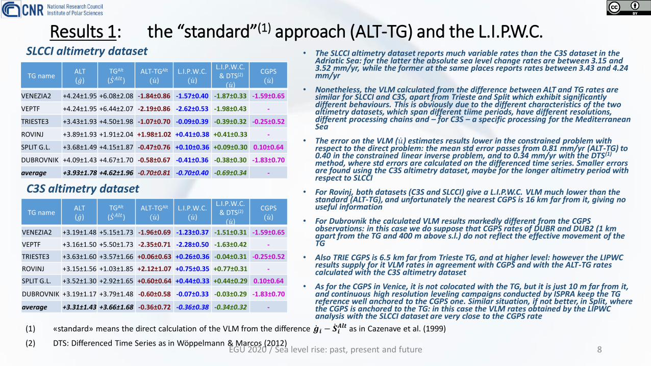
• The SLCCI altimetry dataset reports much variable rates than the C3S dataset in the Adriatic Sea: for the latter the absolute sea level change rates are between 3.15 and 3.52 mm/yr, while the former at the same places reports rates between 3.43 and 4.24 mm/yr

• Nonetheless, the VLM calculated from the difference between ALT and TG rates are similar for SLCCI and C3S, apart from Trieste and Split which exhibit significantly different behaviours. This is obviously due to the different characteristics of the two altimetry datasets, which span different tiime periods, have different resolutions, different processing chains and – for C3S – a specific processing for the Mediterranean Sea

• The error on the VLM ( 𝑢) estimates results lower in the constrained problem with respect to the direct problem: the mean std error passes from 0.81 mm/yr (ALT-TG) to 0.40 in the constrained linear inverse problem, and to 0.34 mm/yr with the DTS(1)

method, where std errors are calculated on the differenced time series. Smaller errors are found using the C3S altimetry dataset, maybe for the longer altimetry period with respect to SLCCI

• For Rovinj, both datasets (C3S and SLCCI) give a L.I.P.W.C. VLM much lower than the standard (ALT-TG), and unfortunately the nearest CGPS is 16 km far from it, giving no useful information

• For Dubrovnik the calculated VLM results markedly different from the CGPS observations: in this case we do suppose that CGPS rates of DUBR and DUB2 (1 km apart from the TG and 400 m above s.l.) do not reflect the effective movement of the TG

• Also TRIE CGPS is 6.5 km far from Trieste TG, and at higher level: however the LIPWC results supply for it VLM rates in agreement with CGPS and with the ALT-TG rates calculated with the C3S altimetry dataset

• As for the CGPS in Venice, it is not colocated with the TG, but it is just 10 m far from it, and continuous high resolution leveling campaigns conducted by ISPRA keep the TG reference well anchored to the CGPS one. Similar situation, if not better, in Split, where the CGPS is anchored to the TG: in this case the VLM rates obtained by the LIPWC analysis with the SLCCI dataset are very close to the CGPS rate

(1) «standard» means the direct calculation of the VLM from the difference 𝒈𝒊 − 𝑺𝒊𝑨𝒍𝒕 as in Cazenave et al. (1999)

(2) DTS: Differenced Time Series as in Wöppelmann & Marcos (2012)

Results 2: the L.I.P.W.C. + the bias method 1 (“fake” bias)SLCCI altimetry dataset



TG nameALT-TGAlt

( 𝑢)L.I.P.W.C.

( 𝑢)L.I.P.W.C.

& DTS(1) ( 𝑢)L.I.P.W.C. + bias 1 ( 𝑢)

L.I.P.W.C. + bias 1 & DTS(1) ( 𝑢)

CGPS( 𝑢)

VENEZIA2 -1.96±0.69 -1.23±0.37 -1.51±0.31 -1.23±0.37 -1.51±0.31 -1.59±0.65

VEPTF -2.35±0.71 -2.28±0.50 -1.63±0.42 -2.28±0.48 -1.63±0.42 -

TRIESTE3 +0.06±0.63 +0.26±0.36 -0.04±0.31 +0.26±0.37 -0.04±0.31 -0.25±0.52

ROVINJ +2.12±1.07 +0.75±0.35 +0.77±0.31 +0.75±0.35 +0.77±0.31 -

SPLIT G.L. +0.60±0.64 +0.44±0.33 +0.44±0.29 +0.44±0.34 +0.44±0.29 0.10±0.64

DUBROVNIK -0.60±0.58 -0.07±0.33 -0.03±0.29 -0.07±0.34 -0.03±0.29 -

average -0.36±0.72 -0.36±0.38 -0.34±0.32 -0.36±0.38 -0.34±0.32 -0.58±0.60

TG nameALT-TGAlt

( 𝑢)L.I.P.W.C.

( 𝑢)L.I.P.W.C.

& DTS(1) ( 𝑢)L.I.P.W.C. + bias 1 ( 𝑢)

L.I.P.W.C. + bias 1 & DTS(1) ( 𝑢)

CGPS( 𝑢)

VENEZIA2 -1.84±0.86 -1.57±0.40 -1.87±0.33 -1.57±0.42 -1.87±0.33 -1.59±0.65

VEPTF -2.19±0.86 -2.62±0.53 -1.98±0.43 -2.62±0.51 -1.98±0.43 -

TRIESTE3 -1.07±0.70 -0.09±0.39 -0.39±0.32 -0.09±0.42 -0.39±0.32 -0.25±0.52

ROVINJ +1.98±1.02 +0.41±0.38 +0.41±0.33 +0.41±0.40 +0.41±0.33 -

SPLIT G.L. -0.47±0.76 +0.10±0.36 +0.09±0.30 +0.10±0.39 +0.09±0.30 0.10±0.64

DUBROVNIK -0.58±0.67 -0.41±0.36 -0.38±0.30 -0.41±0.39 -0.38±0.30 -

average -0.70±0.81 -0.70±0.40 -0.69±0.34 -0.70±0.42 -0.69±0.34 -0.58±0.60

In the table we report the results obtained using the “fake” bias (bias method 1; in red and blue) alongside the ALT-TG and L.I.P.W.C.&DTS methods already shown in the previous slide, for comparison

• The errors are generally lower in the DTS counterpart of the calculated rates, as expected.

• Taking as indicators Venice and Split, which have the most adequate locations of the CGPS stations, the SLCCI dataset seems to give the best agreement in terms of VLM rates, with the LIPWC&DTS method, irrespective of the introduction of the fake bias, while the C3S dataset ensures the lowest errors, maybe for the longest time span, 13% longer than SLCCI

• The results of the SLCCI dataset seem to better reflect the rates calculated by the CGPS stations near the VENEZIA2, TRIESTE3 and SPLIT G.L. TG

• The results of the “fake” bias method seem indistinguishable from the corresponding results of L.I.P.W.C. without bias (orange and pale blue); however the bias should have granted the validity of eg. b) irrespective of the choice of the TG-TG couple: one could ask himself which benefit brings the introduction of the “bias” in the calculation. The answer is not easy as the biases have been introduced in order to cancel the dependence of the TG relative sea level rates from the absolute sea level seen at the tide gauge. However, no evidence are seen that this happens. Anyway, the two bias methods are seen to maintain the invariance of the LIPWC method to independent permutations of the TG-TG couples, confirming that the biases are correctly formulated in the calculations

• This holds true as long as the LIPWC method is used without the DTS: the reason is obvious: both errors calculated with the covariance matrix and DTS are non-linear in the rates, and specifically in the biases. The non-linearity of the DTS calculation brings asymmetry, and thus breaks the invariance w.r.t. permutations of the TG-TG couples


Results 3: the L.I.P.W.C. + the bias method 2SLCCI altimetry dataset



• The table shows the results obtained using the second bias method (bias method 2; in red and blue) alongside the ALT-TG and L.I.P.W.C.&DTS methods already shown in the previous slides, for comparison. The results of the bias 2 method, in contrast with the bias 1 method, are different from the corresponding results of L.I.P.W.C. without bias (orange and pale blue), but still, the invariance w.r.t. independent permutations of the TG in the constraints is maintained. Errors instead change magnitude, due to the non-linearity in the std error of the covariance matrix

• The bias 2 method provides VLM rates less similar to the CGPS observations (VENEZIA2, TRIESTE3 and SPLIT G.L.), even if the averages (last row) are identical to those of the bias 1 method


TG nameALT-TGAlt

( 𝑢)L.I.P.W.C.

( 𝑢)L.I.P.W.C.

& DTS(1) ( 𝑢)L.I.P.W.C. + bias 2 ( 𝑢)

L.I.P.W.C. + bias 2 & DTS(1) ( 𝑢)

CGPS( 𝑢)

VENEZIA2 -1.96±0.69 -1.23±0.37 -1.51±0.31 -1.35±0.38 -1.63±0.31 -1.59±0.65

VEPTF -2.35±0.71 -2.28±0.50 -1.63±0.42 -2.43±0.52 -1.78±0.42 -

TRIESTE3 +0.06±0.63 +0.26±0.36 -0.04±0.31 +0.58±0.38 +0.28±0.31 -0.25±0.52

ROVINJ +2.12±1.07 +0.75±0.35 +0.77±0.31 +0.60±0.36 +0.61±0.31 -

SPLIT G.L. +0.60±0.64 +0.44±0.33 +0.44±0.29 +0.65±0.35 +0.65±0.29 0.10±0.64

DUBROVNIK -0.60±0.58 -0.07±0.33 -0.03±0.29 -0.19±0.35 -0.14±0.29 -

average -0.36±0.72 -0.36±0.38 -0.34±0.32 -0.36±0.39 -0.34±0.32 -0.58±0.60

TG nameALT-TGAlt

( 𝑢)L.I.P.W.C.

( 𝑢)L.I.P.W.C.

& DTS(1) ( 𝑢)L.I.P.W.C. + bias 2 ( 𝑢)

L.I.P.W.C. + bias 2 & DTS(1) ( 𝑢)

CGPS( 𝑢)

VENEZIA2 -1.84±0.86 -1.57±0.40 -1.87±0.33 -1.25±0.42 -1.55±0.33 -1.59±0.65

VEPTF -2.19±0.86 -2.62±0.53 -1.98±0.43 -2.30±0.54 -1.67±0.43 -

TRIESTE3 -1.07±0.70 -0.09±0.39 -0.39±0.32 -0.59±0.41 -0.90±0.32 -0.25±0.52

ROVINJ +1.98±1.02 +0.41±0.38 +0.41±0.33 +0.38±0.40 +0.38±0.33 -

SPLIT G.L. -0.47±0.76 +0.10±0.36 +0.09±0.30 -0.15±0.39 -0.17±0.30 0.10±0.64

DUBROVNIK -0.58±0.67 -0.41±0.36 -0.38±0.30 -0.25±0.39 -0.23±0.30 -

average -0.70±0.81 -0.70±0.40 -0.69±0.34 -0.70±0.42 -0.69±0.34 -0.58±0.60

Results 4: the L.I.P.W.C. and the bias method 1&2: a metrics SLCCI altimetry dataset



To understand which analysis method is better, and which altimetry dataset provides more coherent rates, we introduce a metric based on three indexes 𝜹𝒊:

1. 𝜹𝟏: the RMSD of the ALT-TG rates and the “METHOD” rates, where “METHOD” is one of the six analyzed in this study, namely L.I.P.W.C., L.I.P.W.C. DTS, …

2. 𝜹𝟐: the RMSD of the CGPS rates and the “METHOD” rates, limited to the three CGPS stations which are coherent with the ALT-TG rates (VENEZIA PSAL, TRIESTE TRIE, SPLIT)

3. 𝜹𝟑: the mean of the std deviations associated with the METHOD (<σ(METHOD)>)

From these three indexes the lowest square root of the sum of the squares is taken as the “overall” index Δ. The red squares identify, for each altimetry dataset, the analysis methods with lowest Δ. The formulation consisting in the solution of the linear inverse problem with constraints (LIPWC) where TG-TG and ALT-TG rates are calculated by differentiation of the time series of SL higth (DTS) with and without bias (method 1 – fake bias) show the best score.

METHOD «X» RMSD(X,ALT-TGAlt)

𝜹𝟏

RMSD(X,CGPS)𝜹𝟐

<σ(X)>𝜹𝟑

∆=2

𝑖=1

3

𝛿𝑖2

LIPWC 0.68 0.41 0.38 0.88

LIPWC DTS 0.70 0.24 0.32 0.81

LIPWC b1 0.68 0.41 0.38 0.88

LIPWC b1 DTS 0.70 0.24 0.32 0.81

LIPWC b2 0.72 0.59 0.39 1.01

LIPWC b2 DTS 0.70 0.44 0.32 0.89

METHOD «X» RMSD(X,ALT-TGAlt)

𝜹𝟏

RMSD(X,CGPS)𝜹𝟐

<σ(X)>𝜹𝟑

∆=2

𝑖=1

3

𝛿𝑖2

LIPWC 0.82 0.10 0.40 0.92

LIPWC DTS 0.74 0.18 0.34 0.83

LIPWC b1 0.82 0.10 0.42 0.93

LIPWC b1 DTS 0.74 0.18 0.34 0.83

LIPWC b2 0.75 0.31 0.42 0.91

LIPWC b2 DTS 0.73 0.40 0.34 0.90

SummaryWe have estimated trends and errors at six locations in the Adriatic Sea; we have used three different measuring systems (tide gauges, radar altimetry, continuous gps), integrating the information coming from each of the three system, in order to maximize the knowledge, qualitatively and quantitatively. We have assessed two different altimetry products (ESA SLCCI and Copernicus C3S) specifically processed for climate studies. We have compared the results with the direct method (subtracting the relative from the absolute sea level rates) and as a constrained linear inverse problem, which permits to simoultaneously solve for the rates of all TGs. We also tested the robustness of the constrained linear inverse problem with respect to a known limitation.

We found that:

• The two altimetry products, SLCCI and C3S, supply very similar results: errors on the calculated VLM rates are slightly lower for the C3S dataset, which cover a period 13% longer w.r.t. SLCCI

• The simoultaneous solution of the VLM rates with the constrained linear inverse problem, where the TG-TG and the ALT-TG rates were calculated by differencing the time series of sea level, had the best performance, both in the simple formulation and using a «fake» bias (bias method 1). The errors on the VLM rates are of the order of 0.3-0.4 mm yr-1

• The use of biases does not bring any improvement in the derived rates and errors: this could suggest that the LIPWC method is robust enough not to suffer from deviation from the rule 𝑔𝑖 − 𝑔𝑗 = 0

• Overall, for the Adriatic Sea we obtain a consistent representation of the absolute and relative sea level change rates , from altimetry and tide gauges, but with a little difference which can be explained by the vertical motion of TGs, moving with mean rate of 0.35-0.70 mm yr-1, but with different rates and signs from place to place. These rates are confirmed by the derived mean rates from 3 CGPS stations

To be considered:

• The SLCCI and C3S datasets cover slightly different periods

• The SLCCI and C3S products are generated from different processing chains, have different spatial and temporal resolutions, and C3S relies on a mapping algorithm specifically dedicated to the Mediterranean Sea

• GPS data span very different time periods, but always shorter than altimetry and TGs time series; sometimes it is difficult to understand if CGPS stations do effectively reflect the tide gauge movement

Open questions:

• Open question 1: can we use this strategy to analyze sea level rates in other regions of the Mediterranean Sea or elsewhere?

• Open question 2: how can we maximize the exploitation of the existing CGPS stations in this context, and improve the integration of the available measurement systems?


estimating vertical land motion in northern adriatic sea with … · 2020-04-29 · estimating...

Documents