estimating the value of service using load forecasting models valu… · · 2017-07-12estimating...

1

Estimating the Value of Service Using Load Forecasting Models

Richard Stevie, Integral Analytics Jose Merino, Duke Energy

Ken Skinner, Integral Analytics Raiford Smith, Duke Energy

Eric Woychik, Strategy Integration, LLC.

Presented at the May 2014 Eastern Conference – Center for Research in Regulated Industries

1. Introduction

What is the actual value of electric service to customers? In this light, what is the optimal level of

investment in generation, transmission, and distribution? What is the value of electricity reliability?

These are complex and difficult questions for utility planners, executives, and regulatory agencies.

Estimates of the Value of Service (VOS) provide critical information to support customer-focused, value-based planning. VOS is particularly useful to determine the economically efficient level of investment in utility plant (generation, transmission, and distribution). VOS can also be used to evaluate the payoff for investments in technologies to better manage the grid, improve reliability, and provide service quality. The importance of reliability continues to grow rapidly with greater reliance on the internet economy and its associated dependence on a safe and reliable electric supply. Reliable estimates of VOS have been difficult to determine given the number of parameters involved and the uncertainties that arise from the use of survey techniques. Planners have used integrated resource planning models (IRP) to design resource plans to minimize long-run revenue requirements subject to reliability criteria on number of hours of unserved energy and/or reserve margins. However, these values are not grounded with a customer VOS perspective. These models tend to produce only macro, high-level values for large assets such as central-station generation or transmission. Furthermore, these models fail to consider costs or benefits beyond those directly attributable to a utility asset. Most VOS calculations rely on primary market research. These techniques either directly elicit customer estimates of the value lost from outages (e.g. willingness-to-accept compensation for an outage) or use methods to identify customer investments to reduce the impact of future outages (e.g. willingness-to-pay to avoid a negative outcome). In regulatory settings, VOS usually receives less focus compared to the utility’s cost-of-service (COS) because COS is easier to quantify. Thus, avoided cost of service, defined in marginal terms, has been the primary metric for judging investment decisions in regulated utility arenas. While VOS techniques have been in use for decades, regulators have used VOS estimates primarily to define reliability levels, such as the U.K.’s use of Value-of-Lost-Load (VOLL). There is general agreement that VOS produces greater values than COS, including when customer survey techniques are used. The accepted approach in advanced resource planning is to equate the marginal VOS to the marginal COS (MVOS = MCOS), as this represents the “market” equilibrium point where the marginal customer value is equal to the marginal cost of providing that value. In order to reduce the uncertainty in current VOS estimates, this paper presents a valuation approach to augment existing primary market research techniques. Economic theory shows that the consumer

2

demand curve represents the consumers’ willingness to pay for an assumed quantity demanded. Thus, the area under the demand curve for electricity offers an estimate of consumer value for the use of electricity. This paper uses econometric load forecasting models to demonstrate an alternate method for determining class level VOS estimates for customer use of electricity. While the proposed method brings with it uncertainty, the use of multiple estimates - both survey-based and demand curve-based- coupled with methods to capture covariance of key variables (such as weather, economics, prices, and customer behavior), enables a comparison of results and should increase the confidence in the use of VOS estimates. The paper proceeds with a brief review of the literature. That leads to a discussion on the load forecasting model and the process used to estimate VOS. From this, estimates of the VOS are provided for customer classes in the Duke Energy Carolina service area. These estimates are then compared to estimates derived from past VOS survey research. Finally, detailed recommendations are offered on grid-based data collection needs to extend VOS calculations for individual customers.

2. Literature

Several attempts have been made in the literature to develop estimates of VOS1. Eto (2001) provides a

good review of past research into this field. Generally, past studies have been survey based; that is, they

have relied upon primary research surveys of customers to obtain their views on the value of reliable

electricity service. The focus of the surveys has been two-fold: obtain estimates of the costs imposed

from past load interruptions and obtain estimates of customer willingness to pay to avoid an

interruption / the amount they would accept in compensation for an interruption.

A study by Sullivan, et al. (2009)2 provides a methodology for developing estimates based upon a meta-

analysis of survey data collected through past primary research studies. After collecting survey results

from 28 studies of utility customer views from across the United States, Sullivan, et al. (2009)

implemented an econometric based approach to estimating damage functions. These damage functions

were designed to capture differences in customer characteristics, interruption attributes, and

environment or climate conditions. In addition, the damage functions also allow for differentiation of

the estimates by regions of the country.

1 Reports to note: J Eto, J Koomey, B Lehman, N Martin, E Mills, C Webber, and E Worrell, “Scoping Study on

Trends in the Economic Value of Electricity Reliability to the U.S. Economy.” LBNL Report No. LBNL-47911 (2001); L Lawton, M Sullivan, K Van Liere, A Katz, and J Eto. “A framework and review of customer outage costs: integration and analysis of electric utility outage cost surveys.” LBNL Report No. LBNL-54365. (November 2003); Kristina Hamachi LaCommare and Joseph H. Eto. “Understanding the Cost of Power Interruptions to U.S. Electricity Consumers,” LBNL Report No. LBNL-55718 (September 2004); London Economics. “Estimating the Value of Lost Load: Briefing paper prepared for the Electric Reliability Council of Texas, Inc.” London Economics International LLC (June 17th, 2013); The Brattle Group “Approaches to setting electric distribution reliability standards and outcomes,” The Brattle Group, Ltd. (January 2012); and Michael J. Sullivan, Matthew Mercurio, and Josh Schellenberg. “Estimated Value of Service Reliability for Electric Utility Customers in the United States” LBNL Report No. LBNL-2132E (June 2009). 2 Michael J. Sullivan, Matthew Mercurio, and Josh Schellenberg (June 2009).

3

In a recent report conducted for ERCOT, London Economics (2013) provided a critical review of past

research into VOS3. In addition to acknowledging the difficulty associated with customers developing

their own VOS estimates, London Economics (2013) points out that VOS estimates are extremely

sensitive to factors like customer type, outage duration, time of an outage, and advance notification of

an outage.

In the London Economics (2013) report, past study methodologies are categorized into four groups:

revealed preference (past spending to avoid interruption), stated choice surveys (contingent valuation

and conjoint), macroeconomic estimates (e.g., GDP/MWH), and case studies (review impact of actual

events). While each of these approaches is useful and can help triangulate on potentially reasonable

VOS estimates, London Economics (2013) points out the weaknesses of each.

For example, the revealed preference approach, while using actual customer data, is only relevant if

customers actually invested to mitigate exposure to interruptions. This limits the applicability of the

approach. The stated preference method relies on consumer responses to surveys. While survey

questions allow for more input on aspects such as the impact of outage duration, the results can be

unreliable since consumers may not be able to reasonably relate their perception of the impact of

outages to monetary values. The macroeconomic approach may be easy to implement, but represents

too broad of a measurement. And finally, the use of case studies can provide great insights, but the

results are costly to obtain and have limited applicability to a general understanding of the VOS.

London Economics (2013) concludes that estimating VOS is a challenging task that ultimately requires

the use of a survey of customers. Past research into VOS has typically been based on primary research

of customers. Estimates have not been attempted through the use of load forecasting demand

functions.

3. A New VOS Approach

In economic theory, the demand curve for a good or service represents what a consumer is willing to

pay for a certain quantity of a good or service at a given price. For electricity markets, if a consumer

only consumes one kWh, the demand curve will represent the maximum amount that the consumer

would pay for one kWh4. In that context, this equates to the VOS associated with the consumption of

that first kWh. Obviously, electricity users consume a lot more than one kWh. But, at a given price for

electricity, the area under the demand curve for the volume of kWh consumed at that going price will

represent the VOS for that volume of consumption.

3 The London Economics (2013) study actually focused on the value of lost load (VOLL) which is another way to

examine VOS. 4 See page 99 of Edwin Mansfield. Microeconomics, 6

th Edition. New York: W.W. Norton & Company, 1988 for a

discussion of consumer surplus. While this is not the same as willingness to accept compensation, the area under the demand curve represents the implied value from consumption of the good as an alternate measure to survey based estimates of value.

4

Given a demand curve for electricity like that shown in Figure 1 below, the area identified by ABCD

represents the value of the service (VOS) to the consumer. Note this area is larger than just the area

found by multiplying the price times the quantity since it also includes consumer surplus.

Now, using an econometric model of the demand curve, the VOS can be estimated at the margin and in

total. The value along the line AB represents the VOS of the marginal unit. If a consumer is forced to

reduce usage, the marginal VOS would be expected to increase (the value on the line increases as Q

declines).

Taking a residential demand equation such as this:

(1) Q = a + b P + c Income + d W + ɛ

where:

Q = quantity or kWh

P = price per unit

Income = consumer income

W = weather and any other variables

a = intercept

b, c, & d = slope parameters

ɛ = error

5

The inverse of the equation becomes:

(2) P(Q) = (Q – a - c Income - d Weather)/b

Then, the VOS area can be estimated by taking the integral of the demand equation for the volume of

consumption.

(3) ( ) ((Q – a - c Income - d Weather)/b) dQ

From (3), one can take the value of the integral over the range to the quantity consumed and divide by

the volume to get an average VOS/kWh. However, it will be important to show how the integral

changes as quantity Q declines and how the VOS/Q changes with marginal changes in Q.

For electricity, a number of factors impact the level of consumption. For example, a residential

customer’s usage will vary depending upon factors such as: income level, the efficiency of the appliances

in the home, the weather, the size and thermal integrity of the home, and the type of appliances being

used. Similarly, a commercial customer’s usage will vary significantly based upon factors such as: the

type of business, the size of the building, the efficiency of the equipment in the business, the volume of

business, and the number of employees. Industrial or manufacturing facilities possess the most

variability when one considers how much end-user energy consumption can change from one industry

to another. In addition to the same types of factors affecting commercial usage, the type of industry

plays a major role in the amount of energy consumption. For example, steel plants and chemical

6

manufacturers will typically use a lot more energy than a furniture factory. However, customer energy

use (even within the same industry) still depends on the relative sizes of the facilities.

As part of the utility planning process, electric utilities prepare forecasts of future energy usage by

customer class. These forecasts often look twenty to thirty years into the future. Over the past few

decades, the methodology employed to prepare a forecast has evolved from simple trend lines to

econometric models, to end-use models, to hybrid econometric/end-use models and statistically-

adjusted end-use (SAE) models. One feature of econometric based forecasting models is these models

can provide an alternate view of the VOS. In the process of estimating price elasticity, the econometric

based electric load forecasting model represents the demand curve for electricity, holding other

variables constant. Using equations (1) through (3) above, one can employ the coefficients from a load

forecasting model to estimate the VOS. This forms the basis for the following process of VOS estimation

using actual demand forecasting models of Duke Energy Carolinas.

4. VOS Application Using Duke Energy Carolinas’ Forecasting Models

Duke Energy Carolinas has prepared load forecasts for decades using econometric based models. The

general model structure involves the development of econometric models for each class: residential,

commercial, and industrial. The industrial class includes models for major industry groups, e.g.,

chemical, primary metals, textiles, etc. Using the forecasting models for the residential and commercial

classes, as well as for one of the major industry groups, we can estimate VOS as implied by the estimate

of the demand function. For Duke Energy Carolinas, the residential sector is modeled linearly on a use

per customer basis. For the commercial sector and the industry group, electric usage is modeled for the

total class or group using a log-linear relationship. These modeling differences can impact the shape of

the estimates, though the processes are similar5. Table 1 provides the coefficient estimates for each of

the models.

5 The integration for the linear model is more straightforward than that for the log-linear model.

Residential kWh/Customer/Day LN(Commercial MWH) LN(Industrial MWH)

Intercept 16.24

Heating Degree Days 0.014297476

Cooling Degree Days 0.024556869

Appliance Stock x Real Disposable Income/Capita (1) 0.0000000145188269194

Appliance Stock x Real Electric Price (1) (0.0000437023704676)

Real Price of Natural Gas 0.140737168

Intercept 5.351481587 8.997335708

Heating Degree Days (2) 0.00004399967 (0.00004864)

Cooling Degree Days 0.000293522 0.00005427

LN(Real Disposable Income) 0.853974652

LN(Real Electric Price) -0.240285671 -0.312070781

LN(Real Gross Domestic Product for NAICS 325) 0.496976457

(1) Applicance stock represents an appliance saturation and efficiency weighted level of connected appliance load.

(2) Note: the coefficient in the industrial model for HDD is negative inducating the presence generation on-site that

operates during colder weather.

Table 1

Coefficient Estimates

7

Residential VOS per Customer

Using the model coefficients, we estimate the VOS for an average residential customer in the Duke

Energy Carolinas service area as shown in Table 2.

This table shows how the residential consumer’s VOS varies by season6. These are average values for

the season. As one would expect, usage in the seasons with greater exposure to extreme weather are

valued higher. All VOS values have been converted to a 2014 dollar level.

Going further, one can see from Tables 3 to 5 how the estimates vary with the weather and with income

levels. Table 3 provides estimates as the level of HDD increases, whole Table 4 presents similar

information over a range of CDD values. Table 5 provides a view into how VOS adjusts with alternate

levels of income.

6 The seasonal reference is an approximation. The seasons actually represent the four quarters of the year. These

approximate the seasons since, for example, the billing degree days for the first quarter (January through March) would actually include a major portion of December.

kwh VOS VOS Cents

Season per Day $ per Day per kWh

Winter 42.25 21.99 52.05

Spring 31.36 12.53 39.98

Summer 42.37 22.06 52.08

Fall 32.92 13.71 41.65

Estimates of Residential Value of Service

Table 2

kwh VOS VOS Cents

HDD per Day $ per Customer/Day per kWh

0 19.98 5.47 27.37

100 21.41 6.20 28.95

500 27.12 9.56 35.25

1000 34.27 14.79 43.14

1500 41.42 21.14 51.03


Table 3

8

As expected, Table 5 shows how the VOS increases with income. It should be noted that one cannot tell

if summer usage is valued more than winter usage due to the fact that the levels of HDD and CDD have

different levels of importance that can be affected by the saturation of electric heat vs. air conditioning.

To truly understand the differential valuation would require conducting this type of analysis at the

individual level for those with gas heat and central air as well as those with electric heat and central air.

This will be discussed further in the section on potential extensions of this type of analysis.

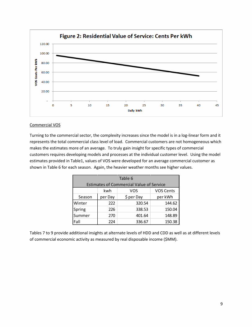
Figure 2 below provides a visual look at how the VOS per kWh varies with the level of daily usage. This is

looking that the VOS during a winter season. The implication is that those first few kWh are valued a lot

higher than at the point where the consumer already has a positive level of consumption.

kwh VOS VOS Cents

CDD per Day $ per Day per kWh

0 19.98 5.47 27.37

100 22.43 6.75 30.08

200 24.89 8.16 32.79

500 32.25 13.20 40.91

1000 44.53 24.25 54.46


Table 4

kwh VOS VOS Cents

Season Income per Day $ per Day per kWh

Winter 30,000$ 41.42 21.14 51.03

Winter 50,000$ 45.15 24.90 55.14

Winter 100,000$ 54.47 35.64 65.42

Summer 30,000$ 39.62 19.43 49.04

Summer 50,000$ 43.35 23.04 53.15

Summer 100,000$ 52.67 33.41 63.44


Table 5

9

Commercial VOS

Turning to the commercial sector, the complexity increases since the model is in a log-linear form and it

represents the total commercial class level of load. Commercial customers are not homogeneous which

makes the estimates more of an average. To truly gain insight for specific types of commercial

customers requires developing models and processes at the individual customer level. Using the model

estimates provided in Table1, values of VOS were developed for an average commercial customer as

shown in Table 6 for each season. Again, the heavier weather months see higher values.

Tables 7 to 9 provide additional insights at alternate levels of HDD and CDD as well as at different levels

of commercial economic activity as measured by real disposable income ($MM).

kwh VOS VOS Cents


Winter 222 320.54 144.62

Spring 226 338.53 150.04

Summer 270 401.64 148.89

Fall 224 336.67 150.38

Estimates of Commercial Value of Service

Table 6

10

Tables 7 and 8 demonstrate how the VOS for an average commercial customer increases as the effect of

weather rises. And, Table 9 provides insight on how that VOS rises as the level of commercial economic

activity ramps up.

The VOS for an average commercial customer for the daily level of kWh is provided in Figure 3. Notice

the curvature of this result relative to that in the residential model. This is a direct outcome of the

underlying functional form of the forecasting equation, linear vs. log-linear.

Kwh per Day VOS

HDD per Customer $ per Customer/ Day

0 208.0 309.09

100 208.9 310.46

500 212.7 315.97

1000 217.4 323.00

1500 222.2 330.18

Table 7


Kwh per Day VOS

CDD per Customer $ per Customer/ Day

0 208.03 249.67

100 214.22 257.11

200 220.60 264.77

500 240.91 289.14

1000 278.99 334.84

Table 8


Regional kwh VOS

Season Disposable Income per Day $ per Customer/ Day

Winter 200,000$ 252.35 302.87

Winter 250,000$ 305.32 366.45

Winter 300,000$ 356.76 428.18

Summer 200,000$ 213.15 255.82

Summer 250,000$ 257.90 309.52

Summer 300,000$ 301.34 361.67


Table 9

11

Industrial VOS

Duke Energy Carolinas has developed econometric based forecasting models for many industry groups.

For this research, the purpose here is to show that the process of using econometric forecasting models

can be applied to derive estimates of the VOS. The chemical industry is one of the key industries within

the Duke Energy Carolinas service area. For that reason, the forecasting model for the chemical industry

is utilized to derive industrial VOS estimates realizing that these values do not reflect the full industrial

sector.

As with the commercial class, the chemical industry sector is not homogeneous. Customers can vary

greatly in size, even though they may be classified in the same industry. As before, to truly understand

the VOS for the industry requires investigating this at the customer level. Using the log-linear model

coefficient estimates provided in Table10, values of VOS were developed for an average chemical

industry customer as shown in Table 6 for each season.

While the VOS cents per kWh estimates are much lower than those for an average commercial

customer, due to the higher volumes, the VOS daily values are much higher. This indicates that the

industrial customer might have more options to adjust to a minor reduction in usage, but that a total

shut-down has more serious consequences.

kwh VOS VOS Cents


Winter 13,337 7,386 55.38

Spring 14,768 8,212 55.61

Summer 15,631 8,766 56.08

Fall 14,292 7,810 54.65

Estimates of Industrial Value of Service

Table 10

12

Tables 11 to 13 provide additional insights at alternate levels of HDD and CDD as well as at different

levels of industrial economic activity as measured by real gross domestic product for the chemical

industry ($MM).

Tables 11 and 12 demonstrate how the VOS for an average chemical industry customer changes with the

severity of the weather. As previously noted, decreases in VOS are associated with an increase in HDD.

This occurs because chemical companies’ need to turn on alternate generating facilities to create steam

which can produce electricity as a by-product, hence reducing dependence on utility provided

generation. The converse occurs for CDD. Table 13 provides insight on how that VOS rises as the level

of industrial economic activity increases.

Kwh per Day VOS

HDD per Customer $ per Customer/Day

0 14,650.2 8,357$

100 14,579.1 8,317$

500 14,298.1 8,156$

1000 13,954.6 7,960$

1500 13,619.3 7,769$

Table 11


Kwh per Day VOS

CDD per Customer $ per Customer/Day

0 14,650.15 8,357

100 14,729.88 8,403

200 14,810.05 8,448

500 15,053.17 8,587

1000 15,467.26 8,823

Table 12


kwh VOS

Season Real GDP NAICS 325 per Day $ per Customer/Day

Winter 7,000$ 14,784.55 8,433.82

Winter 7,500$ 15,300.27 8,728.01

Winter 8,000$ 15,798.97 9,012.49

Summer 7,000$ 13,160.20 7,507.21

Summer 7,500$ 13,619.26 7,769.08

Summer 8,000$ 14,063.16 8,022.30


Table 13

13

The VOS for an average chemical industry customer for the daily level of kWh is provided in Figure 4. As

for the commercial class, there is a similar curvature to this relationship. This is a direct outcome of the

underlying log-linear functional form of the forecasting equation.

5. Comparison to an Alternate View

The approach conducted in the Sullivan, et al. (2009)7 study produced estimates of the VOS for three

classes: residential customers, small commercial and industrial (C&I) customers, and medium and large

C&I customers. While the categories may be different and the lengths of outages do not necessarily

correspond to the values developed above, they do provide an opportunity for comparison.

Table 14 is taken from the Sullivan, et al. (2009)8 study. It provides estimates of the VOS for each of the

customer groups at different levels of outage. Keep in mind that Sullivan, et al. (2009) focused on

estimating damage functions to represent the VOS as viewed by a customer facing an outage. The

values in the table are in 2008$. These have to be adjusted for inflation between 2008 and 2014 to

make them comparable to the dollar values derived from the econometric forecasting models presented

in the previous tables.

7 See Michael J. Sullivan, Matthew Mercurio, and Josh Schellenberg (June 2009).

8 See Michael J. Sullivan, Matthew Mercurio, and Josh Schellenberg (June 2009), page xxvi.

14

Table 14

The load forecasting models used in developing VOS estimates in this paper reflect an implied VOS.

Table 15 provides a summary comparison of the range of values from the Sullivan, et al. (2009) versus

those derived from the load forecasting models.

The comparison of these results reveals the following:

The residential model based estimates far exceed those from the Sullivan Study. The model

based estimates are intended to reveal implied value, while the Sullivan Study estimates are

based on market research. This may point to the difficulty of obtaining a residential customer’s

estimate of damage through a survey.

Class Momentary 1 Hour 8 Hours Class

Residential 2.36$ 3.71$ 11.91$ Residential 19.43$ 54.46$

Small C&I 329.18$ 695.44$ 5,836.56$ Commercial 255.82$ 428.18$

Medium and Large C&I 7,367.89$ 14,029.09$ 77,840.29$ Industrial 7,507.21$ 9,012.49$

Note: All values are in 2014 $.

Cost Per Event VOS Estimates Model Based Implied VOS Estimates

Sullivan Study Forecast Model

Cost Per Day Range

Table 15

VOS Estimate Comparisons

15

The small C&I and the medium and large C&I estimates for a momentary outage from the

Sullivan Study seem to correlate well with the commercial and industrial model based estimates.

The small C&I and the medium and large C&I estimates for longer periods of time from the

Sullivan Study far exceed the model based estimates. However, the model based estimates

reflect an average value over a quarter assuming a normal daily level of usage. The model based

value of service can increase dramatically into the tens of thousands of dollars for commercial

and industrial customers if the customer can only obtain 10 percent of their normal level of

energy. In that case, the customer places a high value on an incremental amount of energy.

6. Conclusion and Potential for Future Research

The research presented in this paper provides an alternate approach for estimating the VOS using utility

forecasting models. While the results found here just scratch the surface, they do point to a reasonable

method for utilities to obtain estimates of the VOS. The advantages of this approach are that it is a less

costly method than primary research and it provides an implied customer perception of value that

survey methods cannot provide. At the same time, survey based methods possess more flexibility for

assessing perceptions that vary over the length of an outage. The bottom line is that both methods can

be useful in triangulating on a concept that is very difficult to estimate.

Further gains in the model based approach are readily apparent. By developing econometric models of

consumer demand for sub-groups of customers (e.g., residential space heating, residential air

conditioning, and any number of types of commercial and industrial customers), one can easily obtain

detailed estimates of the implied VOS. Data from load research studies that collected interval data

could be used to examine the hourly level of the VOS. Data from utility residential customer appliance

saturation surveys could also be used to further understand how the VOS varies based upon the nature

of the individual customer’s appliance ownership as well as type of residence and economic situation.

Other segments or characteristics that could be examined include customers in Energy Star certified

buildings, customers in older traditional buildings, and impacts of alternate rate designs.

Ultimately, with the collection of more granular data on all customers through smart grid applications

and data collection processes, it would be possible to estimate the VOS for each customer. For utilities,

this becomes extremely important for identifying those customers that place greater value on service

and reliability than others. This impacts the locational need for distribution system upgrades and can

help identify those customers more likely to participate in energy efficiency and demand response

programs as well as those more likely to be interested in distributed energy resources including storage

and renewable sources of energy.

16

References:

1. The Brattle Group. “Approaches to setting electric distribution reliability standards and outcomes.” (January 2012). The Brattle Group, Ltd.

2. Eto, J.; Koomey, J.; Lehman,B.; Martin, N.; Mills, E.; Webber, C.; and Worrell, E. Scoping Study on Trends in the Economic Value of Electricity Reliability to the U.S. Economy. (LBNL Report No. LBNL-47911, 2001). Lawrence Berkeley National Laboratory, Berkeley, California.

3. LaCommare, Kristina Hamachi and Eto, Joseph H. Understanding the Cost of Power Interruptions to U.S. Electricity Consumers. (LBNL Report No. LBNL-55718, September, 2004). Lawrence Berkeley National Laboratory, Berkeley, California.

4. Lawton, L.; Sullivan, M.; Van Liere, K.; Katz, A.; and Eto, J. A framework and review of customer outage costs: integration and analysis of electric utility outage cost surveys. (LBNL Report No. LBNL-54365, November 2003). Lawrence Berkeley National Laboratory, Berkeley, California.

5. London Economics. “Estimating the Value of Lost Load: Briefing paper prepared for the Electric Reliability Council of Texas, Inc.” (June 17th, 2013). London Economics International LLC.

6. Mansfield, Edwin. Microeconomics, 6th

Edition. New York: W.W. Norton & Company, 1988. 7. Sullivan, Michael J.; Mercurio, Matthew; and Schellenberg, Josh. Estimated Value of Service Reliability for

Electric Utility Customers in the United States. (LBNL Report No. LBNL-2132E, June, 2009). Lawrence Berkeley National Laboratory, Berkeley, California.

estimating the value of service using load forecasting models valu… · · 2017-07-12estimating...

Documents