estimating the summertime tropospheric ozone distribution ... · 5meteorological services centre,...

Estimating the summertime tropospheric ozone distribution over

North America through assimilation of observations from the

Tropospheric Emission Spectrometer

M. Parrington,1 D. B. A. Jones,1 K. W. Bowman,2 L. W. Horowitz,3 A. M. Thompson,4

D. W. Tarasick,5 and J. C. Witte6,7

Received 31 August 2007; revised 14 January 2008; accepted 14 March 2008; published 23 September 2008.

[1] We assimilate ozone and CO retrievals from the Tropospheric Emission Spectrometer(TES) for July and August 2006 into the GEOS-Chem and AM2-Chem models. We showthat the spatiotemporal sampling of the TES measurements is sufficient to constrainthe tropospheric ozone distribution in the models despite their different chemical andtransport mechanisms. Assimilation of TES data reduces the mean differences in ozonebetween the models from almost 8 ppbv to 1.5 ppbv. Differences between the meanmodel profiles and ozonesonde data over North America are reduced from almost 30% towithin 5% for GEOS-Chem, and from 40% to within 10% for AM2-Chem, below 200 hPa.The absolute biases are larger in the upper troposphere and lower stratosphere (UT/LS),increasing to 10% and 30% in GEOS-Chem and AM2-Chem, respectively, at 200 hPa.The larger bias in the UT/LS reflects the influence of the spatial sampling of TES, thevertical smoothing of the TES retrievals, and the coarse vertical resolution of the models.The largest discrepancy in ozone between the models is associated with the ozonemaximum over the southeastern USA. The assimilation reduces the mean bias between themodels from 26 to 16 ppbv in this region. In GEOS-Chem, there is an increase of about11 ppbv in the upper troposphere, consistent with the increase in ozone obtained by aprevious study using GEOS-Chem with an improved estimate of lightning NOx emissionsover the USA. Our results show that assimilation of TES observations into models oftropospheric chemistry and transport provides an improved description of freetropospheric ozone.

Citation: Parrington, M., D. B. A. Jones, K. W. Bowman, L. W. Horowitz, A. M. Thompson, D. W. Tarasick, and J. C. Witte (2008),

Estimating the summertime tropospheric ozone distribution over North America through assimilation of observations from the

Tropospheric Emission Spectrometer, J. Geophys. Res., 113, D18307, doi:10.1029/2007JD009341.

1. Introduction

[2] Ozone is an important trace gas in the troposphere,playing a significant role in determining the chemical andradiative state of the lower atmosphere. In the lowertroposphere ozone is a pollutant contributing to photochem-ical smog, whereas in the midtroposphere it is a keyprecursor of the hydroxyl radical (OH), the primary atmo-

spheric oxidant. In the upper troposphere, strong absorptionfeatures in the infrared make ozone a significant greenhousegas. There have been numerous studies, using chemicaltransport models (CTMs) and general circulation models(GCMs), that have focused on quantifying the budget oftropospheric ozone and characterizing its distribution [e.g.,Horowitz et al., 2003; Horowitz, 2006; Stevenson et al.,2006, and references therein]. The estimates of the ozonebudget from these studies, however, vary significantly,reflecting large uncertainties in the source of ozone fromstratosphere-troposphere exchange, loss of ozone due to drydeposition, and in the emissions of ozone precursors [Wild,2007].[3] Reliable estimates of the budget and distribution of

tropospheric ozone are necessary for planning field cam-paigns using chemical weather forecasts [Lawrence et al.,2003] and for providing insights into future changes in ozoneconcentrations due to human activity and variations inclimate [e.g., Horowitz, 2006]. For the latter, validationagainst long-term observations are necessary in giving con-fidence to such predictions. Studies of long-term trends intropospheric ozone have been conducted with ozonesonde

JOURNAL OF GEOPHYSICAL RESEARCH, VOL. 113, D18307, doi:10.1029/2007JD009341, 2008ClickHere

for

FullArticle

1Department of Physics, University of Toronto, Toronto, Ontario,Canada.

2Jet Propulsion Laboratory, California Institute of Technology,Pasadena, California, USA.

3NOAA Geophysical Fluid Dynamics Laboratory, Princeton, NewJersey, USA.

4Department of Meteorology, Pennsylvania State University, UniversityPark, Pennsylvania, USA.

5Meteorological Services Centre, Environment Canada, Downsview,Ontario, Canada.

6Science Systems and Applications Inc., Lanham, Maryland, USA.7Also at NASA Goddard Space Flight Center, Greenbelt, Maryland,

USA.

Copyright 2008 by the American Geophysical Union.0148-0227/08/2007JD009341$09.00

D18307 1 of 18

http://dx.doi.org/10.1029/2007JD009341

and surface observations [Logan, 1994, 1999; Tarasick et al.,2005;Oltmans et al., 2006] and, while these observations arehighly valuable in validating large time-scale model studies,the data have relatively coarse spatial and temporal resolu-tions compared to those achievable from satellite observa-tions. Direct measurements of the troposphere, and retrievalsof ozone from such measurements are challenging due to thelow ozone abundances in the troposphere compared to thestratosphere and the presence of clouds.[4] Until recently, studies of tropospheric ozone using

satellite data have relied on empirical techniques combiningmeasurements from different instruments to infer a tropo-spheric ozone residual column [e.g., Fishman et al., 2003].Information on the vertical distribution of ozone in thetroposphere has been retrieved from UV/visible measure-ments made by the Global Ozone Monitoring Experiment(GOME) [e.g., Munro et al., 1998; Tellmann et al., 2004].The Tropospheric Emission Spectrometer (TES) [Beer etal., 2001] is the first dedicated infrared instrument fromwhich information about the global and vertical distributionof tropospheric ozone can be retrieved.[5] Chemical data assimilation provides a powerful tool

for optimally combining observations and model data.Various approaches to assimilating observations of tracegases central to tropospheric chemistry have been used in anumber of previous studies. Ground-based ozone measure-ments were assimilated using a 4-Dimensional variationaldata assimilation (4-Dvar) system by Elbern and Schmidt[2001] for studying regional air quality. Chai et al. [2007]also used a 4-Dvar system to assimilate surface, aircraft andozonesonde measurements, while Clark et al. [2006]employed a sequential approach to assimilate MOZAICaircraft data to study cross-tropopause fluxes. A sequentialKalman Filter has been applied for the assimilation oftropospheric ozone columns derived from TOMS [Lamarqueet al., 2002] and profiles retrieved from GOME [Segers etal., 2005]. Pierce et al. [2007] studied the North Americanregion, illustrating the benefits of ozone data assimilationfor improving the ozone distribution across the uppertroposphere and lower stratosphere, employing a statisticaldigital filter analysis system to assimilate stratosphericozone profiles and total column ozone into a regional airquality model. Furthermore, Geer et al. [2006] presented acomparison of tropospheric analyses from the Assimilationof Envisat data (ASSET) project [Lahoz et al., 2007] whichemployed different assimilation techniques (Kalman Filter,3-D and 4-Dvar) in both chemical transport and numericalweather prediction models. These studies highlight thenecessity for correctly representing tropospheric chemistry,and for high quality observations of the tropospheric ozonedistribution.[6] We present here the first results from the assimilation

of vertical profiles of tropospheric ozone from the TESinstrument in global models of tropospheric chemistry andtransport. Ozone is a key species in the chemistry of thetroposphere and assimilation of global observations ofozone may provide valuable information on the processescontrolling its distribution. A challenge in assimilatingtropospheric ozone observations is that the distribution oftropospheric ozone is heterogeneous, reflecting the influen-ces of transport and local photochemical sources and sinks.Also, the lifetime of tropospheric ozone is highly variable,

increasing from days in the lower troposphere to months inthe upper troposphere. Reliably constraining the ozonedistribution in a chemical data assimilation context, there-fore, requires observations with sufficient spatial and tem-poral resolution to capture the heterogeneity in the ozonedistribution and to overcome the loss of information in theassimilation associated with the short lifetime of ozone inthe lower and middle troposphere. We examine the potentialof TES observations of ozone to provide a consistentdescription of tropospheric ozone when they are assimilatedinto two different models of tropospheric chemistry andtransport (GEOS-Chem and AM2-Chem), with differentchemical and transport schemes. AM2-Chem is a generalcirculation model designed for chemistry-climate studies.For computational expedience it has a simplified represen-tation of the oxidation of nonmethane hydrocarbon(NMHC) chemistry. GEOS-Chem is a global chemistrytransport model with a complete treatment of the NMHCchemistry. Our objective here is to demonstrate the potentialof assimilation of data from TES for constraining thedistribution of ozone in these models, which ultimately willenable us to better identify errors in the chemical processesthat control ozone in the models.

2. Tropospheric Emission Spectrometer OzoneProfile Retrievals

[7] The Troposphere Emission Spectrometer (TES) [Beeret al., 2001] is a high-resolution imaging infrared Fourier-transform spectrometer, launched aboard the NASA EOSAura satellite on 14 July 2004. The Aura satellite is in apolar Sun-synchronous orbit with a repeat cycle of 16 days.The instrument utilizes a nadir-viewing geometry and aninstrument field-of-view at the surface of 8 km � 5 km toobserve spectral radiances in the range 650–3050 cm�1 atan apodized spectral resolution of 0.1 cm�1. It operates in aglobal survey mode, in which the observations are spacedabout 220 km along the orbit track, and in a step-and-staremode, in which the observations are spaced every 30 km longthe orbit track. Geophysical parameters are retrieved from theradiances based on a Bayesian framework that solves aconstrained nonlinear least squares problem [Bowman etal., 2006]. The retrieved ozone profile x is an estimate ofthe atmospheric state which can be expressed as

x ¼ xa priori þ A x� xa priori� �

þGn ð1Þ

assuming that the estimate is spectrally linear with the truestate [Rodgers, 2000; Bowman et al., 2002]. Here xa priori isthe a priori profile applied in the retrieval, x is the trueatmospheric profile, A is the averaging kernel matrix, G isthe gain matrix and n is a vector whose elements contain thespectral measurement noise (the covariance of this spectralmeasurement error is Sn = E[nnT]). For the retrieval ofozone and other trace gases, x and xa priori are expressed interms of the natural logarithm of the volume mixing ratio(VMR). Vertical profiles are retrieved on a vertical grid of67 levels with a discretization of approximately 1 km perlevel [Clough et al., 2006] although the vertical resolutionof the retrieval is much coarser.

D18307 PARRINGTON ET AL.: TES OZONE ASSIMILATION

2 of 18

D18307

[8] The averaging kernels give the sensitivity of theretrieved state to the true state of the atmosphere. The traceof the averaging kernel matrix gives a measure of the numberof independent pieces of information available in the meas-urements, more commonly referred to as the degrees offreedom for signal (DOFS) [Rodgers, 2000]. Figure 1 showsTES ozone and CO retrieval characteristics for 15 August2006. On average, for ozone there are between three andfour DOFS for the full retrieved profile (shown by the blackcrosses in Figure 1a) and less than 1.5 DOFS for thetropospheric part of the profile north of 20�S. Discontinu-ities in the DOFS at different latitudes are due to changes inthe constraint matrix used in the retrieval [Kulawik et al.,2006; Osterman et al., 2008]. The TES CO retrievals aresensitive primarily to CO in the troposphere, as shown in

Figure 1c, with between 1 and 1.5 DOFS for the troposphericprofile. The stratospheric retrieval adds approximately 0.5DOFS to the tropospheric profile retrieved for CO.[9] Averaging kernels for the troposphere and lower

stratosphere for profiles of ozone and CO retrieved overthe southeastern USA at 30�N and 87�Won 15 August 2006are shown in Figures 1b and 1d respectively. Of the total3.92 DOFS for the retrieved profile of ozone, 1.15 comesfrom the troposphere indicating a reasonable level ofsensitivity in the troposphere, particularly between 1000and 500 hPa as shown by the averaging kernels coloredred. In the midtroposphere and upper troposphere/lowerstratosphere, the information is spread over a wider verticalrange, illustrating the coarse vertical resolution. For the COretrieval, the troposphere contributes 1.12 to the total of 1.58

Figure 1. TES ozone and CO retrieval characteristics for 15 August 2006. Figures 1a and 1c show thedegrees of freedom for signal (DOFS) for both the full (black crosses) and tropospheric (redcrosses) ozone and CO profiles, respectively, as a function of latitude. Figures 1b and 1d showan example of an ozone and a CO retrieval, respectively, at 30�N and 87�W with averaging kernels forthe lower troposphere (red), the midtroposphere (green), and the upper troposphere/lower stratosphere(blue).


3 of 18

D18307

DOFS. The CO retrieval shows peak sensitivity in the lowertroposphere, between 1000 and 500 hPa similar to the ozoneprofile, while the peak sensitivities for the midtroposphereand upper troposphere/lower stratosphere are located mainlyin the upper troposphere with less spreading of informationacross the tropopause compared to the ozone retrieval.[10] Tropospheric ozone profile retrievals from TES have

previously been used to study ozone over the tropicalAtlantic during the northern African biomass burning sea-son [Jourdain et al., 2007]. Worden et al. [2007] reportedthat V001 of the TES ozone retrieval are biased high,compared to ozonesonde profiles, in the upper troposphere,while Nassar et al. [2008] reported that V002 of the TESozone retrieval are biased high compared to ozonesondes by2.9–10.6 ppbv in the upper troposphere and 0.7–9.2 ppbvin the lower troposphere. It is postulated that these system-atic biases could be due to known problems with thetemperature profiles, retrieved jointly with ozone, whichare expected to be reduced in V003 of the retrieval. TESretrievals of CO have been compared with profile retrievalsof CO from the Measurements of Pollution in The Tropo-sphere (MOPITT) instrument [Luo et al., 2007a] and havebeen validated with in situ observations from aircraft [Luoet al., 2007b]. Luo et al. [2007b] showed that the meandifference between column abundances of CO from TESand MOPITT were less than 5%. In this paper, profiles ofozone and CO retrieved from the TES observations areassimilated into the models described in the next section.These data are version V002.R9.3 of the TES level 2 globalsurvey products. Only retrievals between ±80� latitude areused in the analysis, and prior to performing the assimila-tion, the data are filtered based on the mean and root meansquare of the radiance residual and on the cloud top pressureof each profile, following the TES L2 Data User’s Guide[TES Science Team, 2006].

3. GEOS-Chem and AM2-Chem Models

3.1. AM2-Chem

[11] The GFDL Atmospheric Model 2 (AM2) generalcirculation model is described in detail by GFDL GAMDT[2003]. The version of the model employed here has ahorizontal resolution of 2� latitude by 2.5� longitude with24 vertical levels from the surface to approximately 3 hPa.There are nine levels in the lowest 1.5 km above the surface,whereas there are five levels in the stratosphere. The verticalresolution in the upper troposphere is about 2 km. Thisversion of the AM2 has online tropospheric gas-phase andaerosol chemistry (and is referred to as AM2-Chem). Theemissions, chemistry (ozone-NOx-CO-hydrocarbon, sul-phate and carbonaceous aerosols) and deposition rates inthe model are based on the MOZART-2 chemical transportmodel [Horowitz et al., 2003; Tie et al., 2005]. It hasapproximately 41 chemical species and 100 chemical reac-tions. The model chemistry is simplified with a reducedisoprene chemistry designed to approximate the productionof ozone and PAN from isoprene. Biogenic emissions ofisoprene and acetone are 410 TgC and 37 TgC/a, asdescribed by Horowitz et al. [2003], but higher orderNMHCs are not included. The production of NOx fromlightning is calculated for convective clouds by examiningthe cloud base temperature and then estimating the flash

frequency and resulting NO emissions, based on Price et al.[1997], with the vertical distribution based on Pickering etal. [1998]. Methane concentrations are fixed in the simu-lations presented here at 1629 ppbv. The ozone distributionin the stratosphere (i.e., above 100 hPa) is represented by aHALOE climatology [Randel and Wu, 1999], while strato-spheric distributions of CO, NOx, HNO3, N2O, and N2O5

are relaxed to climatological values from the Study ofTransport and chemical Reactions in the Stratosphere(STARS) model [Brasseur et al., 1997]. In addition, themodel dynamics, for the simulations presented in this paper,are constrained by nudging to re-analyses from NCEP. Thisensures that the simulated synoptic features in the GCM areconsistent with observations.

3.2. GEOS-Chem

[12] The GEOS-Chem chemical transport model is aglobal 3-D model driven by assimilated meteorologicalobservations from the NASA Goddard Earth ObservingSystem (GEOS-4) from the Global Modeling and Assimi-lation Office (GMAO). The meteorological fields have ahorizontal resolution of 1 degree latitude by 1.25� longitudewith 55 levels in the vertical, and a temporal resolution of6 h (3 h for surface fields). The first generation of themodel, along with a comparison of model results withobservations, was presented by Bey et al. [2001]. Recentupdates and applications of the model have been describedin a range of studies [e.g., Fiore et al., 2003; Hudman et al.,2004; Liang et al., 2007]. The model includes a completedescription of tropospheric O3-NOx-hydrocarbon chemistry,including sulphate aerosols, black carbon, organic carbon,sea salt, and dust. Anthropogenic emissions in the model arefrom the Global Emissions Inventory Activity (GEIA)[Benkovitz et al., 1996], as described by Duncan et al.[2007]. For the United States these emissions are replacedwith those from the Environmental Protection Agency(EPA) National Emission Inventory 1999 (NEI99) [Hudmanet al., 2007]. Biomass burning emissions are based onDuncan et al. [2003] while biofuel emissions are fromYevich and Logan [2003]. Biogenic emissions of isopreneand acetone are 392 TgC and 40 TgC/a respectively whichare comparable with those in AM2-Chem. The model alsoincludes biogenic emissions of 104 TgC/a for monoterpenesand 11 TgC/a for �C3 alkenes. Methane concentrations arespecified as 1706, 1710, 1768, and 1823 ppbv, imposed forlatitude bands between 90–30�S, 30�S–0�, 0�–30�N, and30�–90�N. The lightning source of NOx in GEOS-Chem isestimated, following Price and Rind [1992], based on deepconvective cloud top heights, which are provided with theGMAOmeteorological fields. The vertical distribution of thesource is imposed according to Pickering et al. [1998]. In thispaper, we are using v7-02-04 of GEOS-Chem with a hori-zontal resolution of 2� latitude by 2.5� longitude. The ozonein the stratosphere is represented by a linearized ozone(Linoz) parameterization [McLinden et al., 2000].

4. Data Assimilation Methodology

[13] Profiles of ozone and carbon monoxide from TES areassimilated into the AM2-Chem and GEOS-Chem modelsin a sequential manner using a suboptimal Kalman Filter(following Khattatov et al. [2000]). For each observed


4 of 18

D18307

profile, we calculate an expected analysis profile xa as givenby the expression

xa ¼ xf þK xobs �Hx f� �

ð2Þ

where K is the Kalman gain matrix, H is the observationoperator, x f is the model (or forecast) profile, and xobs is theretrieved TES profile (i.e., x in equation (1)). As the TES tracegas profiles are retrieved as the natural logarithm of VMR, theassimilation is performed with respect to the logarithm of the

Figure 2. Monthly mean modeled ozone distribution over North America at 5 km for August 2006without assimilation (top row) and with assimilation (middle row). The percentage differences betweenthe assimilated and nonassimilated model runs are shown in the bottom row. The left column correspondsto the modeled fields from AM2-Chem, whereas the right column are the fields from GEOS-Chem.


5 of 18

D18307

VMR. Because of the vertical smoothing of the true state bythe TES retrievals, the analysis in equation (2) is performedin the measurement space of TES. The observation operatorH transforms the higher resolution model profile byinterpolating the profile to the TES vertical grid andaccounting for the TES a priori profile xa priori and thevertical smoothing of the retrievals as reflected by theaveraging kernels (A). The observation operator is given by

Hxf ¼ xa priori þ A x f � xa priori� �

ð3Þ

Note that, when equation (3) is substituted back intoequation (2) to calculate the analysis increment, with theTES retrieval defined as in equation (1), the influence of thea priori is removed from the retrieved profile xobs [Jones etal., 2003]. In the AM2-Chem model, which has a topvertical level at 10 hPa, the interpolated profile in thestratosphere is replaced by the TES a priori profile.[14] The Kalman gain matrix is defined as:

K ¼ P fHT HP fHT þ R� ��1 ð4Þ

where P f is the error covariance matrix of the forecastprofile and R is the observation error covariance matrixprovided with the TES retrieval. The analysis errorcovariance matrix is calculated as

Pa ¼ I�KHð ÞP f ð5Þ

where I is the identity matrix. In the experiments presentedhere, the analysis error variance is transported as a passivetracer following Menard et al. [2000] for GEOS-Chem,while AM2-Chem has a fixed variance. Retrieved ozoneand CO profiles from TES are assimilated for 1 July throughto 31 August 2006 with a 6-h analysis cycle (i.e., the TESdata are ingested into the model every 6 h) and with anassumed initial forecast error of 50% of the initial forecastfield which we assume also captures the representativenesserror. It is important to note that the current assimilation set-up is suboptimal in that it neglects horizontal correlations inthe forecast error covariance matrix (i.e., P f is assumed to beblock diagonal). Vertical correlations due to the smoothinginfluence of the TES retrievals are accounted for in the

Figure 3. Scatterplots of the AM2-Chem and GEOS-Chem ozone distribution at 5 km sampled over thedomain shown in Figures 2 and 4. The data for all days in August 2006, without assimilation and withassimilation of TES data are shown in Figures 3a and 3b, respectively. The comparison for data only on15 August are shown in Figures 3c and 3d. The dashed line represents a linear fit of the data, while thedotted line is the y = x line.


6 of 18

D18307

forecast error covariance matrix through the influence of theaveraging kernels in the observation operator H inequation (3), and which operates on P f in equation (4).[15] The TES profile retrievals are ingested along the

orbit track, within each assimilation window, after filteringas described in section 2. We assimilate the same number ofobservations of CO and ozone in both models. Although we

assimilate the CO and ozone data simultaneously, we treatthem independently and do not account any CO-ozonecovariance in the forecast error covariance matrix. TheCO and ozone assimilation, however, are coupled chemi-cally though their impact on the tropospheric chemistry. Inboth models the analysis increments for CO and ozone in

Figure 4. Daily mean modeled ozone distribution over North America at 5 km for 15 August 2006. Thepanels are arranged as in Figure 2.


7 of 18

D18307

equation (2) are set to zero above 100 hPa in order toconstrain only the trace gas profiles in the troposphere.

5. Results

5.1. North American Ozone Distribution

[16] Monthly averaged ozone concentrations over NorthAmerica for August 2006, simulated in the AM2-Chem andGEOS-Chem models with and without assimilation, areshown in Figure 2. Without assimilation of the TES datathere are significant differences in the ozone distributionbetween the two models. In particular, there is substantiallymore ozone in the GEOS-Chem model over the easternUnited States of America. These discrepancies may beattributed to the differences in the chemical mechanismsbetween the two models. AM2-Chem has a simplifiedrepresentation of NMHC chemistry compared to GEOS-Chem and, as discussed below, has a much lower source oflightning NOx compared to GEOS-Chem. There are largedifferences over the eastern Pacific, where there is muchmore ozone in the GEOS-Chem model than in AM2-Chem.Assimilation of the TES data results in an increase in themonthly mean ozone abundance over North America inboth models, with larger increases in AM2-Chem than inGEOS-Chem. In general, the ozone increases in AM2-Chem are generally between 15–60% compared to 0-30%in GEOS-Chem. Sensitivity tests conducted using a fixedforecast error variance in GEOS-Chem produced only smallabsolute differences of less than 3% in the ozone analysis.[17] As a result of the assimilation, the large-scale struc-

tures in the ozone distribution are more consistent betweenthe models. This is especially noticeable over the easternPacific and western Atlantic. The consistency of the assim-ilated ozone fields is further illustrated in the top two panelsof Figure 3, which shows scatterplots of the simulatedozone distribution in AM2-Chem versus GEOS-Chem at5 km altitude across the domain shown in Figure 2 (i.e.,150� to 50�W and 15� to 65�N) for each day in August2006. The mean difference between the simulated ozonedistributions in the middle troposphere over North Americafor August, in GEOS-Chem relative to AM2-Chem, is

reduced from 7.6 ppbv to �1.5 ppbv following assimilationof the TES data. In addition, the slope of the scatterplot isincreased from 0.4 to 0.6. Although the global meandifference between the models increases from 1.9 ppbv to�2.7 ppbv as a result of the assimilation (not shown). Thisis attributable to AM2-Chem having more ozone in thesouthern hemisphere than GEOS-Chem and the assimilationproviding greater constraints on ozone in the northernhemisphere troposphere, due to the higher thermal contrastbetween the surface and atmosphere in summer and, there-fore, more DOFS in the retrievals in the Northern Hemisphere(Figure 1).[18] Figure 4 shows the same results as Figure 2 for daily

averaged ozone concentrations for 15 August 2006. Thescatterplot for this data is shown in the lower two panels ofFigure 3. For this date the results are very similar to thosefor the monthly mean with considerable differences in theozone distributions between the two models which arereduced following the assimilation of the TES data. In bothmodels the synoptic features are enhanced in the assimila-tion. In this case ozone generally increases by between 20–60% in AM2-Chem (and up to 100% in some regions, suchas south of 30�N) compared to between 0–40% in GEOS-Chem. Similarly, the mean difference between the models isreduced from 7.2 ppbv to -1.8 ppbv following the assimi-lation, with the slope of the scatterplot increased from 0.5 to0.7. It is important to note that the correlation coefficientsfor the scatterplots (Figure 3) do not change significantlyfollowing the TES assimilation, increasing slightly from 0.54to 0.56 for the whole month and decreasing from 0.6 to 0.57for 15 August. This is because, although the magnitude of theozone abundance can be retrieved from TES, the TES data donot provide sufficient spatial coverage to adequately samplethe fine scale spatial structure in the tracer distribution.[19] Recently, there has been much interest in the distri-

bution of tropospheric ozone over eastern North America[Li et al., 2005; Cooper et al., 2006, 2007; Hudman et al.,2007]. During boreal summer ozone concentrations in thisregion are enhanced due to the interaction of differentprocesses. Thompson et al. [2007a, 2007b] found duringthe summer of 2004 that convective transport of ozone and

Figure 5. Monthly averaged lightning NOx emissions at 5 km over North America for August 2006from (a) AM2-Chem and (b) GEOS-Chem. Units are molec cm�3 s�1.


8 of 18

D18307

its precursors along with free-tropospheric pollution, andcross-tropopause transport from the stratosphere contributeapproximately 25% each to the tropospheric column budgetover North America, with the remainder from aged back-ground ozone. We find that there are considerable differ-ences between the models over this region which theassimilation of TES data reduces, although it does notcompletely account for all of the difference; the mean biasover the southeastern USA (100�–80�W and 30�–40�N) inAugust is reduced from 26 ppbv to 16 ppbv (not shown).[20] A prominent feature in the North American distribu-

tion of ozone is the summertime enhancement of ozone overthe background over the southern USA. Recent studies byCooper et al. [2006, 2007] and Hudman et al. [2007]suggest that NOx emissions from lightning may play animportant role in the formation of this summertime ozonemaximum. Figure 5 shows the monthly averaged lightningNOx emissions at 5 km altitude for August 2006 in AM2-Chem and GEOS-Chem in units of cm�3 s�1. The totalemissions of NOx from lightning over this region for August2006 are 0.012 TgN in AM2-Chem and 0.064 TgN inGEOS-Chem. These lightning emissions are comparable to

the source of 0.068 TgN reported by Hudman et al. [2007]for their GEOS-Chem simulation for 1 July to 15 August2004, which was a factor of 4 too low than the estimate of0.27 TgN that they calculated based on lightning flash ratesfrom the National Lightning Detection Network (NLDN).Hudman et al. [2007] found the higher NOx emissions fromlightning provided an improved simulation of aircraftobservations during the International Consortium for Atmo-spheric Research on Transport and Transformation(ICARTT) campaign in summer 2004. As discussed insection 5.4, our assimilation of the TES CO data impliesthat it is unlikely that the underestimate of ozone in theGEOS-Chem model is due to an underestimate of thehydrocarbon precursors. Furthermore, the assimilation pro-duces a mean increase in ozone of about 11 ppbv, averagedover 5 to 10 km and 30�–40�N and 100�–80�W. This isconsistent with the 10 ppbv increase in ozone obtained byHudman et al. [2007] in the upper troposphere with theirimproved NOx emissions from lightning. It is also inagreement with the 11–13 ppbv of ozone produced bylightning NOx estimated by Cooper et al. [2006]. Ourresults suggest that higher NOx emissions from lightning,

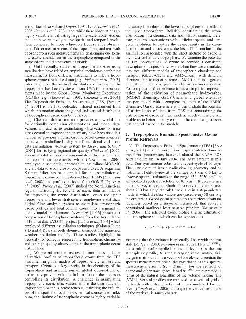
Figure 6. Latitude-altitude cross section, at 75�W on 15 August 2006, of (a) NOx, (b) modeled ozonewithout assimilation, and (c) modeled ozone with assimilation. The top row shows the output from AM2-Chem, while the bottom row shows the fields from GEOS-Chem.


9 of 18

D18307

as suggested by Hudman et al. [2007], may indeed berequired to reconcile the a priori discrepancy between thesimulated ozone in GEOS-Chem and the ozone observa-tions from TES over southeastern North America.[21] Differences in the global source of NOx from light-

ning will contribute to differences in the background ozoneabundances over North America in the two models. Theglobal emissions of NOx from lightning in AM2-Chem isabout 2 TgN/a, whereas in GEOS-Chem it is 4.7 TgN/a. Onthe basis of constraints imposed on GEOS-Chem fromspace-based observations of lightning flash counts, Sauvageet al. [2007] recommended a global lightning source of6 TgN/a. They found that this improved the ozone simula-tion in the model in the tropical upper troposphere bybetween 10% and 45%, but the improvements were highlysensitive to the spatial distribution of the lightning NOx

emissions.

5.2. Vertical Distribution of Ozone

[22] The vertical distribution of ozone throughout thetroposphere reflects a combination of in situ photochemicalproduction of ozone, convective transport of ozone and itsprecursors from the boundary layer, and cross-tropopause

transport of ozone from the stratosphere. The interplay ofthese factors is most apparent over the eastern USA, asshown in Figures 6 and 7. The panels in Figures 6 and 7show the ozone and NOx vertical distribution in the modelsat 75�W as a function of latitude and at 40�N as a functionof longitude, respectively. In both models there are largeabundances of NOx in the boundary layer and lowertroposphere over continental North America. This contrib-utes to the ozone abundance in the middle and uppertroposphere due to strong convection over the southeasternUnited States at this time of year, which lifts ozoneprecursors up from the boundary layer.[23] There is a large discrepancy between the two models

in the abundance of NOx in the upper troposphere, due tothe differences in the lightning NOx emissions. In theGEOS-Chem model this secondary maximum in the NOx

concentrations is centered around 10 km at 35�N and 85�W,while in the AM2-Chem model it is absent. This contributessignificantly to the differences in the ozone distributionbetween the models, particularly between 30� and 40�N. Asshown in Figure 6, assimilation of the TES ozone data doesreduce the discrepancy in ozone between the two models.Cooper et al. [2007], using ozonesonde data, locate the

Figure 7. Longitude-altitude cross section of NOx and ozone at 40�N on 15 August 2006. The plots arearranged as those in Figure 6.


10 of 18

D18307

center of the North American summertime ozone maximumapproximately over Alabama (around 35�N and 85�W),which agrees well with the assimilated model results. Forcomparison, we show in Figure 8 the vertical distribution ofthe modeled ozone obtained from GEOS-Chem withoutNOx emissions from lightning. Without NOx from lightningthe ozone maximum in the upper troposphere over thesoutheastern United States is significantly diminished.[24] It should be noted that in addition to increasing the

ozone abundance in the upper troposphere in AM2-Chem,the assimilation also lowers the position of the modeledozone tropopause. This smoothing of the vertical gradient inozone across the tropopause is due to the course verticalresolution of the TES retrievals and the coarse verticalresolution in the upper troposphere and lower stratosphere(UT/LS) of the version of the AM2-Chem model used here.In contrast, in the GEOS-Chem model, which has greatervertical resolution in the UT/LS (and is more comparable tothe TES retrieval grid), there is less of a change in position

of the ozone tropopause after assimilation of the TES data.The lower position of the tropopause in AM2-Chem (bothbefore and after assimilation) leads to higher values ofstratospheric NOx around 15 km, compared to GEOS-Chem, due to the STARS climatology described previously.These NOx values are distinct from those produced fromlightning emissions and are not expected to contribute toozone production in the upper troposphere.[25] At higher latitudes (poleward of 45� to 50�N), the

differences in the vertical distribution of ozone between themodels are much less. The ozone abundance in the middleand upper troposphere at these latitudes reflects the filamentstretching across Central North America in Figure 4, asso-ciated with an intrusion of air from the stratosphere, andwhich assimilation of TES data enhances in both models.The filament originates in the eastern Pacific and is due todownward transport of ozone from the stratosphere off thecoast of the western United States (Figure 7). In bothmodels this downward transport of ozone is enhanced by

Figure 8. Vertical cross section of NOx and ozone in the GEOS-Chem model without NOx emissionsfrom lightning included in the simulation. Figures 8a and 8b are NOx and ozone, respectively, as afunction of latitude at 75�W. Figures 8c and 8d are NOx and ozone, respectively, as a function oflongitude at 40�N. The simulation is for 15 August 2006, the same as shown in Figures 6 and 7.


11 of 18

D18307

Figure 9. Comparison of individual AM2-Chem and GEOS-Chem ozone profiles to ozonesondeprofiles measured on 15 August 2006. In each plot, the ozonesonde profile is shown by the black line, thecolocated GEOS-Chem profile by the blue lines, and the AM2-Chem profiles by the red lines. In eachplot, the model profile obtained without TES assimilation is indicated by the dashed line, whereas theassimilated profiles are shown by the solid lines.


12 of 18

D18307

assimilation. However, in AM2-Chem, the fold in thetropopause, centered around 120�W, is broadened, com-pared to GEOS-Chem, as a result of the assimilation,potentially reflecting the coarser vertical resolution ofAM2-Chem and the smoothing influence of the TESretrievals. Thompson et al. [2007a, 2007b] report that inthe middle to upper troposphere, especially over northeast-ern North America, layers of ozone from the differentsources mentioned previously interleave with one another,and, despite the coarse vertical resolution, TES may havesome sensitivity to these features.

5.3. Comparison to Ozonesonde Data

[26] To verify the changes introduced by the assimilationto the modeled ozone fields, we compared the assimilatedfields to ozonesonde profiles measured by the INTEXOzonesonde Network Study 2006 (IONS-06) (http://croc.gsfc.nasa.gov/intexb/ions06.html, Thompson et al.[2007a, 2007b]. During August 2006, 418 ozonesondeprofiles were launched from 22 stations across North Amer-ica as summarized in Table 1. Figure 9 shows a comparisonbetween individual AM2-Chem and GEOS-Chem ozoneprofiles and ozonesonde profiles measured at a number ofdifferent locations across North America on 15 August2006. In most cases, the TES assimilation leads to anincrease in ozone in both models throughout the atmo-sphere, which improves the model profile relative to theozonesonde profiles. In some cases, particularly over theeastern North America (Beltsville, Huntsville, Narragansettand Walsingham), the surface emissions in the two modelslead to an overestimate in the ozone abundance in the lowertroposphere which the assimilation cannot correct due tolimited sensitivity of the TES measurements to ozone in theboundary layer. The comparison in the upper troposphereshows, in general, that the assimilated GEOS-Chem profilesare in better agreement with the ozonesonde data, whereas

the assimilated AM2-Chem profile typically overestimatethe ozone abundance (as illustrated, for example, in theprofiles from Beltsville and Walsingham).[27] The mean difference between the models and the

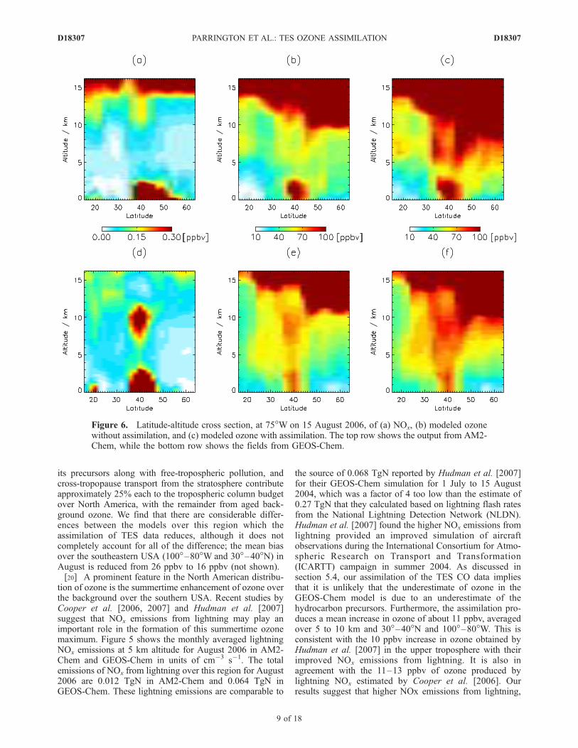
IONS-06 data during August 2006 are shown in Figure 10.Without assimilation the mean difference between the AM2-Chem profiles and the sonde data is large, up to almost�40% in the midtroposphere. Assimilation of TES datareduces this considerably, down to within 10% in themidtroposphere. In the upper troposphere in AM2-Chem,the model profile is greater than the ozonesonde profile byalmost 20% which is further increased following the assim-ilation, to more than 50%, reflecting the coarse verticalresolution in the model over that part of the atmosphere andissues with mapping the AM2-Chem model profiles to theTES retrieval grid (which has a relatively finer verticalresolution) in the assimilation. The mean differences be-tween the GEOS-Chem profiles and the sonde data aresmaller than in AM2-Chem, of order 15-20% in the lower tomidtroposphere and up to 30% at 200 hPa. Followingassimilation of TES data, the mean differences betweenthe GEOS-Chem and ozonesonde profiles are greatly re-duced, to less than 5% throughout the atmosphere up toabout 200 hPa where it increases up to approximately 10%.This is not as great as the change in the AM2-Chem profilesin the upper troposphere, and is well within the variability ofthe ozonesonde profiles. This difference in the response ofthe models to the assimilation in the upper troposphere andlower stratosphere reflects the higher vertical resolution ofGEOS-Chem in this region of the atmosphere.[28] The mean atmospheric state is mostly determined by

large scale processes, such as intercontinental transport, thathave sufficient spatiotemporal scales to be well sampled byTES, giving rise to the improvements in the mean modelprofiles shown in Figure 10. As shown in Figure 9,individual ozonesonde profiles exhibit detailed verticalstructure which is not captured by the models before orafter the assimilation of TES data. This fine vertical struc-ture is due to short spatiotemporal scale processes which themodels are unable to resolve, and TES does not sample theatmosphere with sufficient density to have an impactthrough the assimilation. Therefore we do not expect theTES assimilation to improve the model variability relativeto the ozonesondes. The standard deviation of the meanprofiles is shown in Figures 10c and 10f. Without the TESassimilation, the standard deviation of the two modelprofiles is less than that of the ozonesonde profiles by 20to 50 ppbv throughout the troposphere. Below approximate-ly 300 hPa, the TES assimilation has little impact on thestandard deviation, reflecting the limitations in representingthe small scale atmospheric processes. Above 300 hPa, theassimilation improves the standard deviation relative to theozonesondes, reflecting the increase in ozone lifetime withincreasing altitude which in turn subjects the ozone profileto larger scale processes which are captured by TES.

5.4. Impact of the CO Assimilation on Ozone

[29] Atmospheric CO is a by-product of incompletecombustion and is produced from the oxidation of atmo-spheric hydrocarbons. It is a precursor of troposphericozone and because of its long lifetime it is a useful proxyfor the long-range transport of other ozone precursors from

Table 1. Ozone Sounding Stations Used During the IONS-06

Measurement Campaign in August 2006, and the Number of

Ozonesonde Profiles Involved in Calculating the Mean Sonde

Profiles

Station Name Latitude, �N Longitude, �E Number

Barbados 13.2 �59.5 23Beltsville 39.0 �76.5 12Boulder 40.0 �105.2 31Bratts Lake 50.2 �104.7 29Edmonton 53.6 �114.1 4Egbert 44.2 �79.8 15Holtville 32.8 �115.4 20Houston 29.7 �95.4 16Huntsville 35.3 �86.6 29Kelowna 49.9 �119.4 27Mexico 19.4 �98.6 10Narragansett 41.5 �71.4 28Paradox 43.9 �73.6 5Ron Brown 29.7 �95.4 16Sable 44.0 �60.0 28Socorro 36.4 �106.9 25Table Mountain 34.4 �117.7 31Trinidad Head 40.8 �124.2 30Valparaiso 41.5 �87.0 5Wallops Island 37.9 �75.5 11Walsingham 42.6 �80.6 10Yarmouth 43.9 �66.1 13


13 of 18

D18307

combustion and biogenic sources. To isolate the contribu-tion of the assimilation of CO data to the change introposphere ozone shown in the previous sections, weexamine here the results obtained when only the TES COdata are assimilated.[30] The modeled CO distribution and the changes in CO

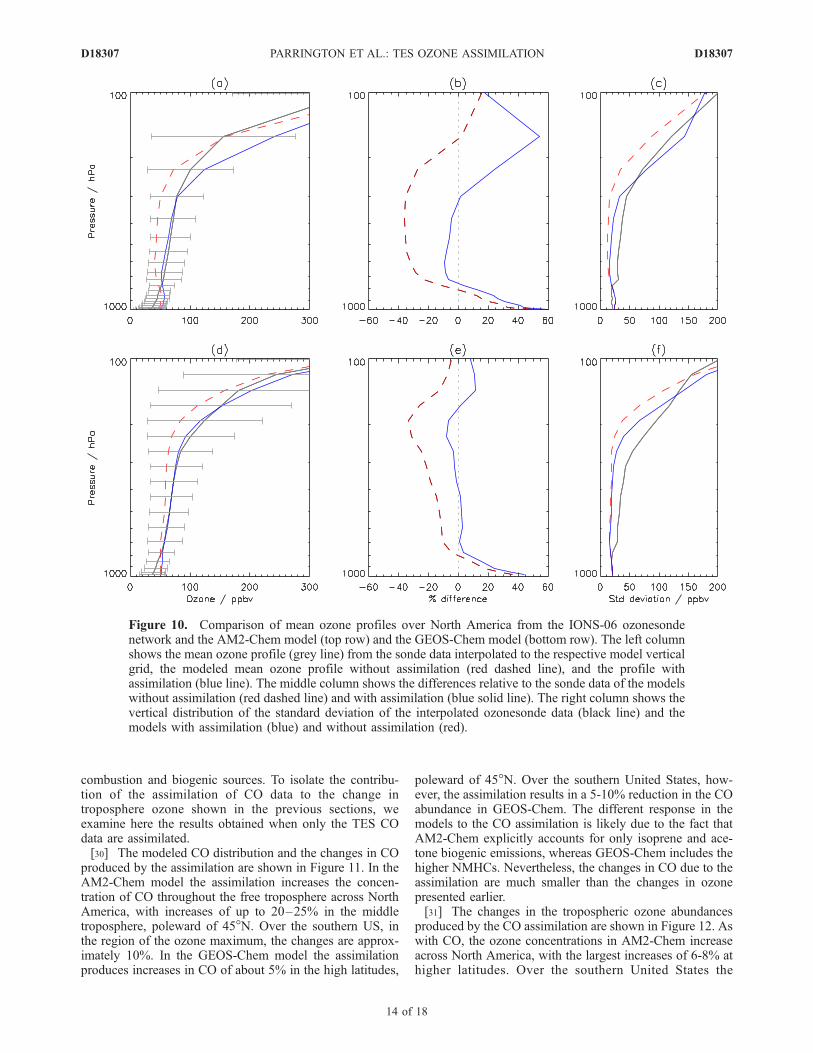
produced by the assimilation are shown in Figure 11. In theAM2-Chem model the assimilation increases the concen-tration of CO throughout the free troposphere across NorthAmerica, with increases of up to 20–25% in the middletroposphere, poleward of 45�N. Over the southern US, inthe region of the ozone maximum, the changes are approx-imately 10%. In the GEOS-Chem model the assimilationproduces increases in CO of about 5% in the high latitudes,

poleward of 45�N. Over the southern United States, how-ever, the assimilation results in a 5-10% reduction in the COabundance in GEOS-Chem. The different response in themodels to the CO assimilation is likely due to the fact thatAM2-Chem explicitly accounts for only isoprene and ace-tone biogenic emissions, whereas GEOS-Chem includes thehigher NMHCs. Nevertheless, the changes in CO due to theassimilation are much smaller than the changes in ozonepresented earlier.[31] The changes in the tropospheric ozone abundances

produced by the CO assimilation are shown in Figure 12. Aswith CO, the ozone concentrations in AM2-Chem increaseacross North America, with the largest increases of 6-8% athigher latitudes. Over the southern United States the

Figure 10. Comparison of mean ozone profiles over North America from the IONS-06 ozonesondenetwork and the AM2-Chem model (top row) and the GEOS-Chem model (bottom row). The left columnshows the mean ozone profile (grey line) from the sonde data interpolated to the respective model verticalgrid, the modeled mean ozone profile without assimilation (red dashed line), and the profile withassimilation (blue line). The middle column shows the differences relative to the sonde data of the modelswithout assimilation (red dashed line) and with assimilation (blue solid line). The right column shows thevertical distribution of the standard deviation of the interpolated ozonesonde data (black line) and themodels with assimilation (blue) and without assimilation (red).


14 of 18

D18307

increases were only 2–6%. In comparison, the increase inozone in AM2-Chem were between 25–50% when both COand ozone observations were assimilated. In GEOS-Chem,which has amore complete treatment of theNMHC oxidationchemistry, the absolute CO-induced changes in ozone aresmall, less than 1%. Over the southern United States theozone concentrations in GEOS-Chem also decrease by less

than 1% as a result of the reduced CO in this region in theassimilation. Li et al. [2005] showed that biogenic emissionsrepresent the dominant contribution to CO over southeasternNorth America in summer. The reduced CO in the GEOS-Chem assimilation suggests that it is unlikely that theunderestimate of ozone in the model in this region, relativeto TES, is due to an underestimate of the hydrocarbon

Figure 11. Monthly mean modeled CO distribution over North America at 5 km for 15 August 2006.The panels are arranged as in Figures 2 and 4.


15 of 18

D18307

precursors of ozone in GEOS-Chem. It implies that theunderestimate of NOx emissions from lightning, as discussedabove, is the likely source of the ozone discrepancy.

6. Conclusions

[32] We have presented a framework for, and the firstresults of, the assimilation of tropospheric ozone profilesretrieved from measurements made by the TES instrument.We used a sequential suboptimal Kalman filter to assimilateobservations of CO and ozone into the AM2-Chem andGEOS-Chem models for July–August 2006. Assimilationof the TES data improves significantly the consistency ofthe ozone distribution between the two models, despitedifferences in the chemical and transport schemes of themodels. For example, the version of AM2-Chem used herehas a more simplified representation of nonmethane hydro-carbon chemistry then GEOS-Chem, and has a globalsource of NOx from lightning of 2 TgN/a compared to4.7 TgN/a in GEOS-Chem. Assimilation of TES datasignificantly increases the ozone abundances in both mod-els. Over North America the assimilation reduces theabsolute mean difference in ozone in the middle troposphere

between the two models from about 8 ppbv to about1.5 ppbv. This reduction in the mean ozone differencebetween the two models demonstrates that the TES datahave sufficient information for constraining the ozonedistribution in the models.[33] The major discrepancy in the ozone simulation over

North America between the two models is in the uppertroposphere over the southeastern United States, where theGEOS-Chem model produces significantly more ozone thanthe AM2-Chem model. The higher abundances of ozone inGEOS-Chem are associated with a secondary maximum inthe abundance of NOx in the upper troposphere, due toemissions of NOx from lightning. In AM2-Chem NOx

emissions from lightning over North America are about afactor of five smaller than in GEOS-Chem and the second-ary maximum in NOx in the upper troposphere over thesoutheastern United States is absent. Assimilation of TESdata enhances ozone abundances in this region in bothmodels. In GEOS-Chem, ozone increases by about 11 ppbvin the upper troposphere, which is consistent with theincrease in upper tropospheric ozone obtained by Hudmanet al. [2007] using GEOS-Chem with an improved lightningNOx source. In AM2-Chem the assimilation increases the

Figure 12. Monthly mean modeled ozone distribution over North America at 5 km for August 2006with only TES CO assimilated (a and b). Figures 12c and 12d show the percentage differences betweenozone from the CO only assimilation to the nonassimilated ozone fields shown in Figures 2a and 2b.


16 of 18

D18307

ozone abundance and reduces the gradient in ozone acrossthe tropopause in the model. In contrast, the change in thegradient in ozone across the tropopause is much less inGEOS-Chem. The change in ozone across the tropopause inAM2-Chem is due to the smoothing influence of the TESretrievals and the coarse vertical of the version of AM2-Chem used in the analysis. Although the assimilation triesto compensate for the bias in ozone in the upper troposphereover the southeastern United States in AM2-Chem, a largeresidual bias in the model clearly indicates the critical needfor correctly representing emissions in the chemistry.[34] Comparison of the assimilated ozone fields with

ozonesonde measurements from the IONS-06 campaign inAugust 2006 show that both models, following assimilationare in better agreement with the sonde data and provide amore accurate description of the vertical distribution ofozone in the troposphere. Over North America the GEOS-Chem model has a mean bias with respect to the ozone-sonde profiles reaching a maximum of -30% at 200 hPa,while the maximum mean bias in AM2-Chem is almost -40% around 500 hPa. Following assimilation, the absolutebias in GEOS-Chem is reduced to less than 5% between800–200 hPa, whereas in AM2-Chem the absolute bias inthe assimilated ozone fields is less than 10% between 800–300 hPa. We found that the assimilation increased signifi-cantly the bias in the AM2-Chem ozone fields, relative tothe sonde data, in the upper troposphere, between 300–100 hPa. As discussed above, this is due to the coarsevertical resolution of the version of the AM2-Chem modelused here. Vertical profiles retrieved from a nadir infraredviewing satellite instrument such as TES will have a coarsevertical resolution, with averaging kernels reflecting thesmoothing of information over a large vertical range. Whenthis is combined with a model with coarse vertical resolu-tion, the assimilation can lead to an overestimate of theozone in the upper troposphere. In GEOS-Chem this is lessof an issue than in AM2-Chem as its vertical resolution ismore comparable to that of TES retrieval grid. This clearlyillustrates the necessity for higher resolution data andmodels in the upper troposphere and lower stratosphere toaccurately reproduce the ozone distribution in this region ofthe atmosphere. Indeed, the resolution issues related toAM2-Chem are expected to be resolved with forthcomingimprovements to the model in AM3, which will have48 levels with a vertical resolution of 1 km in the UT/LS.[35] The dramatic improvement obtained in the compar-

isons between the models and the ozonesonde data afterassimilation demonstrates that TES does indeed providevaluable information on the distribution of troposphericozone and that assimilation of this information into GCMsor CTMs can produce a significantly improved descriptionof ozone abundances in the free troposphere in thesemodels. This will be valuable for a range of applications,such as chemical weather forecasting, estimating the con-tribution from tropospheric ozone to the radiative forcing ofthe climate system, and obtaining a better understanding ofthe underlying chemical processes controlling troposphericozone.

[36] Acknowledgments. This work was supported by funding fromthe Canadian Foundation for Climate and Atmospheric Sciences (CFCAS)and the Natural Sciences and Engineering Research Council (NSERC). The

GEOS-Chem model is maintained at Harvard University with support fromthe NASA Atmospheric Chemistry Modeling and Analysis Program.

ReferencesBeer, R., T. A. Glavich, and D. M. Rider (2001), Tropospheric emissionspectrometer for the Earth Observing System’s Aura satellite, Appl. Opt.,40(15), 2356–2367.

Benkovitz, C. M., M. T. Scholtz, J. Pacyna, L. Tarrason, J. Dignon, E. C.Voldner, P. A. Spiro, J. A. Logan, and T. E. Graedel (1996), Globalgridded inventories of anthropogenic emissions of sulfur and nitrogen,J. Geophys. Res., 101(D22), 29,239–29,253.

Bey, I., et al. (2001), Global modeling of tropospheric chemistry withassimilated meteorology: Model description and evaluation, J. Geophys.Res., 106(D19), 23,073–23,095.

Bowman, K. W., J. Worden, T. Steck, H. M. Worden, S. Clough, and C. D.Rodgers (2002), Capturing time and vertical variability of troposphericozone: A study using TES nadir retrievals, J. Geophys. Res., D23(D23),4723, doi:10.1029/2002JD002150.

Bowman, K. W., et al. (2006), Tropospheric emission spectrometer: Retrie-val method and error analysis, IEEE Trans. Geosci. Remote Sens., 44(5),1297–1307.

Brasseur, G. P., X. Tie, P. J. Rasch, and F. Lefevre (1997), A three-dimen-sional simulation of the Antarctic ozone hole: Impact of anthropogenicchlorine on the lower stratosphere and upper troposphere, J. Geophys.Res., 102(D7), 8909–8930.

Chai, T., et al. (2007), Four-dimensional data assimilation experiments withInternational Consortium for Atmospheric Research on Transport andTransformation ozone measurements, J. Geophys. Res., 112, D12S15,doi:10.1029/2006JD007763.

Clark, H. L., M.-L. Cathala, H. Teyssedre, J.-P. Cammas, and V.-H. Peuch(2006), Cross-tropopause fluxes of ozone using assimilation of MOZAICobservations in a global CTM, Tellus, Ser. A and Ser. B, 59B, 39–49.

Clough, S. A., et al. (2006), Forward model and Jacobians for TroposphericEmission Spectrometer retrievals, IEEE Trans. Geosci. Remote Sens.,44(5), 1308–1323.

Cooper, O. R., et al. (2006), Large upper tropospheric ozone enhancementsabove midlatitude North America during summer: In situ evidence fromthe IONS and MOZAIC ozone measurement network, J. Geophys. Res.,111, D24S05, doi:10.1029/2006JD007306.

Cooper, O. R., et al. (2007), Evidence for a recurring eastern North Amer-ican upper tropospheric ozone maximum during summer, J. Geophys.Res., 112, D23304, doi:10.1029/2007JD008710.

Duncan, B. N., R. V. Martin, A. C. Staudt, R. Yevich, and J. A. Logan(2003), Interannual and seasonal variability of biomass burning emissionsconstrained by satellite observations, J. Geophys. Res., 108(D2), 4100,doi:10.1029/2002JD002378.

Duncan, B. N., J. A. Logan, I. Bey, I. A. Megretskaia, R. M. Yantosca, P. C.Novelli, N. B. Jones, and C. P. Rinsland (2007), Global budget of CO,1988–1997: Source estimates and validation with a global model,J. Geophys. Res., 112, D22301, doi:10.1029/2007JD008459.

Elbern, H., and H. Schmidt (2001), Ozone episode analysis by four-dimensional variational chemistry data assimilation, J. Geophys. Res.,106(D4), 3569–3590.

Fiore, A. M., D. J. Jacob, H. Y. Liu, R. M. Yantosca, T. D. Fairlie, and Q. Li(2003), Variability in surface ozone background over the United States:Implications for air quality policy, J. Geophys. Res., 108(D24), 4787,doi:10.1029/2003JD003855.

Fishman, J., A. E. Wozniak, and J. K. Creilson (2003), Global distributionof tropospheric ozone from satellite measurements using the empiricallycorrected tropospheric ozone residual technique: Identification of theregional aspects of air pollution, Atmos. Chem. Phys., 3, 893–907.

Geer, A. J., et al. (2006), The ASSET intercomparison of ozone analyses:Method and first results, Atmos. Chem. Phys., 6, 5445–5474.

GFDL GAMDT (2003), The new GFDL global atmosphere and land modelAM2-LM2: Evaluation with prescribed SST simulations, J. Clim., 17(24),4641–4673.

Horowitz, L. W. (2006), Past, present and future concentrations of tropo-spheric ozone and aerosols: Methodology, ozone evaluation, and sensitiv-ity to aerosol wet removal, J. Geophys. Res., 111, D22211, doi:10.1029/2005JD006937.

Horowitz, L.W., et al. (2003), A global simulation of tropospheric ozone andrelated tracers: Description and evaluation of MOZART, version 2,J. Geophys. Res., 108(D24), 4784, doi:10.1029/2002JD002853.

Hudman, R. C., et al. (2004), Ozone production in transpacific Asian pollu-tion plumes and implications for ozone air quality in California, J. Geo-phys. Res., 109, D23S10, doi:10.1029/2004JD004974.

Hudman, R. C., et al. (2007), Surface and lightning sources of nitrogenoxides over the United States: Magnitudes, chemical evolution and out-flow, J. Geophys. Res., 112, D12S05, doi:10.1029/2006JD007912.


17 of 18

D18307

Jones, D. B. A., K. W. Bowman, P. I. Palmer, J. R.Worden, D. J. Jacob, R. N.Hoffman, I. Bey, and R. M. Yantosca (2003), Potential of observationsfrom the Tropospheric Emission Spectrometer to constrain continentalsources of carbon monoxide, J. Geophys. Res., 108(D24), 4789,doi:10.1029/2003JD003702.

Jourdain, L., et al. (2007), Tropospheric vertical distribution of tropicalAtlantic ozone observed by TES during the northern African biomassburning season,Geophys. Res. Lett.,34, L04810, doi:10.1029/2006GL028284.

Khattatov, B. V., J.-F. Lamarque, L. V. Lyjak, R. Menard, P. Levelt, X. Tie,G. P. Brasseur, and J. C. Gille (2000), Assimilation of satellite observa-tions of long-lived chemical species in global chemistry transport models,J. Geophys. Res., 105(D23), 29,135–29,144.

Kulawik, S. S., G. Osterman, D. B. A. Jones, and K. W. Bowman (2006),Calculation of altitude-dependent Tikhonov constraints for TES nadirretrievals, IEEE Trans. Geosci. Remote Sens., 44(5), 1334–1342.

Lahoz, W. A., et al. (2007), The Assimilation of Envisat data (ASSET)project, Atmos. Chem. Phys., 7, 1773–1796.

Lamarque, J.-F., B. V. Khattatov, and J. C. Gille (2002), Constrainingtropospheric ozone column through data assimilation, J. Geophys. Res.,107(D22), 4651, doi:10.1029/2001JD001249.

Lawrence, M. G., et al. (2003), Global chemical weather forecasts for fieldcampaign planning: Predictions and observations of large-scale featuresduring MINOS, CONTRACE, and INDOEX, Atmos. Chem. Phys., 3,267–289.

Li, Q., D. J. Jacob, R. J. Park, Y. Wang, C. L. Heald, R. C. Hudman, R. M.Yantosca, R. V. Martin, and M. J. Evans (2005), North American pollu-tion outflow and the trapping of convectively lifted pollution by upper-level anticyclone, J. Geophys. Res., 110, D10301, doi:10.1029/2004JD005039.

Liang, Q., et al. (2007), Summertime influence of Asian pollution in thefree troposphere over North America, J. Geophys. Res., 112, D12S11,doi:10.1029/2006JD007919.

Logan, J. A. (1994), Trends in the vertical distribution of ozone: An ana-lysis of ozonesonde data, J. Geophys. Res., 99(D12), 25,553–25,585.

Logan, J. A. (1999), An analysis of ozonesonde data for the troposphere:Recommendations for testing 3-D models and development of a griddedclimatology for tropospheric ozone, J. Geophys. Res., 104(D13),16,115–16,149.

Luo, M., et al. (2007a), Comparison of carbon monoxide measurements byTES and MOPITT: Influence of a priori data and instrument character-istics on nadir atmospheric species retrievals, J. Geophys. Res., 112,D09303, doi:10.1029/2006JD007663.

Luo, M., et al. (2007b), TES carbon monoxide validation with DACOMaircraft measurements during INTEX-b 2006, J. Geophys. Res., 112,D24S48, doi:10.1029/2007JD008803.

McLinden, C. A., S. C. Olsen, B. Hannegan, O. Wild, and M. J. Prather(2000), Stratospheric ozone in 3-D models: A simple chemistry and thecross-tropopause flux, J. Geophys. Res., 105(D11), 14,653–14,665.

Menard, R., S. E. Cohn, L.-P. Chang, and P. M. Lyster (2000), Assimilationof stratospheric chemical tracer observations using a Kalman Filter. part I:Formulation, Mon. Weather Rev., 128, 2654–2671.

Munro, R., R. Siddans, W. J. Reburn, and B. J. Kerridge (1998), Directmeasurement of tropospheric ozone distributions from space, Nature,392(6672), 168–171.

Nassar, R., et al. (2008), Validation of Tropospheric Emission Spectrometer(TES) nadir ozone profiles using ozonesonde measurements, J. Geophys.Res., 113, D15S17, doi:10.1029/2007JD008819.

Oltmans, S. J., et al. (2006), Long-term changes in tropospheric ozone,Atmos. Environ., 40, 3156–3173.

Osterman, G. B., et al. (2008), Validation of Tropospheric Emission Spec-trometer (TES) measurements of the total, stratospheric and troposphericcolumn abundance of ozone, J. Geophys. Res., 113, D15S16,doi:10.1029/2007JD008801.

Pickering, K. E., Y. Wang, W. Tao, C. Price, and J.-F. Muller (1998),Vertical distributions of lightning NOx for use in regional and globalchemical transport models, J. Geophys. Res., 103(D23), 31,203–31,216.

Pierce, R. B., et al. (2007), Chemical data assimilation estimates of con-tinental U. S. ozone and nitrogen budgets during the IntercontinentalChemical Transport Experiment-North America, J. Geophys. Res., 112,D12S21, doi:10.1029/2006JD007722.

Price, C., and D. Rind (1992), A simple lightning parameterization forcalculating global lightning distributions, J. Geophys. Res., 97(D9),9919–9933.

Price, C., J. Penner, and M. Prather (1997), Nox from lightning: 1. Globaldistribution based on lightning physics, J. Geophys. Res., 102(D5),5929–5941.

Randel, W. J., and F. Wu (1999), A stratospheric ozone trends data set forglobal modeling studies, Geophys. Res. Lett., 26(20), 3089–3092.

Rodgers, C. D. (2000), Inverse Methods for Atmospheric Sounding: Theoryand Practice, World Sci., Hackensack, N. J.

Sauvage, B., R. V. Martin, A. van Donkelaar, X. Liu, K. Chance, L. Jaegle,P. I. Palmer, S. Wu, and T.-M. Fu (2007), Remote sensed and in situconstraints on processes affecting tropical tropospheric ozone, Atmos.Chem. Phys., 7, 815–838.

Segers, A. J., H. J. Eskes, R. J. van der A, R. F. van Oss, and P. F. J. vanVelthoven (2005), Assimilation of GOME ozone profiles and a globalchemistry-transport model, using a Kalman Filter with anisotropic covar-iance, Q. J. R. Meteorol. Soc., 131, 477–502.

Stevenson, D. S., et al. (2006), Multimodel ensemble simulations of pre-sent-day and near-future tropospheric ozone, J. Geophys. Res., 111,D08301, doi:10.1029/2005JD006338.

Tarasick, D. W., V. E. Fioletov, D. I. Wardle, J. B. Kerr, and J. Davies(2005), Changes in the vertical distribution of ozone over Canada fromozonesondes: 1980–2001, J. Geophys. Res., 110, D02304, doi:10.1029/2004JD004643.

Tellmann, S., V. V. Rozanov, M. Weber, and J. P. Burrows (2004), Improve-ments in the tropical ozone profile retrieval from GOME-UV/Vis nadirspectra, Adv. Space Res., 34(4), 739–743.

TES Science Team (2006), TES L2 Data User’s Guide, Jet PropulsionLaboratory, California Institute of Technology, Pasadena, Califor-nia. (Available at http://tes.jpl.nasa.gov/docsLinks/DOCUMENTS/TESL2DataUsersGuidev2.0.pdf)

Thompson, A. M., et al. (2007a), Intercontinental Chemical Transport Ex-periment Ozonesonde Network Study (IONS) 2004: 1. Summertimeupper troposphere/lower stratosphere ozone over northeastern NorthAmerica, J. Geophys. Res., 112, D12S12, doi:10.1029/2006JD007441.

Thompson, A. M., et al. (2007b), Intercontinental Chemical Transport Ex-periment Ozonesonde Network Study (IONS) 2004: 2. Troposphericozone budgets and variability over northeastern North America, J. Geo-phys. Res., 112, D12S13, doi:10.1029/2006JD007670.

Tie, X., S. Madronich, S. Walters, D. P. Edwards, P. Ginoux, N. Mahowald,R. Y. Zhang, C. Lou, and G. P. Brasseur (2005), Assessment of the globalimpact of aerosols on tropospheric oxidants, J. Geophys. Res., 110,D03204, doi:10.1029/2004JD005359.

Wild, O. (2007), Modelling the global tropospheric ozone budget: Explor-ing the variability in current models, Atmos. Chem. Phys., 7, 2643–2660.

Worden, H. M., et al. (2007), Comparisons of Tropospheric Emission Spec-trometer (TES) ozone profiles to ozonesondes: Methods and initial re-sults, J. Geophys. Res., 112, D03309, doi:10.1029/2006JD007258.

Yevich, R., and J. A. Logan (2003), An assessment of biofuel use andburning of agricultural waste in the developing world, Global Biogeo-chem. Cycles, 17(4), 1095, doi:10.1029/2002GB001952.

��K. W. Bowman, Jet Propulsion Laboratory, California Institute of

Technology, MS 183-601, 4800 Oak Grove Drive, Pasadena, CA 91109,USA.L. W. Horowitz, NOAA Geophysical Fluid Dynamics Laboratory, 201

Forrestal Road, Princeton, NJ 08540, USA.D. B. A. Jones and M. Parrington, Department of Physics, University of

Toronto, 60 St. George Street, Toronto, ON, Canada M5S 1A7.([email protected])D. W. Tarasick, Air Quality Research Division, Environment Canada,

Downsview, ON, Canada M3H 5T4.A. M. Thompson, Department of Meteorology, Pennsylvania State

University, 503 Walker Building, University Park, PA 16802-5013, USA.J. C. Witte, Science Systems and Applications Inc., Lanham, MD 20706,

USA.


18 of 18

D18307

estimating the summertime tropospheric ozone distribution ... · 5meteorological services centre,...

Documents