estimating the competitive price of cement from cost … the competitive price of cement from cost...
TRANSCRIPT

1
AGGREGATES, CEMENT AND READY-MIX CONCRETE MARKET INVESTIGATION
Estimating the competitive price of cement from cost and demand data
Summary
1. The purpose of this working paper is to quantify some aspects of the detriment due to
the AECs in cement. In paragraphs 8.271 to 8.273 of the provisional findings, we
provided one estimate of this detriment by reference to our analysis of profitability of
GB cement producers. In this working paper, we seek to estimate the detriment using
another method, namely by comparing the average cement prices and the cement
price that we would expect to observe under effective competition. We refer to this
difference as the overcharge in cement. To do this, we aimed to establish a
benchmark price that would prevail in a well-functioning market and compared that
benchmark price to the actual price of cement. The difference between the
benchmark price and the actual price allowed us to quantify some aspects of the
detriment in cement.
2. To establish our benchmark price, we have derived a competitive supply curve of
cement. The competitive supply curve is derived from producers’ costs of supplying
cement. In a well-functioning market, the interaction of competitive supply and
demand would be expected to establish a market clearing, competitive, price of
cement.
3. We find a benchmark price for 2011 of about £69.50 per tonne, around £10.50 less
than the average price of a tonne of cement in 2011. Based on 8.78 million tonnes of
cement sold in GB in 2011, an overcharge of £10.50 per tonne translates to a
detriment of £92 million in 2011. We will consider the implications of these results for

2
our assessment of proportionality, in the light of any comments we receive, alongside
other estimates of detriment as part of our provisional decision on remedies.
The approach
4. In this working paper our aim is to estimate the overcharge in cement, ie the
difference between the average price of cement in GB cement markets and the price
of cement under effective competition. We aimed to establish a benchmark price that
would prevail in a well-functioning market, and compared that benchmark price to the
actual price. The difference between the benchmark price and the actual price
allowed us to quantify some aspects of the detriment in cement.
5. Coordination may have an impact on any dimension of competition, including price
and output levels, the scope of firms’ geographic operations, investment or
innovation.1 The overcharge measures only the impact on price due to coordination
and thus may not capture the full detriment due to coordination. It does not take into
account losses from any output reduction associated with higher prices.2
6. In our approach to estimating a benchmark price for cement we took existing cement
works’ capacities and costs as given. We used data on capacities and costs to derive
a competitive short-run supply curve of cement. Between them, the supply curve and
the demand for cement will pin down a market clearing price of cement. Since the
supply curve was derived based on the assumption of cement suppliers acting
Neither
does it measure any longer-term or dynamic aspects of detriment, for example due to
reduced investments in efficient production technology or reduced investments in
research and development.
1 The CC’s Guidelines for market investigations (CC3), paragraph 241. 2 When the price is higher than in a well-functioning market, the most price-sensitive customers refrain from buying cement. Some of these customers may have bought more cement at the competitive price. These forgone sales represent a detriment which is not captured by estimates of the overcharge. The detriment due to forgone sales could in principle be estimated if the elasticity of demand for cement in GB were known. Due to the absence of reliable estimates of the elasticity of demand for cement in GB we have chosen not to estimate detriment due to forgone sales. However, the demand for cement is likely to be relatively inelastic, which means the detriment due to forgone sales will be limited.

3
competitively, the market clearing price gives a reasonable indication of what would
constitute a competitive price of cement. The cement overcharge was the difference
between the benchmark price and the actual price.
7. We used data on 2011 costs, capacities and demand to estimate a benchmark price
and compared this with the 2011 weighted average price. Our reasons for using 2011
data were the following:
(a) it is the most recent year for which detailed data on prices, costs and capacities
are available to us; and
(b) after several years of large changes in demand and supply conditions (2008 and
2009), demand and supply conditions stabilized in 2010 and 2011. Indeed, the
demand for cement declined sharply between 2007 and 2009.3 This resulted in
GB cement producers closing or mothballing cement production capacity in 2008
to 2010.4
8. We therefore believe that estimating the detriment based on data on 2011 prices,
costs and capacities is appropriate, though we will take into account more recent
data on total volumes of cement sold in 2012 when this data is available.
In 2011, supply conditions appeared to be stable, and we also note that
demand for cement stabilized in 2010 and 2011.
9. We begin by describing the assumptions we made to derive a competitive supply
curve and the data upon which we based our estimate of the supply curve. We then
describe how we constructed a demand curve and an equilibrium to arrive at a
competitive price.
Deriving a competitive supply curve
10. In order to derive a competitive supply curve we made the following assumptions: 3 See Figure 2.3 in Section 2 of the provisional findings. 4 See Table 11 in Appendix 7.2 of the provisional findings.
4
(a) one-shot outcome, ie no scope for repeated interaction to influence behaviour;
(b) firms are price takers;
(c) one plant’s production decision does not take into consideration its effect on other
plants (ie plants act as if they were all operated by distinct firms, each firm caring
only about its own profit); and
(d) firms do not engage in price discrimination.
11. Assumptions (a) to (c) capture the competitive nature of the market we use to
establish our benchmark competitive price. Assumption (d) simplifies our analysis.
However, we would expect the scope for price discrimination to be limited in a
competitive market, as prices for all customers would tend towards the market
clearing level.
12. The first assumption was made to rule out repeated interaction. If repeated
interaction were considered, there may be scope for coordination. Such outcomes
would not be informative about the competitive price.
13. Assuming firms to be price takers allowed us to identify a competitive outcome.5
14. In addition to assumptions (a) to (d) above, we assumed for the purpose of
exposition that there was no geographic differentiation between cement works. We
Given plants’ fixed and variable costs, we determined whether or not a given plant
would be active at a given price. Since we assumed that firms would not engage in
price discrimination, there was only one price that had to be taken into consideration.
This simplifying assumption enabled us to derive the amount of cement that would be
supplied at a given price.
5 We do this using a tâtonnement process. A tâtonnement process is a process for finding a competitive price. A hypothetical auctioneer announces a price. Each producer states the quantity she would be willing to supply at that price, and each buyer announces the quantity she would be willing to buy at that price. If there is an imbalance between supply and demand, the price is not market clearing and the auctioneer announces a revised price. The process stops when supply and demand balance.

5
maintain that assumption for the purpose of explaining the basics of this approach.
We then relaxed this assumption to allow for a specific type of geographic
differentiation. We describe the approach we took to dealing with geographic
differentiation in the subsection titled ‘Dealing with geographic differentiation’ in
paragraphs 33 to 38.
15. In this analysis, we assume that, absent coordination, cement producers would
behave as price takers and would thus not be able to act strategically or exercise
unilateral market power. In reality, GB cement producers may have a degree of
unilateral market power even in the absence of coordinated behaviour. If this were
the case, the price that would prevail absent coordination may be higher than the
price we estimate here.6
Individual plants’ supply decisions
16. The assumptions (a) to (d) above are in themselves not sufficient to derive a supply
curve for cement. In addition, it was necessary to assess whether or not each
individual plant would be active at a given price, and the volume that active plants
would supply at that price. According to assumption (c) above, each plant decides
independently on whether or not to supply. We note that cement plants are capacity
constrained, and took the view that they will supply when the price of cement
exceeds an appropriate measure of the plant’s costs. This subsection describes how
we reasoned about individual plants’ supply decisions. In particular, it sets out which
costs we considered relevant in these decisions.
6 The assumptions that plants operate independently and that there is no geographic differentiation could also diminish the degree of unilateral market power exhibited by market participants in the model. Since the assumption that firms are price takers already rules unilateral market power out, the assumptions of independence and lack of differentiation are unlikely to make a difference. Only if the assumption of price-taking behaviour were relaxed would the assumptions of independence and lack of differentiation matter in terms of the degree of market power displayed in the model.

6
17. For this analysis, we relied to a large extent on the same data as the analysis in
Appendix 6.5 in the provisional findings. We therefore adopted the same terminology
with respect to costs as in Appendix 6.4:
(a) Distribution costs are the distribution and haulage charges paid by customers for
delivery of the goods from the seller’s sites to the customers’ job sites.7
(b) Variable costs are those costs that necessarily vary in line with small changes in
production volumes (and to a lesser extent, sales volumes) during a normal
production run at an active production site. A key assumption underpinning our
definition of variable costs is that changes in production take place within existing
production capacity limits, such that production could be increased without
necessitating any further investment into plant or equipment. Our definition of
variable costs thus excludes large step-changes in cost associated with
increasing capacity or bringing mothballed capacity back on stream.
Distribution costs do not include the costs of transporting goods or raw materials
between a seller’s sites. The costs of transporting goods or raw material between
a seller’s sites are included in the variable cost, as described below.
(c) Fixed costs are the converse of our definition of variable costs, ie costs that do
not necessarily change in line with production or sales volumes. We subdivided
fixed costs into the following subcategories:
(i) site fixed costs;
(ii) divisional fixed costs;
(iii) central costs; and
(iv) depreciation and amortization.
7 As far as possible, we have used charges paid by customers to cement producers as a proxy for the distribution cost. In the case of Hanson and Tarmac we used actual distribution costs, since these producers did not explicitly charge customers for haulage. We believe delivery charges are a reasonable measure of distribution costs since we do not believe haulage to be a profit centre. If cement producers are in fact making a positive margin on haulage, we would be over-estimating the distribution cost. This, in turn, would lead to an over-estimate of the competitive price and an under-estimate of the overcharge in cement.

7
18. A price-taking firm’s decision about whether to produce at a plant or not depends on
the plant’s costs and the prevailing cement price. In deciding whether to produce or
not, an operator of an existing plant will not take sunk costs into consideration since
these costs have by definition already been incurred or will be incurred regardless of
whether the plant is used for production or not. We considered any central or
divisional fixed costs as being sunk for the purpose of this analysis. If variable costs
and site fixed costs are covered at the prevailing price, there will be a positive
contribution to central or divisional costs. Foregoing this contribution would not be
rational. We also considered depreciation and cost of capital as being sunk for the
purpose of this analysis, since these costs would be incurred regardless of whether
the plant were used for production or not.
19. We defined a plant’s operating costs to include the plant’s site fixed cost, the plant’s
variable cost and the cost of distributing the plant’s output (ie distribution cost). The
operating cost thus excludes divisional and central fixed costs, depreciation and cost
of capital. The operating cost excludes costs which are avoidable only in the long
term and are therefore considered sunk. The operating costs are thus the relevant
costs in deciding whether to use a plant or not in the short term.
20. A plant’s unit operating cost is operating cost divided by output. Unit operating cost
obviously depends on a plant’s output. Unless otherwise stated, our convention has
been to calculate unit operating cost based on a plant’s maximum output, ie when
operating at full capacity. We employ this convention because the unit operating cost
calculated based on a plant’s maximum output is the lowest price at which it could at
all be rational to have the plant in operation.
21. If the market price of cement is too low to even cover a plant’s operating costs (ie
total site cost less depreciation and cost of capital, which are sunk), it will be rational
8
to close or mothball the plant. If the market price is sufficiently high for a plant to
cover its operating costs, it will be rational to operate the plant. This will be the case
even if the price is not high enough to cover the plant’s sunk costs, since those costs
would not decrease even if the plant were to be mothballed.
22. For the purpose of deriving a supply curve, we thus assumed that each plant would
be prepared to supply up to its capacity as long as the price was sufficiently high to
cover the plant’s operating cost.8,9
Demand
23. For the purposes of this analysis, we took the demand for cement as given and equal
to realized GB demand in 2011. This simplified the analysis somewhat and also
reflected the fact that cement demand is likely to be relatively inelastic.10
8 Note that this is not equivalent to a plant always being active when the price is above the plant’s unit operating cost (as calculated based on the plant’s maximum output). It could be that the plant is not in a position to sell more than a fraction of the quantity the plant could produce, in which case the plant would be able to cover its operating cost only if the price were above unit operating cost as calculated based on the plant’s maximum output.
However,
we recognized that this assumption could have implications for our conclusions: a
more elastic demand curve will, in general, contribute to establishing a higher
benchmark price. A higher benchmark price will in turn result in a lower estimate of
detriment due to prices. On the other hand, a more elastic demand curve will mean
that there is a larger detriment arising from higher prices due to lower volumes being
sold as a result of these higher prices (see paragraph 5 above). Therefore, the effect
of a more elastic demand on the overall estimate of detriment is not clear-cut: the
direct price effect is likely to be less, but the effect due to lower volumes being sold
will be higher.
9 For a plant to be able to commit to not selling at any price which covers operating cost, it would need some degree of unilateral market power. This assumption is thus not independent, but rather a consequence of the assumption that firms are price takers. 10 Cement is an intermediate good; it serves as an input to various construction projects, has very few substitutes and the cost of cement represents only a relatively small proportion of the final price of such projects. Therefore, the demand for cement is unlikely to respond much to changes in prices of cement.

9
24. We maintained the assumption of given demand in our analysis, and chose to
discuss the implications of this assumption when assessing our results. Our analysis
of how the conclusions change when demand is more responsive to changes in price
is in Appendix 4.
25. Once we had constructed a demand curve, we calculated the market clearing prices.
This is illustrated in Figure 1. The demand curve is shown as a vertical line in the
figure, and the supply curve is pictured as a sequence of blocks denoted A–D. Each
block corresponds to a production plant. The width of a block represents the
corresponding plant’s capacity and the height of a block represents the
corresponding plant’s unit operating cost. In the figure, it can be seen that the price
would have to be above the unit operating cost of plant C in order for the market to
clear. At any lower price, there would be too little cement to meet demand. It can also
be seen that if the price were to exceed the unit operating cost of plant D, then plant
D would have an incentive to produce and there would be excess supply.

10
FIGURE 1
A supply curve, a demand curve and the marginal plant
Source: CC.
26. We refer to the least efficient plant that has to operate in order to fill demand as the
marginal plant. In the figure, plant C is the marginal plant.
27. Since cement producers’ production capacities are limited, prices can rise above the
marginal plant’s unit operating cost due to customers competing for limited quantities.
On the face of it, such situations appear to be non-competitive in the sense that firms
are selling at prices above marginal or average incremental cost. This would seem at
odds with price competition—usually one would expect there to be an incentive to
gain additional business by under-cutting rivals’ prices. However, this assumes that
firms can expand output without incurring high incremental costs. If all plants are
operating at full capacity, this is clearly not the case. Thus, no plant would have an
incentive to expand its output and thereby depress the market price.

11
28. This shows that the marginal plant’s unit operating cost is only a lower bound on the
market clearing price. If we identify the marginal plant for the GB cement market, we
can use cost data for this plant to estimate a lower bound for the competitive price of
cement.
29. The set of prices that can be supported by a competitive outcome in a given market
configuration is bounded from above by the cost of bringing additional capacity
online.11
30. Additional capacity can be brought online in many ways: de-mothballing of a
mothballed plant, expanding the capacity of an existing plant (eg debottlenecking), or
building a new plant. In addition to this, imported cement or imported clinker ground
in GB could also act as a form of entry. Imported cement is different from other types
of entry as an importers’ capacity does not come in discrete increments to the same
extent as domestic producer’s capacity. Whether the upper bound is given by
imports, de-mothballed capacity or new capacity depends on which the marginal
plant is and which mothballed capacity exists.
In the figure, plant D represents idle capacity which would be brought online
if the price were to rise sufficiently.
31. Since capacity comes in ‘lumps’ and we assumed that demand is given, it will in
general not be possible to have an exact match between demand and supply. If
demand is such that the marginal plant can only sell a small fraction of its potential
output, it would not be economically rational to keep the plant operational unless the
cement price is far above the plants unit operating cost.12
11 This is subject to the caveat in paragraph
If the marginal plant has to
supply a volume close to its capacity in order to satisfy demand, we will use the
22. 12 There is also a more theoretical point related to existence of equilibrium. Unless we assume that plants get to serve customers according to efficiency, ie most efficient plant gets to sell all its output before the second most efficient plant gets to sell etc, it would be the case that all plants that can economically supply at a given price will want to produce at capacity. This would lead to supply and demand not balancing. An assumption that plants get to serve customers in order of efficiency might be unrealistic outside a very structured, auction-like setting. In a structured setting such behaviour might arise in equilibrium.

12
marginal plant’s unit operating cost as an indicator of the lower bound on the
competitive price.
32. Cement imports may be used to fill any gaps between supply and demand if
domestic supply is not well matched to domestic demand. Another alternative would
be for GB suppliers to operate the marginal plant at or close to full capacity and
export any excess cement. Given that GB producers’ exports are very limited, the
latter option seems less plausible. A third possibility is that all plants operate at
slightly lower capacity and the price is slightly above the unit operating cost of the
marginal plant.
Dealing with geographic differentiation
33. The cost of transporting cement represents a meaningful fraction of the price a
customer pays for the product. We therefore considered how best to reflect
differentiation between cement works in terms of geographic location and other
aspects of logistical efficiency in identifying a benchmark price.
34. Figure 2 shows that most cement plants are located in a fairly small geographic area,
with Lafarge’s Dunbar and Aberthaw being exceptions. The latter are located in
southern Scotland and southern Wales, respectively. We have captured this
geographic differentiation by assuming that these plants will sell in their local areas
(Scotland and Wales),13
13 Dunbar sold [] per cent of its output in Scotland in 2011. Aberthaw sold [] per cent of its output to Wales in 2011.
and that any residual capacity at these plants can then be
used to supply England. We have also estimated the cost of supplying cement into
England from these plants.

13
FIGURE 2
Map of the Majors’ cement plants in the UK, 2012
Source: MPA website: http://cement.mineralproducts.org/cement/manufacture/location_of_mpa_members_cement_plants.php.
35. The reason for focusing on the price of supplying cement to England is that England
accounts for about 88 per cent of GB cement consumption. To assess detriment, we

14
compare our estimated benchmark price to a volume weighted average of the GB
cement price.14
36. Effectively, we allocated some capacity at each cement works to Scotland and
Wales. This mainly affected the Aberthaw, Ribblesdale, South Ferriby and Dunbar
cement works. Capacity which had not been allocated to Scotland and Wales could
be used to supply England. We called the capacity which has not been allocated
effective capacity. GB cement works capacities and effective capacities are found in
Appendix 1 of this paper.
37. We were concerned that the distribution cost would not properly reflect the costs
faced by the Dunbar and Aberthaw works when serving customers in areas outside
Scotland and Wales, respectively. For this reason we imputed revised distribution
costs to these plants. Costs and imputed distribution costs are found in Appendix 2 of
this paper.
38. Figures relating to demand for cement and the residual demand (ie demand once
certain quantities have been allocated to Scotland and Wales) are in Appendix 3 of
this paper.
Results
39. Table 1 shows unit operating cost and effective capacity to supply England of all GB
cement works. The cement works have been ranked in ascending order according to
unit operating cost, which means that the most efficient plant appears at the top of
14 Estimating the overcharge by subtracting the benchmark price for England from the GB-wide weighted average is an approximation. A more comprehensive approach would have been to estimate benchmark prices for England, Wales and Scotland, calculate the weighted average of these benchmark prices and then subtract the result from the actual GB-wide average. We have only estimated the price that would prevail in England in a well-functioning market. If the benchmark prices for Scotland and Wales were equal to the benchmark price for England, subtracting the benchmark price for England from the actual GB-wide weighted average does not introduce an error into the overcharge estimate. We note that the gain in precision from following the more comprehensive approach is limited. By way of example, if the benchmark price for England were £70 per tonne and the benchmark prices for Scotland and Wales were £77 per tonne, the error introduced by our approximation is less than £1 per tonne. This is due to the large weight given to England in the weighted average.

15
the table and least efficient plant appears at the bottom of the table. The table also
shows cumulative capacity. For a given cement works, the cumulative capacity is
calculated by summing the effective capacities of all plants which are at least as
efficient as the cement works in question. Comparing the table to Figure 1, the
cumulative capacity on the row of a given plant corresponds to the total capacity of
the plant and of all plants to the left of the plant. Appendix 2 of this paper sets out
how we arrived at unit operating costs and Appendix 1 sets out how we arrived at
effective capacities.
TABLE 1 Unit operating costs and effective capacities to supply England of GB cement works
tonnes/year
Plant Unit operating cost Effective capacity Cumulative effective
capacity
[] [] [] [] [] [] [] [] [] [] [] [] [] [] [] [] [] [] [] [] [] [] [] [] [] [] [] [] [] [] [] [] [] [] [] [] [] [] [] []
Source: GB cement producers’ profit and loss data, GB cement producers’ replies to market questionnaire, CC calculations.
40. We have defined the marginal plant as the least efficient plant that has to be active to
fill demand. The marginal plant is thus found by comparing residual demand to
cumulative effective capacity. We have used a residual demand of 7.7 million tonnes,
see Appendix 3 of this paper. It follows from Table 1 that [Plant 1] is the marginal
plant. [Plant 2] and all plants more efficient than [Plant 2] have an effective capacity
of less than 7.7 million tonnes per year. This means these plants do not have
sufficient effective capacity to fill residual demand and that the market clearing price
must be above £63 per tonne. [Plant 1] and all plants more efficient than [Plant 1]
have a cumulative effective capacity of just over 7.7 million tonnes per year, which is
just sufficient to fill the residual demand of 7.7 million tonnes per year. This implies
that the market clearing price must be at least £66.60 per tonne. If the price were to

16
rise above £69.50 per tonne, [Plant 3] would have an incentive to produce cement.
This would create a situation where there is more supply than there is demand. A
price above £69.50 per tonne would thus not be market clearing. It follows that the
market clearing price is in the range of £66.60 per tonne to £69.50 per tonne, since
the plants that will be supplying cement when the price is in this range have sufficient
capacity to fill demand.
41. The conclusions of our analysis could potentially change if the [] kiln at [Plant 4],
[]. We therefore considered it likely that cement prices would have to increase
significantly to make it rational for [] to [] kiln [].
42. We noted in Appendix 1 that [Plant 5’s] variable cost of serving areas outside []
may in fact be higher than indicated by Table 6. As [Plant 5’s] unit operating cost is
considerably below those of [Plant 1] and [Plant 3], [Plant 5’s] variable cost could rise
considerably before the outcome of our model is affected.
43. We noted above that our assumption of given demand could affect our conclusions.
Appendix 4 of this paper deals with this issue. The analysis in Appendix 4 shows that
a scenario where [Plant 3] is active and the benchmark price is close to £69.50 per
tonne is consistent with a reasonable degree of elasticity of demand. In a scenario
where [Plant 1] is the marginal plant, demand for cement would have to be very
inelastic for supply and demand to balance. We therefore considered this scenario
less plausible.
44. GB producers’ average price of cement in GB was approximately £80 per tonne in
2011.15
15 Volume weighted average of GB cement producers’ price of bulk cement sold to independent buyers in 2011, as found in Table 1 in Appendix 7.8.
A benchmark price of £69.50 per tonne suggests that the overcharge was

17
around £10.50 per tonne in 2011. Based on 8.78 million tonnes of cement sold in GB
in 2011, this translates to a detriment due to elevated prices of £92 million in 2011.16
45. We also note that price of £69.50 per tonne represents the lowest price at which
[Plant 3] would be operating. The plant would be prepared to supply at any price
above £69.50 per tonne. If demand is sufficiently elastic, the competitive price would
be above £69.50 per tonne. As we believe the demand for cement to be inelastic, we
do not believe that the competitive price is materially above £69.50 per tonne.
The role of EU ETS
46. Trading of CO2 allowances could change producers’ incentives to supply cement. If
the ability to trade CO2 allowances gives some plants an incentive to reduce output
in order to sell excess CO2 allowances on the open market, this could affect the price
that would prevail in a well-functioning market.
47. Since we are comparing the 2011 outcome to a 2011 benchmark, we consider EU
ETS Phase II as the relevant framework for assessing the incentives introduced by
emissions trading.17
48. Under EU ETS Phase II, the closing of a plant would mean that the plant’s allocation
of allowances would usually be forfeited.
There was no partial cessation rule in EU ETS Phase II, and
therefore we do not consider it likely that any plant could have an incentive to expand
production due to emissions trading incentives. For this reason, we have restricted
our attention to incentives to reduce output arising from emissions trading.
18
16 We assume here that the £69.50 benchmark price would also apply to Scotland and Wales.
For this reason, we rule out the option of
closing a plant (and thereby avoiding the entire operating cost) and selling all the
17 Please refer to Appendix 2.2 of the provisional findings for a description of the EU ETS emissions trading framework. 18 Cases where the operator of a plant closed an inefficient plant were an exception. In such cases, the operator could transfer the closed plant’s allowances to a more efficient plant.

18
plant’s allowances. In order to be able to sell allowances, a plant would thus have to
incur site fixed cost.
49. A cement works is thus faced with a trade off between producing cement and selling
allowances, and considers site fixed cost as unavoidable when making this choice.
Using the variable and distribution costs in Table 6 and the revised distribution costs
for Aberthaw and Dunbar, the margin between the cement price and variable and
distribution costs is above £14.50 per tonne for all cement works at a cement price of
£69.50 per tonne. The 2011 average price of allowances was about €14 per tonne of
CO2,19 or about £13.50 at the 2011 exchange rate. This suggests that, given the
competitive price of cement of £69.50 per tonne, it would always be more profitable
for GB cement producers to produce cement than to sell allowances. The competitive
price of cement would need to fall to about £68.50 per tonne in order for this not to be
the case, and even if the price were to fall below this point the resulting output
reduction would be very limited.20
Preliminary conclusions
This bound is conservative, since one tonne of
cement corresponds to less than one tonne of CO2. The market price of cement
could therefore drop further before incentives to sell allowances rather than cement
arise. We therefore do not believe that EU ETS affects our estimate of the
competitive price of cement.
50. Based on the above, our preliminary conclusion is that [Plant 3] is likely to be the
marginal plant and that the benchmark price derived from our model is about £69.50
per tonne. This corresponds to a 2011 overcharge of around £10.50 per tonne.
Based on 8.78 million tonnes of cement sold in GB in 2011, an overcharge of £10.50
per tonne translates to a detriment of £92 million in 2011.
19 Provisional findings, Appendix 2.2, Figure 4. 20 []

19
APPENDIX 1
Capacities and effective capacities
1. In this appendix we describe the measures of capacity we have relied on in
estimating the competitive price of cement. We also describe the effective capacities
we calculated to capture geographic differentiation between cement works. The
effective capacity measures a cement works’ capacity to supply England.
Capacity of GB cement works
2. Cement is ground clinker. This means there are two capacity constraints that matter
in the production of cement: kiln capacity and grinding capacity. When ground, one
tonne of clinker will produce approximately 1.1 tonnes of CEM I. We have used the
lesser of 1.1 times a cement works’ clinker capacity and its grinding capacity in our
analysis.
3. We use figures from Appendix 7.2 of the provisional findings for GB cement works’
clinker capacity. These figures take kilns’ planned and unplanned downtime into
account and are thus below kilns’ nameplate capacities.
4. As set out in Appendix 7.2, Lafarge submitted clinker capacities for their cement
works, as well as a measure called ‘expected cement capacity’. They describe this as
‘a synthetic view of what cement is capable of being produced in the ‘context’ of the
constraints for that year’.21
21 Lafarge Tarmac told us that expected cement capacity was affected by factors outside of its control, including market demand, customer specifications, employment and weather, and that these might impact on the ability to produce at ‘expected cement capacity’.
To assess whether Lafarge’s cement works’ capacities
were constrained by clinker capacity or grinding capacity, we divided expected
cement capacity by clinker capacity. If the binding constraint on a cement works is its
clinker capacity, the ratio between expected cement capacity and clinker capacity

20
should be close to 1.1. If the cement works’ output is constrained by some other
factor, the ratio should be significantly below 1.1.
5. The clinker capacity and expected cement capacity of Lafarge’s cement works can
be found in Table 2. This table also contains the ratio between expected cement
capacity and clinker capacity for each cement works. The ratios suggest that
Cauldon and Hope are constrained by their clinker capacities, while Aberthaw and
Dunbar are constrained by other factors. This is consistent with Lafarge’s statement
that Aberthaw is ‘grinding constrained’.
TABLE 2 Lafarge's cement works clinker capacities and expected capacities
Plant Clinker capacity
tonnes/year Expected cement capacity
tonnes/year Expected/
clinker
Aberthaw [] [] [] Cauldon [] [] [] Dunbar [] [] [] Hope [] [] [] Source: Lafarge’s response to the market questionnaire, CC calculations.
6. For our analysis, we thus used expected cement capacity for Aberthaw and Dunbar
as the measure of cement capacity. For Cauldon and Hope, we used 1.1 times
clinker capacity as the measure of cement capacity. Data submitted by Cemex and
Hanson suggest that their cement works are constrained by clinker capacity rather
than grinding capacity.22
Table 3
For these cement works, we used 1.1 times clinker capacity
as a measure of cement capacity. The capacities of GB cement works we used in our
analysis can be found in . Note that with our definition of capacity, these
capacities pertain to CEM I. We have not included mothballed capacity in cement
works’ capacities. The potential for mothballed capacity to alter our conclusions will,
however, be considered in our analysis.
22 Cemex told us that its cement capacity far exceeded its clinker capacity because of Tilbury, a grinding and blending plant.

21
TABLE 3 Capacities of GB cement plants
Plant Capacity
tonnes/year
Rugby [] S Ferriby [] Ketton [] Padeswood [] Ribblesdale [] Aberthaw [] Cauldon [] Dunbar [] Hope [] Tunstead [] Source: GB cement producers’ response to the market questionnaire, CC calculations.
Cement works’ effective capacities to supply England
7. In order to take into account the geographic differentiation between cement works,
we calculated the effective capacity of each GB cement work to supply England. The
effective capacity of a cement works is its remaining capacity once volumes supplied
to Scotland and Wales have been subtracted and measures the cement works’
capacity to supply England.
8. To calculate a cement works’ effective capacity, we subtracted from actual capacity
the volume supplied to Scotland and Wales in 2011 by the works in question. Since
we measured a cement works’ capacity in terms of potential output of CEM I, we
converted any non-CEM-I volumes to CEM I. We assumed that any non-CEM-I
volume was 70 per cent CEM I, for example one tonne of CEM II was converted to
0.7 tonnes of CEM I. The resulting CEM-I-equivalent volumes supplied to Scotland
and Wales by GB cement works are found in Table 4.

22
TABLE 4 Volumes supplied to Scotland and Wales in 2011
tonnes
Plant Scotland Wales
[] [] [] [] [] [] []
[]
[] [] [] [] [] [] [] [] [] [] [] [] [] []
[]
[] [] []
Source: GB cement producers’ transaction data, CC calculations. Note: Volumes have been converted to CEM I equivalent.
9. Cemex’s transaction data did not distinguish between works of manufacture. For this
reason we assumed that any volumes sold by Cemex to customers in Scotland were
manufactured at South Ferriby and any volumes sold by Cemex to customers in
Wales were manufactured at Rugby. This assumption is motivated by the cement
works’ locations and the fact that neither cement works is rail linked.23
10. Table 5
contains GB cement works’ effective capacities. These effective capacities
were obtained by subtracting volumes in Table 4 from the capacities in Table 3.
TABLE 5 GB cement works’ effective capacities
Plant
Effective capacity
tonnes/year
[] [] [] [] [] [] [] [] [] [] [] [] [] [] [] [] [] [] [] []
Source: GB cement producers’ responses to market questionnaire, GB cement producers’ transaction data, CC calculations.
23 While Cemex’s transaction data does not distinguish between works of manufacture, it does distinguish between shipping facilities. The data shows that volumes shipped from the Rugby works to Scotland in 2011 were very limited, which is broadly consistent with our assumption.

23
APPENDIX 2
Costs and revised distribution costs
GB cement works’ operating costs
1. As stated in paragraph 19 above, plant’s operating costs are the relevant costs in
assessing whether or not the plant will be active at a given price. Operating costs
include site fixed cost, plants’ variable costs and plants’ distribution costs, but
excludes depreciation and cost of capital as well as divisional and central costs.
Table 6 shows GB cement works’ operating costs. These figures are based on the
GB cement producers’ profit and loss data.
TABLE 6 Cement works’ 2011 operating costs
Plant Site fixed cost
£ Variable cost
£/tonne Distribution cost
£/tonne
Rugby [] [] [] S Ferriby [] [] [] Ketton [] [] [] Padeswood [] [] [] Ribblesdale [] [] [] Aberthaw [] [] [] Cauldon [] [] [] Dunbar [] [] [] Hope [] [] [] Tunstead [] [] []
Source: GB cement producers’ profit and loss data, CC calculations.
2. The Cauldon, Rugby, Padeswood and South Ferriby plants are not rail linked. This
potentially affects their distribution costs.
3. Note that the operating costs in Table 6 pertain to a cement works’ entire output. The
costs also include the costs of those depots and blending depots that are part of the
delivery networks of the cement plants. To the extent that a cement works produces
CEM II or other blended products, the cost of producing that output is included in the
operating costs. This introduces some imprecision in our analysis as we use the
overall variable cost as one of the components of unit operating cost based on CEM I

24
capacity. We do not think that this approximation introduces any material difference
as most output is CEM I.
Distribution costs
4. Distribution costs are significant in relation to a cement work’s variable costs. The
distribution costs in Table 6 were not well adapted to capturing geographic
differentiation and differentiation terms of logistic efficiency. We only observed
cement works’ distribution costs in aggregate. By dividing a given cement works’ total
distribution cost by its output we got a distribution cost per tonne. Since we did not
control for the typical distance over which a cement works’ output is transported, we
could not arrive at a measure of distribution cost per tonne per mile. It appears
plausible that a cement works primarily serves the customers it is best placed to
serve, and that cement works with less efficient distribution supply over smaller
distances than cement works with more efficient distribution. The observed
distribution cost per tonne would reflect this, and thus not be particularly informative
about a cement works’ location and how efficient a cement works’ distribution is.
5. In particular, the observed distribution cost would not represent a good measure of
the cost faced by a cement works when supplying customers farther afield. The cost
of supplying distant customers is likely important when assessing how the Dunbar
and Aberthaw works affect the competitive price in England. For this reason, we
estimate in the next subsection the costs faced by these plants when supplying
customers in England.
Revised distribution costs for Dunbar and Aberthaw
6. Lafarge’s transaction data contained an estimated haulage cost of shipments. Since
the transaction data distinguishes between regions and identifies a shipments works
of manufacture, the data can be used to estimate the cost of hauling cement from

25
works of manufacture to a given region. We have used 2011 transactions for our
estimates.
7. Lafarge estimated haulage costs in its transaction data. To evaluate the reliability of
these estimates, we compared the volume weighted 2011 average haulage cost per
tonne to the average 2011 distribution cost per tonne as estimated from Lafarge’s
profit and loss data.
8. Table 7 contains Lafarge’s cement works’ haulage costs as estimated from
transaction data and distribution costs as estimated from profit and loss data. Note
that we excluded collected sales when we calculated haulage costs based on
transactions data. We did so on account of collected sales not being informative of
haulage cost.
FIGURE 3
Lafarge’s cement works haulage and distribution costs
[]
Source: Lafarge transaction data, Lafarge profit and loss data, CC calculations.
TABLE 7 Estimated haulage cost and distribution cost per cement works
£/tonne
Works
Estimated cost based on
Transaction data Profit and loss data
Aberthaw [] [] Cauldon [] [] Dunbar [] [] Hope [] [] Source: Lafarge transaction data, Lafarge profit and loss data, CC calculations. Note: We excluded collected sales when calculating the haulage costs from transaction data.
9. Figure 3 shows that the average estimated haulage cost based on the transaction
data is generally below the average distribution cost based on the profit and loss

26
data. For Aberthaw, there is a discrepancy of approximately £[] per tonne. In the
case of Dunbar, there is a discrepancy of around £[] per tonne.
10. Because of the discrepancy between haulage costs (as estimated from transaction
data) and distribution cost (as estimated from profit and loss data), we have decided
not to base our estimates of Aberthaw’s and Dunbar’s costs of supplying England on
the transaction data haulage cost alone. We believe the profit and loss data to be
more reliable as a measure of average distribution cost per tonne. The transaction
data haulage costs appear to be approximated based on radial distances. Since
cement will in practice not be transported in straight lines, this approximation will
underestimate the cost of haulage. However, we believe that the transaction data can
be informative about the relative costs of hauling cement to various regions. To
reconcile these views we rescale the costs of hauling to England in an a manner that
makes the average haulage cost equal to the average distribution cost, as estimated
from the profit and loss data.
Dunbar
11. Table 8 shows estimated haulage costs for the Dunbar works.
TABLE 8 Volume weighted average 2011 haulage costs for destinations inside and outside Scotland
Destination Haulage cost
£/tonne
Scotland [] Other []
Source: Lafarge transaction data. Note: We excluded collected sales when calculating the haulage costs from transaction data.
12. Since there is an economically significant difference in the cost of haulage depending
on whether the destination is in Scotland or not, we believe there is a need to revise
the distribution cost to reflect this.
27
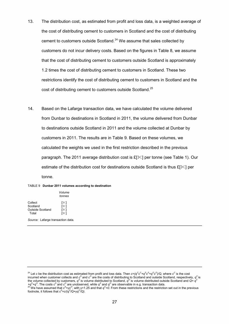
13. The distribution cost, as estimated from profit and loss data, is a weighted average of
the cost of distributing cement to customers in Scotland and the cost of distributing
cement to customers outside Scotland.24
Table 8
We assume that sales collected by
customers do not incur delivery costs. Based on the figures in , we assume
that the cost of distributing cement to customers outside Scotland is approximately
1.2 times the cost of distributing cement to customers in Scotland. These two
restrictions identify the cost of distributing cement to customers in Scotland and the
cost of distributing cement to customers outside Scotland.25
14. Based on the Lafarge transaction data, we have calculated the volume delivered
from Dunbar to destinations in Scotland in 2011, the volume delivered from Dunbar
to destinations outside Scotland in 2011 and the volume collected at Dunbar by
customers in 2011. The results are in
Table 9. Based on these volumes, we
calculated the weights we used in the first restriction described in the previous
paragraph. The 2011 average distribution cost is £[] per tonne (see Table 1). Our
estimate of the distribution cost for destinations outside Scotland is thus £[] per
tonne.
TABLE 9 Dunbar 2011 volumes according to destination
Volume tonnes
Collect [] Scotland [] Outside Scotland [] Total [] Source: Lafarge transaction data.
24 Let c be the distribution cost as estimated from profit and loss data. Then c=(qCcC+qScS+qOcO)/Q, where cC is the cost incurred when customer collects and cS and cO are the costs of distributing to Scotland and outside Scotland, respectively, qC is the volume collected by customers, qS is volume distributed to Scotland, qO is volume distributed outside Scotland and Q= qC +qS+qO. The costs cS and cO are unobserved, while qS and qO are observable in e.g. transaction data. 25 We have assumed that cS=γcO, with γ=1.25 and that qC=0. From these restrictions and the restriction set out in the previous footnote, it follows that cS=c/(qS/Q+γqO/Q).

28
Aberthaw
15. Table 10 shows estimated haulage costs for the Aberthaw works. These are higher
for destinations outside Wales than for destinations in Wales. We believe that the
differences could potentially be economically significant.26
TABLE 10 Volume weighted average 2011 haulage costs for destinations inside and outside Wales
Destintaion Haulage cost
£/tonne
Wales [] Other [] Source: Lafarge transaction data. Note: We excluded collected sales when calculating the haulage costs from transaction data.
16. Since there is an economically significant difference in the cost of haulage depending
on whether the destination is in Wales or not, we believe that there is a need to
revise the distribution cost to reflect this fact. We adjusted the cost in the same way
as we adjusted Dunbar’s distribution cost. Based on the figures in Table 10, we
assume that the cost of distributing cement to customers outside Wales is
approximately 2.2 times the cost of distributing cement to customers in Wales.
17. Based on the Lafarge transaction data, we have calculated the volume delivered
from Aberthaw to destinations in Wales in 2011, the volume delivered from Aberthaw
to destinations outside Wales in 2011 and the volume collected at Aberthaw by
customers in 2011. The results are in Table 11.
Table 11 Aberthaw 2011 volumes according to destination
Volume tonnes
Collect [] Wales [] Outside Wales [] Total [] Source: Lafarge transaction data.
26 Lafarge Tarmac told us that transporting from Aberthaw involved payment of a toll when supplies were transported into England over the Severn Bridge.

29
18. Aberthaw’s 2011 average distribution cost is £[] per tonne (see Table 6). Our
estimate of the distribution cost for destinations outside Wales is thus £[] per
tonne.

30
APPENDIX 3
Demand and residual demand
1. In this appendix, we set out our model of GB demand for cement. In order to capture
the effect of cement works’ locations, we calculate a residual demand. This is the
demand that remains once GB cement works have filled the demand they face in
Scotland and Wales. The appendix has two sections. In the first section, we describe
GB demand. In the second section, we derive the residual demand.
GB cement demand
2. CEM I is the appropriate product to consider in this case, since capacities as set out
in Appendix 1 measure cement works’ capacity to produce CEM I. CEM I is blended
to produce other types of cement. Sales of cement other than CEM I thus indirectly
contribute to demand for CEM I. We assumed that blended cement and bagged
cement contained on average 70 per cent CEM I.27
3. Table 12
contains demand for various types of cement in GB in 2011. Based on the
figures in Table 12 and our assumption that blended cement and bagged cement
contain on average 70 per cent CEM I, we estimated demand for CEM I in GB in
2011 at 8.78 million tonnes. We assumed that unclassified sales are CEM I, on the
grounds that these are sales made by minor importers and our understanding that
most imported cement is CEM I.
TABLE 12 GB 2011 demand for cement
tonnes
Bulk
CEM I Non-CEM-I Bagged Unclassified
6,187,410 1,412,413 1,712,545 409,039
Source: GB cement producers’ and importers’ transaction data, CC calculations.
27 This figure is consistent with MPA data on members’ clinker production and GB cement producers’ transaction data.

31
4. Our estimate of demand for CEM I was not particularly sensitive to changes in the
assumption about the proportion of CEM I in blended cement and bagged cement.
Changing the proportion of CEM I by ten percentage points changed the estimated
demand for CEM I by less than 4 per cent. This was a consequence of most GB
cement sales being sales of CEM I.
5. GB cement works’ total active capacity in 2011 was just over 9.5 million tonnes of
CEM I per year. The available capacity was thus sufficient to meet demand in 2011.
GB cement works meeting GB demand would have required cement works operating
at approximately 92 per cent of full capacity.
Residual cement demand
6. We defined the residual demand as the demand that remains once GB cement works
have filled the demand they face in Scotland and Wales. We calculated the demand
faced in Scotland and Wales in 2011 from Table 4 in Appendix 1 by summing up the
volumes supplied by each cement works in these regions. This gave us an estimated
demand of 1.07 million tonnes, which we subtracted from the GB demand of
8.78 million tonnes to arrive at an estimated residual demand of 7.7 million tonnes.
32
APPENDIX 4
Dealing with elastic demand
1. In our analysis, we assumed that demand for cement was given, ie that customers
would buy the same quantity of cement irrespective of price. While we believe
demand for cement is likely to change only moderately in response to price
changes,28
2. In our analysis, we assumed that the GB demand for cement was equal to the
quantity of cement sold in GB in 2011 and that customers would demand this
quantity irrespective of price. Realized GB demand in 2011 is a point on the demand
curve for cement. We believe the price in 2011 was elevated due to coordination
between GB cement producers and the GGBS arrangements. If demand for cement
is, in fact, somewhat elastic, then demand would be higher at any price below the
2011 price. In particular, demand would be higher at a market clearing price
calculated based on a competitive supply curve and a given demand.
we recognize that assuming that demand is given can affect the
conclusions of our analysis. In this appendix, we evaluate the consequences of this
assumption.
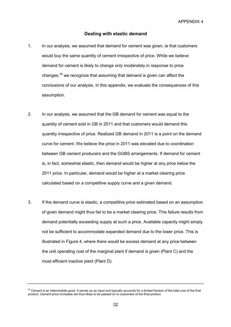
3. If the demand curve is elastic, a competitive price estimated based on an assumption
of given demand might thus fail to be a market clearing price. This failure results from
demand potentially exceeding supply at such a price. Available capacity might simply
not be sufficient to accommodate expanded demand due to the lower price. This is
illustrated in Figure 4, where there would be excess demand at any price between
the unit operating cost of the marginal plant if demand is given (Plant C) and the
most efficient inactive plant (Plant D).
28 Cement is an intermediate good. It serves as an input and typically accounts for a limited fraction of the total cost of the final product. Cement price increases are thus likely to be passed on to customers of the final product.

33
FIGURE 4
Demand at decreased price depending on elasticity of demand
Source: CC.
4. We note that while elastic demand means that the benchmark price will increase, it
does not follow that total detriment will necessarily decrease as a consequence. This
is apparent from inspection of Figure 4. When demand is responsive to price, any
price below the coordinated price implies increased demand. Sales forgone due to
the elevated price represent a source of detriment. If demand were actually elastic,
plant D would be the marginal plant. The detriment due to forgone sales is
represented by triangle between the vertical, assumed demand curve, the actual
demand curve and the line representing the unit operating cost of plant D. If demand
were responsive to price, this detriment would be non-zero. There are thus two
opposing effects at work and the effect on total detriment is therefore not clear-cut. In
particular, it is not obvious that the assumption of given demand would result in an
overestimate of total detriment.

34
5. While we did not have access to an estimate of how elastic the GB demand for
cement is, we could derive an upper bound on how elastic demand can be and still
accommodate an expansion in demand due to a lower price. If the demand for
cement would have to be unreasonably inelastic for the market to balance at our
estimated competitive price, we would have less confidence in the validity of our
estimate.
6. We calculated bounds on the elasticity for demand in two scenarios:
(a) a scenario where [Plant 1] is active but [Plant 3] is not; and
(b) a scenario where [Plant 3] is active.
7. Throughout the analysis, we assumed that the coordinated price was £80 per tonne.
Our analysis relied on the observation that in any scenario, demand could expand by
at most a quantity equal to available spare capacity (measured relative to 2011
demand) before balance of supply and demand is violated.
8. In the first scenario, the competitive price is between £66.60 per tonne and £69.50
per tonne. These prices correspond to reductions of 16 and 13 per cent relative to
the coordinated price, respectively. There would be virtually no available spare
capacity at any price below £69.50 per tonne. Demand would need to be very
inelastic for supply and demand to balance.29
9. In the second scenario, the competitive price is £69.50 per tonne or above. A price of
£69.50 per tonne represents a reduction of 13 per cent relative to the average price
of cement in 2011. With both [Plant 1] and [Plant 3] active spare capacity would be
around []kT per year. In this scenario, demand could thus expand by just under
29 Our estimated of the elasticity of demand was the negative of the relative change in demand divided by the relative change in price. This is equivalent to assuming that the demand curve is linear. Compared with the elasticites implied by a constant elasticity of demand system, the approximation results in slightly more elastic demand.

35
4 per cent relative to realized 2011 GB demand before demand exceeds supply. To a
first approximation, demand price elasticity would, in absolute terms, have to be 0.3
or less for supply and demand to balance at the competitive price.