Estimating the Adverse Selection and Fixed Costs of Trading in Markets

With Multiple Informed Traders

Sugato ChakravartyPurdue University

West Lafayette, IN 47906email: sugato@purdue.edu

Asani SarkarFederal Reserve Bank of New York

New York, NY 10045email: asani.sarkar@frbny.sprint.com

Lifan WuCalifornia State University, Los Angeles

Los Angeles, CA 90032

First Version: April 1997Revised: May 1, 1998

Acknowledgment: The views expressed in the paper are those of the authors’ and do not represent thoseof the Federal Reserve Bank of New York or the Federal Reserve System. We thank AvanidharSubrahmanyam (Subra) for comments on an earlier draft and Marta S. Foth for typing the manuscript. Asalways, we alone are responsible for any errors.

Estimating the Adverse Selection and Fixed Costs of Trading in Markets

With Multiple Informed Traders

Abstract

JEL classification number: G12

We investigate, both theoretically and empirically, the relation between the adverse selection and fixed

costs of trading and the number of informed traders in a financial asset. As a proxy for informed traders,

we use dual traders -- i.e., futures floor traders who execute trades both for their own and customers'

accounts on the same day. Our theoretical model shows that dual traders optimally mimic the size and

direction of their informed customers' trades. Further, the adverse selection (fixed) costs of trading: (1)

decrease (increase) with the number of dual traders m, if dual traders are risk neutral; and (2) are a single-

peaked (U-shaped) function of m, if dual traders are risk averse.

Using data from four selected futures contracts, we find that the number of dual traders are a significant

determinant of both the adverse selection and fixed costs of trading, after controlling for the effects of

other determinants of market liquidity. In addition, for three of the four contracts, the estimated (fixed)

costs of trading are a single-peaked (U-shaped) function of m. The implication from our theory is that the

dual traders in these contracts exhibit risk averse behavior.

1

1. Introduction

An important paradigm in financial markets, originating from Bagehot (1971), is that informed

trading imposes significant adverse selection costs on investors. Copeland and Galai (1983), Glosten and

Milgrom (1985), Kyle (1985), and Admati and Pfleiderer (1988) have all formally modeled Bagehot's

ideas. Several papers have estimated the adverse selection costs empirically (namely, Glosten and Harris

(1988), Madhavan and Smidt (1991) and Hasbrouck (1991). Since informed trading is unobservable,

other papers have sought to identify the cross-sectional determinants of the adverse selection costs. For

example, Brennan and Subrahmanyam (1995) report an empirical relationship between the number of

analysts following a stock and the price per unit of order flow, known as the Kyle-lambda or, simply, λ.

A recent, and important, extension of this literature is Brennan and Subrahmanyam (1998), who

develop a model of a single representative investor who faces both an adverse selection (or, variable) cost

of trading as well as a fixed component. Brennan and Subrahmanyam use the model to derive

comparative statics of the investor’s expected trade size with respect to the variable and fixed costs of

trading. Using data on a large sample of stocks, the authors find that the average trade size is strongly

negatively related to the estimated fixed costs of trading per share.

Our paper contributes to this literature in three way s. One, we identify, both theoretically and

empirically, a distinct group of futures floor traders as informed traders. Two, we estimate the empirical

relationship between the adverse selection costs of trading and the number of informed traders for the

futures contracts in our sample. And three, we establish a new theoretical result on the relationship

between the fixed costs of trading and the number of informed traders, and validate this result empirically.

In futures exchanges, the futures floor tr aders we identify as potentially informed traders are

known as dual traders because they trade both for customers and their own accounts on the same day. 1

The extant theoretical literature argues that dual traders are informed traders. For example, in Fishman

and Longstaff (1992), dual traders are better informed than market makers in determining whether

2

customers are trading for informational reasons. 2 Dual traders’ optimal strategy is to trade in the same

direction as (or piggyback) on their informed customers. In Chakravarty (1994) and Sarkar (1995), dual

traders observe the order size of their customers to infer the information content of these orders. In

equilibrium, dual traders piggyback on informed trades, mimicking both the direction and size of

informed trades.

Our model departs from the existing dual trading literature in using a two-period setting with

variable order size and, further, in allowing risk-aversion on the part of dual traders. 3 The assumption that

dual traders are risk-averse is justified on empirical grounds since many futures floor traders, including

dual traders, trade infrequently and in small amounts (see, for example, Locke, Sarkar and Wu (1998)).

Consistent with the earlier literature, we find that dual traders mimic both the direction and size of

informed trades, although the extent of piggybacking is less due to dual traders’ risk-aversion.

We find that, consistent with Subrahmanyam (1991), the adverse selection cost λ is a single-

peaked function of the number of dual traders m if dual traders are risk-averse. 4 If dual traders are risk-

neutral, then λ is strictly decreasing in m. The intuition for this result is that, for small values of m, λ

increases with m because risk-averse dual traders trade less than they would if they were risk-neutral. For

large values of m, dual traders trade more aggressively as the aggregate risk tolerance of dual traders is

high and, so, λ decreases with m.

A new result is the relationship between the fixed costs of trading and m. Following Brennan

and Subrahmanyam (1998), we assume that the market maker offers an exogenously determined price,

which is linear except for the fixed element. The change in the fixed costs with respect to m is obtained

1 Dual traders are present in all major securities exchanges around the world, such as the stock markets, futuresmarkets, currency and interest swap markets and fixed income markets.2 Fishman and Longstaff (1992) also provide empirical evidence that dual traders’ revenues are higher on days whenthey are also trading for customers, which is consistent with the idea that dual traders personal trades are based oninformation derived from their customer trades. However, Chang and Locke (1992) do not find that dual tradershave profitable private information.3 Fishman and Longstaff (1992) have a two period model with fixed order size while Roell (1990), Chakravarty(1994) and Sarkar (1995) use a single period setting with variable order size. All assume risk-neutrality of informedtrader(s) and broker(s).

3

by deriving the effect of m and the fixed costs, separately, on the dual traders’ expected trade size.

Suppose dual traders are risk-neutral. An increase in m increases market depth (the inverse of λ) and,

consequently, dual traders’ expected trade size. An increase in the fixed costs decreases the expected

trade size, as in Brennan and Subrahmanyam (1998). We show that, as a result of these two effects, the

fixed costs of trading increase with m when dual traders are risk-neutral.

If dual traders are risk-averse, then, for small values of m, an increase in m reduces the market

depth and, consequently, the broker’s expected trade size while an increase in the fixed costs reduces the

trade size, as before. In this case, we show that for small values of m, the fixed costs of trading decrease

with m. For large values of m, the fixed costs of trading increase with m, as in the risk-neutral case.

Hence, the relationship between the fixed costs of trading and m is the reverse of that between the adverse

selection costs of trading and m.

To test the predictions of our model, we empirically examine four futures contracts using the

Computer Trade Reconstruction (CTR) data, which consists of detailed records of every transaction on

the exchange floor. In addition to transaction prices and quantities, the data distinguishes between

purchases and sales and allows us to identify trades executed on behalf of dual traders’ outside customers

and trades executed for dual traders’ personal accounts. We study four futures contracts (Treasure Bond

and soybean oil futures on the Chicago Board of Trade (CBOT); the 91-day Treasury Bill and live hog

futures on the Chicago Mercantile Exchange (CME)), chosen for the diverse range of trading activity they

represent.

We use the Glosten and Harris (1988) and the Madhavan and Smidt (1991) methods to estimate

the fixed and variable costs of trading the four futures contracts. Since m and the estimated trading costs

may be determined simultaneously, we rely on a two-stage least squares, or 2SLS, approach where we

include m2 (m-squared) and the number of locals (floor traders who trade exclusively for their own

accounts) as endogenous variables, in addition to m and the estimated trading costs. The variable m2

4 Subrahmanyam (1991) shows a similar result in a model with risk averse informed traders in a single-periodsetting.

4

enables us to test for non- monotonicity in the m-λ relationship. Since locals often act as if they are

market makers, including the number of locals as an endogenous variable allows us to isolate the effect of

dual trading on market liquidity. Our exogenous variables include customer trading volume, the number

of customer trades, the daily closing price, the price variance, and the open interest. 5

The results are mostly consistent with our model’s predictions and robust with respect to the

method used for estimating trading costs (i.e., Glosten and Harris (1988) or Madhavan and Smidt (1991)).

For all four contracts, the number of dual traders m is a significant determinant of the adverse selection

costs of trading. Further, for three of the four contracts, the estimated adverse selection costs are

increasing in m for small values of m and decreasing in m for relative large values of m. For the

remaining contract, the T-Bond futures, λ decreases with m for relatively smaller values of m, and

increases with m for relatively larger values of m.

For all four contracts, the number of dual traders, m, is also a significant determinant of the fixed

costs of trading. For three of the four contracts, the fixed costs initially decrease in m and then increase.

For the remaining contract, T-Bond futures, the fixed costs initially increase in m and then decrease.

Summarizing, for three of our contracts, T-Bills, soybean oil and live hogs, the estimated

relationship between m and both the adverse selection and fixed costs is consistent with risk aversion of

dual traders. For the remaining contract, T-Bonds, the results are consistent with risk taking by dual

traders. The T-Bond futures pit is ten times more active than any of the other contracts and we conjecture

that active dual traders in that pit are well capitalized and, consequently, are likely to be either risk neutral

or risk takers.

The remainder of the paper is organized as follows. We describe and solve our theoretical model

in section two. Section three discusses the data. In section four, we estimate trading costs using the

Glosten and Harris (1988) method. The empirical relationship between λ and m is examined in section

five, and between the fixed costs of trading and m in section six. In section seven, we repeat our analyses

after estimating trading costs using the Madhavan and Smidt (1991) method. Section eight concludes.

5 The open interest is the daily number of contracts for which delivery is obligated.

5

2. A Dynamic Model of Competitive Dual Trading

A. Structure and Notation

Exchange regulation allows dual traders to act as agents on behalf of their client and as principals

for their personal trade, but not in the same transaction. Further, dual traders are not allowed to trade

ahead of their customers. Consistent with exchange regulations, the dual traders in our model act as

agents for the informed trader in the first period and trade as principals in the second period.

We consider a two-period market for a single risky asset along the lines of Kyle (1985). The

players in the model are: one risk neutral informed trader, m risk averse dual traders each with a negative

exponential utility function and risk-aversion parameter R, a continuum of noise traders who appear in

each of the two trading dates, and a market maker who sees aggregate orders in each period and prices

competitively.

There is a single risky asset with rando m value ~v drawn from a Normal distribution with mean 0

and variance Σ v . A continuum of noise traders submits aggregate order flow ~u1

in period one and ~u2 in

period two, where ~ui is distributed N iu( , ) ,0 1 2Σ ∀ = . All random variables are assumed to be

independent of one another.

We now turn to a formal description of the sequence of events.

B. Sequence of Events

A single (risk neutral) informed trader receives a perfect signal ~v v= about the true asset value

and chooses to trade a quantity x through m risk averse dual traders in the market. We assume that the

informed trader divides his order equally among the dual traders. The dual traders, acting as agents,

submit the informed trader’s order to the market maker for execution. The first period noise trade u1 is

realized and the market maker clears the market at price p1 conditional on observing the net order flow

y x u1 1= + .

6

In the second period, each risk averse broker, acting as a principal, chooses his personal trading

quantity z and submits it to the market maker for execution. Each broker's choice is based on observing

his portion of the order received from the informed trader , x/m and the first period market clearing

price p1 . The second period noise trade u2 is realized and the market maker clears the market at price

p2 , conditional on the net second period order flow y mz u2 2= + , as well as the (realized) first period

market clearing price. Finally, the liquidation value v is publicly observed and both the informed trader

and the dual traders realize their respective profits (if any).

C. Results

Period 1: Only the informed trader's trades are executed in the first period by the m risk-averse dual

traders. Thus, the period one solution is identical to the Kyle (1985) single-period model. Accordingly,

the informed trading quantity x is:

xv=

2 1λ(1)

and the market maker's period 1 price sensitivity parameter is:

λ112

= ΣΣ

v

u

(2)

Period 2: The dual traders trade for their personal accounts in period two having observed x and the first

period market clearing price p1 . Suppose p p y2 1 2 2= + λ . Then, the profit function for broker j,

∀ j=1,2,… ,m is:

Π j j j j j jz v z z u z p z= − + + −−λ2 2 1d i (3)

where z j is the personal trading quantity of the jth broker and z j− is the sum of the trading quantities of

the (m-1) dual traders excluding the jth broker. Each risk averse broker's objective function is defined as:

E x pR

Var x pj jΠ Π, ,1 12d i d i− (4)

7

Broker j maximizes (4) with respect to z j . The following lemma provides a solution for z j .

Lemma 1: For a given λ2 , each broker j's optimal trading quantity for j=1,… ..,m, is:

zx uDj λ λ

21 1b g b g= −

(5)

where,

D m R u= + +λ λ2 221b g b g Σ (6)

Proof: See Appendix A.

From (5) and (6), if R = 0, z j is decreasing in λ2 , which is the usual case. But if R > 0 , z j is

smaller than that in the risk-neutral case for a given λ2 , and by an amount which depends on R and Σ u .

From the market maker's zero profit condition,

λ22

2

= Cov v yVar y

,b gb g (7)

where y mz uj2 2= + .

Lemma 2:

• If R=0, then

λ21

1 2=

+ mm v

u

ΣΣ

(8)

• If R > 0, then λ2 satisfies the fourth-order polynomial

λ2 2 22=

+mD

m Dv

v u

ΣΣ Σ

(9)

where D is defined by (6).

Proof: See Appendix A.

8

Part 1 of lemma 2 implies th at if R = 0, λ2 is decreasing in m. The comparative statics associated

with λ2 for the risk-averse case is presented in proposition 1. But, first, we show that the fourth order

polynomial given by (9) has a unique, real and positive solution.

Lemma 3: There exists a unique, real and positive root of λ2 .

Proof: See Appendix A.

The following proposition captures the relationship between λ2 and m.

Proposition 1:

• If R > 0, then λ2 is a single-peaked function of m.

• If R = 0, then λ2 is monontonically decreasing in m

Proof: See Appendix A.

Proposition 1 states that when R > 0 and the number of risk averse dual traders, m, is below a

critical m* , λ2 increases for increasing values of m. When R > 0 and m is above the critical m* ,

λ2 decreases for increasing values of m. This non-monotonic result, first shown in Subrahmanyam

(1991), follows from the fact that the dual traders' personal trades are informationally motivated. As the

number of dual traders, m, increases, λ2 initially increases due to the fact that these risk-averse dual

traders trade less aggressively than if they were risk neutral. With more dual traders, however, the

aggregate risk tolerance of the dual traders now increases and the dual traders start trading more

aggressively, resulting in more information being revealed in prices and a corresponding decrease in λ2 .

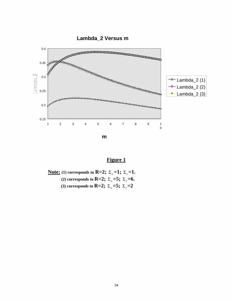
Figure 1 graphically illustrates the non- monotonicity result between λ2 and m for a variety of

values of R, Σ u and Σ v . Specifically, we plot three graphs corresponding to (1) R=2, Σ u =1and Σ v =1;

(2) R=2; Σ u =5; Σ v =6; and (3) R=2; Σ u =5; Σ v =2. The non- monotonity is clearly evident in all three

cases, with the turning points being (approximately) at m*= 2, m* = 5 and m* = 4, respectively.

We now turn to incorporating fixed costs in our model.

9

D. Fixed Costs

As discussed in Brennan and Subrahmanyam (1998), the reality of price discret eness in asset

markets combined with related institutional factors introduce a fixed element to trading costs independent

of trade size. Empirical models that decompose trading costs into fixed order processing costs and the

variable adverse selection costs (for example, Glosten and Harris (1988) and Madhavan and Smidt

(1991)) recognize this fact explicitly. Moreover, recent research, such as George, Kaul and Nimalendran

(1991), conclude that the fixed cost of trading forms the bulk of the trading costs. Therefore, in this

section, we investigate the relationship between the fixed cost of trading and the number of dual traders m

in the market.

The fixed costs per share creates a “no-trade” region in the joint distribution of dual traders’

endowment shocks and signal realizations (i.e., realizations of the informed trade x in period one). Dual

traders will not trade in this region, which is centered at the origin. Since the dual traders’ trades are not

normally distributed, a linear pricing rule is no longer optimal for the market maker.

Instead of endogenizing λ2 , we follow Brennan and Subrahmanyam (1998) and assume that the

market maker in period two offers an exogenously determined price, which is linear except for the fixed

element given by

p Sign y p yf2 2 1 2 2= + +ψ λb g (10)

Notice that in the price specification (10), the second and third terms in the right hand side correspond to

a linear specification while the first term is the fixed element.

If there are fixed costs per share in period one, then the informed trader also faces a no-trade zone

in period one and λ1 is no longer determined from a linear pricing rule. However, our focus is on the

relationship between the fixed costs and m. Since λ1 is independent of m, we simplify and assume that

there are no fixed costs in period one. Thus, x and λ1 are still given by (1) and (2). This assumption

maintains the tractability of our model.

Let us now denote:

10

~ ~ ~r x u= −λ1 1b gThen, without fixed costs, from (5) we can write

~~

zrD

= (11)

where, D is defined by (6). With fixed costs, each broker's equilibrium period-two trade is given by:

zr sign y

Dif r

f =−R

S|T|

~ ψ ψ2b g>

0 otherwise (12)

The following proposition now identifies the nature of the relationship between the fixed cost of

trade and m.

Proposition 2:

• If R > 0, then ψ is a U-shaped function of m, decreasing (increasing) with m for small (large) values

of m.

• If R = 0, then ψ is monotonically increasing in m.

Proof: See Appendix A.

Proposition 2 states that the relationship between m and the fixed cost of trading is the opposite of that

between m the (variable) adverse selection cost of trading. The intuition for the above result follows from

the effect of ψ and m on the broker's expected personal trade size. As in Brennan and Subrahmanyam

(1998), an increase in ψ reduces the broker's expected personal trade size. When R = 0, an increase in m

reduces λand so increases the expected personal trade size. Then, as shown in the appendix, m and

ψ are positively related.

When R > 0, an increase in m increases λfor small values of m and, consequently, ψ and m are

negatively related. For relatively larger values of m, the aggregate risk tolerance of the dual traders

11

increases and so does their expected personal trade size. Thus, in this region, m and ψ are again

positively related.

We now test our theoretical results empirically.

3. Data

The sample period covers thirty randomly selected trading days over the six-month time period

starting August 1, 1990 for the following futures contracts : T-bond futures and soybean oil futures trading on

the Chicago Board of Trade (CBOT); the 91-day T-bill futures and the live hog futures trading on the

Chicago Mercantile Exchange (CME). 6 We use the futures contracts closest to expiration, since these are the

most actively traded. The contracts represent a range of trading activities. The T-bond futures is the most

active futures contract in the United States with an average daily customer trading volume of 119,598

contracts. The three remaining contracts, the live hog, soybean oil and the 91-day T-Bill futures are

intermediate in activity with average daily customer trading volumes of 6,432 contracts, 7,504 contracts and

7,722 contracts, respectively.

The data, known as the Computerized Trade Reconstruction (CTR) data, provides the trade time,

price, quantity, and an identification for the floor trader executing the trade. Unique to this data, the record

indicates whether the trade was a buy or a sell and a customer type indicator (CTI), labeled 1 through 4. For

our purposes, the most important CTI types are 1 (a trade for a floor trader’s personal account) and 4 (a trade

for an outside customer). 7

To identify dual traders and locals, we first calcul ate a trading ratio for each floor trader for each day

she is active. Thus, we define d as the ratio of a floor trader's personal trading volume to his total trading

volume on a day, i.e.,

6 Our choice of sample period and contracts is determined by the availability of data, which is the property of theCommodity Futures Trading Commission (CFTC).7 The other indicators are CTI 2 (trades executed for a clearing member’s house account) and CTI 3 (trades foranother member present on the exchange floor). See Manaster and Mann (1996) for a description of how the CTRdata is put together. Fishman and Longstaff (1992) also use the same data for their study of dual trading.

12

dpersonal trading volume

personal trading volume customer trading volume=

+(13)

For a particular day, we categorize a floor-trader as a dual trader if d lies on the closed interval [0.02, 0.98]. 8

A floor trader is a local on a particular day if d lies on the interval (0.98, 1] for that day.

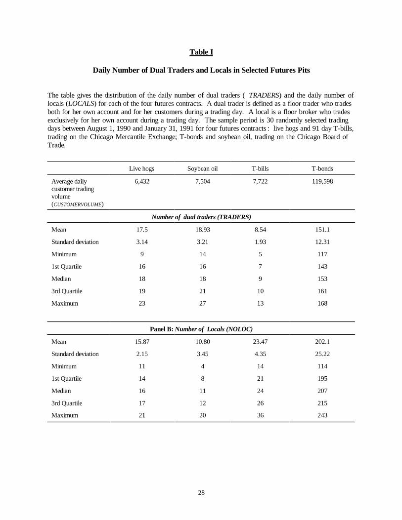
Table I reports the daily distribution of the number of dual traders and loca ls in each of the four

futures contracts. As panel A indicates, the average number of dual traders on a day varies substantially

across the four contracts, ranging from 8.54 for T-bills to 151 for T-bonds. Panel B of table II reports the

daily distribution of locals in the sample. The average number of locals varies from 10.8 in Soybean futures

to 202.1 in T-bond futures.

We now turn to the estimation of the adverse selection and the fixed cost components of customer

trades in each of the four contracts, using the method of Glosten and Harris (1988). Later, we confirm the

robustness of the results by repeating our analysis using the Madhavan-Smidt (1991) method for estimating

the components of the bid-ask spread.

4. Estimation of Adverse Selection and Fixed Costs of Trading

We estimate the adverse selection and fixed costs of trading for customers, using the technique

developed by Glosten and Harris (1988). To do so, we estimate the following regression:

∆p q Q Qt GH t GH t t t= + − +−λ ψ ε1 (14)

where ∆p p pt t t= − − 1 is the price change between the tth and (t-1)th transaction, qt is the (signed) order

flow at time t and Qt is the sign of the incoming order at time t (+1 for a buyer-initiated trade and -1 for a

seller-initiated trade). λGH measures the adverse selection component in a customer trade of size q, while

8The 2% filter is used to allow for the possibility of error trading. As Chang, Locke and Mann (1994) state, "when abroker makes a mistake in executing a customer order, the trade is placed into an error account as a trade for thebroker's personal account. A value of 2% for this error seems reasonable from conversations with CFTC and exchangestaff."

13

ψ GH measures the fixed-cost (or order processing) cost of a customer trade of infinitesimal size. The

error term ε t is assumed to be i.i.d. Normal.

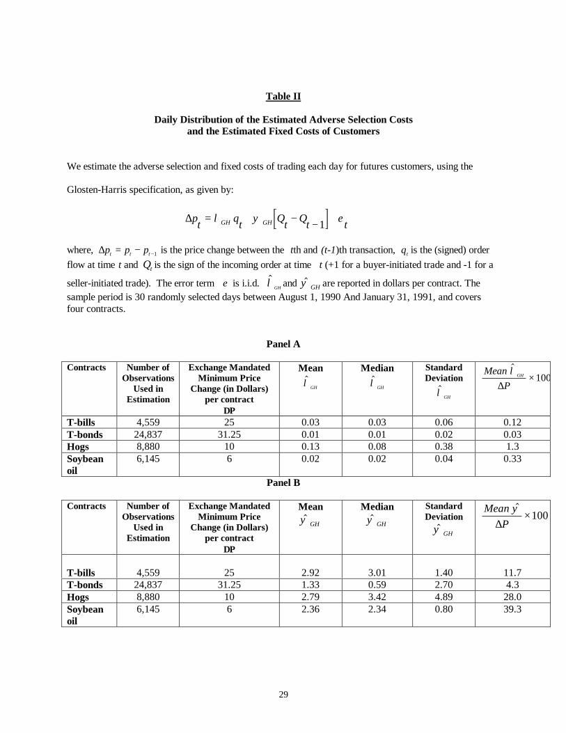
Equation (14) is estimated on a daily basis for each of the four contracts in our sample. 9 Table II

presents the daily distribution of the estimated $λGH and $ψ GH in dollars per contract over the sample

period of thirty days. These estimates are computed over a total of 6,145 observations for the soybeans

futures contract, 8,880 observations for the hog futures, 4,559 observations for the T-bill futures and

24,837 observations for the T-bond futures contract.

The results are broadly consistent with the intuition that the mean adverse selection costs are low

for the Treasury contracts and relatively high for the live hog futures contract. Specifically, the mean

adverse selection cost of trading the T-bill and the T-bond futures is about 3 cents and 1 cent per contract,

respectively. For live hog futures, the mean adverse selection cost is about 13 cents per contract. The

adverse selection cost for soybean oil futures is also low, being about 2 cents per contract.

The fixed costs of trading are higher than the adverse selection costs of trading by several orders

of magnitude. Further, the fixed costs are lower for more active contracts. For the most active contract,

T-Bond futures, the fixed costs are about half that of the other three contracts, all of which are about

equally active. Specifically, the mean fixed costs of trading the T-bill and T-bond futures are given by

$2.92 and $1.33 per contract, respectively. For live hog futures, the mean fixed cost is $2.79 per contract.

For soybean futures, the mean fixed cost is $2.36 per contract.

To provide a sense of the economic magnitude of the adverse selection and fixed costs, we have

expressed the costs as a percentage of the minimum price change or tick size in the contract, as mandated

by the exchange. In liquid futures markets, the minimum tick size is often considered to be a measure of

the average realized bid ask spread of trading the contract. Our results (see Table II) indicate that the

adverse selection cost of trading in the futures contracts studied range from 0.03% to 1.3% of the

9 Some transactions are time-stamped to the same time and have the same price, and for the analysis we treat themas a single transaction, with a price equal to the common price of these transactions and quantity equal to the netquantity. If the time is the same but the prices are different, then we treat these transactions as distinct.

14

minimum tick size. Further, percent adverse selection costs are lowest for the Treasury futures, which is

consistent with intuition. Similarly, the fixed costs of trading range from about 4% to 39% of the

minimum tick size. In comparison, George, Kaul and Nimalendran (1991) report an adverse selection

cost ranging from 8% to 13% of the quoted bid ask spread for small trades on the AMEX/NYSE and

NASDAQ stocks, with the remainder being allocated to fixed costs.

We now turn to our empirical setup.

5. The Number of Informed Traders and Adverse Selection Costs

A. Empirical Set Up

We empirically examine whether the estimated adverse selection cost (the dependent variable) is

correlated with the number of dual traders (the independent variable) in a futures contract. Since the

number of dual traders may itself be determined by the adverse selection cost, the ordinary least squares

(OLS) estimates in regressions where the dependent variable is an estimate of the adverse selection cost

are likely to be biased and inconsistent. To account for the fact that the estimated adverse selection cost

and the number of dual traders in a contract may be determined simultaneously, we adopt a simultaneous

equations (two-stage least squares, or 2SLS) approach.

We include both the daily number of dual traders ( TRADERS) and the daily number of locals

(LOCALS) as endogenous variables in the regression analysis. It is well accepted in the literature that

locals are important suppliers of liquidity in the futures markets. Locals trade frequently during the

trading day by responding to short-run price movements. They hold minimal inventory levels, and trade

in small amounts (see Working (1967), Silber (1984) and Smidt (1985)). Thus, we expect a negative

relationship between $λGH and LOCALS.

Dual traders, when trading for their own accounts, also supply liquidity to the market. However,

to the extent that their trading is based on private information, they increase the adverse selection costs of

15

opposing traders and reduce market liquidity. Therefore, if dual trading is information based, λand

TRADERS may be positively related.

In addition to TRADERS and LOCALS, our endogenous system of variables comprises of the

estimated adverse selection cost, $λGH , and the square of the daily number of dual traders ( TRADERS2).

The term TRADERS2 is included to account for a possible non-monotonic relationship between the

number of dual traders and the adverse selection cost, as predicted by our model.

From an operational standpoint, $λGH is estimated on a daily basis from the Glosten-Harris

regressions, for each contract separately, while the number of dual traders and locals are calculated

according to the procedure described in section 3.

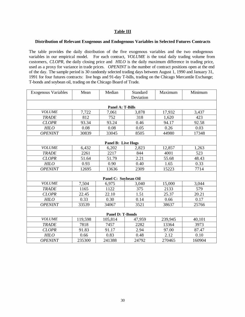
We now turn to identifying the exogenous variables used in the system of equations. For this, we

look for guidance to the extant literature on the determinants of the bid-ask spread ( Benston and

Hagerman (1974), Branch and Freed (1977) and Brennan and Subrahmanyam (1995)). Accordingly, the

five exogenous variables in our system are: (1) VOLUME, the total daily customer trading volume; (2)

TRADE, the daily number of customer trades; (3) C LOPR, the daily closing price; (4) HILO, the daily

maximum difference in trading price, used as a proxy for variance in trade prices; and (5) OPENINT

defined as the daily number of contracts for which delivery is currently obligated, i.e., they are not closed

out. We use OPENINT as a proxy for trading activity and, following Bessembinder and Seguin (1992),

conjecture that the open interest in futures contracts may be correlated with the number of informed

traders. Table III presents some summary statistics on the first five exogenous variables on a contract-by-

contract basis.

Our system of equations is as follows.

$λ εGH a a TRADERS a TRADERS a LOCALS a VOLUME= + + + + +0 1 2 12

3 4 (15)

TRADERS b b b TRADERS b LOCALS b OPENINT b TRADE b HILO b CLOPRGH= + + + + + + + +0 1 2 5 6 7

23 4 2

$λ ε (16)

TRADERS c c c TRADERS c LOCALS c OPENINT c TRADE c HILO c CLOPRGH

2

0 1 2 5 6 73 4 3= + + + + + + + +$λ ε (17)

LOCALS d d d TRADERS d TRADERS d OPENINTGH= + + + + +0 1 22

43 4$λ ε (18)

16

The rank condition provides the necessary and sufficient conditions for identification and

guarantees the estimation of the structural parameters from the reduced form coefficients. Appendix B

provides full details on the rank condition test for model identification. The rank condition indicates that

equations (15) and (18) are identified, while equations (16) and (17) are underidentified. But since our

primary concern is with equation (15), the underidentification of (16) and (17) is not a concern.

We estimate equations (15) and (18) by two-stage least squares (2SLS) for all four futures

contracts. Specifically, 2SLS estimation involves regressing each of the four endogenous variables in our

system on an intercept and the five exogenous variables and computing the predicted values for each

endogenous variable in stage 1. In stage 2, the predicted values of the endogenous variables are used to

estimate the structural equations of the model.

B. The Effect of Dual Trading on Adverse Selection Costs

Table IV reports the 2SLS parameter estimates for the identified equations only (i.e., equations

(15) and (18)) for the four contracts. The estimates are in dollars per contract. The p-value of estimated

parameter significance is reported in parenthesis under each estimate.

Before discussing specific results, we note that the F-statistics for the first stage regression range

from 2.0 to 11.2, and indicate, for all four contracts, a high degree of correlation between the endogenous

variables and the instruments chosen for the empirical analysis.

An increase in the number of dual traders increases the adverse selection costs of trading for

customers in three of the four contracts. In the regression with $λGH as the dependent variable, the

estimated coefficient of TRADERS is positive and statistically significant at the 0.06 level or below in

these contracts. For example, for live hog futures, column (2) of table IV shows that the estimated

coefficient on TRADERS is 0.561 (p-value = 0.063). Similar results hold for soybean oil (column (4)) and

T-Bill futures (Column (6)). For T-bond futures, however, the coefficient of TRADERS in the

$λGH regression is negative (-0.008). We shall have more to say on the T-Bond result later.

17

While $λGH and the number of dual traders are generally positively related, $λGH and the number

of locals are negatively related (statistically significant at the 0.06 level of below) in all four contracts.

For example, for live hog futures, column (2) in table IV shows that the coefficient on LOCALS in the

$λGH regression is -0.204 (p-value = 0.001). Thus, an additional local reduces adverse selection costs by

20 cents per contract in this market. $λGH and LOCALS are negatively related in the soybean oil, T-Bill

and T-Bond contracts as well. 10

The correlation between LOCALS and OPENINT is negative (see columns (3), (5), (7) and (9) of

table IV). For example, column (3) shows that the coefficient on OPENINT in the LOCALS regression

for live hogs, is -0.001 (p-value = 0.057). The results are similar for soybean oil, T-Bills and T-bonds.

Since higher values of OPENINT may indicate increased informed trader activity ( Bessembinder and

Seguin (1991)), this result is consistent with the negative relation between $λGH and LOCALS.

In summary, we show that both the number of dual traders and the number of locals in a c ontract

are significant determinants of the adverse selection cost of trading in a futures contract. However, while

locals appear to supply liquidity to the market, dual traders may reduce liquidity and increase adverse

selection costs – at least for the futures contracts we study.

C. The Non-Monotonicity Result

Recall that proposition 1 implies that we should expect either a single-peaked or a monotonically

decreasing relationship between λand m. In the current section, we investigate the empirical relationship

between λand m. The results are given in table IV.

10 In the regression with LOCALS as the dependent variable, the coefficient of $λGH is negative for three of the four

contracts. For example, in live hog futures (table IV, column (3)), the estimated coefficient for $λGH is –25.811 (p-value = 0.098). The implication is that a $1/contract increase in the adverse selection cost leads to an exit of about26 LOCALS in the live hog futures market. To put these numbers in perspective, notice, from table II, that theaverage adverse selection cost in live hog futures is about $0.13/contract. Thus, from our empirical estimate, a$0.13/contract increase in the adverse selection cost leads to an exit of about 3 LOCALS. For soybean oil and T-Bills, an average increase in adverse selection costs leads to the exit of two to three LOCALS. The coefficient for$λGH is not statistically significant in the T-Bond contract.

18

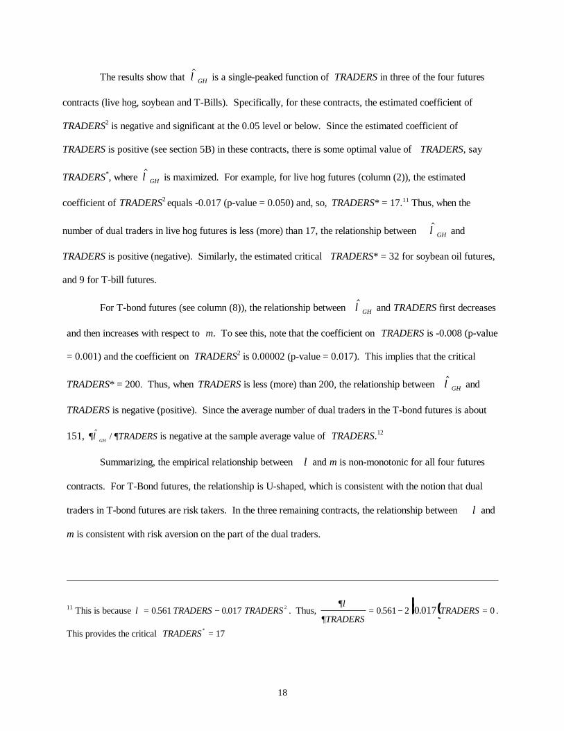
The results show that $λGH is a single-peaked function of TRADERS in three of the four futures

contracts (live hog, soybean and T-Bills). Specifically, for these contracts, the estimated coefficient of

TRADERS2 is negative and significant at the 0.05 level or below. Since the estimated coefficient of

TRADERS is positive (see section 5B) in these contracts, there is some optimal value of TRADERS, say

TRADERS*, where $λGH is maximized. For example, for live hog futures (column (2)), the estimated

coefficient of TRADERS2 equals -0.017 (p-value = 0.050) and, so, TRADERS* = 17.11 Thus, when the

number of dual traders in live hog futures is less (more) than 17, the relationship between $λGH and

TRADERS is positive (negative). Similarly, the estimated critical TRADERS* = 32 for soybean oil futures,

and 9 for T-bill futures.

For T-bond futures (see column (8)), the relationship between $λGH and TRADERS first decreases

and then increases with respect to m. To see this, note that the coefficient on TRADERS is -0.008 (p-value

= 0.001) and the coefficient on TRADERS2 is 0.00002 (p-value = 0.017). This implies that the critical

TRADERS* = 200. Thus, when TRADERS is less (more) than 200, the relationship between $λGH and

TRADERS is negative (positive). Since the average number of dual traders in the T-bond futures is about

151, ∂λ ∂$ /GH TRADERS is negative at the sample average value of TRADERS.12

Summarizing, the empirical relationship between λand m is non-monotonic for all four futures

contracts. For T-Bond futures, the relationship is U-shaped, which is consistent with the notion that dual

traders in T-bond futures are risk takers. In the three remaining contracts, the relationship between λand

m is consistent with risk aversion on the part of the dual traders.

11 This is because λ= −0 561 0 017 2. .TRADERS TRADERS . Thus, ∂λ

∂TRADERSTRADERS= − =0 561 2 00 017. .b g .

This provides the critical TRADERS * = 17

19

6. Dual Trading and Fixed Order Processing Costs

In this section, we examine the relationship between the fixed cost of trading ψ and the number

of dual traders m in a futures contract. Proposition 2 says that we should expect to see either a

monotonically increasing relationship between ψ and m (when the dual traders are risk neutral), or a

U-shaped relationship between ψ and m (when the dual traders are risk averse).

The simultaneous equation system is given by:

$ $λ ψ εGH a a TRADERS a TRADERS a a VOLUMEGH= + + + + +0 1 2 12

3 4 (19)

TRADERS b b b TRADERS b b OPENINT b TRADE b HILO b CLOPRGH GH= + + + + + + + +0 1 2 5 6 7 2

23 4

$ $λ ψ ε (20)

TRADERS c c c TRADERS c c OPENINT c TRADE c HILO c CLOPRGH GH2

0 1 2 5 6 7 33 4= + + + + + + + +$ $λ ψ ε (21)

$ $ψ λ εGH d d d TRADERS d TRADERS d OPENINTGH= + + + + +0 1 22

3 4 4 (22)

where $ψ GH is the estimated fixed cost of trading, obtained from a regression of (14), for the four futures

contracts. The four endogenous variables in the system are: $ψ GH , TRADERS, TRADERS2 and $λGH . The

five exogenous variables are: VOLUME, TRADE, CLOPR, HILO and OPENINT, all defined in section

5A. The difference between the equation system above and the one in (15) - (18) is that we replace

LOCALS with $ψ GH as an endogenous variable. We do this to capture the relationship between $λGH ,

$ψ GH and TRADERS simultaneously, without increasing he number of endogenous variables in the

system.

It is easy to verify that, using the rank condition test of identification in Appendix B, only

equations (19) and (22) are identified. Table V reports the 2SLS parameter estimates (for the identified

equations only) for the four futures contracts. The parameter estimates are denominated in dollars per

contract and the p-values of estimated parameter significance are reported in parenthesis under each

estimate. The first stage regression F-statistics for the contracts range from 2.0 to 13.7, demonstrating

high correlation between the endogenous variables in the system and the chosen instruments.

12 In comparison, ∂λ ∂$ /GH TRADERS for hogs, soybean and T-bills are all positive at their respective sampleaverages.

20

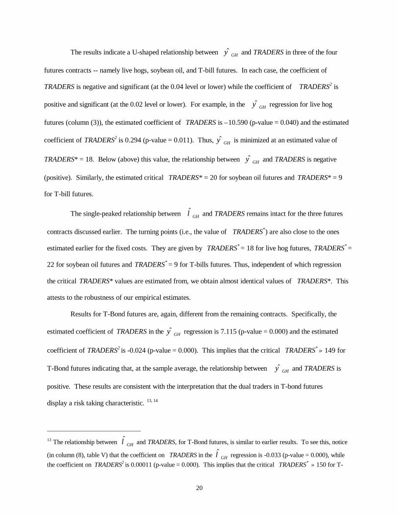
The results indicate a U-shaped relationship between $ψ GH and TRADERS in three of the four

futures contracts -- namely live hogs, soybean oil, and T-bill futures. In each case, the coefficient of

TRADERS is negative and significant (at the 0.04 level or lower) while the coefficient of TRADERS2 is

positive and significant (at the 0.02 level or lower). For example, in the $ψ GH regression for live hog

futures (column (3)), the estimated coefficient of TRADERS is –10.590 (p-value = 0.040) and the estimated

coefficient of TRADERS2 is 0.294 (p-value = 0.011). Thus, $ψ GH is minimized at an estimated value of

TRADERS* = 18. Below (above) this value, the relationship between $ψ GH and TRADERS is negative

(positive). Similarly, the estimated critical TRADERS* = 20 for soybean oil futures and TRADERS* = 9

for T-bill futures.

The single-peaked relationship between $λGH and TRADERS remains intact for the three futures

contracts discussed earlier. The turning points (i.e., the value of TRADERS*) are also close to the ones

estimated earlier for the fixed costs. They are given by TRADERS* = 18 for live hog futures, TRADERS* =

22 for soybean oil futures and TRADERS* = 9 for T-bills futures. Thus, independent of which regression

the critical TRADERS* values are estimated from, we obtain almost identical values of TRADERS*. This

attests to the robustness of our empirical estimates.

Results for T-Bond futures are, again, different from the remaining contracts. Specifically, the

estimated coefficient of TRADERS in the $ψ GH regression is 7.115 (p-value = 0.000) and the estimated

coefficient of TRADERS2 is -0.024 (p-value = 0.000). This implies that the critical TRADERS* ≈ 149 for

T-Bond futures indicating that, at the sample average, the relationship between $ψ GH and TRADERS is

positive. These results are consistent with the interpretation that the dual traders in T-bond futures

display a risk taking characteristic. 13, 14

13 The relationship between $λGH and TRADERS, for T-Bond futures, is similar to earlier results. To see this, notice

(in column (8), table V) that the coefficient on TRADERS in the $λGH regression is -0.033 (p-value = 0.000), whilethe coefficient on TRADERS2 is 0.00011 (p-value = 0.000). This implies that the critical TRADERS* ≈ 150 for T-

21

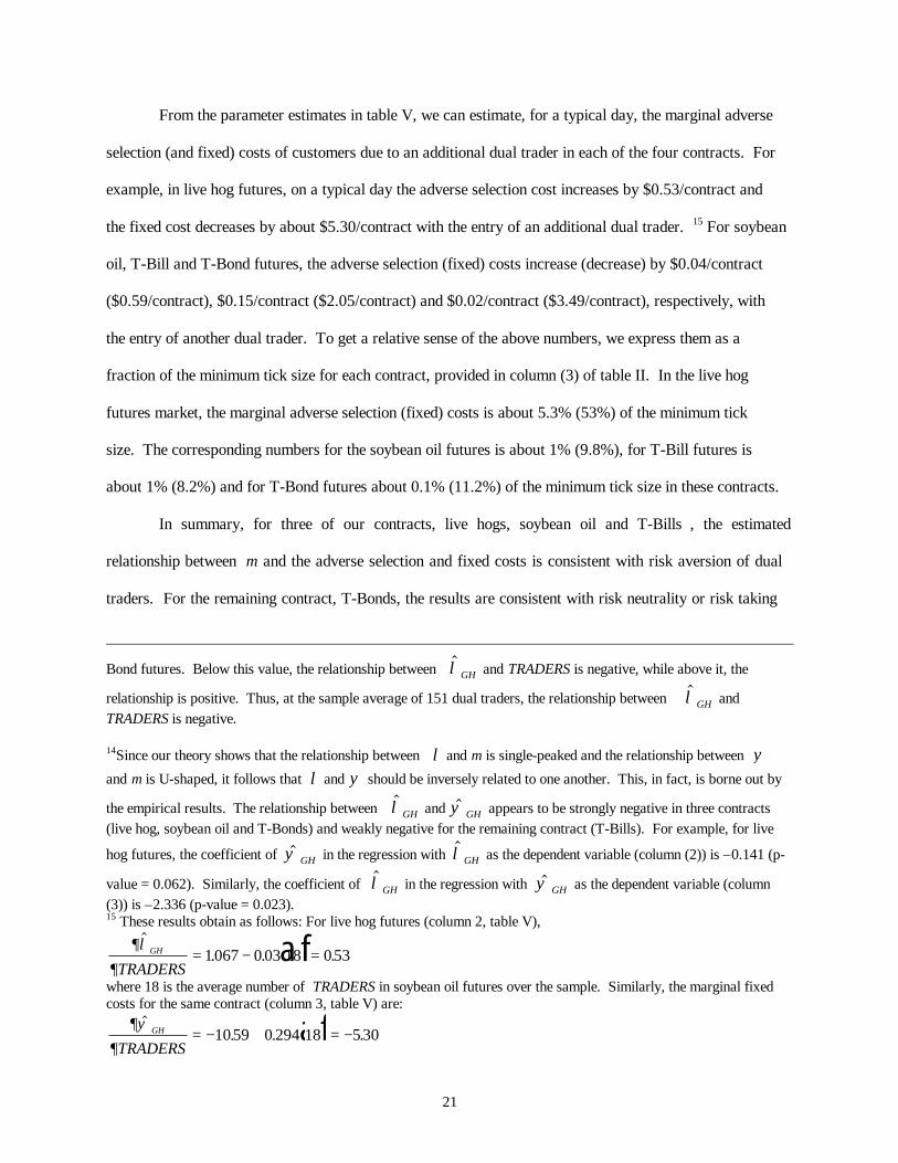
From the parameter estimates in table V, we can estimate, for a typical day, the marginal adverse

selection (and fixed) costs of customers due to an additional dual trader in each of the four contracts. For

example, in live hog futures, on a typical day the adverse selection cost increases by $0.53/contract and

the fixed cost decreases by about $5.30/contract with the entry of an additional dual trader. 15 For soybean

oil, T-Bill and T-Bond futures, the adverse selection (fixed) costs increase (decrease) by $0.04/contract

($0.59/contract), $0.15/contract ($2.05/contract) and $0.02/contract ($3.49/contract), respectively, with

the entry of another dual trader. To get a relative sense of the above numbers, we express them as a

fraction of the minimum tick size for each contract, provided in column (3) of table II. In the live hog

futures market, the marginal adverse selection (fixed) costs is about 5.3% (53%) of the minimum tick

size. The corresponding numbers for the soybean oil futures is about 1% (9.8%), for T-Bill futures is

about 1% (8.2%) and for T-Bond futures about 0.1% (11.2%) of the minimum tick size in these contracts.

In summary, for three of our contracts, live hogs, soybean oil and T-Bills , the estimated

relationship between m and the adverse selection and fixed costs is consistent with risk aversion of dual

traders. For the remaining contract, T-Bonds, the results are consistent with risk neutrality or risk taking

Bond futures. Below this value, the relationship between $λGH and TRADERS is negative, while above it, the

relationship is positive. Thus, at the sample average of 151 dual traders, the relationship between $λGH andTRADERS is negative.

14Since our theory shows that the relationship between λand m is single-peaked and the relationship between ψand m is U-shaped, it follows that λand ψ should be inversely related to one another. This, in fact, is borne out by

the empirical results. The relationship between $λGH and $ψ GH appears to be strongly negative in three contracts(live hog, soybean oil and T-Bonds) and weakly negative for the remaining contract (T-Bills). For example, for live

hog futures, the coefficient of $ψ GH in the regression with $λGH as the dependent variable (column (2)) is –0.141 (p-

value = 0.062). Similarly, the coefficient of $λGH in the regression with $ψ GH as the dependent variable (column(3)) is –2.336 (p-value = 0.023).15 These results obtain as follows: For live hog futures (column 2, table V),

∂λ∂

$. . .GH

TRADERS= − =1067 0 03 18 0 53a f

where 18 is the average number of TRADERS in soybean oil futures over the sample. Similarly, the marginal fixedcosts for the same contract (column 3, table V) are:

∂ψ∂

$. . .GH

TRADERS= − + = −10 59 0 294 18 5 30a f

22

behavior by the dual traders in this contract. This latter result is, perhaps, not surprising since the T-Bond

futures pit is ten times more active than any of the other contracts and it is likely that the active dual

traders in that pit are well capitalized and, consequently, are likely to be either risk neutral or risk takers.

7. A Robustness Check Using an Alternative Measure of Adverse SelectionCost

To ensure that the estimation method does not drive our empirical results, we redo the analysis

using the Madhavan and Smidt (1991) technique to estimate the adverse selection and the fixed cost.

The intuition behind the Madhavan-Smidt (1991) framework is that prices change when new

public information reaches the market as well as in response to trading volume. Thus, a market maker's

posterior expectation of the asset value is a convex combination of the prior mean, which reflects the

public information, and the information contained in the current order flow. The Bayesian weight placed

on the prior mean is a measure of information asymmetry. Formally,

∆Pt Q Q VtQt tt t= − + +−ψπ ψ λ η1 d i (23)

where Qt is defined in section 4, π is the Bayesian weight placed on prior beliefs and Vt is the (unsigned)

order quantity. The error term, ηt , represents unanticipated news events, and, under the assumptions of

the model, follows a MA(1) structure. The moving average structure of the error terms makes the

estimation of (23) a non-linear procedure. The fixed cost (or order processing cost) of transacting an

order of infinitesimal size is given by ψψπ

+FH IK , while the estimated per-contract adverse selection cost

for an order of size Vt is given as λVt . The total cost of trading Vt shares is ψ ψπ

λ+ +FHG

IKJVt .

Note that the Madhavan-Smidt (1991) specification (23) is identical to the Glosten-Harris (1988)

specification (14) only if π = 1 , which implies that the information effect in the current price change

arises only from the current trade.

23

We reestimate the system of equations (19) - (22) using the Madhavan-Smidt procedure and

report results for the two identified equations of the system, equations (19) and (22) only. For brevity, we

report results, in table VI, for only the live hog futures. The results for the other contracts, which are

qualitatively similar, are not reported but available from the authors on request. Specifically, the

relationship between λand m is a single-peaked function for live hogs, soybean oil and T-Bill futures and

U-shaped for T-Bond futures. The relationship between ψ and m is U-shaped for the same three

contracts and single-peaked for the T-Bond futures.

From table VI, the coefficient of TRADERS in the $λMS regression, in column (2), is positive and

significant at the 0.01 level and the coefficient of TRADERS2 is negative and significant at the 0.01 level.

The $ψ MS regression in column (3) indicates that the coefficient of TRADERS is negative and

significant (at the 0.01 level) while the coefficient of TRADERS2 is positive and significant (at the 0.05

level). Thus, the empirical relationship between $λ, $ψ and TRADERS appear to be robust to the method of

estimating the transactions costs.

8. Summary and Conclusions

In this paper we investigate, both theoretically and empirically, the relationship between the

adverse selection and fixed costs of trading and the number of informed traders in a financial asset. We

identify a distinct group of futures floor traders, known as dual traders, as potentially informed traders.

Theoretically, we show that it is optimal for dual traders to derive information from observing their

informed customer's order, and using the information for their own trading. Our empirical examination of

four futures contracts reveals that the number of dual traders on a day is a significant determinant of both

the adverse selection and the fixed costs of trading.

We also examine the relationship between the number of dual traders m and the adverse selection

and fixed costs of trading. Consistent with Subrahmanyam (1991), our model predicts that, if dual traders

24

are risk averse, then the adverse selection costs are a single-peaked function of m. A new prediction of

this paper is that the fixed costs of trading are a U-shaped function of m. For three of the four contracts,

the empirical relationship between m and the adverse selection and fixed costs of trading is as above,

implying that most dual traders in these contracts may be risk averse. For the remaining contract, the T-

Bond futures, the adverse selection (fixed) costs are decreasing (increasing) with m, which is consistent

with dual traders being risk-takers in this contract.

25

References

Admati, A.R., and P. Pfleiderer, A theory of intraday patterns, volume and price variability, Review of

Financial Studies (1988), 1, 3-40.

Bagehot, W., 1971, The only game in town, Financial Analysts Journal, 22, 12-14.

Benston, G., and R. Hagerman, 1974, Determinants of bid-ask spreads in the over-the-counter market,

Journal of Financial Economics, 1, 353-364.

Bessembinder, H., and P. Seguin, 1992, Futures-Trading Activity and Stock Price Volatility, Journal of

Finance, 47, 2015-2034.

Branch, B., and W. Freed, 1977, Bid-asked spreads on the AMEX and the big board, Journal of Finance,

32, 159-163.

Brennan, M.J., N. Jegadeesh, and B. Swaminathan, 1993, Investment analysis and the adjustment of stock

prices to common information , Review of Financial Studies, 6, 799-824.

Brennan, M.J. and A. Subrahmanyam, 1995, Investment analysis and price formation in securities

markets, Journal of Financial Economics, 38, 361-381.

Brennan, M.J. and A. Subrahmanyam, 1998, The determinants of average trade size , Journal of Business,

71, 1-25.

Chakravarty, S., 1994, Should actively traded futures contracts come under the dual trading ban ?, The

Journal of Futures Markets, 14, 661-684.

Chang, E., P. R. Locke, and S.C. Mann, 1994, The effect of CME Rule 552 on dual traders, Journal of

Futures Markets, 14, 493-510.

Copeland, T., and D. Galai, 1983, Information effects and the bid-ask spread, Journal of Finance, 38,

1457-1469.

Fishman, M.J., and F. A. Longstaff, 1992, Dual trading in futures markets, Journal of Finance, 47, 643-

671.

Glosten, L.R., and L. Harris, 1988, Estimating the components of the bid-ask spread, Journal of Financial

Economics, 21, 123-142.

26

George, T.J., G. Kaul and M. Nimalendran, 1991, Estimation of the bid ask spread and its components ; A

new approach, Review of Financial Studies, 4, 623-656.

Glosten, L.R., and P.R. Milgrom, 1985, Bid, ask and transaction prices in a specialist market with

heterogeneously informed traders , Journal of Financial Economics, 14, 71-100.

Greene, W.H., 1997, Econometric Analysis, third edition, Prentice Hall. New Jersey.

Grossman, S.J., 1989, An economic analysis of dual trading, working paper, University of Pennsylvania.

Hasbrouck, J., 1991, Measuring the information content of stock trades, Journal of Finance, 46, 179-207.

Kyle, A.S.,1985, Continuous auctions and insider trading, Econometrica, 53, 1315-1335.

Locke, P., A. Sarkar, and L. Wu, 1998, Market liquidity and trader welfare in multiple dealer markets,

working paper, the Federal Reserve Bank of New York.

Madhavan, A., and S. Smidt, 1991, A Bayesian model of intraday specialist pricing, Journal of Financial

Economics, 30, 99-134.

Manaster, S., and S.C. Mann, 1996, Life in the pits: Competitive market making and inventory control,

Review of Financial Studies, 9, 953-975.

Roell, A., 1990, Dual capacity trading and the quality of the market, Journal of Financial Intermediation,

1, 105-124.

Sarkar, A., 1995, Dual trading: winners, losers and market impact, Journal of Financial Intermediation,

4, 77-93.

Silber, W.L., 1984, Market maker behavior in an auction market: An analysis of scalpers in futures

markets, Journal of Finance, 39, 937-953.

Smidt, S., 1985, Trading floor practices on futures and securities exchanges: economics, regulation and

policy issues, Futures Markets: Regulatory Issues, American Institute for Public Policy Research,

Washington, D.C.

Subrahmanyam, A., 1991, Risk aversion, market liquidity and price efficiency, Review of Financial

Studies, 4, 417-441.

27

Working, H., 1967, Tests of a theory concerning floor-trading on Commodity Exchanges, Food Research

Institute Studies: Supplement.

28

Table I

Daily Number of Dual Traders and Locals in Selected Futures Pits

The table gives the distribution of the daily number of dual traders ( TRADERS) and the daily number oflocals (LOCALS) for each of the four futures contracts. A dual trader is defined as a floor trader who tradesboth for her own account and for her customers during a trading day. A local is a floor broker who tradesexclusively for her own account during a trading day. The sample period is 30 randomly selected tradingdays between August 1, 1990 and January 31, 1991 for four futures contracts : live hogs and 91 day T-bills,trading on the Chicago Mercantile Exchange; T-bonds and soybean oil, trading on the Chicago Board ofTrade.

Live hogs Soybean oil T-bills T-bonds

Average dailycustomer tradingvolume(CUSTOMERVOLUME)

6,432 7,504 7,722 119,598

Number of dual traders (TRADERS)

Mean 17.5 18.93 8.54 151.1

Standard deviation 3.14 3.21 1.93 12.31

Minimum 9 14 5 117

1st Quartile 16 16 7 143

Median 18 18 9 153

3rd Quartile 19 21 10 161

Maximum 23 27 13 168

Panel B: Number of Locals (NOLOC)

Mean 15.87 10.80 23.47 202.1

Standard deviation 2.15 3.45 4.35 25.22

Minimum 11 4 14 114

1st Quartile 14 8 21 195

Median 16 11 24 207

3rd Quartile 17 12 26 215

Maximum 21 20 36 243

29

Table II

Daily Distribution of the Estimated Adverse Selection Costsand the Estimated Fixed Costs of Customers

We estimate the adverse selection and fixed costs of trading each day for futures customers, using the

Glosten-Harris specification, as given by:

∆pt qt Qt Qt tGH GH= + − − +λ ψ ε1

where, ∆p p pt t t= − − 1 is the price change between the tth and (t-1)th transaction, qt is the (signed) orderflow at time t and Qt is the sign of the incoming order at time t (+1 for a buyer-initiated trade and -1 for a

seller-initiated trade). The error term ε is i.i.d. $λGH and $ψ GH are reported in dollars per contract. Thesample period is 30 randomly selected days between August 1, 1990 And January 31, 1991, and coversfour contracts.

Panel A

Contracts Number ofObservations

Used inEstimation

Exchange MandatedMinimum Price

Change (in Dollars)per contract

∆P

Mean$λGH

Median$λGH

StandardDeviation

$λGH

MeanP

GH $λ∆

×100

T-bills 4,559 25 0.03 0.03 0.06 0.12T-bonds 24,837 31.25 0.01 0.01 0.02 0.03Hogs 8,880 10 0.13 0.08 0.38 1.3Soybeanoil

6,145 6 0.02 0.02 0.04 0.33

Panel B

Contracts Number ofObservations

Used inEstimation

Exchange MandatedMinimum Price

Change (in Dollars)per contract

∆P

Mean$ψ GH

Median$ψ GH

StandardDeviation

$ψ GH

MeanP

$ψ∆

×100

T-bills 4,559 25 2.92 3.01 1.40 11.7T-bonds 24,837 31.25 1.33 0.59 2.70 4.3Hogs 8,880 10 2.79 3.42 4.89 28.0Soybeanoil

6,145 6 2.36 2.34 0.80 39.3

30

Table III

Distribution of Relevant Exogenous and Endogenous Variables in Selected Futures Contracts

The table provides the daily distribution of the five exogenous variables and the two endogenousvariables in our empirical model. For each contract, VOLUME is the total daily trading volume fromcustomers, CLOPR, the daily closing price and HILO is the daily maximum difference in trading price,used as a proxy for variance in trade prices. OPENINT is the number of contract positions open at the endof the day. The sample period is 30 randomly selected trading days between August 1, 1990 and January 31,1991 for four futures contracts: live hogs and 91-day T-bills, trading on the Chicago Mercantile Exchange;T-bonds and soybean oil, trading on the Chicago Board of Trade.

Exogenous Variables Mean Median StandardDeviation

Maximum Minimum

Panel A: T-BillsVOLUME 7,722 7,061 3,878 17,932 3,437TRADE 812 752 318 1,620 423CLOPR 93.34 93.24 0.46 94.17 92.58HILO 0.08 0.08 0.05 0.26 0.03

OPENINT 30839 33045 8505 44980 17348

Panel B: Live HogsVOLUME 6,432 6,202 2,823 12,857 1,263TRADE 2261 2217 844 4001 523CLOPR 51.64 51.79 2.21 55.68 48.43HILO 0.93 0.90 0.40 1.65 0.33

OPENINT 12695 13636 2309 15223 7714

Panel C: Soybean OilVOLUME 7,504 6,975 3,040 15,000 3,044TRADE 1165 1122 375 2133 579CLOPR 22.45 22.10 1.51 25.37 20.21HILO 0.33 0.30 0.14 0.66 0.17

OPENINT 33539 34067 3521 38637 25766

Panel D: T-BondsVOLUME 119,598 105,814 47,959 239,945 40,101TRADE 7818 7457 2282 13364 3973CLOPR 91.83 91.17 2.94 97.00 87.47HILO 0.66 0.83 0.48 2.12 0.10

OPENINT 235300 241388 24792 270465 160904

31

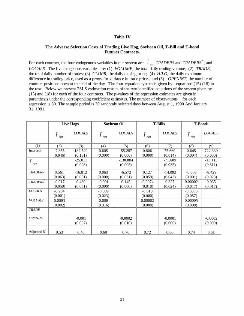
Table IV

The Adverse Selection Costs of Trading Live Hog, Soybean Oil, T-Bill and T-bondFutures Contracts.

For each contract, the four endogenous variables in our system are $λGH

, TRADERS and TRADERS2 , andLOCALS. The five exogenous variables are: (1) VOLUME, the total daily trading volume; (2) TRADE,the total daily number of trades; (3) CLOPR, the daily closing price; (4) HILO, the daily maximumdifference in trading price, used as a proxy for variance in trade prices; and (5) OPENINT, the number ofcontract positions open at the end of the day. The four-equation system is given by equations (15)-(18) inthe text. Below we present 2SLS estimation results of the two identified equations of the system given by(15) and (18) for each of the four contracts. The p-values of the regression estimates are given inparenthesis under the corresponding coefficient estimates. The number of observations for eachregression is 30. The sample period is 30 randomly selected days between August 1, 1990 And January31, 1991.

Live Hogs Soybean Oil T-Bills T-Bonds

$λGHLOCALS $λGH

LOCALS $λGHLOCALS $λGH

LOCALS

(1) (2) (3) (4) (5) (6) (7) (8) (9)Intercept -7.355

(0.046)182.529(0.131)

0.605(0.000)

-55.287(0.000)

0.806(0.000)

75.669(0.014)

0.645(0.004)

722.330(0.000)

$λGH-25.811(0.098)

-130.884(0.005)

-71.609(0.035)

-13.113(0.811)

TRADERS 0.561(0.063)

-16.812(0.051)

0.063(0.000)

-6.572(0.031)

0.127(0.059)

-14.092(0.043)

-0.008(0.001)

-8.429(0.023)

TRADERS2 -0.017(0.050)

0.480(0.031)

-0.001(0.000)

0.145(0.000)

-0.0074(0.010)

0.827(0.024)

0.00002(0.017)

0.035(0.017)

LOCALS -0.204(0.001)

-0.009(0.023)

-0.018(0.000)

-0.0006(0.057)

VOLUME 0.0003(0.002)

0.000(0.316)

0.00002(0.000)

0.00005(0.000)

TRADE

OPENINT -0.001(0.057)

-0.0002(0.010)

-0.0001(0.000)

-0.0002(0.000)

Adjusted R2 0.53 0.40 0.68 0.70 0.72 0.66 0.74 0.61

32

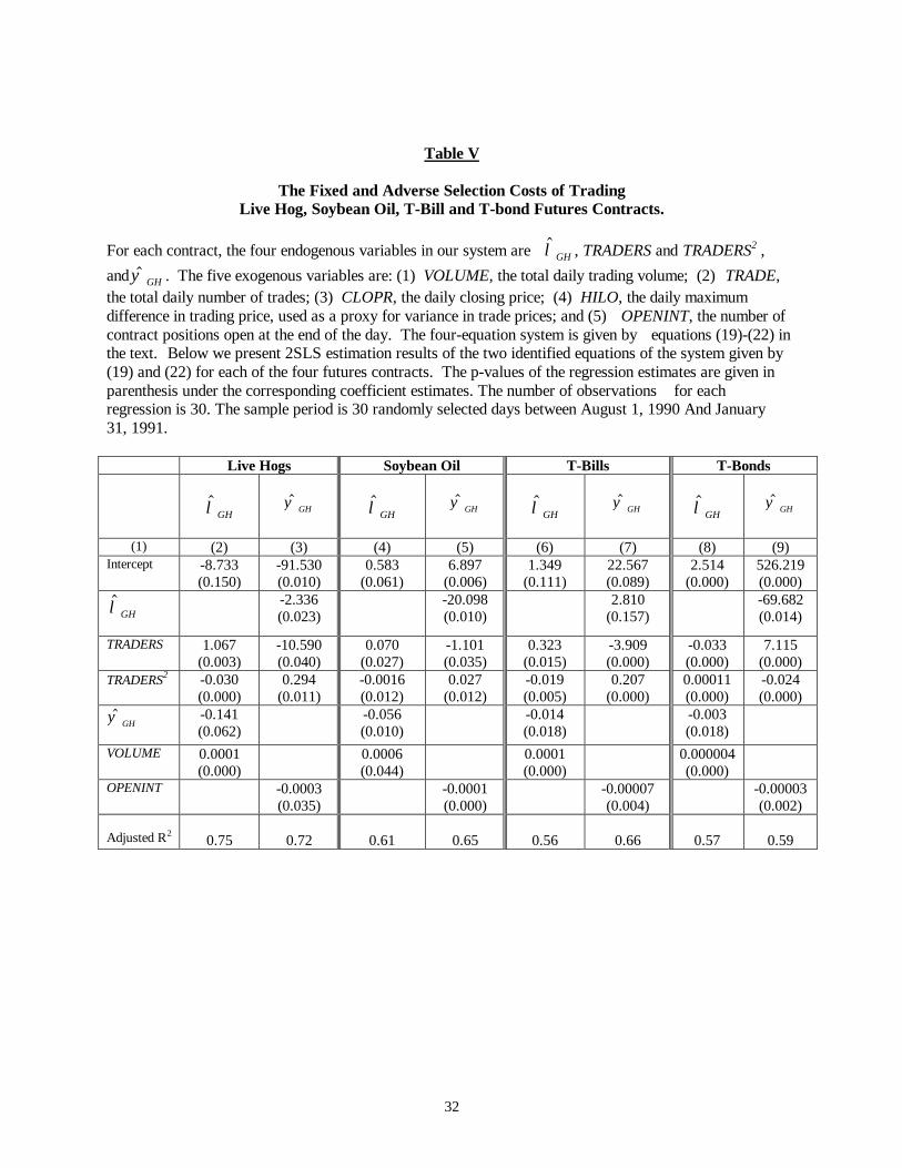
Table V

The Fixed and Adverse Selection Costs of TradingLive Hog, Soybean Oil, T-Bill and T-bond Futures Contracts.

For each contract, the four endogenous variables in our system are $λGH , TRADERS and TRADERS2 ,and $ψ GH . The five exogenous variables are: (1) VOLUME, the total daily trading volume; (2) TRADE,the total daily number of trades; (3) CLOPR, the daily closing price; (4) HILO, the daily maximumdifference in trading price, used as a proxy for variance in trade prices; and (5) OPENINT, the number ofcontract positions open at the end of the day. The four-equation system is given by equations (19)-(22) inthe text. Below we present 2SLS estimation results of the two identified equations of the system given by(19) and (22) for each of the four futures contracts. The p-values of the regression estimates are given inparenthesis under the corresponding coefficient estimates. The number of observations for eachregression is 30. The sample period is 30 randomly selected days between August 1, 1990 And January31, 1991.

Live Hogs Soybean Oil T-Bills T-Bonds

$λGH$ψ GH $λGH

$ψ GH $λGH$ψ GH $λGH

$ψ GH

(1) (2) (3) (4) (5) (6) (7) (8) (9)Intercept -8.733

(0.150)-91.530(0.010)

0.583(0.061)

6.897(0.006)

1.349(0.111)

22.567(0.089)

2.514(0.000)

526.219(0.000)

$λGH-2.336(0.023)

-20.098(0.010)

2.810(0.157)

-69.682(0.014)

TRADERS 1.067(0.003)

-10.590(0.040)

0.070(0.027)

-1.101(0.035)

0.323(0.015)

-3.909(0.000)

-0.033(0.000)

7.115(0.000)

TRADERS2 -0.030(0.000)

0.294(0.011)

-0.0016(0.012)

0.027(0.012)

-0.019(0.005)

0.207(0.000)

0.00011(0.000)

-0.024(0.000)

$ψ GH-0.141(0.062)

-0.056(0.010)

-0.014(0.018)

-0.003(0.018)

VOLUME 0.0001(0.000)

0.0006(0.044)

0.0001(0.000)

0.000004(0.000)

OPENINT -0.0003(0.035)

-0.0001(0.000)

-0.00007(0.004)

-0.00003(0.002)

Adjusted R2 0.75 0.72 0.61 0.65 0.56 0.66 0.57 0.59

33

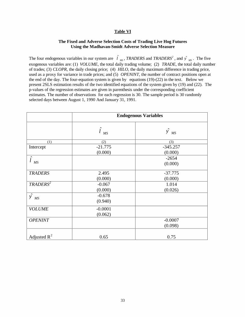
Table VI

The Fixed and Adverse Selection Costs of Trading Live Hog FuturesUsing the Madhavan-Smidt Adverse Selection Measure

The four endogenous variables in our system are $λMS , TRADERS and TRADERS2 , and $ψ MS . The fiveexogenous variables are: (1) VOLUME, the total daily trading volume; (2) TRADE, the total daily numberof trades; (3) CLOPR, the daily closing price; (4) HILO, the daily maximum difference in trading price,used as a proxy for variance in trade prices; and (5) OPENINT, the number of contract positions open atthe end of the day. The four-equation system is given by equations (19)-(22) in the text. Below wepresent 2SLS estimation results of the two identified equations of the system given by (19) and (22). Thep-values of the regression estimates are given in parenthesis under the corresponding coefficientestimates. The number of observations for each regression is 30. The sample period is 30 randomlyselected days between August 1, 1990 And January 31, 1991.

Endogenous Variables

$λMS$ψ MS

(1) (2) (3)Intercept -21.775

(0.000)-345.257(0.000)

$λMS-2654

(0.000)

TRADERS 2.495(0.000)

-37.775(0.000)

TRADERS2 -0.067(0.000)

1.014(0.026)

$ψ MS-0.678(0.940)

VOLUME -0.0001(0.062)

OPENINT -0.0007(0.098)

Adjusted R2 0.65 0.75

34

Figure 1

Note: (1) corresponds to R=2; Σ u =1; Σ v =1. (2) corresponds to R=2; Σ u =5; Σ v =6.

(3) corresponds to R=2; Σ u =5; Σ v =2

Lambda_2 Versus m

0.15

0.2

0.25

0.3

0.35

0.4

1 2 3 4 5 6 7 8 9 10

m

Lambda_2 (1)Lambda_2 (2)Lambda_2 (3)

35

Appendix A

Proof of Lemma 1:

We know from equation (3) in the text that broker j's profits are given by:

Π j j j j j jz v z z u z p z= − + + −−λ2 2 1d i (A.1)

Further, each risk averse broker maximizes an objective function given by

E x pR

Var x pj jΠ Π, ,1 12d i d i−

Now,

E x p z E v x z z z p zj j j j jjΠ , 1 2

2

2 1e j e j e j= − − −−λ λand,

Var x p E u zj j∏ = −, 1 2 2

2e j λ (A.2)

= λ22 2b g d iz j uΣ

The jth broker's objective function can now be formally expressed as:Maxz z x z z z p z

Rz

jj j j j j j u2

21 2

2

2 1 22 2λ λ λ λ− − − −−d i b g d i Σ (A.3)

From the first order condition, we have

z m Rj u2 12 2 22λ λ λ+ − +b g b g Σ = 2 1 1 1 1 1λ λx p x u− = −b g (A.4)

or, zx u

m Rj

u

= −+ +λ

λ λ1 1 1

2 221

b gb g b g Σ

(A.5)

(QED)Proof of Lemma 2:

We start from the fact that

y mz um x u

Duj2 2

1 1 12= + = − +λ b g

(A.6)

where D = λ λ2 21+ +m R ub g Σ

Given that λ22

2

= Cov v yVar y

,b gb g ,

36

λ

λλ

λλ

2

1

12

12

12

2

4

=⋅

+FHG

IKJ+

LNM

OQP

D2

mD

m

v

vu u

Σ

Σ Σ Σ

or, λλ2 2 2

12 2

24 4

=+ +

mDm m D

v

v u u

ΣΣ Σ Σ

or, λ λ2 2 2 2 122

414

=+ +

=LNM

OQP

mDm m D

v

v v u

v

u

ΣΣ Σ Σ

ΣΣ

Q

or, λ2 2 2 12=

+≡mD

m Df Dv

v u

ΣΣ Σ b g (A.7)

Note that when R = 0, (A.7) reduces to (8) in the text. This proves part (1) of Lemma 2.

When R > 0, (A.7) is the same as (9) in the text.(QED)

Proof of Lemma 3:

Denote z B x B pj = +1 2 1 . From the first order condition given by (A.4),

BD

BD1

12

2 1= = −λ and

Note from above that B B1 1 22= − λ . So, if we know B2, we also know B1. To establish theexistence of a unique λ2 > 0, we follow the method of proof indicated in proposition 1 ofSubrahmanyam (1991). We have:

BD m R u

22 2

2

1 11

= − = −+ +λ λb g b g Σ

or, λ λ22

2 2 2 1 1 0b g b gRB B mu + + + = Σ (A.8)

Clearly, λ2 must satisfy both (A.8) and (A.7). (A.8) has only one positive real root (for a givenB2), given by:

f Dm

Rm RD

RD

Bu

u

u2 2

2

2

12

1 42

1b g b g b g≡ = − + ++ +

= −LNM

OQPλ

ΣΣ

Σ Q (A.9)

37

Thus, λ2 and D are determined by the point where f D1b g and f D2b g intersect in λ2 − D space.In what follows, we assume that (A.7) and (A.8) hold.

Lemma A1: fdfdD

d fdD2

22

220 0 0 0b g= , , . > <

Proof of lemma A1: follows directly from definition of f D2b g in (A.9).(QED)

Lemma A2: f1 0 0b g= and, further, f D1b g is unimodal, reaching a maximum at

D m v

u

* = ΣΣ2

Proof of lemma A2:

f1 0 0b g= from definition. To show unimodality, we show that d f D

dD

21

2

b g < 0 at all

points where df D

dD1 0b g= .

df DdD

mm D

m DD

mv

v u

v u

v

u

12 2

2 2 22

22

20

2b g= ⋅ −

+= =Σ Σ Σ

Σ ΣΣΣ

at or at D m v

u

= ΣΣ2

. (A.10)

d f DdD

D m

m Dmu v

v u

v

21

2

2

2 2 4

8

2

b gc h= −

+⋅Σ Σ

Σ ΣΣ (A.11)

= − 8

4

3 2

4 2 2

D m

mu v

v

Σ ΣΣ

at D

m v

u

22

2= Σ

Σ

= − ⋅12 5 2

Dm

u

v

ΣΣ

< 0(A.12)

From lemma A1 and lemma A2, either f D1b g and f D2b g never intersect, or theyintersect only once.

(QED)

38

Lemma A3: f D f D1 2b g b g and have a unique intersection.

Proof of lemma A3:

f D f D1 2b g b g and intersect if:

dfdD

dfdD

1 20 0b g b g > (A.13)

dfdD m

D1 0 10b g = at = , from (A.10)

df DdD

m RD u

2

21 4

b gb g

= 1

+ 12+ Σ

= at 1

10

+=

mD

(QED)

Hence, df dD df dD1 20 0b g b g/ /> and there exists a unique real root λ2 . This proves lemma 3.(QED)

Proof of Proposition 1:

We will show:ddm

ddm

22

220 0

λ λ < at =

Consider (A.7) again:

λλ λ

2

+ +

=+m m R

m Dv u

v u

Σ ΣΣ Σ

2 22 2

12

b gm r

or 1 = 2

m m Rm Dv

v u

Σ ΣΣ Σ1

22 2

2

+ ++

b gm rλ(A.14)

Let y = 2 22D m m Ru v v uΣ Σ Σ Σ − − λ (A.15)

where (A.15) follows from writing (A.14) in implicit form.

∴ ddm

y my

λλ

2

2

= − ∂ ∂∂ ∂

//

39

Now, ∂∂

∂∂

yD

DR mu u vλ λ2 2

4 = - Σ Σ Σ

= Σ Σu vDD

R m42

∂∂

−LNM

OQPλ

= + - Σ Σ Σu u vDD

R R m42λ

FHG

IKJ

LNM

OQP

> 0.

The last inequality follows because from (A.14), we have:

2 2

2 2

D mR m R mv

uv vλ λ

= + > Σ

ΣΣ Σ

Since∂∂

∂ ∂y ddmλλ

2

2 > 0, = 0 if y / m = 0 .

To show that λ2 is unimodal with respect to m, we will showddm

dd

2

2

λ λ < 0 when

m = 0, or equivalently,2 when ∂ ∂y m/ = 0.

ddm

ddm

y m

yym

22

22

λλ

= at = 0.− ∂ ∂

∂ ∂∂∂

/

/

b g(A.16)

So, ∂ λ∂

22

2md

dmy m < 0 if < 0.− ∂ ∂/b g

∂∂

∂∂

⋅ − − ∂∂

−ym

DDm

Rmm

Rv u v u v = 4 uΣ Σ Σ Σ Σ Σλ λ22

ddm

ym

Dd

dmDm

Dm

Dm

R md

dmu u u v m

2− ∂∂

= − ⋅∂∂

− ⋅∂∂

+ ⋅∂∂

FH IK FH IK FHG

IKJ FH IK4 4Σ Σ Σ Σ∂

∂λ

, atddmλ2 0 =

= − − +FHG

IKJ−

LNM

OQP4 42

22

22

2

λ λλb g Σ Σ Σ Σu u u m v

ddm

DD

R R (A.17)

From (A.16) and (A.17)

40

ddm

yD

DR Rmu u v

22

22 2

4λ

∂λ λ∂ + +F

HGIKJ−

LNM

OQP

RS|T|UV|W|

Σ Σ Σ = − 4 22λb g Σu

As shown earlier, 2 2

2 2

DR m vλ ∂λ

> and, further, y

> 0.Σ ∂ Hence, ddm

22

2

λ < 0.

(QED)

Proof of Proposition 2:

Let E z fe jdenote the expected trading volume per broker, which is proportional to the standard

deviation of z f . From (12) in the text

E zD

hfr

r re j= F

HGIKJ−

LNM

OQP

2σ ψσ

ψσ

(A.18)

(A.18) is derived in Brennan and Subrahmanyam (1998). h rψ σ/b gis the hazard function

defined by

h xx

x( ) =

−φb g

b g1 Φ

where φ xb gis the standard normal density function and Φ xb gis the standard normal distribution.

From (A.18),

dE z

dm DH D D

ddm D

Hddm

f rm

e j= − +F

HGIKJ+2 2

22

2

σ λ ψλ ψ (A.19)

where, H hr r

= FHG

IKJ−ψ

σψσ

, DDmm = ∂

∂, D

Dλ

∂∂λ2

2

= and HH

ψ∂∂ψ

= .

Assumption: dE z

dmfe j

= 0

41

The above assumption implies that the brokerage industry is in long-term competitive

equilibrium. The entry of an additional broker has no effect on any broker's expected trading

volume.

Given our assumption, (A.19) implies:

ddm

DH D D d

dmH

rmψ

σ λλ

ψ=

+FHG IKJ2

2

(A.20)

From the proof of proposition 2 in Brennan and Subrahmanyam (1998), H > 0 and

H hr

ψψσ

= FHG

IKJ− <' 1 0

Now suppose R = 0. Then,

D Dddm m

mm

m

m

mv

u

+ = − ++

LNM

OQP

< ≥

λλ

2

2 2

21

1

0 2

ΣΣ c h

for .

Hence, when R = 0, ddmψ

> 0 for m ≥ 2. This proves part 1 of proposition 2.

Now suppose R > 0. Then for small m, ddmλ2 0> , and

D Dddm

mddmm + = + + >λ

λ λ λ2

22

22 1 0b g (A.21)

Hence, from (A.20), ddmψ < 0 for small m.

For large m, ddmλ2 0< and, from (A.21), D D

ddmm + <λλ

2

2 0 is likely since the negative term is

proportional to m and, hence, likely to dominate.

Hence, from (A.20), ddmψ > 0 is positive for large m.

(QED)

42

Appendix B

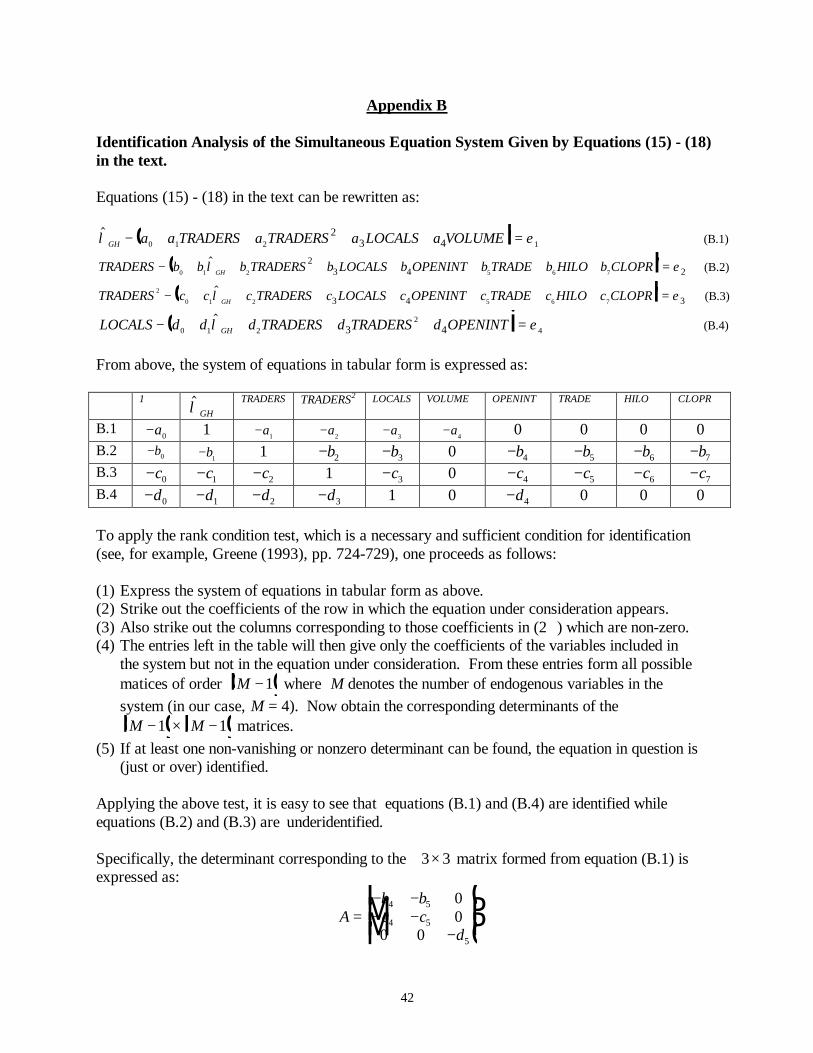
Identification Analysis of the Simultaneous Equation System Given by Equations (15) - (18)in the text.

Equations (15) - (18) in the text can be rewritten as:

$λ εGH a a TRADERS a TRADERS a LOCALS a VOLUME− + + + + =0 1 2 12

3 4c h (B.1)

TRADERS b b b TRADERS b LOCALS b OPENINT b TRADE b HILO b CLOPRGH− + + + + + + + =0 1 2 5 6 7

23 4 2

$λ εc h (B.2)

TRADERS c c c TRADERS c LOCALS c OPENINT c TRADE c HILO c CLOPRGH

2

0 1 2 5 6 73 4 3− + + + + + + + =$λ εc h (B.3)

LOCALS d d d TRADERS d TRADERS d OPENINTGH− + + + + =0 1 22

43 4$λ εd i (B.4)

From above, the system of equations in tabular form is expressed as:

1 $λGHTRADERS TRADERS2 LOCALS VOLUME OPENINT TRADE HILO CLOPR

B.1 − a0 1 − a1 − a2 − a3 − a4 0 0 0 0B.2 − b0 − b1 1 − b2 − b3 0 − b4 − b5 − b6 − b7

B.3 − c0 − c1 − c2 1 − c3 0 − c4 − c5 − c6 − c7

B.4 − d0 − d1 − d2 − d3 1 0 − d4 0 0 0

To apply the rank condition test, which is a necessary and sufficient condition for identification(see, for example, Greene (1993), pp. 724-729), one proceeds as follows:

(1) Express the system of equations in tabular form as above.(2) Strike out the coefficients of the row in which the equation under consideration appears.(3) Also strike out the columns corresponding to those coefficients in (2 ) which are non-zero.(4) The entries left in the table will then give only the coefficients of the variables included in

the system but not in the equation under consideration. From these entries form all possiblematices of order M − 1b g where M denotes the number of endogenous variables in thesystem (in our case, M = 4). Now obtain the corresponding determinants of the

M M− × −1 1b g b g matrices.(5) If at least one non-vanishing or nonzero determinant can be found, the equation in question is

(just or over) identified.

Applying the above test, it is easy to see that equations (B.1) and (B.4) are identified whileequations (B.2) and (B.3) are underidentified.

Specifically, the determinant corresponding to the 3 3× matrix formed from equation (B.1) isexpressed as:

Ab bc c

d=

− −− −

−

LNMM

OQPP

4 5

4 5

5

00

0 0

43

with the corresponding determinant given by:

det A b c d b c db g b g b g= − − − − ≠4 5 5 5 4 50 0 0

The above implies that equation (B.1) is identified. The remaining equations follow similarly.