estimating roadside encroachment rates with the combined ... · encroachment rates for rural...
TRANSCRIPT
ESTIMATING ROADSIDE ENCROACHMENT RATES WITH THE COMBINED STRENGTHS OF ACCIDENT-
AND ENCROACHMENT-BASED APPROACHES
FINAL REPORT
Publication No. FHWA-RD-01-124
Shaw-Pin Miaou, Ph.D. Safety and Structural Systems Division
Texas Transportation Institute Texas A&M University System
College Station, Texas 77843-3135 (979) 862-8753

FOREWORD
This report assesses the consistency of estimating vehicle roadside encroachment rates usingaccident-based prediction models. The research used two data sets developed from FHWA'sHighway Safety Information System. These data are more recent than those reported in theprevious assessments. By synthesizing the models developed from this and previous studies, aroadside encroachment rate estimation model was recommended. The model allows theencroachment rates to be estimated by average annual daily traffic volume, lane width,horizontal curvature, and vertical grade for rural two- lane undivided roads.
Michael F. TrentacosteDirector, Office of Safety Research & Development
NOTICE
This document is disseminated under the sponsorship of the Department of Transportation in theinterest of information exchange. The United States Government assumes no liability for itscontents or use thereof. This report does not constitute a standard, specification, or regulation.The United States Government does not endorse products or manufacturers. Trade andmanufacturers’ names appear in this report only because they are considered essential to theobject of the document.

Technical Report Documentation Page 1. Report No. FHWA-RD-01-124
2. Government Accession No. 3. Recipient's Catalog No.
5. Report Date September 2001
4. Title and Subtitle ESTIMATING ROADSIDE ENCROACHMENT RATES WITH THE COMBINED STRENGTHS OF ACCIDENT- AND ENCROACHMENT-BASED APPROACHES
6. Performing Organization Code
7. Author(s) S.P. Miaou
8. Performing Organization Report No.
10. Work Unit No. (TRAIS)
9. Performing Organization Name and Address Oak Ridge National Laboratory Attn: Pat Hu P.O. Box 2008 Bldg. 3156, MS-6073 Oak Ridge, TN 37831
11. Contract or Grant No. DTFH61-94-Y-00107
13. Type of Report and Period Covered Final Report February 28, 1998 – September 21, 2001
12. Sponsoring Agency Name and Address Federal Highway Administration Turner-Fairbanks Highway Research Center 6300 Georgetown Pike McLean, VA 22101-2296 14. Sponsoring Agency Code
15. Supplementary Notes Contracting Officer’s Technical Representative (COTR’s): Joe Bared 16. Abstract In two recent studies by Miaou, he proposed a method to estimate vehicle roadside encroachment rates using accident-based models. He further illustrated the use of such method to estimate roadside encroachment rates for rural two- lane undivided roads using data from the Seven States Cross-Section Data Base of Federal Highway Administration [FHWA]. The results of his study indicated that the proposed method could be a viable approach to estimating roadside encroachment rates without actually collecting the encroachment data in the field, which can be expensive and technically difficult. This study tested the consistency of Miaou’s approach using two data sets from FHWA’s Highway Safety Information System (HSIS). In addition, by synthesizing the models developed from this and previous studies, a roadside encroachment rate estimation model was recommended. The model allows the rates to be estimated by average annual daily traffic volume, lane width, horizontal curvature, and vertical grade for rural two- lane undivided roads. 17. Key Word Roadside Encroachment, Roadway Geometric, Accident Prediction Model
18. Distribution Statement No restrictions. This document is available to the public through the National Technical Information Services, Springfield, VA 22161
19. Security Classif. (of this report) Unclassified
20. Security Classif. (of this page) Unclassified
21. No. of Pages
22. Price
Form DOT F 1700.7 (8-72) Reproduction of completed page authorized

ii
Metric Conversion Factors Approximate Conversions to SI Units
Symbol When You Know Multiply By To Find Symbol
Length
in inches 25.4 millimeters mm
ft feet 0.305 meters m
yd yards 0.914 meters m
mi miles 1.61 kilometers km
Area
in2 square inches 645.2 square millimeters mm2
ft2 square feet 0.093 square meters m2
yd2 square yards 0.836 square meters m2
ac acres 0.405 hectares ha
mi2 square miles 2.59 square kilometers km2
Volume
fl oz fluid ounces 29.57 milliliters ml
gal gallons 3.785 liters l
ft3 cubic feet 0.028 cubic meters m3
yd3 cubic yards 0.765 cubic meters m3
Mass
oz ounces 28.35 grams g
lb pounds 0.454 kilograms kg
T short tons (2000 lbs) 0.907 megagrams Mg
Temperature (exact)
°F Fahrenheit 5(F-32)/9 Celsius °C
temperature or (F-32)/1.8 temperature
Illumination
fc foot-candles 10.76 lux lx
fl foot-Lamberts 3.426 candela/m 2 cd/m2
Force and Pressure or Stress
lbf pound-force 4.45 newtons N
psi pound-force per square inch
6.89 kilopascals kPa

iii
TABLE OF CONTENTS
ESTIMATING ROADSIDE ENCROACHMENT FREQUENCIES USING MINNESOTA AND WASHINGTON DATA.......................................................................................... 1
Background ....................................................................................................................... 1 Models ............................................................................................................................... 2 A Recommended Encroachment Model ........................................................................... 2 Table 1............................................................................................................................... 4 Table 2............................................................................................................................... 5 APPENDIX A – ESTIMATING VEHICLE ROADSIDE ENCROACHMENT
FREQUENCIES USING ACCIDENT PREDICTION MODELS ................................... 7 Abstract ............................................................................................................................. 7 Introduction....................................................................................................................... 8 A Run-off-the-Road Accident Prediction Model............................................................ 11 The Proposed Method ..................................................................................................... 14 Illustrations ...................................................................................................................... 16 Discussions ...................................................................................................................... 19 References ....................................................................................................................... 20 List of Tables .................................................................................................................. 22 List of Figures ................................................................................................................. 22 APPENDIX B – ANOTHER LOOK AT THE RELATIONSHIP BETWEEN ACCIDENT –
AND ENCROACHMENT-BASED APPROACHES TO RUN-OF-THE-ROAD ACCIDNETS MODELING............................................................................................ 29
Abstract ........................................................................................................................... 29 Introduction..................................................................................................................... 31 Encroachment-Based Thinking....................................................................................... 35 Form of Mean Functions................................................................................................. 51 Estimating Encroachment Rates ..................................................................................... 57 Discussion....................................................................................................................... 66 References ....................................................................................................................... 68 List of Tables .................................................................................................................. 70 List of Figures ................................................................................................................. 70 APPENDIX C – RESEARCH STATEMENT: ESTIMATING ROADSIDE
ENCROACHMENT RATES WITH THE COMBINED STRENGTHS OF ACCIDENT- AND ENCROACHEMENT-BASED APPROACHES ........................... 83
Background ..................................................................................................................... 83 Proposed Research Plan.................................................................................................. 86 Proposed Tasks ............................................................................................................... 87 References ....................................................................................................................... 88
1
ESTIMATING ROADSIDE ENCROACHMENT FREQUENCIES USING MINNESOTA AND WASHINGTON DATA
BACKGROUND
The problem statement on which this study was based is presented in Appendix C. The two-lane
road-segment data used in this study are provided by Dr. Andrew Vogt as part of his study
presented in Vogt, A. and Bared, J.G., Accident Models for Two-Lane Rural Roads: Segments
and Intersections, FHWA-RD-98-133, Federal Highway Administration, October 1998. Detailed
background information of the two data sets and associated descriptive statistics of key traffic
and design variables can be found in Vogt and Bared’s report. On the accident data, this study
focuses on run-off-the-road accidents, while Vogt and Bared considered total number of
accidents on these road segments, both on mainline and roadside. Their analysis also examined
accident- flow-design relationships for accidents at different severity levels.
In this study, only road segments with average annual daily traffic (ADT) less than 12,000 and
with all horizontal curvatures within a segment less than 30 degrees were selected for modeling.
As a result, 32 out of 712 road segments in Washington and 11 out of 619 in Minnesota were
removed from the data sets before the analysis.
The modeling concepts and encroachment frequency estimation procedures are contained in
Appendices A and B. The negative binomial (NB) models used in this study are generalized
version of the models described in Appendix B and in Vogt and Bared [1998]. The models allow
interactive effects among variables with multiple values within a segment.
After some examinations of the range of variations of key design variables included in the two
data sets, it was concluded that Minnesota data did not have the data required for the study.
Specifically, there are almost no road segments in the Minnesota data that have roadside hazard
rating greater than or equal to six. Recall that for the approach described in Appendices A and
B to work properly, it is required that a significant percentage of the road segments in the data
set needs to have very “bad” roadside conditions.
2
Washington data, on the other hand, seemed to have the data needed for the study. Another
strength of the Washington data, relative to the Minnesota data, is that the data set contains more
recent accident and roadway data (from 1993 to 1995), while the Minnesota data contain older
data from 1985 to 1989.
MODELS Both data sets were modeled extensively, including numerous experiments with different
functional forms and variable categorization schemes. The best models are presented in Table 1.
For the reason stated above, the model developed from the Washington data was used as the
primary model for estimating the roadside encroachment frequency, while the Minnesota model,
as well as the models presented in Appendices A and B, were used as reference models to
strengthen the Washington model when appropriate.
A RECOMMENDED ENCROACHMENT MODEL
Following the concept presented in Appendix A, we recommend the following model be used to
estimate the expected frequency of roadside encroachments by ADT, lane width, horizontal
curvature, and vertical grade for rural two- lane roads. Note that some subjective judgments were
injected in the selection and synthesis of the recommended model.
)05.012.01000/04.0exp()1000000/365( VGHCHazfLnfADTADTE st ×+×+++×−××= β where E = expected number of roadside encroachments per mile per year. ADT = average annual daily traffic (in number of vehicles) from 1,000 to 12,000.
stβ = State constant with a default value of –0.42. For those areas (or States) where rural two-
lane roads data are available, it is recommended that stβ be estimated as the natural log of the
run-off-the-road accident rate for road segments with low ADT (e.g., < 2000) that are relatively
straight (e.g., horizontal curvature < 3 degrees) and leveled (e.g., vertical grade < 3%).

3
Lnf = 0, 0.20, and 0.44, respectively, for road segments with 12 ft, 11ft, and 10 ft wide lane. Hazf = 0.4 to 0.5 (with a default value of 0.45). HC = horizontal curvature (in degrees per 100 ft arc) from 0 to 30 degrees. VG = vertical grade (in percent) from 0 to 10 percent. Using the default values for stβ and Hazf , example estimates of roadside encroachment
frequencies are given in Table 2. Of course, those example estimates in the table where HC =30
and VG=10 are extreme design scenarios that do not actually exist in any of the data sets used in
this and earlier studies and are therefore not as reliable.

4
Table 1. Estimated regression coefficients of an extended negative binomial regression model and associated statistics for single-vehicle run-off-the-road accidents.
Washington Minnesota Covariate Estimated Parameter Value Estimated Parameter Value
= Dummy intercept (=1) - 0.4186 ("0.14; -2.95)
-0.16165 ("0.32; -0.51)
= AADT per lane (in 103) -0.0836 ("0.03; -2.33)
-0.068571 ("0.06; -1.15)
= 1 if lane width (in ft) is 10 ft or less 0.4379 ("0.18; 2.41)
-----
= 1 if lane width (in ft) = 11 or 12 = 0 otherwise
-----
-0.46397 ("0.19; -2.45)
=1 if lane width (in ft) =12 =0 otherwise
-----
-0.12982 ("0.13; -1.00)
= Shoulder width (in ft per side) -0.0496 ("0.02; -2.51)
-0.16318 ("0.03; -6.35)
= 1 if Roadside Hazard Rating is greater than or equal to 4 = 0 otherwise
0.1754 ("0.10; 1.66)
-----
= 1 if Roadside Hazard Rating is greater than or equal to 6 = 0 otherwise
0.1348 ("0.13;1.06)
-----
= 1 if Roadside Hazard Rating is greater than or equal to 3
----- 0.00797 ("0.12; 0.07)
= Driveway density (No. of driveways per mi) (Note: Max density is limited to 50)
NS
-0.02292 ("0.01; -2.14)
Percent of commercial trucks NS 0.00745 ("0.013; 0.58)
Horizontal curvature (in degree/100 ft arc)
0.1197 ("0.02; 5.56)
0.10620 ("0.027; 3.87)
Vertical grade (in percent) 0.0154 ("0.03; 0.46)
0.25024 ("0.056; 4.44)
No. of road segments 680 608
Dispersion parameter of the NB model (a)
0.346 ("0.067; 5.22)
0.31765 ("0.090; 3.54)
R2α (Overdispersion-Based R-Square
Measure) 0.80 0.87
Expected vs. observed total number of accidents 940 vs 941 524.5 vs 526.0
Data Source: Vogt A. and Bared, J.G., Accident Models for Two-Lane Rural Roads: Segments and Intersections, FHWA-RD-98-133, Federal Highway Administration, October 1998.
Data Screening: Only road segments with average annual daily traffic less than 12,000 and with all horizontal curvatures within a segment less than 30 degrees were selected. As a result, 32 and 11 road segments from Washington and Minnesota, respectively, were removed from the data sets.
Notes: (1) Va lues in parentheses are asymptotic standard deviation and t-statistics of the coefficients above. (2) ----- indicates “not included in the model;” NS stands for “not significant statistically.” (3) 1 mile = 1.61 km, 1 ft = 0.3048 m.

5
Table 2. Examples of estimated number of encroachments by ADT, lane width, horizontal curvature, and vertical grade.
ADT Lane Width H. Curvature Vertical Grade Encroachments (# of Vehicles) (FT) (Deg/100 ft Arc) (Percent) (per mile per year)
1000 12 0 0 0.362000 12 0 0 0.693000 12 0 0 1.004000 12 0 0 1.285000 12 0 0 1.546000 12 0 0 1.787000 12 0 0 1.998000 12 0 0 2.189000 12 0 0 2.36
10000 12 0 0 2.5211000 12 0 0 2.6612000 12 0 0 2.79
1000 11 3 2 0.702000 11 3 2 1.343000 11 3 2 1.944000 11 3 2 2.485000 11 3 2 2.986000 11 3 2 3.437000 11 3 2 3.858000 11 3 2 4.239000 11 3 2 4.57
10000 11 3 2 4.8811000 11 3 2 5.16
12000 11 3 2 5.40
1000 10 30 10 33.862000 10 30 10 65.063000 10 30 10 93.764000 10 30 10 120.115000 10 30 10 144.256000 10 30 10 166.327000 10 30 10 186.438000 10 30 10 204.719000 10 30 10 221.27
10000 10 30 10 236.2111000 10 30 10 249.64
12000 10 30 10 261.66


7
APPENDIX A
ESTIMATING VEHICLE ROADSIDE ENCROACHMENT FREQUENCIES USING ACCIDENT PREDICTION MODELS
Shaw-Pin Miaou
Center for Transportation Analysis, Energy Division Oak Ridge National Laboratory
P.O. Box 2008, MS 6073, Building 3156, Oak Ridge, TN 37831, USA Phone: (423) 574-6933, Fax: (423) 574-3851; E-Mail: [email protected]
July 1996
Revised November 1996 and March 1997 Published in Transportation Research Record 1599, Transportation Research Board, National
Research Council, pp. 64-71, September 1997.
ABSTRACT The existing data to support the development of roadside encroachment-based accident prediction models
are limited and largely outdated. Under the sponsorship of the Federal Highway Administration and
Transportation Research Board, several roadside safety projects have attempted to address this issue by
proposing rather comprehensive data collection plans and conducting pilot data collection efforts. It is
clear from these studies that the required cost for the proposed roadside field data collection efforts will
be very high. Furthermore, the validity of any field-collected roadside encroachment data may be
questionable because of the technical difficulty to distinguish intentional (or controlled) from
unintentional (or uncontrolled) encroachments. This paper proposes a method to estimate some of the
basic roadside encroachment parameters, including vehicle roadside encroachment frequency and the
probability distribution of lateral extent of encroachments, using existing accident-based prediction
models. The method is developed by utilizing the probabilistic relationships between a roadside
encroachment event and a run-off-the-road accident event. With some assumptions, the method is
capable of providing a wide range of basic encroachment parameters from conventional accident-based
prediction models. To illustrate the concept and use of such a method, some basic encroachment
parameters are estimated for rural, two-lane, undivided roads. In addition, the estimated encroachment
parameters are compared with those estimated from the existing encroachment data. The illustration
shows that the method described in this paper can be a viable approach to estimating basic encroachment
parameters of interest and, thus, has the potential of reducing the roadside data collection cost.
Key Words: Run-Off-the-Road Accident, Vehicle Roadside Encroachment, Roadside Design, Accident
Prediction Model
8
ESTIMATING VEHICLE ROADSIDE ENCROACHMENT FREQUENCIES USING ACCIDENT PREDICTION MODELS
INTRODUCTION
Past research on the safe ty of roadside environment has produced more-forgiving roadside
hardware and improved roadside design practices (1). However, the latest national statistics still
indicate that about one-third of the fatal traffic crashes are associated with vehicles running off
the road (2). For example, 10,473 out of 34,928 fatal traffic crashes that occurred in 1992 were
related to collision with roadside fixed objects and, in addition, a large percentage of the 3,281
fatal rollover crashes occurred on sideslopes and ditches. These statistics on run-off-the-road
accidents (RORA) continue to indicate the need for more research to develop cost-effective road-
driver-, and vehicle-related countermeasures to reduce the frequency and consequences of such
accidents (3,4).
To develop cost-effective road-related countermeasures, one needs to have a good understanding
of the relationship between roadside safety and roadside design. To date, much of what is known
about the roadside safety-design relationships remains to be either qualitative in nature or
dependent on subjective engineering guesses (4,5). Recent studies have suggested that new and
cost-effective analysis approaches and data collection efforts are essential if a more objective
basis of such relationships is to be developed (6-8).
Models used in previous studies to develop the relationships between the RORA frequency,
traffic flows, and roadside hazards, such as embankments, utility poles, trees, luminaries,
guardrail, and median barriers, have been categorized as either an accident-based approach or an
encroachment-based approach (5). The first approach uses statistical regression models to
develop the relationships, in which the RORA frequency of hitting a particular or a combination
of roadside hazards is the dependent variable, and traffic flows, roadway mainline designs,
roadside designs, and other variables are the explanatory variable (or covariates). For example,
in one of the models developed in Zegeer et al. (9), single vehicle (SV) RORA frequencies,
including fixed-object and rollover accidents, were regressed over average annual daily traffic
(AADT), lane width, shoulder width, clear roadside recovery distance (CRRD), and terrain type,
where CRRD is a summary measure of the width of the flat, unobstructed, and smooth area
9
adjacent to the outside edge of the shoulder within which there is a reasonable opportunity for
the safe recovery of an out-of-control vehicle. In another study by Zegeer et al. (10), RORA
frequencies hitting various types of roadside fixed objects such as utility poles, trees, guardrails,
were regressed over AADT, lane width, and density and lateral offset of the object. The models
so developed are typically referred to as accident-based accident prediction models. It should be
noted, however, that Zegeer et al.’s studies have heavily relied on the use of lognormal
regression models. More appropriate accident prediction models based on the Poisson and
negative binomial (NB) regression models have been advocated and widely used in recent years
(e.g., 11-15). Also, note that, except the two studies described above, data on roadside variables
(excluding shoulder width and shoulder type) were, however, unavailable in most of these recent
studies.
The second approach uses a series of conditional probabilities to describe the sequence of events
resulting in a roadside accident. For example: (i) an errant vehicle leaves the traveled way and
encroaches on the shoulder; (ii) the location of encroachment is such that the path of travel is
directed towards a potentially hazardous roadside object; (iii) the hazardous object is sufficiently
close to the travel lanes that control is not regained before encounter or collision between vehicle
and object; and (iv) the collision is sufficiently severe enough to result in an accident of some
level of severity. These types of models have traditionally been called roadside encroachment-
based accident prediction models (1,5,16). The idea of the encroachment-based approach was to
formulate and estimate each of these conditional probabilities based on traffic flow theory,
geometry, vehicle dynamics, driver’s behavior, and probability theory. Appendix F of the
Transportation Research Board’s Special Report 214 (SR214) (1) provides a good description of
the encroachment model and its application on two-lane undivided roads. A recent review of
such an approach and its relationship with the accident-based approach is given in Miaou (15).
During the last 30 years, there has been a constant effort to develop and refine the encroachment-
based models. More recent plans and efforts to further improve roadside encroachment models
include Mak and Sicking (6) and the National Cooperative Highway Research Program
(NCHRP) Project 22-9 that is currently being conducted by Texas Transportation Institute (TTI),
Texas A&M University.

10
Despite these efforts, the encroachment-based approach has been criticized as being full of
subjective assumptions and lacking empirical basis or supporting data (5). For example, on each
road section, the most basic parameters required by an encroachment-based model are the
vehicle roadside encroachment frequency and the probability distribution of lateral extent of
encroachments when roadside encroachments occur. The encroachment frequency is expected
to vary from one road section to another, depending on roadway class, AADT, lane width,
horizontal curvature, vertical grade, etc., while the probability distribution of lateral extent of
encroachments is expected to vary by sideslope and other roadside design factors. At present,
the existing parameters for developing encroachment-based models were estimated from data
that are largely outdated (5,6,8). In addition, these data were collected on a small number of
road sections and for a limited time period in a year, e.g., during winter or summer months. The
Federal Highway Administration (FHWA) and Transportation Research Board (TRB) have been
addressing the requirements and collection of such data through their sponsorship of several
roadside safety projects. As a result, rather comprehensive data collection plans and pilot data
collection efforts have been reported in Mak and Sicking (6), a recent interim report prepared for
the NCHRP Project 17-11 (8), and Daily et al. (5). A review of these plans and pilot data
collection results suggests that the cost of collecting the required roadside field data will be very
high. Furthermore, the validity of any field collected encroachment data may be questionable
because of the technical difficulty of distinguishing intentional (or controlled) from unintentional
(or uncontrolled) encroachments.
This paper proposes a method for estimating the basic roadside encroachment parameters using
the existing accident-based prediction models without actually collecting the data to estimate
them. The method is developed by exploring the probabilistic relationships between a roadside
encroachment event and a RORA event. With some assumptions, the method is capable of
providing a wide range of basic encroachment parameters from conventional accident-based
models. To illustrate the concept and use of such a method, the basic encroachment parameters
are estimated for rural, two- lane, undivided roads. In addition, the estimated encroachment
parameters are compared with those estimated from the existing encroachment data.
Section 2 of this paper illustrates of the proposed method, a rural two- lane road accident-based
model, which was developed in Miaou (15). Since the theory behind the accident-based models

11
has been described quite extensively in many recent publications (e.g., 11-15), the readers are
referred to these publications for a review of the Poisson and NB regression-based accident
prediction modeling theories. Section 3 describes the proposed method and its assumptions.
Section 4 illustrates the concept and use of the proposed method by utilizing the accident-based
model presented in Section 2. Some discussions on the potential extensions of such a method are
provided in the last section.
In the following discussion, a “roadside encroachment” is said to occur when an errant vehicle
crosses the outside edges of the travelway and encroaches on the shoulder, including both inside
and outside shoulders. Thus, for a two-lane undivided road that has no inside shoulder, the total
number of roadside encroachments includes departures of vehicles from near-side and far-side
edges of the travelway in both directions. It is also important to note that roadside
encroachments refer only to “unintentional or uncontrolled encroachments.” In other words, the
“intentional or controlled encroachments” as a result of vehicles intentionally driven outside of
the travel lane on, e.g., adjacent lane (in the same or opposite direction), shoulders, and
traversable medians, are not counted as encroachments.
A RUN-OFF-THE-ROAD ACCIDENT PREDICTION MODEL
Run-off-the-road accidents and roadway data for rural, two-lane, undivided roads from a
roadway cross-section design data base (17) administered by FHWA and TRB were used by
Miaou (15) to develop an accident-based model. One important feature of this particular data
base is that it contains a rather detailed description of key design elements of various roadside
obstacles. The roadway data used in this study include traffic and geometric design data of 596
road sections in three StatesAlabama, Michigan, and Washington. The total length of these
sections is 1,788 mi (2,878 km). Except Alabama, every State has about 5 years of SV RORA
data from 1980 to 1984 available for analysis. Alabama has about 2.5 years of accident data, but
accidents that occurred in icy or snowy conditions were not recorded (17). Note that the data are
not broken down by year. During the period considered, there were 4,632 SV reported to be
involved in RORA on these road sections, regardless of vehicle and accident severity type. With
the total vehicle miles estimated to be 7,639 million vehicle miles (12,299 million vehicle
kilometers), the overall SV RORA rate was 0.61 SV RORA per million vehicle miles (0.38 SV
RORA per million vehicle kilometers). A similar data set has been used in Zegeer et al. (9) to

12
evaluate the effect of sideslope on the rate of SV RORA. Detailed description and statistics of
these road sections can be found in Rodgman et al. (17) and Zegeer et al. (9).
In addition to vehicle miles traveled, the covariates considered for individual road sections are
presented in Table 1. They include (i) dummy variables for Michigan and Washington to capture
the overall difference in SV RORA rate among States, due to differences in omitted variables
such as weather, socioeconomic and geographic variables, accident reporting threshold, and
underreporting rate; (ii) AADT per lane, used as a surrogate measure for traffic density; (iii) lane
width; (iv) median clear roadside recovery distance, measured from the right edge of the
shoulder; (v) paved shoulder width; (vi) earth, grass, gravel, or stabilized shoulder width; (vii)
median sideslope from field measurements; (viii) terrain type, used as a surrogate measures for
horizontal curvature and vertical grade; (ix) posted speed limit; (x) number of intersections per
mile; (xi) number of driveways per mile; and (xii) number of bridges per mile. Many of these
covariates were also considered by Zegeer et al. (9). Horizontal curvature and vertical grade data
were not used in this exercise because 147 sections (about 25 percent) were found to have no
curvature data, and 341 sections (about 57 percent) did not have grade information.
The NB regression model, as described in Miaou (13, 15), was employed, and the estimated
parameters as well as their associated standard deviations and t-statistics are presented in Table
1. All covariates in the model have the expected effects. Discussions on the choice of covariates
and the model’s goodness-of- fit can be found in Miaou (15). About 62 percent of the
“explainable variance” were explained by the covariates included in this model. It was
suggested that a higher explanatory power might be achieved if horizontal curvature, vertical
grade, and yearly data were available. Note that there is an ongoing research effort by the author
attempting to enhance this model.
Posted speed limit was not found to be significant because of the lack of variation; 530 out of the
596 sections had a posted speed limit of 55 mph (89 kph). Although the number of intersections
per mile had the expected effect, it was not found to be statistically significant (at a 20 percent a
level) and was removed from the final model.
Major findings from the model are:

13
C If all considered variables have the same values, Michigan has the highest SV RORA
rate, and Alabama has the lowest rate. Michigan’s rate is about 20 percent higher than
Washington because of the difference in weather, socioeconomic, and other factors, while
Alabama is about 34 percent lower than Washington because of the incomplete Alabama
accident data and differences in weather and other factors.
C AADT per lane shows a negative effect. Although many explanations have been offered
in the literature as to why the effect is negative, one additional, plausible explanation is
that all else being equal, higher vehicle density results in higher multiple-vehicle (MV)
accident rate and lower SV accident rate.
C All else being equal, increasing lane width is expected to reduce SV RORA rate.
Figure 1 gives an illustration of the expected SV RORA rates for various lane widths and
sideslopes from the model.
C The effect of paved shoulder width was not found to be significantly different from the
effect of the stabilized shoulder width. All else being equal, increasing shoulder width by
1 ft (0.3048 m) is expected to reduce SV RORA rate by about 9 percent. To give an
example of how this reduction factor is typically used, let’s consider a road section with
zero shoulder width. By increasing the shoulder width from 0 to 11 ft (3.35 m), the SV
RORA rate of this road section is expected to become: (SV RORA rate of the road
section with no shoulder)H(1-0.09)H(1-0.09)H þ H(1-0.09) = (SV RORA rate of the road
section with no shoulder)H(1-0.09)11 = 0.35H(SV RORA rate of the road section with
no shoulder). If the SV RORA rate for the section with no shoulder is expected to be
high, then 35 percent of this rate should still be quite significant. Note that a statistical
discussion of this reduction factor can be found in Miaou and Lum (18).
C Steeper sideslope is associated with higher SV RORA rate. Figure 2 shows the relative
rates for various sideslope ratios when compared to the rate of a sideslope of 7:1. The t-
statistic of the estimated parameter in Table 1 shows that the sideslope was not as well
determined statistically as other variables. One possible reason is that for each road
section the median (i.e., 50th percentile) sideslope measurement was used as the most
representative sideslope, but the actual sideslope may vary considerably within a given
section (9).
C As expected, all else being the same, higher numbers of driveways and bridges per mile
result in higher SV RORA rates.

14
In the next section, this model will be used to illustrate how an accident prediction model can be
used to estimate roadside encroachment frequency and to derive the probability distribution of
lateral extent of encroachment when encroachment occurs.
THE PROPOSED METHOD
The relationship between SV RORA probability and SV roadside encroachment probability for a
vehicle traveling through a 1-mi or 1-km road section can be mathematically expressed as
follows:
(1)
where
Mainline = Mainline traffic and geometric design variables;
Rdside Design = Rdside design variables;
P(SV RORA|Mainline, Rdside Design)
= conditional probability of being involved in a SV RORA when a vehicle
travels through a 1-mi or 1-km road section that has a given geometric
design and traffic characteristics as described in Mainline and Rdside
Design; (Note that it is assumed here that the probability of having more
than one SV RORA by a vehicle is zero);
P(Rdside Encro|Mainline, Rdside Design)
= conditional probability of having a SV roadside encroachment when a
vehicle travels through a 1-mi or 1-km road section that has a given
geometric design and traffic characteristics as described in Mainline and
Rdside Design; (Note that it is assumed here that the probability of having
more than one SV roadside encroachment by a vehicle is zero);
P(SV RORA|Rdside Encro, Mainline, Rdside Design)
Design) Rdside , MainlineEncro, Rdside | RORA (SV P
x Design) Rdside , Mainline|Encro Rdside ( P =
Design) Rdside , MainlineEncro, Rdside No | RORA (SV P
x Design) Rdside , Mainline|Encro Rdside No ( P
Design) Rdside , MainlineEncro, Rdside | RORA (SV P
x Design) Rdside , Mainline|Encro Rdside ( P = Design) Rdside , Mainline|RORA (SV P
15
= conditional probability of being involved in a SV RORA when a vehicle
travels on a 1-mi or 1-km road section that has a given geometric design
and traffic characteristics as described in Mainline and Rdside Design and
has encroached on the roadside.
P(No Rdside Encro|Mainline, Rdside Design)
= conditional probability of having no SV roadside encroachment when a
vehicle travels through a 1-mi or 1-km road section that has a given
geometric design and traffic characteristics as described in Mainline and
Rdside Design; and
P(SV RORA|No Rdside Encro, Mainline, Rdside Design)
= conditional probability of being involved in a SV RORA when a vehicle
travels on a 1-mi or 1-km road section that has a given geometric design
and traffic characteristics as described in Mainline and Rdside Design and
has not encroached on the roadside (note that this probability is equal to
zero).
One of the basic assumptions in the conventional encroachment-based models is that Rdside
Design has a very small and negligible effect on roadside encroachment probability. Under this
assumption, Equation (1) can be rewritten as:
(2)
Note that even though the validity of this basic assumption may be debatable, it is not the intent
of this paper to challenge any assumption used by the encroachment-based models.
Design) Rdside e, MainlinEncro, Rdside | RORA (SV P
x ) Mainline| Encro Rdside ( P = Design) Rdside , Mainline| RORA SV( P

16
Now, let’s picture a condition where there exists an extremely bad roadside design such that
when a vehicle encroaches on the roadside at any point on the road section it is 100 percent sure
that the vehicle will result in a RORA. For example, one can picture a road section that has no
shoulders and a ditch with a 1:1 sideslope ratio built right next to the traveled lane. Note that
very dense point objects, such as trees and utility poles along the roadside, would also be good
examples. Of course, a road section with such a bad roadside design may not exist in the sample.
Thus, in practice, extrapolations beyond the range provided by the sample may be required. The
reasonableness of the extrapolations depends on the extent of the extrapolation and functional
relationship in question (e.g., whether it is linear or nonlinear). Note that some engineering and
statistical judgments are required if a rather far-out extrapolation is required and the functional
relationship appears to be nonlinear.
Under such a bad roadside design condition, P(SV RORA|Rdside Encro, Mainline, “extremely
bad” Rdside Design) = 1, and therefore Equation (2) can be reexpressed as:
(3)
To estimate the expected annual number of RORA on a road section with R miles, one can
simply multiply Equation (3) with (VxR), where V is the total number of vehicles traveling
through the section per year (=365HAADT). That is,
(4)
In Equation (4), the right-hand side is an estimate of the annual roadside encroachment
frequency of interest, and the left-hand side is an estimate of the expected number of SV RORA
per year, which can be obtained from a conventional accident-based prediction model such as the
one presented in the last section.
ILLUSTRATIONS
To estimate the roadside encroachment frequency using the model presented in Table 1, an
extremely bad roadside design condition can be created by setting shoulder width = 0, median
clear roadside recovery distance = 0, and median sideslope = 1. (Note that sideslope ratio of 1:1
is the maximum median sideslope recorded in the sample sections.) Except lane width and
) Mainline| Encro Rdside ( P = Design) Rdside " Bad Extremely " , Mainline| RORA SV( P
ll x V x ) Mainline| Encro Rdside ( P = x V x ) Design Rdside " Bad Extremely " , Mainline| RORA SV( P

17
AADT, other variables were set equal to their average values. Also, because Alabama has
incomplete accident data, only Michigan and Washington models are used. Figure 3 shows the
estimated roadside encroachment frequencies per mile per year by various lane widths and
AADT’s using Equation (4) under the described bad roadside conditions. The encroachment
frequencies collected by Hutchinson and Kennedy (19) and Cooper (20), and the estimates given
in SR214 based on an encroachment-based model are also presented in the figure for
comparison.
One important observation from Figure 3 is that the estimated encroachment frequencies are very
compatible with the encroachment data collected by others. Note that the encroachment
frequencies reported in SR214 are higher than they should be for the following reason: An ad
hoc ordinary least squares procedure was used for parameter estimation after log-transformations
have been taken. Essentially, the procedure overlooked an important adjustment factor as
described in Miaou and Lum (12). In addition, validation test results provided in the SR214
indicated that the predicted accident rate from the model developed in SR214 exceeded actual
rates by up to 160 percent.
Several comments can be made about this proposed approach of estimating roadside
encroachment frequency:
• One advantage of such an approach is that the encroachment frequency can be estimated
for all kinds of mainline design and traffic conditions. For example, if horizontal
curvature and vertical grade were included in the accident prediction model presented in
Section 2, the encroachment frequencies could be estimated for various horizontal
curvatures and vertical grades as well. To actually collect such detailed encroachment
data will be very expensive and may be impractical.
C It has been suggested “the encroachment frequency estimated in this manner can only be
as accurate as the accident data used as input.”(5) The suggestion is mainly related to the
concern about the underreporting of minor accidents. This author would like to point out
that this concern is not particularly serious for the approach proposed in this paper. The
reason is that under the “extremely bad” roadside design condition stated above, the
resulting RORA is expected to be very severe, and underreporting of such accidents is
very unlikely. Therefore, provided a flexible mean functional form is used in developing

18
accident prediction models, the encroachment frequency estimated from such an
approach is relatively unaffected by the underreporting of accidents.
C Another advantage of such an approach is that the estimated encroachment frequency is
relatively uncontaminated by intentional encroachments. Again, the reason is that
intentional encroachments are not likely to occur under such a bad roadside design
condition.
It is important to point out that indeed a small extrapolation is used in the estimation because the
assumed extreme roadside conditions, i.e., shoulder width = 0, median clear roadside recovery
distance = 0, and median sideslope =1, do not exist in the sample road sections. Note that for the
sample road sections considered in this study, there are some sections that have shoulder width =
0, some that have median clear roadside recovery distance = 0, and some with median sideslope
= 1, but there is no road section that has all three features combined. Thus, it is in this sense that
the extrapolation is made.
It is expected that the estimated encroachment frequency represents only potentially harmful and
unintentional encroachments (which are what the encroachment-based models need). As a
result, the estimate is expected to be lower than what would actually happen on the roads,
especially for those roads with wide shoulders where drivers tend to be more relaxed and
harmless, and unintentional roadside encroachments do occur quite often.
Another possible use of such an approach is to estimate the probability of the lateral extent of
encroachment when a roadside encroachment occurs. That is, given a roadside encroachment
has occurred, the approach can be used to estimate the probability that the encroached vehicle, in
the absence of roadside obstacles, will leave the traveled lane by at least a distance of, say, L,
when encroaching on a relatively flat roadside. Conceptually, this estimate can be achieved by a
simple extension of the approach described above. Specifically, it can be achieved by setting
shoulder width = L, median clear roadside recovery distance = 0, and median sideslope = 1. The
other variables can be set in exactly the same way. Mathematically, Equations 2 and 3 can be
modified to include the shoulder width (SW) explicitly as follows:
19
(5)
(6)
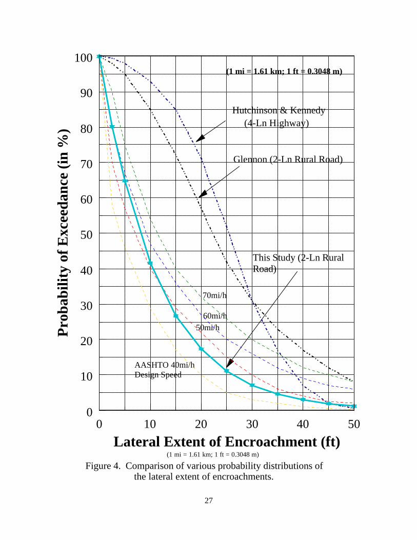
Figure 4 shows a derived probability distribution of the lateral extent of encroachments using
such approach. Since shoulder width is used to estimate the probability, the distribution is good
for leveled or flat roadside conditions with no slopes. This estimated distribution can be seen to
be quite consistent with AASHTO’s distributions for roads with a design speed of 50-60 mi/h
(80-96 km/h). On the other hand, it is very different from the distributions derived from
Hutchinson and Kennedy’s encroachment data. Note that, as pointed out by Daily et al. (5), the
basis of AASHTO's distributions is not clear from its Roadside Design Guide. In addition, the
estimation of a single distribution for a design speed has been controversial; it has been
suggested that multiple distributions for different sideslope ratios are necessary. In theory, this
distribution could be conditional on sideslope, shoulder type (e.g., paved vs. unpaved, with or
without rumble strips), density of roadside hazards, traveled path, or even encroached angle. The
readers are referred to Daily et al. (5) and Mak and Bligh (8) for more discussion. The derived
probability distribution of the lateral extent of encroachments from the proposed method can
serve as a basis to obtain more elaborated distributions under different roadside conditions.
DISCUSSIONS
The illustration above shows that the method described in this paper can be a viable approach to
estimating some of the basic encroachment parameters without actually collecting the data to
estimate them, which can be very costly. Most importantly, it is straightforward to use such an
approach to estimating basic encroachment parameters for various mainline traffic and design
conditions, e.g., AADT, lane width, horizontal curvature, and vertical grade. The only premise is
that a sound accident prediction model be developed. The better the accident prediction model,
the better the estimate of basic roadside encroachment parameters can be expected.
In theory, the proposed method can be used for road sections of roadway classes other than the
two-lane undivided roads illustrated in this paper. It is, however, not clear whether the extension
of the proposed method to consider RORA at intersections is straightforward.
Design) Rdside Other L,= SWe, MainlinL, > Encro Rdside | RORA (SV P
x ) Mainline| L > Encro Rdside ( P = Design) Rdside Other L= SW, Mainline| RORA SV( P
) Mainline|L > Encro Rdside ( P = Design) Rdside Other " Bad Extremely " L,= SW, Mainline| RORA SV( P
20
More research to explore the interrelationship between the accident-based approach and
encroachment-based approach can help develop viable and cost-effective ways of quantifying
roadside safety. The illustration provided in this paper is an example.
REFERENCES (1) Transportation Research Board. Designing Safer RoadsPractices for Resurfacing,
Restoration, and Rehabilitation. Special Report 214, TRB, National Research Council, Washington, D.C., 1987.
(2) National Highway Traffic Safety Administration (NHTSA), Traffic Safety Facts 1992, Revised, March 1994.
(3) Viner, J.G. Harmful Events in Crashes. Accident Analysis & Prevention. 25(2): 139-15; 1993.
(4) Ray, M.H., J.F. Carney III, and K.S. Opiela, Emerging Roadside Safety Issues, TR News 177, March-April, 1995.
(5) Daily, K.; W. Hughes, and H. McGee. Experimental Plans for Accident Studies of Highway Design Elements: Encroachment Accident Study. Prepared for FHWA; April 1994.
(6) Mak, K.K. and D.L. Sicking. Development of Roadside Safety Data Collection Plan, Technical Report, Texas Transportation Institute, Texas A&M University System, College Station, Texas; 1992.
(7) Viner, J.G. Rollovers on Sideslopes and Ditches. Accident Analysis & Prevention. 27(4): 483-491; 1995.
(8) Mak, K.K. and R.P. Bligh, Recovery-Area Distance Relationships for Highway Roadsides, Phase I Report, NCHRP Project G17-11, Jan. 1996.
(9) Zegeer, C.V., J. Hummer, D. Reinfurt, L. Herf, and W. Hunter. Safety Effects of Cross-Section Design for Two-Lane Roads. Volumes I and II. Chapel Hill: University of North Carolina; 1987.
(10) Zegeer, C.V., R. Stewart, D. Reinfurt, F. Council, T. Neuman, E. Hamilton, T. Miller, and W. Hunter. Cost-Effective Geometric Improvements for Safety Upgrading of Horizontal Curves. Volumes I. Final Report. Chapel Hill: University of North Carolina; 1990.
(11) Maycock, G. and R.D. Hall. Accidents at 4-arm Roundabouts. Transport and Road Research Laboratory Report 1120; 1984.
(12) Miaou, S.-P. and H. Lum. Modeling Vehicle Accidents and Highway Geometric Design Relationships. Accident Analysis and Prevention 25(6):689-709; 1993.
(13) Miaou, S.-P. The Relationship Between Truck Accidents and Geometric Design of Road Sections: Poisson Versus Negative Binomial Regressions. Accident Analysis & Prevention 26(4): 471-482; 1994.
(14) Miaou, S.-P., P.S. Hu, T. Wright, S.C. Davis, and A.K. Rathi. Development of Relationship Between Truck Accidents and Geometric Design: Phase I. Publication No. FHWA-RD-91-124, FHWA, U.S. Department of Transportation, 1993.
(15) Miaou, S.-P. Measuring the Goodness-of-Fit of Accident Prediction Models. FHWA-RD-96-040, FHWA, U.S. Department of Transportation, December 1996, 121pp.

21
(16) Glennon, J.C. Roadside Safety Improvement Programs for FreewaysA Cost Effectiveness Priority Approach. NCHRP Report 148, TRB, National Research Council, Washington, D.C., 1974.
(17) Rodgman, E., C. Zegeer, and J. Hummer. Safety Effects of Cross-Section Design for Two-Lane Roads - Data Base User's Guide, report submitted to FHWA, Revised, Nov. 1989.
(18) Miaou, S.-P., and H. Lum. Statistical Evaluation of the Effects of Highway Geometric Design on Truck Accident Involvements. In Transportation Research Record 1407, TRB, National Research Council, Washington, D.C., 1993, pp. 11-23.
(19) Hutchinson, J.W. and T.W. Kennedy. Medians of Divided HighwaysFrequency and Nature of Vehicle Encroachments. Engineering Experiment Station Bulletin 487, University of Illinois, June 1966.
(20) Cooper, P. Analysis of Roadside Encroachments Single Vehicle Run-Off-Road Accident Data Analysis for Five Provinces. B.C. Research, Vancouver, Canada, March 1980.
22
LIST OF TABLES Table 1. Estimated regression coefficients of a negative binomial regression model and associated
statistics for single -vehicle run-off-the-road accidents .......................................................23 LIST OF FIGURES Figure 1. Illustration of single -vehicle run-off-the-road accident rates for various lane widths and
sideslopes .......................................................................................................................24 Figure 2. Single-vehicle run-off-the-road accident rates for a given sideslope versus single -vehicle run-
off-the-road accident rate for a sideslope of 7:1 .................................................................25 Figure 3. Comparison of the derived roadside encroachment frequency from the accident prediction
model shown in Table 1 and observed frequencies from earlier studies ...............................26 Figure 4. Comparison of various probability distributions of the lateral extent of encroachments........27

23
Table 1. Estimated regression coefficients of a negative binomial regression model and associated statistics for single-vehicle run-off-the-road accidents.
Covariate and Parameter Estimated Parameter Value
ß1 Dummy intercept (=1)
1.20043 ("0.46;2.62)
ß2 Dummy variable for Michigan (1=Michigan; 0=otherwise)
0.6076 ("0.12;4.92)
ß3 Dummy variable for Washington (1=Washington; 0=otherwise)
0.4218 ("0.13;3.16)
ß4 AADT per lane (in 103)
-0.1783 ("0.04;-4.57)
ß5 Lane width (in ft)
-0.1411 ("0.04;-3.43)
ß6 Median clear roadside recovery distance (in ft)
-0.01375 ("0.007;-1.97)
ß7 Paved shoulder width (in ft)
ß8 Earth, grass, gravel, or stabilized shoulder width (in ft)
-0.0881 ("0.014;-6.38)
ß9 Median sideslope (e.g., 3:1 and 7:1 slopes are recorded as 1/3=0.33 & 1/7=0.14, respectively. )
0.6920 ("0.45;1.54)
ß10 Terrain type (0=flat; 1=mountainous+rolling)
0.2939 ("0.09;3.35)
ß11 Posted speed limit (in mi/h)
-----
ß12 Number of intersections per mile -----
ß13 Number of driveways per mile
0.0129 ("0.006;2.33)
ß14 Number of bridges per mile
0.2016 ("0.095;2.13)
Dispersion parameter of the NB model (a) 0.3988
("0.036;11.0)
L(a,ß) (=loglikelihood function) -1646.8
Akaike Information Criterion Value 3317.5
Expected vs. observed total number of accidents 4,709 vs 4,632 Notes: (1) 596 rural two-lane undivided road sections; total length=1,788 mi; about 5 years of accident data (1980-
1984). (2) Values in parentheses are asymptotic standard deviation and t -statistics of the coefficients above. (3) ----- indicates “not included in the model.” (4) 1 mile = 1.61 km, 1 ft = 0.3048 m.

24
Figure 1. Illustration of single-vehicle run-off-the-road accident rates for various lane widths and sideslopes.
9 10 11 12 13 40
60
80
100
120
140
160
Lane Width (in ft)
Sing
le V
ehic
le R
OR
A R
ate
7:1
2:1
Sideslope
(No.
of A
ccid
ents
/100
Mill
ion
Veh
icle
Mile
s)
(1 mi = 1.61 km; 1 ft = 0.3048 m)
AADT=1,000 Shoulder Width = 4 ft Roadside Recovery Distance =10 ft

25
Figure 2. Single-vehicle run-off-the-road accident rates for a given sideslope versus single-vehicle run-off-the-road accident rate for a sideslope of 7:1
2:1 3:1 4:1 5:1 6:1 7:1 0.9
1
1.1
1.2
1.3
1.4
Sideslope Ratio
Rat
io o
f SV
RO
RA
Rat
es
(Giv
en S
ides
lope
/Sid
eslo
pe o
f 7:1
)
(1 mi = 1.61 km; 1 ft = 0.3048 m)

26
0 5 10 15 20 25 300
1
2
3
4
5
6
7
8
9
10
11
Annual Average Daily Traffic (in 1,000s)
Kennedy and Hutchinson [1966]: Rural & Urban 4-Lane Highway, 70mi/h
Cooper [1980]: 4-Lane Highway, 50-60 mi/h
Cooper [1980]: 2-Lane Road, 50-60 mi/h
9-ft Wide Lane
10-ft
11-ft12-ft
This study : Rural 2-Lane Undivided Road55 mi/h (average of MI & WA States)
Figure 3. Comparison of the derived roadside encroachment frequency from the accidentprediction model shown in Table 1 and observed frequencies from earlier studies.
Roa
dsid
e E
ncro
achm
ent F
requ
ency
(Enc
roac
hmen
ts/M
ile/Y
ear)
(1 mi = 1.61 km; 1 ft = 0.3048 m)
SR214
(1 mi = 1.61 km; 1 ft = 0.3048 m)
27
70mi/h
60mi/h50mi/h
AASHTO 40mi/h Design Speed
Glennon (2-Ln Rural Road)
Hutchinson & Kennedy (4-Ln Highway)
Figure 4. Comparison of various probability distributions of the lateral extent of encroachments.
This Study (2-Ln Rural Road)
0 10 20 30 40 500
10
20
30
40
50
60
70
80
90
100
Lateral Extent of Encroachment (ft)
Pro
babi
lity
of E
xcee
danc
e (i
n %
)(1 mi = 1.61 km; 1 ft = 0.3048 m)
(1 mi = 1.61 km; 1 ft = 0.3048 m)


29
APPENDIX B
Working Paper
ANOTHER LOOK AT THE RELATIONSHIP BETWEEN
ACCIDENT- AND ENCROACHMENT-BASED APPROACHES TO
RUN-OFF-THE-ROAD ACCIDENTS MODELING
Shaw-Pin Miaou
Research Staff Member
Center for Transportation Analysis, Energy Division
Oak Ridge National Laboratory
P.O. Box 2008, MS 6073, Building 3156, Oak Ridge, TN 37831, USA
Phone: (423) 574-6933; Fax: (423) 574-3851; E-Mail: [email protected]
August 1997, Revised January 1998
ABSTRACT
Understanding the relationships between roadside accidents and roadside design is imperative to
developing cost-effective, road-related countermeasures to improve roadside safety. Much of what is
known today about the relationships remains to be qualitative in nature. Recent studies have suggested
that new, cost-effective analysis approaches and data collection efforts are essential if a more quantitative
basis of such relationships is to be developed. Historically, models used in previous studies to develop the
relationships have been categorized as using either an accident-based approach or an encroachment-based
approach. The former has a solid statistical ground, but has been criticized as being overly empirical and
lacking engineering basis. The latter, on the other hand, has analytical and engineering strengths, but has
been described as being full of subjective assumptions and lack of sufficient supporting data. In addition,
these two approaches seem to have been treated as two competing, disconnected approaches, and very
few attempts have been made by roadside safety researchers to combine the strengths of both. The
purpose of this study was to look for ways to combine the strengths of both approaches. The specific
objectives were (1) to present the encroachment-based approach in a more systematic and coherent way
so that its limitations and strengths can be better understood from both the statistical and engineering
30
standpoints, and (2) to apply the analytical and engineering strengths of the encroachment-based approach
to the formulation of mean functions in accident-based models.
To demonstrate the strength of mean functions so obtained, accident-based models were developed using
such mean functions for guardrail and utility pole accidents. Furthermore, to show how the accident-
based model can be useful to the encroachment-based model, the developed accident models were used to
estimate the roadside encroachment rate–a basic input parameter that is required by the encroachment-
based model and is expensive and technically difficult to collect. The estimated rates were found to be
consistent with those obtained in earlier encroachment-based studies. This is an indication that estimating
basic encroachment parameters using accident-based models can be a viable approach to reducing
encroachment data collection cost. In addition, unlike estimating encroachment parameters from the
field-collected encroachment data, the use of accident-based models to estimate encroachment parameters
does not require the development of a procedure to distinguish between controlled and uncontrolled
encroachments, which can be subjective and technically difficult to do in practice. This paper concludes
with a discussion on future research.
Key Words: Run-Off-the-Road Accident, Roadside Design, Vehicle Roadside Encroachment,
Encroachment-Based Model, Accident-Based Model
31
ANOTHER LOOK AT THE RELATIONSHIP BETWEEN ACCIDENT-
AND ENCROACHMENT-BASED APPROACHES TO RUN-OFF-THE-
ROAD ACCIDENTS MODELING
INTRODUCTION
Understanding the relationships between roadside accidents and roadside design is imperative to
developing cost-effective, road-related countermeasures to improve roadside safety. To date,
much of what is known about the relationships remains to be qualitative in nature or dependent
on subjective engineering guesses [Ray et al., 1995; Daily et al., 1997]. Recent studies suggested
that new and cost-effective analysis approaches and data collection efforts are essential if a more
quantitative basis of such relationships is to be developed [Mak and Sicking, 1992; Viner, 1995;
Mak and Bligh, 1996]. Models used in previous studies to develop the relationships between
run-off-the-road accidents (RORA) and roadside hazards, such as utility poles, trees, guardrail,
median barriers, and embankments, have been categorized as using either an accident-based
approach or an encroachment-based approach [Transportation Research Board (TRB), 1987;
Daily et al., 1997].
The accident-based approach uses statistical regression models to develop the relationships in
which the RORA frequency of hitting a particular or a combination of roadside hazards is the
dependent variable, and traffic flows, roadway mainline designs, roadside designs, and other
variables are the explanatory variables (or covariates) [Zegeer et al., 1987; Zegeer et al., 1990;
Miaou, 1996]. In the last decade or so, there has been a steady realization of the statistical
advantages of using the Poisson and negative binomial (NB) regression models over the
conventional normal distribution-based regression models when this approach is used to model
road accidents [Maycock and Hall, 1984; Miaou and Lum, 1993]. The theory behind the Poisson
and NB regression accident-based models has been discussed quite extensively in many recent
publications [e.g., Miaou, 1994; Maher and Summersgill, 1996; Miaou, 1996]. The goal of these
accident-based models is not only to estimate the expected number of accidents and its
association with key covariates, but also to estimate the statistical uncertainty associated with the
estimates. In general, these accident-based models have been developed with a solid statistical
ground.

32
Under the Poisson and NB regression models, a mean function, which is a function that relates
the mean (or expected) number of accidents to the covariates, is typically assumed to have an
exponential form. This functional form has several desirable mathematical properties and has
been widely accepted in other research areas, such as biostatistics and econometrics [Miaou,
1996]. Some of the desirable properties include: (1) it is a multiplicative function that allows
interactive effects of covariates on accidents to be easily represented; (2) it ensures that the mean
accident rate is always nonnegative; and (3) it is mathematically convenient to obtain standard
statistical inferences for the model. However, the use of such a functional form has been
criticized as being overly empirical and lacking engineering basis.
The encroachment-based approach uses a series of conditional probabilities to describe the
sequence of events resulting in a roadside accident [Glennon, 1974; TRB, 1987; Daily et al.,
1997]. A typical sequence of events considered by this approach is: (1) an errant vehicle leaves
the traveled way and encroaches on the shoulder; (2) the location of encroachment is such that
the path of travel is directed towards a potentially hazardous roadside object; (3) the hazardous
object is sufficiently close to the travel lanes that control is not regained before encounter or
collision between vehicle and object; and (4) the collision is sufficiently severe enough to result
in an accident of some level of severity. The idea of the encroachment-based approach was to
formulate and estimate these conditional probabilities based on a combination of traffic, vehicle
dynamics, and driver behavior theories. Appendix F of Transportation Research Board (TRB)
Special Report 214 (SR214) provides a good description of the concept behind the
encroachment-based approach and its application on two-lane undivided roads [TRB, 1987].
Over the last 30 years, there has been a constant effort to develop and refine the encroachment-
based models. Despite these efforts, the encroachment-based approach is still being criticized as
being full of subjective assumptions and lacking sufficient supporting data [Daily et al., 1997]. In
addition, available vehicle encroachment data, including encroachment rates, were collected on a
small number of road sections and are largely outdated. The Federal Highway Administration
(FHWA) and TRB have been addressing the requirements and collection of such data through
their sponsorship of several roadside safety projects. As a result, rather comprehensive data
collection plans have been proposed, and results of pilot data collection efforts have been
reported [Mak and Sicking, 1992; Mak and Bligh, 1996; Daily et al., 1997]. A review of these

33
plans and pilot data collection results suggests that the cost of collecting the required roadside
field data will be very high. Furthermore, the validity of any field-collected encroachment data
may be questionable because of the technical difficulty in distinguishing between controlled (or
intentional) and uncontrolled (or unintentional) encroachments.
A recent review of the encroachment-based approach and its relationship to the accident-based
approach is given in Miaou [1996]. The encroachment-based approach is appealing because of
its analytical and engineering strengths. It allows useful results from other studies, especially
those in the areas of driving behavior and vehicle dynamics, to be directly incorporated into the
model in a sensible way. In addition, systematic exploration and assessment of different road-
and vehicle-based countermeasures, which have the potential of reducing the probability of the
occurrence of each encroachment event described above, can be conducted with such an
approach. The study by Fancher et al. [1994] is an example of using the encroachment-based
approach to assess the potential benefits of using Intelligent Transportation Systems (ITS)
technologies to improve road safety.
Historically, researchers on roadside safety seem to have treated these two approaches as two
competing, disconnected approaches and seldom or never attempt to seek the opportunity to
combine the strengths of both [Mak and Sicking, 1992; Miaou, 1996]. In a recent study, Miaou
attempted to point out the complementary nature of the two approaches and suggested that the
accident-based approach can benefit from the encroachment-based thinking in obtaining a mean
function that has better engineering basis and interpretation [Miaou, 1996; Miaou, forthcoming].
Furthermore, because the data required to estimate basic encroachment parameters, such as
encroachment rates, for use in the encroachment-based model are expensive and difficult to
collect in practice, Miaou proposed a method to estimate some basic encroachment parameters
using accident-based models. The method was developed based on an exploration of the
probabilistic relationship between a roadside encroachment event and an RORA event. Miaou
illustrated the concept and use of such a method by first using data from three States, which were
contained in an FHWA Seven States Cross-Section Data Base [Rodgman et al., 1989], to
develop a RORA prediction model for rural two- lane undivided roads. The model was then used
to estimate encroachment rates by setting the clear zone width to zero and the sideslope ratio to
1:1 in the RORA prediction model.
34
The study presented in this paper is an extension of Miaou’s study [Miaou, 1996; Miaou,
forthcoming]. The purpose of this study was to look for ways to combine the strengths of both
approaches in roadside safety research. The specific objectives were (1) to present the
encroachment-based approach in a more systematic and coherent way so that its limitations and
strengths can be better understood from both statistical and engineering standpoints, and (2) to
apply the analytical and engineering strengths of the encroachment-based thinking to the
formulation of mean functions in accident-based models. To demonstrate the use of mean
functions so obtained, an accident-based model was developed using such mean functions for
guardrail and utility pole accidents from the same data base as that used by Miaou [1996].
Furthermore, to show how the accident-based model can be useful to the encroachment-based
model, similar to the approach proposed by Miaou, encroachment rates are estimated using the
developed guardrail and utility pole accident models. The rates were compared with those
estimated by Miaou [1996] and other encroachment-based studies, such as Hutchinson and
Kennedy [1966], Cooper [1980], and SR214 [1987].
This paper is organized as follows: Section 2 provides a systematic examination of the
encroachment-based thinking, addressing its limitations and strengths from both the statistical
and engineering standpoints. Section 3 describes a way to formulate mean functions for
accident-based models using encroachment-based thinking described in Section 2. Section 4
uses the formulation suggested in Section 3 to develop accident-based prediction models for
guardrail and utility pole accidents and then estimates roadside encroachment rates from these
models. This paper concludes with a discussion of future work.
The following discussion focuses on two-lane, undivided roads. However, the extension to other
roadway types should be straightforward. Also, in the discussion, a “roadside encroachment” is
said to occur when an errant vehicle crosses the outside edges of the travelway and encroaches
on either the inside or outside shoulder. Thus, for a two-lane, undivided road that has no inside
shoulder, the total number of roadside encroachments includes departures of vehicles from near-
side and far-side edges of the travelway in both directions. It is also important to note that
roadside encroachments refer only to uncontrolled (or unintent ional) encroachments. In other
words, the “controlled or intentional encroachments” resulting from vehicles intentionally driven

35
outside of the travel lane (e.g., onto shoulders and traversable medians) are not counted as
encroachments.
ENCROACHMENT-BASED THINKING
Consider a vehicle traveling through a road section of length L. The road section is characterized
by its mainline and roadside conditions. On the mainline, the condition is characterized by its
key design attributes, including lane width, horizontal curvature, and vertical grade, and by its
traffic conditions, such as traffic density and car-truck mix percentages. On the roadside, the
number and combination of various types and sizes of roadside objects, their locations along the
road section, and their lateral offsets from the edge of travelway are some of the main safety-
related characteristics of interest.
For clarity, in the following presentation, it may be necessary in some instances to indicate
which road section within the sample sections is being considered. Under such instances, we
will assume, without loss of generality, that the ith sample road section is under consideration.
Overall Concept
For a particular type of roadside object, such as guardrails or utility poles (made of the same
material), the passage that leads the subject vehicle to hit one of these objects and results in a
reportable accident is modeled as four sequential stochastic processes. Each of the four
processes is modeled by a conditional probability. Figure 1 gives an overview of these processes
and the key determinants that affect the outcome of each process. Process 1 determines the
probability that the vehicle will encroach on the roadside. If the vehicle encroaches, the
encroachment is characterized by its encroachment speed and angle, which are used as input to
Process 2. Given an encroachment speed and angle, Process 2 determines the probability that
the encroachment location of the vehicle is in a potentially hazardous envelope associated with
one of the roadside objects under consideration, which makes the impact with the object
possible. If the encroaching vehicle is in a hazard envelope, Process 3 determines whether the
vehicle will encroach far enough to collide with the object. The key output of Process 3 is an
impact speed, which can be zero (i.e., no collision). Provided that the vehicle collides with the
object, the impact speed is used as input to Process 4 to determine whether the impact will result
in a reportable accident.
36
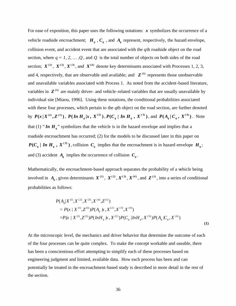
For ease of exposition, this paper uses the following notations: ξ symbolizes the occurrence of a
vehicle roadside encroachment; H q , Cq , and Aq represent, respectively, the hazard envelope,
collision event, and accident event that are associated with the qth roadside object on the road
section, where q = 1, 2, … ,Q , and Q is the total number of objects on both sides of the road
section; X ( )1 , X ( )2 , X ( )3 , and X ( )4 denote key determinants associated with Processes 1, 2, 3,
and 4, respectively, that are observable and available; and Z ( )1 represents those unobservable
and unavailable variables associated with Process 1. As noted from the accident-based literature,
variables in Z ( )1 are mainly driver- and vehicle-related variables that are usually unavailable by
individual site [Miaou, 1996]. Using these notations, the conditional probabilities associated
with these four processes, which pertain to the qth object on the road section, are further denoted
by P X Z( | , )( ) ( )ξ 1 1 , P In H Xq( | , )( )ξ 2 , P C In H Xq q( | , )( )3 , and P A C Xq q( | , )( )4 . Note
that (1) “ In H q ” symbolizes that the vehicle is in the hazard envelope and implies that a
roadside encroachment has occurred; (2) for the models to be discussed later in this paper on
P C In H Xq q( | , )( )3 , collision Cq implies that the encroachment is in hazard envelope H q ;
and (3) accident Aq implies the occurrence of collision Cq .
Mathematically, the encroachment-based approach separates the probability of a vehicle being
involved in Aq , given determinants X ( )1 , X ( )2 , X ( )3 , X ( )4 , and Z ( )1 , into a series of conditional
probabilities as follows:
),|(),|(),|(),|(
),,,|(),|(
),,,,|(
)4()3()2()1()1(
)4()3()2()1()1(
)1()4()3()2()1(
XCAPXHInCPXHInPZXP
XXXAPZXP
ZXXXXAP
qqqqq
q
q
ξξ
ξξ
=
=
(1)
At the microscopic level, the mechanics and driver behavior that determine the outcome of each
of the four processes can be quite complex. To make the concept workable and useable, there
has been a conscientious effort attempting to simplify each of these processes based on
engineering judgment and limited, available data. How each process has been and can
potentially be treated in the encroachment-based study is described in more detail in the rest of
the section.
37
Process 1
One of the efforts made to simplify the analytical procedure is to separate Process 1 from the rest
of the processes. This is done by introducing the assumption that roadside design has a
negligible effect on roadside encroachment probability. In other words, this assumption says that
the probability of encroachments can be solely determined from mainline conditions. This
assumption simplifies the analytical procedure significantly. Specifically, it allows the analysts
to stay focused on the analysis of the last three processes, which pertain to the effect of
alternative roadside designs on the accident probability, without worrying about the roadside
encroachment rates and characteristics being altered as a result of different roadside designs.
However, the validity of this assumption has not been formally challenged and may be debatable.
For example, some may believe that some roadside conditions, such as a sharp sideslope, can
significantly affect a driver’s driving behavior (e.g., driver’s attentiveness) and therefore affect
roadside encroachment rates.
Using this assumption, previous encroachment-based studies typically started the analysis with
the premise that data on encroachment rates and two key encroachment characteristics, namely,
encroachment speed and angle, are available either from some data collection efforts or can be
pre-estimated. Encroachment rates, angles, and speeds are, however, expected to vary by
weather condition, roadway functional class, average annual daily traffic (AADT), lane width,
horizontal curvature, vertical grade, and even car-truck mix percentage [Mak and Sicking, 1992].
Thus, besides the potential technical difficulties to be discussed next, the effort required to
collect a comprehensive set of encroachment data under all these conditions will be tremendous.
Many data collection instruments have been used to obtain roadside encroachment data,
including observing tire-tracks, monitoring maintenance records of roadside objects, and using
electronic monitoring equipment such as video cameras [Mak and Sicking, 1992; Daily et al.,
1997]. However, so far, most of the data collection efforts have been small-scale and
experimental in nature and were not considered successful. As indicated earlier, even if the
controlled encroachments can be distinguished from the uncontrolled encroachments, the effort
required to collect all of the necessary data is expected to be expensive. One additional note
regarding controlled and uncontrolled encroachments is that no formal, quantitative definitions
of them exist. Recognizing that oftentimes there is a fine line between a controlled and an
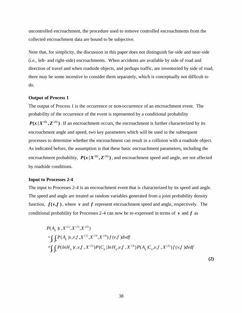
38
uncontrolled encroachment, the procedure used to remove controlled encroachments from the
collected encroachment data are bound to be subjective.
Note that, for simplicity, the discussion in this paper does not distinguish far-side and near-side
(i.e., left- and right-side) encroachments. When accidents are available by side of road and
direction of travel and when roadside objects, and perhaps traffic, are inventoried by side of road,
there may be some incentive to consider them separately, which is conceptually not difficult to
do.
Output of Process 1
The output of Process 1 is the occurrence or non-occurrence of an encroachment event. The
probability of the occurrence of the event is represented by a conditional probability
P X Z( | , )( ) ( )ξ 1 1 . If an encroachment occurs, the encroachment is further characterized by its
encroachment angle and speed, two key parameters which will be used in the subsequent
processes to determine whether the encroachment can result in a collision with a roadside object.
As indicated before, the assumption is that these basic encroachment parameters, including the
encroachment probability, P X Z( | , )( ) ( )ξ 1 1 , and encroachment speed and angle, are not affected
by roadside conditions.
Input to Processes 2-4
The input to Processes 2-4 is an encroachment event that is characterized by its speed and angle.
The speed and angle are treated as random variables generated from a joint probability density
function, f v( , )φ , where v and φ represent encroachment speed and angle, respectively. The
conditional probability for Processes 2-4 can now be re-expressed in terms of v and φ as
∫ ∫∫ ∫
=
=
φ
φ
φφφφφξ
φφφξ
ξ
v qqqqq
v q
q
ddvvfXvCAPXvHInCPXvHInP
ddvvfXXXvAP
XXXAP
),(),,,|(),,,|(),,,|(
),(),,,,,|(
),,,|(
)4()3()2(
)4()3()2(
)4()3()2(
(2)
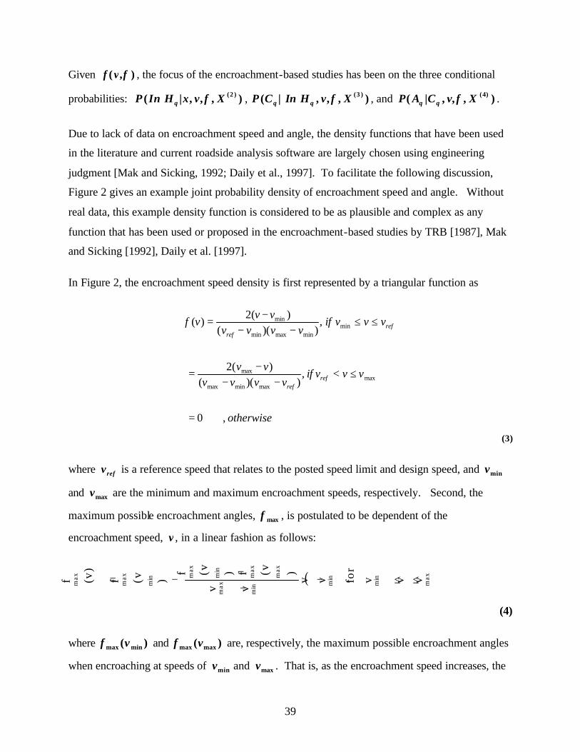
39
Given f v( , )φ , the focus of the encroachment-based studies has been on the three conditional
probabilities: P In H v Xq( | , , , )( )ξ φ 2 , P C In H v Xq q( | , , , )( )φ 3 , and P A C v Xq q( | , , , )( )φ 4 .
Due to lack of data on encroachment speed and angle, the density functions that have been used
in the literature and current roadside analysis software are largely chosen using engineering
judgment [Mak and Sicking, 1992; Daily et al., 1997]. To facilitate the following discussion,
Figure 2 gives an example joint probability density of encroachment speed and angle. Without
real data, this example density function is considered to be as plausible and complex as any
function that has been used or proposed in the encroachment-based studies by TRB [1987], Mak
and Sicking [1992], Daily et al. [1997].
In Figure 2, the encroachment speed density is first represented by a triangular function as
otherwise
vvvifvvvv
vv
vvvifvvvv
vvvf
refref
refref
,0
,))((
)(2
,))((
)(2)(
maxmaxminmax
max
minminmaxmin
min
=
≤<−−
−=
≤≤−−
−=
(3)
where vref is a reference speed that relates to the posted speed limit and design speed, and vmin
and vmax are the minimum and maximum encroachment speeds, respectively. Second, the
maximum possible encroachment angles, φmax , is postulated to be dependent of the
encroachment speed, v , in a linear fashion as follows:
( ) max
min
min
min
max
max
max
min
max
min
max
max vvvfo
r,vv
vv
)(vf)(vf
)(vf(v)
f ≤≤−
−−
−=
(4)
where φmax min( )v and φmax max( )v are, respectively, the maximum possible encroachment angles
when encroaching at speeds of vmin and vmax . That is, as the encroachment speed increases, the

40
possible encroachment angle decreases in a linear fashion. This relationship is based on the
notion that most vehicles do not rollover at the time of encroachment. That is, the roadholding
capacity that a vehicle can provide is not exceeded at the outset of most of the encroachments.
Third, the probability density of the encroachment angle φ , given φmax , is represented by
another triangular function as
0
,12
)|( maxminminmax
min
minmaxmax
=
≤≤
−
−−
−= φφφ
φφφφ
φφφφ iff
(5)
Note that, mathematically, it is straightforward to combine all three equations into a joint density
function by using the relationship
)()|()()|(),(
max vffvfvfvf
φφφφ
==
(6)
However, this mathematical expression is quite complicated and will not be presented here. An
obvious deficiency of this joint density function is that it ignores the effect of horizontal
curvatures on φ .
To have some understanding of the statistical properties of the exemplified joint density function,
a Monte-Carlo simulation was performed with the following parameter values: vmin=0, vref =55
mi/hr, vmax =70 mi/hr, φmax min( )v =40o, φmax max( )v =15o, and φmin =0.25o. The reason why
φmin =0.25o is used, instead of 0o, will be given later. The simulation results show that the
expected value of encroachment speed, expressed as [ ]E v , is 41.7 mi/hr, and the unconditional
expectations [ ]E φ and [ ]E φmax are, respectively, equal to 8.5o and 25.1o. Note that the same
set of parameter values for the joint density function, f v( , )φ , was used for all of the Monte-
Carlo simulations performed in this study.

41
Process 2
Process 2 determines P In H v Xq( | , , , )( )ξ φ 2 for each of the Q objects. Figure 3 shows a
commonly used formula to compute the size of the hazard envelope, given φ , vehicle swath
width (Wveh), and length and width of the considered object (l obj q, and Wobj q, ). This is
expressed as
)csc()cot(,,, φφ vehqobjqobjqenv WW ++= ll
(7)
This formula has been widely used and discussed [TRB, 1987; Daily et al., 1997]. It is based on
the assumption that the road section is a straight section with no horizontal curvature and that the
trajectory of the encroaching vehicle is a straight line.
Hazard envelopes can, of course, overlap when multiple objects exist and are located closely to
one another. This is especially true when φ is small. By considering the potential for
overlapping of H q , the conditional probability can be expressed as
LOLWW
LOL
XXv
qvehqobjqobj
qqenvqq
2)8()()csc()cot(
2)(
),,|HP(In ),,,|HP(In
,,
,)2()2(
φφφ
φφξφξ
−++=
−==
l
l
(8)
where L is the length of the road section, and OLq ( )φ represents an adjustment of the size of
H q that is overlapped by other objects and is a function of φ . The use of 2L in the
denominator requires the assumption that encroachments are equally likely to occur on the right
and left sides of the road, and that the encroachment is equally likely to occur at any location
within the road section. These assumptions are good only for a straight and level road section
that is homogeneous in traffic and design variables, such as AADT and lane width, within the
road section.

42
Estimating the size of overlapping envelopes can be a tedious bookkeeping process and is
usually avoided in the modeling stage by either selecting objects that are typically far away from
one another or by treating closely located objects as one continuous object [TRB, 1987; Daily et
al., 1997; Rodgman et al., 1989]. Another potential problem with estimating the H q , which is
usually ignored, is that the envelope of those objects that are located close to the end points of
the road section can have significant part of the envelope falling on adjacent sections. Of course,
adjacent sections may have envelopes falling on the section under consideration. If the objects
are evenly located across the section, this “boundary problem” will roughly cancel out.
Otherwise, more tedious bookkeeping procedures may be required.
In practice, when a type of point object is considered, qobj,l and qobj,W are usually set to
constants for all Q objects. In addition, when a round-shaped object is considered, it is typically
treated as a squared object and l obj q, and Wobj q, are set approximately equal to the diameter of
the object. For example, for utility poles, l obj q, = Wobj q, = 8 inches have been used [TRB,
1987]. For a particular type of continuous object considered, such as guardrails, the length l obj q,
varies over q, but Wobj q, remains fairly constant for all objects. Also, Wveh is fixed and
determined with a design vehicle (e.g., a mid-sized car) in mind. For example, Wveh was set to 6
ft in SR214 and to 12 ft in Roadside Design Guide [American Association of State Highway and
Transportation Officials (AASHTO), 1989]. Note that, for the point object, the size of the
hazard envelope, as calculated in Eq. (7), is dominated by the term Wveh csc( )φ because Wveh is
considerably larger than l obj q, and Wobj q, . On the other hand, for the continuous object, l obj q, is
usually the dominant term in Eq. (7).
To gain some understanding of the size of H q , two Monte-Carlo simulations were conducted
with the same joint density f v( , )φ as in the previous simulation and with Wveh set to 9 ft. The
first simulation is intended to represent the size of H q for a long guardrail with l obj q, =1,320 ft
(or 0.25 mi) and Wobj q, =1 ft. The simulation results show that the minimum, average, and
maximum sizes of the envelopes are about 1,336 ft, 1,493 ft, and 3,610 ft, respectively. (Note
that the average size of the envelope is a simulation-based estimate of the integral

43
[ ]l obj q obj q vehvW W f v dv d, , cot( ) csc( ) ( , )+ +∫∫ φ φ φ φ
φ). In this simulation, on average,
W Wveh objcsc( ) cot( )φ φ+ = 173 ft, in which Wveh csc( )φ =156 ft and Wobj cot( )φ =17 ft. This
suggests that, for a short continuous object, e.g., l obj q, < 500 ft, the proportion of the envelope
that is attributed to vehicle swath width and object width may not be ignored. This is mainly
because φ is typically small (for straight road sections), which makes csc( )φ and cot( )φ large.
The second simulation run was performed to represent the envelope of a utility pole that was
assumed to have an 8- inch diameter. The corresponding minimum, average, and maximum sizes
of the envelope are 16 ft, 168 ft, and 2,214 ft, respectively. In this simulation, on average,
Wveh csc( )φ =156 ft and Wobj cot( )φ =12 ft. This suggests that, even with a relatively small
point object like a utility pole, the size of the envelope can be very wide due, again, to vehicle
swath width and object width, as a result of small encroachment angles. These two simulations
indicate that l obj L2 will not be a good approximation of the conditional probability in Eq. (8)
in practice when point objects are considered and may not be good for continuous objects when
the length of the object is short.
Note that the average sizes of Wveh csc( )φ and Wobj cot( )φ obtained from this utility pole
simulation is considerably larger than, for example, that obtained by Hutchinson and Kennedy
[1966] and that used in Roadside Design Guide [AASHTO, 1989]. In Hutchinson and Kennedy,
a near-side encroachment angle of 6.1o and a far-side encroachment angle of 11.5o were
estimated from limited encroachment data. These angles were used to compute the average size
of the envelope using Eq. (7). Assuming that two-thirds of the encroachments are near-side
encroachments and one-third are far-side encroachments, this gives an average encroachment
angle of about 8o. Now, using the same vehicle swath width of 9 ft as in the simulation, we have
W Wveh objcsc( ) cot( )φ φ+ = 64.7 ft + 4.7 ft = 69.4 ft. In Roadside Design Guide, an
encroachment angle of 15.2o is recommended for both near-side and far-side encroachments. The
basis of this recommendation is, however, not clear. Nevertheless, under this recommendation
and using the same vehicle swath width, W Wveh objcsc( ) cot( )φ φ+ = 34.3 ft + 2.5 ft = 36.8 ft.
Thus, assuming that the vehicle swath width of 9 ft can be agreed on, the size of
44
W Wveh objcsc( ) cot( )φ φ+ obtained from the utility pole simulation in this study is, respectively,
about 2.4 and 4.5 times that used by Hutchinson and Kennedy [1966] and Roadside Design
Guide [1989]. Unfortunately, there is no good supporting data to judge the validity of any of
these estimates.
One may have noticed that, in the two examples above, a single encroachment angle is used to
estimate the expected size of the hazard envelope with Eq. (7), instead of using the entire
distribution of the encroachment angle. This has been practiced by many studies, e.g., SR214
[TRB, 1987] and Daily et al. [1997]. This poses an important question as to what a good cho ice
of φ value would be if one is to choose one value to estimate the average or expected size of H q
using Eq. (7). One observation made from the simulations above was that, when l obj q, is short,
plugging- in the average encroachment angle in Eq. (7) is not a good estimate of the average size
of envelope. For example, in the guardrail example, if one uses the average angle 8.5o in Eq. (7),
the average size of the envelope would be estimated as 1,387 ft (which is about 7 percent lower
than the actual average envelope (1,493 ft) estimated from the simulation. However, in the
utility pole example, the estimate would be 66 ft, which is about 60 percent lower than the actual
average envelope of 168 ft. The reason for the underestimation is that the distribution of φ is
skewed to the right (with a positive coefficient of skewness) and the size of the envelope is a
nonlinear function of φ . If the average encroachment angle is not a good choice, what φ value
should be used to estimate the expected size of H q using Eq. (7)? This particular question did
not seem to be addressed by earlier studies when estimating the size of the envelope for point
objects, such as sign posts and utility poles [TRB, 1987; Daily et al., 1997]. The validity of
these practices is, therefore, questionable.
Note that the expected size of H q , which is represented analytically as
[ ]l obj q obj q vehv
vvW W f v dv d, ,
( )cot( ) csc( ) ( , )
min
max
min
max+ +∫∫ φ φ φ φ
φ
φ, does not exist if φmin =0. This is
the reason φmin =0.25o was used instead of 0o in previous simulations. The choice of φmin =0.25o
is arbitrary; it is simply chosen to represent a very small encroachment angle.
Process 3

45
Process 3 determines P C In H v Xq q( | , , , )( )φ 3 , the probability that if the vehicle encroaches
and is in H q , the vehicle will collide with the object. As indicated in Figure 1, many factors are
involved in this process, including roadside, vehicle, and driver conditions. The main roadside
conditions that have been considered in the encroachment-based studies are lateral offset of the
object, Dobj , and surface type, slope, and wetness. These determinants are also recognized as the
key roadside variables by the accident-based studies [Zegeer et al., 1987; Zegeer et al., 1990;
Miaou, 1996]. It is obvious that Dobj can vary from object to object, which will therefore be
denoted by Dobj q, . The main vehicle conditions identified by the encroachment-based studies
include vehicle braking system and tire condition, while the main driver variables identified
include the driver’s response delay (to the occurrence of roadside encroachment) and the driver’s
braking and steering behavior after the vehicle encroaches. As mentioned earlier, this is the
process where research results in vehicle dynamics and driver behavior (including maneuvering
characteristics and in-vehicle habits) can potentially be incorporated. For example, the Highway
Vehicle Object Simulation Model is a sophisticated vehicle-handling simulation model that has
been used in some encroachment-based studies [Mak and Sicking, 1992; Mak and Bligh, 1996].
Note that, depending on the focus of the study, the choice of the level of analytical complexity
for modeling this process is oftentimes at the discretion of the analysts.
To illustrate the concept, simple kinematic equations will be presented here. These equations
have been used to estimate time to collision and impact speed for a given encroachment speed
and angle with the assumptions that encroachment trajectory is a straight line and deceleration
rate is a constant [Mak and Sicking, 1992]. Table 1 shows these equations under different
encroachment conditions. In these equations, the lateral offset, Dobj , is the key roadside variable
that is explicitly modeled, while surface type, slope, and wetness are implicitly modeled through
the choice of vehicle deceleration rate ( ∆ ). Vehicle braking system and tire condition are also
implicitly represented via the choice of ∆ . Driver response delay, t r , is explicitly considered,
while braking behavior is remotely implied in the choice of ∆ . Steering behavior, on the other
hand, is ignored completely. Despite their simplicity, these equations do capture a simple crash-
avoidance maneuver very well at the conceptual level and can serve as a basis for considering
more complicated maneuvers.
46
In theory, one can choose t r from a distribution function that represents the probability of a
driver’s response delay in typical roadside encroachment circumstances due to the driver’s
temporary inattentiveness, as well as in extreme cases where a driver falls asleep completely.
The data to calibrate this distribution function are, however, not available and have not been
considered in the data collection plans mentioned earlier.
It is worth pointing out that ignoring a driver’s ability to make steering correction is a critical
limitation, since most of the encroachments are expected to have small encroachment angles and,
under such encroachments, the alerted driver can usually apply a combination of braking and
steering operations to swerve the vehicle back into the travel lane before hitting any object.
Clearly, the effects of many factors are being lumped together and implied in a simple variable,
∆ . Without additional modeling effort, it will be difficult, and possibly meaningless, to suggest
a probability distribution function for ∆ . Intuitively, ∆ is highly dependent on the roadside
surface condition, especially sideslope ratio, which is of great interest to this study. By limiting
the choice of ∆ to a constant, one can at best assume some sort of ideal braking and roadside
surface conditions.
Since a straight-line trajectory is assumed above, the impact angle is the same as the
encroachment angle. More complicated trajectories and vehicle yaw rates can, of course, be
considered in the process so that a collision is characterized not only by its impact speed, but also
by its angle and position of impact. Again, the data to support these more complicated scenarios
are either extremely limited or not available.
Given that an encroached vehicle is in the envelope of an object, additional simulations were
conducted to illustrate the conditional probability using the kinematic equations in Table 1. In
these simulations, new parameters were set: t r =1 sec and ∆ =0.5 g =16.1 ft/sec2. These
parameters represent an alerted driver and a car encroaching on a relatively flat surface with a
good tire-surface friction coefficient. Lateral offsets, Dobj , are set for 0, 5, 10, 15, 20, …, 50 ft at
different simulation runs. Given v , φ , constants t r and ∆ , and the encroachment location within
H q , the impact speed associated with the qth object, Vc q, , can be computed deterministically
using the equations in Table 1. Figure 4 shows the distribution of impact speeds as a result of
47
different encroaching speeds, angles, and locations within H q . Analytically, Figure 4 shows the
collision probability P C In H X P C In H v X f v dv dq q q qv( | , ) ( | , , , ) ( , )( ) ( )3 3= ∫∫φ
φ φ φ .
Figure 4(a) shows that the percentage of vehicles that hit the object decreases as the lateral offset
of the object increases. For those that impact the object, Figure 4(b) further shows the
distributions of their impact speed for different lateral offsets of the object. It was noted that the
rate of decrease in collision probability in Figure 4(a) is almost a constant, but it is not as
pronounced as those used in the current Roadside Design Guide and that estimated in Miaou
[AASHTO, 1989; Miaou, 1996; Miaou, forthcoming]. Note that Miaou assumed an exponential
rate of decrease for a roadside surface that is relatively flat and showed that the results are quite
consistent with those used in the Roadside Design Guide [AASHTO, 1989; Miaou, 1996]. Of
course, there are many possible explanations for their discrepancies, such as the simplification of
behavior models in the simple kinematic equations.
Combining Processes 2 and 3
Both Processes 2 and 3 are conditional on v and φ . To understand the analytical property of
these two processes jointly, Monte-Carlo simulations were conducted for different sizes of point
objects and for various lengths of continuous objects. Mathematically, the simulation seeks to
understand the following process:
∫ ∫∫ ∫
=
=
φ
φ
φφφφξ
φφφξξ
v qqq
v qq
ddvvfXvHInCPXHInP
ddvvfXXvCPXXCP
),(),,,|(),,|(
),(),,,,|(),,|(
)3()2(
)3()2()3()2(
(9)
Eq. (8) and the simple kinematic equations in Table 1 are used in the simulation. Again, the
simulations were conducted for different lateral offsets of the object. The length of the road
section is fixed and set to L = 1 mi (5,280 ft ).
For the simulations of point objects, two round-shaped objects of the same lateral offset, one on
each side of the road, are considered. The simulations were conducted for various sizes of the
object, ranging from 4 inches to 12 inches in diameter. Figure 5 shows the collision probabilities
by lateral offsets and by size of the object. Figure 5(a) shows that the probability decreases

48
monotonously as the lateral offset increases. Additional computations revealed that the
percentage decrease in collision probability is not a constant; it decreases drastically initially and
becomes a constant as the lateral offset increases. This suggests that, for a particular type of
point object considered (of the same size), an exponential function of the lateral offset is a good
candidate function to represent the collision probability. However, within the exponential
function, the coefficient associated with the lateral offset may have to change as the lateral offset
increases. Thus, within the exponential function, either a second or higher order polynomial
function or a step function of the lateral offset (which will be described in the next section) may
have to be considered. Figure 5(b) indicates that, for a fixed lateral offset, the probability of a
collision increases in a linear fashion as the size of the object increases. More specifically, the
probability of a collision increases in a linear fashion as the average size of the hazard envelope
increases (not shown in the figure).
For the simulations of continuous objects, two objects of the same lateral offset, one on each side
of the road, are again considered. The widths of the objects are set to a constant (Wobj q, =1 ft)
and length l obj q, varies from 100 ft to 2,500 ft. Figure 6 shows the same probabilities as those
presented for the point objects. Figure 6(a) shows that the probability of a collision decreases as
the lateral offset increases. As in the point object simulations, an exponential function of the
lateral offset is a good candidate function to represent the collision probability. An interesting
observation is that, for l obj q, ≥ 750 ft, the rate of decrease in collision probability appears to be
fairly constant as the lateral offset increases. This suggests that, within the exponential function,
a simple linear function of the lateral offset with one coefficient will be suffice for representing
the collision probability when l obj q, ≥ 750 ft. As the length of the object becomes shorter
(relative to 750 ft), the percentage decrease in collision probability deviates further from a
constant. And, as the length becomes very small, the percentage decrease in collision probability
decreases drastically initially and becomes a constant as the lateral offset increases. As in the
point object, to model the collision probability for short continuous objects, a second or higher
order polynomial function or a step function of the lateral offset becomes necessary within the
exponential function. Also, Figure 6(b) indicates that, for a fixed lateral offset, the probability of
a collision increases in a linear fashion as the size of the object (or, more precisely, the size of
hazard envelope) increases.
49
Output of Process 3
One of the key outputs from Process 3 is an impact speed. If the impact speed is greater than
zero (i.e., an object is hit), then it serves as input to Process 4.
Process 4
Process 4 determines P A C v Xq q( | , , , )( )φ 4 . As mentioned earlier, in a more sophisticated
vehicle trajectory model, the collision is characterized by impact speed, impact angle, and the
position of impact. However, in previous studies, very simple conditional probabilities have
been assumed based on limited data and some engineering judgment. For example, a constant
probability of 0.9 was used for hitting utility poles in SR214. A more sensible way would be to
determine the probability based on the impact speed (or the lateral offsets of objects since the
impact speed is a function of lateral offsets). For simplicity, the impact speed is the only
collision characteristics considered in this study. To make the impact speed explicit in the
conditional probability, we can write P A C V Xq q c q( | , ), ,( )4 , instead of P A C v Xq q( | , , , )( )φ 4 .
This probability has to be determined for each type of object. For example, it may be decided
that if the impact speed with a utility pole is greater than 5 mph, then it will result in a reportable
accident. That is,
P A C V X Vq q c q c q( | , ), ,( )
,4 = > 1 if 5 mi / hr (10)
= 0 otherwise
The choice of the threshold impact speed is, of course, dependent on the nature of the object
considered (e.g., the material of which the object is made).
Similar to the setup of the last simulations, a simulation was conducted to gain some
understanding of the probability when different thresholds of Vc q, are chosen. Figure 7 shows
the probabilities for an 8- inch diameter point object and a 0.25-mile continuous object.
Naturally, the probability decreases as a higher threshold value of Vc q, is chosen. However, the
simulation results suggest that the decrease in probability is very small when Vc q, increases from
0 to 10 mi/hr. Another interesting observation is that, for a given threshold value of Vc q, , the
decrease in collision probability remains very much the same as the lateral offset increases.

50
The severity of accidents is expected to be some function of impact speed. Therefore, this is the
process where the conditional probability of various accident severity levels could potentially be
considered. Conceivably, crash test results, which can be computer simulated, can potentially
be used to determine the relationship between severity and impact speed. Also, this is the
process where the changes of safety features in vehicle population can be reflected, such as the
percentages of vehicles equipped with airbags and dynamic side- impact protection and the rate
of seat-belt use.
Overall Probability and Expected Number of Accidents
Provided that the overlapping of H q can be properly accounted for (or avoided), the probability
of an encroached vehicle to be involved in an accident with one of the objects on the road,
symbolized by A , is the sum of the probability over all objects:
∑ ∫ ∫
∑ ∫ ∫
=
=
=
=
Q
qv qqqqq
Q
qv q
ddvvfXvCAPXvHInCPXvHInP
ddvvfXXXvAP
XXXAP
1
)4()3()2(
1
)4()3()2(
)4()3()2(
),(),,,|(),,,|(),,,|(
),(),,,,,|(
),,,|(
φ
φ
φφφφφξ
φφφξ
ξ
(11)
As stated earlier, in the encroachment-based studies, it is expected that the (expected)
encroachment rate can be pre-determined based on mainline conditions. The encroachment rate,
denoted by Rξ , is typically given as the number of encroachments per million vehicle-miles
traveled. Given Rξ and all determinants, the expected number of accidents on the road section
in N years is calculated as
( ) ),,,|(10/365
],,,,|[)4()3()2(6
)4()3()2()1()1(
XXXAPRLAADTN
XXXZXYE
ξξ ×××××
=
(12)
where Y is the number of reportable accidents involving the type of objects, L is in miles, AADT
is in number of vehicles, and ( )365 106× × × ×N AADT L R/ ξ is the expected total number of
encroachments during the period. One of the basic encroachment parameters of interest is the
51
expected encroachment frequency per mile per year. If Rξ is estimated and symbolized as $Rξ ,
then the encroachment frequency can be obtained as ( )365 10 6× ×AADT R/ $ξ . An implicit
assumption used here is that the RORA experiences of individual drivers traveling through the
section are independent from one another (which is a reasonable one).
FORM OF MEAN FUNCTIONS
Unlike the encroachment-based approach, the accident-based approach deals with one
conditional probability only: the probability of having y accidents, given the available
determinants, or mathematically, P Y y X Z X X X( | , , , , )( ) ( ) ( ) ( ) ( )= 1 1 2 3 4 , where y = ∞1 2 3, , , . . , .
There are basically five major tasks in developing accident-based models: (1) find a good
probability (mass) function to describe the random variation of accident frequency; (2) determine
an appropriate functional form and parameterization for the mean function which describes the
effect of key variables on accident frequency; (3) select the variables that have statistically
significant effects on accident frequency for inclusion in the mean function; (4) estimate the
regression parameters in the mean function and obtain good statistical inferences for the
estimated parameters based on available data; and (5) assess the quality of the model; judge
whether the developed model makes good engineering sense; decide whether the developed
model meets the planning and design requirements; and identify cost-effective ways to improve
the model. The work involved in each of these tasks has been described in Miaou [1996]. Since
the theory behind the Poisson and NB regression accident-based models have been discussed
quite extensively in many recent publications [Maycock and Hall, 1984; Miaou et al., 1993;
Miaou and Lum, 1993; Miaou, 1994; Maher and Summersgill, 1996; Miaou, 1996], the readers
are referred to these publications for a review of these models.
As seen in the last section, the focus of the encroachment-based model has been on the second
task, determining the appropriate functional form and parameterization for the mean function and
on identifying key determinants. In this section, several mean functions will be formulated for
use in the accident-based models, following the encroachment-based thinking described in the
last section. Specifically, the objective is to determine mean functions based on Eqs. (11) and
(12) and simulation experience gained in the last section.

52
As stated earlier, the encroachment-based thinking described above does not provide any
engineering insights on what the plausible functional forms of P X Z( | , )( ) ( )ξ 1 1 might be. Thus,
it does not provide any clue as to the functional form of Rξ in relation to X ( )1 and Z ( )1 . It has
been argued in the accident-based literature that a plausible functional form should be
mutiplicative in nature and represent the interactive effects of various mainline design and traffic
variables on accident frequency. The exponential form has been suggested to be a good
candidate because it is simple and it ensures that the expected value will always be non-negative
[Miaou, 1996]. By applying the same argument to the encroachment frequency, we can express
the encroachment rate as
)exp(2
*1 ∑∑ ++=
= kikk
jijj zxR γββξ
(13)
where, for clarity, the subscript i introduced to represent the road section being considered is the
ith section in the sample road sections; x ij is the value of the available mainline design and
traffic variables for the ith road section; zik is the value of the unobservable variables for the
section; and β1* , β ’s, and γ ’s are unknown model parameters. Note that, when appropriate,
higher order and interactive terms of the covariates can be easily included in Eq. (13).
The encroachment-based thinking described in the last section does provide some good ideas on
the choice of the functional from in Eq. (11). One such choice, which is consistent with the
simulation results shown in Figures 5-7, would be
[ ]P A W DL
D D Dobj obj objobj q q
obj q obj q obj qq
Q
v( | , ) exp( . . . ) ( ),,
, ,( )
,( )l
l=
+
+ + +
=∑
δα α α η
2141 2
13
2
1
where δq is the part of the hazard envelope associated with vehicle swath width, object width,
and adjustments for the overlapping of envelopes; a polynomial or a step function of Dobj q, is
used within the exponential function to model collision probabilities (as suggested from the
previous simulations); α ’s are unknown parameters associated with the polynomial function;
and ηv is associated with the threshold impact speed discussed earlier and is a constant between

53
0 and 1. When ηv =1, it indicates that any impact speed greater than 0 will result in an accident.
According to the simulation results shown in Figure 7, ηv should be fairly close to 1 if the
threshold impact speed is less than 10 mi/hr. Thus, for typical non-breakaway, fixed objects, if
we are interested in all reportable accidents (regardless of their severity) a reasonably good
estimate of ηv would be close to 1 and can be determined outside of the accident model.
Note that, to use a polynomial function of Dobj q, in Eq. (14), Dobj q,( )1 = Dobj q,
2 , Dobj q,( )2 = Dobj q,
3 , and
Dobj q,( )3 = Dobj q,
4 , etc., and, for a step function, Dobj q,( )1 = Dobj q, , if Dobj q, is greater than a
predetermined distance, e.g., 5 ft, otherwise a zero is assigned; Dobj q,( )2 = Dobj q, , if Dobj q, is greater
than a larger predetermined distance, e.g., 10 ft, otherwise a zero is assigned; and Dobj q,( )3 = Dobj q, , if
Dobj q, is greater than another larger predetermined distance, e.g., 15 ft, otherwise a zero is
assigned, etc. The step function so arranged would allow the rate of decrease in collision
probability to change in a step-wise manner as the lateral offset increases. For the example step
function here, the percent decrease in collision probability is approximately − 100 1α % per foot
increase in Dobj q, when Dobj q, is between 0 and 5 ft, − +100 1 2( )%α α when Dobj q, is between 5
and 10 ft, and − + +100 1 2 3( )%α α α when Dobj q, is between 10 and 15 ft, etc.
In Eq. (14), Dobj q, is the only roadside design variable considered in determining collision
probability after roadside encroachments occur. As indicated earlier, sideslope and surface types
are two other key variables that were implicitly considered in the simulations presented earlier.
Thus, a plausible extension of Eq. (14) is to add sideslope as the second roadside design variable
within the exponential function on the right-hand side of Eq. (14). However, a representative
sideslope may be difficult to obtain for two reasons: (1) the sideslope can vary significantly
within a road section, and (2) for a particular object, the sideslopes of interest are the slopes that
are located within the hazard envelope of the object, the location and size of which also need to
be estimated. Also, to reflect the difference in the friction coefficient of different surface types,
such as paved and unpaved shoulders, in the model, the lateral offset, Dobj q, , can be provided by
surface type and the model parameter associated with the lateral offset can vary from one surface
type to another.

54
Substituting Eqs. (13) and (14) into Eq. (12), we have a general mean function for the accident-
based models for both point and continuous objects.
( )
[ ] (16)
+++
+×
+××××
=
∑
∑
=
=
vqobjqobjqobj
Q
q
qqobj
jijj
DDDL
xLAADTN
XXXXYE
ηαααδ
ββ
...)exp(2
)exp(10/365
],,,|[
)2(,3
)1(,2,1
1
,
21
6
)4()3()2()1(
l
where α ’s, β ’s and γ ’s are unknown model parameters to be estimated from the data. It
should be noted that the term exp( )γ k ikkz∑ has been taken out of the expectation since the
variable Z ( )1 is not available in practice. Using the Poisson assumption for the randomness of
accident frequency, together with the assumption that the exponential function of the
unobservable variables (i.e., exp( )γ k ikkZ∑ ) is gamma distributed with an expected value of
one, a negative binomial regression model can be derived with Eq. (16) as its mean function
[Miaou, 1996]. These two assumptions are quite plausible and flexible for count data analysis.
They have been used in accident-based models and widely accepted in other fields such as
biostatistics and econometrics.
In Eq. (16), δq is a variable that varies over individual object. If overlapping of hazard
envelopes, i.e., the size of OLq ( )φ , is judged to be small, then δq can be treated as a constant,
say δ . More discussion on the estimation of δq will be provided in the following paragraphs.
Also, as indicated earlier, the simulation results presented in Figure 7 suggested that, when non-
breakaway, fixed objects are considered, ηv =1 is a good estimate and can be determined outside
of the accident-based model if all reportable accidents are of interest. Note that, after the model
parameters in Eq. (16) are estimated, the expected encroachment frequency per mile per year can
be obtained for a given set of covariate values, x ij , as:
( )365 1061 2
× +=∑AADT xj ijj
/ exp( $ $ )β β , where $β ’s are estimated parameters.

55
For point objects where the overlapping of hazard envelopes is small, δq is approximately a
constant, represented by δ . Also, l obj q, is considerably smaller than δ and can be ignored.
Under these conditions, Eq. (16) becomes
( )
[ ]
+++×
+××××
≈
∑
∑
=
=
Q
qvqobjqobjqobjq
jijj
DDDL
Q
xLAADTN
XXXXYE
1
)2(,3
)1(,2,1
21
6
)4()3()2()1(
...)exp(2
)exp(10/365
],,,|[
ηαααωδ
ββ
(17)
where Qδ is the total length of the hazard envelopes associated with the Q objects along the
road section, ω q Q= 1 represents the fraction of the total hazard envelopes that is associated
with the qth object and ω qq
Q
=∑ 1=1. The two parameters δ and β1 in the equation cannot be
uniquely determined from the estimation procedure of the accident-based model. In order to
estimate β1 , which is required if the encroachment rate is to be estimated from the model, δ has
to be determined outside of the accident-based model. However, recall that, even if the vehicle
swath width is set to be a constant of 9 ft, δ can still vary significantly over different choices of
φ –168 ft according to the previous utility pole simulation, about 69.4 ft when using Hutchinson
and Kennedy’s [1966] encroachment angle, and about 36.8 ft when using the encroachment
angle recommended by Roadside Design Guide [1989]. (Note that ηv is again assumed to be
determined outside of the accident-based model.) One important observation to be made from
Eq. (17) is that a good estimate of β1 not only requires a good estimate of δ , but also requires
the functional form of the effect of Dobj q, on collision probability be appropriately specified from
the data, especially for the range where Dobj q, is close to zero.
For relatively long continuous objects, l obj q, (say, greater than 750 ft) will be considerably larger
than δq . Thus, Eq. (16) can be approximated by

56
( )
[ ]
×
+××××
≈
∑
∑
=
=
Q
qvqobjq
obj
jijj
DL
L
xLAADTN
XXXXYE
1,1
21
6
)4()3()2()1(
)exp(2
)exp(10/365
],,,|[
ηαω
ββ
(18)
where Lobj = l obj qq
Q
,=∑ 1 is the total length of the object on both sides of the road section and
ω q obj q objL= l , represents the fraction of the total hazard envelopes that is associated with the
qth object and ω qq
Q
=∑ 1=1. Note that in Eq. (18), based on the simulation results presented
earlier, a constant rate of decrease for the collision probability as Dobj q, increases is adopted and
the parameter α 1 < 0. Unlike the point object, β1 can be determined with good accuracy
without requiring a good estimation of δ to be obtained (if ηv is determined externally as stated
earlier).
The discussion above suggested that there are several advantages of using long continuous
objects to develop accident-based models for estimating encroachment rates over the use of point
or short continuous objects:
(1) For long continuous objects, good estimates of encroachment rates do not require good
estimation of δ . For short continuous and point objects, the accuracy of the estimation of
encroachment rates is directly dependent on the estimation of δ , which could be off by a
factor of 4.5, depending on which encroachment angle is assumed. Also, a good estimate of
the encroachment rate will require the functional form of the effect of Dobj q, on collision
probability be appropriately specified from the data, especially for the range where Dobj q, is
close to zero.
(2) For the same reason stated above, the overlapping of hazard envelopes is less of a problem in
estimating model parameters when long continuous objects is considered (when compared to
short continuous and point objects).
(3) The simulation in this study suggested that, for long continuous objects (e.g., ≥ 750 ft [229
m]), a simple exponential function of the lateral offset is sufficient to represent the collision

57
probability, and more complicated functions of the lateral offset will be required if short
continuous or point objects are considered.
(4) If the sideslope is to be considered as a determinant of the collision probability, given an
encroachment, it will be a lot more difficult to obtain a representative sideslope for point and
short continuous objects than for long continuous objects. This is because the sideslopes of
interest are the slopes that are located within the hazard envelope of the object, the location
and size of which need to be estimated. And, as indicated earlier, better estimates of the size
of hazard envelopes can be obtained for long continuous objects than for short continuous or
point objects.
ESTIMATING ENCROACHMENT RATES
This section is intended to show how accident-based models can be useful to the encroachment-
based models. Specifically, roadside encroachment rates for rural, two- lane, undivided roads
will be estimated using the accident-based model. The candidate mean func tions suggested in the
last section will be employed in developing the accident-based models for accidents involving
guardrails and utility poles.
Accidents and roadway data for rural, two- lane, undivided roads from a roadway cross-section
design data base [Rodgman et al., 1989] administered by FHWA were used to develop accident-
based models. This data base contains 1,944 road sections, most of which are located in rural
areas Specifically, out of the 1,944 sections, about three-quarters of them can be considered to be
truly rural, undivided roads. One of the important features of this particular data base is that it
contains a rather detailed description of key design elements of various roadside obstacles. This
data base has been used in previous studies to develop accident-based models for rural, two- lane,
undivided roads, such as Zegeer et al. [1987], Zegeer et al. [1990], and Miaou [1996]. A good
description of the data collection process and general statistics of the road sections included in
this data base can be found in Rodgman et al. [1989] and Zegeer et al. [1990]. The road sections
contained in the data base represent a stratified random sample from seven States: Alabama,
Michigan, Montana, North Carolina, Utah, Washington, and West Virginia. Except for
Alabama, which has about 2.5 years worth of data, five years of accident data from 1980 to 1984
were available for analysis. Note, however, that accident data were not broken down by year.
58
For each road section, the data base has the inventory of roadside objects within 30 ft of the edge
line of travel lanes.
Guardrail Accidents
Only those road sections with guardrails in the data base are of interest. For each road section in
the data base, the total number of miles of guardrails (or guardrail-miles) is recorded according
to the clear zone width (or lateral offsets). However, in the data base, clear zone widths are
grouped into eight categories: < 1.5 ft, 1.5 to 3.5 ft, 3.5 to 6.5 ft, 6.5 to 10.5 ft, 10.5 to 15.5 ft,
15.5 to 20.5 ft, 20.5 to 25.5 ft, and 25.5 to 30 ft. That is, for each clear zone width category
within each road section, we have the total guardrail-miles, but we don’t know how many
disjointed guardrails have been included. We also do not know their relative positions within the
road section and how many are on the left and right sides of the road. Note that, for those
guardrails that fall into different clear zone width categories, we do know for sure that they are
disjointed. Also, for the modeling purpose, the mid-point of each clear zone width category is
used to represent the clear zone width for all guardrails located in this category.
Recall that in order to use Eq. (18) as the mean function, we need to be able to select road
sections with relatively long guardrails. Specifically, we need l obj q, to be considerably larger
than δq . Also, recall that δq is about 173 ft (if hazard envelopes are not overlapped), according
to the simulation presented earlier, and is much smaller if the encroachment angle from Roadside
Design Guide [AASHTO, 1989] or Hutchinson and Kennedy [1966] are used. For the reasons
stated in the last paragraph, in this data base, we will never be certain that we have included only
road sections with long guardrails. However, the probability that most of the road sections that
are included have long guardrails should increase if we choose to remove more road sections
with short guardrail-miles. On the other hand, we clearly need to have a reasonably large sample
size to develop meaningful statistical models.
To compromise, road sections with guardrail miles less than 0.1 mi (or about 0.16 k) per side of
road were first removed, leaving 272 road sections for analysis. The length of these sections
ranges from 1 to 9.37 mi, with an average length of about 3 miles (4.8 k). The total length of
these road sections is 841 mi, while the total guardrail-miles is about 109 mi per side of road.
During the period considered, there were 450 recorded guardrail accidents on these road

59
sections, regardless of vehicle and accident severity type. With the total vehicle-miles estimated
to be 3,486 million and vehicle guardrail-miles traveled estimated to be 471 million, the overall
guardrail accident rate was 0.12 accidents per million vehicle-miles traveled and 0.96 accidents
per million guardrail-miles traveled. Note that the rate is calculated assuming that guardrail-
miles are equally distributed on both sides of the road. Of the 272 road sections, about 43% of
them (118 sections) had no recorded guardrail accident. The maximum number of guardrail
accidents recorded for an individual road section was 19 during the 5-year period.
Of the 109 guardrail-miles per side of the road, their distribution across the eight clear zone
width categories were: 1.37%, 14.31%, 36.88%, 34.74%, 11.96%, 0.60%, 0.06%, and 0.08%,
respectively. That is, the majority of the guardrail-miles are located in categories 2 to 5 or
between 1.5 to 15.5 ft. For these 272 road sections, in addition to vehicle-miles traveled (in
millions), other covariates considered and their associated ranges are as follows:
• AADT per lane, used as a surrogate measure for traffic density; AADT is between 160 and
10,000 vehicles per day.
• Lane width: Between 9 and 13 ft.
• Horizontal curvature: Non-homogeneous within a section, i.e., each section may contain
multiple curves; length-weighted horizontal curvature is between 0 and 21 degrees/100 ft arc.
• Vertical grade: Non-homogeneous within a section, i.e., each section may contain multiple
grades; length-weighted vertical grade is between 0 and 8 percent.
• Clear zone width (or lateral offset), measured from the outside edges of travelway to the
guardrail, which includes:
◊ paved shoulder width, Between 0 and 12 ft,
◊ unpaved shoulder width (i.e., earth, grass, gravel, or other stabilized shoulder width),
Between 0 and 10 ft,
◊ additional clear zone width beyond shoulders, Between 0 and 6.2 ft.
About 90% of the road sections have shoulders that are either paved or unpaved, i.e., only about
10% of the road sections have a mixed shoulder type. Also, about 90% of them have a posted
speed limit of 55 mi/hr. In addition, about 12% of the sample road sections do not have

60
horizontal curvature data, and about 21% do not have vertical grade data. Furthermore, most of
the road sections have 11 ft as the lane width.
Guardrail accident models were developed using these 272 road sections, as well as two subsets
of these sections, in which road sections with longer guardrail-miles (> 0.15 mi or 792 ft and >
0.2 mi or 1,056 ft per side of road) were selected. The total numbers of road sections available
for developing models for the two subsets were 217 and 188 sections, respectively.
An extended NB regression model, as described in Miaou [1997], was employed in this study.
The model is a general-purpose model which allows mean functions to have the form as shown
in Eqs. (17) and (18). To be more specific, for each road section i, the conventional NB
regression has a multiplicative mean function of the following form:
=
=
==
∏
∑
=
=
J
jijji
iJJiii
J
jijjiijii
xv
xxxv
xvJjxvYE
1
2211
1
)exp(
)exp()exp()exp(
)exp(],...,2,1,,|[
β
βββ
β
L
(19)
where v i is typically called an offset of the model (which usually represents an exposure
measure in the accident-based model), x ij is the value associated with the jth covariate of the
road section i, and β j is a regression parameter associated with the jth covariate. That is, in the
conventional NB regression model, the effect of covariate j on the expected number of accidents
is modeled as a simple exponential function of the form:exp( )β j ijx .
In the extended NB model, the effect of the jth covariate on the mean function is allowed to have
the following form:
w xijs kj ijskk
K
s
S jij
exp( ) ( )β==
∑∑11
20

61
where ω ijs represents a predetermined weight associated with a subsection s (=1, 2, …, Sij) of
road section i, x ijsk , k=1, 2, …, Kj , are the covariate values that characterize the subsection s,
and β jk are unknown model parameters that need to be estimated from the data. Typically, for
each road section, we have ω ijss
S ij
=∑ 1=1, i.e., the sum of the predetermined weight over all
subsections is equal to 1. The maximum likelihood method is used to estimate unknown model
parameters, and the observed Fisher Information Matrix is used to obtain statistical inferences for
the estimated parameters.
The mean function in Eq. (20) was formulated specifically to deal with road sections (or sites)
that have non-homogeneous attributes along the road section (or within the site). For example,
in this study, each road section may have multiple horizontal curvatures and vertical grades, and
roadside objects within each road section may have different lateral offsets. To illustrate, here we
use the lateral offset of roadside objects in Eq. (17) as an example. That is, the jth covariate is
now the lateral offset. Let’s say that road section i has Sij roadside objects of interest and their
lateral offsets are denoted by Dobj s, , where s =1, 2, …, Sij . In this example, ω ijs is the fraction of
the total hazard envelope that is associated with the sth object. Also, if we use the step function
described under Eq. (14) to model the effect of lateral offsets, then x ijs 1 = Dobj s, , x ijs 2 = Dobj s,( )1 ,
x Dijs obj s32= ,
( ) , etc. Furthermore, in Eq. (17), ( )v N AADT L Q Li = × × × ×( / )365 10 26 δ .
Note that here, without confusion, the subscript i has been omitted from N, AADT, L, Q, and the
lateral offset.
The following variable selection procedure was adopted in selecting the final model: Initially,
all covariates listed earlier were included in the extended NB regression model and their
parameters estimated. Then, the variable that had the least absolute t-statistic value which is less
than 1.9 (i.e., not significant at about a 5% significance level) was removed from the model. The
parameters of the smaller model were reestimated and their t-statistics reassessed. The procedure
continued until the t-statistics of all parameters in the model are greater than about 1.9. Lane
width, horizontal curvature, and vertical grade were removed from the model at different stages
of the variable selection process. The estimated parameters, as well as their associated standard
deviations and t-statistics, of the final selected models are presented in Table 1. Note that AADT
62
per lane is not statistically significant in the last model presented in the table (for sections with
guardrail-miles > 0.2 mi per side of road). This model is presented for comparison purpose only.
Also, even though the second and higher order terms (or the step function) of the lateral offset,
Dobj q, , were not required in Eq. (18), as suggested by the simulation, they were still tested in the
variable selection procedure and were indeed not found to be statistically significant.
From the three models presented in columns 2-4, it is clear that clear zones have very significant
effects on guardrail accident rates. The second and third models (for road sections with
guardrail-miles > 0.15 mi per side of road) are preferred because they have a higher probability
of excluding road sections with short guardrails. The second model (in column 3) does indicate
that different roadside surface types may have different effects on the collision probability. For
this particular data set, the difference in their effects is, however, not statistically different. All
three models give similar encroachment rates (assuming ηv =1 in all three models). Assuming
ηv =1, the expected numbers of encroachments per mile per year are estimated by AADT using
the third model and are shown in Figure 8. The estimates can be seen to be slightly higher than
those presented by Miaou [1996], which are also accident-based estimates. The estimates can
also be seen to be compatible with those obtained by Hutchinson and Kennedy [1966] and
Cooper [1980] which were estimated from field-collected data.
The consistency of these estimates is an indication that estimating basic encroachment
parameters using accident-based models, as proposed by Miaou [1996], can be a viable approach
to reducing encroachment data collection cost. Most importantly, it is straightforward to use
such an approach to estimating basic encroachment parameters for various mainline traffic and
design conditions, such as AADT, lane width, horizontal curvature, and vertical grade, when data
are available. The only premise is that a sound accident-based model be developed. Another
strength of using accident-based models to estimate basic encroachment parameters is that there
is no need to develop procedures to distinguish between controlled and uncontrolled
encroachments, which, as indicated earlier, can be subjective and technically difficult.
Utility Pole Accidents
This subsection presents the use of utility pole accidents to develop accident-based models and
estimate roadside encroachment rates. The limitations described earlier regarding the use of
63
point objects to estimate encroachment rates are then illustrated. Note that due to a serious
limitation of the utility pole data contained in the data base, which will be described later, the
utility pole accident-based models presented in this subsection are not considered to be reliable
and are for illustration purpose only.
Only those road sections with utility poles in the data base are of interest. As in the guardrail
data, the total number of utility poles is inventoried by eight clear zone width categories. For
each clear zone width category within each road section, we have the total number of utility
poles. However, we do not know their relative positions within the road section and how many
are on the left and right sides of the road.
Recall that, in order to use Eq. (17) as the mean function for modeling point object accidents, the
overlapping of hazard envelopes has to be small. To reduce the probability of overlapping in
hazard envelopes, only road sections with average pole spacing greater than 0.1 mi (528 ft) were
considered. Note that the average pole spacing is calculated as two times the section length
divided by the total number of utility poles on both sides of the road. Since we do not know the
position of these poles, the choice of 0.1 mi is admittedly arbitrary and is mainly based on the
simulation results presented earlier where the size of the hazard envelope associated with a utility
pole was estimated to be about 168 ft on average.
There were 855 road sections that met the selection criteria. The length of these sections ranges
from 0.92 to 9.37 mi, with an average length of 3.02 mi. The total length of these road sections
is 2,586 mi, while the total number of utility poles is 20,424 (or 10,212 per side of road). During
the period considered, there were 293 recorded utility pole accidents on these road sections,
regardless of vehicle and accident severity type. With the total vehicle-miles estimated to be
9,931 million, the overall utility pole accident rate was about 0.03 accidents per million vehicle-
miles traveled. Also, there were about 42,211 million vehicle-poles, which gave 0.69 accidents
per 100 million vehicle-poles. Note that here a vehicle-pole is defined as a vehicle passing two
poles; one on each side of the road, and the rate is calculated assuming that utility poles are
equally distributed on both sides of the road. Of the 855 road sections, about 79% of them (673
sections) had no recorded utility pole accident. The maximum number of utility pole accidents
recorded for an individual road section was 12 during the 5-year period.

64
Of the 20,424 utility poles, their distribution across the eight clear zone width categories were:
only nine poles (0.05%) in categories 1 and 2, and 313 (1.53%), 1,574 (7.71%), 3,668 (17.96%),
4,412 (21.60%), 4,044 (19.80%), 6,402 (31.35%), respectively, in categories 3 to 8. Thus, very
few utility poles (less than 10% of the total) are located within 10.5 ft of the travel lane, about
40% are between 10.5 and 20.5 ft, and over 51% of the poles are located between 20.5 and 30.5
ft. As indicated earlier, a good estimate of β1 in Eq. (17) not only requires a good estimate of
δ , but also requires the functional form of the effect of Dobj q, on collision probability be
appropriately specified from the data, especially for the range where Dobj q, is close to zero. With
very few utility poles located within 5 ft (or 10 ft) of the travel lane, the model development
process has a low probability of success in identifying the appropriate functional form for Dobj q,
from the data set which, as stated at the outset, is considered a very serious limitation of this data
set.
In addition to vehicle-miles traveled (in millions), the following covariates have been considered
for individual road sections:
• AADT per lane, used as a surrogate measure for traffic density: AADT is between 160 and
10,000 vehicles per day.
• Lane width: Between 9 and 13 ft.
• Horizontal curvature: Non-homogeneous within a section, i.e., each section may contain
multiple curves; length-weighted horizontal curvature is between 0 and 21 degrees/100 ft arc.
• Vertical grade: Non-homogeneous within a section, i.e., each section may contain multiple
grades; length-weighted vertical grade is between 0 and 11 percent.
• Sideslope (e.g., 3:1 and 7:1 slopes are recorded as 1/3=0.33 & 1/7=0.14, respectively. ): Non-
homogeneous within a section; length-weighted sideslope is between 0 and 0.91.
• Clear zone width (or lateral offset), measured from the outside edges of travelway to the
guardrail, which includes:
◊ paved shoulder width, Between 0 and 11 ft,
◊ unpaved shoulder width (i.e., earth, grass, gravel, or other stabilized shoulder width),
Between 0 and 12 ft,
◊ additional clear zone width beyond shoulders, Between 0 and 28 ft.
65
About 93% of the road sections have shoulders that are either paved or unpaved, i.e., only about
7% of the road sections have a mixed shoulder type. Also, about 93% of them have a posted
speed limit of 55 mi/hr. In addition, about 22% of the sample road sections do not have
horizontal curvature data, and about 39% do not have vertical grade data. Furthermore, most of
the road sections have 11 ft as the lane width.
Several step functions of the clear zone, as described earlier, were also tested in the variable
selection process. Column 1 of Table 3 contains a complete list of the covariates considered.
Note that, since the position of the poles is unknown, the sideslope measure considered here is
more of a characterization of the roadside slope for the entire road section than that for the
hazard envelopes encompassed by utility poles.
Recall that a good estimate of the encroachment rate will require the functional form of the effect
of Dobj q, on collision probability be appropriately specified, especially for the range where Dobj q,
is close to zero. To illustrate the difficulty of developing the accident-based model with this data
set, Table 3 shows three estimated extended NB regression models (in Columns 2 to 4). The first
model (Column 2) uses a simple exponential function to model the effect of the clear zone width
on collision probability, with different effects for different surface types; the second model
(Column 3) uses a simple exponential function of the clear zone width without considering
surface types; and the third model (Column 4) uses the step function described earlier. Note that
many other models were evaluated and are not presented here. Our overall experience is that
when more detailed step functions or higher order functions of the clear zone width were
considered, the estimation results tended to become unstable, even with a slight change in the
function form or variable definition.
Comparing the estimated regression parameters associated with the clear zone width among the
three models in Table 3 suggests that a simple exponential function of the clear zone width will
not suffice to model the collision probability, and a more complicated function form will be
required. For example, the first model indicates that the estimated parameters are statistically
different for the shoulder (0.15?0.035 for paved shoulders and 0.18?0.027 for unpaved shoulders
and recalled that shoulders are between 0 and 12 ft) and for additional clear zone width beyond
the shoulder (0.05?0.015) at a 5 percent significance level. Also, the parameters of the step

66
function used in the third model, though not well determined (as seen by their low t-statistics),
indicate that the percentage change in collision probability does decrease as the clear zone width
increases.
Figure 8 shows the estimated roadside enc roachment rates from the first and third models under
three different assumptions of the size of δ . A wide variation of the estimates can be observed
from the figure (even without considering the sampling variations). Because of the limitation of
the data set stated earlier, it would not be worth it to dwell on the implications of these models.
DISCUSSION
The effect of underreported minor injury and property-damage-only accidents on model
parameter estimation and, in turn, on encroachment rate estimation has not been discussed in this
paper. However, it is generally expected that the underreporting probability increases as the
severity of accidents decreases. Because the severity of accidents is highly related to the impact
speed and, therefore, to the lateral offset of roadside objects, the underreporting probability of
accidents is expected to increase as the impact speed decreases or as the lateral offset of objects
increases. Under these notions, the parameter α 1 in Eqs. (17) and (18) reflects not only the
collision probability, but also the underreporting probability of accidents, as the lateral offset
increases. Thus, a higher underreporting rate in the accident data would result in a higher | |α 1
value being estimated.
The effect of underreported accidents on parameter β1 is, however, expected to be relatively
small. The reason is that the impact speed and, thus, severity of accidents is expected to be high
when vehicles collide with fixed objects that are fairly close to the travel lane (or, more
precisely, that have Dobj q, =0) and, therefore, very few unreported accidents are expected under
such collisions. For example, under the joint encroachment speed and angle probability density
function used in the Monte-Carlo simulation of this study, when the lateral offset Dobj q, is equal
to 0, the probabilities of having an impact speed of less than 5, 10, and 15 mi/hr are 0.7%, 2.5%,
and 5.9%, respectively, for those vehicles that collide with the object. The small effect of
underreported accidents on β1 suggests that underreporting of minor accidents should have a
small effect on encroachment rate estimation when Eqs. (17) and (18) are used.

67
The research presented in this paper can potentially be extended in several directions:
(1) Current encroachment-based studies do not provide any clue on what the plausible functional
forms for modeling Process 1 (i.e., encroachment probability) might be. Thus, an interesting
extension would be to apply traffic flow, driver behavior, and vehicle dynamics theories to
gain some engineering insights on this functional form.
(2) This study used the same data base as in Miaou [1996]. It would be interesting to see if
consistent encroachment rates can be estimated when other independent data sets are used.
(3) In theory, the proposed method for estimating encroachment rates can be extended to
consider road sections of roadway classes other than the rural, two- lane, undivided roads.
68
REFERENCES
1. American Association of State Highway and Transportation Officials (AASHTO) (1989) Roadside Design Guide. Washington, D.C.
2. Cooper, P. (1980) Analysis of Roadside EncroachmentsSingle Vehicle Run-Off-Road Accident Data Analysis for Five Provinces. B.C. Research, Vancouver, Canada.
3. Daily, K., Hughes, W., and McGee, H. (1997) Experimental Plans for Accident Studies of Highway Design Elements: Encroachment Accident Study. FHWA-RD-96-081. FHWA, U.S. Department of Transportation.
4. Fancher, P., Kostyniuk, L., Massie, D., Ervin, R., Gilbert, K., Reiley, M., Mink, C., Bogard, S., and Zoratti, P. (1994) Potential Safety Applications of Advanced Technology. FHWA-RD-93-080. FHWA, U.S. Department of Transportation.
5. Glennon, J.C. (1974) Roadside Safety Improvement Programs for FreewaysA Cost Effectiveness Priority Approach. National Cooperative Highway Research Program, Report 148, Transportation Research Board. Washington, D.C.
6. Hutchinson, J.W. and Kennedy, T.W. (1966) Medians of Divided HighwaysFrequency and Nature of Vehicle Encroachments. Engineering Experiment Station Bulletin 487, University of Illinois.
7. Maher, M.J., and Summersgill, I. (1996) A Comprehensive Methodology for the Fitting of Predictive Accident Models. Accident Analysis & Prevention, 28(3): 281-296.
8. Mak, K.K., and Sicking, D.L. (1992) Development of Roadside Safety Data Collection Plan. Technical Report, Texas Transportation Institute, Texas A&M University System, College Station, Texas.
9. Mak, K.K., and Bligh, R.P. (1996) Recovery-Area Distance Relationships for Highway Roadsides. Phase I Report, NCHRP Project G17-11.
10. Maycock, G., and Hall, R.D. (1984) Accidents at 4-arm Roundabouts. Transport and Road Research Laboratory Report 1120.
11. Miaou, S.-P., Hu, P.S., Wright, T., Davis, S.C., and Rathi, A.K. (1993) Development of Relationship Between Truck Accidents and Geometric Design: Phase I. FHWA-RD-91-124. FHWA, U.S. Department of Transportation.
12. Miaou, S.-P., and Lum, H. (1993) Modeling Vehicle Accidents and Highway Geometric Design Relationships. Accident Analysis and Prevention, 25(6):689-709.
13. Miaou, S.-P. (1994) The Relationship Between Truck Accidents and Geometric Design of Road Sections: Poisson Versus Negative Binomial Regressions. Accident Analysis & Prevention, 26(4): 471-482.
14. Miaou, S.-P. (1996) Measuring the Goodness-of-Fit of Accident Prediction Models. FHWA-RD-96-040. FHWA, U.S. Department of Transportation.
15. Miaou, S.-P. (1997) An Extended Negative Binomial Regression Model: User Guide. Oak Ridge National Laboratory, Oak Ridge, Tennessee.
16. Miaou, S.-P. (forthcoming) Estimating Vehicle Roadside Encroachment Frequencies Using Accident Prediction Models. Transportation Research Record. TRB, National Research Council, Washington, D.C..
17. Ray, M.H., Carney, III, J.F., and Opiela, K.S. (1995) Emerging Roadside Safety Issues, TR News 177, March-April.

69
18. Rodgman, E., Zegeer, C., and Hummer, J. (1989) Safety Effects of Cross-Section Design for Two-Lane Roads - Data Base User’s Guide. Report submitted to FHWA, Revised, November.
19. Transportation Research Board (1987) Designing Safer RoadsPractices for Resurfacing, Restoration, and Rehabilitation. Special Report 214 (Appendix F). National Research Council, Washington, D.C.
20. Viner, J.G. (1995) Rollovers on Sideslopes and Ditches. Accident Analysis & Prevention, 27(4): 483-491.
21. Zegeer, C.V., Hummer, J., Reinfurt, D., Herf, L., and Hunter, W. (1987) Safety Effects of Cross-Section Design for Two-Lane Roads. Volumes I and II. Chapel Hill: University of North Carolina.
22. Zegeer, C.V., Stewart, R., Reinfurt, D., Council, F., Neuman, T., Hamilton, E., Miller, T., and Hunter, W. (1990) Cost-Effective Geometric Improvements for Safety Upgrading of Horizontal Curves. Volume I. Final Report. Chapel Hill: University of North Carolina.

70
LIST OF TABLES
Table 1. Simple kinematic equations used to estimate time to collision and impact speed for a
given encroachment angle when encroachment trajectory is a straight line and
deceleration rate is a constant ................................................................................... 71
Table 2. Estimated regression parameters of extended negative binomial regression models
and associated statistics for guardrail accidents........................................................ 72
Table 3. Estimated regression parameters of extended negative binomial regression models
and associated statistics for utility pole accidents..................................................... 73
LIST OF FIGURES
Figure 1. An overview of the encroachment-based approach. ................................................. 74
Figure 2. An example joint probability density function of encroachment speed and angle ... 75
Figure 3. Impact envelope of a roadside object for a given vehicle encroachment angle........ 76
Figure 4. Probability distributions of impact speeds as a function of the lateral offset of the
object when an encroached vehicle is in the hazard envelope .................................. 77
Figure 5. Probabilities of an encroached vehicle to hit point objects of different sizes at various
lateral offsets............................................................................................................. 78
Figure 6. Probabilities of an encroached vehicle to hit continuous objects of different lengths at
various lateral offsets ................................................................................................ 79
Figure 7. Probabilities of an encroached vehicle to collide with a point object and a continuous
object at a speed greater than v ................................................................................. 80
Figure 8. Comparison of the roadside encroachment frequency estimated from the accident
prediction model developed in this study and observed frequencies from earlier
studies........................................................................................................................ 81
Figure 9. Roadside encroachment frequencies estimated from two utility pole accident models
under three different sizes of hazard envelopes........................................................ 82

71
Table 1. Simple kinematic equations used to estimate time to collision and impact speed for a given encroachment angle when encroachment trajectory is a straight line and deceleration rate is a constant.
Condition Time to Collision, tc Impact Speed, vc if d v tc r≤ 0 t d vc c= / 0 v vc = 0
if v t d v t vr c r0 0 02 2< ≤ + ( / )∆
[ ]{ }t t v / v d v t
c r
c r
= +− − −
0
02
0
1 22
∆∆ ∆
/ [ ]{ }v v d v tc c r= − −02
0
1 22∆
/
if d v t vc r> +0 02 2( / )∆ t c = ∞ (i.e., no collision) vc = 0
Notations: d c : encroachment distance to collision (mi or km) (see the notes below) Dobj : lateral offset of the object (mi or km), measured from the outside edge of travelway (see Figure 3)
v0 : encroachment speed (mi/hr or km/hr)
vc : impact speed (mi/hr or km/hr) φ : encroachment angle (degree)
t r : driver’s response delay (sec), measured from the time encroachment occurs until the driver applies the brake ∆ : constant deceleration rate (mi/sec2 or km/sec2), e.g., 0.5g (=0.5x32.2/5280 mi/sec2=0.00304 mi/sec2=0.00304x36002 mi/hr2=39,518 mi/hr2); ∆ actually depends on surface type, sideslope, and wetness.
Notes: From Figure 3, the distance that a vehicle needs to travel to collide with the object after encroachment can be estimated as
dD
c
obj=
sin( )φ if the encroachment occurs in zones 1 and 2;
and, depending on where the encroachment occurs within zone 3, the distance is between
dD
c
obj=
sin( )φ and d
D Wc
obj obj=
+
sin( )φ
Strictly speaking, it also depends on vehicle orientation at the time of collision. The two equations above suggest that Dobj sin( )φ is a good estimate of the distance only when D Wobj obj>> or when continuous objects are considered where
l obj objW>> and φ is not too small (i.e., the hazard envelope of zone 3 is considerably smaller than that of zones 1 and 2 combined).
Unit conversions: 1 mi = 5,280 ft = 1.6 km = 1,600 m

72
Table 2. Estimated regression parameters of extended negative binomial regression models and associated statistics for guardrail accidents.
Estimated NB Model Parameters Covariate Guardrail Length > 0.1
mi (n=272 Sections)
Guardrail Length > 0.15 mi (n=217 Sections)
Guardrail Length > 0.2 mi (n=188 Sections)
Dummy intercept (=1): the associated parameter is β1 , as described in the text
1.66290 (?0.229; 7.26)
1.39974 (?0.241; 5.81)
1.41633 (?0.233; 6.08)
1.18578 (?0.253; 4.69)
AADT per lane (103 vehicles per day per lane) -0.20515 (?0.095; -2.16)
-0.18061 (?0.096; -1.89)
-0.18278 (?0.096; -1.91)
-0.12887 (?0.099; -1.30)
Lane width (ft) ----- ----- ----- ----- Horizontal curvature (degrees/100 ft arc) ----- ----- ----- ----- Vertical grade (percent) ----- ----- ----- ----- Clear zone width (ft): Paved shoulder width -0.18391
(?0.034; -5.42) -0.18086
(?0.035; -5.22) -0.17611
(?0.035; -5.00) Clear zone width (ft): Unpaved shoulder width (i.e., earth, grass, gravel, or stabilized shoulder width)
-0.17013 (?0.040; -4.26)
-0.14890 (?0.040; -3.70)
-0.12390 (?0.043; -2.90)
Clear zone width (ft): Additional clear zone width beyond shoulders
-0.27137 (?0.077; -3.53)
-0.19977 (?0.076; -2.62)
-0.20993 (?0.079; -2.64)
Clear zone width (ft): Total available width -----
----- -0.17363 (?0.033; -5.32)
-----
Dispersion parameter of the NB model 0.89325 (?0.155; 5.77)
0.79412 (?0.152; 5.22)
0.79904 (?0.153; 5.22)
0.75785 (?0.153; 4.95)
Log-likelihood function/n -1.64 -1.71 -1.72 -1.72 Akaike Information Criterion Value/n 3.33 3.48 3.47 3.50
Expected vs. Observed total number of accidents 508 vs. 450 430 vs. 397 430 vs. 397 380 vs 360 Notes: (1) About five years of accident data (1980-1984) were available. (2) Values in parentheses are asymptotic standard
deviation and t-statistics of the estimated parameters above. (3) ----- indicates “not selected in the final model.” (4) The exposure measure, vehicle -miles traveled, in the model is in million vehicle -miles. (5) 1 mi = 1.61 km and 1 ft = 0.3048 m.
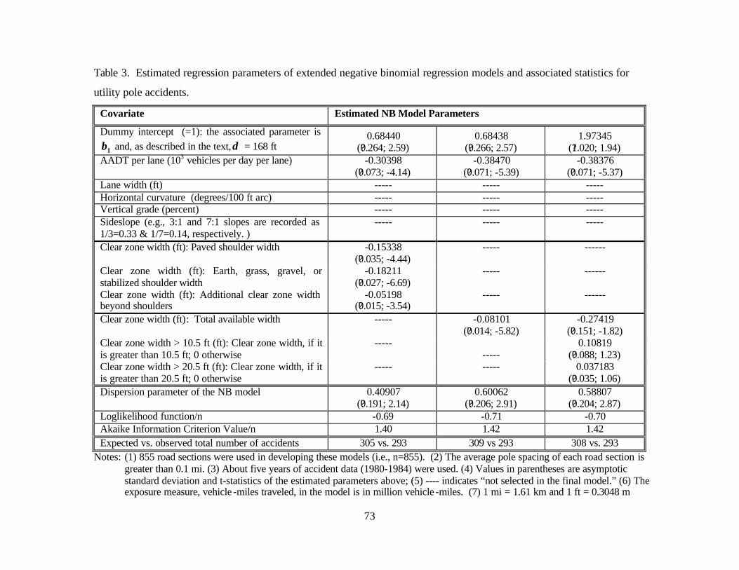
73
Table 3. Estimated regression parameters of extended negative binomial regression models and associated statistics for
utility pole accidents.
Covariate Estimated NB Model Parameters
Dummy intercept (=1): the associated parameter is β1 and, as described in the text,δ = 168 ft
0.68440 (?0.264; 2.59)
0.68438 (?0.266; 2.57)
1.97345 (?1.020; 1.94)
AADT per lane (103 vehicles per day per lane) -0.30398 (?0.073; -4.14)
-0.38470 (?0.071; -5.39)
-0.38376 (?0.071; -5.37)
Lane width (ft) ----- ----- ----- Horizontal curvature (degrees/100 ft arc) ----- ----- ----- Vertical grade (percent) ----- ----- ----- Sideslope (e.g., 3:1 and 7:1 slopes are recorded as 1/3=0.33 & 1/7=0.14, respectively. )
-----
-----
-----
Clear zone width (ft): Paved shoulder width -0.15338 (?0.035; -4.44)
-----
------
Clear zone width (ft): Earth, grass, gravel, or stabilized shoulder width
-0.18211 (?0.027; -6.69)
-----
------
Clear zone width (ft): Additional clear zone width beyond shoulders
-0.05198 (?0.015; -3.54)
-----
------
Clear zone width (ft): Total available width -----
-0.08101 (?0.014; -5.82)
-0.27419 (?0.151; -1.82)
Clear zone width > 10.5 ft (ft): Clear zone width, if it is greater than 10.5 ft; 0 otherwise
----- -----
0.10819 (?0.088; 1.23)
Clear zone width > 20.5 ft (ft): Clear zone width, if it is greater than 20.5 ft; 0 otherwise
-----
-----
0.037183 (?0.035; 1.06)
Dispersion parameter of the NB model 0.40907 (?0.191; 2.14)
0.60062 (?0.206; 2.91)
0.58807 (?0.204; 2.87)
Loglikelihood function/n -0.69 -0.71 -0.70 Akaike Information Criterion Value/n 1.40 1.42 1.42 Expected vs. observed total number of accidents 305 vs. 293 309 vs 293 308 vs. 293
Notes: (1) 855 road sections were used in developing these models (i.e., n=855). (2) The average pole spacing of each road section is greater than 0.1 mi. (3) About five years of accident data (1980-1984) were used. (4) Values in parentheses are asymptotic standard deviation and t-statistics of the estimated parameters above; (5) ---- indicates “not selected in the final model.” (6) The exposure measure, vehicle -miles traveled, in the model is in million vehicle -miles. (7) 1 mi = 1.61 km and 1 ft = 0.3048 m
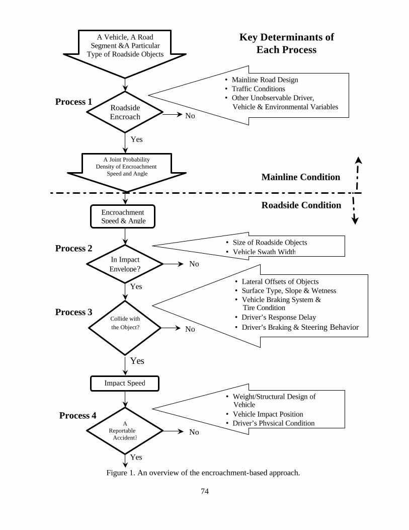
74
Figure 1. An overview of the encroachment-based approach.
A Vehicle, A Road Segment &A Particular
Type of Roadside Objects
Roadside Encroach No
Yes
• Mainline Road Design • Traffic Conditions • Other Unobservable Driver, Vehicle & Environmental Variables
Key Determinants of Each Process
Mainline Condition
Process 1
Roadside Condition
In Impact Envelope?
Encroachment Speed & Angle
Collide with the Object?
Impact Speed
Yes
Yes
No
No
• Size of Roadside Objects • Vehicle Swath Width
• Lateral Offsets of Objects • Surface Type, Slope & Wetness • Vehicle Braking System & Tire Condition • Driver’s Response Delay • Driver’s Braking & Steering Behavior
Process 2
Process 3
A Reportable
Accident?
Yes
No
• Weight/Structural Design of Vehicle • Vehicle Impact Position • Driver’s Physical Condition
Process 4
A Joint Probability Density of Encroachment
Speed and Angle
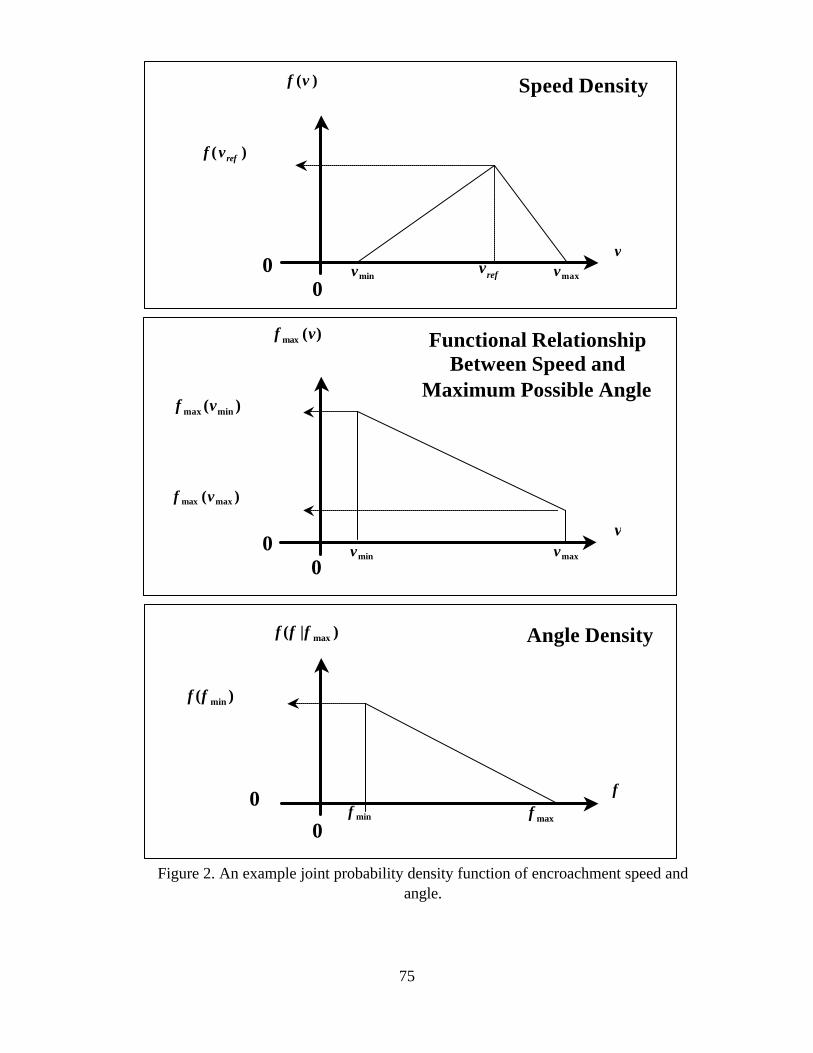
75
7
Figure 2. An example joint probability density function of encroachment speed and angle.
φmin φmax
0
0
φ
f ( )minφ
Angle Density f ( | )maxφ φ
0 v
vmaxvmin
Functional Relationship Between Speed and
Maximum Possible Angle
φmax ( )v
φmax min( )v
φmax max( )v
0
f v( )
0 v
f vref( )
vref vmaxvmin
Speed Density
0

76
Figure 3. Impact envelope of a roadside object for a given vehicle encroachment angle.
l lenv obj veh objW W= + +csc( ) cot( )φ φ
Roadside Object
Wveh
φl obj
WobjDobj
Wobj
Zone 1
Zone 2
Zone 3
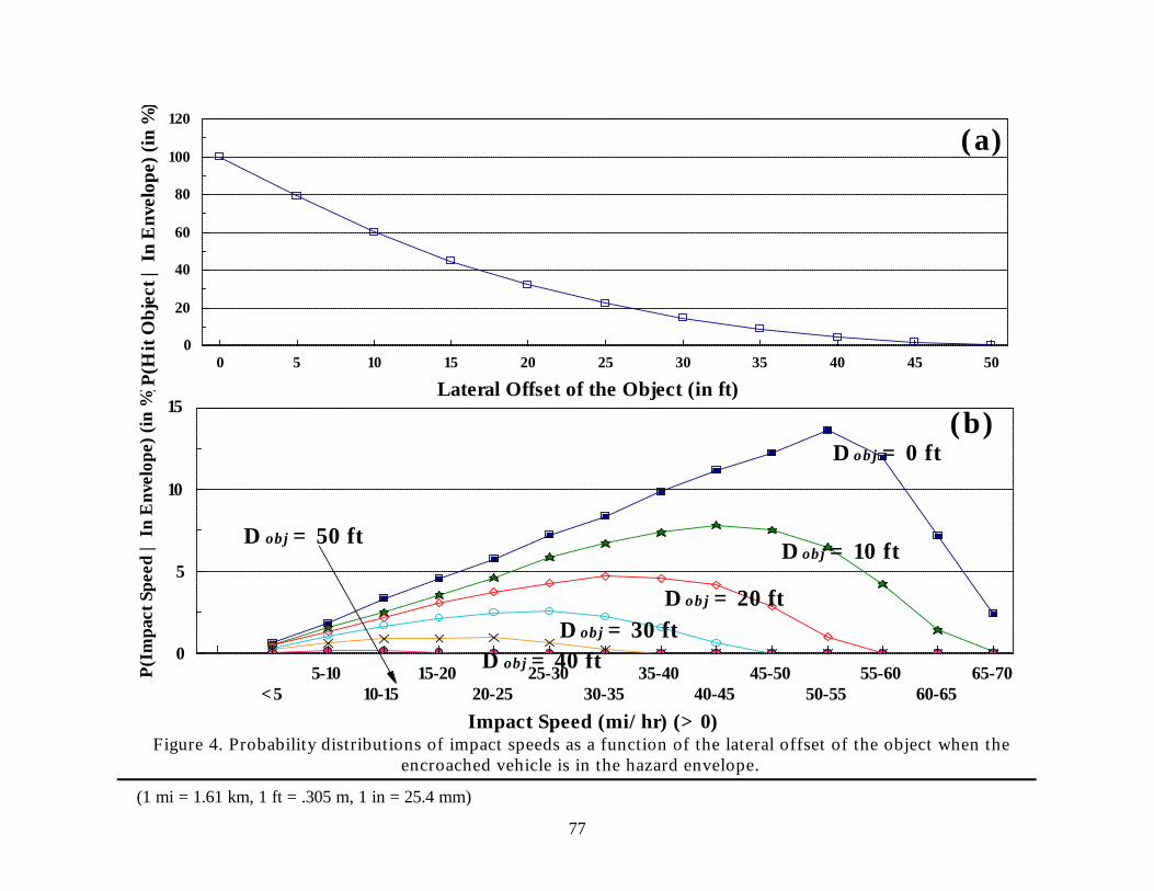
77
Figure 4. Probability distributions of impact speeds as a function of the lateral offset of the object when the encroached vehicle is in the hazard envelope.
<55-10
10-1515-20
20-2525-30
30-3535-40
40-4545-50
50-5555-60
60-6565-70
Impact Speed (mi/hr) (> 0)
0
5
10
15
P(Im
pact
Spe
ed |
In
Env
elop
e) (i
n %
)
D obj = 0 ft
D obj = 10 ft
D obj = 20 ftD obj = 30 ft
D obj = 40 ft
D obj = 50 ft
(b)
(a)
0 5 10 15 20 25 30 35 40 45 50
Lateral Offset of the Object (in ft)
0
20
40
60
80
100
120
P(H
it O
bjec
t | I
n E
nvel
ope)
(in
%)
(1 mi = 1.61 km, 1 ft = .305 m, 1 in = 25.4 mm)
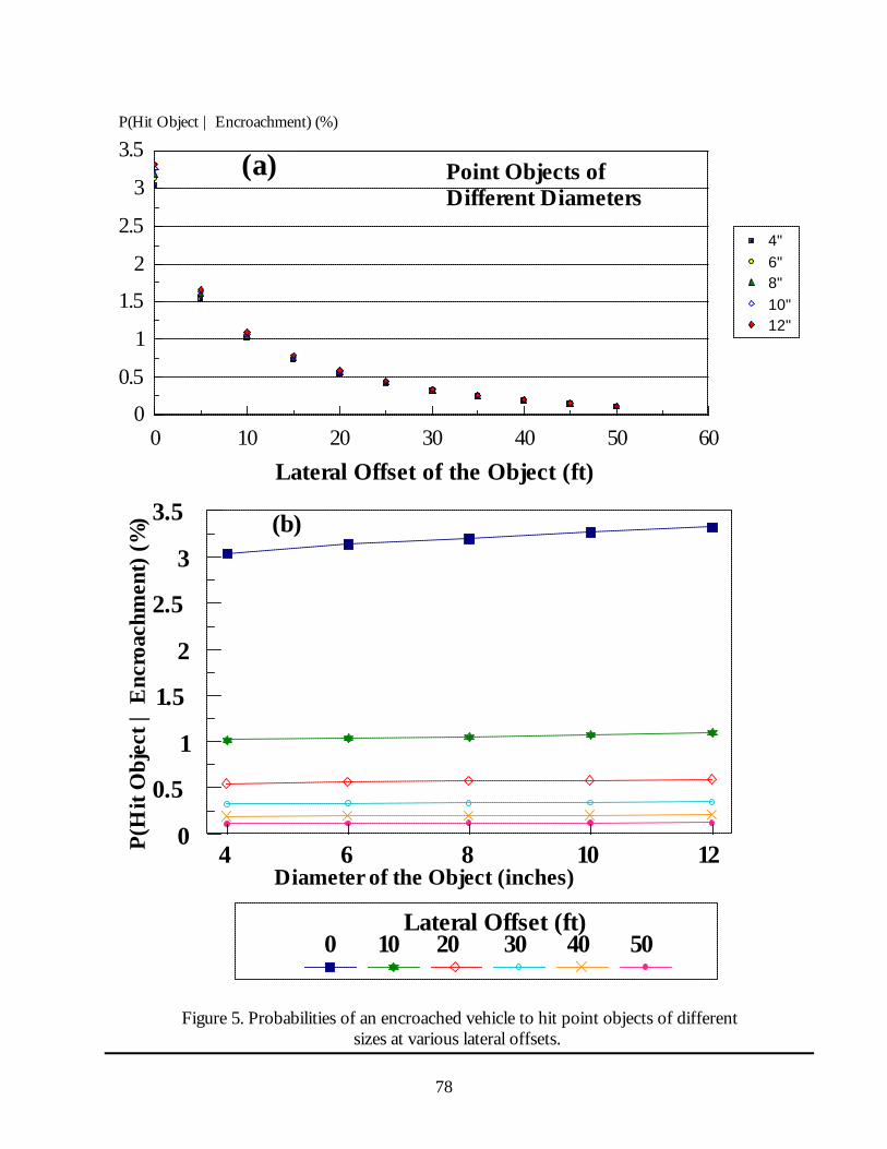
78
0 10 20 30 40 50 60
Lateral Offset of the Object (ft)
0
0.5
1
1.5
2
2.5
3
3.5P(Hit Object | Encroachment) (%)
4"6"8"10"12"
Point Objects of Different Diameters
(a)P(
Hit
Obj
ect |
Enc
roac
hmen
t) (%
)
4 6 8 10 120
0.5
1
1.5
2
2.5
3
3.5
Diameter of the Object (inches)
Lateral Offset (ft)0 20 30 40 5010
(b)
Figure 5. Probabilities of an encroached vehicle to hit point objects of different sizes at various lateral offsets.

79
Figure 6. Probabilities of an encroached vehicle to hit continuous objects of different lengths at various lateral offsets.
0 10 20 30 40 500
10
20
30
40
50
60
Lateral Offset of the Object (ft)
P(H
it O
bjec
t | E
ncro
achm
ent)
(%)
100'
250'
500'
750'
1000'
1500'
2000'
2500'
Continuous Objects of Different Lengths (per side of the road)
(a)
0 500 1,000 1,500 2,000 2,5000
10
20
30
40
50
60
Length of the Object (ft)
P(H
it O
bjec
t | E
ncro
achm
ent)
(%) 0'
5'
10'
15'
20'
25'
30'
35'
40'
45'
50'
Different Lateral Offsets
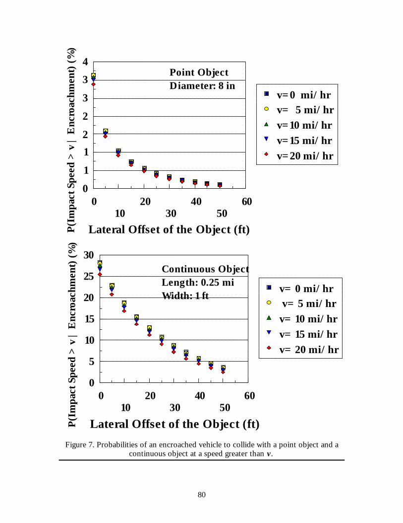
80
Point ObjectDiameter: 8 in
Continuous ObjectLength: 0.25 miWidth: 1 ft
Figure 7. Probabilities of an encroached vehicle to collide with a point object and a continuous object at a speed greater than v.
010
2030
4050
60
Lateral Offset of the Object (ft)
0
5
10
15
20
25
30
P(Im
pact
Spe
ed >
v |
Enc
roac
hmen
t) (%
)
v= 0 mi/hr v= 5 mi/hrv= 10 mi/hrv= 15 mi/hrv= 20 mi/hr
010
2030
4050
60
Lateral Offset of the Object (ft)
0
1
1
2
2
3
3
4P(
Impa
ct S
peed
> v
| E
ncro
achm
ent)
(%)
v=0 mi/hrv= 5 mi/hrv=10 mi/hrv=15 mi/hrv=20 mi/hr
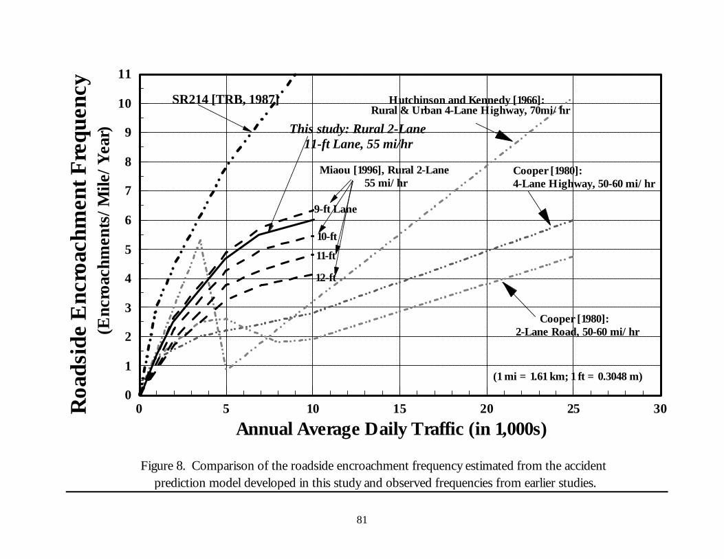
81
0 5 10 15 20 25 300
1
2
3
4
5
6
7
8
9
10
11
Annual Average Daily Traffic (in 1,000s)
Hutchinson and Kennedy [1966]: Rural & Urban 4-Lane Highway, 70mi/hr
Cooper [1980]: 4-Lane Highway, 50-60 mi/hr
Cooper [1980]: 2-Lane Road, 50-60 mi/hr
9-ft Lane
10-ft
11-ft
12-ft
This study: Rural 2-Lane 11-ft Lane, 55 mi/hr
Miaou [1996], Rural 2-Lane 55 mi/hr
Figure 8. Comparison of the roadside encroachment frequency estimated from the accidentprediction model developed in this study and observed frequencies from earlier studies.
Roa
dsid
e E
ncro
achm
ent F
requ
ency
(Enc
roac
hmen
ts/M
ile/Y
ear)
(1 mi = 1.61 km; 1 ft = 0.3048 m)
SR214 [TRB, 1987]

82
0 2 4 6 8 10 12Annual Average Daily Traffic (1000s)
0
5
10
15
20
25R
oads
ide
Enc
roac
hmen
ts (p
er m
ile p
er y
ear)
Delta=168 ft, Model 3Delta=168 ft, Model 1Delta=69.4 ft, Model 3Delta=69.4 ft, Model 1Delta=34.3 ft, Model 3Delta=34.3 ft, Model 1
Figure 9. Roadside encroachment frequencies estimated from two utility pole accident models under three different sizes of hazard envelopes.
(1 mi = 1.61 km, 1 ft = .305 m, 1 in = 25.4 mm)
83
APPENDIX C
RESEARCH STATEMENT ESTIMATING ROADSIDE ENCROACHMENT RATES WITH THE
COMBINED STRENGTHS OF ACCIDENT- AND ENCROACHMENT-BASED APPROACHES
Prepared by
Shaw-Pin Miaou, Ph.D. Center for Transportation Analysis
Oak Ridge National Laboratory October 24, 1997
BACKGROUND
Models used in previous studies to quantify the relationships between run-off-the-road (ROR)
accidents and roadside hazards, such as utility poles, trees, guardrail, median barriers, and
embankments, have been categorized as using either an accident-based approach or an
encroachment-based approach. The former, which uses the Poisson and negative binomial (NB)
types of regression models, has a solid statistical ground, but has been criticized as being overly
empirical and lacking engineering basis. The latter, on the other hand, has analytical and
engineering strengths, but has been described as being full of subjective assumptions and lacking
sufficient supporting data. Historically, researchers on roadside safety seem to have treated the
accident-based and encroachment-based approaches as two competing, disconnected approaches
and seldom or never attempt to seek the opportunity to combine the strengths of both.
In the last 15 years or so, despite its limitations, encroachment-based cost-effectiveness
procedures have gained increasing application in determining the need for roadside safety
improvements and for developing general selection guidelines for roadside safety hardware.
Some procedures have been adopted as part of the AASHTO’s roadside design guideline
[AASHTO, 1989]. More importantly, the approach will form the basis of the roadside model in
the Accident Analysis Module (AAM) of the Interactive Highway Safety Design Model
(IHSDM) that is currently being developed by the Federal Highway Administration (FHWA)
[Griffith and Bared, 1997].
Vehicle roadside encroachment characteristics, including the encroachment rate or encroachment
probability, are key input parameters to the encroachment-based cost-effectiveness procedures.

84
The reliability of the results from the procedures is directly affected by the quality of these input
parameters. At present, it appears that available encroachment data to estimate these input
parameters are extremely limited and largely outdated--some were collected over 30 years ago
on a small number of road sections. The FHWA and Transportation Research Board (TRB) have
been addressing the requirements and collection of such data through their sponsorship of several
roadside safety projects. As a result, rather comprehensive data collection plans have been
proposed, and results of pilot data collection efforts have been reported [Mak and Sicking, 1992;
Daily et al., 1997; Mak and Bligh, 1996]. A review of these plans and pilot data collection results
suggests that the cost of collecting the required roadside field data will be very high.
Furthermore, the validity of any field-collected encroachment data may be questionable because
of the technical difficulty in distinguishing between controlled (or intentional) and uncontrolled
(or unintentional) encroachments.
In two recent studies by Miaou [1996 and August, 1997], he proposed a method to estimate
roadside encroachment rates using accident-based models. The method combines the strengths
of both the accident-based and encroachment-based approaches. Specifically, it incorporates the
analytical and engineering strengths of the encroachment-based models into the formulation of
the mean function of accident-based models. Note that the mean function in accident-based
regression models specifies the functional relationship between the expected accident rate and
covariates (or independent variables). Miaou further illustrated the use of such a method to
estimate roadside encroachment rates for rural two- lane, undivided roads using data from the
FHWA Seven States Cross-Section Data Base [Rodgman et al., 1989].
Three illustrations have been conducted in Miaou’s studies. In the first illustration, all ROR
accidents were considered. Among other mainline design and traffic variables, general roadside
hazard indices which include sampling distributions of clear zone width and sideslope along each
road section were used in developing ROR accident-based prediction models. In the second and
third illustrations, accidents involving a specific type of roadside hazards were considered.
Specifically, guardrail and utility pole accidents were considered in the second and third
illustrations, respectively. The lateral offset of individual roadside hazards was the main
roadside design variable considered in developing models. The estimated roadside encroachment

85
rates were found to be consistent among the three illustrations and compatible with those
estimated by earlier encroachment-based studies in terms of their order of magnitude. These
results indicate that the proposed method can be a viable approach to estimating encroachment
rates without actually collecting the encroachment data that can be expensive and technically
difficult.
At the conceptual and analytical levels, the strengths of the proposed method can be summarized
as follows:
(1) It is straightforward to estimate encroachment rates for various mainline design and traffic
conditions, e.g., for different lane width, horizontal curvature, vertical grade, and traffic
volumes, provided that adequate mainline data are available to develop the accident-based
model. To actually collect such detailed encroachment data will be very expensive and may
not even be practical.
(2) When good roadside accident history is available for individual sites, site-specific
encroachment rates can potentially be obtained with the proposed method by using the
Empirical Bayes (EB) method. This allows site-specific driver, vehicle, and environmental
factors that are not available in developing accident-based models to be reflected in an
objective way in the final encroachment rate estimate. (Note that this cannot be done in any
objective way with the current encroachment-based methods.) Since the roadway model in
the AAM of IHSDM will use EB estimator when accident history is available for individual
sites [Griffith and Bared, 1997], this strength of the proposed method enables the roadway
and roadside models to adopt the same statistical estimation procedure and, therefore, it will
increase the probability of obtaining consistent estimates from the two models within the
AAM.
(3) Provided a flexible mean functional form is used in developing accident-based models, the
encroachment rates estimated from the proposed method are relatively unaffected by the
underreporting of minor accidents. This strength has been explained in two different ways in
the two studies by Miaou [1996 and August 1997], one of which used encroachment-based
approach to illustrate this point.
(4) The estimated encroachment rate is based on ROR accident data and is, therefore,

86
uncontaminated by controlled encroachments. Unlike field-collected encroachment data,
there is no need to develop a procedure to distinguish between controlled and uncontrolled
encroachments (which can be subjective and technically challenging).
(5) Standard statistical inferences, especially the sampling error (or sampling variability), can be
readily provided for the estimated encroachment rates. (Note, however, that the generation
of these inferences can be computationally intensive.)
(6) Because accident, traffic, and roadway data, such as those contained in the Highway Safety
Information System (HSIS), are constantly being collected, updated, and maintained. The
estimated encroachment rates can be updated frequently, if necessary, using the latest data
with a marginal cost.
(7) In the proposed method, the formulation of the mean function in developing the accident-
based model (an NB regression-based model) takes into account the analytical procedure
used in the encroachment-based model which is guided by driver behavior, vehicle dynamics,
and traffic flow theories. This approach to formulation, again, increases the chance of
obtaining consistent estimates of roadway and roadside accident rates from the roadway and
roadside models in the AAM of the IHSDM.
Despite these conceptual and analytical strengths, the consistency of the proposed method has
only been illustrated using the data from one data base. In addition, the accident data contained
in the data base are not up-to-date (from 1980 to 1984). It is important that the consistency of
the proposed method be “validated” with independent and more up-to-date data sets. A research
plan to “validate” the proposed method is described in the following section.
PROPOSED RESEARCH PLAN
We propose that the consistency of Miaou’s method be “validated” with Minnesota and
Washington data from the HSIS. Specifically, the data sets to be employed are those used by
Bared and Vogt [1997] in developing rural two- lane roadway models for the AAM. They have
developed promising NB regression models for total road segment accidents using these two data
sets. Their models are considered quite complete in terms of the number and type of geometric
design variables that are included in the model and are up-to-date in terms of the accident data
considered. Because roadside data are generally not available in State road inventory data base,

87
most of the roadway models developed by previous studies did not consider roadside variables.
An important feature of Bared and Vogt’s model is that it includes a general roadside hazard
index, called roadside hazard rating, which were collected from a video- log system maintained at
FHWA. Because Bared and Vogt’s models are quite promising, they are likely to be adopted as
the “base roadway model” in the AAM for a typical (or ideal) design and for establishing
accident modification factors for alternative designs.
In the light of these developments in roadway models, there are several advantages of
“validating” Miaou’s method with these two data sets:
(1) The roadside hazard rating, as collected by Bared and Vogt, can be readily used in
“validating” the method without new roadside data collection effort.
(2) The data have been quality checked by Bared and Vogt, which will increase the chance of
developing good encroachment rate estimates and will reduce data preparation cost.
(3) If Bared and Vogt’s models are adopted as part of the roadway model of AAM, then using
the same data sets (as those used by Bared and Vogt) to develop the encroachment rates for
roadside models will increase the probability of obtaining consistent roadway and roadside
estimates from the two models.
PROPOSED TASKS
The specific tasks to be conducted under this plan include:
Task A: Obtain and review MN and WA data.
Task B: Prepare the data in a suitable format for developing accident prediction models.
Task C: Develop accident prediction models using MN and WA data.
Because accident types are organized differently in Washington and Minnesota, it may not be
meaningful to develop one combined model for run-off-the-road accidents for the two States.
In this task, we will try to build models for each State and study the feasibility of developing
a combined model for the two States. The extended NB regression model developed by
Miaou will be used in this study.
Task D: Estimate roadside encroachment rates.
88
If reasonable accident prediction models are developed in Task C, roadside encroachment
rates will be generated using the accident prediction model proposed by Miaou [1996 and
August 1997]. And, if feasible, these rates will be generated by AADT, lane width,
horizontal curvature, and vertical grade.
Task E: Develop encroachment adjustment factors for horizontal curvature and vertical grade.
Task F: Prepare a draft report to summarize the study.
Task G: Prepare a final report.
REFERENCES
1. American Association of State Highway and Transportation Officials (AASHTO) (1989) Roadside Design Guide. Washington, D.C.
2. Bared, J.G. and Vogt, A. (1997) Accident Models for Two-Lane Rural Highways. Paper submitted to Transportation Research Board (TRB) for presentation in the 77th TRB Annual Meeting and for publication in Transportation Research Record.
3. Daily, K., Hughes, W., and McGee, H. (1997) Experimental Plans for Accident Studies of Highway Design Elements: Encroachment Accident Study. FHWA-RD-96-081. FHWA, U.S. Department of Transportation.
4. Griffith, M.S., and Bared, J.G. Overview of the Accident Analysis Module of the Interactive Highway Safety Design Model. Unpublished paper. Federal Highway Administration, June 3, 1997.
5. Mak, K.K., and Sicking, D.L. (1992) Development of Roadside Safety Data Collection Plan. Technical Report, Texas Transportation Institute, Texas A&M University System, College Station, Texas.
6. Mak, K.K., and Bligh, R.P. (1996) Recovery-Area Distance Relationships for Highway Roadsides. Phase I Report, NCHRP Project G17-11.
7. Miaou, S.-P. (1996) Measuring the Goodness-of-Fit of Accident Prediction Models. FHWA-RD-96-040. FHWA, U.S. Department of Transportation.
8. Miaou, S.-P. Another Look at the Relationship Between Accident- and Encroachment-Based Approaches to Run-Off-the-Road Accidents Modeling. Working Paper. Center for Transportation Analysis, Oak Ridge National Laboratory, Oak Ridge, Tennessee, August 1997.
9. Rodgman, E., Zegeer, C., and Hummer, J. (1989) Safety Effects of Cross-Section Design for Two-Lane Roads - Data Base User's Guide. Report submitted to FHWA, Revised, November.