estimating profile soil moisture and groundwater variations using grace...

Estimating profile soil moisture and groundwater variations

using GRACE and Oklahoma Mesonet soil moisture data

Sean Swenson,1 James Famiglietti,2 Jeffrey Basara,3 and John Wahr4

Received 22 March 2007; revised 3 August 2007; accepted 5 October 2007; published 10 January 2008.

[1] In this study we estimate a time series of regional groundwater anomalies bycombining terrestrial water storage estimates from the Gravity Recovery and ClimateExperiment (GRACE) satellite mission with in situ soil moisture observations from theOklahoma Mesonet. Using supplementary data from the Department of Energy’sAtmospheric Radiation Measurement (DOE ARM) network, we develop an empiricalscaling factor with which to relate the soil moisture variability in the top 75 cm sampledby the Mesonet sites to the total variability in the upper 4 m of the unsaturated zone. Bysubtracting this estimate of the full unsaturated zone soil moisture anomalies, we arrive ata time series of groundwater anomalies, spatially averaged over a region approximately280,000 km2 in area. Results are compared to observed well level data from a largersurrounding region, and show consistent phase and relative inter-annual variability.

Citation: Swenson, S., J. Famiglietti, J. Basara, and J. Wahr (2008), Estimating profile soil moisture and groundwater variations

using GRACE and Oklahoma Mesonet soil moisture data, Water Resour. Res., 44, W01413, doi:10.1029/2007WR006057.

1. Introduction

[2] Water stored below the Earth’s surface is fundamen-tally important to the well-being of most of the world’sinhabitants. Nearly half the population of the U.S. usegroundwater as their primary source of drinking water[Bartolino and Cunningham, 2003], and approximately40% of irrigation water is extracted from the ground.Furthermore, ‘‘No comprehensive national groundwater-level network exists with uniform coverage of major aqui-fers, climate zones, and land uses’ [Hutson et al., 2004].Globally, the situation is the same or worse, with manyregions experiencing depletion, salinization, or contamina-tion of their groundwater supply [Shah et al., 2000].Groundwater stores are experiencing increasing demands,and proper management of these resources requires bettermonitoring and assessment.[3] Remotely sensed data have been used extensively to

monitor surface and near-surface components of the watercycle, e.g., altimetric measurements of river and lake height[Alsdorf and Lettenmaier, 2003], microwave estimation ofsoil moisture [Njoku et al., 2003] and snow water equivalent[Kelly et al., 2004]. Characterizing the stores and fluxes ofsub-surface water has proven less tractable to typicalsatellite methods. Because groundwater is stored belowthe land surface, nearly all methods must rely on indirectmeasures of various aspects of groundwater hydrology.

These include remote sensing of surface fractures andlineaments, vegetation along springs, surface displacementsdue to aquifer inflation and compaction, surface waterbodies, and localized recharge features [Becker, 2006].One exception is the use of data from the Gravity Recoveryand Climate Experiment (GRACE), which is sensitive tochanges in the total water column [Wahr et al., 1998;Swenson et al., 2006]. Yeh et al. [2006] demonstrated thatregional average variations in groundwater could be reli-ably estimated by combining GRACE estimates of verti-cally integrated water storage with independent estimatesof unsaturated zone storage using a water balance ap-proach. (We use the term groundwater to refer to thesaturated zone only, while the terms soil moisture contentand unsaturated zone water content will be used somewhatinterchangably.)[4] In this paper, we apply the water balance approach

used by Yeh et al. [2006] to estimate variations in ground-water averaged over a region centered on the state ofOklahoma in the Central U.S. As for the region studied inthat paper (Illinois), the primary contributors to changes inthe Oklahoma regional water balance are soil moisture andgroundwater; snow and surface water are assumed negligi-ble [Rodell and Famiglietti, 2001]. To estimate regionalaverage soil moisture, we utilize observations from theOklahoma Mesonet [Brock et al., 1995]. The OklahomaMesonet (OM) is an automated observing network, collect-ing real-time hydrometeorological observations from morethan a hundred stations throughout Oklahoma. As part ofthe suite of observations made at many of these sites, soilmoisture measurements are made every 30 min at depthsof 5, 25, 60, and 75 cm using Campbell Scientific 229-Lheat dissipation sensors [Basara and Crawford, 2000]. Bycombining these data with total column water storageestimates from GRACE in a water balance equation, wecompute a time series of spatially averaged groundwaterstorage variations.

1Advanced Study Program, National Center for Atmospheric Research,Boulder, Colorado, USA.

2Department of Earth System Science, University of California, Irvine,California, USA.

3Oklahoma Climatological Survey, University of Oklahoma, Norman,Oklahoma, USA.

4Department of Physics and CIRES, University of Colorado, Boulder,Colorado, USA.

Copyright 2008 by the American Geophysical Union.0043-1397/08/2007WR006057

W01413

WATER RESOURCES RESEARCH, VOL. 44, W01413, doi:10.1029/2007WR006057, 2008

1 of 12

[5] The study of Yeh et al. [2006] was made possible bythe existence of an extensive monitoring network of bothsoil moisture and groundwater well levels operated by theIllinois State Water Survey (ISWS) [Hollinger and Isard,1994]. This network is perhaps unique by virtue of itscombination of areal extent (�200,000 km2), a long andup-to-date period of record, and measurement of all signif-icant water balance components. While the OklahomaMesonet shares the first two characteristics with the ISWSnetwork, the third is unfortunately a point of departure.[6] Tens of thousands of wells exist in Oklahoma, but

only a few are monitored more frequently than once peryear. Moreover, the parameters (e.g., specific yield) neces-sary to convert well level to water storage are difficult toobtain and uncertain. Thus the ability to assess a remotelysensed groundwater estimate with in situ observations islimited, and this should be kept in mind when interpretingthe comparison between a GRACE-derived groundwaterestimate to an in situ estimate shown later in the paper.[7] Another concern regarding the OM soil moisture data

are their representativeness. Because the water table isrelatively shallow in Illinois, the ISWS soil moisture mea-surements (which span the upper 2 m) effectively representthe entire unsaturated zone, and therefore the separation ofthe GRACE total column water storage is relatively straight-forward in this case. In Oklahoma, however, where themean water table depth is usually tens of meters deep, thereare significant variations in unsaturated zone water storagebelow 75 cm depth (the deepest OM sensor depth) that arenot captured by the OM soil moisture sensors. We addressthis issue here by utilizing an empirical method for esti-mating deeper soil moisture from near-surface observations,before creating a more robust residual groundwater esti-mate. Because the groundwater estimate is the residual termin a water balance equation, failure to sample the total

unsaturated soil moisture signal will lead to greater errors inour groundwater estimate. The method we describe toaccount for deeper soil moisture is applied here to theregion of the Southern Great Plains of the U.S., but isapplicable to other observational data sets, whether in situ orremotely sensed, that may not fully sample the variabilitypresent in the unsaturated zone.

2. Data

2.1. GRACE

[8] The GRACE satellite mission, jointly sponsored byNASA and its German counterpart DLR, has been collect-ing data since mid-2002. The nominal product of themission is a series of monthly Earth gravity fields [Tapleyet al., 2004]. However, by exploiting the direct relationshipbetween changes in the gravity field and changes in mass atthe Earth’s surface, the month-to-month gravity variationsobtained from GRACE can be used to make global esti-mates of vertically integrated terrestrial water storage with aspatial resolution of a few hundred km and greater, withhigher accuracy at larger spatial scales [Wahr et al., 2004;Swenson et al., 2003].[9] GRACE data have been used in a number of studies

to estimate water storage variability, e.g., to estimate terres-trial water storage variations from the scale of large riverbasins [Crowley et al., 2006; Seo et al., 2006] to thecontinents [Schmidt et al., 2006; Tapley et al., 2004], forestimating groundwater storage variations [Rodell et al.,2006; Yeh et al., 2006], for ice sheet and glacier mass lossstudies [Velicogna and Wahr, 2006; Tamisiea et al., 2005]and for estimating hydrologic fluxes including evapotrans-piration [Rodell et al., 2004], precipitation minus evapo-transpiration [Swenson and Wahr, 2006b], and discharge[Syed et al., 2005].

Figure 1. Map of Central U.S. showing locations of OM soil moisture sites. Contours indicate values ofGRACE averaging kernel.

2 of 12

W01413 SWENSON ET AL.: GRACE ESTIMATES OF GROUNDWATER VARIABILITY IN OKLAHOMA W01413

[10] In this study, we use Release 4 (RL04) data producedby the Center for Space Research (CSR) which incorporatenumerous improvements in the gravity field determinationprocess. Additionally, we apply the post-processing tech-nique of Swenson and Wahr [2006a], which has been shownto produce water storage estimates that compare well within situ observations averaged over a region of 280,000 km2

surrounding Illinois [Swenson et al., 2006].

2.2. Soil Moisture Observations

2.2.1. Oklahoma Mesonet[11] The Oklahoma Mesonetwork (Mesonet) began in

1991 as a state-wide mesoscale environmental monitoringnetwork [Brock et al. 1995; McPherson et al., 2007]. Soilmoisture sensors were added to 60 sites and installed at fourdepths (5, 25, 60, and 75 cm) in 1996 and to 43 sites at twodepths (5 and 25 cm) in 1999 [Illston et al., 2007]. Data arecollected every 30 min and processed at the OklahomaClimatological Survey (OCS) at the University of Okla-homa. A series of automated and manual processes maintainquality control and convert the raw data into daily averagevalues of volumetric soil water content [Illston et al., 2007].Figure 1 shows the Oklahoma Mesonet (OM) locations usedin this study, as well as the contours of the averaging kernelused to compute the GRACE water storage time series.[12] The soil moisture sensor deployed at OM sites is the

Campbell Scientific 229-L heat dissipation sensor. Thissensor measures its change in temperature after a heat pulsehas been introduced [Basara and Crawford, 2000; Illston etal., 2007]. During installation of the soil moisture sensors,soil cores from each site and each depth are analyzed for thesoil characteristics. Using the measured temperature differ-ence of the sensor before and after heating (i.e., heatdissipation) and the soil characteristics, hydrological varia-bles such as soil water content and soil matric potential canbe calculated.[13] The volumetric water content is determined from a

soil water retention curve. Using detailed soil characteristics

and soil bulk density measurements collected at each sensorlocation, soil water retention curves were estimated usingthe Arya and Paris [1981] methodology. A number ofautomated algorithms assess the quality of the soil moisturedata. In general, the algorithms ensure that the data arereporting within operational ranges, the calibration coeffi-cients are correct, and the soil is not frozen.2.2.2. DOE ARM Network[14] Significant soil water variability occurs below the

deepest OM sensor depth of 75 cm. To accurately estimate aresidual groundwater signal, the full contribution from theunsaturated zone must be removed from the total columnsignal as determined from GRACE data; any inaccuracies inthe removed signal will contaminate the groundwater esti-mate. Observations of deeper soil moisture in this regioncan be obtained, although with less dense spatial coverage,from the Department of Energy’s Southern Great PlainsAtmospheric Radiation Measurement (DOE ARM) network[Schneider et al., 2003].[15] The DOE ARM network has 21 automated soil water

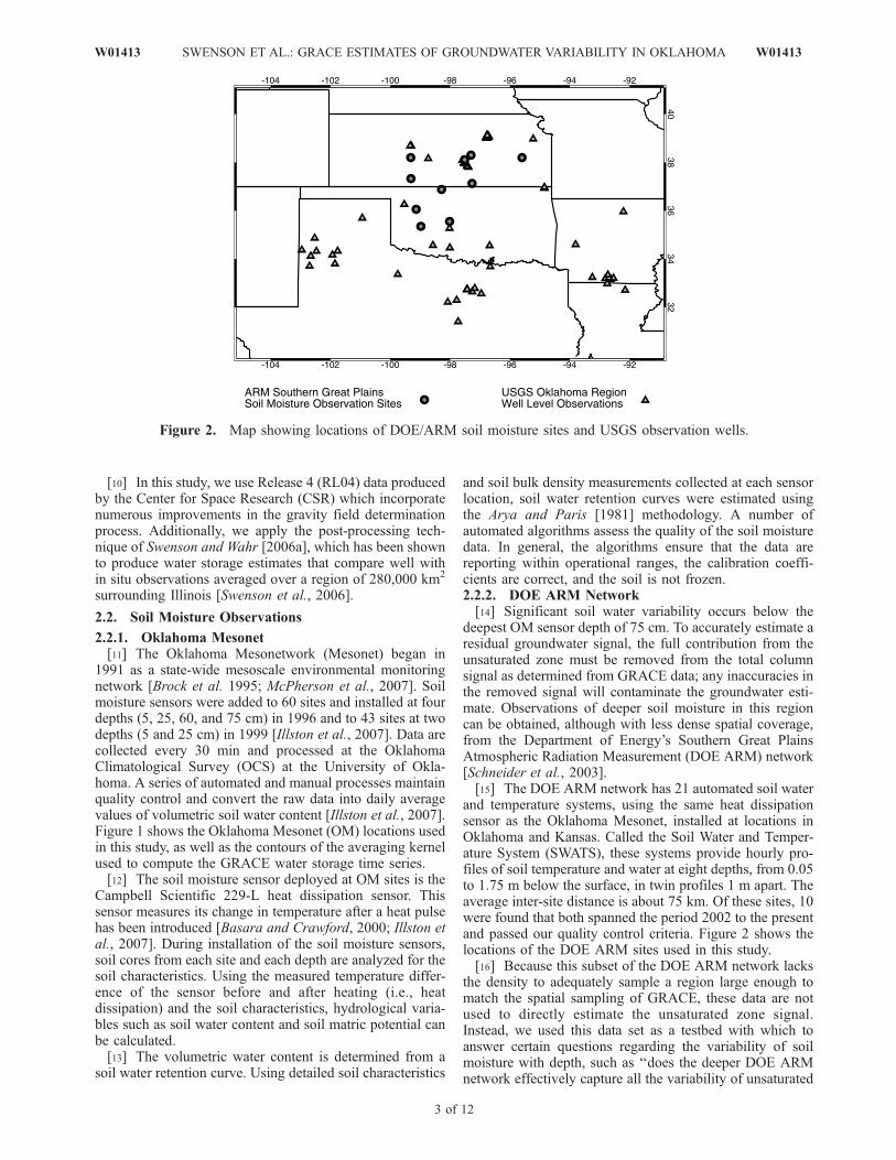
and temperature systems, using the same heat dissipationsensor as the Oklahoma Mesonet, installed at locations inOklahoma and Kansas. Called the Soil Water and Temper-ature System (SWATS), these systems provide hourly pro-files of soil temperature and water at eight depths, from 0.05to 1.75 m below the surface, in twin profiles 1 m apart. Theaverage inter-site distance is about 75 km. Of these sites, 10were found that both spanned the period 2002 to the presentand passed our quality control criteria. Figure 2 shows thelocations of the DOE ARM sites used in this study.[16] Because this subset of the DOE ARM network lacks

the density to adequately sample a region large enough tomatch the spatial sampling of GRACE, these data are notused to directly estimate the unsaturated zone signal.Instead, we used this data set as a testbed with which toanswer certain questions regarding the variability of soilmoisture with depth, such as ‘‘does the deeper DOE ARMnetwork effectively capture all the variability of unsaturated

Figure 2. Map showing locations of DOE/ARM soil moisture sites and USGS observation wells.

W01413 SWENSON ET AL.: GRACE ESTIMATES OF GROUNDWATER VARIABILITY IN OKLAHOMA

3 of 12

W01413

zone soil moisture?’’, ‘‘if not, can one develop a model toextrapolate these data to depth?’’, and ‘‘does such a modelreveal a robust relationship between variability in near-surface soil moisture and that of the entire unsaturatedzone?’’. The result of this analysis, described below, is ascaling relationship between variability in the upper 75 cmto that of the entire unsaturated zone, thus allowing theestimation of a full unsaturated zone signal from the OMdata.

3. Methods

3.1. GRACE

[17] Each monthly GRACE gravity field is composed of aset of spherical harmonic (Stokes) coefficients. Degree 1terms are not part of the solution, so they are estimated froma combined land-surface/ocean model. After removal of thetemporal mean and conversion of the gravity field anoma-lies to an equivalent water thickness, each monthly field issubjected to a two-stage filtering process by applying firstthe Swenson and Wahr [2006a] decorrelation filter, followedby a Gaussian filter with a half-width corresponding to300 km [Wahr et al., 1998]. Spatial averaging of GRACEdata, via the Gaussian filter, is necessary to reduce thecontribution of noisy short wavelength components of thegravity field solutions.[18] Additionally, the effects of postglacial rebound

(PGR) are also modeled and removed from the GRACEtime series. PGR is the ongoing, viscoelastic response of thesolid Earth to the deglaciation that occurred at the end ofthe last ice age. We modeled the PGR contributions to theStokes coefficients using the ICE-5G ice deglaciation modelof Peltier [2004], and convolving with visco-elastic Green’sfunctions based on Peltier’s [1996] VM2 viscosity model.[19] To assess the uncertainty in the filtered GRACE

coefficients, the method of Wahr et al. [2006] is used. Inbrief, the temporal RMS of the high-pass filtered portion of

each coefficient is used as an estimate of the upper boundon the random component of the error. This estimate isconservative, because intraannual variations in the signalwill be interpreted as error. The 1-sigma error estimates inthe spatially averaged GRACE time series are then calcu-lated from the estimates of uncertainty in the individualStokes coefficients [Swenson and Wahr, 2002].[20] To reduce the influence of errors in the monthly

GRACE estimates, we construct a smoothed seasonal timeseries by applying a low-pass filter to the original data. Thelow-pass filter consists of fitting six terms (annual sine andcosine, semi-annual sine and cosine, mean, and trend) to thetime series. These terms vary for different epochs due to thepresence of a moving set of weights, which take the form ofa Gaussian function centered on each epoch successively.The application of the low-pass filter reduces the impact ofmonthly errors and results in a smoothly varying timeseries, yet retains important interannual variability thatwould not be captured by examining the mean seasonalcycle for the time period spanned by the data.

3.2. Oklahoma Mesonet Data

[21] To derive a residual groundwater change estimate, aspatially averaged soil moisture estimate must be removedfrom the GRACE regional average time series. First, how-ever, we need to determine whether the Oklahoma Mesonetsoil moisture data capture the variability of the entireunsaturated zone.[22] Figure 3 shows the time series of soil moisture,

expressed as monthly anomalies (relative to the mean valueduring the period 2003–2006) of volumetric water contentat each of the four depths at which OM sensors are located,averaged over all sites. A phase lag with depth can be seen,consistent with the findings of other studies [e.g.,Hirabayashiet al., 2003; Wu et al., 2002; Entin et al., 2000]. Theamplitudes of the four layers, however, are quite similar,showing little dampening at 75 cm depth, implying signifi-

Figure 3. Regional average time series of monthly soil moisture anomalies sampled at four depths bythe OM network. X axis is time, in years, and y axis is volumetric water content.

4 of 12


cant variability in deeper layers. This finding motivates ouranalysis of the DOE ARM data, which extends another meterto 1.75 m depth. In the following section, we examine theDOE ARM data to determine the nature of the relationshipbetween soil moisture variability and depth in this region.

3.3. DOE ARM Data

[23] The availability of the DOE ARM data allows us toexplore the depth dependence of soil moisture below the75 cm lower limit of the OM network. As with the OM data,the hourly DOE ARM soil moisture observations at each of

Figure 4. Regional average time series of monthly soil moisture anomalies sampled at eight depths bythe DOE/ARM network. X axis is time, in years, and y axis is volumetric water content.

Figure 5. Spectral coefficients describing DOE/ARM soil moisture observations, plotted as a functionof depth. Each line represents the coefficients of an individual monthly epoch. Upper left: temporal mean;upper right: trend; lower left: annual amplitude; lower right: annual phase. Y-axes are depth belowsurface, in meters.


5 of 12

W01413

the two profiles at the ten sites are first combined to formmonthly averaged time series for each of the eight layers.[24] Figure 4 shows the monthly averaged soil moisture

anomalies, expressed as volumetric water content, for eachlayer as a function of time. The increasing phase lag withdepth seen in Figure 3 is also apparent in Figure 4.Additionally, for depths below about 20 cm, the amplitudeof the signal decreases with depth, although it is still a largefraction of the amplitude in the upper layers. This impliesthat even below 1.75 m depth, soil moisture variability issignificant. However, because the variation with depth ismore apparent in the deeper DOE ARM data set, it may bepossible to create a simple model with which to extrapolatethese observations to depth, and so better represent the fullunsaturated zone signal.[25] To provide a clearer picture of the depth dependence

of the soil moisture observations, we use a weightedspectral filter to estimate a four-term annual cycle (ampli-tude, phase, mean, and linear trend) at each monthly epoch.Two key aspects of the observed soil moisture variability asa function of depth are the amplitude damping and the phaselag. The spectral decomposition allows the effects of de-creasing amplitude and increasing phase lag with depth tobe considered independently [Wu et al., 2002]. The weightstake the form of a Gaussian taper with a halfwidth of threemonths. When the taper is centered on a particular month,the spectral filter is most sensitive to the nearest monthlyepochs. The coefficients describing the annual cycle thusvary with time, and retain the inter-annual variability thatwould be lost by examining only the mean annual cycle.[26] Figure 5 shows the spectral coefficients computed

from the monthly averaged soil moisture values, plotted as a

function of depth. Each line represents the coefficients ofeach layer for a particular month. The y axis spans 4 mdepth because it appears that the annual amplitude decays toa negligible value at about this depth (see Figure 6). Fromthe surface to roughly 35 cm depth (denoted by a horizontalline), the mean, trend, and amplitude coefficients generallyincrease toward a maximum absolute value, and thendecrease with increasing depth. The amplitude dampingseen in the lower layers of Figure 4 is clearly expressedby the rapidly decreasing values of the annual amplitudecoefficients (lower left panel of Figure 5). The phase of theannual cycle generally increases monotonically with in-creasing depth, corresponding to the phase lag seen inFigure 4.[27] The relatively smooth variation with depth of these

spectral coefficients indicates that it may be possible toextend the observed depth dependence with a simpleparameterization. On the basis of the apparent change inbehavior occurring around 35 cm depth, which may corre-spond to the depth at which root density takes its maximumvalue, we chose to model the upper layers separately fromthe lower layers. By isolating the well-correlated lowerlayers, a model of their depth dependence can be createdwith a minimum of parameters.[28] For depths shallower than 35 cm, each coefficient is

approximated by a linear function (A(z) = az + b, where A isany spectral coefficient and a and b are model parameters, zis depth). For the deeper layers, we chose two models.Mean, trend, and amplitude coefficients are modeled asexponential functions of depth (A(z) = ae�z/b). Implicit inthis choice of model is an assumption that the values of thespectral coefficients decrease with depth. This assumption is

Figure 6. Empirically modeled spectral coefficients, plotted as a function of depth. Upper left: temporalmean; upper right: trend; lower left: annual amplitude; lower right: annual phase. Y-axes are depth belowsurface, in meters.

6 of 12


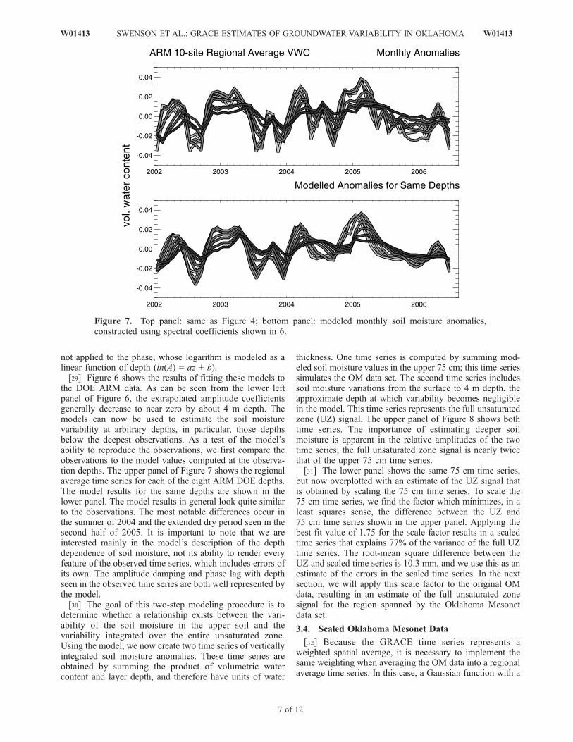
not applied to the phase, whose logarithm is modeled as alinear function of depth (ln(A) = az + b).[29] Figure 6 shows the results of fitting these models to

the DOE ARM data. As can be seen from the lower leftpanel of Figure 6, the extrapolated amplitude coefficientsgenerally decrease to near zero by about 4 m depth. Themodels can now be used to estimate the soil moisturevariability at arbitrary depths, in particular, those depthsbelow the deepest observations. As a test of the model’sability to reproduce the observations, we first compare theobservations to the model values computed at the observa-tion depths. The upper panel of Figure 7 shows the regionalaverage time series for each of the eight ARM DOE depths.The model results for the same depths are shown in thelower panel. The model results in general look quite similarto the observations. The most notable differences occur inthe summer of 2004 and the extended dry period seen in thesecond half of 2005. It is important to note that we areinterested mainly in the model’s description of the depthdependence of soil moisture, not its ability to render everyfeature of the observed time series, which includes errors ofits own. The amplitude damping and phase lag with depthseen in the observed time series are both well represented bythe model.[30] The goal of this two-step modeling procedure is to

determine whether a relationship exists between the vari-ability of the soil moisture in the upper soil and thevariability integrated over the entire unsaturated zone.Using the model, we now create two time series of verticallyintegrated soil moisture anomalies. These time series areobtained by summing the product of volumetric watercontent and layer depth, and therefore have units of water

thickness. One time series is computed by summing mod-eled soil moisture values in the upper 75 cm; this time seriessimulates the OM data set. The second time series includessoil moisture variations from the surface to 4 m depth, theapproximate depth at which variability becomes negligiblein the model. This time series represents the full unsaturatedzone (UZ) signal. The upper panel of Figure 8 shows bothtime series. The importance of estimating deeper soilmoisture is apparent in the relative amplitudes of the twotime series; the full unsaturated zone signal is nearly twicethat of the upper 75 cm time series.[31] The lower panel shows the same 75 cm time series,

but now overplotted with an estimate of the UZ signal thatis obtained by scaling the 75 cm time series. To scale the75 cm time series, we find the factor which minimizes, in aleast squares sense, the difference between the UZ and75 cm time series shown in the upper panel. Applying thebest fit value of 1.75 for the scale factor results in a scaledtime series that explains 77% of the variance of the full UZtime series. The root-mean square difference between theUZ and scaled time series is 10.3 mm, and we use this as anestimate of the errors in the scaled time series. In the nextsection, we will apply this scale factor to the original OMdata, resulting in an estimate of the full unsaturated zonesignal for the region spanned by the Oklahoma Mesonetdata set.

3.4. Scaled Oklahoma Mesonet Data

[32] Because the GRACE time series represents aweighted spatial average, it is necessary to implement thesame weighting when averaging the OM data into a regionalaverage time series. In this case, a Gaussian function with a

Figure 7. Top panel: same as Figure 4; bottom panel: modeled monthly soil moisture anomalies,constructed using spectral coefficients shown in 6.


7 of 12

W01413

halfwidth of 300 km, centered on the mean coordinates ofthe Mesonet stations is used. Figure 1 shows the contours ofthe averaging kernel amplitude. This halfwidth was chosento keep the averaging kernel localized about the OMnetwork, while still suppressing the higher degree errorsin the filtered GRACE coefficients. After averaging the soilmoisture data into monthly anomalies, the time series islow-pass filtered in the same way as the GRACE timeseries, and scaled using the factor derived in the precedingsection. This scaled time series is then removed from theGRACE total water storage time series to obtain a residualregional average groundwater estimate.

4. Results

[33] The upper panel of Figure 9 shows the time series ofmonthly GRACE total water storage anomalies (circles), aswell as the seasonal time series (line). The mean standarderror in the monthly estimates, which includes measurementerror, errors induced by the decorrelation filter, and errors inthe fields used to model and remove the atmospheric gravitysignal, is 11.4 mm. Plotted in the middle panel of Figure 9are the original (0–75 cm) and scaled (0–4 m) OM soilmoisture anomalies and seasonal time series. The bottompanel of this figure compares the GRACE and scaled OMtime series. The phase of the GRACE and OM time seriesagree quite well, both peaking around February/March and

reaching a minimum near August/September. The amplitudeof the GRACE time series ranges from about 100–150 mmpeak-to-peak, or 1.2 to 1.7 times the scaled OM time seriesamplitude.[34] By removing the scaled OM soil moisture time series

from the GRACE total water storage time series, we obtaina residual time series describing regional groundwatervariations. The upper panel of Figure 10 shows the monthlyand seasonal GRACE-OM groundwater time series. Weassume that the errors in the GRACE and scaled OM timeseries are uncorrelated, resulting in a total error of 15.3 mmin the monthly values. The peak amplitude generally occurslater than either the GRACE or OM time series by 4–6 weeks. The peak-to-peak amplitude is comparable to thatof soil moisture, ranging from 40 to 80 mm. This partition-ing of the total water storage nearly equally between soilmoisture and groundwater is consistent with water balancestudies of Illinois [Rodell and Famiglietti, 2001; Swensonet al., 2006].[35] The middle panel of Figure 10 represents our best

effort at confirming the results shown in the upper panel.Because neither the USGS nor the Oklahoma Water Resour-ces Board (OWRB) actively monitor more than a few wellson timescales shorter than a year, it is difficult to obtain welllevel data within the region spanned by the OklahomaMesonet. However, by including wells from neighboringstates, it is possible to make a rough estimate of the

Figure 8. Top panel: modeled regional average time series of monthly total soil moisture anomalies.Black line computed from only depths of 75 cm and shallower, gray line computed from depth from 0 to4 m. Bottom panel: Black line is the same as above, gray line computed by scaling 0–75 cm result (blackline) to fit 0–4 m result (top panel gray line) via least squares. X axis is time, in years, and y axis isvolumetric water content, in per cent.

8 of 12


groundwater variations averaged over a larger region. Fromthe USGS database, well level data were found for Okla-homa (5 wells), Northern Texas (19 wells), Southern Kansas(5 wells), and Western Arkansas (10 wells). Figure 2 showsthe locations of these sites. One reason for the relativelysmall number of sites having usable well level data is theneed for an estimate of the material composition or geologicformation where the well is located; this information canthen be used to assign a value of specific yield, which isnecessary to convert well level to water storage, to eachwell. Another constraint is the requirement that the dataspan some part of the period 2002 to the present. Thevarying time periods of these time series further necessitatedthe removal of temporal trends that would otherwise causespurious offsets in the regional average.[36] The thin lines shown in the middle panel of Figure 10

show groundwater storage estimated from the �40 USGSwell levels in the region around Oklahoma, scaled by theweight of the GRACE averaging kernel shown in Figure 1used to create the regional average. The circles show themonthly anomalies of the regional average; the thick lineshows the seasonal time series. The bottom panel ofFigure 10 compares the two groundwater estimates. Thewell level groundwater time series (dark gray line) appearsto confirm the general characteristics of the regionalgroundwater signal estimated as a residual from GRACE(light gray line). Both time series show a mainly seasonalcycle, and the phases of the time series agree well, giving a

correlation coefficient is 0.89 and an RMS difference is9.1 mm.

5. Discussion and Summary

[37] Although there are significant discrepencies in bothspatial and temporal sampling between the data used tocreate the two groundwater estimates, the overall agreementis good. Both time series show similar interannual variabil-ity: a relatively dry 2004, followed by a much wetter 2005,and the 2003 signal lying between the other years. While thesmaller amplitude of the well level derived time series is notsurprising based on its larger sampling area, where signalsseparated by larger distances are likely to be less wellcorrelated, the degree of similarity perhaps is surprisinggiven the dearth of well sites within the region moststrongly sampled by both GRACE and the OM network.This may indicate that variations in both soil moisture andgroundwater are well correlated at scales even larger thanthat examined here. The correlation between month-to-month changes in the two time series may also indicatethat the method for estimating GRACE uncertainty is overlypessimistic, and that some of the monthly (non-seasonal)variability should be in fact interpreted as real signal, thusdecreasing the GRACE error estimate.[38] The model used to extrapolate the DOE ARM soil

moisture observations to greater depths is simple andempirical. Physically based models for flow through porousmedia, such as the USGS VS2DI model [Hsieh et al., 2000]

Figure 9. Top panel: GRACE regional average time series of total water storage anomalies. Circlesrepresent monthly values, line represents seasonally varying values. Middle panel: monthly OMunsaturated zone soil moisture anomalies. Black circles represent 0–75 cm values, gray circles representscaled 0–4 m values. Bottom panel: comparison of GRACE and scaled OM time series. X axis is time, inyears; y axis is water equivalent thickness, in mm.


9 of 12

W01413

could also be used for this purpose. However, such modelsrequire forcing data (e.g., infiltration, evaporation, plant-transpiration), site-specific information regarding hydraulicproperties of the media, and functional relationships be-tween moisture content, saturated hydraulic conductivity,and pressure head. Because we are ultimately interested in asimple scaling relationship between the available observa-tions and the total unsaturated zone signal at those sites, thebenefit of using sophisticated models may be small.[39] The value of the scaling factor derived here (1.75)

depends on both the vertical sampling and the climate, soil,and vegetation characteristics of the Oklahoma Mesonet andDOE/ARM soil moisture networks, and therefore may notapply elsewhere. The method we have described, however,is general, and can be used to extend data sets or synthesizedata sets having insufficient vertical resolution, such as theOM, with those having insufficient lateral resolution, suchas the DOE/ARM network. Furthermore, the result that over40% of the variability in unsaturated zone water storageoccurs below the deepest OM sensors should provide a noteof caution to those who wish to use these and other soilmoisture observations in water balance studies and/or inconjunction with GRACE data; failing to account for theentire unsaturated soil moisture signal will degrade aresidual groundwater estimate much more than the errorsin the data.[40] When extensive in situ observations capable of

resolving the upper soil depths are not available, physicallybased models may be the best means to estimate soil

moisture variability in the unsaturated zone. For example,remotely sensed soil moisture in the upper few cm of soilfrom microwave instruments such as The Advanced Micro-wave Scanning Radiometer - Earth Observing System(AMSR-E) sensor aboard NASA’s Aqua satellite (launched2002) [Njoku et al., 2003] or ESA’s Soil Moisture andOcean Salinity (SMOS) mission (planned for 2008 launch)[Kerr et al., 2000] may help constrain unsaturated zoneporous media flow models. The combination of these modelsimulations of the unsaturated zone could then be combinedwith GRACE to provide regional estimates of groundwatervariability all over the globe.[41] Given the rising demands on the Earth’s freshwater

resources by an ever increasing human population, ques-tions exist on our ability to meet these demands in the future[Dennehy, 2005]. To better assess and manage groundwatersupplies, there is a strong need to improve monitoring ofthese resources, especially at the regional scale [NRC,2000]. Aquifer depletion occurs not just in arid regions,but in any location where they are overstressed. Althoughwell-level measurements are the principal source of infor-mation on the hydrologic stresses felt by aquifers, water-level monitoring in the United States is fragmented andstable networks of monitoring wells exist only in somelocations. Monitoring often occurs in individual states, butaquifers that cross boundaries are not subject to coordinatedstudy [Bartolino and Cunningham, 2003]. Furthermore,similar to the state of surface discharge observations,[Alsdorf and Lettenmaier, 2003] there has been an ongoing

Figure 10. Top panel: regional average time series of residual groundwater storage anomalies,computed by subtracting scaled OM time series from GRACE time series. Circles represent monthlyvalues, line represents seasonally varying values. Middle panel: monthly groundwater anomalies,computed from USGS well level observations. Thin gray lines represent individual wells, thick gray linerepresents regional average. Bottom panel: comparison of GRACE-OM and USGS groundwater timeseries. X axis is time, in years; y axis is water equivalent thickness, in mm.

10 of 12


decrease in the number of observing wells, both nationallyand globally [Taylor and Alley, 2001].[42] Many of the obstacles to monitoring water resources

at a variety of spatial and temporal scales may be potentiallyovercome through the application of remotely sensed mea-surements. In this study, we have combined regional totalwater storage anomalies estimated from GRACE with in situsoil moisture observations from the Oklahoma Mesonet andDOE ARM network to derive a monthly time series ofgroundwater variations spatially averaged over an area ofabout 280,000 km2. This large-scale estimate complementsthe point estimates obtained from individual observationwells, which are subject to considerable spatial heterogeneity.

[43] Acknowledgments. We wish to thank the two reviewers and theassociate editor for their constructive comments. This work was partiallysupported by NASA grant NNG04GF02G and NSF grant EAR-0309678 tothe University of Colorado, and NASA grants NNG04GE99G and REA-SoN award JPL-1259524 to the University of California at Irvine.[44] The installation of the Oklahoma Mesonet’s soil moisture sensors

was made possible, in part, by an NSF-EPSCOR grant (Project NumberEPS9550478) and an NSF MRI grant (ATM-9724594). Continued fundingfor maintenance of the network is provided by the taxpayers of the State ofOklahoma. In addition, support from the NOAA Office of Global Programs(NOAA grant number NA17RJ1227) was instrumental in the developmentof research-quality data sets.

ReferencesAlsdorf, D., and D. Lettenmaier (2003), Tracking fresh water from space,Science, 301, 1485–1488.

Arya, L. M., and J. F. Paris (1981), A physicoempirical model to predict thesoil moisture characteristic from particle-size distribution and bulk den-sity data, Soil Sci. Soc. Am. J., 45, 1023–1030.

Bartolino, J. R., and W. L. Cunningham (2003), Ground-water depletionacross the nation, U.S. Geological Survey Fact Sheet-103-03.

Basara, J. B., and T. M. Crawford (2000), Improved installation proceduresfor deep layer soil moisture measurements, J. Atmos. Oceanic Technol.,17, 879–884.

Becker, M. W. (2006), Potential for satellite remote sensing of groundwater,Ground Water, 44, 306–318.

Brock, F. V., K. C. Crawford, R. L. Elliott, G. W. Cuperus, S. J. Stadler,H. L. Johnson, and M. D. Eilts (1995), The Oklahoma Mesonet: Atechnical overview, J. Atmos. Oceanic Technol., 12, 5–19.

Crowley, J. W., J. X. Mitrovica, R. C. Bailey, M. E. Tamisiea, and J. L.Davis (2006), Land water storage within the Congo Basin inferred fromGRACE satellite gravity data, Geophys. Res. Lett., 33, L19402,doi:10.1029/2006GL027070.

Dennehy, K. F. (2005), Ground-water resources program, U.S. GeologicalSurvey, Fact Sheet 2005-3097.

Entin, J. K., A. Robock, K. Y. Vinnikov, S. E. Hollinger, S. Liu, andA. Namkai (2000), Temporal and spatial scales of observed soilmoisture variations in the extratropics, J. Geophys. Res., 105,11,865–11,877.

Hirabayashi, Y., T. Oki, S. Kanae, and K. Musiake (2003), Application ofsatellite-derived surface soil moisture data to simulating seasonal preci-pitation by a simple soil moisture transfer method, J. Hydromet., 4, 929–943.

Hollinger, S. E., and S. A. Isard (1994), A soil moisture climatology ofIllinois, J. Clim., 7(5), 822–833.

Hsieh, P. A., Wingle, William, and R. W. Healy (2000), VS2DI–A graphi-cal software package for simulating fluid flow and solute or energytransport in variably saturated porous media: U.S. Geological SurveyWater-Resources Investigations Report 99-4130, 16 p.

Hutson, S. S., N. L. Barber, J. F. Kenny, K. S. Linsey, D. S. Lumia, andM. A. Maupin (2004), Estimated use of water in the United States in2000, USGS Circular 1268.

Illston, B. G., J. B. Basara, D. K. Fisher, C. Fiebrich, K. Humes, R. Elliott,K. C. Crawford, and E. Hunt (2007), Mesoscale monitoring of soilmoisture across a statewide network, Submitted to the J. Atmos. andOceanic Tech.

Kelly, R. E. J., A. T. C. Chang, J. L. Foster, and D. K. Hall (2004), Usingremote sensing and spatial models to monitor snow depth and snow

water equivalent, in R. E. J. Kelly, N. A. Drake, and S. Barr (Eds.)Spatial Modelling of the Terrestrial Environment, Chichester: John Wileyand Sons Ltd.

Kerr, Y. H., J. Font, P. Waldteufel, and M. Berger (2000), The Soil Moistureand Ocean salinity Mission -:SMOS Earth Observation Quarterly, 2000,pp. 18-26.

McPherson, R. A., et al. (2007), Statewide monitoring of the mesoscaleenvironment: A technical update on the Oklahoma Mesonet, J. Atmos.Oceanic Technol., in press.

National Research Council (2000), Investigating groundwater systems onregional and national scales, National Academy Press, Washington, D. C.,143 p.

Njoku, E. G., T. L. Jackson, V. Lakshmi, T. Chan, and S. V. Nghiem (2003),Soil moisture retrieval from AMSR-E, IEEE Trans. Geosci. RemoteSens., 41(2), 215–229.

Peltier, W. R. (1996), Mantle viscosity and ice-age ice sheet topography,Science, 273, 1359–1364.

Peltier, W. R. (2004), Global glacial isostasy and the surface of the Ice-AgeEarth: The ICE-5G (VM2) model and GRACE, Ann. Rev. Earth Planet.Sci., 32, 111–149.

Rodell, M., and J. S. Famiglietti (2001), Terrestrial water storage variationsover Illinois: Analysis of observations and implications for Gravity Re-covery and Climate Experiment (GRACE), Water Resour. Res., 37(5),1327–1340.

Rodell, M., J. S. Famiglietti, J. Chen, S. Seneviratne, P. Viterbo, S. Holl,and C. R. Wilson (2004), Basin scale estimates of evapotranspirationusing GRACE and other observations, Geophys. Res. Lett., 31,L20504. doi:10.1029/2004GL020873.

Rodell, M., J. Chen, H. Kato, J. Famiglietti, J. Nigro, and C. Wilson (2006),Estimating groundwater storage changes in the Mississippi River basin(USA) using GRACE,Hydrogeology J., doi:10.1007/s10040-006-0103-7.

Schmidt, R., et al. (2006), GRACE observations of changes in continentalwater storage, Global Planet. Change, 50, 112–126.

Schneider, J. M., D. K. Fisher, R. L. Elliott, G. O. Brown, and C. P.Bahrmann (2003), Spatiotemporal variations in soil water: First resultsfrom the ARM SGP CART network, J. Hydromet., 4, 106–120.

Seo, K. W., C. R. Wilson, J. S. Famiglietti, J. L. Chen, and M. Rodell(2006), Terrestrial water mass load changes from gravity recovery andclimate experiment (GRACE), Water Resour. Res., 42, W05417,doi:10.1029/2005WR004255.

Shah, T., D. Molden, R. Sakthivadivel, and D. Seckler (2000), The globalgroundwater situation: Overview of opportunities and challenges.Colombo, Sri Lanka: International Water Management Institute.

Swenson, S., and J. Wahr (2002), Methods for inferring regional surface-mass anomalies from GRACE measurements of time-variable gravity,J. Geophys. Res., 107(B9), 2193, doi:10.1029/2001JB000576.

Swenson, S., and J. Wahr (2006a), Estimating large-scale precipitationminus evapotranspiration from GRACE satellite gravity measurements,J Hydrometeorol., 7, 252–270.

Swenson, S., and J. Wahr (2006b), Post-processing removal of correlatederrors in GRACE data, Geophys. Res. Lett., 33, L08402, doi:10.1029/2005GL025285.

Swenson, S., J. Wahr, and P. C. D. Milly (2003), Estimated accuracies ofregional water storage variations inferred from the Gravity Recovery andClimate Experiment (GRACE), Water Resour. Res., 39(8), 1223,doi:10.1029/2002WR001808.

Swenson, S. C., P. J.-F. Yeh, J. Wahr, and J. S. Famiglietti (2006),A comparison of terrestrial water storage variations from GRACE with insitu measurements from Illinois, Geophys. Res. Lett., 33, L16401,doi:10.1029/2006GL026962.

Syed, T. H., J. S. Famiglietti, J. Chen,M. Rodell, S. I. Seneviratne, P. Viterbo,and C. R. Wilson (2005), Total basin discharge for the Amazon and Mis-sissippi River basins from GRACE and a land-atmosphere water balance,Geophys. Res. Lett., 32, L24404, doi:10.1029/2005GL024851.

Tamisiea, M. E., E. W. Leuliette, J. L. Davis, and J. X. Mitrovica (2005),Constraining hydrological and cryospheric mass flux in southeasternAlaska using space-based gravity measurements, Geophys. Res. Lett.,32(20), L20501, doi:10.1029/2005GL023961.

Tapley, B. D., S. Bettadpur, J. C. Ries, P. F. Thompson, and M. M. Watkins(2004), GRACE measurements of mass variability in the Earth system,Science, 305, 503–505.

Taylor, C. J., and W. M. Alley (2001), Ground-Water-Level Monitoring andthe Importance of Long-Term Water-Level Data, U.S. Geological Survey1217.

Velicogna, I., and J. Wahr (2006), Measurements of time-variable gravityshow mass loss in Antarctica, Science, 311, 1754–1756.


11 of 12

W01413

Wahr, J., M. Molenaar, and F. Bryan (1998), Time variability of the Earth’sgravity field: Hydrological and oceanic effects and their possible detec-tion using GRACE, J. Geophys. Res., 103(B12), 30,205–30,229.

Wahr, J., S. Swenson, V. Zlotnicki, and I. Velicogna (2004), Time-variablegravity from GRACE: First results, Geophys. Res. Lett., 31, L11501,doi:10.1029/2004GL019779.

Wahr, J., S. Swenson, and I. Velicogna (2006), Accuracy of GRACE massestimates, Geophys. Res. Lett., 33, L06401, doi:10.1029/2005GL025305.

Wu, W., M. A. Geller, and R. E. Dickinson (2002), The Response of SoilMoisture to Long-Term Variability of Precipitation, J Hydromet, Vol. 3,No. 5 pp. 604-613.

Yeh, P. J.-F., S. C. Swenson, J. S. Famiglietti, and M. Rodell (2006),Groundwater storage changes inferred from the Gravity Recovery and

Climate Experiment (GRACE), Water Resour. Res., 42, W12203,doi:10.1029/2006WR005374.

��J. Basara, Oklahoma Climatological Survey, University of Oklahoma,

Norman, OK, USA.

J. Famiglietti, Department of Earth System Science, University ofCalifornia, Irvine, CA, USA.

S. Swenson, Advanced Study Program, National Center for AtmosphericResearch, Boulder, CO, USA. ([email protected])

J. Wahr, Department of Physics and CIRES, University of Colorado,Boulder, CO, USA.

12 of 12


estimating profile soil moisture and groundwater variations using grace...

Documents