CE

UeT

DC

olle

ctio

n

ESTIMATING LABOR SUPPLY IN ALBANIA

ByGisela Shameti

Submitted toCentral European UniversityDepartment of Economics

In partial fulfillment of the requirements for the degree ofMaster of Arts

Supervisor: Professor Peter Grajzl

Budapest, Hungary2008

CE

UeT

DC

olle

ctio

n

ii

Abstract

Estimating labor supply in Albania is interesting not only from an econometrical point of view

but it is mainly important for policy making in the field of labor market. Using the data from the

Living Standard Measurement Surveys in Albania covering the period from 2002 to 2005, this

paper studies the labor force participation changes in the Albanian labor market and, focusing

on the 2003-2004 period, estimates labor supply, correcting for selectivity bias via the Heckman

procedure. Drawing on these samples, it is evident that labor participation rates in Albania

declined from 2002 to 2005 both in terms of age cohorts and in terms of gender. Female

participation shows a continuous decline, as does the participation of older generations. The OLS

results over 2003 and 2004 samples indicate small positive wage elasticity of 0.08 and 0.06,

respectively. The results are nevertheless subject to many procedural and methodological

limitations. When correcting for exogeneity and selectivity bias through Heckman procedure on

these datasets wage elasticities became 0.23 and 0.12 confirming labor supply theory and getting

closer to worldwide trends. However, the other variables in the equation proved insignificant

suggesting various problems with data, like measurement error, exogeneity or multicollinearity.

The paper suggests ways for further work on the topic.

CE

UeT

DC

olle

ctio

n

iii

AKNOWLEDGEMENTS

First of all, I would like to thank my supervisor, Professor Grajzl, for his valuable

suggestions and the strong encouragement he gave me for concluding my work. Special

thanks go to Prof. Korosi, Prof. Teledgy and Prof. Kezdi for their econometric advises

regarding my thesis. An indispensable contribution to my work was made by the

Albanian Ministry of Labor and Equal Opportunities which provided me with a lot of

information about the Albanian labor market and to whom I am really indebted. And last

but not least, I would like to thank my parents and family who always supported and had

faith in me.

CE

UeT

DC

olle

ctio

n

iv

Table of Contents

ESTIMATING LABOR SUPPLY IN ALBANIA ..................................... i

1. Introduction......................................................................................... 1

2. The Structure of the Albanian Labor Market after the 1990s.......... 4

3. Empirical Framework......................................................................... 7

4. Data Summary ...................................................................................11

5. Estimation Results..............................................................................16

6. Conclusion ..........................................................................................25

APPENDIX ...............................................................................................27

A1.List of Major Occupations (ISCO-1988) ..............................................................27

A2.List of Variable Definition ...................................................................................28

A3. TABLES.............................................................................................................29

REFERENCES .........................................................................................33

CE

UeT

DC

olle

ctio

n

1

1. INTRODUCTION

The fall of communism in Albania in 1991 was followed by many economic,

social and demographic changes. All the sectors experienced huge structural

modifications through their transformation from a state of command economy to a market

economy. The labor market constitutes a very important element of this transformation,

representing that vital part determining an economy’s development and growth. While it

is a well known fact that the Albanian labor market, due to the political and economic

changes, as any other transitional economy, went through essential shocks like huge

initial unemployment, drastic declines in labor force participations (LFP), new job

reorganization, emigration, etc., systematic empirical analyses of Albanian labor market

are scant.

The many reasons for this lack of systematical empirical analysis include the non-

availability of data (especially before 2000), huge informal sector, emigration and

missing international surveys undertaken in the country. Only a few attempts on

quantifying each of these are existent like, for example, Muço et al. (2004) who works on

the movements of the Albanian labor market, trying to assess the size of the informal

market, or Kule et al. (2002), who working on micro-data tries to identify the causes and

consequences of emigration, a widespread phenomenon in Albania after the 1990s. Many

other labor market reports from the World Bank, Albanian Ministry of Labor and Equal

Opportunities, Albanian Institute of Statistics, United Nations Development Programme

(UNDP) and International Labor Organization (ILO) only give a general picture of the

Albanian labor market. However, to the best of my knowledge, there exists no systematic

econometric study done on the trends of Albanian workers’ labor supply and the

CE

UeT

DC

olle

ctio

n

2

determination of the uncompensated, compensated wage elasticity and income elasticity.

Studies on this topic would be particularly interesting for the case of transitional Albania,

a country whose GDP has been one of the lowest in Europe for a considerable time frame

now and for which the development of the labor market constitutes one of the primary

objectives of each and every political party in power after the 1990s.

This paper, therefore, tries to identify the movements and trends in the Albanian

labor market from 2002 to 2005 and estimate labor supply elasticity for different subsets.

Unfortunately, due to the non-availability of the necessary data, compensated wage

elasticity and income elasticity cannot be estimated, only the uncompensated one1.

However, knowing the average labor response of the Albanian employees, captured by

uncompensated wage elasticity, is not only informational from an applied econometrics

point of view and a checking exercise for how the Albanian labor market fits into the

whole world labor supply theory but it can be mostly applicable by labor market policy

makers in constructing the most adapt policies fitting into the Albanian environment.

This is beneficial especially in the case of Albania, one of the poorest countries in Europe

and a country where the Vocational Education and Training (VET) system, a crucial

program for improving human capital, has been experiencing a dramatic deterioration

(ILO, 2003-2004). Therefore, this study, although encountering different technical

caveats working on the Albanian Panel Surveys of 2003 and 2004, estimates

uncompensated wage elasticity, first, by simple Ordinary Least Squares (OLS), and

second, by the two-step Heckman procedure, which corrects for selectivity bias and

exogeneity.

1 The uncompensated wage elasticity is defined as the percentage change in hours worked as a result of aone percentage change in the net hourly wage. This elasticity is broken into substitution effect:compensated (for income changes) elasticity and income effect: income elasticity.

CE

UeT

DC

olle

ctio

n

3

The thesis is organized as follows: Section 2 describes the situation of the

Albanian labor market from 2002 till 2005, Section 2 gives a theoretical background,

Section 4 is dedicated to data description, followed by regression results and

interpretation in Section 5. Section 6 concludes.

CE

UeT

DC

olle

ctio

n

4

2. THE STRUCTURE OF THE ALBANIAN LABORMARKET AFTER THE 1990S

After the 1990s, Albania went through many radical economic, social and

demographic changes. During the whole period of transition, which is not over yet, it has

experienced many ups and downs in terms of economic growth, structural changes and

macroeconomic stability, and the labor market was not an exception to this. Albania

currently has a young age structure, with almost half of the population being under 25

years, but with the tendency to decline in the future (ILO, 2006). One possible reason for

this can be the fact that since the collapse of communism, the Albanian population has

been decreasing rapidly due to large-scale emigration and falling birth rates. 600,000-

800,000 people (mostly men) are working abroad, mainly in Greece and Italy (EIU,

2004).

After restructuring in the early 1990s, labor force participation rates fell by 18%

points for the period 1991-2002, and since 2000 less than two thirds of the working age

population is actively participating in the labor market (INSTAT, 2002). The decline has

been higher for women, for whom only 50% of the working age population is active in

the labor market. This decline may be explained by various factors, including

engagement in the informal sector, which is not recorded, discouragement and dropping

out of the labor force or problems coming from the economic transformation and

industrial restructuring in terms of available jobs suitable for certain population with

certain sets of qualifications (ILO, 2006). Due to the mass privatization of state-owned

enterprises, Albania experienced a huge drop of employment in the public sector, and the

industrial sector, with only the service sector keeping good rates of employment. Two

CE

UeT

DC

olle

ctio

n

5

thirds of all employees till 2002 were employed in private agriculture, which makes

agriculture the largest sector in the country.

For women the decline was more pronounced because besides the overall changes

hitting the Albanian labor market, they were more exposed to the lack of childcare (in

2003 the number of kindergartens fell by 60% in urban areas) (INSTAT, 2004),

consequently prohibiting them from participating as equally as men in the labor market.

Another very important factor which is usually claimed to explain the higher decline is

related to the male mass emigration, which leaves the wives at home taking care of their

children, engaging in housework or informal market and thereby decreasing their

working hours out of the house. One would expect male emigration to open more

vacancies for women; however, the higher decline in female labor supply and also the

much lower share of women holding full-time jobs suggests that either these positions did

not exist in the first place (as a consequence of which males emigrated) or females moved

to the informal market, a measurement of which is still not available for a country as

Albania.

Many of the firms, enterprises and employees in Albania operate in the shadow or

informal market. Studies on the size of the Albanian informal market conclude that it is

mainly supported by remittance flows from emigrants living in the neighboring countries,

which most of the time are also channeled through the informal currency market,

therefore not possible to be measured in size and/or frequency. IMF reports of 2003 claim

that the informal sector should be between 30 and 60 percent, with a higher chance of it

being close to 60 (Muço et al., 2004). However, the unemployment rate measured by the

General Census, 2001 was 22.7%, while the registered unemployment rate according to

CE

UeT

DC

olle

ctio

n

6

Bank of Albania was 16.4% (Muço et al., 2004). Therefore, it is very important to

mention that the quality of data and the accuracy with which they were gathered is

limited. In a survey conducted by the Albanian Ministry of Labor in 1996, about 65%-

70% of individuals working in the private sector were not officially recorded, and

Albania first conducted a Labor Force Survey only in 2007. A lot of information is

missing and the only available source of it is the Albanian Institute of Statistics. The size

of the gap between the actual economic parameters and the published numbers cannot be

accurately quantified, but according to Muço et al. (2004), it is around 10% of the total

employment.

CE

UeT

DC

olle

ctio

n

7

3. EMPIRICAL FRAMEWORK

Labor market participation influences and determines the development and the

performance of a country’s labor market, which by itself constitutes a key sector of the

market economy. Labor market participation can be measured in two ways: by the

presence of the workers in the labor market and actually working in it (usually estimated

by a conditional logit econometric method) or alternatively by the number of hours,

depending on many factors, one decides to supply to the labor market. The factors that

establish labor market participation have always been numerous and varying from person

to person, across genders, from a different age group to another age group and from

country to country. The most common ones among those factors are own-income,

individual characteristics like education, age, gender, family content, geographical

characteristics and many others.

Historically, the difference in labor supply is particularly exhibited between males

and females, with the latest world trends showing that male labor participation has

declined, while female labor supply has increased significantly. (Bosworth et. al., 1996)

However, according to Killingsworth (1983), despite the labor supply upward trend,

female participation has increased more in part-time jobs than in full time, showing once

more that factors such as the existence of small children, childcare, presence and help of

the spouse, etc. are more influential when it comes to female labor participation. In terms

of uncompensated wage elasticity, international research suggests values which vary

from -0.23 to -0.05 for males and 0.6 to 1.1 for females (Killingsworth, 1983).

CE

UeT

DC

olle

ctio

n

8

In particular, the neo-classical approach of consumer theory states that the number

of hours a person supplies in the labor market is derived by solving the first-order

conditions of the household utility maximization problem, where the utility function is

assumed to be the standard and well-behaved one. That is, following Lokshin (2004), a

consumer maximizes utility:

(1) Uijt = jXit + jYijt + ijt

where Uijt is utility of household i choosing state j at time t (j presents different states in

the labor market, like employed, unemployed, out of the labor force etc.), Xit is the vector

of household characteristics that impact household’s choice at time t, Yijt contains the

outcome variables from choosing state j, like wage, social assistance, etc., and are

vectors of unknown parameters and ijt is a random disturbance, including unobservable

factors. The probability that household i chooses j at time t is given by:

(2) Prit(j) = Pr [Uijt > Uiqt]

= Pr[ ijt - iqt > Xit qit - jit ) + Yjit qit - jit )] for any j q

In order to estimate the intertemporal elasticity of labor supply, one has to look at the

labor supply function, which is given by a homogenous-of-degree-zero function of wage

or labor income(i), the price of a basket of consumption goods (p) and non-labor income

(V):

(3) H= H( i, p, V)

with explicit functional form adopted looking like:

(4) log (Hi ) = 0 + 1log(w/p)i + 2log(V/p)i + 3Xi + i

CE

UeT

DC

olle

ctio

n

9

where again Xi is the vector of individual characteristics and i random error. In cross-

section samples, p is assumed to be the same to all individuals and is dropped out of the

model.

Wage elasticities are then given by a transformation of the Slutsky decomposition

of the wage effect into substitution and income effect:

(5) ( H/ w)(w/H) = ( H/ w)u=const (w/H) + (w/H) H( H/ V)

where the left hand side refers to the uncompensated wage elasticity, which is further

broken into: the substitution effect (the first term on the right), also known as

compensated wage elasticity, and income effect (the second term on the right), also

known as marginal propensity to earn. Referring to the semi-log specification in equation

(4), the uncompensated wage elasticity is given by 1, the income elasticity is given by 2

and compensated wage elasticity by 1 – (wH/V) 2. According to the classical theory, 1

is expected to be positive (higher wage results in higher number of hours) and 2

negative, resulting in a C-shaped (backward-bending) labor supply curve (Robins, 1930).

The usual problem that is encountered when estimating labor supply is the way

hourly wages are imputed into the equation, since there is no unique rate for measuring

that in practice. Usually for salaried workers, the hourly wage is computed as the salary

divided by the standard amount of hours per time period, which obviously induces

measurement error and a negative correlation between hours and wages, which

consequently creates a downward bias for the wage coefficient. One way to deal with this

error is through instrumenting wage by age, education and other similar parameters that

might influence it. However, in order for the estimate to be consistent, the instrumental

variables for wage should be exogenous, i.e they should not reflect the person’s taste for

CE

UeT

DC

olle

ctio

n

10

work, a condition which cannot be easily achieved. Moreover, such exercises also suffer

from sample selection or selectivity bias: the wages of non labor participants cannot be

observed and therefore, the labor supply is fit only to the participants.

A standard way to deal with these two problems simultaneously is via the

Heckman procedure (Heckman, 1980) according to which, the following equations are

estimated:

(6) LFPi = 0 + 1ln(w)i + 2Xi1 + i

(7) log(w)i = 1 Xi1+ 2 Xi2 i + ui where i = X`i) / F( X`i ) ;

(8) log(Hi ) = 0 + 1log( )i + 2Xi2 + ˆ+ i

where the first one, a probit equation also known as the selection equation which

measures the probability of participation, includes all observations and singles out

participants from nonparticipants. The estimates of this equation are then used to create

- the inverse Mills ratio, which captures this selection and introduces it to the wage

equation applicable only to the participants. The last stage of the procedure estimates

labor supply using the predicted wages from equation (7). Xi2 includes personal

characteristics that influence wages but not labor force participation, so that the predicted

values of wage are not perfectly collinear with the regressors of hours equation (El-

Hamidi, 2003). In this manner, both sample selection and exogeneity are taken care of.

The structure of the dataset which is used from this paper, however, does not allow us to

apply this method to each and every year.2 Therefore, after analyzing analytically the

moves in the Albanian labor market participation from 2002 till 2005, the

abovementioned procedure will be applied only to the 2003 and 2004 data.

2 In datasets of 2002 and 2005, no unique identification number is present therefore the merging ofdifferent tables was impossible. The 2003 and 2004 datasets do not have this problem.

CE

UeT

DC

olle

ctio

n

4. DATA SUMMARY

This study takes into consideration the results of four Living Standards

Measurement Surveys (LSMS) that were undertaken in Albania between 2002-2005.

These multi-purpose surveys are generally used as a useful source of information for

determining the living conditions of the country’s households, the poverty level and for

assisting policy-makers in their surveillance of various social programs. The household

questionnaires include information about the household members like, age, gender,

marital status, education, labor market status and various other modules including

migration, fertility, subjective poverty, agriculture and nonfarm enterprises. The LSMS of

2002 included 458 Primary Sampling Units, with a total of 3600 households covering

some of the largest cities in Albania. Based on this data set, two panel data surveys:

Albanian Panel Surveys (APS), were conducted in 2003 and 2004. The APS of 2003 was

constructed in a panel form, taking almost half of the households of 2002 (2155 out of

which 1780 were interviewed in 2002), and the panel size of the 2004 APS was the same

as the one in 2003. The LSMS of 2005 followed rigorously the structure and the notations

used by LSMS of 2002, including 1800 panel household units and 3600 new households

(WORLD BANK, 2008). According to the World Bank publications on the main labor

market indicators based on these surveys, during 2002-2005, the labor force participation

rate fell from 65.2% in 2002 to 63.7 % in 2004, due to which unemployment rate fell

from 10.2% to 5.6%.(Carletto et al., 2005). One possible explanation for the double fall in

unemployment and labor force participation rates is the low amount of job creation in the

CE

UeT

DC

olle

ctio

n

12

Albanian labor market during this period, or the discouragement of employees, who

stopped searching for jobs and left the labor market.

Figure 1 and 2 below, drawing on these datasets, give a representation of the

changes in labor force participation by age and gender, respectively.3 The calculations for

the LFP are made based on the individuals’ responses about their presence in the labor

market, i.e labor force participation (LFP) was measured as the percentage of population

who declared to have been working during the last 7 days (as defined by ILO). Looking

at LFP by age (Figure 1), we can infer that the majority of the working population is

concentrated between 35-44 and 45-54 age cohorts, for which in each case LFP in 2005

increased. For the other age groups, however, participation decreased from 2002 to 2005.

An interesting feature of the chart is also the great amount of 15-24-year-old workers in

2002 and its sharp decline afterwards.

LFP by age

0

5

10

15

20

25

30

15-24 25-34 35-44 45-54 55-64 Above 64

Age cohorts

Popu

latio

n in

% 2002200320042005

Figure 1. LFP by age

Turning to Figure 2, the percentage of women participating in the labor market

decreased from 31% in 2002 to 26% in 2005 while an opposite trend is observed for

males, confirming our prior beliefs.

3 Table A3.1 in the Appendix gives a summary of the data sets downloaded from the World Bank classifiedby gender for each respective year

CE

UeT

DC

olle

ctio

n

13

LFP by sex

0%5%

10%15%20%25%30%35%40%45%

2002 2003 2004 2005

Years

LFP

in % Females

Males

Figure 2. LFP by gender

Although the samples do not represent the same households during these years,

there are about 1700 observations (mainly from the working age population) which are

interviewed consequently. Assuming that these samples of households are randomly

chosen year after year besides the ones kept the same, the numbers presented in the table

and by the figures remain indicative of the fall in female labor market participation.

However, a problem we have to be cautious about is that, as also suggested by the data,

there is a considerable number of individuals who claim not to work but who on the other

side work on their own account or on their own farm and for whom wages or amount of

labor supply is missing or cannot be precisely calculated. Therefore, the results obtained

here are not an indication of the whole population features but only of the ones who

declared to be working.

The careful cleaning of each of the four data sets based on LSMS-s of 2002, 2003,

2004 and 2005 resulted into fours subsets for which there are no missing data and for

every single observation age, gender, marital status, occupation, the approximate number

of hours the individual worked during the last month and the net payment per month are

available. The APS of 2003 and 2004 also gives us the possibility to extract person’s

CE

UeT

DC

olle

ctio

n

14

highest level of education attained, number of children under 6, experience measured by

the number of years the person had been working in his/her primary occupation and

health status, i.e. a self–assessment of the person’s health if his/her health is below or

above average. Tables A3.2 and Table A3.3 in the Appendix give a summary of those.

As Table A3.2 reveals, females are represented in a lower share during the four

years, indicating that either their labor participation is lower and consequently the data

for them is missing or that the data is missing because they are more involved in the

informal sector not captured by the survey. In terms of the average age, both females and

males show a stable pattern through the years, although females’ average working age is

lower than for males. The average monthly wages (around 20000 Lek or around 180

EUR) display an irregular pattern among females and males, while the average monthly

hours for females are always lower than those of males, although they seem to follow the

same trend as for males: declining initially and then going upward in 2005, surpassing the

2002 level. Figures 3 and 4 illustrate this point.

Monthly Income Trends

0

5000

10000

15000

20000

25000

2002 2003 2004 2005

Year

Wag

e (in

new

Lek

)

FemalesMales

Figure 3.Monthly income

CE

UeT

DC

olle

ctio

n

15

Monthly Hours Trends

0

50

100

150

200

2002 2003 2004 2005

Year

Aver

age

Hour

s Pe

r M

onth

FemalesMales

Figure 4. Monthly hours trends

Regarding occupation, the majority of the observations belong to group 7, group 6

and group 2 in decreasing proportions, each representing Craft and Related Trade

Workers, Skilled Agricultural and Fishery Workers and Professionals, as defined by the

International Standard Classification of Occupation (ISCO) 1988.4 86% of the sample is

married, 6% are single and a very small part of the wage earners are widowers or

divorced.

For the variables not available for all the years, we turn to Table A3.3. In terms of

health, the majority of the households are above the average level. Education level has

different representations in 2003 and 2004: in 2003 for the majority the highest level of

education is the vocational 4 to 5 years, while for 2004 nine years of schooling or

secondary general is the highest. Also in 2003, the representation of higher education

levels like university in Albania, abroad or post-graduate studies, although small in

absolute terms, compared to 2004 is much bigger. The average experience in 2003 is

around 9 years, while in 2004 it is close to 7 and there were more individuals with

children younger than six in 2004 than in 2003. Keeping in mind the characteristics of

our datasets, we proceed now to the estimation results.

4 A list of the ten major groups and their respective definition is given in the Appendix

CE

UeT

DC

olle

ctio

n

16

5. ESTIMATION RESULTS

To estimate the wage elasticities and identify the different trends across years, we

first run five different regressions: one cross-section for each particular year and then a

pooled Ordinary Least Square (OLS) for all the observations (see Table A3.4 in

Appendix). The pooled OLS is used for two reasons: first, because a panel data

regression cannot be conducted since the sample of the households for each year is

different (although 1700 observations were kept the same); and, through the data cleaning

and data mining even more observations were left out of the regressions due to missing

information; and second, because pooling the years together increases the sample size

and gives a more accurate estimate for the elasticities. Each of the first four regressions

follow equation (4), where vector Xi includes age, gender, three dummies for the marital

studies: married, single, widower with divorced as the numeraire. Education, number of

small children, health conditions should have also been included in the regressions but

since they are not available for all the years, for comparison reasons, they are left out at

this point. The pooled OLS includes three year dummies also, taking year 2002 as the

base year.

The OLS regressions presented in Table A3.4, corrected for heteroskedasticity

and run on Albanian datasets of 2002, 2003, 2004 and 2005, show that age, marital status

and wage are (statistically) significant in determining employees’ labor market

participation and the amount of hours they devote to working, with few exceptions from

one year to another. Age and gender have the expected sign and they usually behave the

same during different years. Marital status, on the other hand, comes only significant in

2002 and the signs of the estimates are negative. According to them, a married person,

CE

UeT

DC

olle

ctio

n

17

single or widower, is expected to work less than a divorced one, implying that the

absence of a spouse gives an incentive for more labor market participation. However, in

the other years these dummies have different signs and are insignificant. Obviously, the

results are highly biased not only due to selectivity and exogeneity but also omitted

variables bias, as they are a poor capture of equation (4), made evident by the very small

respective R-squares: 1%, 2%, 5% and 3%. The aim here was to look at the values of the

uncompensated wage elasticities and focus more on their trends than their actual values.

In these terms, the uncompensated wage elasticities turn out to be significant, and they

have the expected size and sign for this type of exercise. For 2002, for example, a 1%

increase in the monthly wage increases monthly working hours on average by 0.11%

(subject to the abovementioned econometric caveats). Interestingly, wage elasticity

declines during the years from 0.11 in 2002 to 0.06 in 2005, implying a labor supply

function getting more and more inelastic.

The last column of Table A3.4 gives the results of pooling the four years together.

In this regression, in addition to Xi, year dummies are included in order to capture for the

year differences. The increase in sample size did not improve our results much and, as a

matter of fact, all the variables but log wage and the year dummies are insignificant, and

therefore, the results are not that informative. For this reason, more variables were

included and two more OLS regressions on 2003 and 2004 datasets were run.

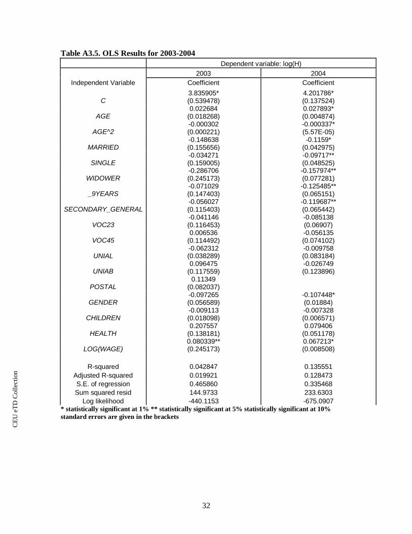
The OLS regressions on 2003 and 2004 are presented in Table A3.5, and they

include a quadratic form of age, education dummies, a health dummy (1 if the person said

their health is above average, 0 otherwise) and number of children younger than 6 in the

household. Evidently, the results ameliorated relative to the previous ones but not very

CE

UeT

DC

olle

ctio

n

18

significantly so. For example, for 2003, although many new factors, which are expected

to be important in determining one’s decision to the amount of participation in the labor

market, were added and would correct for the omitted variable bias, the estimates are still

not significant. Only wage elasticity is significant at the 5% significance level, and it

shows that, ceteris paribus, the uncompensated wage elasticity for 2003 is 0.08. The

independent variables could explain only 4% of the variation in the dependent variable,

which shows once again the big exogeneity present in the model and multicollinearity

among the dummy variables.

For 2004 the picture looks better. Age affects the labor supply positively, but after

some point it has decreasing marginal effects (the coefficient on age squared). All three

marital status dummies are also significant, and all are negative, suggesting that divorced

people (the numeraire) tend in general to work more than others, ceteris paribus, which is

consistent with the previous OLS results presented in Table A3.4. From the education

dummies only the first two, for which the highest level of education attained is 9 years

and secondary general, come out significant. The negative coefficients on them mean that

people from these education categories work more than those with no education. Number

of children under six and health status do not affect labor supply for this sample. Female

labor supply is 10% lower than for males, ceteris paribus and the uncompensated wage

elasticity is 0.06, different from the 0.08 estimated earlier and much more significant.

Although part of the omitted variable bias seems to have been taken good care of, the

problems of exogeneity and sample selection bias are still not solved. Therefore, we next

apply the two-stage Heckman procedure, which in theory is supposed to correct for those.

CE

UeT

DC

olle

ctio

n

19

Table 1 gives the results from equations (6) and (7). In the probit equation, vector

Xi1 includes age (in quadratic form), gender, a health dummy based on individuals’ health

self-assessment, education represented by three dummies measuring the highest level of

education attained by the interviewees and a variable about the number of children under

six years old present in the household. In the OLS regressions earlier education was

imputed by 9 dummies, but given that most of them come out insignificant and a lot of

multicollinearity is induced because of them, the education dummies were grouped in

groups of two, and post graduate studies dummies were left out, since these last ones

always turned out insignificant and their variance is very small. Marital status dummies

were also left out of the equation for the same reasons. In the wage equation health and

number of children are not included, making these variables in this way our exclusion

restriction, since there is no logical reasoning behind why these variables would directly

determine a person’s wage. The rest of the variables from equation (6) are kept the same,

and in addition, experience (in quadratic form), 9 dummies representing different

occupations and the inverse Mills ratio, which counts for sample selection, were added.

Looking at the probit estimates and comparing the results for 2003 and 2004, the

variables have almost the same expected signs and quite the same magnitude. In both

years, age and its quadratic form are significant and have a positive effect on the

probability of labor participation. Gender and health dummies are both significant as well

for 2003 and 2004, and as expected, females, the same with people whose health is below

average, have a lower probability of being present in the labor market than the rest of the

population, keeping everything else constant. Interestingly, the number of the children

under six does not show to have any impact on labor participation, probably due to the

CE

UeT

DC

olle

ctio

n

20

small representation of those captured by the current sample. Education also appears not

to affect this decision either and the signs of the estimates are different in 2003 and 2004.

For example, in 2003, having a secondary school as the highest level of education

increases the probability of labor force participation by 0.03, while in 2004 this

probability increases by 0.21, although insignificant. In 2003, having vocational school or

university as the highest level of education decreases this probability while in 2004 the

opposite is observed. The probit regressions pass the stability test quite significantly, but

given that many dummies are used at this stage and keeping in mind that one of the

serious problems associated with probit estimator is exogeneity, we should still be very

cautious in interpreting these results from a quantitative point of view.

Next let us look at the wage equation in Table 1, the coefficients of which across

years are very close in magnitude. The significance is not the same as for the case of

2003 when many of the variables like age, education, experience and some of the

occupations turn out insignificant. Only gender and groups 5, 6 and 9 are statistically

significant. On the contrary, in 2004 all the variables but gender are significant and,

moreover, age and experience affect wages in the same manner: they have a negative

effect as age and experience increase but after a turning point, the marginal effect is

positive. Regarding education estimates, they are all negative, implying that the people

with these highest levels of education tend to work less than those with other types of

education. The same sign is observed for most of the occupations too, indicating that

members of these groups work less than the armed forces (the numeraire). The overall

quality of the regressions is good, especially for 2004, for which the test results are more

satisfactory than for 2003. The inverse Mills ratio for 2003 turns out insignificant,

CE

UeT

DC

olle

ctio

n

21

implying that sample selection is not a problem for this sample, but for 2004 the ratio is

significant, indicating the presence of sample selection bias and supporting the validity of

the applied procedure.

Table 1. Results of Probit and Log(Wage) EquationsDependent Variable: LFPi Dependent Variable: log(W)i

2003 2004 2003 2004IndependentVariable Coefficient Coefficient Coefficient Coefficient

C-3.61655*(0.105429)

-3.49864*(0.322978)

9.547006*(3.152431)

13.45239*(0.795391)

AGE0.174285*(0.004437)

0.178064*(0.006229)

0.033983(0.094176)

-0.04757**(0.023173)

AGE^2-0.00198*(5.51E-05)

-0.00212*(7.26E-05)

-0.00043(0.001067)

0.000266**(0.000274)

EXPERIENCE-0.01257

(0.011793)-0.0177**

(0.007484)

EXPERIENCE^28.87E-05

(0.000379)0.000396**(0.000219)

GENDER-0.27887*(0.033972)

-0.70492*(0.038265)

-0.34114**(0.148627)

0.023167(0.093259)

HEALTH0.464904*(0.065386)

0.679178*(0.075087)

SECONDARY0.036975*(0.062709)

0.217755(0.295919)

0.003392(0.105595)

-1.06714*(0.232294)

VOC-0.05597

(0.038259)0.250696

(0.298316)-0.00598

(0.063175)-1.12436*(0.237033)

UNI-0.09728

(0.072883)0.562631***(0.320288)

0.047143(0.134516)

-1.12436*(0.262707)

CHILDREN0.01083

(0.017292)-0.00959

(0.019264)

GROUP10.408934

(0.250801)0.471823*(0.136617)

GROUP20.010846

(0.177218)0.226257**(0.121417)

GROUP3-0.28243

(0.173109)0.032642

(0.124558)

GROUP4-0.230159(0.204785)

-0.586403*(0.141341)

GROUP5-0.435979**(0.171099)

-0.28823**(0.123456)

GROUP6-0.512772**(0.197898)

-1.244542*(0.118103)

GROUP7-0.239472(0.16391)

-0.515901*(0.118323)

GROUP8-0.183272(0.175235)

-0.16527(0.119134)

GROUP9-0.549668*(0.179264)

-0.631389*(0.158871)

CE

UeT

DC

olle

ctio

n

22

IMILLS0.033653

(2.833789)-3.83283*(0.780031)

Mean dependentvar 0.344663 0.526278

S.E. of regression 0.396283 0.427688R-squared 0.229754 0.367026

* statistically significant at 1% ** statistically significant at 5%*** statistically significant at 10%Standard errors are presented in the brackets

Proceeding to the third equation, our equation of interest, where the predicted

wages from equation (7) and the inverse Mills ratio are also included, we find out that

almost all of the variables are insignificant. In particular for the regression on the 2003

dataset, all the variables but the uncompensated wage elasticity are not significant. The

uncompensated wage elasticity jumps to a bigger value, 0.23, and it is significant at the

5% significance level. The selection term continues to play no role in the regression,

which is consistent with the results in the previous equation for year 2003. In 2004, both

the elasticity and the inverse Mills ratio turn out significant establishing an

uncompensated wage elasticity of 0.12 (almost double the size of the OLS results) and

the fact that the selection term plays a crucial part in the model for this year. The results

obtained did not change much when the procedure was conducted for each of the genders

separately, which is why those results are not presented and taken into consideration here.

Since the children variable, which is expected to influence differently the labor supply

across genders, comes out insignificant, the results were not expected to change if the

model was applied to women and men separately given the small variance of this

variable.

Overall, the Heckman procedure worked out quite well in both cases, establishing

uncompensated wage elasticities much closer to the world trends. The results changed

CE

UeT

DC

olle

ctio

n

23

considerably compared to the OLS regressions, which gives rise to many discussions and

mainly puts into light a lot of problems the actual datasets are characterized of. First of

all, besides econometric issues like sample selection, endogeneity, omitted variable bias,

many caveats are present in these datasets. As officially admitted by their source

(INSTAT, 2006), the process of data gathering is not accurate and a lot of measurement

error is induced along the process, a huge obstacle for the conduction of such kind of

studies in Albania. One should also keep in mind that there is also measurement error

created by the ones interviewed, especially when it comes to their declared hours of work

during the month or their wages. The samples suffer from missing data and a lot of other

information about family income or other benefits are missing, which might affect the

hours supplied are missing.

Second, given that variables used are mostly presented by dummies, a lot of

multicollinearity is present in the regressions. We tried to correct for that, and we got

significant results for the wage elasticities but still the rest of the variables were left

insignificant. Last but not least, heterogeneity might be a further handicap for our

methodology in the sense that the sample might not be a representative one, and the

agents are heterogeneous. Creating and working on homogenous subsamples might yield

better results, but this is left as a task for further research.

The results obtained are meaningful in terms of the wage elasticities obtained,

which are closer to what other economists have concluded and in terms of the validity of

the Heckman procedure applied on this sample. The fall from 0.23 to 0.12 of the

uncompensated wage elasticity also confirms the common belief that labor supply in

Albania has become more inelastic regarding changes in wage. Nevertheless, a strong and

CE

UeT

DC

olle

ctio

n

24

sure statement about the true values of the uncompensated wage elasticity is very hard to

be made, especially since the direction of the bias of estimates is not straightforward to

identify. Therefore, further research accounting for and curing the problems encountered

is needed.

Table 2. Hours Estimates (Heckman Selection Model)

* statistically significant at 1% ** statistically significant at 5% statistically significant at 10%standard errors are given in the brackets

Independent Variable: log(H)i

2003 2004Independent Variable Coefficient Coefficient

C-5.07693

(5.834043)5.087187*(0.557519)

AGE0.22668

(0.156464)-0.01734

(0.013918)

AGE^2-0.00265

(0.001767)0.000184

(0.000165)

GENDER-0.34464

(0.258583)0.026016

(0.052785)

HEALTH0.600732

(0.415025)-0.00935

(0.077379)

SECONDARY0.081243

(0.123804) -0.1416

(0.091061)

VOC-0.00822

(0.073948)-0.13568

(0.093373)

UNI-0.03387

(0.125697)-0.1877***(0.10939)

CHILDREN-0.01457

(0.025837)-0.00771

(0.006525)

IMILLS 6.147217

(4.881668)-1.50843*(0.483682)

LOG(FITTEDWAGE)0.237427**(0.112211)

0.123049*(0.01336)

R-squared 0.095682 0.173653Adjusted R-squared 0.076842 0.170862S.E. of regression 0.59665 0.385517Sum squared resid 170.8757 440.0749

Log likelihood -437.572 -1378.76

CE

UeT

DC

olle

ctio

n

25

6. CONCLUSION

This thesis analyzed the labor market and tried to estimate the labor supply

elasticity in Albania from 2002 till 2005. Looking at the labor market movements in

Albania using Living Standard Measurement Surveys, we conclude that labor force

participation rates declined substantially and sequentially. The decline was bigger for

females than for males and bigger for older generations than middle-aged ones. These

statements were additionally proven through econometric methods, where different

regressions run on the 2002-2005 datasets, separately and pooled, showed that age and

gender are among the most important factors determining labor supply in Albania.

Females, together with older individuals, tend to work less than males and younger

people. The OLS results suggest that the uncompensated wage elasticity lies in the range

between 0.06 and 0.11.

These values, however, should not be taken for granted since, besides the

problems associated with the current data samples, the econometric method by itself has

many limitations, like exogeneity problems, measurement error and selectivity bias. In

order to correct for the omitted variable bias, we focused on the datasets for which the

most available data could be included: 2003 and 2004, for which more variables were

found significant, such as marital status, the highest level of education attained and even

health status. The wage elasticities were 0.08 and 0.06 in this case, for 2003 and 2004,

respectively, but although they are not very different from the first OLS results, the

quality of the regressions was much better.

CE

UeT

DC

olle

ctio

n

26

However, in order to get a better measure of the estimates quantitatively and

qualitatively, and taking into consideration the many caveats our datasets contained and

the respective problems associated with the econometric methods applied, we tried to

correct for those through the Heckman procedure- a two-step econometric method which

solves simultaneously for exogeneity and sample selection. Multicollinearity was also

taken care of by grouping the education dummies and excluding marital status from this

procedure. The application of this method changed the picture considerably because due

to it almost all the estimates for 2003 became insignificant, while for 2004 only the

inverse Mills ratio (the selection term) and the wage elasticity remained significant. The

uncompensated wage elasticities became 0.23 and 0.12, respectively, for 2003 and 2004,

supporting the view that labor supply in Albania has become more inelastic.

The methodology applied here pointed out more the features of our regression

results: like huge measurement error, exogeneity especially since the method includes

many dummies and selectivity bias. The bad quality of the data set is a big handicap for

these kind of surveys conducted in Albania and the related research that could be done on

it. Although the quality of the existent data cannot unfortunately be changed, further

research could improve the results through trying to include more variables for more

years in the labor supply equation, through creating homogeneous subsamples (by age,

gender or location) and observing their behavior in particular and/or even better work

with the panel data to track the change in behavior during a time span. Working on these

possible extensions, as previous studies on this topic on the country do not exist, this

paper could be used as a good starting point in estimating labor supply in Albania.

CE

UeT

DC

olle

ctio

n

27

APPENDIX

A1.List of Major Occupations (ISCO-1988)

Group 1 Legislator, Senior, Official, Managers

Group 2 Professionals

Group 3 Technicians & Associate Professors

Group 4 Clerks

Group 5 Service Workers & Shop & Market Sales Workers

Group 6 Skilled Agricultural and Fishery Workers

Group 7 Craft and Related Trade Workers

Group 8 Plant and Machine Operators and Assemblers

Group 9 Elementary Occupations

Group 10 Armed Forces

CE

UeT

DC

olle

ctio

n

28

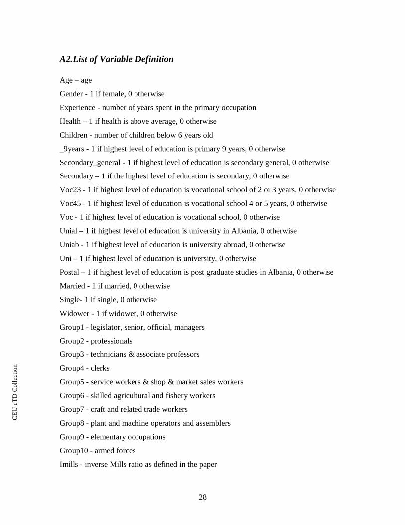
A2.List of Variable Definition

Age – age

Gender - 1 if female, 0 otherwise

Experience - number of years spent in the primary occupation

Health – 1 if health is above average, 0 otherwise

Children - number of children below 6 years old

_9years - 1 if highest level of education is primary 9 years, 0 otherwise

Secondary_general - 1 if highest level of education is secondary general, 0 otherwise

Secondary – 1 if the highest level of education is secondary, 0 otherwise

Voc23 - 1 if highest level of education is vocational school of 2 or 3 years, 0 otherwise

Voc45 - 1 if highest level of education is vocational school 4 or 5 years, 0 otherwise

Voc - 1 if highest level of education is vocational school, 0 otherwise

Unial – 1 if highest level of education is university in Albania, 0 otherwise

Uniab - 1 if highest level of education is university abroad, 0 otherwise

Uni – 1 if highest level of education is university, 0 otherwise

Postal – 1 if highest level of education is post graduate studies in Albania, 0 otherwise

Married - 1 if married, 0 otherwise

Single- 1 if single, 0 otherwise

Widower - 1 if widower, 0 otherwise

Group1 - legislator, senior, official, managers

Group2 - professionals

Group3 - technicians & associate professors

Group4 - clerks

Group5 - service workers & shop & market sales workers

Group6 - skilled agricultural and fishery workers

Group7 - craft and related trade workers

Group8 - plant and machine operators and assemblers

Group9 - elementary occupations

Group10 - armed forces

Imills - inverse Mills ratio as defined in the paper

CE

UeT

DC

olle

ctio

n

29

A3. TABLES

Table A3.1. Summary Statistics of LSMS 2002-2005

Table A3.2. Summary Statistics for 2002-2005 data used in OLS Regressions2002 2003 2004 2005

Observations Females 684 345 160 1468Males 1369 673 1100 2482Total 2053 1018 1260 3950

Average Age Females 46.7 37.6 40.1 43.9Males 46.2 40.6 44.8 47.4

Average Monthly Wage Females 21586 15958 14392 21570 (in new Lek) Males 18586 21267 20874 22212Average Monthly Hours Females 160 43 155 178

Males 162 153 161 179Marital Status Married 1780 888 1092 3399

Divorced 70 44 40 27Widower 90 41 54 174Single 90 42 64 338other 23 3 5 12

Major Occupation Group7: 408 Group7:239 Group7:333 Group6:968Group2: 389 Group2:205 Group6:315 Group7:720Group3: 198 Group8:127 Group5:139 Group2:520

Year Total Observations Working

2002 Females 8126 2636 31%Males 8395 2807 34%Total 16521 5443 33%

2003 Females 3929 1420 35%Males 4044 1326 33%Total 7973 2746 34%

2004 Females 4064 1215 30%Males 3961 1676 41%Total 8025 2891 36%

2005 Females 8586 2348 26%Males 8712 3359 39%Total 17298 5707 33%

CE

UeT

DC

olle

ctio

n

30

Table A3.3. Summary Statistics for 2003-2004

2003 2004

MeanStandardDeviation Mean

StandardDeviation

AGE 31.10548 2301.751 32.43252 21.47689WAGE 19415.72 12911.01 18324.62 22465.63GENDER 0.492788 0.49999 0.506417 0.49999MARRIED 0.478615 0.499979 0.465919 0.498868SINGLE 0.254986 0.499574 0.229283 0.420398WIDOWER 0.047912 0.43588 0.049221 0.216343

DIVORCED 0.005393 0.213593 0.003988 0.063025HEALTH 0.915841 0.073245 0.905256 0.292888_9YEARS 0.033112 0.277644 0.278006 0.448044SECONDARY_GENERAL 0.051047 0.17894 0.279502 0.448782VOC23 0.037627 0.220108 0.07053 0.256053VOC45 0.267152 0.190304 0.039626 0.195091UNIAL 0.037627 0.4425 0.010592 0.102377UNIAB 0.025586 0.190304 0.003988 0.063025POSTAL 0.031983 0.157908 0.002243 0.04731NONE 0.272294 0.175966 0.000498 0.022322WORKED 0.344663 0.445168 0.360623 0.480211HOURS 29.46244 2.033511 60.92162 85.57973GROUP1 0.006397 69.09495 0.009221 0.095589GROUP2 0.027342 0.079727 0.028162 0.165446GROUP3 0.015302 0.163089 0.017695 0.131848GROUP4 0.004264 0.122757 0.009969 0.099351GROUP5 0.029976 0.065167 0.034393 0.182247GROUP6 0.176094 0.170532 0.182679 0.386427GROUP7 0.036122 0.380924 0.052835 0.223718GROUP8 0.021071 0.186605 0.022181 0.14728GROUP9 0.026213 0.14363 0.00972 0.098114EXPERIENCE 8.875318 0.15978 7.211978 6.172775CHILDREN 0.703123 0.970739 0.638131 0.980819

CE

UeT

DC

olle

ctio

n

31

Table A3.4. OLS Regression ResultsDependent Variable: LOG(HOURS)2002 2003 2004 2005 POOLED

Independent Variable Coefficient Coefficient Coefficient Coefficient Coefficient

C 3.985128* 4.565998* 3.819058* 4.440375* 4.268822*AGE -0.0006 -0.00419** 0.007448* -0.00067 0.000317GENDER -0.01412 -0.10387*** -0.01334 -0.00495 -0.01034MARRIED -0.10738* -0.06228 0.027383 0.088419 -0.02153SINGLE -0.04868 -0.18063 -0.04082 0.071454 -0.02388WIDOWER -0.13942* -0.02734 0.017422 0.179423** 0.005692LOG(PAYMENT) 0.116597* 0.076007** 0.087851* 0.066092* 0.074405*YEAR2003 0.068141*YEAR2004 0.035128***YEAR2005 0.157424*

R-squared 0.016647 0.023051 0.054487 0.031278 0.041136Adjusted R-squared 0.013763 0.014494 0.049959 0.029791 0.040045S.E. of regression 0.533057 0.465251 0.476828 0.40925 0.46132Sum squared resid 581.3713 148.2743 284.8877 654.702 1683.588Log likelihood -1617.98 -448.885 -851.196 -2054.4 -5106.22

* significant at 1% ** significant at 5% *** significant at 10%

CE

UeT

DC

olle

ctio

n

32

Table A3.5. OLS Results for 2003-2004

* statistically significant at 1% ** statistically significant at 5% statistically significant at 10%standard errors are given in the brackets

Dependent variable: log(H)2003 2004

Independent Variable Coefficient Coefficient

C3.835905*(0.539478)

4.201786*(0.137524)

AGE0.022684

(0.018268)0.027893*(0.004874)

AGE^2-0.000302(0.000221)

-0.000337*(5.57E-05)

MARRIED-0.148638(0.155656)

-0.1159*(0.042975)

SINGLE-0.034271(0.159005)

-0.09717**(0.048525)

WIDOWER-0.286706(0.245173)

-0.157974**(0.077281)

_9YEARS-0.071029(0.147403)

-0.125485**(0.065151)

SECONDARY_GENERAL-0.056027(0.115403)

-0.119687**(0.065442)

VOC23-0.041146(0.116453)

-0.085138(0.06907)

VOC450.006536

(0.114492)-0.056135(0.074102)

UNIAL-0.062312(0.038289)

-0.009758(0.083184)

UNIAB0.096475

(0.117559)-0.026749(0.123896)

POSTAL0.11349

(0.082037)

GENDER-0.097265(0.056589)

-0.107448*(0.01884)

CHILDREN-0.009113(0.018098)

-0.007328(0.006571)

HEALTH0.207557

(0.138181)0.079406

(0.051178)

LOG(WAGE)0.080339**(0.245173)

0.067213*(0.008508)

R-squared 0.042847 0.135551Adjusted R-squared 0.019921 0.128473S.E. of regression 0.465860 0.335468Sum squared resid 144.9733 233.6303

Log likelihood -440.1153 -675.0907

CE

UeT

DC

olle

ctio

n

33

REFERENCES

Albanian Institute of Statistics. (2002) 1993-2001 Statistical Yearbook. INSTAT Albania.

Albanian Institute of Statistics. (2004) Albania in figures 2004. INSTAT Albania.

Albania LSMS 2002, LSMS 2003, LSMS 2004, LSMS 2005. (2008) World Bank (WB)[Internet]. Available from: http://www.worldbank.org/ [Accessed 30 May 2008].

Bosworth, D., Dawkins, P. & Stromback, T. (1996) The economics of the labor market.Addison Wesley Longman, pp 67.

Carletto, G. B., Stampini, D. & Stampini, M. (2005) Familiar faces, familiar places: Therole of family networks and previous experience for Albanian migrants. ESA WorkingPaper. NO. 05-03.

EIU Albania Country Profile, 2004 In: International Labour Office and Council ofEurope. (2006) Employment Policy Review, Albania. Strasbourg , Council of Europe.

El-Hamidi, F. (2003) Poverty and labor supply of women: evidence from Egypt. In:TenthAnnual Conference of the Economic Research Forum (ERF), University of Pittsburgh.October.

Employment Policy Review, Albania, International Labor Organization, prepared byInternational Labor Office and the Council of Europe , 2003-2004

Heckman J. J. (1980) Sample selection bias as a specification error with an application tothe estimation of labor supply functions. in James P. Smith, ed., Female Labor Supply:Theory and Estimation, Princeton University Press, 1980, pp. 206-248.

International Labour Office and Council of Europe. (2006) Employment Policy Review,Albania. Strasbourg , Council of Europe.

Killingsworth, M.R. (1983) Labor Supply. Cambridge University Press.

Lokshin, M. (2004) Household childcare: choices and women’s work behavior in Russia.Journal of Human Resources, Vol. 39(4): pp.1094-1115.

Muço, M., Sanfey, P., Luci, E. & Hashorva, G. (2004) Private sector and labor marketdevelopments in Albania: Formal versus Informal. Global Development NetworkSoutheast Europe. April .

Robins, L. (1930) On the elasticity of demand for income in terms of effort. Economica(29), pp.123-129.