estimating fixing effort and schedule ... - moodle.fct.unl.pt

SOFTWARE PROCESS IMPROVEMENT AND PRACTICESoftw. Process Improve. Pract. 2008; 13: 35–50

Published online in Wiley InterScience(www.interscience.wiley.com) DOI: 10.1002/spip.366

Estimating Fixing Effortand Schedule based onDefect InjectionDistribution

Research SectionQing Wang1*, Lang Gou1,2, Nan Jiang1,2, Meiru Che1,2,Ronghui Zhang1,2, Yun Yang3 and Mingshu Li1

1 Institute of Software, Chinese Academy of Sciences, Beijing, China2 Graduate University of Chinese Academy of Sciences, Beijing, China3 CITR, Swinburne University of Technology, Melbourne, Australia

Detecting and fixing defects are key activities in a testing process, which consume two kinds ofskill sets. Unfortunately, many current leading software estimation methods, such as COCOMOII, mainly estimate the effort depending on the size of software, and allocate testing effort propor-tionally among various activities. Both efforts on detecting and fixing defects, are simply countedinto software testing process/phase and cannot be estimated and managed satisfactorily. In fact,the activities for detecting defects and fixing them are quite different and need differently skilledpeople. The inadequate effort estimation leads to the difficulty of test process management. It isalso the main problem which causes software project delays. In this article, we propose a methodon Quantitatively Managing Testing (TestQM) process including identifying performance objec-tives, establishing a performance baseline, establish a process-performance model for fixingeffort, and establishing a process-performance model for fixing the schedule, which supportshigh-level process management mentioned in Capability Maturity Model Integration (CMMI).In our method, defect injection distribution (DID) is used to derive estimation of fixing effort andschedule. The TestQM method has been successfully applied to a software organization for theirquantitative management of testing process and proved to be helpful in estimating and control-ling defects, effort and schedule of the testing process. Copyright 2008 John Wiley & Sons, Ltd.

KEY WORDS: software measurement; quantitative process management; testing process; process-performance baseline; process-performance model

1. INTRODUCTION

Quantitative management is among the advancedfeatures of highly mature processes as defined in

∗ Correspondence to: Qing Wang, Laboratory for Internet Soft-ware Technologies, Institute of Software, The Chinese Academyof Sciences, No. 4 South Fourth Street, Zhong Guan Cun, Beijing100080, China†E-mail: [email protected]

Copyright 2008 John Wiley & Sons, Ltd.

CMMI (Chrissis et al. 2006), which provides insightto the degree of goal fulfillment and root causes ofsignificant process/product deviation.

Testing is an important method for quality con-trol. There are substantial research on testing tech-niques and testing management method (Maximi-lien and Williams 2003, Gould et al. 2004, Clarke andRosenblum 2006, Bertolino 2007). Testing is also animportant process that needs to be managed quanti-tatively for high-maturity organizations. However,

Research Section Q. Wang et al.

quantitative management method of the testing pro-cess is complex because it is constrained not only bythe size of product, but also by the quality of prioractivities in the lifecycle, such as design and coding.The more defects injected in the earlier activities, themore effort is needed to fix and verify them. Howto estimate the effort and the defects-related data,establish a process-performance baseline (P-BL) anda process-performance model of testing process arethe challenges. In fact, many software projects aredelayed due to the slippage of the testing activities.

Many estimation methods estimate or predictthe effort and defect separately. For example,COCOMO II (Boehm et al. 2000) is a famouscost estimation method with a family of exten-sion models with respect to different types ofdevelopment needs. COnstructive QUALity MOdel(COQUALMO) (Boehm et al. 2000) is one of thesemodels which can be used to estimate the qualityof software products in terms of defect density. Butit does not consider the interrelationship betweendefect and effort. The testing effort comes mainlyfrom the general percentage of the total estimatedeffort, which does not benefit high-level processmanagement in CMMI.

As we know, even though there are many veri-fication activities during the software developmentcycle, testing is still the most common and impor-tant method to detect and fix defects. The defectsdetected in testing are injected not only from coding,but also from requirements analysis and softwaredesign. In this article, we propose a method onQuantitatively Managing Testing (TestQM) process.Based on the TestQM method, the performanceobjectives of testing process are identified. Thensome statistical techniques are used to analyze thedata related to these objectives and some process-performance model are established. The TestQMmethod has been successfully applied to a softwareorganization and appears to be very useful in help-ing software organizations quantitatively managetesting process.

The Institute of Software, Chinese Academy ofSciences (ISCAS) is a research and developmentorganization in China. ISCAS developed a toolkitcalled SoftPM (Wang and Li 2005) which is used tomanage software projects and has been deployedto many software organizations in China. The dataused in this article comes from 17 projects based onfacilitating SoftPM.

This article is organized as follows. The TestQMmethod is presented in Section 2. Section 3 intro-duces the empirical study on establishing quantita-tive management model for testing process basedon the TestQM method. Section 4 describes the prac-tice of quantitatively managing the testing processby using the model established in Section 3. Relatedwork is discussed in Section 5. Section 6 summa-rizes our conclusions and points out future work.

2. THE METHODOLOGY

This section presents the TestQM method of quan-titatively managing the testing process, which sup-ports high-level process management mentionedin CMMI. As shown in Figure 1, the four steps ofthe TestQM method are to: (i) identify the perfor-mance objectives (P-Objs) to be managed quanti-tatively and construct data samples; (ii) establishthe P-BL for the identified P-Objs; (iii) establishthe process-performance model for fixing effort;and (iv) establish the process-performance modelfor fixing schedule.

As shown in Figure 1, by using the methodology,the empirically based models for the testing processcan be established based on the analysis of historicaldata, which will be described in Section 3. Softwareprojects can use the model to estimate and controlthe defects, effort and schedule quantitatively,which will be described in Section 4.

2.1. Identify P-Objs and Construct Data Samples

Normally, the effort of detecting and fixing defects,and the defect-injected phase are sensitive data thatwe should consider for testing process. A generalassumption is that the effort of detecting and fixingdefects should consume a certain percentage in thetotal development effort, and the effort of fixingdefects is influenced by the defect number and thedefect-injected phase. In the TestQM method, fourP-Objs have been identified as follows:

1. Percentage of Detecting Effort (%EffDetect):Detecting effort means the effort for all detect-ing activities including test planning, test casepreparation, test implementation and fix verifi-cation. The percentage of the detecting effort inthe total effort is %EffDetect.

2. Defect Injection Distribution (DID): In general,many software organizations collect defect

Copyright 2008 John Wiley & Sons, Ltd. Softw. Process Improve. Pract., 2008; 13: 35–50

36 DOI: 10.1002/spip

Research Section Estimating Fixing Effort and Schedule

Defectinjection

distribution

Process-performance

model forfixing effort

Process-performance

model forfixing

schedule

Initial estimation

Tracking

Re-estimation

Size, Total effort

Estimated defects injectiondistributionEstimated detecting effortEstimated fixing effort

Actual defects injection distribution

Re-estimated fixing effortRe-estimated fixing schedule

ApplicationEmpirically-based Models

Steps 1: Identify P-Objs andconstruct data samples

Step 2: Establish P-BL ofidentified P-Objs

Step 3: Establish process-performance model for fixing

effort

Step 4: Establish process-performance model for fixing

schedule

Methodology

Causal analysis

Model refinement

Refined models

1

2

3

1

2

Figure 1. The illustration of the TestQM method

data for quality control. There are alwayssome defects injected in the early phases,which are only detected during the testingactivities, even in high-maturity organizations.In our method, three primary phases, namelyrequirements, design and coding, are used toclassify the corresponding injected phases foreach defect. The corresponding percentages ofdefects injected in these phases are denoted as:requirements, (%DIReq); design, (%DIDesign); andcoding, (%DICode) respectively.

The principles of assigning the injected phase aredescribed as: (i) defect injected in the requirementsphase: a defect that is due to poor requirements,such as inconsistent and unclear requirements;(ii)a defect injected in the design phase: a defectthat is due to poor design, such as unclear inter-face, misunderstanding of requirements and incom-plete data verification; and (iii) a defect injectedin the coding phase: a defect that is due topoor coding, such as incorrect words in a Webpage and inconsistent code against requirements ordesign.3. Schedule Factor for Defect Fixing (SFFix). For

each defect, the opening date is the day thedefect is being submitted, and the closing dateis the day the defect is being confirmed as

repaired. The schedule of defect fixing (ScedFix)can be calculated by the formula below.

ScedFix = closing date − opening date + 1.

Sometimes, certain defects are assigned ‘deferred’and not to be fixed in the current release due tobusiness pressures. In this case, we take the day thedefect is being deferred and calculate the ScedFix asshown below.

ScedFix = deferred date − opening date + 1.

The ScedFix for deferred defects means the sched-ule of the defect being dealt with.

For each project, the average schedule of fixingone defect (AScedFix) injected in each phase can becalculated by the formula below.

AScedFix of each phase = total ScedFix/ total defects

injected in the phase

Normally, the AScedFix of coding phase(AScedCode) is the shortest. We use the AScedCode

as the benchmark (i.e. SFCode), and calculate theratio of AScedFix of requirements phase (AScedReq)to AScedCode, as well as the ratio of AScedFix of


DOI: 10.1002/spip 37


design phase (AScedDesign) to AScedCode by the for-mula below.

SFCode = 1

SFReq = AScedReq/AScedCode

SFDesign = AScedDesign/AScedCode

4. Percentage of Fixing Effort (%EffFix): Fixingeffort data means the effort for all defect-fixingactivities including defect analysis and fixing.%EffFix is the percentage of the fixing effort inthe total effort.

2.2. Establish P-BL of Identified P-Objs

P-BL is the basis for quantitative process manage-ment. As defined in CMMI, P-BL is a documentedcharacterization of the actual results achieved byfollowing a process, which is used as a benchmarkfor comparing actual process performance againstexpected process performance (Chrissis et al. 2006).P-BL is established based on the statistical analysisof historical data. There are many methods and tech-niques, such as Baseline-Statistic-Refinement (BSR)(Wang et al. 2006) and Statistical Process Control(SPC) (Florac and Careton 1999, Jalote and Saxena2002) which can be used to establish P-BL.

Defect fixing is an important activity of softwaredevelopment, which demands a certain amountof effort. In the International Software BenchmarkStandard Group (ISBSG), (www.isbsg.org), thefixing effort is collected and counted in reworkeffort. However, many effort estimation methodsdo not pay sufficient attention to the effort of defectfixing; instead, they just include it in the testingactivities. Normally, defect detecting is performedby a testing team, and defect fixing is performedby a development team. Estimating their effortseparately is helpful for an organization to planits human resources and schedules. In addition, thefixing effort is strongly correlated with the numberand injected phase of defects. Splitting them andestablishing their P-BLs are very useful to managetesting process quantitatively.

For high-maturity software organizations, thedefect-related process performance, such as defectinjection, defect removal, and defect density, alsohas some common and stable properties. Manymethods discuss the defect removal ratio anddefect density. These are very useful and easy to

understand. Here we focus on the defect injectionand the correlation between the defects and effortneeded to fix them.

2.3. Establishing A Process-Performance Modelfor Fixing Effort

In CMMI, the process-performance model is adescription of the relationships among attributesof a process and its work products that are devel-oped from historical process-performance data, andcalibrated using collected process and productmeasures from the project, and are used to pre-dict results to be achieved by following a process(Chrissis et al. 2006).

In the testing activities, there is a consensus thatthe earlier a defect is injected, the more effort isneeded to fix it. In contrast, the later a defect isinjected, the less effort is needed to fix it. So, defectsinjected in an earlier phase, such as the requirementsphase, have the effect of increasing the defect-fixingeffort, whereas, defects injected in a later phase, suchas the coding phase, have the effect of decreasingthe defect-fixing effort.

After constructing defect-related data samples,software organizations can discover some moreprecise correlation between defects and fixingeffort. The process-performance model for fixingeffort is based on this hypothesis. There are somestatistical methods which can be used to analyzethe correlation between DID and %EffFix, such asmultiple regression analysis (Wooldridge 2002).After the correlation between DID and %EffFix hasbeen analyzed, the regression equation betweenDID and %EffFix can be used to refine the estimationof fixing effort after testing. The outcome canprovide a guideline to estimate the effort of defectfixing based on the defects and the distribution ofinjection phases. So, after testing, project managerscould reestimate and replan their fixing efforteffectively. The factors of regression equation couldbe refined and calibrated based on the historicaldata of software organizations. Thereafter, it can bebetter applied in these organizations.

2.4. Establishing A Process-Performance Modelfor Fixing Schedule

As we mentioned before, many software projects aredelayed due to the slippage of the testing process. Infact, many testing processes are delayed due to the


38 DOI: 10.1002/spip


schedule overrun of defect-fixing activity. To solvethis problem, TestQM uses a more effective methodon estimating schedule of defect-fixing activity.

An algorithm to help estimate the schedule ofdefect-fixing activity is established based on theanalysis of SFFix and the effort of defect fixing. Thealgorithm applies the following principles:

• Shortest schedule. Based on the total effort ofdefect fixing, the defect-fixing schedule shouldbe as short as possible.

• Concurrent defect fixing. Defects which requirea long fixing schedule should be fixed concur-rently if there are sufficient human resourcesavailable.

The basic ideas of the algorithm are: (i) the fixingschedule of defects injected in requirements shouldbe allocated first since the AScedReq is the longest,which is the basis of the fixing schedules of defectsinjected in design and coding; (ii) if the number ofdefects injected in the design and the number ofdefects injected in the coding are similar, as well asif the SFReq is longer than the sum of SFDesign andSFCode, then the fixing schedule of defects injectedin design and coding could be allocated serially.Especially, in the algorithm, we assume that if 1/2< numbers of defects injected in design/numbersof defects injected in coding <2, it means that thenumbers of defects injected in design and coding aresimilar; and (iii) in the other cases, the schedule ofdefects injected in design and the schedule of defectsinjected in coding should be allocated concurrently.

The definitions used in the algorithm and thedescription of the algorithm are shown as follows:

• Assume the defects detected in testing processis {di}, i = 1 . . . n, n is the total number of defectsdetected in the testing process. Especially, {dr},{dd}, {dc} denote the defects injected in require-ments, design and coding phases respectively.

• Assume the numbers of defects injected inrequirements, design and coding phases are Dr,Dd, Dc respectively.

• Assume ∀i ∈ [1, n], si is the fixing schedule for di.• Assume e is the effort of one day for a every

full-time staff

Algorithm 1: Allocate the ScedFix.Input: effort of defect fixing (E)

AScedReq, AScedDesign, AScedCode

SFReq, SFDesign, SFCode

Output: ScedFix (S = {<d1, s1 >, <d2, s2 > · · · <

dn, sn >})Steps: S = �

1. If Dr > 0Then allocate si for each dr as concurrently as

possible.

S = S+ < d1, s1 > + < d2, s2 > + · · ·+ < dn, sn >

di ∈ dr i = 1 · · · Dr

Assume Sr is the schedule for fixing all dr

2. Else If 1/2 < Dd/Dc < 2 and SFReq >= SFDesign

+ SFCode

Then M = int (SFReq/(SFDesign + SFCode))

Assign no more than M × (dd + dc) to be fixedserially.

S = S+ < d1, s1 > + < d2, s2 > + · · ·+ < dn, sn >

di ∈ dd + dc i = 1 . . . Dd + Dc

3. Else allocate the schedule for {dd} and {dc}concurrently.

N = int (Sr/AScedDesign)

Assign no more than N × dd to be fixed serially.

S = S+ < d1, s1 > + < d2, s2 > + · · ·+ < dn, sn >

di ∈ {dd} i = 1 . . . Dd

N′ = int (Sr/AScedCode)

Assign no more than N′ × dc to be fixed serially.

S = S+ < d1, s1 > + < d2, s2 > + · · ·+ < dn, sn >

di ∈ {dc} i = 1 . . . Dc

4. If E >n∑

i=1(si × e) Then go to Step 1.

The P-BL of SFFix and the Algorithm 1 compose theprocess-performance model for fixing schedules.

Up to now, the P-BLs of the identified P-Objs, thecorrelations between the P-Objs, and the algorithmof estimating defect-fixing schedules compose thequantitative management model for the testingprocess. In the model, the P-BLs of %EffDetect, DIDand %EffFix, and the correlations between DIDand %EffFix are used for quantitatively controllingdefects and effort of the testing process, while theP-BL of SFFix and the algorithm is used for managingthe schedule of defect-fixing activities.


DOI: 10.1002/spip 39


Table 1. Brief information about the 16 Web-based system development projects

Projects Number ofstaff

Schedule(Months)

Size(KLOC)

Applicationdomain

Processperformance

1 12 12 151.9 Application system integration2 15 7 173.1 E-government3 5 6 18.2 E-government4 14 7.5 311.2 Application system integration5 6 4 76.9 Website design and development Successful projects with little6 3 3 45.9 Website design and development schedule overruns.7 6 2 17.0 Information management8 14 9 280.4 E-government9 4 5.5 45.0 E-government All performed requirements,10 12 7 55.5 Information management design, coding and testing11 9 5 60.7 E-government processes12 4 2 19.6 Information management13 11 9 90.4 Application system integration14 12 4.5 250.5 Application system integration15 5 6 80.0 Information management16 4 7 30.0 E-government

3. EMPIRICALLY BASED MODELS

This section presents some empirical results onestablishing a quantitative management model forthe testing process by using the TestQM methodpresented in Section 2. We collected testing processdata from 16 Web-based system developmentprojects, and decided upon the empirically basedmodels for testing process. Web-based developmenttechniques have been widely applied in China.These 16 projects came from two closely relatedsoftware organization entities. The two entities havethe self-governed process management system andwere rated at CMMI maturity level 3 and movingtowards CMMI maturity level 4 during the periodof our data collection.

Table 1 summarizes the brief information aboutthe 16 projects. We collected the DID, %EffDetect,%EffFix and SFFix data from the 16 projects indicatedearlier. These data were reported by engineers andwere collected in SoftPM (Wang and Li 2005).

3.1. Defect Injection Distribution

For the 16 projects, all the defects considered weredetected in the testing activities. These defects wereclassified into four categories: critical defects, seri-ous defects, noncritical defects and cosmetic defects.In this article, we only describe the total defects col-lected without distinguishing them. Table 2 showsthe defects injected in three primary phases and theDIDs of the 16 projects.

The XmR (individuals and moving range) controlchart (Grant and Leavenworth 1996, Florac andCareton 1999) is applied to analyze the DID data.Assume that the sequence of data sample is Xi, themoving range (mR) is:

mRi = |Xi − Xi−1| i = 2 . . . n

According to the theory of statistics, we can getthe upper control limit (UCL), central line (CL), andlower control limit (LCL) for mR-chart and X-chartas follows:

UCLmR = 3.268mR, CLmR = mR, LCLmR = 0

UCLx = X + 2.660mR, CLx = X,

LCLx = X − 2.660mR

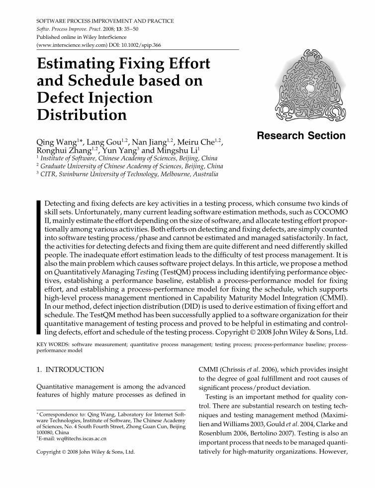
Tables 3–5 show the XmR chart control limits.Figures 2–4 show the XmR control charts for%DIReq, %DIDesign and %DICode respectively.

For the three XmR charts in Figures 2–4, all datapoints are distributed between the UCL and the LCLin both mR-chart and X-chart. Hence, the %DIReq,%DIDesign and %DICode were converged and the dis-tribution of defect injection appears to be stable.Therefore, the 14.9, 28.0 and 57.1% can be acceptedas the P-BLs of %DIReq, %DIDesign and %DICode, respec-tively, to be used to estimate the distribution ofdefect injection.


40 DOI: 10.1002/spip


Table 2. Defects injected in each phase and the DIDs of the 16 projects

Projects Numberof defects injected in

requirements

%DIReq Number ofdefects injected in

design

%DIDesign Number of defectsinjected in

coding

%DICode

1 19 10.1 41 21.8 128 68.12 118 15.6 153 20.3 483 64.13 33 17.8 61 33.0 91 49.24 251 18.7 412 30.6 682 50.75 27 20.5 44 33.3 61 46.26 17 13.3 35 27.3 76 59.47 15 15.6 28 29.2 53 55.28 135 14.1 322 33.6 501 52.39 32 12.2 82 31.2 149 56.710 15 13.9 29 26.9 64 59.311 92 18.3 116 23.1 295 58.612 12 14.0 26 30.2 48 55.813 18 11.8 36 23.5 99 64.714 53 11.0 142 29.5 286 59.515 78 17.6 114 25.7 251 56.716 20 13.9 42 29.2 82 56.9

Table 3. XmR chart control limits for %DIReq data

UCLmR CLmR LCLmR UCLx CLx LCLx

10.2% 3.1% 0 23.2% 14.9% 6.6%

Table 4. XmR chart control limits for %DIDesign data


15.1% 4.6% 0 40.3% 28.0% 15.8%

Table 5. XmR chart control limits for %DICode data


15.9% 4.9% 0 70.0% 57.1% 44.2%

3.2. Process-Performance Model for Fixing Effort

We collected the total effort (in labor hour), defect-detecting effort (in labor hour) and defect-fixingeffort (in labor hour) of the 16 projects. Unfor-tunately, the detecting effort and fixing effort forindividual defects were not recorded. Hence wecould only collect the total detecting effort and totalfixing effort for the 16 projects. Then, we calcu-lated %EffDetect and %EffFix of the 16 projects. Table 6shows the total effort, detecting effort, fixing effort,%EffDetect and %EffFix of the 16 projects.

First, we analyze the %EffDetect data. The XmRchart control limits for %EffDetect data are shown in

Figure 2. XmR chart for %DIReq data of the 16 projects

Figure 3. XmR chart for %DIDesign data of the 16 projects

Table 7. We construct the XmR chart in Figure 5by using the %EffDetect data in Table 6 and controllimits in Table 7. For both the mR-chart and X-chart, all data points distributed between the UCLand the LCL. The process appears to be stable.The CLx (22.9%) can be considered as the P-BLof %EffDetect to be used to estimate defect-detectingeffort.


DOI: 10.1002/spip 41


Figure 4. XmR chart for %DICode data of the 16 projects

Table 6. Total effort, detecting effort, fixing effort, %EffDetect and%EffFix of the 16 projects

Projects Totaleffort

Detectingeffort

Fixingeffort

%EffDetect %EffFix

1 7,048 1,396 762 19.8 10.82 11,614 3,734 2,370 32.2 20.43 3,143 785 632 25.0 20.14 11,177 3,624 2,839 32.4 25.45 2,926 609 536 20.8 18.36 1,313 182 108 13.9 8.27 1,560 354 245 22.7 15.78 10,865 2,566 1,521 23.6 14.09 3,397 693 420 20.4 12.410 7,114 1,070 1,403 15.0 19.711 6,864 1,684 1,325 24.5 19.312 1,205 265 185 22.0 15.413 14,683 2,684 2,214 18.3 15.114 6,579 2,117 824 32.2 12.515 4,230 940 802 22.2 19.016 1,934 401 264 20.7 13.7

Table 7. XmR chart control limits for %EffDetect data


22.9% 7.0% 0 41.5% 22.9% 4.2%

Figure 5. XmR chart for %EffDetect data of the 16 projects

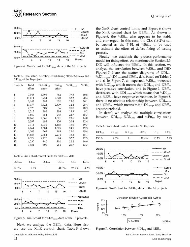
Next, we analyze the %EffFix data. Here also,we use the XmR control chart. Table 8 shows

the XmR chart control limits and Figure 6 showsthe XmR control chart for %EffFix. As shown inFigure 6, the %EffFix also appears to be stableand converged. In this case, the CLx (16.2%) canbe treated as the P-BL of %EffFix to be usedto estimate the effort of defect fixing of testingprocess.

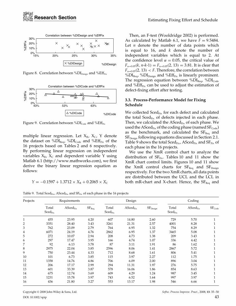
Finally, we establish the process-performancemodel for fixing effort. As mentioned in Section 2.3,DID will influence the %EffFix. In this section, weanalyze the correlation between %EffFix and DID.Figures 7–9 are the scatter diagrams of %DIReq,%DIDesign, %DICode and %EffFix data based on Tables 2and 6. In Figure 7, as expected, %EffFix increasedwith %DIReq, which means that %DIReq and %EffFix

have positive correlation; and in Figure 9, %EffFix

decreased with %DICode, which means that %DICode

and %EffFix have negative correlation. In Figure 8,there is no obvious relationship between %DIDesign

and %EffFix, which means that %DIDesign and %EffFix

are uncorrelated.In detail, we analyze the multiple correlations

between %DIReq, %DICode and %EffFix by using

Table 8. XmR chart control limits for %EffFix data


15.1% 4.6% 0 28.6% 16.2% 3.9%

Figure 6. XmR chart for %EffFix data of the 16 projects

Correlation between %DIReq and %EffFix

0%

10%

20%

30%

8% 12% 16% 20%

%DIReq

%E

ffFix

%DIReq

Figure 7. Correlation between %DIReq and %EffFix


42 DOI: 10.1002/spip


Correlation between %DIDesign and %EffFix

0%

10%

20%

30%

15% 20% 25% 30% 35%

%DIDesign

%E

ffFix

%DIDesign

Figure 8. Correlation between %DIDesign and %EffFix

Correlation between %DICode and %EffFix

0%

10%

20%

30%

43% 53% 63%

%DICode

%E

ffFix

%DICode

Figure 9. Correlation between %DICode and %EffFix

multiple linear regression. Let XR, XC, Y denotethe dataset on %DIReq, %DICode and %EffFix of the16 projects based on Tables 2 and 6 respectively.By performing linear regression on independentvariables XR, XC and dependent variable Y usingMatlab 6.1 (http://www.mathworks.com), we firstderive the binary linear regression equation asfollows:

Y = −0.1597 + 1.3712 × XR + 0.2065 × XC

Then, an F-test (Wooldridge 2002) is performed.As calculated by Matlab 6.1, we have F = 9.5484.Let n denote the number of data points whichis equal to 16, and k denote the number ofindependent variables which is equal to 2. Atthe confidence level α = 0.05, the critical value ofFα=0.05(k, n-k-1) = Fα=0.05(2, 13) = 3.81. It is clear thatFα=0.05(2, 13) < F. Therefore, the correlation between%DIReq, %DIDesign and %EffFix is linearly prominent.The regression equation between %DIReq, %DICode

and %EffFix can be used to adjust the estimation ofdefect-fixing effort after testing.

3.3. Process-Performance Model for FixingSchedule

We collected ScedFix for each defect and calculatedthe total ScedFix of defects injected in each phase.Then, we calculated the AScedFix of each phase. Weused the AScedFix of the coding phase (named SFCode)as the benchmark, and calculated the SFReq andSFDesign following equations discussed in Section 2.1.Table 9 shows the total ScedFix, AScedFix and SFFix ofeach phase in the 16 projects.

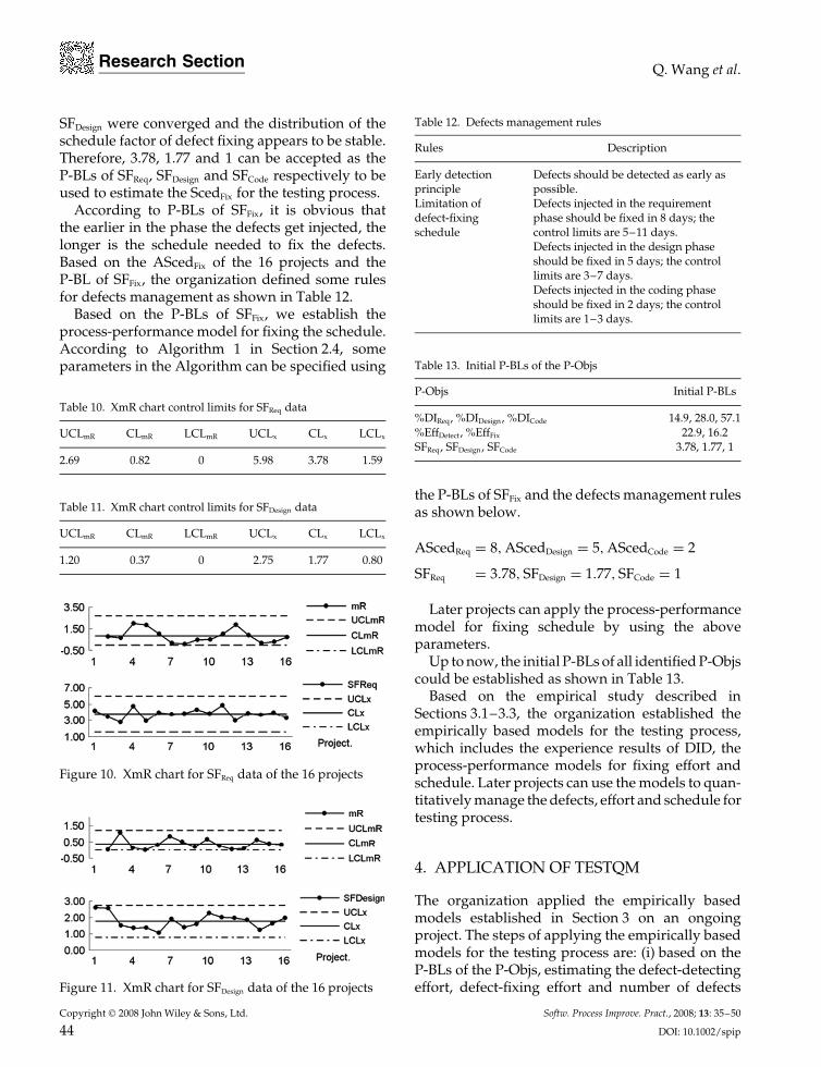
We use the XmR control chart to analyze thedistribution of SFFix. Tables 10 and 11 show theXmR chart control limits. Figures 10 and 11 showthe XmR control charts for SFReq and SFDesign

respectively. For the two XmR charts, all data pointsare distributed between the UCL and the LCL inboth mR-chart and X-chart. Hence, the SFReq and

Table 9. Total ScedFix, AScedFix and SFFix of each phase in the 16 projects

Projects Requirements Design Coding

TotalScedFix

AScedFix SFReq TotalScedFix

AScedFix SFDesign TotalScedFix

AScedFix SFCode

1 455 23.95 4.20 607 14.80 2.60 729 5.70 12 3351 28.40 3.43 3261 21.31 2.57 4001 8.28 13 762 23.09 2.79 764 6.95 1.32 754 8.29 14 6071 24.19 4.76 2862 6.95 1.37 3465 5.08 15 272 10.07 2.94 208 4.73 1.38 209 3.43 16 297 17.47 3.95 166 4.74 1.07 336 4.42 17 92 6.13 3.78 87 3.11 1.91 86 1.62 18 2975 22.04 3.85 2596 8.06 1.41 2867 5.72 19 750 23.44 4.33 712 8.68 1.61 806 5.41 110 101 6.73 3.85 115 3.97 2.27 112 1.75 111 1358 14.76 4.86 706 6.09 2.00 896 3.04 112 206 17.17 2.99 294 11.31 1.97 276 5.75 113 601 33.39 3.87 578 16.06 1.86 854 8.63 114 675 12.74 3.69 609 4.29 1.24 987 3.45 115 1231 15.78 3.97 743 6.52 1.64 997 3.97 116 436 21.80 3.27 553 13.17 1.98 546 6.66 1


DOI: 10.1002/spip 43


SFDesign were converged and the distribution of theschedule factor of defect fixing appears to be stable.Therefore, 3.78, 1.77 and 1 can be accepted as theP-BLs of SFReq, SFDesign and SFCode respectively to beused to estimate the ScedFix for the testing process.

According to P-BLs of SFFix, it is obvious thatthe earlier in the phase the defects get injected, thelonger is the schedule needed to fix the defects.Based on the AScedFix of the 16 projects and theP-BL of SFFix, the organization defined some rulesfor defects management as shown in Table 12.

Based on the P-BLs of SFFix, we establish theprocess-performance model for fixing the schedule.According to Algorithm 1 in Section 2.4, someparameters in the Algorithm can be specified using

Table 10. XmR chart control limits for SFReq data


2.69 0.82 0 5.98 3.78 1.59

Table 11. XmR chart control limits for SFDesign data


1.20 0.37 0 2.75 1.77 0.80

Figure 10. XmR chart for SFReq data of the 16 projects

Figure 11. XmR chart for SFDesign data of the 16 projects

Table 12. Defects management rules

Rules Description

Early detectionprinciple

Defects should be detected as early aspossible.

Limitation ofdefect-fixingschedule

Defects injected in the requirementphase should be fixed in 8 days; thecontrol limits are 5–11 days.Defects injected in the design phaseshould be fixed in 5 days; the controllimits are 3–7 days.Defects injected in the coding phaseshould be fixed in 2 days; the controllimits are 1–3 days.

Table 13. Initial P-BLs of the P-Objs

P-Objs Initial P-BLs

%DIReq, %DIDesign, %DICode 14.9, 28.0, 57.1%EffDetect, %EffFix 22.9, 16.2SFReq, SFDesign, SFCode 3.78, 1.77, 1

the P-BLs of SFFix and the defects management rulesas shown below.

AScedReq = 8, AScedDesign = 5, AScedCode = 2

SFReq = 3.78, SFDesign = 1.77, SFCode = 1

Later projects can apply the process-performancemodel for fixing schedule by using the aboveparameters.

Up to now, the initial P-BLs of all identified P-Objscould be established as shown in Table 13.

Based on the empirical study described inSections 3.1–3.3, the organization established theempirically based models for the testing process,which includes the experience results of DID, theprocess-performance models for fixing effort andschedule. Later projects can use the models to quan-titatively manage the defects, effort and schedule fortesting process.

4. APPLICATION OF TESTQM

The organization applied the empirically basedmodels established in Section 3 on an ongoingproject. The steps of applying the empirically basedmodels for the testing process are: (i) based on theP-BLs of the P-Objs, estimating the defect-detectingeffort, defect-fixing effort and number of defects


44 DOI: 10.1002/spip


Table 14. Extended P-BLs of Web-based system development projects

Detected defect density -DDD

Softwareproductivity - Prod

%DIReq, %DIDesign, %DICode %EffDetect, %EffFix SFReq, SFDesign, SFCode

4.01 Defects/KLOC 2.3 KLOC/Labor Month 14.9, 28.0, 57.1 22.9, 16.2 3.78, 1.77, 1

injected in each phase during the project planning;(ii) through the testing activities, collecting thedefect-related data and re-estimating the scheduleand effort of defect fixing when the actual P-Objshas abnormality; and (iii) after the testing process,refining the models if the testing process is normal.

4.1. Initial Estimation from P-BLs

As mentioned earlier, the organization was ratedat CMMI maturity level 3 and was moving toCMMI maturity level 4. It had some P-BLs inplace, such as detected defect density and softwareproductivity. The detected defect density refers to(defects/code size) where the defects are detected intesting activities (except unit testing). The indicatorof detected defect density is used to control thequality of software before being submitted fortesting. The software productivity is the meanproductivity (total size/total effort) which can beused to estimate the total effort. Besides these, weadded the process-performance model presented inSection 3 to optimize project management. The newextended P-BLs of Web-based system developmentprojects in the organization are shown in Table 14with some new quantitatively controlled objectivesdefined.

An ongoing Web-based system developmentproject, named TM, was selected in the organization.Table 15 summarizes the brief information about theproject.

Table 15. Brief information about project TM

No. of staff Plan schedule Plan size Development approach

8 4 months 67 KLOC Increment and Iteration

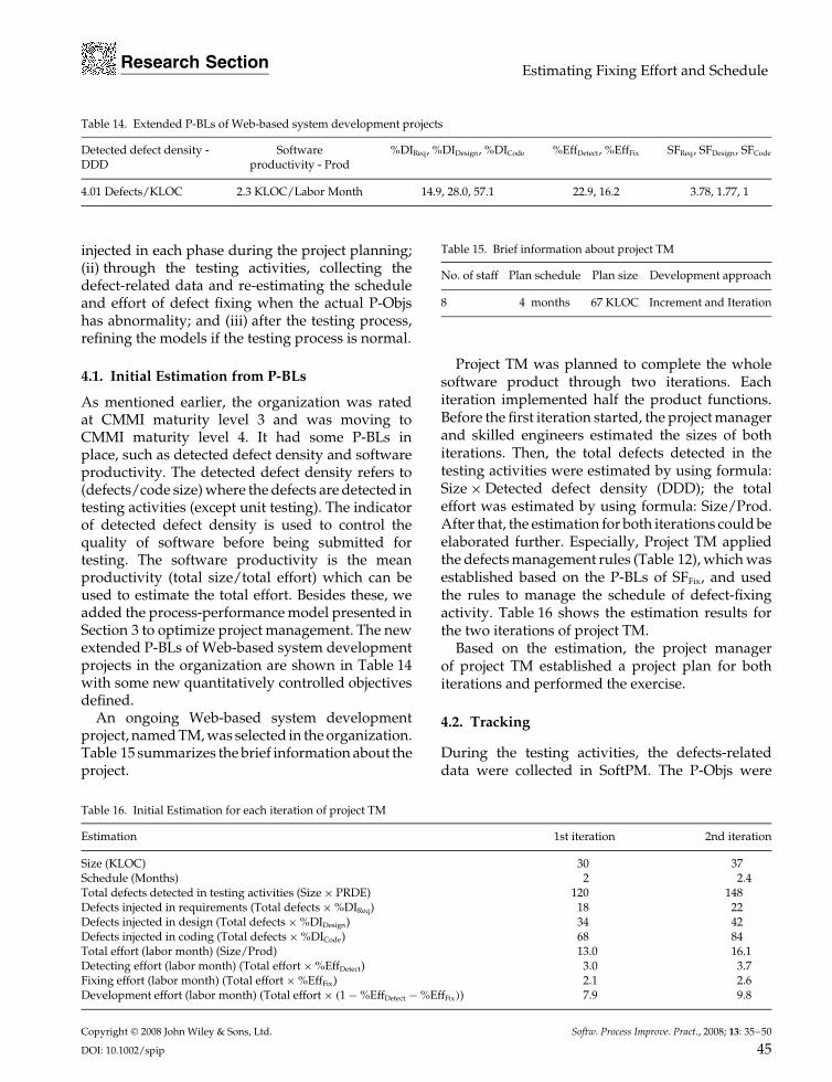
Project TM was planned to complete the wholesoftware product through two iterations. Eachiteration implemented half the product functions.Before the first iteration started, the project managerand skilled engineers estimated the sizes of bothiterations. Then, the total defects detected in thetesting activities were estimated by using formula:Size × Detected defect density (DDD); the totaleffort was estimated by using formula: Size/Prod.After that, the estimation for both iterations could beelaborated further. Especially, Project TM appliedthe defects management rules (Table 12), which wasestablished based on the P-BLs of SFFix, and usedthe rules to manage the schedule of defect-fixingactivity. Table 16 shows the estimation results forthe two iterations of project TM.

Based on the estimation, the project managerof project TM established a project plan for bothiterations and performed the exercise.

4.2. Tracking

During the testing activities, the defects-relateddata were collected in SoftPM. The P-Objs were

Table 16. Initial Estimation for each iteration of project TM

Estimation 1st iteration 2nd iteration

Size (KLOC) 30 37Schedule (Months) 2 2.4Total defects detected in testing activities (Size × PRDE) 120 148Defects injected in requirements (Total defects × %DIReq) 18 22Defects injected in design (Total defects × %DIDesign) 34 42Defects injected in coding (Total defects × %DICode) 68 84Total effort (labor month) (Size/Prod) 13.0 16.1Detecting effort (labor month) (Total effort × %EffDetect) 3.0 3.7Fixing effort (labor month) (Total effort × %EffFix) 2.1 2.6Development effort (labor month) (Total effort × (1 − %EffDetect − %EffFix)) 7.9 9.8


DOI: 10.1002/spip 45


Table 17. Actual performance data of the project TM

Actual performance data 1st iteration 2nd iteration

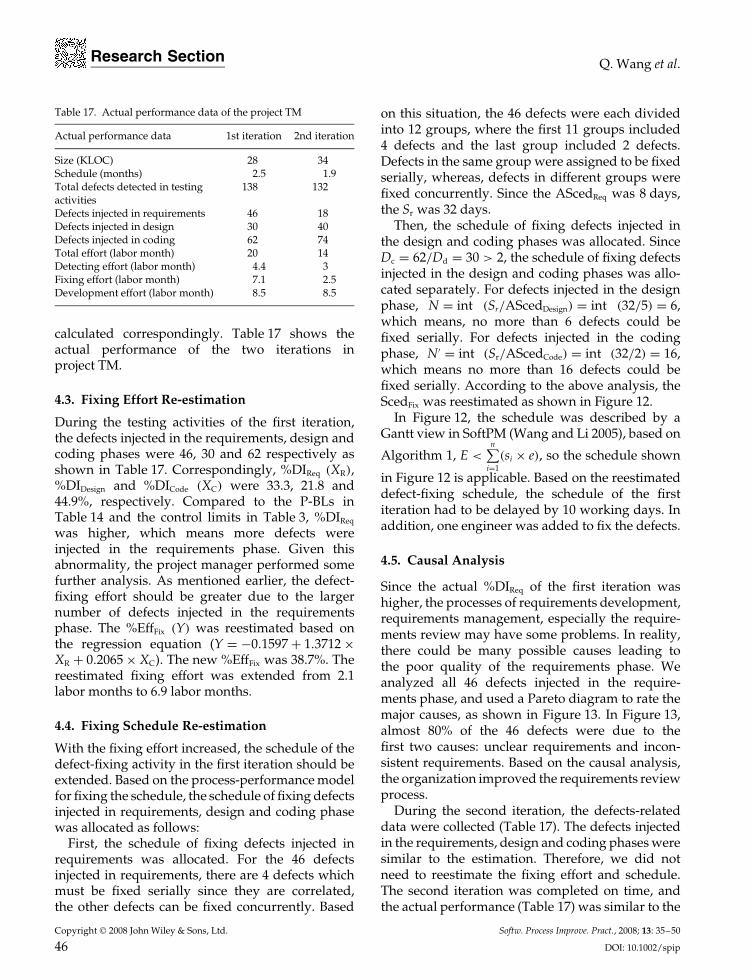
Size (KLOC) 28 34Schedule (months) 2.5 1.9Total defects detected in testingactivities

138 132

Defects injected in requirements 46 18Defects injected in design 30 40Defects injected in coding 62 74Total effort (labor month) 20 14Detecting effort (labor month) 4.4 3Fixing effort (labor month) 7.1 2.5Development effort (labor month) 8.5 8.5

calculated correspondingly. Table 17 shows theactual performance of the two iterations inproject TM.

4.3. Fixing Effort Re-estimation

During the testing activities of the first iteration,the defects injected in the requirements, design andcoding phases were 46, 30 and 62 respectively asshown in Table 17. Correspondingly, %DIReq (XR),%DIDesign and %DICode (XC) were 33.3, 21.8 and44.9%, respectively. Compared to the P-BLs inTable 14 and the control limits in Table 3, %DIReq

was higher, which means more defects wereinjected in the requirements phase. Given thisabnormality, the project manager performed somefurther analysis. As mentioned earlier, the defect-fixing effort should be greater due to the largernumber of defects injected in the requirementsphase. The %EffFix (Y) was reestimated based onthe regression equation (Y = −0.1597 + 1.3712 ×XR + 0.2065 × XC). The new %EffFix was 38.7%. Thereestimated fixing effort was extended from 2.1labor months to 6.9 labor months.

4.4. Fixing Schedule Re-estimation

With the fixing effort increased, the schedule of thedefect-fixing activity in the first iteration should beextended. Based on the process-performance modelfor fixing the schedule, the schedule of fixing defectsinjected in requirements, design and coding phasewas allocated as follows:

First, the schedule of fixing defects injected inrequirements was allocated. For the 46 defectsinjected in requirements, there are 4 defects whichmust be fixed serially since they are correlated,the other defects can be fixed concurrently. Based

on this situation, the 46 defects were each dividedinto 12 groups, where the first 11 groups included4 defects and the last group included 2 defects.Defects in the same group were assigned to be fixedserially, whereas, defects in different groups werefixed concurrently. Since the AScedReq was 8 days,the Sr was 32 days.

Then, the schedule of fixing defects injected inthe design and coding phases was allocated. SinceDc = 62/Dd = 30 > 2, the schedule of fixing defectsinjected in the design and coding phases was allo-cated separately. For defects injected in the designphase, N = int (Sr/AScedDesign) = int (32/5) = 6,which means, no more than 6 defects could befixed serially. For defects injected in the codingphase, N′ = int (Sr/AScedCode) = int (32/2) = 16,which means no more than 16 defects could befixed serially. According to the above analysis, theScedFix was reestimated as shown in Figure 12.

In Figure 12, the schedule was described by aGantt view in SoftPM (Wang and Li 2005), based on

Algorithm 1, E <n∑

i=1(si × e), so the schedule shown

in Figure 12 is applicable. Based on the reestimateddefect-fixing schedule, the schedule of the firstiteration had to be delayed by 10 working days. Inaddition, one engineer was added to fix the defects.

4.5. Causal Analysis

Since the actual %DIReq of the first iteration washigher, the processes of requirements development,requirements management, especially the require-ments review may have some problems. In reality,there could be many possible causes leading tothe poor quality of the requirements phase. Weanalyzed all 46 defects injected in the require-ments phase, and used a Pareto diagram to rate themajor causes, as shown in Figure 13. In Figure 13,almost 80% of the 46 defects were due to thefirst two causes: unclear requirements and incon-sistent requirements. Based on the causal analysis,the organization improved the requirements reviewprocess.

During the second iteration, the defects-relateddata were collected (Table 17). The defects injectedin the requirements, design and coding phases weresimilar to the estimation. Therefore, we did notneed to reestimate the fixing effort and schedule.The second iteration was completed on time, andthe actual performance (Table 17) was similar to the


46 DOI: 10.1002/spip


Figure 12. Reestimated defect-fixing schedule

Figure 13. Causal analysis of poor requirements

estimation (Table 16). Hence, the testing process ofthe second iteration is normal and stable.

4.6. Model Refinement

After project TM was finished, the organizationadded its data to the historical data and refined theempirically based models established in Section 3by using the data of the second iteration in projectTM, since the testing process in the second iterationof project TM was normal and stable.

Table 18 shows the actual performance data ofthe second iteration in project TM. Combined with

the performance data of the 16 projects (Tables 2, 6,and 9), we can refine the P-BLs of the P-Objs.

Similar to Section 3, we applied XmR controlcharts to analyze the distribution of %EffDetect, DID,SFFix and %EffFix data in the 17 projects. Due tospace limitation, we do not present the XmR controlcharts. As a result, in each XmR control chart, alldata points are distributed between the UCL andthe LCL in both mR-chart and X-chart. Hence,the %EffDetect, DID, SFFix and %EffFix data wereconverged and stable. Therefore, we can refine theP-BLs of %EffDetect, DID, SFFix and %EffFix as shownin Table 19.

Since the refined P-BLs were established basedon more data than the initial P-BLs (Table 13), the

Table 18. Actual performance data of the second iteration inproject TM

P-Objs Actual performance

%EffDetect 21.4%DIReq, %DIDesign, %DICode 13.6, 30.3, 56.1SFReq, SFDesign, SFCode 3.24, 1.80, 1%EffFix 17.9


DOI: 10.1002/spip 47


Table 19. Refined P-BLs of the P-Objs

P-Objs Refined P-BLs

%DIReq, %DIDesign, %DICode 14.8, 28.2, 57.0%EffDetect, %EffFix 22.8, 16.3SFReq, SFDesign, SFCode 3.75, 1.78, 1

refined P-BLs can quantitatively manage testingprocess more precisely. In the future, when theorganization has more project data of testingprocess, they can refine the P-BLs for %EffDetect,DID, SFFix and %EffFix continuously. Based on therefined P-BL of SFFix, the parameters of the process-performance model for fixing the schedule arerefined correspondingly.

We use the actual performance data of the seconditeration in project TM (Table 18) to refine thecorrelation regression between %DIReq, %DIDesign

and %EffFix as we described in Section 3.2.We analyze the multiple correlations between

%DIReq, %DICode and %EffFix by using multiple linearregression. Let XR, XC, Y denote the dataset on%DIReq, %DICode and %EffFix of the 17 projectsrespectively. By performing linear regression onthe independent variables XR, XC and the dependentvariable Y, we first derive the refined binary linearregression equation as follows:

Y = −0.1249 + 1.2910 × XR + 0.1700 × XC

Then, an F-test (Wooldridge 2002) is performed.As calculated by Matlab 6.1, we get the F statisticF = 8.8700. Let n denote the number of data pointswhich is equal to 17, and k denote the numberof independent variables which is equal to 2. Atthe confidence level α = 0.05, the critical value ofFα=0.05(k, n-k-1) = Fα=0.05(2, 14) = 3.74. It is clear thatFα=0.05(2, 14) < F. Therefore, the refined correlationbetween %DIReq, %DIDesign and %EffFix is linearlyprominent.

Up to now, the models established in Section 3have been refined. The experience from this casestudy validates that the TestQM method presentedin Section 2 and the models established in Section 3are helpful for improving quantitatively managingtesting process. And the TestQM method can beused in initial estimation, tracking the processperformance, identifying abnormality of process,analyzing the causes, reestimating the fixing effortand schedule, and improving the process to keep itcontrollable.

5. RELATED WORK

COnstructive COst MOdel (COCOMO) II (Boehmet al. 2000) is a widely used estimation model, whichallows one to estimate the total effort of a projectdepending on the estimated size. It provides twosets of empirical results on effort distribution forboth waterfall and RUP lifecycle phases, which canbe used to estimate effort of each phase includingtesting activities proportionally. COCOMO II can-not predict the effort of defect detecting and fixingaccurately. COQUALMO (Boehm et al. 2000) is aquality-model extension to COCOMO II. It is usedto estimate defects injected in different activities,and defects removed by defect removal activities.COQUALMO does not associate the defects withthe effort of defect fixing.

Software Productivity Research (SPR) (Jones2000) (http://www.spr.com) is a provider of con-sulting services to help companies manage softwaredevelopment processes. SPR collected data fromabout 9000 projects and reported the percentagesof the testing effort for system software, militarysoftware, commercial software, MIS and outsourc-ing software. Mizuno et al. (2002) develop a linearmultiple regression model of estimating the test-ing effort. In the model, the testing effort can beobtained from the design and review efforts, andare also influenced by historical data factors. Bothof them do not distinguish the effort of detectingfrom the effort of fixing in the testing activities.

The Rayleigh model (Norden 1963, Putnam1987, Kan 2002) is based on Weibull’s statisticaldistribution. Supported by a large body of empiricaldata, it is found that the defect detecting or removalpatterns follow Rayleigh’s curve. In this way, theRayleigh model can be used for predicting thepotential software defects (Putnam and Meyers1991). It can be concluded from the Rayleigh modelthat there are some defects injected in early phasesleft to later phases such as the testing activities.

The related work mentioned above shows that thedefects-related data have been paid much attentionby both academia and industry. In addition, thereis much research on defect distribution and testingeffort. Unfortunately, the above methods do notdistinguish the effort of defect detecting fromthe effort of defect fixing. They also do notpresent mechanisms to adjust the effort of defectfixing based on the defect distribution. In thisarticle, we focus on identifying more performance


48 DOI: 10.1002/spip


objectives to indicate the relationship between theeffort, schedule and defects, which is valuable forquantitative testing process management.

6. CONCLUSIONS AND FUTURE WORK

In this paper, we propose a method, named TestQMfor quantitatively managing testing process. Themethod includes identifying performance objec-tives (P-Objs), establishing a P-BL, establishing aprocess-performance model for fixing effort, andestablishing a process-performance model for fixingthe schedule.

From the empirical study, we find that the-DID of the requirements, design and codingphases have common and stable properties forhigh-maturity software organizations, and theschedule factor of defect fixing (SFFix) in dif-ferent projects appears to be stable. In addi-tion, the percentages of the detecting effort(%EffDetect) and fixing effort (%EffFix) are also sim-ilar. With the analysis of multiple regression,some correlations emerge between the effort ofdefect fixing and the DID. Based on the anal-ysis of the SFFix, an algorithm was establishedfor estimating the schedule of defect-fixing activ-ity.

Based on the method, a software organizationestablished empirically based models for test-ing process, quantitatively controlled an ongoingproject, and refined the models. Through the appli-cation, we can conclude that the TestQM method iseffective in quantitatively managing testing process.The TestQM method also provides helpful insightsfor project managers to make the detailed estima-tion for testing process, such as the distribution ofdefect injection, the effort for detecting and fixingdefects, and the schedule of defect-fixing activity.

As future work, the TestQM method addressedin the article can be refined with more studies andpractices in different application domains. Someother factors should be considered. For example,the differences in project size, personnel capabilityand project type may affect the P-BLs of %EffDetect,DID, SFFix and %EffFix.

ACKNOWLEDGEMENTS

This article is based on an earlier version (Wanget al. 2007). It was supported partly by the National

Natural Science Foundation of China (Grant Num-ber: 60573082 and 60473060), National Hi-techResearch and Development Program of China(Grant Number: 2007AA010303), and NationalBasic Research Program of China (Grant Num-ber: 2007CB310802). One of the authors, Yun Yang,gratefully acknowledges the support of the K. C.Wong Education Foundation, Hong Kong. We aregrateful for Ye Yang’s help in improving the article,as well as anonymous reviewers’ comments on theearly version of this article (Wang et al. 2007).

REFERENCES

Bertolino A. 2007. Software testing research: achieve-ments, challenges, dreams. Proceedings of 29th InternationalConference on Software Engineering, Future of Software Engi-neering, Minneapolis; 85–103.

Boehm BW, Horowitz E, Madachy R, Reifer D, Clark BK,Steece B, Brown AW, Chulani S, Abts C. 2000. SoftwareCost Estimation with COCOMO II. Prentice Hall PTR:Upper Saddle River, NJ.

Chrissis MB, Konrad M, Shrum S. 2006. CMMI(R):Guidelines for Process Integration and Product Improvement.Addison-Wesley Publishing Company: Boston, MA.

Clarke LA, Rosenblum DS. 2006. A historical perspectiveon runtime assertion checking in software development.SIGSOFT Software Engineering Notes 31(3): 25–37.

Florac A, Careton WD. 1999. Measuring Software Process-Statistical Process Control for Software Process Improvement.Addison-Wesley Professional: Reading, MA.

Gould C, Su ZD, Devanbu P. 2004. Static checking ofdynamically generated queries in database applications.Proceedings of the 26th International Conference on SoftwareEngineer, Edinburgh, 645–654.

Grant E, Leavenworth R. 1996. Statistical Quality Control,7th edn. McGraw-Hill: New York.

Jalote P, Saxena A. 2002. Optimum control limits foremploying statistical process control in software process.IEEE Transactions on Software Engineering 28: 1126–1134.

Jones C. 2000. Software Assessments, Benchmarks, and BestPractices. Addison-Wesley Professional: Boston, MA.

Kan SH. 2002. Metrics and Models in Software QualityEngineering. Addison-Wesley Professional: Reading, MA.

Maximilien EM, Williams L. 2003. Assessing Test-DrivenDevelopment at IBM. Proceedings of the 25th InternationalConference on Software Engineering, Portland, 564–569.


DOI: 10.1002/spip 49


Mizuno O, Shigematsu E, Takagi Y, Kikuno T. 2002. Onestimating testing effort needed to assure field quality insoftware development. Proceedings of the 13th InternationalSymposium on Software Reliability Engineering, Annapolis,139–146.

Norden PV. 1963. Useful Tools for Project Management,Operations Research in Research and Development. JohnWiley and Sons: New York.

Putnam LH. 1987. A general empirical solution to themacro software sizing and estimating problem. IEEETransactions on Software Engineering SE-4: 345–361.

Putnam LH, Meyers W. 1991. Measures for Excellence:Reliable Software on Time, Within Budget. Prentice HallPTR: Englewood Cliffs, NJ.

Wang Q, Li M. 2005. Measuring and improving softwareprocess in China. Proceedings of the 4th International

Symposium on Empirical Software Engineering, Australia,183–192.

Wang Q, Jiang N, Gou L, Liu X, Li M, Wang Y. 2006. BSR:a statistic-based approach for establishing and refiningsoftware process performance baseline. Proceedings ofthe 28th International Conference on Software Engineering,Shanghai, 585–594.

Wang Q, Gou L, Jiang N, Che M, Zhang R, Yang Y, Li M.2007. An empirical study on establishing quantitativemanagement model for testing process. Proceedings of theInternational Conference on Software Process, Minneapolis,233–245.

Wooldridge J. 2002. Introductory Econometrics: A ModernApproach. South-Western College Pub.


50 DOI: 10.1002/spip

estimating fixing effort and schedule ... - moodle.fct.unl.pt

Documents