estimating diversity in unsampled habitats of a ... · ecoregiones. las buenas estimaciones...

864

Conservation Biology, Pages 864–874Volume 17, No. 3, June 2003

Estimating Diversity in Unsampled Habitats of a Biogeographical Province

MICHAEL L. ROSENZWEIG,*‡ WILL R. TURNER,* JONATHAN G. COX,*AND TAYLOR H. RICKETTS†

*Department of Ecology & Evolutionary Biology, University of Arizona, Tucson, AZ 85721–0088, U.S.A.†Department of Biological Sciences, Stanford University, Stanford, CA 94305–5020, U.S.A.

Abstract:

Estimating the number of species in a biogeographical province can be problematic. A number ofmethods have been developed to overcome sample-size limits within a single habitat. We evaluated six of thesemethods to see whether they could also compensate for incomplete habitat samples. We applied them to thebutterfly species of the 110 ecoregions of Canada and the United States. Two of the methods use the frequencyof species that occur in a few of the sampled ecoregions. These two methods did not work. The other four meth-ods estimate the asymptote of the species-accumulation curve (the graph of “number of species in a set of sam-ples” versus “number of species occurrences in those samples”). The asymptote of this curve is the actual num-ber of species in the system. Three of these extrapolation estimators produced good estimates of total diversityeven when limited to 10% of the ecoregions. Good estimates depend on sampling ecoregions that are hyperdis-persed in space. Clustered sampling designs ruin the usefulness of the three successful methods. To ascertaintheir generality, our results must be duplicated at other scales and for other taxa and in other provinces.

Key Words:

biodiversity, butterfly, ecoregion, habitat heterogeneity, species diversity

Estimación de la Diversidad en Hábitats no Muestreados de una Provincia Biogeográfica

Resumen:

La estimación del número de especies en una provincia biogeográfica puede ser problemático. Se hadesarrollado un número de métodos para superar los límites del tamaño de muestra dentro de un solo hábitat.Evaluamos seis de estos métodos para ver si podrían compensar por muestras incompletas de hábitat. Apli-camos estos métodos a especies de mariposas de las 110 ecoregiones de Canadá y los Estados Unidos. Dos de losmétodos usan la frecuencia de las especies que ocurren en algunas de las ecoregiones muestreadas. Estos dosmétodos no sirvieron. Los otros cuatro métodos estimaron la asíntota de la curva de acumulación de especies(la gráfica de “el número de especies en un juego de muestras” contra el “número de ocurrencias de especies enéstas muestras”). La asíntota de ésta curva es el número real de especies en el sistema. Tres de éstos estimadoresde extrapolación produjeron buenas estimaciones de la diversidad total aún cuando se limitaron al 10% de lasecoregiones. Las buenas estimaciones dependen del muestreo de ecoregiones altamente dispersas en el espacio.Los diseños de muestreos en agrupamientos arruinan la utilidad de los tres métodos exitosos. Para asegurar su

generalidad, nuestros resultados deben ser duplicados a otras escalas y para otros taxones en otras provincias.

Introduction

Counting the number of species,

S

, in a heterogeneousregion presents two distinct sampling problems: every

real sample includes (1) only a finite number of individ-uals and ( 2 ) only a finite number of habitats. Hence,enumerations of species fall short both because we havenot counted every individual and because we have notlooked in every place.

The first problem is the classic sample-size problem( Fisher et al. 1943). Because real-life samples are lim-ited, the next individual we collect from a place could

‡

email [email protected] submitted June 18, 2001; revised manuscript accepted Sep-tember 24, 2002.

Conservation BiologyVolume 17, No. 3, June 2003

Rosenzweig et al. Estimating Diversity in a Biogeographical Province

865

come from a species we had not before seen there.Thus, the number of species actually collected is mostoften smaller than the number actually present. It can-not be greater, so the raw number we sample is a nega-tively biased estimate of the true number present. Meth-ods for dealing with this problem have achievedconsiderable sophistication and success.

The second problem arises from the fact that every fi-nite set of samples is only a subset of available habitats.Because each species also lives in a restricted set of hab-itats, the only way we can be sure of having a chance todetect all species is to sample everywhere. In practice,that is not possible.

We dealt with the second problem and hypothesizedthat the methods advanced for dealing with the sample-size problem may also be successful in dealing with theheterogeneity problem. We evaluated such methodsbased on their ability to perform accurately and reliablywith as small a sample set as possible. (Small samples re-quire the least amount of money and time to obtain andare often the only ones available. ) Our results suggestthat Holdridge et al.’s (1971) method and two other ex-trapolation formulas based on this method—but quitedifferent in detail—may be able to compensate for in-complete habitat sampling.

We dealt only with estimating the number of species,not their relative abundances. We use the term

speciesdiversity

or simply

diversity

to mean the number of spe-cies. The “number of kinds” is diversity’s original mean-ing, and we believe it should be restored. Many authorstoday use

diversity

to mean one of a variety of combina-tions of the number of species with “evenness.” Even-ness is a property of the abundance distribution (Hill1973). Such combinations have led to no useful advancesof which we are aware. Besides, evenness deserves tobe and can be studied by itself (Smith & Wilson 1996).Finally, the term

species richness

creates another bit ofjargon that does nothing to aid our communication withthe dedicated laypeople who care about diversity.

Techniques for Dealing with Sample-Size Bias

Fisher himself suggested the first technique for address-ing the sample-size problem. He derived an index of di-versity independent of sample size called Fisher’s alpha(Fisher et al. 1943). But precisely because it is an index,Fisher’s alpha side-steps the problem of estimating thenumber of species itself.

Others have faced the diversity problem squarely. Twoof their methods are particularly promising, and wetested their usefulness for dealing with the problem ofheterogeneity. Burnham and Overton (1979) derived a dis-tribution-free, jackknife method for estimating

S

. Lee andChao (1994) invented another, termed the incidence-based coverage estimator ( ICE) to do the same. These

two methods remove most of the bias caused by finitesample size (e.g., Colwell & Coddington 1994; Chazdonet al. 1998; Poulin 1998; Hellmann & Fowler 1999). (Note:Most of those who use the jackknife estimator use only itssecond order, but we use all five in the manner originallyprescribed by Burnham and Overton [1979].)

Among the properties shared by ICE and the jackknifemethod is one that sets them apart from another class of di-versity estimators. Although both involve accumulatingspecies by sampling many locations, their actual estimatescome from looking at the accumulated total diversity andthe number of locations in which each species occurs, notfrom an examination of the regularities of the accumulation.

In contrast, Holdridge et al. (1971) invented the strat-egy of extrapolating diversity to its asymptote. The asymp-tote is the number of species in an infinitely large sam-ple (Palmer 1990; Soberón & Llorente 1993). As moreindividuals are sampled, diversity accumulates followinga relatively smooth, convex, upward line. Holdridge rea-soned that the shape of the line contains the informationrequired to specify its asymptote.

To use Holdridge’s asymptotic method, one needs afunctional form. This must be a skeletal equation capableof fitting many data sets given an appropriate choice ofcoefficients. Holdridge chose the Michaelis-Menten for-mula (known among students of predation as the Hollingtype-II functional response). Used for the purpose of ex-trapolating a diversity estimate, the formula appears thus:

(1)

where

N

is the number of individuals in the sample;

a

,the half-saturation coefficient, is a coefficient of curva-ture;

S

is the asymptote (i.e., the true number of speciesin the system); and

S

obs

is the number of species in thesample. We abbreviate Holdridge’s Michaelis-Mentenmethod as MM. (Fig. 1 shows an example.)

We used Eq. 1 directly, fitting the simulation runs witha nonlinear regression algorithm. To execute MM, thepreference of researchers of diversity estimation hasbeen the Eadie-Hofstee formula instead of curve fitting(Colwell & Coddington 1994). Our software (Turner etal. 2000) calculates the estimators with both methods,but the Eadie-Hofstee formula can behave poorly. Whenit makes estimates using small amounts of data, it exhib-its a substantial negative bias. It often actually returnslarge negative estimates of diversity. And when it pro-vides estimates based on large amounts of data, it often“predicts” the existence of fewer species than arepresent in the sample.

A New Family of Extrapolation Formulas

Like Eq. 1, an appropriate extrapolation formula riseswith a declining slope to an asymptote equal to actual di-

Sobs SN

N a+--------------,=

866

Estimating Diversity in a Biogeographical Province Rosenzweig et al.


versity. It must also begin at the point (1,1), however,because when our sample contains only one individualthe formula should tell us that it contains one species.This is also true if the only thing we know about is thepresence of one species. Equation 1 does not satisfy thiscriterion because instead of going through the point( 1,1) it goes through the point (1,{

S

/1

�

a

}).A family of formulas that do go through the point (1,1),

that rise with a declining slope, and that converge on apositive asymptote is

(2)

where

f

(

N

) is any positive, unbounded, monotonicallyincreasing function of

N

. As

N

rises toward infinity, Eq. 2converges on

S

; that is, the asymptote of Eq. 2 is

S

, thetrue diversity of the system.

We have worked with many such functions

f

(

N

). Pilotresults led us to pursue three of them in this study. Wesubstituted them into Eq. 2 to produce three extrapola-

Sobs S1 N–

f– N( ),=

tion estimators: F3, F5, and F6 (names follow those inour lab notes): F3 uses

F5 uses

and F6 uses

General Method

We used a real data set: the 561 butterfly species of Can-ada and the United States (excluding Hawaii and PuertoRico). This region consists of 110 separate ecoregions.We have the list of species for each of the ecoregions(Ricketts et al. 1999). The popularity and showiness ofthe taxon means these lists are reasonably complete.Thus, we avoided the first sampling problem: incompleteknowledge of which species live in the sampled places.

We organized the data into a matrix with 561 columns(species) and 110 rows (ecoregions). Each entry in thematrix is a 0 if that species is absent from that ecoregionor a 1 if it is present. Our software (Turner et al. 2000) isdesigned to sample such matrices, adding ecoregions oneby one and analyzing the partial information at each step.

The software sees an occurrence of a species in anecoregion as one individual. It uses these quasi-individualsto determine such things as the number of singletons( species found in only one ecoregion of the set), doubletons (species found in two), and so on for those estima-tors that require these statistics. It also uses the numberof occurrences as sample size (i.e.,

N

) in making use ofMM, F3, F5, and F6.

As each ecoregion was added to the sample, the pro-gram determined the estimated total diversity producedby each of the six methods listed above. Because thereare 561 butterfly species, the correct answer was always561. Thus, we could determine the success of eachmethod at each step. (Software settings are available atwww.evolutionary-ecology.com/data/butterfly.pdf.)

Sampling Strategies

Random Strategies

The computer selects a set of

r

ecoregions at random. Inthis random set, some species may be represented morethan once and others not at all. Here we repeated eachselection of

r

ecoregions 50 times to obtain average re-sults and their dispersions.

f N( ) q1n N,=

f N( ) qNq,=

Nf– N( )

a1 N–

q

.=

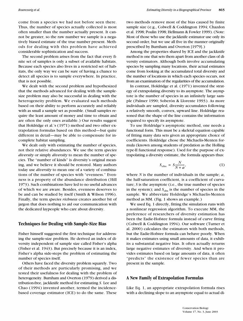
Figure 1. An example of the use of the Michaelis-Menten formula { y � P(x/(x�a))} to estimate diver-sity, where P is the asymptote (and estimate of diversity) and a is the curvature. We loaded a total of 89,596 insects collected from Minnesota habitats into a computer database. The set had 1167 species. We sampled repeatedly from the entire set (with replacement) so as to fashion an accumulation curve. The values plotted (broken line) are averages over all 50 runs. Although the total set contained 1167 species, the average sample of 89,596 individuals accumu-lated only 1018 of them. The Michaelis-Menten curve (thin solid line) fit the sample curve well (R2 � 0.994), but showed systematic deviation. The P was 1049 spe-cies, which is 118 species fewer than were actually present. Data were supplied by E. Siemann (Siemann et al. 1996).



867

Nonrandom Strategies

Our results showed that the random strategy worked ex-tremely well. One could claim that the random strategycheats a bit, however, because at each step it selects its

r

ecoregions from all 110 ecoregions. Hence, no matterhow few ecoregions are in a subset

r

of the 110, the ran-dom method is not limited to the subset but is looking atthe entire set of 110 ecoregions. On the other hand,each estimate comes only from the data of the subset of

r

ecoregions. How can selecting from all 110 cause aproblem?

The answer is that because all 110 ecoregions areavailable each time a subset is chosen, a substantial num-ber of replications will reveal with exaggerated accuracythe average number of species in a subset of

r

ecore-gions. So the random strategy ought to generate lowvariances, smooth accumulation curves, and estimates oftotal diversity that are perhaps better than can be realis-tically expected from real-world data sets (where, ateach step, only the first

r

ecoregions would actually beknown).

To see that, imagine an explorer who knew nothing ofany ecoregion except those he had visited. Especiallywhen he had visited only a few, he might well have ac-cumulated an atypical number of species. A small num-ber would lead to low estimates of the asymptote; alarge number would lead to high estimates. Therefore,before we can gain any confidence in the method, wehave to limit the computer to the sort of knowledge theexplorer would have. We devised several nonrandomstrategies to mimic such an explorer and his increasingknowledge.

We began by specifying the geographical position ofeach ecoregion in a square, virtual space with

x

and

y

coordinates ranging from 1 to 110. We assigned eachecoregion a unique latitudinal integer on the

y

interval.The ecoregion located farthest north received the 1. Theecoregion whose northern-most point was farthestsouth received the 110. Proceeding from west to east,we similarly assigned longitudinal integers to eachecoregion (Fig. 2).

Next we chose ecoregions from which our fictionalexplorer would begin surveying. We selected 21 differ-ent starting points, which we called

kernels

: four eachfrom among the northern, southern, eastern, and west-ern ecoregions and five from ecoregions in the middleof the continent. Thus, we imagined 21 different explor-ers and tried to find out how well each was likely to do.Then we estimated the uncertainty they had to be pre-pared to accept in return for not surveying the entirecontinent. (Details of how we chose the kernels are avail-able at www.evolutionary-ecology.com/data/butterfly.pdf.)

We next produced ordered lists of the 110 ecoregionsfor the explorer to follow. Each began at one of the ker-nels. At each step, our estimators were constrained to

proceed strictly in order through a single list. Thus, theycould not take advantage of any information except thatavailable from the limited subset of ecoregions.

We produced three separate ordered lists for each ker-nel. Each corresponded to one of the following three ex-ploration tactics: blob, cluster, and spread. For the blobtactic we imagine our explorer extending her knowl-edge outward gradually and without skipping overecoregions. One may liken this tactic to a drop of liquidpermeating a blotter in all possible directions. To exe-cute the blob tactic, we calculated the distances from akernel to the other 109 ecoregions. Then we orderedthe distances from smallest to largest. The ordered list ofecoregions associated with these distances became theblob list for that kernel.

For the cluster tactic we imagine our explorer leavingcolonies of explorers behind wherever she goes. At eachstep, she surveys whichever ecoregion is closest to oneof these colonies. Execution of the cluster tactic re-quires the same set of distances calculated for the blobtactic. At each step of the cluster tactic, however, wecalculate the distances from all the chosen ecoregions toall the unchosen ones and then pick the shortest dis-tance. The cluster tactic is similar to the blob tactic be-cause at each step no gaps are allowed between chosenecoregions. But in practice the cluster tactic penetratedthe continent more rapidly than the blob tactic.

For the spread tactic we imagine that at each step ourexplorer deliberately surveys the largest unexploredpart of the continent. Hence, at each step the ecore-

Figure 2. Position of the ecoregions (0–110) in the virtual space (see text). Circles mark ecoregions not selected as kernels. Symbols for ecoregions designated as kernels: boxes, eastern; diamonds, northern; X, western; downward-pointing triangles, southern; solid upward-pointing triangles, central. The entire set roughly resembles the combined shapes of Canada and the continental United States.

868

Estimating Diversity in a Biogeographical Province Rosenzweig et al.


gions that have already been surveyed have intentionallybeen spread out rather uniformly throughout the conti-nent. In probabilistic terms, they are hyperdispersed,the distances separating them from their nearest neigh-bors being less variable than they would be if they werechosen at random. We achieved hyperdispersion as fol-lows. The second ecoregion in each spread list was theone farthest from its kernel ecoregion. To order the re-maining 108 ecoregions, we projected the east-west po-sitions of the already chosen regions onto the x-axis.Then we found the largest

x

gap between selectedecoregions and calculated the

x

value in the center of it.The ecoregion with that value became number three.Next we found the largest gap on the y-axis between se-lected ecoregions and calculated the

y

value in the cen-ter of it. That ecoregion became number four. We re-peated the latter two steps until all 110 ecoregions hadbeen placed in the sampling order. We do not claim thatthis algorithm achieves maximal hyperdispersion at anystage of ordering the list, but it does deviate from ran-domness in the direction of substantial hyperdispersion.

Results

Random Accumulation

The number of species observed (

S

obs

) rose gradually to-ward 561 as more ecoregions were included in the sam-ple. Figure 3 shows the results for one run of 50 replica-tions beginning with a random seed of three, but all runsresembled this one. The jackknife and the ICE—the twoestimators that cannot take advantage of the shape ofthis curve—tracked

S

obs

fairly closely. Their estimates ofhow many species reside in the entire system were onlya bit higher than the number residing in the already sur-veyed ecoregions. This was not true of the four extrapo-lation estimators.

F6 was the least successful extrapolation estimator. Itwas the most erratic, especially when permitted to usefewer than about one-third of the ecoregions. With one-third or more, it flattened out to a modest overestimate ofthe number of butterfly species. It estimated 590 specieswhen given the data of all 110 ecoregions to work with.

We have confidence that this overestimate is an inher-ent property of F6. We are less sure whether its erraticbehavior on the left side of Fig. 3 is an inherent propertyof the formula or derives from the software. The soft-ware performs nonlinear regression automatically in or-der to fit F3, F5, F6, and MM. Because F6 has two param-eters of curvature, it is the most delicate. Inappropriateautomatic choice of initial parameter values can thwartthe attempt of the program to converge to a satisfactorynonlinear regression. Checking this possibility requiresextensive manual analyses whose results would be of lit-tle value.

MM and F3 did much better than F6. On the left side ofFig. 3, their results fluctuated negligibly, especially com-pared with those of F6 (Table 1). With moderate numbers(11–50) of ecoregions in the pooled data, MM showedslightly more negative bias than F3. Using all 110 ecore-gions, MM estimated 579 butterfly species, the most accu-rate of any estimator. With all 110 ecoregions, F3’s estimatewas 588 species. But the end estimate is not very useful.With all 110 ecoregions in hand, one already knows aboutvirtually all the species and no longer needs an estimator.

Where information is least complete and a successfulestimator would be most valuable, F5 did best. F5 reached546 species with the use of only 10 ecoregions. Its ter-minal estimate was 583 species, so it was also the flattestestimator—the one least affected by the proportion ofecoregion lists included. With the use of 11 ecoregions,

Figure 3. Average results of species accumulation and six diversity estimators (50 runs with random shuf-fling of ecoregion order and of occurrences within each successive set of chosen ecoregions). Result type is most readily distinguished over x � 15, where the fol-lowing y values were obtained: accumulation � 369 species; incidence-based coverage estimator (ICE) � 410 species; jackknife method � 431; Michaelis-Menten (MM) method � 508; F3 � 512; F5 � 556; F6 off-scale at 1456 species. All estimators converge over large sample sizes. Unlike the MM curve in Fig. 1, the extrapolation estimators do not follow the numbers of species in the accumulation curve. Instead, the soft-ware utilizes that curve up to a certain number (r) of ecoregions, performs a fit like that of Fig. 1, then re-ports the results of its extrapolation as the y value over that r value. Next, it adds another ecoregion, refits the data, and reports the results of that extrapolation. Re-sults changed little when the random seed was altered or the number of runs was increased greatly. Table 1 reports statistics for a slightly different protocol with similar results.



869

the estimates were F5

�

556, F3

�

512, and MM

�

508(Fig. 3).

In Fig. 3 and similar runs, we asked the software tohave the estimators fit the average values of observed

S

.This gave a good idea of the patterns exhibited by themean extrapolation estimates. But it did not report thevariation in those estimates for any single

r

value (r �number of ecoregions included in the estimate). To ex-amine such variation, we ran 50 replicates and savedeach one separately (Table 1). The means of these re-sults were somewhat different from those of Fig. 3 be-cause the latter uses means for the nonlinear regres-sions, whereas the former regresses the separate resultsand then calculates the mean estimate afterward.

At both r � 11 and r � 22, MM produced the leastvariability, F3 somewhat more, and F5 more still. Thevariability of F6 was large even at r � 22.

The means and medians produced by separating theregressions ranked similarly to those obtained from theprevious single-regression method (Table 1 ). The me-dian of F5 at r � 11 remained superior to the others, butits mean seemed to have acquired a substantial positivebias. At r � 22, the median of F3 was slightly closer to561 than that of F5, but probably not significantly so. Inany case, F5’s estimates of the mean using the single-regression technique were the best of all. Thus, therewould seem to be no need in practice to go to the con-siderable extra trouble of performing separate regres-sions.

Nonrandom Accumulation

As in the case of random accumulation, both the ICE andthe jackknife returned estimates only modestly higher

Table 1. Extrapolation estimates of species diversity with 11 or 22 ecoregions chosen randomly from the full set of 110.*

Includes first 11 ecoregions Includes first 22 ecoregions

F6 F5 F3 MM F6 F5 F3 MM

Minimum 328.4 236.8 234.2 244.7 354.9 418.7 412. 413.0Maximum 3885.6 2660.2 1050.3 915.6 1628.2 840.9 730. 674.7Mean 905.0 668.9 535.9 524.5 749.3 583.4 560.6 542.7Median 622.0 545.4 512.4 514.1 650.6 566.5 557.5 542.8SD 762.6 480.6 165.7 133.6 322.9 94.3 76.2 17.8

*We ran 50 replicates, saved each one, and then averaged the 50 estimates. Results pictured in Fig. 3 come from a slightly different method. Aperfect estimate would have been 561, the total number of species in the set of ecoregions. The median of F5 was the best estimate of diversity.

Figure 4. Two examples of F3 analyses using one clus-ter list (N87) and one blob list (C30). These sorts of lists (see text) accumulate spe-cies irregularly. The N87 cluster list accumulated spe-cies rapidly in the vicinity of its kernel and appeared to be approaching an asymp-tote. Then, at about x � 43, it tapped a group of ecore-gions with a novel set of spe-cies. It rose abruptly and the estimator, F3, responded with large overestimates. The C30 blob list accumu-lated species more steadily and never seemed to ap-proach an asymptote. That led to steadily rising F3 overestimates. The F5 and Michaelis-Menten analyses of N87 and C30 behaved similarly.

870 Estimating Diversity in a Biogeographical Province Rosenzweig et al.


than the actual number of species observed at each step.They did this no matter how irregular the shape of theraw accumulation curve because neither of these estima-tors depends on the shape of that curve. The other fourestimators do, however, and their success depends onthe accumulation curve rising reliably toward the trueasymptote.

When ecoregions were sampled in fixed order insteadof random order, the accumulation curve of observed

species did not always resemble a smooth curve ap-proaching an asymptote. In particular, both cluster andblob tactics produced shapes quite different from asmooth approach to an asymptote (Fig. 4). They did sobecause they focus their early samples in a single por-tion of the continent.

For some of these lists, the curve of observed speciesrapidly accumulated the species of that region and lev-eled off because the ecoregions being added werenearby and rather similar in species composition. Thatcircumstance created an early, false appearance of level-ing off. The extrapolation estimators detected it and, atfirst, returned very low estimates of total diversity. Be-yond some r value, the ecoregion lists being added be-gan to tap into ecoregions whose species overlappedvery little with those previously chosen. Observed diver-sity began to climb more rapidly. The raw curve’s accu-mulation rate got steeper, and the extrapolation estima-tors revised their estimates upward.

For other lists, gradual expansion outward from a ker-nel ecoregion led to steady, nearly linear growth in thenumber of species observed (Fig. 4). This too caused allextrapolation estimators to behave badly. They werelooking for an asymptote that always seemed farther andfarther away.

In short, no estimator did a useful job when it wasbased on blob or cluster tactics of ecoregion explora-tion.

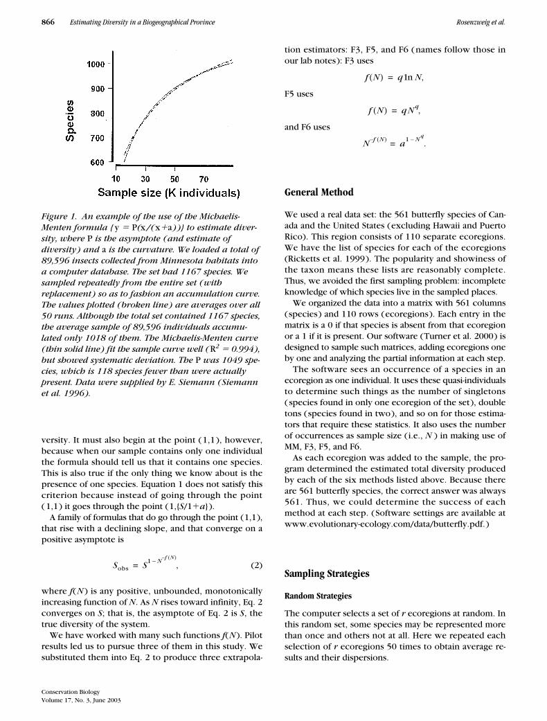
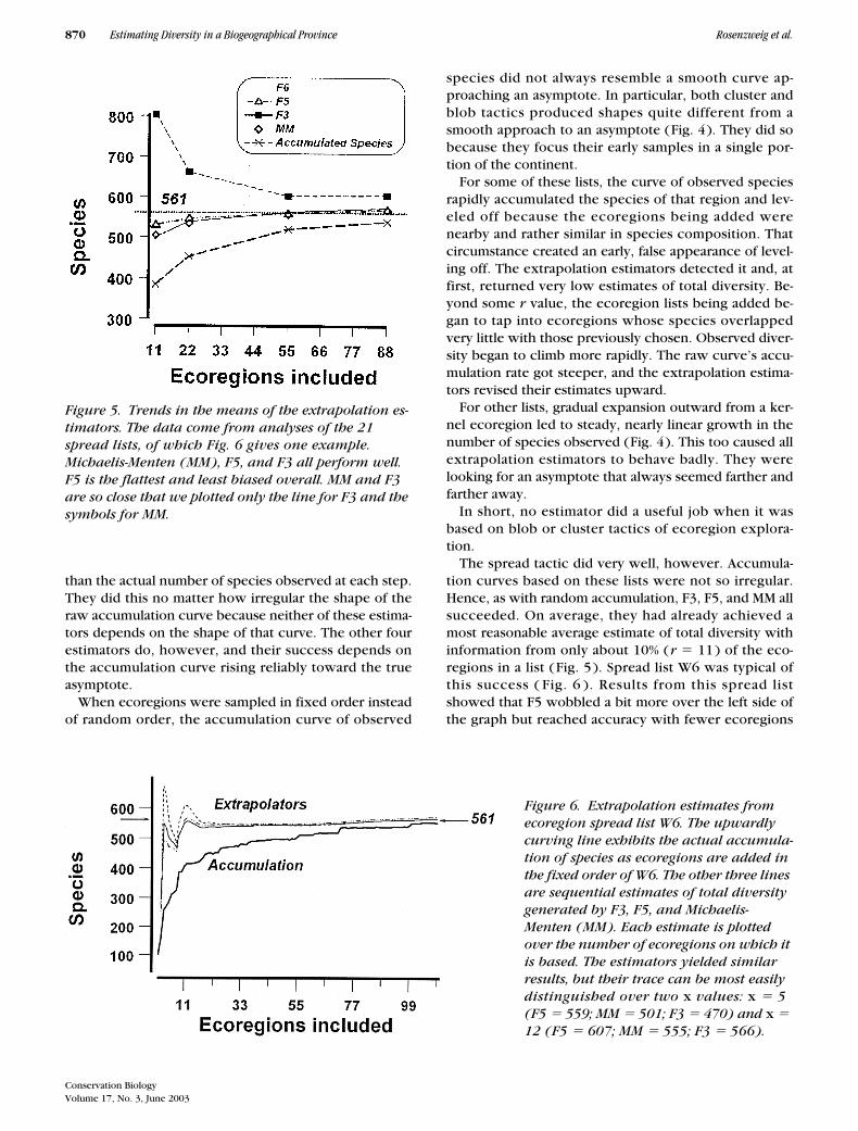
The spread tactic did very well, however. Accumula-tion curves based on these lists were not so irregular.Hence, as with random accumulation, F3, F5, and MM allsucceeded. On average, they had already achieved amost reasonable average estimate of total diversity withinformation from only about 10% (r � 11) of the eco-regions in a list (Fig. 5 ). Spread list W6 was typical ofthis success ( Fig. 6 ). Results from this spread listshowed that F5 wobbled a bit more over the left side ofthe graph but reached accuracy with fewer ecoregions

Figure 5. Trends in the means of the extrapolation es-timators. The data come from analyses of the 21 spread lists, of which Fig. 6 gives one example. Michaelis-Menten (MM), F5, and F3 all perform well. F5 is the flattest and least biased overall. MM and F3 are so close that we plotted only the line for F3 and the symbols for MM.

Figure 6. Extrapolation estimates from ecoregion spread list W6. The upwardly curving line exhibits the actual accumula-tion of species as ecoregions are added in the fixed order of W6. The other three lines are sequential estimates of total diversity generated by F3, F5, and Michaelis-Menten (MM). Each estimate is plotted over the number of ecoregions on which it is based. The estimators yielded similar results, but their trace can be most easily distinguished over two x values: x � 5 (F5 � 559; MM � 501; F3 � 470) and x � 12 (F5 � 607; MM � 555; F3 � 566).


Rosenzweig et al. Estimating Diversity in a Biogeographical Province 871

and held that accuracy as ecoregions accumulated. Withall 110 ecoregions in the sample, F5 � 566, F3 � 571,and MM � 565. F6, the least successful extrapolation es-timator, does not appear in Figs. 5 or 6. It producedoverestimates as high as 3112 species on the left sideand ended with an estimate of 590 species with all 110ecoregions accounted for.

Because each spread list generates a separate set of re-sults, spread lists produce estimates of variability withno special extra work. Their estimates of variabilitywere much less variable then the estimates derived fromrandom lists ( Table 2 ). This reduction in variabilityprobably comes from the nonrandom rules used to gen-erate spread lists. However, the mean and median esti-mates of F3 and MM from spread lists had a greater nega-tive bias than those from random lists. And the meanand median estimates of F5 from spread lists had a nega-tive bias, whereas those from random lists appeared toshow either no bias or a positive bias. In other words,spread lists did not generate estimates as close to 561 asrandom lists did. This negative bias did not characterizeestimates from F6, but F6 had a much greater variabilitythan the others and its estimates were not good enoughto merit further mention.

Results from Combining Methods

To obtain the results reported above, we analyzed eachof the 21 spread lists separately but in strict order. Spe-cies from the second region of each list were added tothose of the first, then those of the third, and so forth.This inevitably led to considerable irregularity in the ac-cumulation curves. They are much less smooth thanthose generated by the random-order method. ( Fig. 6shows an example.) Because of the strict order, our rep-lications could not smooth the accumulation curvesmuch, and we reported results from only 10 runs. Wedid wonder, however, whether we could improve theestimates from spread lists and further reduce their vari-ability by combining the realism of the spread tacticwith the smoothing power of random sampling.

Because random accumulation yielded considerableaccuracy with only 10% of the ecoregions, we smoothed

using the first 10% of the ecoregions in each spread list.We extracted the species occurrence records of the first11 ecoregions in each of the 21 spread lists. Then wesubjected each of these truncated lists to random analy-sis. This is quite a natural way to proceed. One mayimagine that the explorer, having completed the first 11ecoregion surveys, analyzes the results with the randomtactic.

The first 11 ecoregions of a spread list can be listed in11! orders. Each random run selects one of these orders.We executed 50 runs per list, which greatly smoothedthe 21 raw accumulation curves (Fig. 7 shows twoexamples). The smoothing reduced the variance of allthree estimators (Table 3). (The significance of this re-duction is not at issue; we know a priori why it has tohappen.) Although the reduction is small, it comes at noextra analysis or surveying cost.

Table 2. Extrapolation estimates of species diversity with 11 or 22 ecoregions chosen in fixed, hyperdispersed order (“spread lists”) from the full set of 110.*

Includes first 11 ecoregions Includes first 22 ecoregions

F6 F5 F3 MM F6 F5 F3 MM

Minimum 400.0 408.1 407.5 419.7 444.3 459.8 463.7 472.4Maximum 2523.7 805.4 650.4 638.7 1072.1 636.1 617.6 600.4Mean 804.0 530.5 500.7 504.9 660.8 546.6 539.3 533.7Median 602.6 511.8 490.1 498.0 617.5 549.8 544.3 537.1SD 536.3 100.0 68.0 59.0 164.4 48.6 43.0 35.7

*We ran 10 replicates of each of the 21 spread lists and then took statistics on the pool of their estimates. A perfect estimate remained 561 spe-cies. F5, F3, and MM all performed well but exhibited a more negative bias than the estimates from random trials.

Figure 7. Estimating diversity from the first 11 ecore-gions of two spread lists, E12 and E98. One occurrence is a single species in a single ecoregion. We ran each list 50 times, shuffling its ecoregion order to smooth the accumulation curves. Then we fit F5 to obtain their asymptotes. E12 yielded a low estimate, 549 spe-cies, and E98 yielded an unusually high estimate of 714. Symbols show the average total number of occur-rences at each step. Lines show the F5 regressions.



More important than the smoothing, MM, F3, andF5 all now produced reasonably accurate average esti-mates of total diversity (including the species in the un-sampled 99 ecoregions) when the random tactic oper-ated on the occurrence records of the first 10% of theecoregions in each spread list. F3 and MM tended to un-derestimate diversity a bit and F5 to overestimate it( Table 3).

Discussion

Can estimators of species diversity that compensate forsmall sample sizes also compensate for incomplete ex-ploration of habitat types? We put this question to six es-timators of species diversity. In particular, we testedwhether they could produce worthwhile estimates of to-tal butterfly species diversity in a continental-scale re-gion (Canada and the United States).

Those of the six estimators that operate by samplingspecies abundance distributions ( Burnham and Over-ton’s jackknife and Lee and Chao’s ICE) failed our tests.The other four operate by extrapolating the asymptoteof a sequence of diversity accumulations. Three ofthese—MM (based on a simple Michaelis-Menten formula)and F3 and F5 (based on a new family of asymptotic for-mulas) succeeded. The remaining extrapolation formula,F6, based on the very same family, failed.

Provided with only 10% ( i.e., 11) of the species listsfrom ecoregions, the three successful extrapolation esti-mators—MM, F3, and F5—did a remarkable job. Using acombination of tactics that mimics how a real investiga-tor might work, they produced median estimates within4.7%, 3.7%, and 2.4%, respectively, of the actual value(561 species ). The best of these, F5, returned an esti-mate between 551 and 614 species in 95% of cases. ForF3 the confidence interval was 514–560, and for MM itwas 512–554.

The tactics of sequential exploration proved impor-tant. The investigator who begins at one place and grad-ually explores from there is likely to fail, even using thebest extrapolation estimator. Exploration sites may beadded gradually, but their locations must not be clus-tered. They should at least be chosen randomly withinthe total area under investigation. Better even than ran-dom siting was the spread tactic, in which locationswere added so that exploration sites were always spreadrather uniformly through the total area.

The residual variation in estimated diversity arosefrom the variation in total species accumulated by thefirst r ecoregions in a spread list. Total species accumu-lated ( Sobs ) correlated positively with diversity esti-mates. (Regression results: F3 prediction for the first 11ecoregions of the 21 spread lists regressed on Sobs,p � 10�5, R2 � 0.65; F5 prediction on Sobs, p � 10�3,R2 � 0.46; MM prediction on Sobs, p � 10�5, R2 � 0.64.)We found no way to eliminate that correlation, not evenby increasing the number of ecoregions included. Never-theless, the extrapolation estimators we studied gave agood empirical picture of the value of true S.

The primary difference between the three successfulestimators and the fourth extrapolation estimator (F6)is that F6 has two parameters of curvature (a and q) in-stead of only one. Despite that extra parameter of cur-vature, F6 failed to extrapolate to the true diversity,whereas the other three extrapolators—each with onlyone parameter of curvature—succeeded. We do notunderstand why F6 did not do as well as the otherthree.

We also cannot explain why MM did succeed. TheMichaelis-Menten formula (on which MM is based) hasa built-in error. It does not go through the point (1,1), apoint that characterizes every diversity sample with asingle individual. Perhaps this error should have beena heavy burden for MM, but it was not. Is MM’s successlimited to large ecoregions containing many species?Will MM’s intrinsic error be more consequential whenestimates are being made at smaller scales with relativelysmall amounts of information?

We believe that we do understand the failures of thejackknife and ICE estimators. These two were designedto overcome sample-size inadequacies and to reveal howmany species are present in habitats actually sampled.Our results do not challenge their success at doing thisjob. But neither one was designed for extrapolation.They operate only on the results obtained from a partic-ular subset of the total data set. They pay no attention tothe pathway along which that subset was accumulated.But that pathway is what must contain the informationneeded to reveal the asymptote of diversity. And thatpathway is the very pathway that the extrapolation for-mulas are meant to fit.

F3 and F5 are hybrids. They combine deductive rea-soning with empiricism. A priori reasoning tells us that a

Table 3. Extrapolation estimates of species diversity with ecoregions limited to the first 11 of each of the 21 “spread-lists.”*

Speciesin sample F5 F3 MM

Minimum 326.3 448.7 431.5 436.2Maximum 425.8 727.3 625.1 613.2Median 392.3 574.2 540.5 534.6Mean 386.9 582.3 537.0 533.0SD 26.4 68.9 50.8 45.895% confidence interval 31.4 23.1 20.8

*We ran 50 replicates of each of the 21 spread lists and then calcu-lated statistics on the pool of their 21 average estimates. In each ofthe 1050 analysis runs, ecoregion order was shuffled randomly. Aperfect estimate remained 561 species. The median estimates of F5,F3, and MM were all quite close to 561, despite the limited sample.F5 tended to overestimate diversity. MM and F3 tended to underesti-mate it.


Rosenzweig et al. Estimating Diversity in a Biogeographical Province 873

successful formula must begin at the point (1,1) and risemonotonically toward an asymptote. Data tell us that thesecond derivative of any successful formula must be neg-ative throughout. (Some formulas conforming to Eq. 2produce curve segments with positive second deriva-tives; we did not include them in this report. ) And, ofcourse, the data are the ultimate judges of F3 and F5. Ex-cept for its failure to traverse the point (1,1), MM alsocombines these same deductive and empirical compo-nents.

In arriving at F3 and F5, we included no assumptionsexcept to begin at the point (1,1 ) and rise monotoni-cally toward an asymptote. In particular, neither formulaassumes a specific distribution of abundances (such aslog series or lognormal), which we believe is a strength.Just as many processes produce linear relationships (thusfitting the general skeletal equation, y � mx � b), so F3and F5 will fit many curves that rise to an asymptotefrom the point ( 1,1 ) (as will F6, although it servedpoorly for diversity extrapolation).

No formula passes muster merely by making good the-oretical sense. The data must also support it. The centralrole of the data in arriving at our conclusions is incontro-vertible. Having no complete deductive scheme to pre-dict our extrapolation formulas, we must admit thattheir excellent fit to the butterflies of North Americamight turn out to be unusual. More real data from othertaxa and other provinces will prove essential to accep-tance of the methods. The present results, however,seem promising.

The butterfly data come from the large scale of wholeecoregions. Moreover, they are quite unusually com-plete. Does successful extrapolation depend on largescale and fairly complete knowledge of some of its com-ponents? We have no answer to the question of scale,but complete knowledge of components may not be es-sential. Bias-reducing estimators such as ICE and thejackknife efficaciously tell us how many species residein a given patch of space-time. A hyperdispersed seriesof such patches could be operated on by such estima-tors to produce good estimates of diversity within eachpatch. If we could extract from such data an estimate ofspecies overlap from ecoregion to ecoregion, then, oper-ating on a growing set of patches, the present extrapola-tion formulas could produce an estimate of the asymp-tote. The extrapolation ought to be valid for the wholearea within which the samples have been selected.

We used only geographical location to organize the(hyperdispersed) spread lists. Would it have been betterto rely on the biologically relevant properties of a place,for example, its temperature and rainfall? We doubt it.One can usually get such data for large scales every-where, but not for microscales. If we had used a biologi-cally meaningful set of variables to sort ecoregions, wemight have raised an impediment to use of the tech-nique at microscales. Thus, we are particularly encour-

aged that the simple tactic of spreading the sampling lo-cations worked well.

The practical application of the method requires ananswer to at least one other question. How many sub-samples are enough? We found that a 10% sample wasenough, but that answer may not always be correct. Inpractice, moreover, it may be difficult to tell when 10%is reached (especially at smaller scales). We are activelyworking on developing an internal statistic to answerthis question. A promising candidate involves the ratioof accumulated species to estimated species.

A successful extrapolation estimator will have manyuses. It will greatly reduce the time and resources requiredto obtain reliable diversity totals (Heywood 1995). It willallow diversity to be estimated at fine temporal scales sothat conservation biologists can better track its dynam-ics (Devries et al. 1999). It should manifestly improvethe ability of paleobiologists to overcome the incom-pleteness of the fossil record and so better allow them todiscern any patterns of change in diversity in the historyof life (Lee 1997). Finally, it will at last enable ecolo-gists to estimate worldwide species diversity (Gaston& Hudson 1994; Rosenzweig 1995).

Acknowledgments

A portion of this paper is derived from the University ofArizona senior honors thesis of J. G. Cox. E. Siemannfurnished the data for Fig. 1. We thank H. Possingham,G. Meffe and E. Main for suggestions that improved themanuscript.

Literature Cited

Burnham, K. P., and W. S. Overton. 1979. Robust estimation of popula-tion size when capture probabilities vary among animals. Ecology60:927–936.

Chazdon, R. L., R. K. Colwell, J. S. Denslow, and M. R. Guariguata.1998. Statistical methods for estimating species richness of woodyregeneration in primary and secondary rain forests of northeasternCosta Rica. Pages 285–309 in F. Dallmeier and J. A. Comiskey, edi-tors. Forest biodiversity research, monitoring and modeling: con-ceptual background and old world case studies. Volume 20. UnitedNations Environmental, Scientific, and Cultural Organization, Paris,and Parthenon Publication, New York.

Colwell, R. K., and J. A. Coddington. 1994. Estimating terrestrial biodi-versity through extrapolation. Philosophical Transactions of theRoyal Society of London Series B 345:101–118.

Devries, P. J., T. R. Walla, and H. F. Greeney. 1999. Species diversity inspatial and temporal dimensions of fruit-feeding butterflies fromtwo Ecuadorian rainforests. Biological Journal of the Linnean Soci-ety 68:333–353.

Fisher, R. A., A. S. Corbet, and C. B. Williams. 1943. The relation be-tween the number of species and the number of individuals in arandom sample of an animal population. Journal of Animal Ecology12:42–58.

Gaston, K. J., and E. Hudson. 1994. Regional patterns of diversity andestimates of global insect species richness. Biodiversity and Conser-vation 3:493–500.



Hellmann, J. J., and G. W. Fowler. 1999. Bias, precision, and accuracyof four measures of species richness. Ecological Applications 9:824–834.

Heywood, V. H. 1995. Global biodiversity assessment. United NationsEnvironment Programme, Cambridge, United Kingdom.

Hill, M. O. 1973. Diversity and evenness: a unifying notation and itsconsequences. Ecology 54:427–431.

Holdridge, L. R., W. C. Grenke, W. H. Hatheway, T. Liang, and J. A.Tosi. 1971. Forest environments in tropical life zones. PergamonPress, Oxford, United Kingdom.

Lee, M. S. Y. 1997. Documenting present and past biodiversity: conser-vation biology meets palaeontology. Trends in Ecology & Evolution12:132–133.

Lee, S.-M., and A. Chao. 1994. Estimating population size via sample cov-erage for closed capture-recapture models. Biometrics 50:88–97.

Palmer, M. W. 1990. The estimation of species richness by extrapola-tion. Ecology 71:1195–1198.

Poulin, R. 1998. Comparison of three estimators of species richness

in parasite component communities. Journal of Parasitology 84:485–490.

Ricketts, T. H., E. Dinerstein, D. M. Olson, C. Loucks, W. Eichbaum,K. Kavanagh, P. Hedao, P. Hurley, K. M. Carney, R. Abel, and S. Walters.1999. Terrestrial ecoregions of North America: a conservation assess-ment. Island Press, Washington, D.C.

Rosenzweig, M. L. 1995. Species diversity in space and time. Cam-bridge University Press, Cambridge, United Kingdom.

Siemann, E., D. Tilman, and J. Haarstad. 1996. Insect species diversity,abundance and body size relationships. Nature 380:704–706.

Smith, B., and J. B. Wilson. 1996. A consumer’s guide to evenness indi-ces. Oikos 76:70–82.

Soberón, J., and J. Llorente. 1993. The use of species accumulationfunctions for the prediction of species richness. Conservation Biol-ogy 7:480–488.

Turner, W., W. A. Leitner, and M. L. Rosenzweig. 2000. Ws2m.exe.University of Arizona, Tucson. Available at http://eebweb.arizona.edu/diversity (accessed 31 March 2003).

estimating diversity in unsampled habitats of a ... · ecoregiones. las buenas estimaciones...

Documents