estimating depth to bedrock in weathered terrains using ... · ground-penetrating radar (gpr) is a...
TRANSCRIPT

Estimating depth to bedrock in
weathered terrains using ground-
penetrating radar: a case study in the
Adelaide Hills
Thesis submitted in accordance with the requirements of the University of Adelaide for
an Honours Degree in Geophysics
Dylan Cremasco
November 2013
Bedrock depth estimation using ground-penetrating radar 1
TITLE Estimating depth to bedrock in weathered terrains using ground-penetrating radar: a
case study in the Adelaide Hills
RUNNING TITLE
Bedrock depth estimation using ground-penetrating radar
ABSTRACT
Ground-penetrating radar (GPR) is a geophysical technique that is commonly applied to
a variety of subsurface investigations, with the capability to determine depth to bedrock
under favourable soil conditions. This study was conducted at three different
physiographic regions that represent typical terrains in the Adelaide Hills. At each site,
GPR surveys were conducted along traverses using 100, 250, 500 and 800 MHz
antennae. A drilling program was conducted concurrently with the GPR survey to
provide baseline bedrock depths for comparison. Electrical resistivity and
electromagnetic surveys were also conducted along each traverse to determine
subsurface conductivity and secondary bedrock depth estimates. The GPR results for all
antennae were compared to determine the frequency that provided the best depth
estimation. Rapid attenuation of GPR signal at all frequencies was observed, resulting
in shallower than expected investigation depths. At two of the sites, GPR signal
penetration depth was increased in areas that were highly resistive. The 800 MHz
antennae displayed the highest resolution of estimated bedrock contacts in these
resistive areas, and were subsequently compared to drill refusal depths using a paired t
test. GPR estimation depths and drill refusal in electrically resistive areas strongly
correlated at two of the sites, while the third site showed no correlation. Across all three
transects bedrock depths were underestimated by 74% on average. This underestimation
is attributed to signal attenuation, which appears to be caused by a combination of
increased conductivity, clay content and the presence of iron oxides in the soil profile.
Without further investigation it is difficult to quantify these factors on attenuation in the
area. The results of this study suggest that GPR surveys are not suitable for bedrock
depth estimation in Adelaide Hills-type terrains.
KEYWORDS
Ground-penetrating radar, bedrock depth, Adelaide Hills, site productivity, soil profile,
attenuation

Bedrock depth estimation using ground-penetrating radar 2
TABLE OF CONTENTS
List of Figures ............................................................................................................... 3
List of Tables ................................................................................................................ 4
1. Introduction .............................................................................................................. 6
2. Geological setting ................................................................................................... 10
2.1. Regional tectonic history ................................................................................. 10
2.2. Local geology .................................................................................................. 11
2.3. Study area ....................................................................................................... 12
2.3.1. Site 1: Rocky Paddock ............................................................................. 12
2.3.2. Site 2: Chalkies Line ................................................................................ 13
2.3.3. Site 3: Canham Road ............................................................................... 14
3. Equipment theory .................................................................................................... 16
3.1. Ground-penetrating radar ................................................................................. 16
3.2. Electrical resistivity ......................................................................................... 20
3.3. Electromagnetics ............................................................................................. 21
4. Methods .................................................................................................................. 22
4.1. Ground-penetrating radar ................................................................................. 22
4.2. Electrical resistivity ......................................................................................... 23
4.3. Electromagnetics ............................................................................................. 24
4.4. Drilling and soil analysis ................................................................................. 25
5. Observations and results .......................................................................................... 26
5.1. Site 1: Rocky Paddock ..................................................................................... 27
5.2. Site 2: Chalkies Line ....................................................................................... 32
5.3. Site 3: Canham Road ....................................................................................... 38
6. Discussion ............................................................................................................... 43
6.1. GPR Signal Attenuation .................................................................................. 45
6.1.1. Signal scattering ...................................................................................... 45
6.1.2. Soil conductivity ...................................................................................... 46
6.1.3. Clay content............................................................................................. 47
6.1.4. Iron oxide content .................................................................................... 48
6.2. Signal attenuation summary ............................................................................. 49
7. Conclusions ............................................................................................................ 50
8. Acknowledgments ................................................................................................... 51
9. References .............................................................................................................. 51
Appendix A: Detailed methods ................................................................................... 55

Bedrock depth estimation using ground-penetrating radar 3
Appendix B: Soil Analysis Data .................................................................................. 60
Appendix C: GPR radargrams for Site 1...................................................................... 75
Appendix D: GPR radargrams for Site 2 ..................................................................... 80
Appendix E: GPR radargrams for Site 3 ...................................................................... 85
LIST OF FIGURES
Figure 1: Locality map of the three survey lines within the Mount Crawford Forestry
Reserve. ...................................................................................................................... 13
Figure 2: Topographic cross-section of the traverse at Site 1 (Rocky Paddock) ......... . 14
Figure 3: Topographic cross-section of the traverse at Site 2 (Chalkies Line). ............. 15
Figure 4: Topographic cross-section of the traverse at Site 3 (Canham Road). ............. 15
Figure 5: Schematic diagram of potential radio wave propagation paths generated by a
GPR transmitter. ......................................................................................................... 16
Figure 6: Cross-section of the Site 1 traverse. Drill hole locations and depths are marked
relative to regional topography. ................................................................................... 27
Figure 7: Comparative plot of processed ground-penetrating radar data for Site 1
(Rocky Paddock)......................................................................................................... 28
Figure 8: Comparison plot for Site 1 ........................................................................... 30
Figure 9: Cross-section of the Site 2 traverse. Drill hole locations and depths are marked
relative to regional topography. ................................................................................... 32
Figure 10: Comparative plot of processed ground-penetrating radar data for Site 2
(Chalkies Line) ........................................................................................................... 33
Figure 11: Comparison plot for Site 2 ......................................................................... 35
Figure 12: Cross-section of the Site 3 traverse. Drill hole locations and depths are
marked relative to regional topography. ...................................................................... 38
Figure 13: Comparison plot of processed ground-penetrating radar data for Site 3
(Canham Road) ........................................................................................................... 39
Figure 14: Comparison plot for Site 3 ......................................................................... 41

Bedrock depth estimation using ground-penetrating radar 4
LIST OF TABLES Table 1: Operational parameters of all GPR antennae used at each site........................ 23
Table 2: Receiver array orientations and depths of investigation for the DualEM-421
instrument. .................................................................................................................. 24
Table 3: Paired t-test to establish mean value and Pearson correlation between drill
refusal depth and GPR bedrock depth estimates at Site 1. ............................................ 31
Table 4: Paired t-test to establish mean value and Pearson correlation between drill
refusal depth and GPR bedrock depth estimates at Site 1, using only data from locations
in areas with large scale resistive subsurface. .............................................................. 31
Table 5: Paired t-test to establish mean value and Pearson correlation between drill
refusal depth and GPR bedrock depth estimates at Site 2. ............................................ 37
Table 6: Paired t-test to establish mean value and Pearson correlation between drill
refusal depth and GPR bedrock depth estimates at Site 2, using only data from locations
in areas with large scale resistive subsurface. .............................................................. 37
Table 7: Paired t-test to establish mean value and Pearson correlation between drill
refusal depth and GPR bedrock depth estimates at Site 3. ............................................ 43
Table 8: Paired t-test to establish mean value and Pearson correlation between drill
refusal depth and GPR bedrock depth estimates at Site 3, using only data from locations
in areas with large scale resistive subsurface. .............................................................. 43

Bedrock depth estimation using ground-penetrating radar 5
This page is intentionally blank

Bedrock depth estimation using ground-penetrating radar 6
1. INTRODUCTION
The depth to bedrock from the ground surface, and therefore the thickness of the
overlying soil, strongly correlates with the distribution of horizons within a soil profile.
Soil physical and chemical properties, such as groundwater interactions, sub-soil water
movement, water storage and nutrient availability are all factors that are controlled by
the horizon distribution and thickness (Sucre et al. 2010). The overall productivity of a
site is regulated by these soil properties (Wilford & Thomas 2012). Typically, a soil
profile includes the A, B and C horizons (Fitzpatrick 1988). Moderately weathered
bedrock below the C horizon is recognised as the R horizon (McDonald & Isbell 2009).
The depth to this R horizon is considered in soil science to represent the contact point
between the soil profile and underlying bedrock (Fitzpatrick 1988, McDonald & Isbell
2009). Determining the depth to the R horizon can provide essential information about a
soils properties when investigating potential land uses (Sucre et al. 2010, Wilford &
Thomas 2012).
Depth to bedrock is commonly measured by traditional mechanical methods. These
ground truthing practises include augering, coring and excavation (Collins & Doolittle
1987). All of these techniques are time consuming, expensive and often result in high
levels of soil disturbance (Collins & Doolittle 1987). Ideally, a cheaper, more accessible
and less destructive ground truthing method is required. Determining depth to bedrock
using shallow geophysical techniques has been documented in a variety of terrains
(Davis & Annan 1989, Jol & Smith 1991, Wightman et al. 1992, Triantafilis &
Buchanan 2009, Sucre et al. 2010, Coulouma et al. 2011). The use of these techniques
within the erosional landscapes of the Adelaide Hills for bedrock depth estimation has

Bedrock depth estimation using ground-penetrating radar 7
not been previously investigated. Due to the varying limitations and conditional
requirements of geophysical equipment, the effectiveness of applied methods will vary
depending on the style of landscape and the underlying soil profile (Samouelian et al.
2004, Sucre et al. 2010). Previous work suggests that ground-penetrating radar (GPR)
holds the potential to accurately estimate depth to bedrock in complex weathered
terrains (Doolittle & Collins 1995), such as those seen in the Adelaide Hills region. The
speed, cost and ease of data acquisition make GPR an attractive method for bedrock
depth estimation. The use of GPR under favourable conditions has been found to reduce
field cost by up to 70%, and increase efficiency by 210% (Doolittle & Collins 1995).
The successful application of GPR is dependent on the physical and chemical
characteristics of the subsurface, such as bulk conductivity and presence of clay
(Olhoeft 1986, Du & Rummel 1994, Doolittle & Collins 1995, Reynolds 1997). These
factors control the overall quality of signal transmission and reflection (Saarenketo
1998). Optimal subsurface conditions for GPR include electrically resistive sands,
gravels and clastic sediments (Jol & Smith 1991, Jol & Bristow 2003). Incompatible
soils result in the loss of transmitted GPR signal (Olhoeft 1986, Doolittle & Collins
1995). This signal loss, called attenuation, minimises the total depth of GPR survey
investigation (Reynolds 1997, Annan 2005). Sucre et al. (2010) investigated the use of
GPR for bedrock depth estimation within the Southern Appalachian Mountains,
concluding it to be an effective technique, though highly dependent on the electrical
conductivity of the overlying soils. GPR surveys have been conducted for a wide range
of applications in Australia, with only a limited number of these regarded as being
successful (Griffin & Pippet 2002). Soils occurring within Australia tend to be more
Bedrock depth estimation using ground-penetrating radar 8
conductive than those found in other countries, reducing the effectiveness of GPR
surveys (Griffin & Pippet 2002, McDonald & Isbell 2009). Taking these findings into
account, other forms of geophysical investigation should be considered to provide
additional subsurface information in any areas in which the GPR signal becomes
attenuated. Two common shallow ground geophysical techniques for measuring soil
conductivity include electrical resistivity surveys and electromagnetic (EM) surveys
(Kearey et al. 2002, Fitterman & Labson 2005, Zonge et al. 2005). High soil
conductivity readings from these techniques can potentially provide an explanation for
unexpected GPR signal attenuation.
Electrical resistivity techniques aim to determine the resistivity of the surrounding soil
volume (Samouelian et al. 2004, Zonge et al. 2005). Electrical resistivity of soil
volumes can be considered as a proxy for the variability of a variety of soil properties;
such as structure and water content (Banton et al. 1997, Samouelian et al. 2004). The
use of electrical resistivity surveying for bedrock depth estimation is greatly influenced
by the contrast in electrical resistivity between the soils and underlying bedrock
(Coulouma et al. 2010, Coulouma et al. 2011). Low electrical resistivity contrast
between the soil and underlying bedrock results in a low resolution contact point on the
resistivity imaging, providing less accurate bedrock depth estimations (Banton et al.
1997, Coulouma et al. 2011). The ability of these systems to provide useful information
on the subsurface conductivity distribution, while providing an alternate method of
bedrock depth detection, makes them a desirable instrument to include in this survey.
EM survey methods are commonly used to map near-surface geology by tracing
variations in the electrical conductivity properties of underlying rocks and soils

Bedrock depth estimation using ground-penetrating radar 9
(Doolittle et al. 1994, Fitterman & Labson 2005). Similar to electrical resistivity,
electromagnetic variations are generally controlled by soil and rock structure, porosity,
clay content, groundwater salt content and water saturation (McNeill 1990, Doolittle et
al. 1994). EM surveys are commonly employed for groundwater, salinity and clay
profiling (McNiell 1980, Doolittle et al. 1994), though the potential of mapping
sedimentary stratigraphy and bedrock contacts has been investigated. Electromagnetic
response analysis for a multi-layered earth model conducted by McNiell (1980) found
shallow terrain conductivity meters, like the Geonics EM-31 system, to be theoretically
capable of mapping soil-bedrock contacts when high conductivity contrasts are present
at the interface between the two materials. Frequency domain electromagnetic surveys
(FDEM) conducted by Wightman et al. (1992) showed highly conductive shale bedrock
to be modelled by the technique through up to 15 m of overburden. FDEM surveys
conducted by Triantafilis and Buchanan (2009) along the Darling River valley were
used for the purpose of mapping near surface and sub-surface stratigraphic units. The
results were used to interpret soil clay content, cation exchange capacity and soil
electrical conductivity. These estimations can provide useful information for this study,
as such properties often are associated with the soil profile thickness and type of
bedrock present (Wightman et al. 1992).
This work evaluates the suitability of GPR to provide depth to bedrock measurements
within the complex and weathered terrains of the Adelaide Hills. Study sites were
chosen within the Mount Crawford Forestry Reserve, South Australia. In order to test
the versatility of the approach across variable terrains and parent materials, survey lines
were selected within three contrasting physiographic regions. Ground truthing data were

Bedrock depth estimation using ground-penetrating radar 10
also collected by using traditional drilling methods for direct comparison to GPR survey
results. EM and electrical resistivity survey results are also compared to GPR and
ground truthing data. By analysing these comparisons, this study aims to provide insight
into the ability of GPR to estimate depth to bedrock in this type of terrain.
2. GEOLOGICAL SETTING
2.1 Regional tectonic history
The Mount Crawford Forestry Reserve is a grouping of several native and plantation
forests surrounding the Mount Crawford area, located within the central Mount Lofty
Ranges in South Australia. Tokarev (2005) identifies the Mount Lofty Ranges to be the
result of a complex neotectonic deformational history in the region; specifically an
extensional regime (Middle Eocene to Middle Miocene), a transitional stage (Late
Miocene to Early Pleistocene) and a compressional regime (Early Pleistocene to
present). Crustal segmentation in the region during the later stages of the Eocene
resulted in the subsidence of the surrounding St. Vincent and Western Murray Basins
(Sandiford 2002, Tokarev 2005). The central palaeoplain between the subsiding basins
shaped what would eventually become the Mount Lofty Ranges (Benbow et al. 1995).
The influence of a compressional neotectonic regime caused the formation of steep
reverse faulting on either side of the palaeoplain (Tokarev 2005). These fault scarps
align along a roughly north-south line and persist throughout the length of the ranges
(Bourman & Lindsay 1989, Sandiford 2002). Uplift of the central palaeoplain caused by
the compressional regime lead to the formation of the Mount Lofty Ranges (Sandiford
2002, Tokarev & Gostin 2003). The uplift of the Ranges primarily occurred during the

Bedrock depth estimation using ground-penetrating radar 11
Pleistocene, with present day in-situ stress measurements and seismic activity indicating
the continuing uplift of the area (Sandiford 2002, Tokarev 2005).
2.2 Local geology
The Palaeoproterozoic Barossa Complex of the Houghton Inlier forms the basement
underneath the Mount Lofty Ranges (Preiss 1987). The basement is unconformably
overlain by Adelaidean metasediments, forming an approximately 7 km thick cover
over the region (Preiss 1987). During the Cambrian Delamerian Orogeny, the
Adelaidean sediments were metamorphosed to greenschist facies (Preiss et al. 2008).
The Warren Inlier, an anticlinal core of pre-Adelaidean basement, is located within the
metamorphosed sediments (Preiss et al. 2008). The Aldgate sandstone that overlies the
Mount Crawford area passes eastward into the Springfield Shear Zone (Preiss 1987).
Structurally overlying the Aldgate Sandstone is the highly deformed micaceous
feldspathic meta-siltstones and meta-sandstones of the Cambrian Kanmantoo Group
(Preiss et al. 2008, Wilford & Thomas 2012). Two differing perspectives on the source
of the highly deformed micaceous schist have been theorised: Conor (1984) described
polyphase deformation of Adelaidean metasediments to be the source. Conversely,
Townsend (1984) identified similarities in the mica schist to that of migmatic schist
from the pre-Adelaidean Warren Inlier, and suggested the source to be a sheet of pre-
Adelaidean basement that had been thrust into the metasediments. The exposed
micaceous schist at Mount Crawford is host to migmatite and the related Mount
Crawford Granite Gneiss (Preiss et al. 2008). High grade basement units and pre to syn-
tectonic granitiod intrusive bodies are also observed in the area (Daily et al. 1976).
Bedrock depth estimation using ground-penetrating radar 12
2.3 Study area
The study area within the Mount Crawford Forestry Reserve shows varying landforms,
ranging from low relief erosional and depositional plains, to steep hills, ridges and
escarpments (Wilford & Thomas 2012). Topographic relief proves to be a strong
influence on soil properties, with small regions demonstrating inverse landscapes
(Jackson 1957). The dominant soils in the area tend to be yellow-grey-brown podzols
on slopes, with laterised podzols present along rocky ridge tops and northward facing
slopes (Blackburn 1958). The variability and complexity of lithologies present controls
the chemistry and physical properties of the overlying soil profiles (Jackson 1957). The
area exhibits a Mediterranean-type climate and receives an average annual rainfall of
550-650mm (ForestrySA 2006). Pine plantation and native forest are the dominant
vegetation types. Three sites with contrasting terrains, which are typically observed in
the area, are used for the study. The location of the study sites within the Mount
Crawford area are shown in Figure 1. A brief description of the traverse at each study
site is given.
2.3.1 SITE 1: ROCKY PADDOCK
The first site, Rocky Paddock, is located within a sheep grazing field in the northwest
corner of Figure 1 (centred on 311100mE; 6155950mN, WGS 84, zone 54S). The
length of the traverse at this site is 240 m. Rocky Paddock shows the lowest topographic
relief of the three sites. The topographic elevation profile of the traverse is presented in
Figure 2. The traverse begins relatively flat in the northeast, with a slight decline
heading southwest into a central saddle. Continuing along the transect, an incline that
increases in slope towards the northeast is encountered. Nearby rock outcrops indicate

Bedrock depth estimation using ground-penetrating radar 13
gneiss/migmatite bedrock at the start of the traverse, and a lithology change to schistose
rocks near the central saddle.
2.3.2 SITE 2: CHALKIES LINE
The second site, Chalkies Line, site is located approximately 2.5 km south of Site 1 in
the southern section of Figure 1 (centred on 313100mE; 6153450mN, WGS 84, zone
54S). The length of the traverse at this site is 480 m. It is located partially within native
vegetation forest and partially alongside a pine plantation forest. A compacted gravel
road splits the two vegetation types. The topographic elevation profile of the traverse is
presented in Figure 3. The traverse begins on a hill crest, moving into a steep decline
through native vegetation until encountering the gravel road. A ridge marks the start of
Figure 1: Locality map of the three survey lines within the Mount Crawford Forestry Reserve. The northern-most blue
line indicates Site 1 (Rocky Paddock), the yellow line to the south indicates Site 2 (Chalkies Line), and the red line to the
east indicates Site 3 (Canham Road). All co-ordinates were collected at drill locations, and are projected in WGS 84
(zone54s). Inset is a locality map of the region being investigated for this study (not to scale).

Bedrock depth estimation using ground-penetrating radar 14
plantation forest, with a steep incline of the western ridge face. The remainder of the
transect is relatively uniform, with a shallow decline heading eastward. The surface
sediments appear to be rich in talc. Large scale quartzite and pegmatite outcrops were
observed on the central ridge.
2.3.3 SITE 3: CANHAM ROAD
The third survey line is located approximately 1 km east of Site 2 (centred on
314100mE; 6155800mN, WGS 84, zone 54S). The length of the traverse at this site is
300 m, occurring wholly within native vegetation forest. The topographic elevation
profile of the traverse is presented in Figure 4.The traverse begins atop a ridge with
ferruginised soils. Moving westward, the traverse descends steeply for a distance of 50
m. Here it flattens temporarily, before continuing as a steep descent. The traverse ends
in a shallow saddle which rises into a small ridge. An abundance of loose quartzite and
ferruginised rocks are observed throughout the site, though never as an outcrop.
Figure 2: Topographic cross-section of the traverse at Site 1 (Rocky Paddock). Values were
obtained using a differential GPS with 0.1 metre horizontal accuracy.

Bedrock depth estimation using ground-penetrating radar 15
Figure 3: Topographic cross-section of the traverse at Site 2 (Chalkies Line). Readings were
obtained using a differential GPS with 0.1 metre horizontal accuracy.
Figure 4: Topographic cross-section of the traverse at Site 3 (Canham Road). Readings were
obtained using a differential GPS with 0.1 metre horizontal accuracy.

Bedrock depth estimation using ground-penetrating radar 16
3. EQUIPMENT THEORY
3.1 Ground-penetrating radar
GPR readings are based upon the transmission and reflection of electromagnetic waves
within a material under investigation (Chanzy et al. 1996). Under favourable conditions,
the electromagnetic waves behave identically to acoustic waves (Cai & McMechan
1995). The system generates an electromagnetic wave train (signal) through a
transmitter antenna (Reynolds 1997). Generated frequencies lie within the radio wave
spectrum, between 10 MHz and 1000 MHz (Carcione 1996). The waves propagate in a
90o cone beam along raypaths defined by Snell’s law (Cai & McMechan 1995,
Reynolds 1997). Waves interact with the subsurface, with contrasts in the dielectric
properties at interfaces causing part of the incident signal to be reflected (Davis &
Annan 1989). Du and Rummel (1994) explain the multiple sources of propagating
waves that the receiver may detect (see Figure 5).
Figure 5: Schematic diagram of potential radio wave propagation paths generated by a GPR
transmitter. Note that the airwave is received before any other transmitted wave. Modified after Du
and Rummel (1994)

Bedrock depth estimation using ground-penetrating radar 17
The propagation of electromagnetic waves from a GPR transmitter is described by
Maxwell’s equations (Reynolds 1997, Annan 2005). The speed of waves (v) in a
material is given Reynolds (1997) as:
where c is the speed of light in free space (0.3 m/ns), εr is relative dielectric constant,
and µr is the relative magnetic permeability of the material (µr = 1 in the case of non-
magnetic materials). The value P is the “loss tangent” of a material, described by Annan
(2005) as:
(2)
where σ is the bulk conductivity in S/m, and where is the angular frequency.
Reynolds (1997) defines the dielectric permittivity ε where is the dielectric
constant and is the permittivity of free space (8.854 x 10⁻¹²
F/m). In low-loss
geological media, P is ≈ 0 (Annan 2005). Hatch et al. (2013) refine the definition of
low-loss geological media to have P = ≤0.69. In these conditions displacement currents
remain the primary method of energy propagation, thus providing a suitable setting for
GPR wave transmission (Hatch et al. 2013). Where P= ≥0.69, conduction currents
begin affecting energy propagation. These conditions are no longer considered low-loss,
and attenuation by conductivity becomes significant (Hatch et al. 2013). In low-loss
material, where P = ≤0.69, Davis and Annan (1989) give the condensed solution for
radar signal velocity as:
√ (3)
√{( ) [( ) ]} (1)

Bedrock depth estimation using ground-penetrating radar 18
The contrast in between contacting subsurface layers dictates the reflection amplitude
of the transmitted incident signal. Reynolds (1997) shows that with greater contrasts,
larger reflections amplitudes are generated. Assuming no signal is lost loss from factors
such as energy decay and attenuation, Annan (2005) gives the amplitude reflection
coefficient (R) as:
√ √
√ √ (4)
where and represent the respective dielectric constants between two contacting
subsurface layers (see Figure 5). Reynolds (1997) notes that in all circumstances, the
amplitude range of R is always within a value of ± 1. Various factors reduce wave
energy available to be reflected at deeper events as the signal propagates through the
subsurface (Olhoeft 1986). Wave energy is reduced per unit area at a rate of 1/r2 where r
is the distance travelled as a result of the incident beam spreading, and energy lost as
heat (Annan 2005). Attenuation (dB/m) of signal is a significant factor influencing
signal penetration depths (Olhoeft 1986). Reynolds (1997) gives the attenuation factor
(α) of GPR signal as:
{(
) [ (
)
]}
(5)
where σ is the bulk conductivity (S/m), and µ is the magnetic permeability (4π x 10-7
H/m). This shows signal attenuation to be product of the dielectric, magnetic and
electric properties of the material hosting the signal. Annan (2005) describes attenuation
to be proportional to the incident wave frequency. In low-loss materials, Annan (2005)
collapses the attenuation equation, giving the solution:

Bedrock depth estimation using ground-penetrating radar 19
√ (6)
The attenuation factor of the material under investigation directly influences the
maximum depth of signal penetration (Olhoeft 1986). The depth at which the incident
radar signal has decreased in amplitude to 37% of initial value is known as the skin
depth (δ). Reynolds (1997) describes skin depth to be inversely proportional to α, given
as:
(7)
Reynolds (1997) suggests that the simplified skin depth equation is valid only when
P = ≤1. Reynolds (1997) gives the solution for instances when P = ≥1 as:
( √ ) (8)
This suggests that penetration depth in materials with P = ≥1 is proportional to and
σ. Signal attenuation and skin depth are not the only variables that affect penetration
depth (Olhoeft 1986). Radar signal can be scattered by subsurface inhomogeneity when
the incident signal wavelength (λ) is 3-10 times smaller than the reflecting object
(Doolittle & Collins 1995). Signal scatter appears as attenuation on the GPR radargram
(Reynolds 1997). Du and Rummel (1994) give the signal wavelength as:
λ ( √ ) (9)
Higher frequency antennae have smaller wavelengths, thus are more susceptible to
signal scatter than lower frequency antennae (Doolittle & Collins 1995). The use of
different frequencies determines the vertical resolution (z) of a signal (Annan 2005).
The vertical resolution of a GPR system is the smallest difference in time (ns) between

Bedrock depth estimation using ground-penetrating radar 20
two objects that the system can detect before resolving both reflections as a singular
object (Reynolds 1997). The maximum theoretical vertical resolution of the GPR signal
is ¼ of the incident raypaths pulse wavelength, given by Reynolds (1997) as:
( ) (10)
The solution determines that to achieve higher levels of vertical resolution, it is
necessary to use higher frequency antenna (Annan 2005). Horizontal resolution is
described as the equivalent of vertical resolution, but on the x-axis of the radargram
(Charlton 2008). This value is independent of vertical resolution. Horizontal resolution
is inversely proportional to the square root of attenuation, (Reynolds 1997). Thus,
higher horizontal resolution is observed in low loss material. As a result, target depth
and desired resolution must be considered when selecting antennae frequencies for a
GPR survey. Reynolds (1997) and Annan (2005) further explain GPR theory beyond the
scope of this paper.
3.2 Electrical resistivity
Electrical resistivity surveys are used in soil science to determine the distribution of
resistivity contrasts within a soil volume (Banton et al. 1997). Low frequency
alternating current is generated by an external power source and delivered to the soil via
emplaced electrodes (Zhe et al. 2007). The flow line distributions of the induced current
depend on the medium being investigated, with higher concentrations occurring in
conductive areas (Zonge et al. 2005). Samouelian et al. (2004) identified the nature of
soil constituents (particle size and mineralogy), porosity (pore size, distribution and
connectivity), water saturation, fluid ionic concentration and temperature to be the main
characteristics affecting a soils resistivity. Zonge et al. (2005) suggests the apparent

Bedrock depth estimation using ground-penetrating radar 21
resistivity (ρa) of a material to be proportional to the current induced (I), voltage ( )
and geometric factor of the electrodes (G), giving the solution:
(11)
Reynolds (1997) and Zonge et al. (2005) further explain electrical resistivity theory
beyond the scope of this paper.
3.3 Electromagnetics
EM systems generate electromagnetic waves by passing an alternating current through a
transmitter loop (Reynolds 1997). This generates a primary magnetic field that
propagates above and below the ground surface (Telford et al. 1990). The magnetic
component of the primary field induces eddy currents in any subsurface conductors
(Reynolds 1997). The eddy currents generate a secondary electromagnetic field which is
detected by a receiver coil placed at a predetermined distance and orientation to the
transmitter coil (Fitterman & Labson 2005). The receiver simultaneously detects the
primary and secondary fields, giving an output of the combined magnetic field values
that differ in phase and amplitude to the original primary wave (Reynolds 1997).
McNiell (1980) identifies the quadrate phase component of the detected electromagnetic
fields to be linearly proportional to ground conductivity, giving the solution as:
where is the permittivity of free space, Hp is the detected primary magnetic field, and
Hs is the detected secondary magnetic field. The difference in phase and amplitude
between the primary and secondary magnetic fields provides information on the size,
geometry and electrical properties of any detected subsurface conductors (Reynolds
( ) (12)

Bedrock depth estimation using ground-penetrating radar 22
1997). This solution only applies to systems operating at low induction numbers
(McNiell 1980). Fitterman and Labson (2005) further explain EM induction theory
beyond the scope of this paper.
4. METHODS
4.1 Ground-penetrating radar
A MALÅ Geoscience X3M control unit was for GPR surveying at each site. In order to
identify the optimal frequency to discern depth to bedrock, 100-MHz, 250-MHz,
500 MHz and 800 MHz fixed-separation shielded antennae were used. Traverses were
made at each site parallel to marked drilling locations. Operational parameters,
sampling rates and theoretical maximum signal penetration depths are presented in
Table 1. Signal penetration depths are approximate and are provided by MALÅ
Geoscience (MALA Geoscience 2013). Differential GPS readings were obtained
concurrently with GPR data. Processing was completed using ReflexW 2D GPR
processing software. Results were subject to the following processing steps; Subtract
mean (DeWow), background noise removal, static correction of the first arrival, F-K
migration, signal enveloping and running average smoothing filter. The plots were
migrated using a velocity function determined by the shape and size of visible
reflections (v = 0.14 m/ns). Bedrock depth predictions were made using automatic
phase-follower picking in ReflexW, using an amplitude cut-off value of 0.25.
Comparative data analysis of GPR estimates were completed using Excel data analysis
software. Appendix A contains a detailed explanation of field methodology, survey
parameters and processing steps.

Bedrock depth estimation using ground-penetrating radar 23
Table 1: Operational parameters of all GPR antennae used at each site. Note the theoretical
maximum depths of signal penetration suggested for each antennae. The interval represents the
volume of data traces collected over a given distance (250, 500, 800 MHz), or time (100 MHz).
4.2 Electrical resistivity
A ZZ Resistivity Imaging FlashRES-64 system was used for electrical resistivity
surveying at each site. Each spread of the resistivity instrumentation consisted of 64
electrodes at 1.5 m spacing. Direct current voltage outputs per electrode were 120 V at
250 W (240 V per electrode pair). Differential GPS locations were obtained at pre-
determined electrode spacings. Proprietary ZZ Resistivity Imaging software was used to
invert the data. Zhe et al. (2007) provides background on the acquisition system and
basics of operation. Zhou and Greenhalgh (1999) explain the 2.5D inversion process.
Plots of inversion outputs were constructed using Surfer gridding software. Data
inversion, processing and gridding were completed externally (T. Fotheringham pers.
comm. 2013). Appendix A contains full descriptions of equipment set-up, parameters,
data inversion and processing.
Antenna 100 MHz 250 MHz 500 MHz 800 MHz
Time Window 198.6 ns 140.0 ns 78.8 ns 39.6 ns
Theoretical Max
Depth
10.18 m 7.18 m 4.03 m 2.05 m
Point (m) or Time
(s) Interval
0.25 s 0.05 m 0.04 m 0.019 m
Samples Per Interval
344 536 624 512
Sampling
Frequency
1581.25 MHz 3614.29 MHz 7535.71 MHz 12173.08MHz
Antennae fixed
offset
0.5 m 0.36 m 0.18 m 0.14 m
Bedrock depth estimation using ground-penetrating radar 24
4.3 Electromagnetics
A Geonics DualEM-421s frequency-domain system was used for EM surveying at each
site. The DualEM-421s consists of 3 pairs of horizontal co-planar (HCP) and
perpendicular (PRP) orientated receiver arrays (Geonics Limited 2013)A singular
transmitter is shared by all arrays, operating at a frequency of 9 kHz. The orientation
and depths of investigation for each array is detailed in Table 2.
Table 2: Receiver array orientation and depths of investigation for the DualEM-421 instrument.
Data for all receivers is gather simultaneously.
Receiver
orientation
HCP HCP HCP PRP PRP PRP
Distance from
receiver
1 2 4 1.1 2.1 4.1
Depth of
measurements
0-1.5 m 0-3.0 m 0-6.0 m 0-0.5 0-1.0 0-2.0
The DualEM survey involved carrying the instrument along each traverse at a height of
0.30 m, using drill hole locations and a differential GPS to provide geo-referencing.
DualEM data inversion was completed externally using EM4Soil processing software
(J. Triantafilis pers. comm. 2013). Monteiro Santos et al. (2009) and Triantafilis et al.
(2013) describe algorithms and software used for data inversion. The Krieging gridding
method was used in Surfer gridding software to present the inverted data
(T. Fotheringham pers. comm. 2013). Detailed field methods and steps of data
processing are presented in Appendix A.

Bedrock depth estimation using ground-penetrating radar 25
4.4 Drilling and soil analysis
Drilling was conducted using a Geodrill rig-mounted 60 mm push-tube percussion drill,
with a maximum capable depth of 9 m. All drill holes terminated at drill refusal which,
for the purpose of the project, was assumed to represent first contact with the R horizon
(moderately weathered bedrock). Rocky Paddock was drilled from northeast to
southwest (n =13), Chalkies Line from west to east (n = 24) and Canham Road from
west to east (n = 17). Canham Road was drilled in the opposite traversal direction to the
geophysical surveys. Drill hole locations (DH) were designated for each hole based
upon the order of drilling. Coordinates obtained using a differential GPS at each drill
location are available in Appendix B. Holes were drilled along each traverse at nominal
20 m intervals. Samples were obtained and logged at 0.30 m intervals; up to a depth of
1.50 m. Samples from depths greater than 1.5 m were obtained in 0.5 m increments.
Moisture content and EC 1:5 analyses were conducted for each gathered soil sample.
Detailed methods and procedures for these techniques are presented in Appendix A.
Bedrock depth estimation using ground-penetrating radar 26
5. OBSERVATIONS AND RESULTS
Results are organised into sections based upon respective physiographic regions. Three
sets of results presented for each site. The first set of results present a linear graph of the
surface elevation of each traverse, measured using GPS, plotted against drill refusal
depths. The site topography profiles have elevation (m) plotted on the vertical axis with
location determined by GPS coordinates (eastings) on the horizontal axis. The second
set of results shows a visual comparison of processed GPR antennae plots for all four
antenna frequencies. Each GPR plot has the horizontal axis as distance (m) and the
vertical axis representing both time (ns) and depth (m). Depths were calculated using a
velocity of 0.14m/ns, as determined during data processing. The third set of results
presents the inverted electrical resistivity and DualEM-421s data, with distance (m)
along the horizontal axis, and depth (m) along the vertical axis. All EM and electrical
resistivity data are converted to resistivity values (ohm-m). The GPR antenna that
provides the best balance between resolution and penetration depth for each site is
compared to these plots, using GPS coordinates to align each of the data sets. Drill hole
locations and refusal depths are marked on each of the plots. Bedrock depth estimates
are presented for the selected GPR antenna. For comparative reasons, the data for each
technique has been constrained to where data is available for all techniques. Paired t
means tests (α=0.05) are used to test the correlation of bedrock depth estimates from the
GPR antenna frequency that best displayed signal reflections and drill refusal depths at
each site. This presents a mathematically based assessment of bedrock depth
correlations. Secondary paired t test results are also presented for bedrock depth
estimates in areas showing resistive subsurface units. All soil analysis data and profile
logs are compiled in Appendix B.

Bedrock depth estimation using ground-penetrating radar 27
5.1 Site 1: Rocky Paddock
Figure 6 shows the depth of drill refusal along the traverse at Site 1, relative to surface
elevation. The depth of refusal varies from 1.35 m at DH 1.04, to a maximum of 4.7 m
at DH 1.05. Across the traverse the refusal depths tend to remain relatively constant,
with a mean depth of 2.09 m. Gneissic and schistose outcrops were obsered in close
proximity to the survey line.
Figure 7 presents the plots of processed ground-penetrating radar data from the lowest
antennae frequency, 100 MHz (Figure 4a), to the highest, 800 MHz (Figure 4d), across
traverse at Site 1. Moving from left to right, signal penetration depth for all antennae
appears to be greatest at the start of the transect. A small scale attenuation feature is
seen on the 250 MHz and 800 MHz antennae at 20-40 m. Signal penetration depth
remains constant throughout the profile, only marginally decreasing towards the end of
the survey line. The raw data in Appendix C show negligible reflection hyperbola for all
four antennae frequencies.
Figure 6: Cross-section of the Site 1 traverse. Drill hole locations and depths are marked relative
to regional topography.

Bedrock depth estimation using ground-penetrating radar 28
Fig
ure 7
: Com
parativ
e p
lot o
f processe
d g
rou
nd
-pen
etr
atin
g r
ad
ar d
ata
for S
ite 1 (R
ock
y P
ad
dock
), show
ing; a
) 10
0 M
Hz, b
) 250 M
Hz, c
) 50
0
MH
z a
nd
d) 8
00
MH
z an
ten
na re
sults. N
ote
that y
-axis d
ep
th is a
fun
ctio
n o
f sign
al v
elo
city
(m/n
s) an
d tim
e (ns). T
he tim
e w
ind
ow
s for ea
ch
an
ten
nae (p
rese
nte
d in
tab
le 1
) dic
tate
the m
axim
um
dep
th o
f wh
ich
da
ta c
an
be p
rese
nte
d.
Bedrock depth estimation using ground-penetrating radar 29
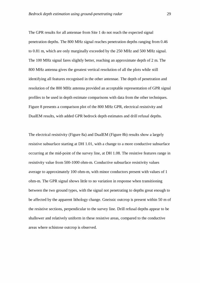
The GPR results for all antennae from Site 1 do not reach the expected signal
penetration depths. The 800 MHz signal reaches penetration depths ranging from 0.46
to 0.81 m, which are only marginally exceeded by the 250 MHz and 500 MHz signal.
The 100 MHz signal fares slightly better, reaching an approximate depth of 2 m. The
800 MHz antenna gives the greatest vertical resolution of all the plots while still
identifying all features recognised in the other antennae. The depth of penetration and
resolution of the 800 MHz antenna provided an acceptable representation of GPR signal
profiles to be used in depth estimate comparisons with data from the other techniques.
Figure 8 presents a comparison plot of the 800 MHz GPR, electrical resistivity and
DualEM results, with added GPR bedrock depth estimates and drill refusal depths.
The electrical resistivity (Figure 8a) and DualEM (Figure 8b) results show a largely
resistive subsurface starting at DH 1.01, with a change to a more conductive subsurface
occurring at the mid-point of the survey line, at DH 1.08. The resistive features range in
resistivity value from 500-1000 ohm-m. Conductive subsurface resistivity values
average to approximately 100 ohm-m, with minor conductors present with values of 1
ohm-m. The GPR signal shows little to no variation in response when transitioning
between the two ground types, with the signal not penetrating to depths great enough to
be affected by the apparent lithology change. Gneissic outcrop is present within 50 m of
the resistive sections, perpendicular to the survey line. Drill refusal depths appear to be
shallower and relatively uniform in these resistive areas, compared to the conductive
areas where schistose outcrop is observed.

Bedrock depth estimation using ground-penetrating radar 30
Fig
ure 8
: Com
pariso
n p
lot fo
r S
ite 1
show
ing: a
) electric
al r
esistiv
ity, b
) Du
alE
M a
nd
c) G
PR
resu
lts. Drill lo
ca
tion
s an
d d
ep
ths a
re m
ark
ed
on
all
plo
ts by b
lack
lines, w
ith d
ash
ed
bla
ck lin
es in
dica
ting d
rill dep
ths th
at e
xceed
the m
axim
um
dep
th o
f the p
lot. E
stimate
d G
PR
bed
rock
dep
th is
ma
rk
ed
on
the G
PR
ra
da
rgra
m, re
prese
nte
d b
y a
horiz
on
tal r
ed
line. P
lots a
re a
lign
ed
by d
rill hole c
oord
ina
tes. N
ote
tha
t the E
M a
nd
resistiv
ity
resu
lts are
to a
dep
th o
f 6 m
, com
pared
to G
PR
rad
argram
dep
th o
f ~2.6
metr
es.

Bedrock depth estimation using ground-penetrating radar 31
The 800 MHz GPR antenna bedrock depth estimates at each of the drill locations are
compared with the drill refusal depths at the same localities. A paired t-means test was
conducted to test the correlation between the two methods, the results of which are
presented in Table 3. The Pearson correlation value of -0.28 indicates no correlation
between the GPR estimates and drill refusal depths for the whole line (n = 13). Table 4
presents a second paired t-means test using GPR estimations and drill refusal depths
located within resistive areas (n = 4), giving a Pearson correlation of -0.95. The Pearson
correlation values suggest GPR bedrock depth estimates and drill refusal depths share
no correlation, regardless of subsurface conductivity conditions.
Table 3: Paired t-test to establish mean value and Pearson correlation between drill refusal depth
and GPR bedrock depth estimates at Site 1.
Table 4: Paired t-test to establish mean value and Pearson correlation between drill refusal depth
and GPR bedrock depth estimates at Site 1, using only data from locations in areas with large scale
resistive subsurface.
t-Test: Paired Two Sample for Means All Drill Holes
Drill GPR
Mean 2.096153846 0.609230769
Variance 0.997692308 0.012041026
Observations 13 13
Pearson Correlation -0.286284639
t-Test: Paired Two Sample for Means Resistive Areas
Drill GPR
Mean 1.6875 0.69
Variance 0.097291667 0.0178
Observations 4 4
Pearson Correlation -0.949181517

Bedrock depth estimation using ground-penetrating radar 32
5.2 Site 2: Chalkies Line
Figure 9 shows the depth of drill refusal along the transect from Site 2, relative to
surface elevation. The depth of refusal varies significantly over the traverse, ranging
from 0.60 m at DH 2.23, to a maximum of 7.30 m at DH 2.06. The drill tends to reach
greater depths in areas with flat topography, at the base of shallow inclines. An
exception to this is DH 2.10, which reaches a refusal depth of 5.20 m while being
located on a topographic high. Mean drill depth at the site is measured to be 2.81 m.
Field observations of nearby outcrop in the resistive areas found quartzite bedrock
exposed in close proximity to the survey line, along with large scale pegmatites
outcropping 50 m north of DH 2.08.
Figure 10 shows the plots of processed ground-penetrating radar data from the lowest
antennae frequency, 100 MHz (Figure 10a), to the largest, 800 MHz (Figure 10d),
across the Site 2 traverse. Moving from left to right, a small scale reflection is observed
at 60 m in the 250 MHz, 500 MHz and 800 MHz antennae. All three of the higher
frequency antennae detect a relatively high density of reflections from 120 to 200 m.
Figure 9: Cross-section of the Site 2 traverse. Drill hole locations and depths are marked relative
to regional topography.

Bedrock depth estimation using ground-penetrating radar 33
Fig
ure 1
0: C
om
parativ
e p
lot o
f processe
d g
rou
nd
-pen
etr
atin
g r
ad
ar d
ata
for S
ite 2 (C
ha
lkie
s Lin
e), sh
ow
ing; a
) 100
MH
z, b
) 25
0 M
Hz, c
) 500
MH
z a
nd
d) 8
00
MH
z an
ten
na re
sults. N
ote
that y
-axis d
ep
th is a
fun
ctio
n o
f sign
al v
elo
city
(m/n
s) an
d tim
e (ns). T
he tim
e w
ind
ow
s for ea
ch
an
ten
na
e (pre
sen
ted
in ta
ble
1) d
icta
te th
e m
axim
um
dep
th o
f wh
ich
da
ta c
an
be p
rese
nte
d fo
r ea
ch
an
ten
na
e.

Bedrock depth estimation using ground-penetrating radar 34
The 100 MHz antenna does not identify either of these reflectors. A small reflector is
recognised at approximately 180 m that is only detected by the 500 MHZ and 800 MHz
antennae. A small scale attenuation feature is seen by the 250 MHz and 800 MHz
antennae at 20-40 m. Signal penetration depth remains constant, only marginally
decreasing towards the end of the transect. The GPR results for all antennae from Site 2
do not reach the expected penetration depths. The 800 MHz signal reaches penetration
depths ranging from 0.48 to 1.03 m, which are only marginally exceeded by the
250 MHz and 500 MHz signals. The 100 MHz signal fares slightly better, reaching an
approximate depth of 2 m. The 800 MHz antenna gives the greatest vertical resolution
of all the plots while still identifying all features recognised in the other antennae. The
depth of penetration and resolution of the 800 MHz antenna provided an acceptable
representation of GPR signal profiles to be used in depth estimate comparisons with
data from other techniques. Figure 11 shows a comparison plot of the 800 MHz GPR,
electrical resistivity and DualEM results, with added GPR bedrock depth estimates and
drill refusal depths.
The electrical resistivity (Figure 11a) and DualEM (Figure 11b) results show a general
trend of conductive subsurface with a highly conductive lateral feature, reaching
resistivity values as low as 0.063 ohm-m, dominating from 2 to 4 m depth. This
conductive feature is present along most of the profile. A large scale highly resistive
body is detected in the central section of the traverse, starting 10 m east of DH 2.07, and
terminating 10 m west of DH 2.10. The lateral conductive feature does not occur within
the resistive body. Minor, shallow resistive bodies occur to the west of the central
resistive feature.

Bedrock depth estimation using ground-penetrating radar 35
Fig
ure 1
1: C
om
pariso
n p
lot fo
r S
ite 2
, show
ing: a
) ele
ctr
ica
l resistiv
ity, b
) Du
alE
M a
nd
c) G
PR
resu
lts. Drill lo
catio
ns a
nd
dep
ths a
re m
ark
ed
on
all p
lots
by b
lack
lines, w
ith d
ash
ed
bla
ck lin
es in
dica
ting d
rill dep
ths th
at e
xceed
the m
axim
um
dep
th o
f the p
lot. E
stimate
d G
PR
bed
rock
dep
th is m
ark
ed
on
the
GP
R r
ad
argra
m, r
ep
rese
nte
d b
y a
horiz
on
tal r
ed
line. P
lots a
re a
lign
ed
by d
rill hole c
oord
ina
tes. N
ote
tha
t the E
M a
nd
resistiv
ity re
sults a
re to
a d
ep
th o
f
6 m
, com
pared
to G
PR
rad
arg
ram
dep
th o
f ~2.6
metr
es.

Bedrock depth estimation using ground-penetrating radar 36
The resistive bodies have values ranging from 1000 – 10 000 ohm-m. DH 2.01- 2.05,
DH 2.12 and DH 2.13 hit refusal at first contact with the conductive feature. The
resistive areas correspond with areas of increased penetration depth in the processed
GPR data, and hyperbola in the raw GPR data (see Appendix D). The GPR signal
outside of the resistive sections show minor reflections, with extended sections showing
zero reflections and complete signal attenuation. Shallow drill refusal corresponds with
resistive subsurface at DH 2.08, DH 2.09 and DH 2.11.
The bedrock depth estimates provided by the 800 MHz GPR antenna at each of the drill
locations were compared with the drill refusal depths at the same localities. A paired t
means test was conducted to test the correlation between the two methods, the results of
which are presented in Table 5. A second paired t means test was conducted using drill
refusal and GPR bedrock depth estimate data collected at DH 2.08, DH 2.09, DH 2.10
and DH 2.11, which are all located within resistive bodies identified in Figures 11a and
11b. The results of the second paired t means test are presented in Table 6. In the
resistive areas the Pearson correlation value is 0.97, showing a strong correlation
between GPR depth estimates and drill refusal depths . These results use a small sample
size (n = 4) due to the low drill count through the resistive bodies. The Pearson
correlation value over the entire survey line (n = 22) is -0.17, showing no correlation
between the GPR and drill refusal depths.
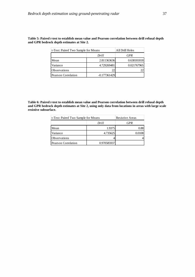
Bedrock depth estimation using ground-penetrating radar 37
Table 5: Paired t-test to establish mean value and Pearson correlation between drill refusal depth
and GPR bedrock depth estimates at Site 2.
Table 6: Paired t-test to establish mean value and Pearson correlation between drill refusal depth
and GPR bedrock depth estimates at Site 2, using only data from locations in areas with large scale
resistive subsurface.
t-Test: Paired Two Sample for Means All Drill Holes
Drill GPR
Mean 2.811363636 0.638181818
Variance 4.729269481 0.021767965
Observations 22 22
Pearson Correlation -0.177361429
t-Test: Paired Two Sample for Means Resistive Areas
Drill GPR
Mean 1.9375 0.88
Variance 4.735625 0.0108
Observations 4 4
Pearson Correlation 0.970585937

Bedrock depth estimation using ground-penetrating radar 38
5.3 Site 3: Canham Road
Figure 12 shows the depths of drill refusal along the transect from Site 3, relative to
surface elevation. The depth of refusal varies from 0.40 m at DH 3.23 to a maximum of
6.80 m at DH 3.16, with a mean depth of 2.38 m. Refusal depths tend to increase at
lower elevations, with the deepest refusal point (DH 2.16) located at a topographic low.
Refusal depth is significantly shallower at topographic highs, where abundance of loose
quartzite and iron stones are present, suggesting a change to the soil profile relative to
topography.
Figure 13 shows the plots of processed ground-penetrating radar data from the lowest
antennae frequency, 100 MHz (Figure 13a), to the highest, 800 MHz (Figure 13d),
across the traverse ate Site 3.
Figure 12: Cross-section of the Site 3 traverse. Drill hole locations and depths are marked relative
to regional topography.

Bedrock depth estimation using ground-penetrating radar 39
Fig
ure 1
3: C
om
pa
riso
n p
lot o
f processe
d g
rou
nd
-pen
etr
atin
g r
ad
ar d
ata
for S
ite 3 (C
an
ha
m R
oa
d), sh
ow
ing
; a) 1
00 M
Hz, b
) 25
0 M
Hz,
c) 5
00
MH
z an
d d
) 800 M
Hz a
nte
nn
a r
esu
lts. Note th
at y
-axis d
ep
th is a
fun
ctio
n o
f sign
al v
elo
city
(m/n
s) an
d tim
e (ns). T
he tim
e
win
dow
s for e
ach
an
ten
nae (p
rese
nte
d in
tab
le 1) d
icta
te the m
axim
um
dep
th o
f wh
ich
data
ca
n b
e pre
sen
ted
for ea
ch
an
ten
nae.

Bedrock depth estimation using ground-penetrating radar 40
The GPR estimates from each of the antenna generally show similar patterns regarding
reflection locations and penetration depths. Reflectors are detected on all antennae from
0 to 100 m. Higher frequency antennae detect these reflectors further along the profile
than lower frequency antennae. Excluding a small scale reflector at 280 meters, no
notable reflections are present for all antennae along the rest of the transect. The 500
MHz and 800 MHz antennae show the strongest correlation to one another. The GPR
results for all antennae from Site 3 do not reach expected penetration depths. The 800
MHz signal reaches penetration depths ranging from 0.40 to 0.89 m, which are only
marginally exceeded by the 250 MHz and 500 MHz antennae. The 100 MHz signal
fares slightly better, reaching an approximate depth of 2 m. Due to the limited
penetration of depth all antennae, the ability of the 800 MHz antenna to show greater
resolution resulted in it being chosen to be further analysed and compared to other
geophysical and drilling data sets. The 800 MHz antenna data is presented in a
comparative plot with electrical resistivity and DualEM data in Figure 14.
The electrical resistivity (Figure 14a) and DualEM (Figure 14b) results show a general
trend of conductive subsurface with minor variations at depth in areas of low
topographic relief. A large resistor is present from 15 m east of DH 3.01, to DH 3.06
which among the highest elevation points of the transect. At DH 3.06 there is a contact
between the resistive feature and a more conductive part of the section which dominates
for the rest of the profile. Shallow resistors are present between DH 3.10 to DH 3.13
and DH 3.16 – DH 3.17. Resistivity readings are typically within 100 – 1000 ohm-m,
with highly resistive areas reaching up to 10 000 ohm-m.

Bedrock depth estimation using ground-penetrating radar 41
Fig
ure 1
4: C
om
pariso
n p
lot fo
r S
ite 3
, show
ing
: a) e
lectr
ica
l resistiv
ity, b
) Du
alE
M a
nd
c) G
PR
resu
lts. Drill lo
ca
tion
s an
d
dep
ths a
re m
ark
ed
on
all p
lots b
y b
lack
lines, w
ith d
ash
ed b
lack
lines in
dica
ting d
rill d
ep
ths th
at e
xceed
the m
axim
um
dep
th o
f
the p
lot. E
stimate
d G
PR
bed
rock
dep
th is m
ark
ed
on
the G
PR
ra
dargra
m, r
ep
rese
nte
d b
y a
horiz
on
tal r
ed
line. P
lots a
re
alig
ned
by d
rill h
ole
coord
inate
s. Note th
at th
e EM
an
d re
sistivity
resu
lts are to
a d
ep
th o
f 6 m
, com
pared
to G
PR
rad
argram
dep
th o
f ~2.6
metr
es.

Bedrock depth estimation using ground-penetrating radar 42
The observed conductive areas rarely reach values below 1 ohm-m. The change from
resistive to conductive subsurface has a notable effect on drill refusal depths, as all
observed refusal depths below 1 m occurs within resistive areas. These resistive areas
also correspond with areas of increased signal penetration depth and reflections in the
processed GPR data. The GPR signal outside of the resistive sections shows minor
reflections, with extended sections showing zero reflections and complete signal
attenuation.
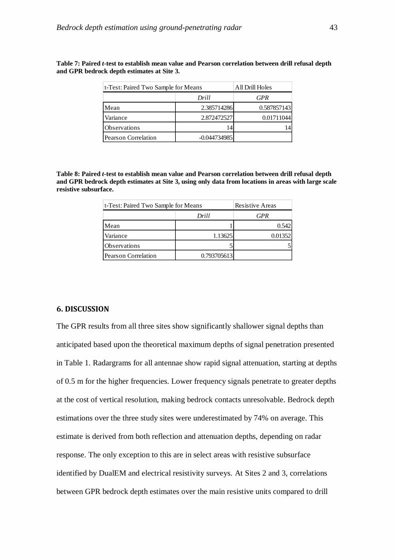
The bedrock depth estimates provided by the 800 MHz GPR antenna at each of the drill
locations were compared with the drill refusal depths at the same localities. A paired t
means test was conducted to test the correlation between the two methods, the results of
which are presented in Table 7. A second paired t means test was conducted using drill
refusal and GPR bedrock depth estimate data collected at DH 2.08, DH 2.09, DH 2.10
and DH 2.11, which are all located within resistive bodies identified in Figure 14.
The results of the second paired t means test are presented in Table 8. In the resistive
areas the Pearson correlation value is 0.97 which shows a strong correlation between
GPR depth estimates and drill refusal results. These results use a small sample size
(n = 4) due to the low drill count through the resistive bodies. The Pearson correlation
value over the entire survey line (n = 14) is -0.17, showing no correlation between the
GPR and drill refusal depths.
Bedrock depth estimation using ground-penetrating radar 43
Table 7: Paired t-test to establish mean value and Pearson correlation between drill refusal depth
and GPR bedrock depth estimates at Site 3.
Table 8: Paired t-test to establish mean value and Pearson correlation between drill refusal depth
and GPR bedrock depth estimates at Site 3, using only data from locations in areas with large scale
resistive subsurface.
6. DISCUSSION
The GPR results from all three sites show significantly shallower signal depths than
anticipated based upon the theoretical maximum depths of signal penetration presented
in Table 1. Radargrams for all antennae show rapid signal attenuation, starting at depths
of 0.5 m for the higher frequencies. Lower frequency signals penetrate to greater depths
at the cost of vertical resolution, making bedrock contacts unresolvable. Bedrock depth
estimations over the three study sites were underestimated by 74% on average. This
estimate is derived from both reflection and attenuation depths, depending on radar
response. The only exception to this are in select areas with resistive subsurface
identified by DualEM and electrical resistivity surveys. At Sites 2 and 3, correlations
between GPR bedrock depth estimates over the main resistive units compared to drill
t-Test: Paired Two Sample for Means All Drill Holes
Drill GPR
Mean 2.385714286 0.587857143
Variance 2.872472527 0.01711044
Observations 14 14
Pearson Correlation -0.044734985
t-Test: Paired Two Sample for Means Resistive Areas
Drill GPR
Mean 1 0.542
Variance 1.13625 0.01352
Observations 5 5
Pearson Correlation 0.793705613

Bedrock depth estimation using ground-penetrating radar 44
refusal depths were notably improved. The r2 values at these sites are 0.94 and 0.63
respectively, showing moderate to strong linear trends for GPR depth estimations and
drill refusal depths. The resistive areas identified at Site 1 did not prove to influence
radar signal in any way. The resistors at this site (~500-1000 ohm-m), are notably less
resistive than the resistive zones highlighted at Sites 2 and 3 (~1000-10000 ohm-m).
This is an interesting feature of the site that requires further field evaluation.
The electrical resistivity and DualEM results displayed a strong correlation with depth
to drill refusal and the top of highly conductive bodies. Most drill holes at Site 2 show
refusal at a lateral conductive feature that occurs at 2-4 m depth. Interestingly, some of
the drill holes appear to have encountered localised areas where this conductive unit
was not as hard and the drill was able to penetrate to greater depths. This is interpreted
as a localised change in the geology that is not resolvable with any of the geophysical
techniques used. A similar trend is observed at Site 3, where drilling in areas
determined by electrical resistivity and DualEM to be highly resistive resulted in refusal
depths less than 1 m. Nearby drill holes in conductive areas reached depths of up to 4.7
m at this site. This ambiguity reflects the likelihood that the contacts between overlying
soils and bedrock are often not sharp, defined boundaries. Products of bedrock called
saprolite form as the bedrock is weathered by chemical and mechanical means. This
saprolite forms a fragmented, weathered layer of variable thickness atop of the
unweathered bedrock (McDonald & Isbell 2009). The type of bedrock and associated
weathering index control the thickness of this saprolitic rock layer (Curmi et al. 1994).
Materials resistive to chemical weathering, such as quartzite, tend to have thin saprolite
layers, while materials more susceptible to chemical weathering tend to have thicker

Bedrock depth estimation using ground-penetrating radar 45
saprolite layers (Curmi et al. 1994). The push-tube percussion drill used for this study is
not designed to core through this moderately weathered bedrock (M. Thomas pers.
comm. 2013); potentially resulting in imprecise ground truthing data.
6.1 GPR Signal Attenuation
GPR signal attenuation was observed in the radargrams for all antennae frequencies at
each site. Olhoeft (1986) identifies signal scattering, soil conductivity and clay content
to attribute to GPR signal attenuation. Work by Van Dam et al. (2002) and Josh et al.
(2011) also identify the iron oxide content within soils to also have a profound impact
on signal attenuation. These four factors are discussed, relative to the survey results.
6.1.1 SIGNAL SCATTERING
Under favourable conditions GPR surveying has the potential to identify coarse rock
fragments (Sucre et al. 2010). High concentrations of irregularly shaped coarse
fragments can cause signal loss by unpredictable redirection of GPR signal away from
the receiver antenna. This type of scattering is common if the incident wavelength is 3 -
10 times smaller than the object. Higher frequency antennae, such as the 500 MHz and
800 MHz used in this study, are more susceptible to signal scattering than lower
frequency antennae (Reynolds 1997). Large, coarse fragments that resemble bedrock are
more extensive in more developed and extensively weathered profiles. The 100 MHz
and 250 MHz antennae showed no increase in reflections where higher frequency
antennae show loss of signal. Thus, it is unlikely that signal scattering contributed to the
GPR signal attenuation.

Bedrock depth estimation using ground-penetrating radar 46
6.1.2 SOIL CONDUCTIVITY
The attenuation factor of radar signal, presented in Equations 5 and 6, indicate the main
influences of signal attenuation in low-loss soil to be the bulk conductivity and
dielectric constant (Reynolds 1997). The loss tangent (P) of the soil increases as a
function of a materials conductivity (see Equation 2). Features with high conductivity
attributes (i.e. lossy soil) cause electromagnetic signal to be converted into thermal
energy, which the GPR can no longer measure (Olhoeft 1986). The increase in signal
quality within the resistive sections at Sites 2 and 3 suggests that terrain conductivity is
attributing to the attenuation of GPR signal. The exception to this is Site 1, in which
signal attenuation is observed to have no correlation to conductive areas. The resistors
observed at Site 1 are a factor of 10 less resistive than those seen at Site 2 and 3. It is
worth nothing that resistivity values at very shallow depths cannot be accurately
obtained using the applied EM and electrical resistivity techniques, due to skin depth
and resolution factors (Fitterman & Labson 2005). Du and Rummel (1994) found low
frequency antennae to be affected by conductive soil conditions to a greater degree than
higher frequency antennae. Over all three sites the 100 MHz signal averages a
penetration depth of approximately 2 m, instead of the theoretical 10.18 m, showing an
81% underestimation of signal penetration. The antenna shows poor vertical and
horizontal resolution at all three sites, with most features rendered undefinable. In
comparison the 800 MHz antenna reaches approximately 0.8 m, instead of the
theoretical 2.05 m, showing a loss of 61%. This antenna displays high vertical
resolution, but still poor horizontal resolution. The poor horizontal resolution suggests
that the soil at all three sites are unlikely to be low-loss geological materials for the
antennae frequencies used in the survey (Hatch et al. 2013). The observed resistivity

Bedrock depth estimation using ground-penetrating radar 47
values for the conductive areas at the surface are considered to not be low enough to
cause the degree of signal attenuation observed at each site. This suggests that while soil
conductivity could be a major factor causing signal attenuation, other factors that
influence the dielectric constant of the soil, such as moisture, clay content and iron
oxide content could be the primary cause of signal attenuation seen across the sites.
6.1.3 CLAY CONTENT
According to Reynolds (1997), the soil velocity (v = 0.14m/ns) is indicative of dry sand
(0.12 - 0.17 m/ns) and between wet (86 - 110 m/ns) to dry (173 m/ns) clay. Examination
of the soil samples collected at each site shows that the soil profile tends to have dry
topsoil; with moisture contents increasing at depths ranging from 0.3 to 0.9 m. These
values suggest that signal initially passes through dry sandy soil horizon. The signal
then contacts a layer between 0.30 - 0.60 m depth, with a twofold increase in moisture
content than that of the dry sand. These depths correspond with observed A and B
horizon depths (see Appendix B). The velocity of this layer lies between standard
velocities for saturated to dry clay (Reynolds 1997). The presence of clays, particularly
with saline groundwater, increases signal attenuation and decreases signal velocity by
increasing a soils dielectric constant and bulk conductivity (Doolittle et al. 1994,
Reynolds 1997). Clays exhibit distinct electrical properties due to their physiochemical
structure which includes bound water within its lattice (Reynolds 1997). Clays are also
mineralogically unique as they consist of colloidal particles which have an uneven
distribution of charge (Olhoeft 1986, Reynolds 1997). Positive charges accumulate
within the lattice structure of the clay, while negative charges accumulate on the clays
exterior (Olhoeft 1986). The application of an EM field via GPR signal causes the

Bedrock depth estimation using ground-penetrating radar 48
charge on the clay particles to migrate, converting kinetic energy to thermal energy
(Olhoeft 1986). Thermal energy is undetectable by the GPR signal and signal will
appear attenuated on a GPR record (Reynolds 1997). Clay-rich, highly conductive soils
will yield signal penetration depths of less than 1 m for frequencies as low as 100 MHz
(Wright et al. 1984). These shallow penetration depths were observed at all three study
sites. The presence of clay and increased moisture content at depth observed at each site
provides an explanation of the attenuation of GPR signal. Further work to quantify the
clay content of the soils needs to be conducted before the overall effect of this factor can
be determined.
6.1.4 IRON OXIDE CONTENT
Van Dam et al. (2002) demonstrated that the presence of iron oxide as precipitates does
not directly influence the three components of electromagnetic waves (µ, σ and ε).
Thus, the concentration of iron oxide does not alter the relative dielectric permittivity of
a sediments solid phase (Mätzler 1998). Iron oxides only have an influence on the
dielectric permittivity of a soil when water is present (Van Dam et al. 2002). The
amount of iron oxide present within a material correlates to volumetric water content
(Van Dam et al. 2002). This correlation is caused by the capillary retention capacity of
iron oxides compared to other minerals. As previously discussed, the soil moisture
content of the soils at each site increased with depth. This increase has the potential to
correlate to increased dissolved iron oxides within the soil profiles, contributing to
signal attenuation. Josh et al. (2011) discovered iron oxide concentrations of 0.4% wt.
within favourable GPR survey conditions to reduce 250 MHz signal penetration depth
from 10 m to below 1 m. The iron oxide minerals in this study occurred within a clay
Bedrock depth estimation using ground-penetrating radar 49
coating on quartz grains, along with subsidiary amounts of kaolin, carbonates and
smectite (Josh et al. 2011). It is worth noting that the soils observed at Site 3 were
logged as ferruginous due to their red hue, while soils at Sites 1 and 2 not displaying
this feature. Without quantifying if dissolved iron oxide occurred in the horizons, or as
inclusions within clay coatings on grains, the exact influence of iron oxides on the
dielectric properties of the soils at the study sites, if any, cannot be identified. Thus, the
role of iron oxides as a contributor to the observed signal attenuation cannot be
determined.
6.2 Signal attenuation summary
Considering all these factors, it is determined that signal scatter is unlikely to have
occurred at any of the sites. The cause of attenuation has been narrowed to ground
conductivity, clay content and iron oxide presence. These factors all tend to have an
increased chance of occurring within a soils B horizon (Doolittle & Collins 1995). The
average B horizon ranges at each site are as follows: Site 1 ≅ 0.36 - 0.91 m depth, Site 2
≅0.23 - 0.85 m depth and Site 3 ≅ 0.18 - 1.30 m depth. The B horizon was present
throughout Site 1, with subsurface conductivity sharing no relation to thickness of the
horizon. Site 2 and 3 demonstrated the thickness of the B horizon to be negatively
influenced by the presence of resistive subsurface features. The B horizon was on
average between 0.0 – 0.15 m thick in areas where resistors were present. GPR signal in
these areas penetrated to greater depths and provided more accurate bedrock depth
estimates when compared to drilling results. The direct correlation between B horizon
presence and signal attenuation at all three sites could be attributed to conductive, lossy
soil conditions with increased iron oxide and clay presence in the B horizon amplifying
Bedrock depth estimation using ground-penetrating radar 50
signal attenuation. Without further in-depth analysis of these factors, it is difficult to
make a solid conclusion regarding the primary cause of this signal attenuation.
7. CONCLUSIONS
The type of terrain in which data are collected is highly influential to the practical
applicability of GPR, with soil type, moisture and conductivity all having potentially
severe impacts on the quality of collected data. In the instance of Adelaide Hills-type
soils found at Mount Crawford, this study has shown GPR to be relatively ineffective.
Signal attenuation greatly affected the signal penetration depth and clarity at all three
sights. The cause of attenuation is speculated to be caused by the clay contents, iron
oxide contents and bulk conductivities of the investigated soils. These factors typically
increase in value within B horizon soils, in which all observed signal attenuation
occurred. It is likely that a combination of all three of the above factors caused the
signal loss. The system showed increased estimation accuracy in areas with highly
resistive subsurface detected by electrical resistivity and EM surveys; though sample
sizes in these areas were small, and the results were not consistent across all three sites.
The tendency of weathered terrains to have more developed B horizons leads to the
recommendation of using other geophysical methods, such as electrical resistivity, in
Adelaide Hills-type environments. An explicit knowledge of the soil properties in the
target terrain is advantageous, thus local soil studies should be considered in these types
of environments before the application of a GPR survey.
Bedrock depth estimation using ground-penetrating radar 51
8. ACKNOWLEDGMENTS
I would like to thank Michael Hatch for his constant support, comments and role as
project supervisor throughout the year. I would also like to thank Mark Thomas and
John Wilford from the CSIRO and Geoscience Australia for research funding and
support. I would like to thank John Triantafilis and Thomas Fotheringham for data
collection assistance, processing EM and resistivity data, and providing valuable
comments. Thanks to David Hamilton-Smith, Kate Robinson and Sebastian Schnaidt
for assistance in the field. Thanks to Jingping Zhe, Phil Mill, and Mads Toft for
assistance with processing software. Thanks also to Katie Howard for organising project
deadlines and support throughout the year. Finally, thanks to Lars Krieger for help with
thesis drafting and editing.
9. REFERENCES
ANNAN A. P. 2005. Ground-Penetrating Radar. In: Butler D. K. ed., Near-Surface Geophysics, Vol. Investigations in Geophysics, pp 357-438, Society of Exploration Geophysicists.
BANTON O., SEGUIN M. K. & CIMON M. A. 1997. Mapping field scale physical properties of soil with electrical resistivity. Soil Sci. Soc. Am. J. 61, 1010-1017.
BENBOW M. C., ALLEY N. F., CALLEN R. A. & GREENWOOD D. R. 1995. Geological history and palaeoclimate. In: Drexel J. F. & Preiss W. V. eds., The geology of South Australia, Vol. 54, pp 208-217, Geological Survey of South Australia Bulletin.
BLACKBURN G. 1958. Soil Mapping in the Mt. Crawford Forest Reserve, South Australia. Technical Memo. CSIRO Division of Soils.
BOURMAN R. P. & LINDSAY J. M. 1989. Timing, extent and characted of Late Cainozoic Faulting on the eastern margin of the Mt Lofty Ranges, South Australia. 113: 63-67. Royal Society of South Australia.
CAI J. & MCMECHAN G. A. 1995. Ray-based synthesis of bistatic ground-penetrating radar profiles. Geophysics 60, 87-96.
CARCIONE J. M. 1996. Ground-penetrating radar: wave theory and numerical simulation in lossy anisotropic media. Geophysics 61, 1664-1677.
CHANZY A., TARUSSOV A., JUDGE A. & BONN F. 1996. Soil water content determination using a digital ground-penetrating radar. Soil Sci. Soc. Am. J. 60, 1318-1326.
CHARLTON M. B. 2008. Principles of ground-penetrating radar for soil moisture assessment. Walker institute for Climate System Research, University of Reading.
COLLINS M. E. & DOOLITTLE J. A. 1987. Using ground penetrating radar to study soil microvariability. Soil Sci. Soc. Am. J. 51, 491-493.
CONOR C. H. H. 1984. Draft report, Williamstown industrial mineral deposits. Geology of koalin-sillimanite-muscovite deposits, near Williamstown, Hd. Barossa, Mt. Lofty Ranges, South Aust. Department of Primiary Industries and Resources South Australia Report Book 84/65.
COULOUMA G., SAMYN K., GRANDJEAN G., FOLLAIN S. & LAGACHERIE P. 2011. Combining seismic and electric methods for predicting bedrock depth along a Mediterranean soil toposequence. Geoderma 170, 39-47.

Bedrock depth estimation using ground-penetrating radar 52
COULOUMA G., TISSEYRE B. & LAGACHERIE P. 2010. Is a Systematic Two-Dimensional EMI Soil Survey Always Relevant for Vineyard Production Management? A Test on Two Pedologically Contrasting Medieterranean Vineyards. In: Viscarra Rossel R. A., McBratney A. & Minasny B. eds., Proximal Soil Sensing. Progress in Soil Science series, pp 283-295, Springer, New York.
CURMI P., WIDIATMAKA, PELLERIN J. & RUELLAN 1994. Saprolite influence on formation of well-drained hydromorphic horizons in an acid soil system as determined by structural analysis. Developments in Soil Science 22, 133-140.
DAILY B., FIRMAN J. B., FORBES B. G. & LINDSAY J. M. 1976. Geology. In: Twidale C. R. T., Tyler M. J. & Webb B. P. eds., Natural History of the Adelaide Region, Royal society of South Australia Inc.
DAVIS J. L. & ANNAN A. P. 1989. Ground-penetrating radar for high-resolution mapping of soil and rock stratigraphy. Geophysical Prospecting 37, 531-551.
DOOLITTLE J. A. & COLLINS M. E. 1995. Use of soil information to determine application of ground penetrating radar. Journal of Applied Geophysics 33, 101-108.
DOOLITTLE J. A., SUDDUTH K. A., KITCHEN N. R. & INDORANTE S. J. 1994. Estimating depths to claypans using electromagnetic induction methods. J. Soil and Water Cons 49, 572-575.
DU S. & RUMMEL P. 1994. Reconnassance studies of moisture in the subsurface with GPR. Proceedings of the Fifth International Conference on Ground Penetrating Radar, Kitchener, Ontario, pp. 1241-1248.
FITTERMAN D. V. & LABSON V. F. 2005. Electromagnetic Induction Methods for Environmental Problems. In: Butler D. K. ed., Near-Surface Geophysics, Vol. Investigations in Geophysics, pp 301-356, Society of Exploration Geophysicists.
FITZPATRICK E. A. 1988. Soil Horizon Designation and Classification. International Soil Reference and Information Centre.
FORESTRYSA 2006. Little Mount Crawford Native Forest Reserve Management Plan. Forestry SA.
GEONICS LIMITED 2013. DUALEM-421s User Guide. GRIFFIN S. & PIPPET T. 2002. Ground Penetrating Radar. CRCLEME Open File Report
Geophysical and Remote Sensing Methods for Regolith Exploration. HATCH M., HEINSON G., MUNDAY T., THIEL S., LAWRIE K., CLARKE J. D. A. & MILL P. 2013.
The importance of including conductivity and dielectric permittivity information when processing low-frequency GPR and high-frequency EMI data sets. Journal of Applied Geophysics 96, 77-86.
JACKSON E. A. 1957. A survey of the soils and their utilisation in portion of the Mt. Lofty Ranges, South Australia. Soils and Land Use Service. 21. CSIRO Division of Soils.
JOL H. M. & BRISTOW C. S. 2003. An introduction to ground penetrating radar (GPR) in sediments. In, Ground penetrating radar in sediments, Vol. 211, pp 1-7, Geological Society Special Publications, London.
JOL H. M. & SMITH D. G. 1991. Ground penetrating radar of northern lacustrine deltas. Can. J. Earth Sci. 28, 1939-1947.

Bedrock depth estimation using ground-penetrating radar 53
JOSH M., LINTERN M. J., KEPIC A. W. & VERRAL M. 2011. Impact of grain-coating iron minerals on dielectric response of quartz sand and implications for ground-penetrating radar. Geophysics 76, J27-J34.
KEAREY P., BROOKS M. & HILL I. 2002. An introduction to geophysical exploration. Blackwell Science.
MALA GEOSCIENCE 2013. X3M control unit user manual. MÄTZLER C. 1998. Microwave permittivity of dry sand. IEEE Trans. Geosci. Remote
Sensing 36, 317-319. MCDONALD R. C. & ISBELL R. F. 2009. Soil Profile. In, Australian Soil and Land Survey
Field Handbook, pp 147-200, CSIRO, Melbourne. MCNEILL J. D. 1990. Use of Electromagnetic Methods for Groundwater Studies. In:
Ward S. H. ed., Geotechnican and Environmental Geophysics, Vol. Volume 1: Review and Tutorial, Anacortes, Washington, US.
MCNIELL J. D. 1980. Applications of Transient Electromagnetic Techniques. Geonics Limited.
MONTEIRO SANTOS F. A., TRIANTAFILIS J., BRUZGULIS K. E. & ROE J. A. E. 2009. Inversion of DUALEM-421 profiling data using a 1-D laterally constrained algorithm. Vadose Zone Journal 9, 117-125.
OLHOEFT G. R. 1986. Direct detection of hydrocarbon and organic chemicals with ground penetrating radar and complex resistivity. NWWA/API Conference on Petroleum, Hydrocarbons and Organic Chemicals in Ground Water - Prevention, Detection and Restoration.
PREISS W. V. 1987. Basement inliers of the Mount Lofty Ranges. In, The geology of South Australia, Volume 1, The Precambrian, pp 102-105, Geological Survey of South Australia, Adelaide.
PREISS W. V., FANNING C. M., SAPUNAR M. A. & BURTT A. C. 2008. Age and tectonic significance of the Mount Crawford Granite Gneiss and a related intrusive in the Oakbank Inlier, Mount Loft Ranges, South Australia. MESA Journal 49, 38-40.
REYNOLDS J. M. 1997. An Introduction to Applied and Environmental Geophysics. Wiley, Chichester.
SAARENKETO T. 1998. Electrical properties of water in clay and silty soils. J. Appl. Geophys. 40, 73-88.
SAMOUELIAN A., COUSIN I., TABBAGH A., BRUAND A. & RICHARD G. 2004. Electrical resistivity survey in soil science: a review. Soil & Tillage Research 83, 173-193.
SANDIFORD M. 2002. Neotectonics of southeastern Australia: linking the Quaternary faulting record with seismicity and in situ stress. Geological Society of Australia Special Publication 22.
SUCRE E. B., TUTTLE J. W. & FOX T. R. 2010. The use of ground-penetrating radar to accurately estimate soil depth in rocky forest soils. Forest Science 57, 59-66.
TELFORD W. M., GELDART L. P., SHERIFF R. E. & KEYS D. A. 1990. Applied Geophysics (2nd edition). Cambridge University Press, Cambridge.
TOKAREV V. 2005. Neotectonics of the Mount Lofty Ranges (South Australia). PhD thesis, School of Earth & Environmental Sciences, Geology & Geophysics, The University of Adelaide, Adelaide (unpubl.).

Bedrock depth estimation using ground-penetrating radar 54
TOKAREV V. & GOSTIN V. 2003. Mt Lofty Ranges, South Australia. Regolith-Landscape Evolution Across Australia. Anand R. R. & De Broekert P. Cooperative Research Center for Landscape Evolution and Mineral Exploriation, Canberra.
TOWNSEND I. J. 1984. Williamstown clay mine, a unique deposit? South Australia Department of Mines and Energy South Australia - Exploration Potential.
TRIANTAFILIS J. & BUCHANAN S. M. 2009. Identifying common near-surface and subsurface stratigraphic units using EM34 signal data and fuzzy k-means analysis in the Darling River valley. Australian Journal of Earth Sciences 56, 535-558.
TRIANTAFILIS J., TERHUNE IV C. H. & MONTEIRO SANTOS F. A. 2013. An inversion approach to generate electromagnetic conductivity images from signal data. Environmental Modelling and Software 43, 88-95.
VAN DAM R. L., SCHLAGER W., DEKKERS M. J. & HUISMAN J. A. 2002. Iron oxides as a cause of GPR reflections. Geophysics 67, 536-545.
WIGHTMAN W. E., MARTINEK B. C. & HAMMERMEISTER D. 1992. Geophysical Methods Used to Guide Hydrogeological Investigations at an Umtra Site Near Grand Junction, Colorado. In: Nielsen D. M. & Sara M. N. eds., Current Practices in Ground Water and Vadose Zone Investigations, American Society for testing and Materials, Philadelphia.
WILFORD J. & THOMAS M. 2012. Modelling soil-regolith thickness in complex weathered landscapes of the central Mt Lofty Ranges, South Australia. Digital Soil Assessments and Beyond, Sydney, Australia, pp. 69-75. Taylor and Francis Group.
WRIGHT D. L., OLHOEFT G. R. & WATTS R. D. 1984. Ground-penetrating radar studies on Cape Cod. In: Nielsen D. M. ed., Surface and borehole geophysical methods in groundwater investigations, pp 666-680, Nat. Water Well Assoc., Worthington, OH.
ZHE J., GREENHALGH S. A. & MARESCOT L. 2007. Multichannel, full waveform and flexible electrode combination resistivity-imaging system. Geophysics 72, 57-64.
ZHOU B. & GREENHALGH S. A. 1999. Explixit expressions and numerical calculations for the Frechet and second derivatives in 2.5D Helmholtz equation inversion. Geophysical Prospecting 47, 443-468.
ZONGE K., WYNN J. & URQUHART S. 2005. Resistivity, Induced Polarization and Complex Resistivity. In: Butler D. K. ed., Near-Surface Geophysics, Vol. Investigations in Geophysics, pp 265-300, Society of Exploration Geophysicists.
Bedrock depth estimation using ground-penetrating radar 55
APPENDIX A:
DETAILED METHODS

Bedrock depth estimation using ground-penetrating radar 56
Ground Penetrating Radar
Equipment/application: A MALÅ geoscience X3M GPR control unit and MALÅ XV
monitor was used with 100 MHz, 250 MHz, 500 MHz and 800 MHz fixed-separation
shielded antennae, mounted on a rough terrain push cart. The traverses at each site were
based upon the drilling locations, with the GPR track passing approximately 20cm to
the right of each of the drill holes. At each site the required settings for the antennae
were set as observed in Table 1. Data were collected a total of 4 times at each site per
antennae.
Table 1: GPR settings
The traverses using the GPR were made travelling in forward and reverse directions
twice, giving a total of 4 traverse files to be used for analysis. All GPR data have been
taken assuming vertical incidence due to the small antennae spacings. A differential
GPS was attached to the GPR system allowing coordinates to be recorded into the data
file.
Processing: The raw data were imported and processed as follows:
1) Raw data file imported into Reflex W using RAMAC GPR settings
2) Raw data associated with .COR file containing GPS coordinates
3) Coordinates converted to WGS 84 zone54s
4) Subtract mean (DeWow) 1D filter removed any DC offset
5) Static correction by manual picking of the first positive phase arrival to remove air
wave.
6) Background removal filter was applied to remove all background noise and present
a truer signal
7) Wave velocity determined by hyperbola reflection analysis, giving a depth function
of 0.14 m/ns
8) F-K migration (Stolt) was applied using a velocity function of 0.14 m/ns to reduce
hyperbola presence and present a truer image of subsurface features
9) Enveloping of the signal, converting negative phase data into a positive phase
10) 2D running average filter applied to each transect acted as a smoothing filter for
final presentation and result interpretation. Traces averages used for each antenna
Antennae 100 MHz 250 MHz 500 MHz 800 MHz
Time Window 198.6 ns 140.0 ns 78.8 ns 39.6 ns
Theoretical Max Depth
10.18 m 7.18 m 4.03 m 2.05 m
Point/Time Interval
0.25 s 0.05 m 0.04 m 0.019 m
Samples Per Interval
344 536 624 512
Sampling Frequency
1581.25 MHz 3614.29 MHz 7535.71 MHz 12173.08MHz
Antennae fixed offset
0.5 m 0.36 m 0.18 m 0.14 m

Bedrock depth estimation using ground-penetrating radar 57
were as follows: 100 MHz – 5 traces, 250 MHz – 10 traces, 500 MHz – 20 traces,
800 MHz – 40 traces.
The below figure presents a typical processing flow from a fully filtered data set.
Full detailed explanations of the applications for each filtering step are available in the
ReflexW user guide. Note that gain functions were not applied to any data sets as many
became distorted, even at low decibel increases.
Following processing, location and depth of each drill hole was manually picked based
upon the GPS coordinates. Bedrock depth estimations were made using a phase
follower picking method with a tolerance of +0.25 amplitude. This was initially picked
manually in resistive zones where bedrock depth estimations were most accurate. The
phase follower automatically picked the remained of the data and created a bedrock
estimate layer. This layer was viewed manually to determine if the picks corresponded
to bedrock reflections, or to signal attenuation. Visual analysis of each antennae
established the frequency that produced the most accurate bedrock estimates.
Data were exported into a .bmp file format for final presentation.
Electrical Resistivity
Equipment Application: DC 2D electrical resistivity surveys were undertaken in the
field using a ZZ Resistivity Imaging FlashRES-64 system along each of the three
traverses. Each spread of the resistivity instrumentation consisted of 64 electrodes with
1.5 meter spacing. The transmitter/receiver was located in a central location along the
spread, with 32 electrodes on either side. Each electrode was hammered to
approximately 10-15 cm depth, ensuring good contact with soil. One earthing electrode
was placed near the transmitter/receiver and connected to the grounding input. A salt
water mixture was created by mixing 1 kg of salt into a 20 L container of fresh water.
Each electrode was covered by approximately 50-100 ml of this salt water mixture. A
cable designed to connect the electrodes to the transmitter/receiver was placed and each
electrode was connected to its corresponding location along the cable, which was then
connected to the transmitter/receiver. The control box was connected to a 12V car
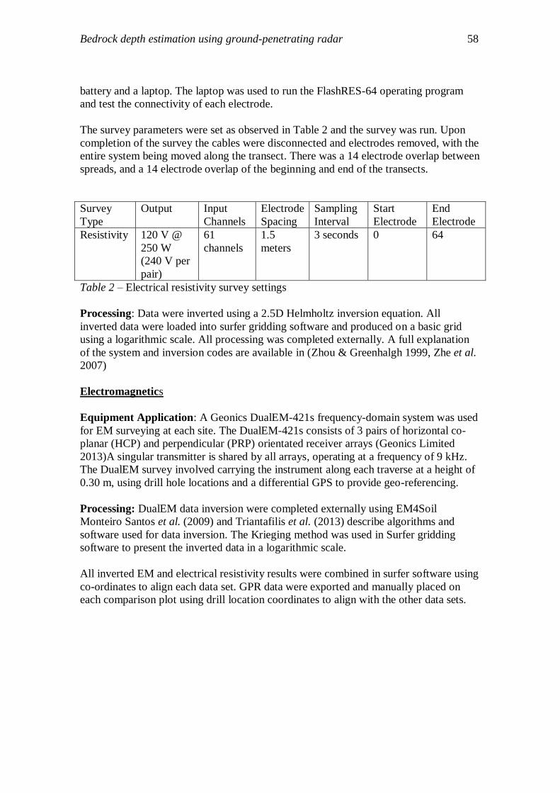
Bedrock depth estimation using ground-penetrating radar 58
battery and a laptop. The laptop was used to run the FlashRES-64 operating program
and test the connectivity of each electrode.
The survey parameters were set as observed in Table 2 and the survey was run. Upon
completion of the survey the cables were disconnected and electrodes removed, with the
entire system being moved along the transect. There was a 14 electrode overlap between
spreads, and a 14 electrode overlap of the beginning and end of the transects.
Survey
Type
Output Input
Channels
Electrode
Spacing
Sampling
Interval
Start
Electrode
End
Electrode
Resistivity 120 V @
250 W
(240 V per
pair)
61
channels
1.5
meters
3 seconds 0 64
Table 2 – Electrical resistivity survey settings
Processing: Data were inverted using a 2.5D Helmholtz inversion equation. All
inverted data were loaded into surfer gridding software and produced on a basic grid
using a logarithmic scale. All processing was completed externally. A full explanation
of the system and inversion codes are available in (Zhou & Greenhalgh 1999, Zhe et al.
2007)
Electromagnetics
Equipment Application: A Geonics DualEM-421s frequency-domain system was used
for EM surveying at each site. The DualEM-421s consists of 3 pairs of horizontal co-
planar (HCP) and perpendicular (PRP) orientated receiver arrays (Geonics Limited
2013)A singular transmitter is shared by all arrays, operating at a frequency of 9 kHz.
The DualEM survey involved carrying the instrument along each traverse at a height of
0.30 m, using drill hole locations and a differential GPS to provide geo-referencing.
Processing: DualEM data inversion were completed externally using EM4Soil
Monteiro Santos et al. (2009) and Triantafilis et al. (2013) describe algorithms and
software used for data inversion. The Krieging method was used in Surfer gridding
software to present the inverted data in a logarithmic scale.
All inverted EM and electrical resistivity results were combined in surfer software using
co-ordinates to align each data set. GPR data were exported and manually placed on
each comparison plot using drill location coordinates to align with the other data sets.

Bedrock depth estimation using ground-penetrating radar 59
Soil Analysis
The soil collected from each drill hole was analysed for the purpose of cross comparison
with the applied geophysical techniques. Often techniques will not perform as initially
anticipated in the field and soil analysis results will help to explain why certain
techniques show good quality data, while others may not. Anomalies and errors related
to equipment operation can also be mitigated by comparison with associated soil data.
4.4.1 Application: Each transect was marked with 20m intervals, which were used to
determine the drill sites. Push tube percussion drilling was used to drill to a maximum
depth of 9m, or to drill refusal. Removed samples were gathered and sub-sampled into
30cm depth intervals from 0cm to 150cm, and in 50cm depth intervals from 150cm to
drill refusal depth. Each sample bag was weighed in the field using a scale to obtain the
wet weight of the soil. The extent of weathering of each soil sample was described and
recorded.
The sample bags were labelled and placed into an oven for 2 weeks. Upon completion
of the drying process, the same scale was used to re-weigh the samples, giving an
absolute value for the moisture content of the soil. Each of the dry samples were
separated into two fractions using a 2 mm sieve. The >2 mm fractions were weighed
and set aside, as were the <2 mm fractions. 5 grams of the <2mm fraction was removed
and used for EC 1:5 salinity analysis. EC 1:5 analysis consisted of weighing exactly 5
grams of <2 mm soil to 25 grams distilled water, placing on a rotating drum at 25 rpm
for 1 hour. The samples were left to settle for 30 minutes before the EC 1:5 readings
were taken. A K=10 electrode was used for measurements in each sample and rinsed
with RO water between each reading. This method is further detailed in: Rayment, G.E., Higginson, F.R., 1992. Australian laboratory handbook of soil and water chemical methods. Australian Soil and Land Survey Handbook. Inkata Press, Melbourne.
All results were recorded and presented in excel spreadsheets.

Bedrock depth estimation using ground-penetrating radar 60
APPENDIX B:
SOIL ANALYSIS DATA

Bedrock depth estimation using ground-penetrating radar 61
Site 1: Rocky Paddock
Drill Hole Distance Along Coordinates
Total soil depth Moisture
E:C
1.5 Soil
Line (metres) Easting Northing Drill Depth increment wt. % μs/cm Horizon
1.01 0 311270 6156095 1.5 00/30 7.14 81.00
30/60 10.97 58.10
60/90 3.38 39.10
90/120 -0.42 30.20
120/150 -0.93 34.70
1.02 20 311258 6156079 1.5 00/30 1.95 113.70
30/60 8.93 65.70
60/90 2.33 43.20
90/120 8.54 61.30
120/150 3.96 76.60
1.03 40 311244 6156064 1.9 00/30 3.51 83.00
30/60 7.94 50.40
60/90 6.67 37.20
90/120 10.90 50.00
120/150 7.45 51.50
150/190 6.43 43.00
1.04 60 311230 6156051 1.35 00/30 -0.17 81.30 A
30/60 7.35 47.20 B
60/90 3.49 31.80 C
90/120 3.24 29.00 C
120/135 2.71 38.70 C
1.05 80 311215 6156038 1.5 00/30 3.86 199.80 A

Bedrock depth estimation using ground-penetrating radar 62
30/60 13.01 53.10 B
60/90 9.83 39.00 C
90/120 2.88 26.60 C
120/150 3.18 33.50 C
1.06 100 311201 6156024 1.8 00/30 1.51 100.60 A
30/60 11.99 58.00 B
60/90 14.01 48.10 B
90/120 10.04 40.40 C
120/150 5.54 33.50 C
150/180 4.77 28.70 C
1.07 120 311185 6156011 2 00/30 2.86 107.40 A
30/60 7.78 55.90 B
60/90 12.97 48.50 B
90/120 7.58 34.20 B
120/150 5.98 35.60 C
150/200 7.60 34.20 C
1.08 140 311170 6155999 2 00/30 1.48 70.20 A
30/60 4.41 45.30 A2
60/90 15.76 58.40 B
90/120 N/A 58.20 B
120/150 11.99 55.10 C
150/200 7.27 41.80 C
1.09 160 311155 6155987 4.7 00/30 1.83 135.60
30/60 13.16 60.50
60/90 12.35 57.10
90/120 12.49 60.40
120/150 2.96 38.60

Bedrock depth estimation using ground-penetrating radar 63
150/200 7.67 31.20
200/250 11.56 34.80
250/300 18.15 76.20
300/350 16.34 90.60
350/400 16.46 123.90
400/450 11.24 100.00
450/470 9.21 117.00
1.10 180 311139 6155973 1.2 00/30 3.12 138.40 A
30/60 4.28 51.90 A2
60/90 9.72 62.20 B/C
90/120 11.90 62.30 R
1.11 200 311124 6155961 3.3 00/30 1.31 108.90 A
30/60 13.29 63.10 B2
60/90 15.23 68.30 B2
90/120 11.34 61.30 B2
120/150 10.98 58.40 B2
150/200 10.61 60.40 C
200/250 10.91 55.40 C
250/300 11.46 44.90 C
300/330 6.67 76.00 C
1.12 220 311108 6155948 1.5 00/30 2.31 183.20 A
30/60 10.05 104.80 B
60/90 12.38 76.90 B
90/120 11.34 75.40 R
120/150 8.94 92.40 R
1.13 240 311093 6155937 3 00/30 2.20 104.80 A
30/60 13.64 104.00 B2

Bedrock depth estimation using ground-penetrating radar 64
60/90 8.54 59.30 B2
90/120 5.63 99.30 C
125/150 7.40 151.10 C
150/170 3.85 97.00 C
Site 2:
Chalkies Line 2.01 0 312622 6153444 1.9 00/30 11.83 121.50 A
30/60 13.64 78.30 B2
60/90 11.79 140.10 C
90/120 11.46 231.00 R
120/150 14.19 287.00 R
150/190 14.55 346.00 R
2.02 20 312641 6153440 1.7 00/30 7.06 150.00 A
30/60 12.49 69.30 B
60/90 9.12 69.90 C
90/120 8.63 102.90 R
120/150 6.89 171.90 R
150/170 4.51 143.80 R
2.03 33 312653 6153446 4.8 00/30 4.13 92.60 A
30/60 11.41 65.10 B2
60/90 7.51 55.10 B2
90/120 3.27 41.40 C
120/150 2.94 46.70 C
150/200 2.65 108.00 R
200/250 5.13 176.50 R
250/300 8.14 156.20 R

Bedrock depth estimation using ground-penetrating radar 65
300/350 10.53 84.10 R
350/400 11.07 94.10 R
400/450 8.39 79.70 R
450/480 7.57 68.50 R
2.04 40 312660 6153442 1.45 00/30 5.07 67.80 A
30/60 11.02 48.10 B
60/90 7.01 40.80 B
90/120 5.22 43.80 C
120/145 5.56 66.10 R
2.05 60 312680 6153437 2.4 00/30 2.94 93.00 A
30/60 9.99 121.00 B2
60/90 7.35 65.10 C
90/120 4.99 34.40 C
120/150 5.18 42.10 C
150/200 3.86 38.00 C
200/240 2.52 26.30 R
2.06 80 312699 6153439 7.3 00/30 5.57 57.30 A
30/60 7.51 38.30 A2
60/90 11.45 36.00 B2
90/120 2.80 25.40 C
120/150 2.67 33.80 C
150/200 6.32 79.00 C
200/250 7.10 44.60 C
250/300 8.09 48.20 C
300/350 7.21 45.70 C
350/400 5.96 43.00 C
400/450 6.68 47.90 C
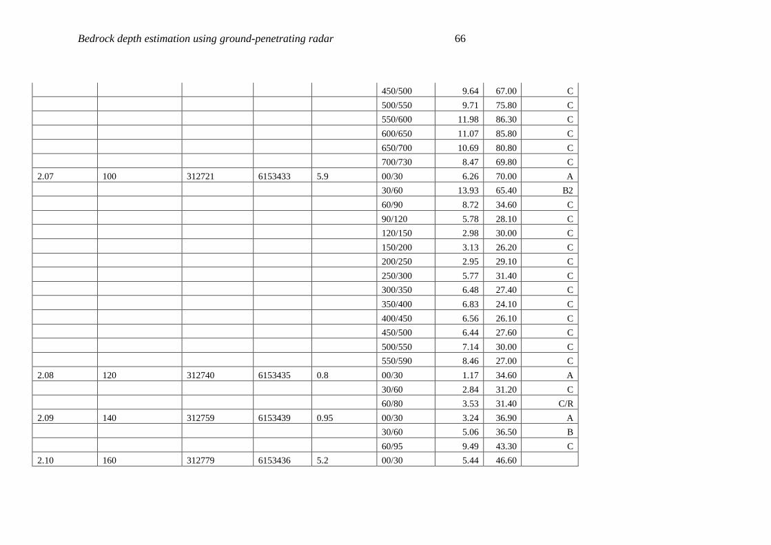
Bedrock depth estimation using ground-penetrating radar 66
450/500 9.64 67.00 C
500/550 9.71 75.80 C
550/600 11.98 86.30 C
600/650 11.07 85.80 C
650/700 10.69 80.80 C
700/730 8.47 69.80 C
2.07 100 312721 6153433 5.9 00/30 6.26 70.00 A
30/60 13.93 65.40 B2
60/90 8.72 34.60 C
90/120 5.78 28.10 C
120/150 2.98 30.00 C
150/200 3.13 26.20 C
200/250 2.95 29.10 C
250/300 5.77 31.40 C
300/350 6.48 27.40 C
350/400 6.83 24.10 C
400/450 6.56 26.10 C
450/500 6.44 27.60 C
500/550 7.14 30.00 C
550/590 8.46 27.00 C
2.08 120 312740 6153435 0.8 00/30 1.17 34.60 A
30/60 2.84 31.20 C
60/80 3.53 31.40 C/R
2.09 140 312759 6153439 0.95 00/30 3.24 36.90 A
30/60 5.06 36.50 B
60/95 9.49 43.30 C
2.10 160 312779 6153436 5.2 00/30 5.44 46.60

Bedrock depth estimation using ground-penetrating radar 67
30/60 13.31 45.30 A
60/90 10.82 30.90 B
90/120 11.33 32.30 B
120/150 10.78 36.20 B
150/200 7.02 32.20 C
200/250 10.94 31.10 C
250/300 13.17 44.30 C
300/350 12.80 34.10 C
350/400 11.75 29.90 C
400/450 13.64 30.90 C
450/500 12.88 33.00 C
500/520 11.90 40.80 R
2.11 180 312798 6153437 0.8 00/30 4.17 47.30 A
30/60 8.19 33.50 B
60/80 7.29 30.10 R
2.12 200 312817 6153439 1.4 00/30 3.58 72.80 A
30/60 12.34 46.30 B1
60/90 11.78 39.00 B2
90/120 10.88 45.60 C
120/140 10.23 56.10 R
2.13 220 312834 6153432 2.25 00/30 3.71 59.40 A
36/60 11.36 42.90 B2
60/90 12.40 34.60 B2
90/120 8.78 30.40 B2
120/150 8.57 35.40 C
150/200 12.23 64.20 C
200/225 10.94 53.20 R

Bedrock depth estimation using ground-penetrating radar 68
2.14 240 312859 6153431 2.3 00/30 2.50 46.30 A
30/60 7.42 32.10 B2
60/90 10.86 32.60 B2
90/120 4.92 34.20 B2
120/150 3.60 31.90 C
150/200 4.35 47.60 C
200/230 6.50 39.50 C
2.15 260 312879 6153430 1.35 00/30 4.93 57.90 A
30/60 9.89 38.30 B
60/90 10.63 47.20 B
90/120 7.68 47.60 C
120/135 7.84 73.40 C
2.16 280 312898 6153426 7.15 00/30 2.27 54.20 A
30/60 9.35 40.60 B2
60/90 8.65 36.10 B2
90/120 8.28 36.30 C
120/150 5.95 42.50 C
150/200 5.60 49.90 C
200/250 10.63 63.90 C
250/300 13.75 88.60 C
300/350 14.13 88.70 C
350/400 13.57 115.70 C
400/450 17.44 114.30 C
450/500 17.26 108.60 C
500/550 16.15 94.70 C
550/600 18.29 115.70 C
600/650 17.55 124.40 C

Bedrock depth estimation using ground-penetrating radar 69
650/700 19.28 121.10 C
700/715 19.25 125.50 C
2.17 300 312917 6153429 0.85 00/30 10.19 66.70 A/B
30/60 9.35 42.60 B2
60/85 9.51 58.50 B2/C
2.18 320 312938 6153428 1.05 00/30 10.15 97.10 A
30/60 15.15 62.20 B2
60/90 10.58 61.40 B2
90/105 9.68 72.00 C
2.19 340 312958 6153427 3.3 00/30 8.20 61.40 A/B
30/60 14.85 44.50 B
60/90 12.23 40.10 B
90/120 12.96 41.40 B
120/150 13.81 52.50 C
150/200 17.21 65.80 C
200/250 18.42 82.20 C
250/300 12.72 89.60 C
300/330 13.22 128.50 C
2.2 360 312978 6153426 1.5 00/30 4.58 45.20 A1
30/60 7.71 50.60 B1
60/90 13.53 43.40 B2
90/120 8.84 41.20 C
120/150 9.88 52.40 C/R
2.21 400 313019 6153422 1.5 00/30 5.09 52.80
30/60 16.41 60.20
60/90 17.28 63.10
90/120 16.80 76.60

Bedrock depth estimation using ground-penetrating radar 70
120/150 15.82 129.50
2.22 460 313079 6153420 6 00/30 3.54 70.80 A
30/60 7.90 61.60 B
60/90 9.99 61.80 B
90/120 9.73 56.70 C
120/150 9.59 79.80 C
150/200 13.76 251.00 C
200/250 8.49 231.70 C
250/300 9.42 449.00 C
300/350 9.46 N/A C
350/400 10.79 539.00 C
400/450 8.98 430.00 C
450/500 13.00 610.00 C/R
500/550 13.48 610.00 R
550/600 9.94 416.00 R
2.23 560 313179 6153416 0.6 00/30 11.86 67.80 A/B
30/60 12.89 113.40 B2
2.24 580 313200 6153418 1.25 00/30 5.92 N/A A
30/60 14.52 88.90 B2
60/90 13.69 108.10 B2
90/125 13.67 129.50 B2/R
Site 3:
Canham
Road
3.01 320 314285 6153745 0.65 00/30 1.40 31.50 A
30/65 3.03 36.60 C/R

Bedrock depth estimation using ground-penetrating radar 71
3.02 300 314268 6153749 0.5 00/30 2.37 44.80 A/B
30/50 2.05 40.90 B/R
3.03 280 314247 6153750 0.55 00/30 0.98 44.50 A/B
30/55 1.94 40.90 B/R
3.04 260 314228 6153748 0.4 00/40 1.05 62.50 A
3.05 240 314209 6153746 0.65 00/30 1.42 55.30 B
30/65 1.28 36.30 R
3.06 220 314190 6153746 2.9 00/30 1.55 37.60 A/B
30/60 2.84 30.80 B
60/90 12.06 36.40 B2
90/120 12.62 56.60 B2
120/150 14.86 71.20 B2
150/200 16.88 89.40 B2
200/250 17.15 100.60 B2
250/290 15.00 110.60 B2/R
3.07 200 314169 6153746 1.6 00/30 0.95 33.10
30/60 19.01 73.50
60/90 17.06 65.50
90/120 16.12 67.80
120-160 17.09 93.60
3.08 180 314149 6153746 3.1 00/30 9.03 54.00 A/B
30/60 15.54 45.20 B
60/90 9.13 44.90 B
90/120 15.48 50.10 B
120/150 15.08 51.30 B
150/200 14.48 55.30 B
200/250 13.54 63.90 B

Bedrock depth estimation using ground-penetrating radar 72
250/310 10.97 65.60 B/R
3.09 160 314131 6153744 2.9 00/30 15.79 66.00 B2
30/60 16.02 37.30 B2
60/90 10.90 37.50 B2
90/120 15.96 44.30 B2
120/150 14.64 50.50 B2
150/200 16.01 63.00 B2
200/250 15.93 74.40 B2
250/290 12.55 204.80 B2/R
3.1 140 314114 6153745 1.7 00/30 5.54 59.70 B2
30/60 14.82 N/A B2
60/90 14.10 45.00 B2
90/120 11.40 47.70 C
120/150 7.10 58.00 C
150/170 5.11 64.20 R
3.11 120 314092 6153741 4.2 00/30 2.79 50.70 A1
30/60 11.02 51.90 B1
60/90 10.60 43.20 B2
90/120 8.05 37.20 B2
120/150 4.81 38.20 C
150/200 7.51 44.80 C
200/250 5.02 45.20 C
250/300 8.12 65.10 C
300/350 5.01 31.60 C
350/400 4.09 29.10 C
400/420 4.29 40.50 C
3.12 100 314073 6153741 1.5 00/30 4.65 60.70 A/B
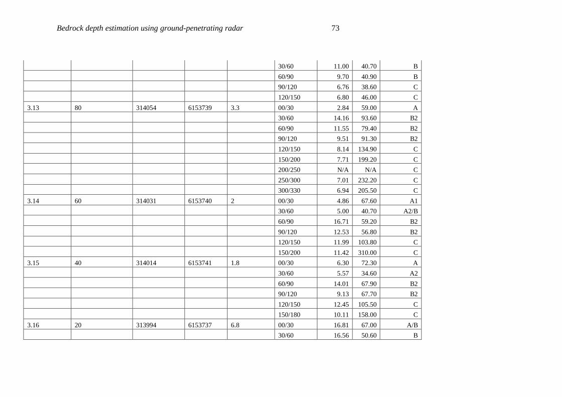
Bedrock depth estimation using ground-penetrating radar 73
30/60 11.00 40.70 B
60/90 9.70 40.90 B
90/120 6.76 38.60 C
120/150 6.80 46.00 C
3.13 80 314054 6153739 3.3 00/30 2.84 59.00 A
30/60 14.16 93.60 B2
60/90 11.55 79.40 B2
90/120 9.51 91.30 B2
120/150 8.14 134.90 C
150/200 7.71 199.20 C
200/250 N/A N/A C
250/300 7.01 232.20 C
300/330 6.94 205.50 C
3.14 60 314031 6153740 2 00/30 4.86 67.60 A1
30/60 5.00 40.70 A2/B
60/90 16.71 59.20 B2
90/120 12.53 56.80 B2
120/150 11.99 103.80 C
150/200 11.42 310.00 C
3.15 40 314014 6153741 1.8 00/30 6.30 72.30 A
30/60 5.57 34.60 A2
60/90 14.01 67.90 B2
90/120 9.13 67.70 B2
120/150 12.45 105.50 C
150/180 10.11 158.00 C
3.16 20 313994 6153737 6.8 00/30 16.81 67.00 A/B
30/60 16.56 50.60 B

Bedrock depth estimation using ground-penetrating radar 74
60/90 12.36 37.20 B/C
90/120 9.99 34.70 C
120/150 8.43 35.30 C
150/200 7.93 37.10 C
200/250 6.90 39.60 C
250/300 9.21 78.50 C
300/350 8.78 141.40 C
350/400 10.01 307.00 C
400/450 10.78 404.00 C
450/500 14.59 366.00 C
500/550 15.14 387.00 C
550/600 17.13 519.00 C
600/650 20.01 682.00 C
650/680 17.63 602.00 C
3.17 0 313973 6153736 3.1 00/30 9.71 55.00 B
30/60 6.96 38.90 C
60/90 5.22 36.50 C
90/120 6.27 35.00 C
120/150 5.91 37.20 C
150/200 4.72 36.40 C
200/250 6.32 39.60 C
250/300 7.99 53.70 C
300/310 8.21 61.00 R

Bedrock depth estimation using ground-penetrating radar 75
APPENDIX C:
GPR RADARGRAMS FOR SITE 1
All GPR data can be made available electronically upon request to the author.

Bedrock depth estimation using ground-penetrating radar 76
Raw data is presented in greyscale. Processed data is presented in colour.

Bedrock depth estimation using ground-penetrating radar 77

Bedrock depth estimation using ground-penetrating radar 78

Bedrock depth estimation using ground-penetrating radar 79

Bedrock depth estimation using ground-penetrating radar 80
APPENDIX D:
GPR RADARGRAMS FOR SITE 2
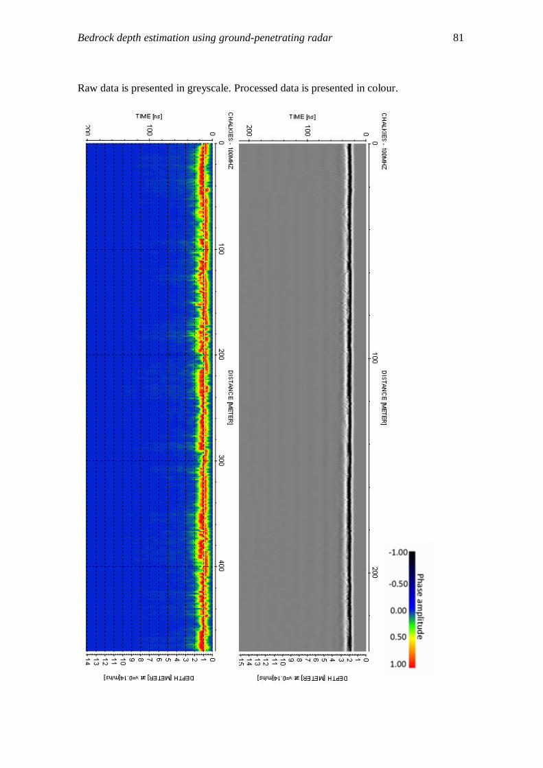
Bedrock depth estimation using ground-penetrating radar 81
Raw data is presented in greyscale. Processed data is presented in colour.
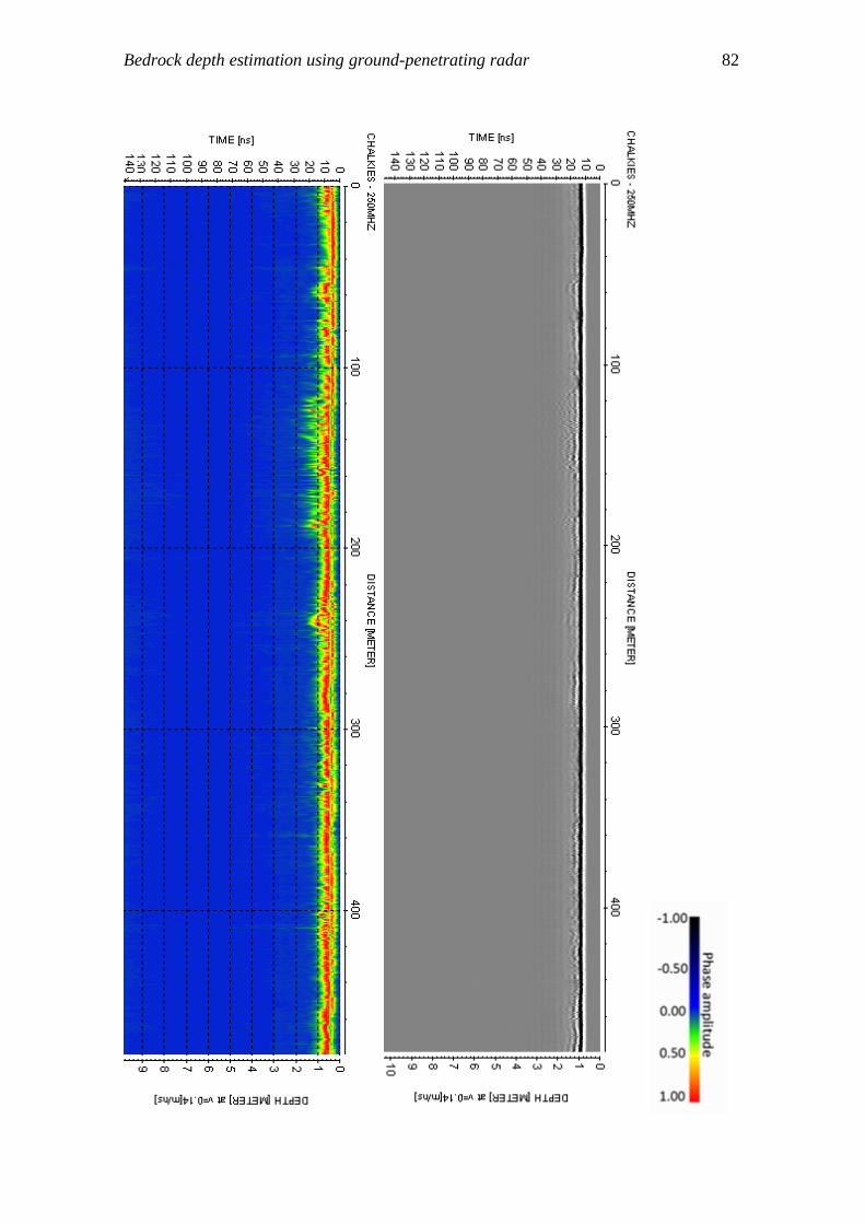
Bedrock depth estimation using ground-penetrating radar 82

Bedrock depth estimation using ground-penetrating radar 83

Bedrock depth estimation using ground-penetrating radar 84

Bedrock depth estimation using ground-penetrating radar 85
APPENDIX E:
GPR RADARGRAMS FOR SITE 3

Bedrock depth estimation using ground-penetrating radar 86
Raw data is presented in greyscale. Processed data is presented in colour.

Bedrock depth estimation using ground-penetrating radar 87
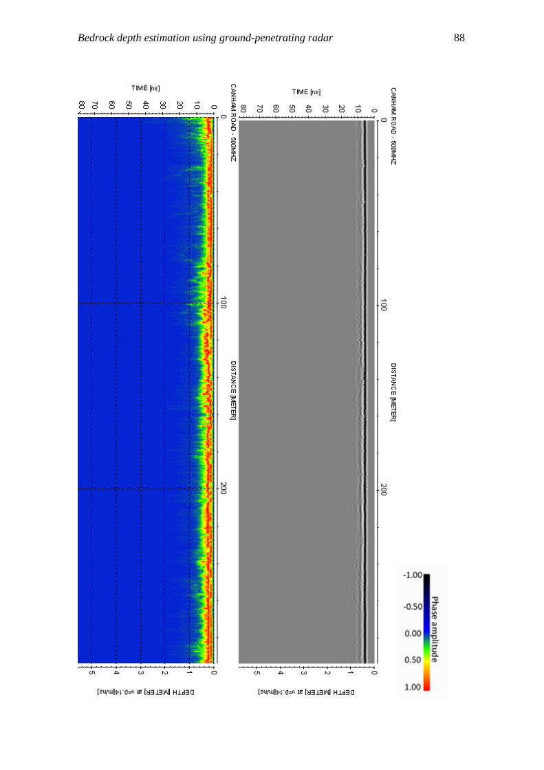
Bedrock depth estimation using ground-penetrating radar 88

Bedrock depth estimation using ground-penetrating radar 89