estimating abundance in populations
TRANSCRIPT
PART ONE
ESTIMATING ABUNDANCE IN
ANIMAL AND PLANT
POPULATIONS
How many are there? This question is the central question of many ecological
studies. If you wish to harvest a lake trout population, one helpful bit of
information is the size of the population you wish to harvest. If you are trying to
decide whether to spray a pesticide for aphids on a crop, you may wish to
know how many aphids are living on your crop plants. If you wish to measure
the impact of lion predation on a zebra population, you will need to know the
size of both the lion and the zebra populations.
The cornerstone of many ecological studies is an estimate of the
abundance of a particular population. This is true for both population ecology,
in which interest centers on individual species, and community ecology, in
which interest centers on groups of species and, thus, the estimation problem
is more complex. Note that some ecological studies do not require an estimate
of abundance, so before you begin with the labor of estimating the size of a
population, you should have a clear idea why you need these data. Estimates
of abundance themselves are not valuable, and a large book filled with
estimates of the abundance of every species on earth as of January 1, 1997
would be a good conversation piece but not science.
Abundance can be measured in two ways. Absolute density is the
number of organisms per unit area or volume. A red deer density of four deer
per square kilometer is an absolute density. Relative density is the density of
one population relative to that of another population. Blue grouse may be
more common in a block of recently burned woodland than in a block of
mature woodland. Relative density estimates are usually obtained with some
biological index that is correlated with absolute density. Relative density may
be adequate for many ecological problems, and should always be used when
adequate because it is much easier and cheaper to determine than absolute
density.
Absolute density must be obtained for any detailed population study in
which one attempts to relate population density to reproductive rate, or any
other vital statistic. The analysis of harvesting strategies may demand
information on absolute numbers. All community studies which estimate
energy flow or nutrient cycles require reliable estimates of absolute density.

Part 1 Page 21
The sequence of decisions by which one decides how to estimate
absolute density is outlined in Figure A. Many factors - ecological, economic,
and statistical - enter into a decision about how to proceed in estimating
population size. Figure A thus gives relative guidance rather than absolute
rules. Quadrat counts and spatial distribution methods are usually chosen in
plant studies. Many vertebrate studies use mark-recapture techniques. Fish
and wildlife populations that are exploited can be estimated by a special set of
techniques applicable to harvested populations. There is a rapidly
accumulating store of ecological wisdom for estimating populations of different
animal and plant species, and if you are assigned to study elephant
populations, you should begin by finding out how other elephant ecologists
have estimated population size in this species. But do not stop there. Read the
next five chapters and you may find the conventional wisdom needs updating.
Fresh approaches and new improvements in population estimation occur often
enough that ecologists cannot yet become complacent about knowing the best
way to estimate population size in each species.
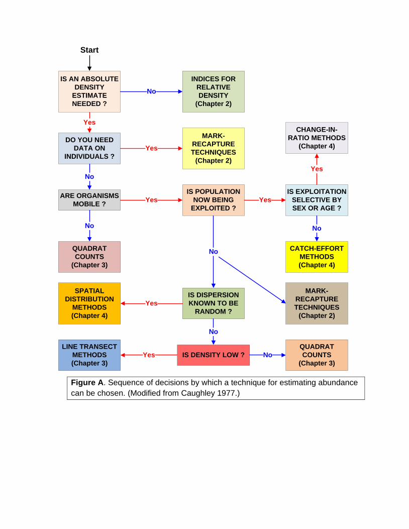
Figure A. Sequence of decisions by which a technique for estimating abundance
can be chosen. (Modified from Caughley 1977.)
IS AN ABSOLUTE
DENSITY
ESTIMATE
NEEDED ?
DO YOU NEED
DATA ON
INDIVIDUALS ?
ARE ORGANISMS
MOBILE ?
QUADRAT
COUNTS
(Chapter 3)
SPATIAL
DISTRIBUTION
METHODS
(Chapter 4)
LINE TRANSECT
METHODS
(Chapter 3)
MARK-
RECAPTURE
TECHNIQUES
(Chapter 2)
INDICES FOR
RELATIVE
DENSITY
(Chapter 2)
CHANGE-IN-
RATIO METHODS
(Chapter 4)
IS POPULATION
NOW BEING
EXPLOITED ?
IS EXPLOITATION
SELECTIVE BY
SEX OR AGE ?
CATCH-EFFORT
METHODS
(Chapter 4)
IS DISPERSION
KNOWN TO BE
RANDOM ?
IS DENSITY LOW ?
QUADRAT
COUNTS
(Chapter 3)
Start
Yes
No
Yes
No
Yes
No
No
Yes
No
Yes No
Yes
No
Yes
MARK-
RECAPTURE
TECHNIQUES
(Chapter 2)
Chapter 2
ESTIMATING ABUNDANCE AND DENSITY:
MARK-RECAPTURE TECHNIQUES
(Version 6, 21 December 2016) Page
2.1 PETERSEN METHOD ........................................................................................ 24
2.1.1 Confidence Intervals for the Petersen Method ......................................... 26
2.1.2 Sample Size Needed for Petersen Estimates ........................................... 34
2.1.3 Assumptions of Petersen Method ............................................................. 39
2.2 SCHNABEL METHOD ....................................................................................... 42
2.2.1 Confidence Intervals for Schnabel Estimates .......................................... 44
2.2.2 Assumptions of the Schnabel Method ....................................................... 49
2.3 PROGRAM CAPTURE AND PROGRAM MARK .............................................. 52
2.4 CORMACK-JOLLY-SEBER METHOD .............................................................. 60
2.4.1 Confidence Intervals for Cormack-Jolly-Seber Estimates ....................... 66
2.4.2 Assumptions of the Cormack-Jolly-Seber Method .................................. 70
2.5 PLANNING A MARK-RECAPTURE STUDY ..................................................... 71
2.6 WHAT TO DO IF NOTHING WORKS ................................................................ 74
2.7 SUMMARY ......................................................................................................... 77
SELECTED READING .............................................................................................. 78
QUESTIONS AND PROBLEMS ............................................................................... 78
One way to estimate the size of a population is to capture and mark individuals from the
population, and then to resample to see what fraction of individuals carry marks.
John Graunt first used this simple principle to estimate the human population of
London in 1662. The first ecological use of mark-and-recapture was carried out by
the Danish fisheries biologist C.G.J. Petersen in 1896 (Ricker 1975). Tagging of fish
was first used to study movements and migration of individuals, but Petersen
realized that tagging could also be used to estimate population size and to measure
mortality rates. Fisheries biologists were well advanced over others in applying
these methods. Lincoln (1930) used mark-recapture to estimate the abundance of
ducks from band returns, and Jackson (1933) was the first entomologist to apply
Chapter 2 Page 24
mark-recapture methods to insect populations. This chapter concentrates on the
mark-and-recapture techniques which are used most often when data are required
on individual organisms that are highly mobile. The strength of mark-and-recapture
techniques is that they can be used to provide information on birth, death, and
movement rates in addition to information on absolute abundance. The weakness of
these techniques is that they require considerable time and effort to get the required
data and, to be accurate, they require a set of very restrictive assumptions about the
properties of the population being studied. Seber (1982), Otis et al. (1978), Pollock
et al. (1990) and Amstrup et al. (2006) have described mark-and-recapture methods
in great detail, and this chapter is an abstract of the more common methods they
describe.
Mark-and-recapture techniques may be used for open or closed populations. A
closed population is one which does not change in size during the study period, that
is, one in which the effects of births, deaths, and movements are negligible. Thus
populations are typically closed over only a short period of time. An open population
is the more usual case, a population changing in size and composition from births,
deaths, and movements. Different methods must be applied to open and closed
populations, and I will discuss five cases in this chapter:
Closed populations
1. Single marking, single recapture - Petersen method
2. Multiple markings and recaptures - Schnabel method
3. Program CAPTURE and Program MARK
Open populations
1. Multiple census – Cormack-Jolly-Seber method.
Robust methods
1. Combining information from closed and open methods.
2.1 PETERSEN METHOD
The Petersen method is the simplest mark-and-recapture method because it is
based on a single episode of marking animals, and a second single episode of
recapturing individuals. The basic procedure is to mark a number of individuals over
a short time, release them, and then to recapture individuals to check for marks. All
individuals can be marked in the same way. The second sample must be a random
sample for this method to be valid; that is, all individuals must have an equal chance
of being captured in the second sample, regardless of whether they are marked or
not. The data obtained are
M = Number of individuals marked in the first sample
C = Total number of individuals captured in the second sample
R = Number of individuals in second sample that are marked.
From these three variables, we need to obtain an estimate of
Chapter 2 Page 25
N = Size of population at time of marking
By a proportionality argument, we obtain:
N C
M R=
or transposing:
ˆ C MN
R= (2.1)
where N̂ = Estimate of population size at time of marking*
and the other terms are defined above.
This formula is the "Petersen estimate" of population size and has been widely
used because it is intuitively clear. Unfortunately, formula (2.1) produces a biased
estimator of population size, tending to overestimate the actual population. This bias
can be large for small samples, and several formulae have been suggested to
reduce this bias. Seber (1982) recommends the estimator:
( )( )( )
+1 1ˆ = - 11
M CN
R
+
+ (2.2)
which is unbiased if (M + C) > N and nearly unbiased if there are at least seven
recaptures of marked animals (R > 7). This formula assumes sampling without
replacement (see page 000) in the second sample, so any individual can only be
counted once.
In some ecological situations, the second sample of a Petersen series is taken
with replacement so that a given individual can be counted more than once. For
example, animals may be merely observed at the second sampling and not
captured. For these cases the size of the second sample (C) can be even larger
than total population size (N) because individuals might be sighted several times. In
this situation we must assume that the chances of sighting a marked animal are on
the average equal to the chances of sighting an unmarked animal. The appropriate
estimator from Bailey (1952) is:
( )( )
+1ˆ = +1
M CN
R (2.3)
which differs only very slightly from equation (2.2) and is nearly unbiased when the
number of recaptures (R) is 7 or more.
* A ^ over a variable means "an estimate of".

Chapter 2 Page 26
2.1.1 Confidence Intervals for the Petersen Method
How reliable are these estimates of population size? To answer this critical
question, a statistician constructs confidence intervals around the estimates. A
confidence interval is a range of values which is expected to include the true
population size a given percentage of the time. Typically the given percentage is
95% but you can construct 90% or 99% confidence intervals, or any range you wish.
The high and low values of a confidence interval are called the confidence limits.
Clearly, one wants confidence intervals to be as small as possible, and the
statistician's job is to recommend confidence intervals of minimal size consistent
with the assumptions of the data at hand.
Confidence intervals are akin to gambling. You can state that the chances of
flipping a coin and getting "heads" is 50%, but after the coin is flipped, it is either
"heads" or "tails". Similarly, after you have estimated population size by the
Petersen method and calculated the confidence interval, the true population size
(unfortunately not known to you!) will either be inside your confidence interval or
outside it. You cannot know which, and all the statistician can do is tell you that on
the average 95% of confidence intervals will cover the true population size. Alas,
you only have one estimate, and on the average does not tell you whether your one
confidence interval is lucky or unlucky.
Confidence intervals are an important guide to the precision of your estimates.
If a Petersen population estimate has a very wide confidence interval, you should
not place too much faith in it. If you wish you can take a larger sample next time and
narrow the confidence limits. But remember that even when the confidence interval
is narrow, the true population size may sometimes be outside the interval. Figure 2.1
illustrates the variability of Petersen population estimates from artificial populations
of known size, and shows that some random samples by chance produce
confidence intervals that do not include the true value.
Several techniques of obtaining confidence intervals for Petersen estimates of
population size are available, and the particular one to use for any specific set of
data depends upon the size of the population in relation to the samples we have
taken. Seber (1982) gives the following general guide:

Chapter 2 Page 27
Is the ratio of
R/C > 0.10 ?
Is the number of
recaptures
R > 50 ?
Use binomial
confidence
intervals
no
Use Poisson
confidence
intervals
yes
yes
no
Use the normal
approximation
Petersen estimatesC = 50
Population estimate
600 800 1000 1200 1400 1600
Fre
qu
en
cy
0
10
20
30
40
50
60
70
80
Petersen estimatesC = 400
Population estimate
600 800 1000 1200 1400 1600
Fre
qu
en
cy
0
20
40
60
80
100
Chapter 2 Page 28
Figure 2.1 Petersen population estimates for an artificial population of N = 1000.
Five hundred replicate samples were drawn. In both cases M = 400 individuals
were marked in the first sample. (a) Samples of C = 50 were taken repeatedly for
the second sample. A total of 13 estimates out of 500 did not include the known
population size of 1000 (estimates below 705 or above 1570). (b) Samples of C =
400 were taken for the second sample. A total of 22 estimates out of 500 did not
include the known population size (estimates below 910 or above 1105). Note the
wide range of estimates of population size when the number of animals recaptured
is small.
Poisson Confidence Intervals We discuss the Poisson distribution in detail in Chapter
4 (page 000), and we are concerned here only with the mechanics of determining
confidence intervals for a Poisson variable.
Table 2.1 provides a convenient listing of values for obtaining 95% confidence
intervals based on the Poisson distribution. An example will illustrate this technique.
If I mark 600 (M) and then recatch a total of 200 (C) animals, 13 (R) of which are
marked, from Table 2.1:
lower 95% confidence limit of R when R is 13 = 6.686
upper 95% limit of R when R is 13 = 21.364
and the 95% confidence interval for estimated population size (sampling without
replacement) is obtained by using these values of R in equation (2.2):
( )( )601 201ˆLower 95% confidence limit on = - 1 = 540221.364 1
N+
( )( )601 201ˆUpper 95% confidence limit on = - 1 = 15,7166.686 1
N+
Table 2.1 Confidence limits for a Poisson frequency distribution. Given the number of
organisms observed (x), this table provides the upper and lower limits from the
Poisson distribution. This table cannot be used unless you are sure the observed
counts are adequately described by a Poisson distribution.
95% 99% 95% 99%
x Lower Upper Lower Upper x Lower Upper Lower Upper
0 0 3.285 0 4.771 51 37.67 66.76 34.18 71.56
1 0.051 5.323 0.010 6.914 52 38.16 66.76 35.20 73.20
2 0.355 6.686 0.149 8.727 53 39.76 68.10 36.54 73.62
3 0.818 8.102 0.436 10.473 54 40.94 69.62 36.54 75.16
4 1.366 9.598 0.823 12.347 55 40.94 71.09 37.82 76.61
Chapter 2 Page 29
5 1.970 11.177 1.279 13.793 56 41.75 71.28 38.94 77.15
6 2.613 12.817 1.785 15.277 57 43.45 72.66 38.94 78.71
7 3.285 13.765 2.330 16.801 58 44.26 74.22 40.37 80.06
8 3.285 14.921 2.906 18.362 59 44.26 75.49 41.39 80.65
9 4.460 16.768 3.507 19.462 60 45.28 75.78 41.39 82.21
10 5.323 17.633 4.130 20.676 61 47.02 77.16 42.85 83.56
11 5.323 19.050 4.771 22.042 62 47.69 78.73 43.91 84.12
12 6.686 20.335 4.771 23.765 63 47.69 79.98 43.91 85.65
13 6.686 21.364 5.829 24.925 64 48.74 80.25 45.26 87.12
14 8.102 22.945 6.668 25.992 65 50.42 81.61 46.50 87.55
15 8.102 23.762 6.914 27.718 66 51.29 83.14 46.50 89.05
16 9.598 25.400 7.756 28.852 67 51.29 84.57 47.62 90.72
17 9.598 26.306 8.727 29.900 68 52.15 84.67 49.13 90.96
18 11.177 27.735 8.727 31.839 69 53.72 86.01 49.13 92.42
19 11.177 28.966 10.009 32.547 70 54.99 87.48 49.96 94.34
20 12.817 30.017 10.473 34.183 71 54.99 89.23 51.78 94.35
21 12.817 31.675 11.242 35.204 72 55.51 89.23 51.78 95.76
22 13.765 32.277 12.347 36.544 73 56.99 90.37 52.28 97.42
23 14.921 34.048 12.347 37.819 74 58.72 91.78 54.03 98.36
24 14.921 34.665 13.793 38.939 75 58.72 93.48 54.74 99.09
25 16.768 36.030 13.793 40.373 76 58.84 94.23 54.74 100.61
26 16.77 37.67 15.28 41.39 77 60.24 94.70 56.14 102.16
27 17.63 38.16 15.28 42.85 78 61.90 96.06 57.61 102.42
28 19.05 39.76 16.80 43.91 79 62.81 97.54 57.61 103.84
29 19.05 40.94 16.80 45.26 80 62.81 99.17 58.35 105.66
30 20.33 41.75 18.36 46.50 81 63.49 99.17 60.39 106.12
31 21.36 43.45 18.36 47.62 82 64.95 100.32 60.39 107.10
32 21.36 44.26 19.46 49.13 83 66.76 101.71 60.59 108.61
33 22.94 45.28 20.28 49.96 84 66.76 103.31 62.13 110.16
34 23.76 47.02 20.68 51.78 85 66.76 104.40 63.63 110.37
35 23.76 47.69 22.04 52.28 86 68.10 104.58 63.63 111.78
36 25.40 48.74 22.04 54.03 87 69.62 105.90 64.26 113.45
37 26.31 50.42 23.76 54.74 88 71.09 107.32 65.96 114.33
38 26.31 51.29 23.76 56.14 89 71.09 109.11 66.81 114.99
39 27.73 52.15 24.92 57.61 90 71.28 109.61 66.81 116.44
Chapter 2 Page 30
40 28.97 53.72 25.83 58.35 91 72.66 110.11 67.92 118.33
41 28.97 54.99 25.99 60.39 92 74.22 111.44 69.83 118.33
42 30.02 55.51 27.72 60.59 93 75.49 112.87 69.83 119.59
43 31.67 56.99 27.72 62.13 94 75.49 114.84 70.05 121.09
44 31.67 58.72 28.85 63.63 95 75.78 114.84 71.56 122.69
45 32.28 58.84 29.90 64.26 96 77.16 115.60 73.20 122.78
46 34.05 60.24 29.90 65.96 97 78.73 116.93 73.20 124.16
47 34.66 61.90 31.84 66.81 98 79.98 118.35 73.62 125.70
48 34.66 62.81 31.84 67.92 99 79.98 120.36 75.16 127.07
49 36.03 63.49 32.55 69.83 100 80.25 120.36 76.61 127.31
50 37.67 64.95 34.18 70.05
Source: Crow and Gardner, 1959.
When x > 100 use the normal approximation:
95% confidence limits of x:
Lower limit = 𝑥 − 0.94 − 1.96√𝑥 − 0.02
Upper limit = 𝑥 + 1.94 + 1.96√𝑥 − 0.98
99% confidence limits of x:
Lower limit = 𝑥 − 1.99 − 2.576√𝑥 − 0.33
Upper limit = 𝑥 + 2.99 + 2.576√𝑥 − 1.33
Normal Approximation Confidence Intervals This method is essentially a "large
sample" method which obtains a confidence interval on the fraction of marked
animals in the second catch (R/C). It should be used only when R is above 50. The
confidence interval for (R/C) is defined by the formula:
( )( )( )( )
1 1 1 +
1 2
R RfR C Cz
C C C
− −
−
(2.4)
where f = fraction of total population sampled in the second sample = RM
12C
= correction for continuity
z = standard normal deviate for (1- ) level of confidence
= 1.96 (for 95% confidence limits)
= 2.576 (for 99% confidence limits)
Chapter 2 Page 31
For large samples and a large population size, both the finite population correction (1-f)
and the correction for continuity are negligible, and this formula for the normal
approximation to the binomial simplifies to:
( )( )( )
1
1
R RR C C
zC C
−
− (2.5)
The constant z defines 100 (1- ) percent confidence limits, and values can be
substituted from tables of the standard normal distribution (z) (e.g. Zar 1996, pg.
19). For example, for 80% confidence limits replace z with the constant 1.2816.
One example will illustrate this method. If I mark 1800 animals (M) and catch at
the second sampling a total of 800 (C), of which 73 (R) are already tagged, from
formula (2.4) for 95% confidence limits:
( )( ) ( )
( ) ( )
73 73 731 173 11800 800 8001.96 +
800 800 1 2 800
− −
−
= 0.09125 ± 0.020176
and the 95% confidence interval for (R/C) is 0.07107 to 0.111426. To obtain a 95%
confidence interval for the estimated population size we use these limits for R/C in
equation (2.1):
ˆ C M
NR
=
Lower 95% confidence limit on ( )1ˆ= 1800 =16,154
0.111426N
Upper 95% confidence limit on ( )1ˆ= 1800 =25,326
0.07107N
Binomial Confidence Intervals Binomial confidence intervals for the fraction of
marked animals (R/C) can be obtained most easily graphically from Figure 2.2. The
resulting confidence interval will be approximate but should be adequate for most
ecological data. For example, suppose I mark 50 birds (M), and then capture 22 (C)
birds of which 14 (R) are marked. The fraction of marked animals (R/C) is 14/22 or
0.64. Move along the X-axis (Sample Proportion) to 0.64, and then move up until
you intercept the first sample size line of C, or 22. Then read across to the Y-axis
(Population Proportion) to obtain 0.40, the lower 95% confidence limit for (R/C). Now
repeat the procedure to intercept the second sample size line of C, or 22. Reading
across again, you find on the Y-axis 0.83, the upper 95% confidence limit for (R/C).
Chapter 2 Page 32
These confidence limits can be converted to confidence limits for population
size (N) by the use of these limits for (R/C) in formula (2.1), exactly as described
above (page 31). We use these limits for R/C in equation (2.1):
ˆ C M
NR
=
Lower 95% confidence limit on ( )1ˆ 50 60
0.83N = =
Upper 95% confidence limit on ( )1ˆ 50 125
0.40N = =
Binomial 95% Confidence Limits
Sample proportion p
0.0 0.1 0.2 0.3 0.4 0.5 0.6 0.7 0.8 0.9 1.0
Po
pu
lati
on
pro
po
rtio
n
0.0
0.1
0.2
0.3
0.4
0.5
0.6
0.7
0.8
0.9
1.0
Figure 2.2 Upper and lower 95% confidence limits for the populationproportion.
5
10
15
2030
50
100
200
500
200
100
50
30
20
15
10
5
Chapter 2 Page 33
Figure 2.2 Upper and lower 95% confidence limits for a population proportion.
Confidence limits are read off the y-axis for an observed value of p on the x-axis.
Sample sizes are marked on the contour lines.
Alternatively and more exactly, binomial confidence limits can be calculated
using Program EXTRAS (Appendix 2, page 000) which uses the Wilson method
formulae given in Brown et al. (2001). For the bird example above, the Wilson
method provides the exact 95% confidence limits of 0.430 to 0.803, compared with
the slightly less accurate 0.40 to 0.83 read off Figure 2.2 visually. Brown et al.
(2001) discuss all the problems of the different methods of calculating binomial
confidence limits, and conclude that the Wilson method is the best both for small
and large sample sizes.
Program RECAP (Appendix 2, page 000) computes the Petersen estimate of
population size and the appropriate confidence interval according to the
recommendations of Seber (1982). Box 2.1 illustrates how the Petersen
calculations are done.
Box 2.1 PETERSEN METHOD OF POPULATION ESTIMATION
Green and Evans (1940) estimated the size of a snowshoe hare population at Lake Alexander, Minnesota, in the winter of 1932-33 from these live-trapping data (sampling without replacement):
M = 948 hares caught and tagged in first sample C = 421 total caught in second sample R = 167 marked hares in second sample
Biased Estimator (equation 2.1)
ˆ C MN
R=
( )( )421 9482390 hares
167= =
Unbiased Estimator (equation 2.2)
( )( )( )
+1 1ˆ - 11
M CN
R
+=
+
( )( )421 1 948 1 = - 1 = 2383 hares
167 1
+ +
+
Confidence Interval
Chapter 2 Page 34
R/C = 0.3967 so we use a binomial confidence interval. We can read the approximate confidence limits off Figure 2.2, and this provides visual estimates of 0.35 to 0.45 as 95% confidence limits.
We thus obtain a confidence interval for population size as:
Lower 95% confidence limit on ( )
1ˆ 948 21070.45
CN M
R= = =
Upper 95% confidence limit on ( )
1ˆ 948 27090.35
CN M
R= = =
If we use the more exact equations for binomial confidence limits given by the Wilson method (Brown et al. 2001) we obtain 95% confidence limits of 0.351 to 0.444 for the ratio of R/C, and narrower confidence limits of 2135 to 2700 individuals.
These calculations can be done in Program RECAP (Appendix 2, page 000)
2.1.2 Sample Size Needed for Petersen Estimates
Let us now turn the Petersen method upside down and ask, given a rough
estimate of population size (N), how large a sample do I need to take to get a good
estimate of abundance. This is a key question for a great deal of ecological work
that uses mark-recapture techniques, and should be asked before a study is done,
not afterward. Two preliminary bits of information must be given before an answer to
the sample size question can be given precisely:
1. Initial estimate of population size (N)
2. Accuracy desired in Petersen estimate
The first requirement is the usual statistical one of "knowing the answer before
you do any of the work", but this can be a very rough, order-of-magnitude guess.
The only rule is to guess on the high side if you wish to be conservative.
The second requirement needs a quantitative definition of accuracy. We desire
our estimate of population size to be within a certain range of the true value, and we
call this the accuracy (A):
Estimated population size - true population size
100True population size
A
=
where A = accuracy of an estimate (as a percentage)
Thus we may wish our estimate to be within ± 10% accuracy. We cannot
guarantee this accuracy all the time, and we must allow a probability (α) of not
Chapter 2 Page 35
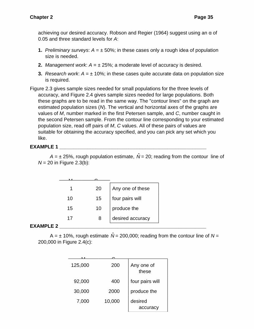
achieving our desired accuracy. Robson and Regier (1964) suggest using an α of
0.05 and three standard levels for A:
1. Preliminary surveys: A = ± 50%; in these cases only a rough idea of population
size is needed.
2. Management work: A = ± 25%; a moderate level of accuracy is desired.
3. Research work: A = ± 10%; in these cases quite accurate data on population size
is required.
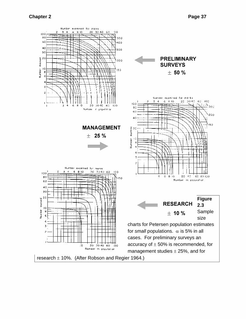
Figure 2.3 gives sample sizes needed for small populations for the three levels of
accuracy, and Figure 2.4 gives sample sizes needed for large populations. Both
these graphs are to be read in the same way. The "contour lines" on the graph are
estimated population sizes (N). The vertical and horizontal axes of the graphs are
values of M, number marked in the first Petersen sample, and C, number caught in
the second Petersen sample. From the contour line corresponding to your estimated
population size, read off pairs of M, C values. All of these pairs of values are
suitable for obtaining the accuracy specified, and you can pick any set which you
like.
EXAMPLE 1 _____________________________________________________
A = ± 25%, rough population estimate, N̂ = 20; reading from the contour line of
N = 20 in Figure 2.3(b):
EXAMPLE 2 _____________________________________________________
A = ± 10%, rough estimate N̂ = 200,000; reading from the contour line of N =
200,000 in Figure 2.4(c):
M C
1 20 Any one of these
10 15 four pairs will
15 10 produce the
17 8 desired accuracy
M C
125,000 200 Any one of
these
92,000 400 four pairs will
30,000 2000 produce the
7,000 10,000 desired
accuracy

Chapter 2 Page 36
Chapter 2 Page 37
Figure
2.3
Sample
size
charts for Petersen population estimates
for small populations. is 5% in all
cases. For preliminary surveys an
accuracy of 50% is recommended, for
management studies 25%, and for
research 10%. (After Robson and Regier 1964.)
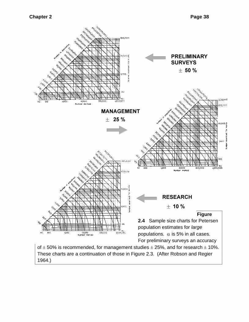
Chapter 2 Page 38
Figure
2.4 Sample size charts for Petersen
population estimates for large
populations. is 5% in all cases.
For preliminary surveys an accuracy
of 50% is recommended, for management studies 25%, and for research 10%.
These charts are a continuation of those in Figure 2.3. (After Robson and Regier
1964.)
Chapter 2 Page 39
The choice of which combination of marking (M) and capturing (C) will depend in part on
the ease of marking and ease of sampling for marked individuals. For example, it
may be very easy to mark individuals, but very difficult to recapture large samples.
In this situation in example 2 we might decide to take M = 92,000 and C = 400.
Alternatively, it may be very expensive to mark animals and cheap to recapture
them in large numbers, and we might take M = 7000 and C = 10,000 for the same
example. In normal circumstances we try to equalize sample sizes so M C, the
number marked is approximately the same as the number caught in the second
Petersen sample. This balance of M C is the point of minimum effort in terms of
numbers of animals that need to be handled to achieve a given level of precision.
I cannot overemphasize the importance of going through this sample size
estimation procedure before you start an ecological study which uses mark-
recapture. To obtain even moderate accuracy in population estimation it is often
necessary to mark 50% or more of the individuals in a population and the
information you can obtain from Figures 2.3 and 2.4 can tell you how much work you
must do and whether the project you are starting is feasible at all.
2.1.3 Assumptions of Petersen Method
For N̂ in formula (2.2) or (2.3) to be an accurate estimate of population size the
following five assumptions must hold:
1. The population is closed, so that N is constant.
2. All animals have the same chance of getting caught in the first sample.
3. Marking individuals does not affect their catchability.
4. Animals do not lose marks between the two sampling periods.
5. All marks are reported upon discovery in the second sample.
If the first assumption is to hold in a biological population, it is essential that the
Petersen method be applied over a short period of time. This is an important
consideration in experimental design because if a long period of sampling is needed
to get the size of sample required, the method may lose its precision.
There are several simple ways in which the first assumption can be violated
without affecting the validity of the Petersen estimate. If there are accidental deaths
during the first sampling and marking, the estimate of N is valid but refers to the
number of individuals alive in the population after the first sample is released.
Natural mortality may occur between the first and second Petersen samples without
affecting the estimation if marked and unmarked animals have an equal chance of
dying between the first and second samples. The question of whether mortality falls
equally on marked and unmarked animals is difficult to answer for any natural
population, and this assumption is best avoided if possible.
Population size (N) in a mark-recapture estimation always refers to the
catchable population, which may or may not be the entire population. For example,

Chapter 2 Page 40
nets will catch only fish above a certain size, and smaller individuals are thus
ignored in the Petersen calculations. The recruitment of young animals into the
catchable population between the first and second samples tends to decrease the
proportion of marked animals in the second sample and thus inflate the Petersen
estimate of N above the true population size at time one. When there is recruitment
but no mortality, N̂ will be a valid estimate of population size at the time of the
second sample. Fishery scientists have developed tests for recruitment and
subsequent corrections that can be applied to Petersen estimates when there is
recruitment (see Seber (1982), p. 72 ff.), but the best advice is still the simplest:
avoid recruitment of new individuals into the population by sampling over a short
time interval.
One of the crucial assumptions of mark-recapture work is that marked and
unmarked animals are equally catchable. This assumption is necessary for all the
methods discussed in this chapter and I defer discussion until later (page 000) on
methods for testing this assumption.
Random sampling is critical if we are to obtain accurate Petersen estimates,
but it is difficult to achieve in field programs. We cannot number all the animals in
the population and select randomly M individuals for marking and later C individuals
for capture. If all animals are equally catchable, we can approximate a random
sample by sampling areas at random with a constant effort. We can divide the total
area into equal subareas, and allot sampling effort to the subareas selected from a
random number table. All points selected must be sampled with the same effort.
Systematic sampling (Chapter 8, page 000) is often used in place of random
sampling. Systematic sampling will provide adequate estimates of population size
only if there is uniform mixing of marked and unmarked animals, and all individuals
are equally catchable. Uniform mixing is unlikely to be achieved in most animals
which show territorial behavior or well-defined home ranges. Where possible you
should aim for a random sample and avoid the dangerous assumption of uniform
mixing that must be made after systematic samples are taken.
I will not review here the various marking methods applied to animals and
plants. Seber (1982) and Sutherland (2006) give general references for marking
methods for fish, birds, mammals, and insects. Experienced field workers can offer
much practical advice on marking specific kinds of organisms, and not all of this
advice is contained in books. New metals, plastics, and dyes are constantly being
developed as well. The importance of these technological developments in marking
cannot be overemphasized because of the problems of lost marks and unreported
marks. Poor marking techniques will destroy the most carefully designed and
statistically perfect mark-recapture scheme, and it is important to use durable tags
that will not interfere with the animal's life cycle.

Chapter 2 Page 41
Tag losses can be estimated easily by giving all the M individuals in the first
Petersen sample two types of tags, and then by recording in the second sample:
RA = number of tagged animals in second sample with only an A type tag
(i.e. they have lost their B-tag)
RB = number of tagged animals in second sample with only a B type tag
(i.e. they have lost their A-tag)
RAB = number of tagged animals in second sample with both A and B
tags present.
Clearly, if RA and RB are both zero you are probably not having a tag loss problem. The
total number of recaptures is defined as
R = RA + RB + RAB + Number of individuals losing both tags
and thus being classed as unmarked
Seber (1982, p. 95) shows that, if we define:
( )( )
= A B
A AB B AB
R Rk
R R R R+ +
and
1 =
1c
k−
Then we can estimate the total number of recaptures as:
( )ˆ = A B ABR c R R R+ + (2.6)
For example, if we mark 500 beetles with dots of cellulose paint (A) and reflecting paint
(B) and obtain in the second sample:
RA = 23
RB = 6
RAB = 127
we obtain:
( ) ( )( ) ( )
23 6 = = 0.006917
23 127 6 127k
+ +
1 = = 1.00697
1 0.006917c
−
( )ˆ = 1.00697 23 6 127 = 157.09R + +

Chapter 2 Page 42
Thus we observe R = 156 and estimate R̂ = 157 so that only one insect is
estimated to have lost both marks during the experiment. From this type of
experiment we can calculate the probabilities of losing marks of a given type:
( )
Probability of losing a tag of Type A =
between samples one and twoB
B AB
R
R R
+ (2.7)
( )
Probability of losing a tag of Type B =
between samples one and twoA
A AB
R
R R
+ (2.8)
In this example the probability of losing a cellulose dot is only 0.045 but the chances of
losing a reflecting dot are 0.153, more than a three-fold difference between tag
types.
The failure to report all tags recovered may be important for species sampled
by hunting or commercial fishing in which the individuals recovering the tags are not
particularly interested in the data obtained. Tag returns are affected by the size of
the tag reward and the ease of visibility of the tags.
An array of radio- and satellite-collar methods can estimate tag loss for collars
directly. Musyl et al. (2011) have an excellent discussion of problems of satellite tag
loss in fishes and sea turtles and the statistical methods that can be used to deal
with tag loss estimation.
2.2 SCHNABEL METHOD
Schnabel (1938) extended the Petersen method to a series of samples in
which there is a 2nd, 3rd, 4th...nth sample. Individuals caught at each sample are first
examined for marks, then marked and released. Marking occurs in each of the
sampling times. Only a single type of mark need be used, since throughout a
Schnabel experiment we need to distinguish only two types of individuals: marked =
caught in one or more prior samples; and unmarked = never caught before. We
determine for each sample t:
Ct = total number of individuals caught in sample t
Rt = number of individuals already marked when caught in sample t
Ut = number of individuals marked for first time and released in sample t
Normally Ct = Rt + Ut
but if there are accidental deaths involving either marked or unmarked animals,
these are subtracted from the Ut value*. The number of marked individuals in the
population continues to accumulate as we add further samples, and we define:
* The number of accidental deaths is assumed to be small.
Chapter 2 Page 43
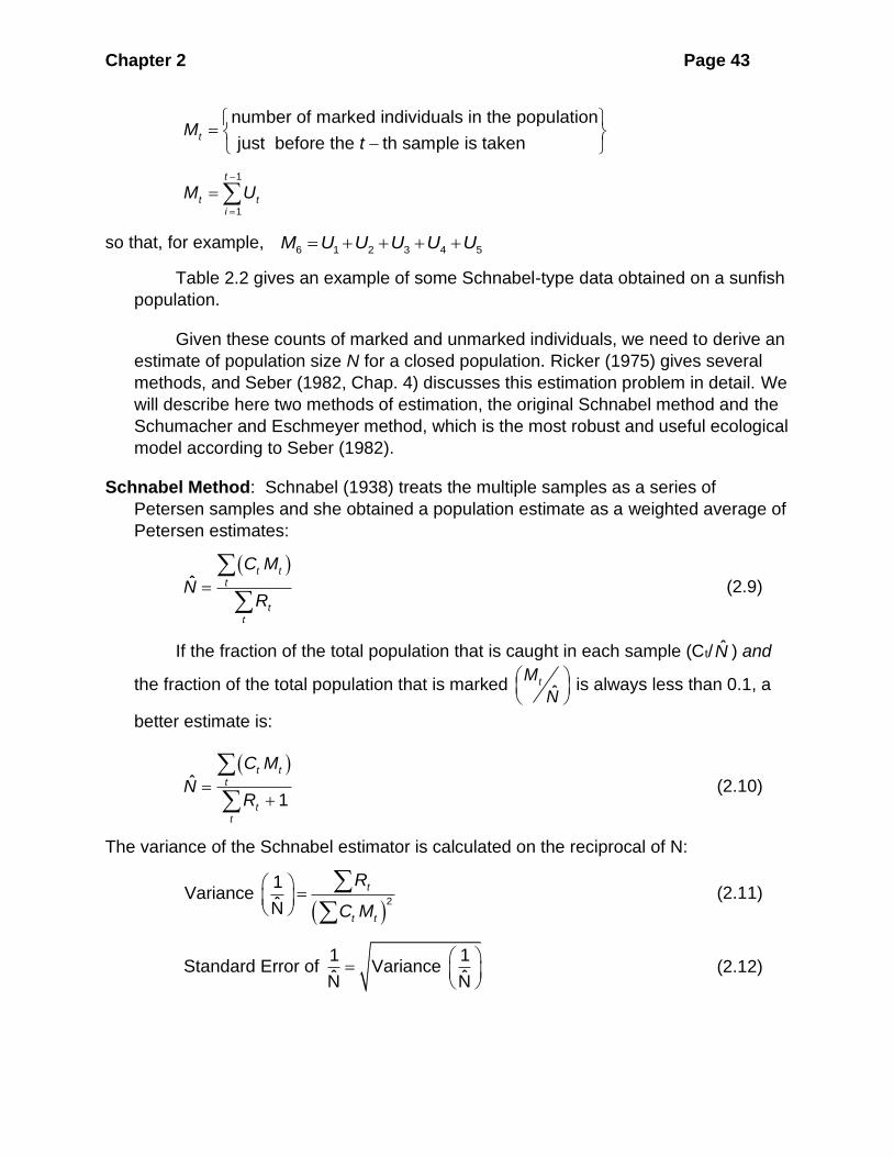
number of marked individuals in the population
just before the th sample is takentM
t
=
−
1
1
t
t t
i
M U−
=
=
so that, for example, 6 1 2 3 4 5M U U U U U= + + + +
Table 2.2 gives an example of some Schnabel-type data obtained on a sunfish
population.
Given these counts of marked and unmarked individuals, we need to derive an
estimate of population size N for a closed population. Ricker (1975) gives several
methods, and Seber (1982, Chap. 4) discusses this estimation problem in detail. We
will describe here two methods of estimation, the original Schnabel method and the
Schumacher and Eschmeyer method, which is the most robust and useful ecological
model according to Seber (1982).
Schnabel Method: Schnabel (1938) treats the multiple samples as a series of
Petersen samples and she obtained a population estimate as a weighted average of
Petersen estimates:
( )ˆ
t t
t
t
t
C M
NR
=
(2.9)
If the fraction of the total population that is caught in each sample (Ct/ N̂ ) and
the fraction of the total population that is marked ˆtM
N
is always less than 0.1, a
better estimate is:
( )ˆ
1
t t
t
t
t
C M
NR
=+
(2.10)
The variance of the Schnabel estimator is calculated on the reciprocal of N:
( )2
1Variance
N̂
t
t t
R
C M
=
(2.11)
1 1Standard Error of Variance
ˆ ˆN N
=
(2.12)
Chapter 2 Page 44
Schumacher and Eschmeyer Method: Schumacher and Eschmeyer (1943) pointed
out that if one plotted on arithmetic paper:
X-axis: Mt, number of individuals previously marked (before time t)
Y-axis: Rt/Ct, proportion of marked individuals in the t-th sample
the plotted points should lie on a straight line of slope (1/N) passing through the origin.
Thus one could use linear regression techniques to obtain an estimate of the slope
(1/N) and thus an estimate of population size. The appropriate formula of estimation
is:
( )
( )
2
1
1
ˆ
s
t t
t
s
t t
t
C M
N
R M
=
=
=
(2.13)
where s = total number of samples
The variance of Schumacher estimator is obtained from linear regression theory as the
variance of the slope of the regression (Zar 1996, p. 330; Sokal and Rohlf 1995, p.
471). In terms of mark-recapture data:
( )2
2
2
1Variance of
ˆ 2
t tt
t t t
R MRC C M
sN
−
= −
(2.14)
where s = number of samples included in the summations
The standard error of the slope of the regression is obtained as follows:
( )( )2
1Variance of ˆ1
Standard Error of ˆ
t t
N
N C M
=
(2.15)
2.2.1 Confidence Intervals for Schnabel Estimates
If the total number of recaptures ( tR ) is less than 50, confidence limits for the
Schnabel population estimate should be obtained from the Poisson distribution
(Table 2.1, page 30). These confidence limits for tR from Table 2.1 can be
substituted into equations (2.14) or (2.15) as the denominator, and the upper and
lower confidence limits for population size estimated.
For the Schnabel method if the total number of recaptures ( )tR is above 50,
use the normal approximation derived by Seber (1982, p. 142). This large-sample
Chapter 2 Page 45
procedure uses the standard error and a t-table to get confidence limits for ( )1N̂
as
follows:
1S.E.
ˆt
N (2.16)
where S.E. = standard error of 1/N (equation 2.12 or 2.15)
t = value from Student's t-table for (100 - )% confidence limits.
Enter the t-table with (s-1) degrees of freedom for the Schnabel method and (s-2)
degrees of freedom for the Schumacher and Eschmeyer methods, where s is the
number of samples. Invert these limits to obtain confidence limits for N̂ . Note that
this method (equation 2.16) is used for all Schumacher-Eschmeyer estimates,
regardless of the number of recaptures. This procedure is an approximation but the
confidence limits obtained are sufficiently accurate for all practical purposes.
We can use the data in Table 2.2 to illustrate both these calculations. From the
data in Table 2.2 we obtain:
Chapter 2 Page 46
TABLE 2.2 Mark-recapture data obtained for a Schnabel-type estimate of population
size
Date, t Number of
fish
caught
Ct
Number of
recapturesb
Rt
Number newly
marked
(less
deaths)c
Marked fish at
larged
Mt
June 2 10 0 10 0
June 3 27 0 27 10
June 4 17 0 17 37
June 5 7 0 7 54
June 6 1 0 1 61
June 7 5 0 5 62
June 8 6 2 4 67
June 9 15 1 14 71
June 10 9 5 4 85
June 11 18 5 13 89
June 12 16 4 10 102
June 13 5 2 3 112
June 14 7 2 4 115
June 15
19 3 - 119
Totals 162 24 119 984
a S.D. Gerking (1953) marked and released sunfish in an Indiana lake for 14
days and obtained these data.
b The number of fish already marked when taken from the nets.
c Note that there were two accidental deaths on June 12 and one death on June
14.
d Number of marked fish assumed to be alive in the lake in the instant just before
sample t is taken.

Chapter 2 Page 47
t tC M = 10,740
( )2
t tC M .= 970,296
t tR M .= 2294
2
t
t
RC
.= 7.7452
For the Schnabel estimator, from equation (2.9)
10,740ˆ 447.5 sunfish24
N = =
A 95% confidence interval for this estimate is obtained from the Poisson distribution
because there are only 24 recaptures. From Table 2.1 with tR = 24 recaptures,
the 95% confidence limits on tR are 14.921 and 34.665. Using equation (2.9)
with these limits we obtain:
( ) 10,740Lower 95% confidence limit = 309.8
34.665
t t
t
C M
R= =
( ) 10,740Upper 95% confidence limit = 719.8 sunfish
14.921
t t
t
C M
R= =
The 95% confidence limits for the Schnabel population estimate are 310 to 720 for the
data in Table 2.1.
For the Schumacher-Eschmeyer estimator, from equation (2.13):
970,296ˆ 423 sunfish2294
N = =
The variance of this estimate, from equation (2.14), is:
( )2
22947.7452
970,2961Variance of 0.1934719
ˆ 14 2N
− = =
−
1 0.1934719Standard error 0.0004465364
ˆ 970,296N
= =
The confidence interval from equation (2.16) is:
( )( )1
2.179 0.0004465364423
Chapter 2 Page 48
or 0.0013912 to 0.0033372. Taking reciprocals, the 95% confidence limits for the
Schumacher-Eschmeyer estimator are 300 and 719 sunfish, very similar to those
obtained from the Schnable method.
Seber (1982) recommends the Schumacher-Eschmeyer estimator as the most
robust and useful one for multiple censuses on closed populations. Program RECAP
(Appendix 2, page 000) computes both these estimates and their appropriate
confidence intervals. Box 2.2 illustrates an example of the use of the Schumacher-
Eschmeyer estimator.
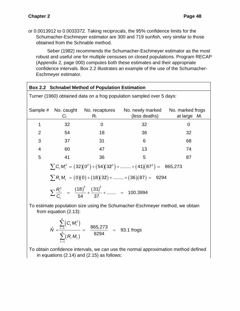
Box 2.2 Schnabel Method of Population Estimation
Turner (1960) obtained data on a frog population sampled over 5 days:
Sample # No. caught
Ct
No. recaptures
Rt
No. newly marked
(less deaths)
No. marked frogs
at large Mt
1 32 0 32 0
2 54 18 36 32
3 37 31 6 68
4 60 47 13 74
5 41 36 5 87
( )( ) ( )( ) ( )( )2 2 2 232 0 54 32 ........ 41 87 865,273t tC M = + + + =
( )( ) ( )( ) ( )( )0 0 18 32 ........ 36 87 9294t tR M = + + + =
( ) ( )2 22 18 31
....... 100.399454 37
t
t
R
C= + + =
To estimate population size using the Schumacher-Eschmeyer method, we obtain
from equation (2.13):
( )
( )
2
1
1
865,273ˆ 93.1 frogs9294
s
t t
t
s
t t
t
C M
N
R M
=
=
= = =
To obtain confidence intervals, we can use the normal approximation method defined
in equations (2.14) and (2.15) as follows:
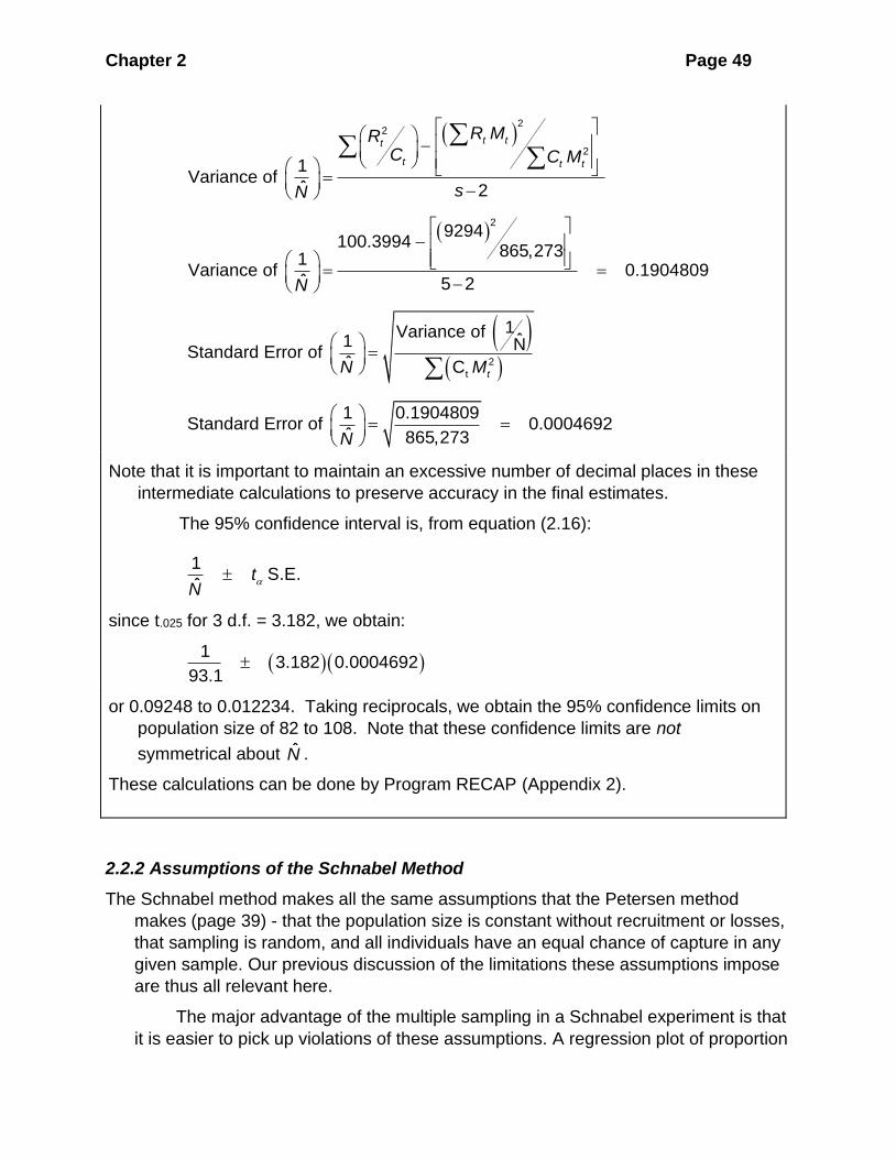
Chapter 2 Page 49
( )2
2
2
1Variance of
ˆ 2
t tt
t t t
R MRC C M
sN
−
= −
( )2
9294100.3994
865,2731Variance of 0.1904809
ˆ 5 2N
− = =
−
( )( )2
t
1Variance of ˆ1 NStandard Error of
ˆ C tN M
=
1 0.1904809Standard Error of 0.0004692
ˆ 865,273N
= =
Note that it is important to maintain an excessive number of decimal places in these
intermediate calculations to preserve accuracy in the final estimates.
The 95% confidence interval is, from equation (2.16):
1S.E.
ˆt
N
since t.025 for 3 d.f. = 3.182, we obtain:
( )( )1
3.182 0.000469293.1
or 0.09248 to 0.012234. Taking reciprocals, we obtain the 95% confidence limits on
population size of 82 to 108. Note that these confidence limits are not
symmetrical about N̂ .
These calculations can be done by Program RECAP (Appendix 2).
2.2.2 Assumptions of the Schnabel Method
The Schnabel method makes all the same assumptions that the Petersen method
makes (page 39) - that the population size is constant without recruitment or losses,
that sampling is random, and all individuals have an equal chance of capture in any
given sample. Our previous discussion of the limitations these assumptions impose
are thus all relevant here.
The major advantage of the multiple sampling in a Schnabel experiment is that
it is easier to pick up violations of these assumptions. A regression plot of proportion
Chapter 2 Page 50
of marked animals (Y) on number previously marked (X) will be linear if these
assumptions are true, but will become curved when the assumptions are violated.
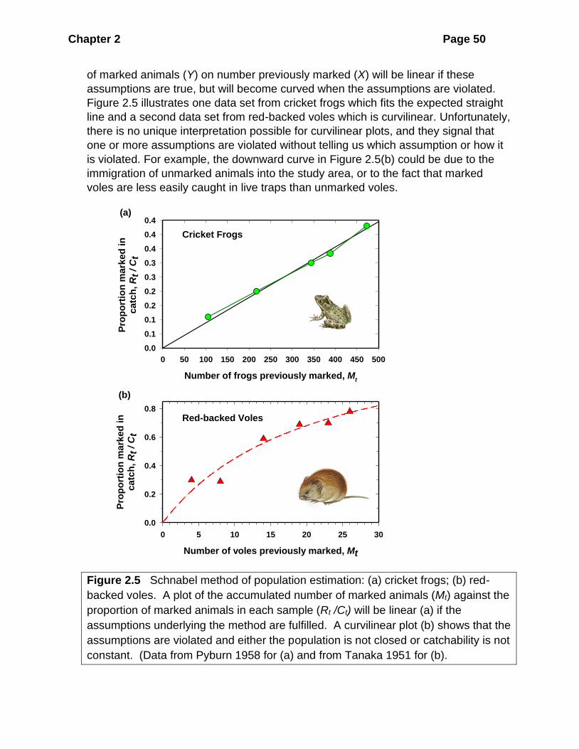
Figure 2.5 illustrates one data set from cricket frogs which fits the expected straight
line and a second data set from red-backed voles which is curvilinear. Unfortunately,
there is no unique interpretation possible for curvilinear plots, and they signal that
one or more assumptions are violated without telling us which assumption or how it
is violated. For example, the downward curve in Figure 2.5(b) could be due to the
immigration of unmarked animals into the study area, or to the fact that marked
voles are less easily caught in live traps than unmarked voles.
Figure 2.5 Schnabel method of population estimation: (a) cricket frogs; (b) red-
backed voles. A plot of the accumulated number of marked animals (Mt) against the
proportion of marked animals in each sample (Rt /Ct) will be linear (a) if the
assumptions underlying the method are fulfilled. A curvilinear plot (b) shows that the
assumptions are violated and either the population is not closed or catchability is not
constant. (Data from Pyburn 1958 for (a) and from Tanaka 1951 for (b).
Cricket Frogs
Number of frogs previously marked, Mt
0 50 100 150 200 250 300 350 400 450 500
Pro
po
rtio
n m
ark
ed
in
ca
tch
, R
t / C
t
0.0
0.1
0.1
0.2
0.2
0.3
0.3
0.4
0.4
0.4
Red-backed Voles
Number of voles previously marked, Mt
0 5 10 15 20 25 30
Pro
po
rtio
n m
ark
ed
in
ca
tch
, R
t / C
t
0.0
0.2
0.4
0.6
0.8
(a)
(b)

Chapter 2 Page 51
When a curvilinear relationship is present, you may still be able to obtain a
population estimate by the use of Tanaka's model (see Seber, 1982, p. 145). The
procedure is to plot on log-log paper:
X-axis: tM (number marked at large)
Y-axis: t
t
CR
(number caught / number of recaptures)
Figure 2.6 shows this graph for the same vole data plotted in Figure 2.5(b).
Figure 2.6 Tanaka’s model of population estimation: red-backed voles. A log-log
plot of the number of marked animals at large (Mt) against the ratio of total catch to
marked catch (Ct /Rt) should be a straight line to fit this model, and the x-intercept
(arrow) is the estimate of population size. These data are the same as those plotted
in Figure 2.5b. (Data from Tanaka 1951.)
If Tanaka's model is applicable, this log-log plot should be a straight line, and the X-
intercept is an estimate of population size. Thus, as a first approximation a visual
estimate of N can be made by drawing the regression line by eye and obtaining the
X-axis intercept, as shown in Figure 2.6. The actual formulae for calculating N̂ by
the Tanaka method are given in Seber (1982, p. 147) and are not repeated here.
The Schnabel and Tanaka methods both assume that the number of
accidental deaths or removals is negligible so that population size is constant. If a
substantial fraction of the samples is removed from the population, for example by
hunting or commercial fishing, corrections to the population estimates given above
Red-backed Voles
Number of voles previously marked, Mt (log scale)
4 6 8 10 20 30 40 50
Ra
tio
of
tota
l c
atc
h t
o m
ark
ed
an
ima
ls
Ct
/Rt
(lo
g s
ca
le)
1
1.5
2
3
4

Chapter 2 Page 52
should be applied. Seber (1982, p. 152) provides details of how to correct these
estimates for known removals.
2.3 PROGRAM CAPTURE AND PROGRAM MARK
The simple approaches to estimating population size typified by the Petersen
and Schnabel methods have been superseded by more complex methods that are
computer intensive. I have detailed the procedures in the Petersen and Schnabel
methods to introduce you to some of the problems of estimation with mark-recapture
data. In reality if you wish to use these methods you must utilize Program
CAPTURE (Otis et al. 1978) or Program MARK (White 2008, Cooch and White
2010). We begin with Program CAPTURE.
Simple models for closed populations like the Petersen Method may fail
because of two assumptions that are critical for estimation:
1. All animals have the same chance of getting caught in all the samples.
2. Marking individuals does not affect their catchability in later samples
Otis et al. (1978) set out an array of models in Program CAPTURE that take into
account some of the simpler aspects of unequal catchability. These methods
complement the Petersen and Schnabel estimators discussed above for closed
populations but they are more restrictive because all the methods in Program
CAPTURE assume that every marked animal can be individually recognized and at
least three sampling periods were used. These methods are all computer-intensive
1. They involve more complex mathematics than we can discuss here in detail and I
will cover only the basic outline of these methods and indicate the data needed for
these calculations.
The simplest form of data input is in the form of an X Matrix. The rows of this
matrix represent the individual animals that were captured in the study, and the
columns of the matrix represent the time periods of capture. In each column a 0
(zero) indicates that the individual in question was not caught during this sampling
time, and a 1 (one) indicates that the individual was captured. A sample X matrix for
7 capture times is as follows:
3455 1 0 0 1 1 1 0
3456 1 1 1 0 0 0 1
3458 1 0 0 0 0 0 0
1 These programs are currently available from Colorado State University at
www.cnr.colostate.edu/~gwhite/software.html.
Tag number Time 1 Time 2 Time 3 Time 4 Time5 Time 6 Time 7
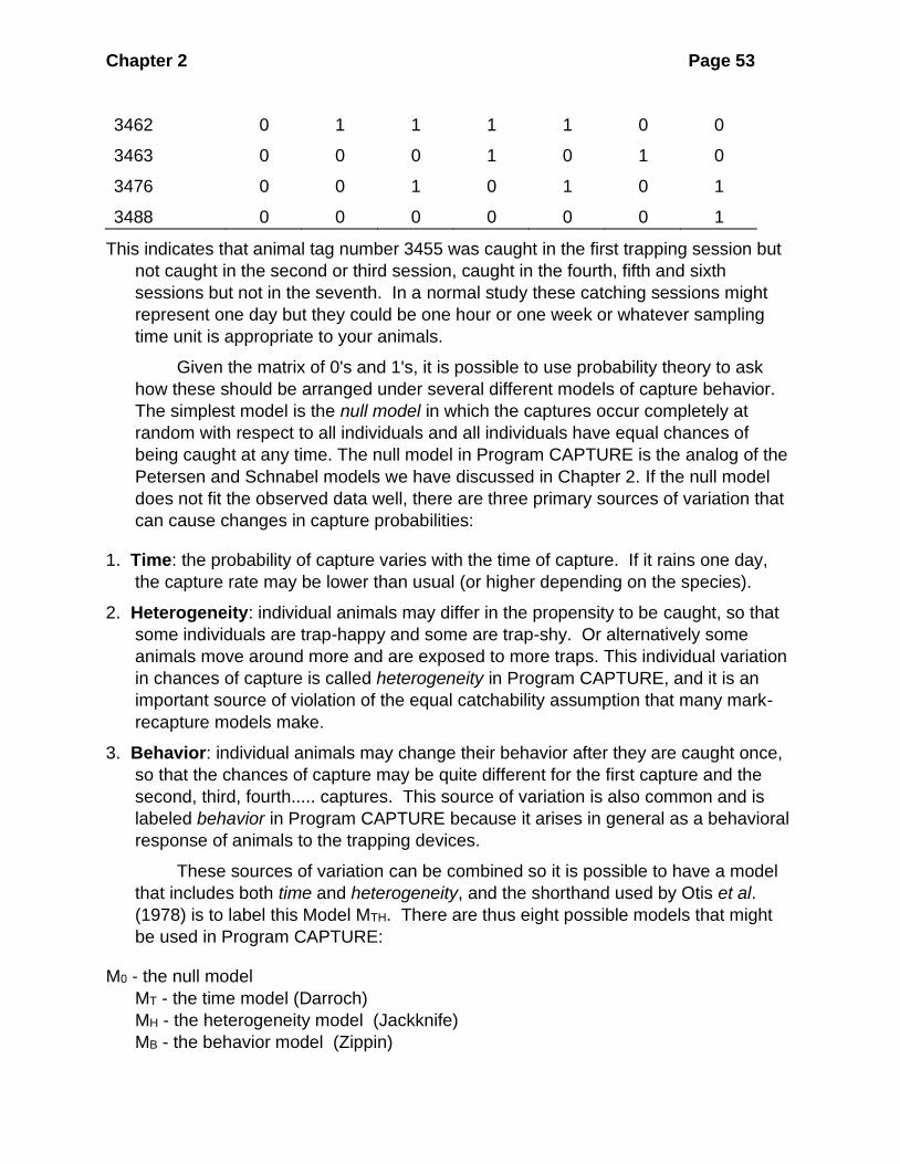
Chapter 2 Page 53
3462 0 1 1 1 1 0 0
3463 0 0 0 1 0 1 0
3476 0 0 1 0 1 0 1
3488 0 0 0 0 0 0 1
This indicates that animal tag number 3455 was caught in the first trapping session but
not caught in the second or third session, caught in the fourth, fifth and sixth
sessions but not in the seventh. In a normal study these catching sessions might
represent one day but they could be one hour or one week or whatever sampling
time unit is appropriate to your animals.
Given the matrix of 0's and 1's, it is possible to use probability theory to ask
how these should be arranged under several different models of capture behavior.
The simplest model is the null model in which the captures occur completely at
random with respect to all individuals and all individuals have equal chances of
being caught at any time. The null model in Program CAPTURE is the analog of the
Petersen and Schnabel models we have discussed in Chapter 2. If the null model
does not fit the observed data well, there are three primary sources of variation that
can cause changes in capture probabilities:
1. Time: the probability of capture varies with the time of capture. If it rains one day,
the capture rate may be lower than usual (or higher depending on the species).
2. Heterogeneity: individual animals may differ in the propensity to be caught, so that
some individuals are trap-happy and some are trap-shy. Or alternatively some
animals move around more and are exposed to more traps. This individual variation
in chances of capture is called heterogeneity in Program CAPTURE, and it is an
important source of violation of the equal catchability assumption that many mark-
recapture models make.
3. Behavior: individual animals may change their behavior after they are caught once,
so that the chances of capture may be quite different for the first capture and the
second, third, fourth..... captures. This source of variation is also common and is
labeled behavior in Program CAPTURE because it arises in general as a behavioral
response of animals to the trapping devices.
These sources of variation can be combined so it is possible to have a model
that includes both time and heterogeneity, and the shorthand used by Otis et al.
(1978) is to label this Model MTH. There are thus eight possible models that might
be used in Program CAPTURE:
M0 - the null model
MT - the time model (Darroch)
MH - the heterogeneity model (Jackknife)
MB - the behavior model (Zippin)

Chapter 2 Page 54
MTH - the time and heterogeneity model
MTB - the time and behavior model
MBH - the behavior and heterogeneity model (Generalized Removal)
MTBH - the full model with time, heterogeneity, and behavior varying
The more complicated models as you might guess are harder to fit to observed data.
The key problem remaining is which of these models to use on your particular
data. Otis et al. (1978) have devised a series of chi-squared tests to assist in this
choice, but these do not give a unique answer with most data sets. Work is
continuing in this area to try to develop better methods of model selection. Program
MARK has a model-selection routine that operates for the comparison of some
models that use maximum likelihood methods.
The details of the models and the calculations are presented in Otis et al.
(1978) and for ecologists a general description of the procedures used and some
sample data runs are given in Amstrup et al. (2006). Maximum-likelihood methods
(see Chapter 3 for an example) are used in many of the estimation procedures in
CAPTURE, and I will illustrate only one method here, the null model M0. The best
estimate of N̂ for model M0 is obtained from the following maximum likelihood
equation:
( )( )
( ) ( ) ( ) ( ) ( ) ( )0
!ˆ ˆ, X ln ln ln ln!
NL N p n n t N n t N n t N t N
N M
= + + − − − −
(2.17)
where 0N̂ = estimated population size from the null model of CAPTURE
N = provisional estimate of population size
p̂ = probability of capture
M = total number of different individuals captured in the entire sampling
period
n = total number of captures during the entire sampling period
t = number of samples (e.g. days)
ln = natural log (loge)
L = log likelihood of the estimated value 0N̂ and p, given the observed X
matrix of captures
This equation is solved by trial and error to determine the value of N that maximizes the
log likelihood (as in Figure 3.5), and this value of N is the best estimate of
population size 0N̂ .
Once the value of 0N̂ has been determined, the probability of capture can be obtained
from:

Chapter 2 Page 55
0
ˆˆ
np
t N= (2.18)
where all terms are as defined above. The variance of the estimated population size is
obtained from:
( )( ) ( )
00
ˆˆ ˆ
ˆ ˆ1 1 1t
NVar N
p t p t−
=− − − + −
(2.19)
The standard error of this population estimate is the square root of this variance, and
hence the confidence limits for the estimated population size are given by the usual
formula:
( )0 0ˆ ˆ ˆN z Var N (2.20)
where z = standard normal deviate (i.e. 1.960 for 95% confidence limits, 2.576 for
99% limits, or 1.645 for 90% limits).
Because these confidence limits are based on the normal distribution, there is
a tendency for confidence intervals of population estimates to be narrower than they
ought to be (Otis et al. 1978, p. 105).
The null model M0 has a simple form when there are only two sampling periods
(as in a Petersen sample). For this situation equation (2.17) simplifies to:
( ) 2
1 2
0ˆ
4
n nN
m
+= (3.24)
where n1 = number of individuals captured in the first sample and marked
n2 = number of individuals captured in the second sample
m = number of recaptured individuals in the second sample
For example, from the data in Box 2.1 (page 000) the null model estimate of population
size is:
( ) ( )( )
22
1 2
0
948 421ˆ 2806 hares4 4 167
n nN
m
+ += = =
This estimate is 18% higher than the Petersen estimate of 2383 calculated in Box 2.1.
The null model tends to be biased towards overestimation when the number of
sampling times (t) is less than 5, unless the proportion of marked animals is
relatively high. For this reason the Petersen method is recommended for data
gathered over two sampling periods, as in this example. Program CAPTURE and
Program MARK become most useful when there are at least 4-5 sampling times in
the mark-recapture data, and like all mark-recapture estimators they provide better
estimates when a high fraction of the population is marked.

Chapter 2 Page 56
Box 2.3 gives a sample set of calculations for the null model from Program
CAPTURE.
Chapter 2 Page 57
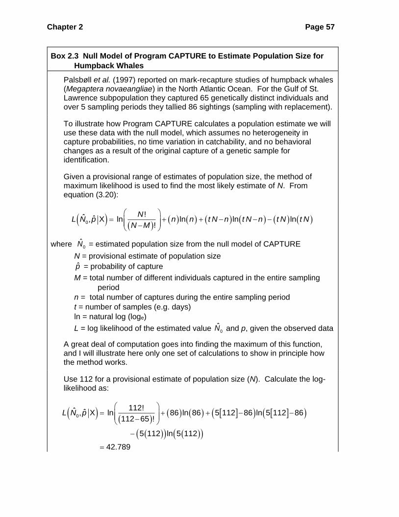
Box 2.3 Null Model of Program CAPTURE to Estimate Population Size for
Humpback Whales
Palsbøll et al. (1997) reported on mark-recapture studies of humpback whales (Megaptera novaeangliae) in the North Atlantic Ocean. For the Gulf of St. Lawrence subpopulation they captured 65 genetically distinct individuals and over 5 sampling periods they tallied 86 sightings (sampling with replacement).
To illustrate how Program CAPTURE calculates a population estimate we will use these data with the null model, which assumes no heterogeneity in capture probabilities, no time variation in catchability, and no behavioral changes as a result of the original capture of a genetic sample for identification.
Given a provisional range of estimates of population size, the method of maximum likelihood is used to find the most likely estimate of N. From equation (3.20):
( )( )
( ) ( ) ( ) ( ) ( ) ( )0
!ˆ ˆ, X ln ln ln ln!
NL N p n n t N n t N n t N t N
N M
= + + − − − −
where 0N̂ = estimated population size from the null model of CAPTURE
N = provisional estimate of population size
p̂ = probability of capture
M = total number of different individuals captured in the entire sampling
period
n = total number of captures during the entire sampling period
t = number of samples (e.g. days)
ln = natural log (loge)
L = log likelihood of the estimated value 0N̂ and p, given the observed data
A great deal of computation goes into finding the maximum of this function, and I will illustrate here only one set of calculations to show in principle how the method works.
Use 112 for a provisional estimate of population size (N). Calculate the log-likelihood as:
( )( )
( ) ( ) ( ) ( )
( )( ) ( )( )
0
112!ˆ ˆ, X ln 86 ln 86 5 112 86 ln 5 112 86112 65 !
5 112 ln 5 112
42.789
L N p
= + + − − −
−
=

Chapter 2 Page 58
By repeating this calculation for other provisional estimates of N you can
determine:
( )
( )
( )
0
0
0
ˆ ˆfor 117, , 42.885
ˆ ˆfor 121, , 42.904
ˆ ˆfor 126, , 42.868
N L N p X
N L N p X
N L N p X
= =
= =
= =
and the maximum likelihood occurs at N̂ of 121 whales.
Note that in practice you would use Program CAPTURE to do these calculations and also to test whether more complex models involving variation in probability of capture due to time or behavior might be present in these data.
The probability of an individual whale being sighted and sampled for DNA at any given sample period can be determined from equation (3.21):
( )0
86ˆ 0.142
ˆ 5 121
np
t N= = =
Given this probability we can now estimate the variance of population size from equation (3.22)
( )( ) ( )
( ) ( )
00
5
ˆˆ ˆ
ˆ ˆ1 1 1
121373.5
51 0.142 5 11 0.142
t
NVar N
p t p t−
−
=− − − + −
= =
− − + − −
and the resulting 90% confidence interval from equation (3.23) is:
( )0 0ˆ ˆ ˆ
121 1.645 373.5 or 121 32
N z Var N
These calculations including confidence limits can be done by Program CAPTURE or Program MARK and these methods are discussed in detail by Cooch and White (2010).
Program MARK is a very complex model for mark-recapture analysis and if
you are involved in mark-recapture research it will repay the large investment you
need to put into learning how to use it. It is currently the gold standard for mark-
recapture analysis. Program CAPTURE is much simpler to understand but cannot

Chapter 2 Page 59
do the elegant analyses implemented in Program MARK. Box 2.4 illustrates a data
set for snowshoe hares and the resulting CAPTURE estimates.
Box 2.4 Use of Program CAPTURE to Estimate Population Size for
Snowshoe Hares
Krebs et al. (2001) obtained these data from live trapping of snowshoe hares on a 25 ha grid in the Yukon in 2004. The data are summarized in an X-matrix format. The first number is the ear tag number of the individual, and the 1 and 0 indicate whether or not it was captured in session 1, 2, 3, or 4. For example, hare 2045 was captured only in session 4.
2153 1111 2154 1101 2155 1100 2035 1101 2039 1101 2040 1001 2041 1000 2207 1111 2205 1110 2208 1100 2084 1101 2210 1101 2211 1001 2083 1100 2218 0111 2042 0111 2043 0101 2045 0001
The first estimates CAPTURE provides is of the probable model which has the best fit to the data. For these data the program gives:
Model selection criteria. Model selected has maximum value.
Model M(o) M(h) M(b) M(bh) M(t) M(th) M(tb) M(tbh)
Criteria 0.14 0.00 0.09 0.15 0.91 1.00 0.45 0.34
The best model appears to be MTH, followed closely by MT
To illustrate Program CAPTURE estimates we calculated population estimates for all the models available using the format for data in CAPTURE.
The results of the computer run were the following estimates of N̂ for these 18 hares:
Chapter 2 Page 60
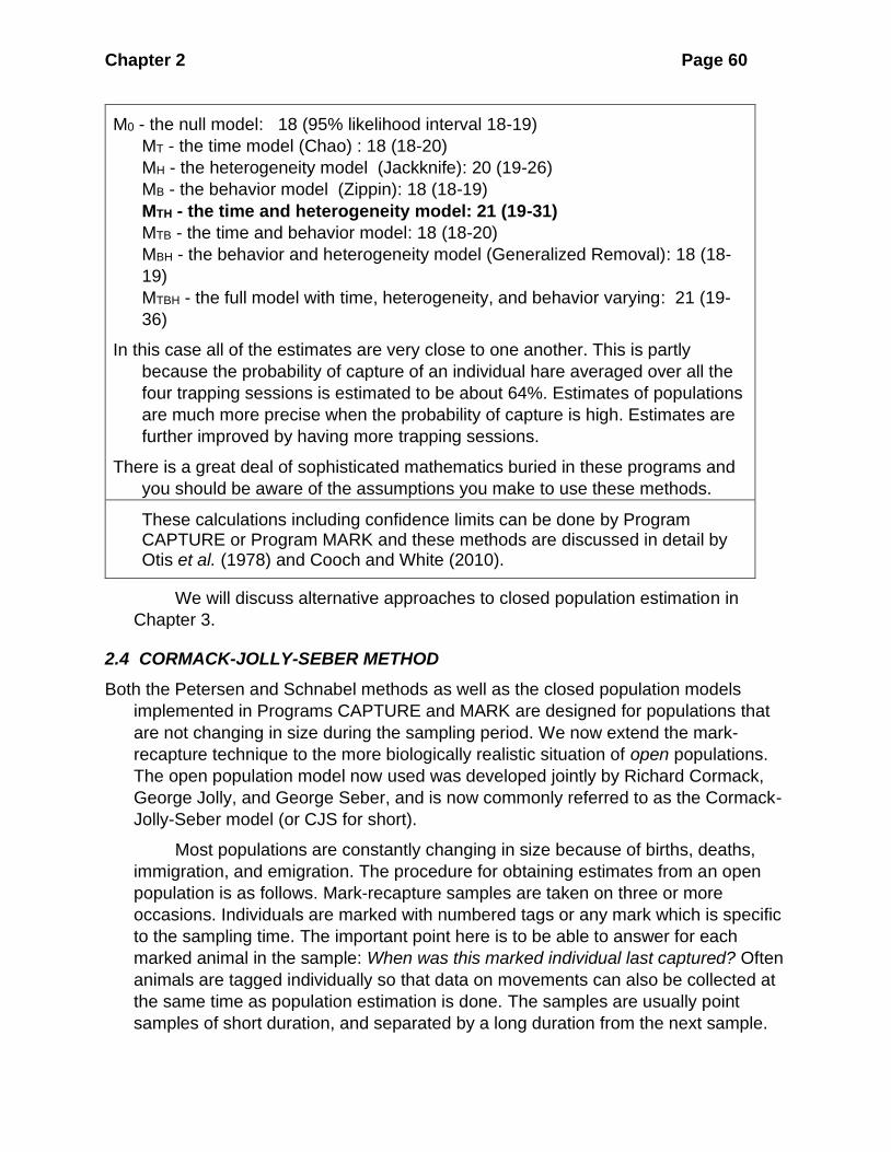
M0 - the null model: 18 (95% likelihood interval 18-19)
MT - the time model (Chao) : 18 (18-20)
MH - the heterogeneity model (Jackknife): 20 (19-26)
MB - the behavior model (Zippin): 18 (18-19)
MTH - the time and heterogeneity model: 21 (19-31)
MTB - the time and behavior model: 18 (18-20)
MBH - the behavior and heterogeneity model (Generalized Removal): 18 (18-
19)
MTBH - the full model with time, heterogeneity, and behavior varying: 21 (19-
36)
In this case all of the estimates are very close to one another. This is partly
because the probability of capture of an individual hare averaged over all the
four trapping sessions is estimated to be about 64%. Estimates of populations
are much more precise when the probability of capture is high. Estimates are
further improved by having more trapping sessions.
There is a great deal of sophisticated mathematics buried in these programs and
you should be aware of the assumptions you make to use these methods.
These calculations including confidence limits can be done by Program CAPTURE or Program MARK and these methods are discussed in detail by Otis et al. (1978) and Cooch and White (2010).
We will discuss alternative approaches to closed population estimation in
Chapter 3.
2.4 CORMACK-JOLLY-SEBER METHOD
Both the Petersen and Schnabel methods as well as the closed population models
implemented in Programs CAPTURE and MARK are designed for populations that
are not changing in size during the sampling period. We now extend the mark-
recapture technique to the more biologically realistic situation of open populations.
The open population model now used was developed jointly by Richard Cormack,
George Jolly, and George Seber, and is now commonly referred to as the Cormack-
Jolly-Seber model (or CJS for short).
Most populations are constantly changing in size because of births, deaths,
immigration, and emigration. The procedure for obtaining estimates from an open
population is as follows. Mark-recapture samples are taken on three or more
occasions. Individuals are marked with numbered tags or any mark which is specific
to the sampling time. The important point here is to be able to answer for each
marked animal in the sample: When was this marked individual last captured? Often
animals are tagged individually so that data on movements can also be collected at
the same time as population estimation is done. The samples are usually point
samples of short duration, and separated by a long duration from the next sample.
Chapter 2 Page 61
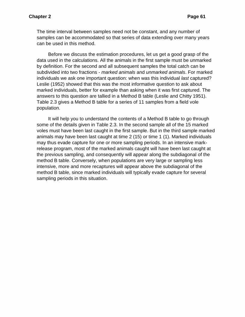
The time interval between samples need not be constant, and any number of
samples can be accommodated so that series of data extending over many years
can be used in this method.
Before we discuss the estimation procedures, let us get a good grasp of the
data used in the calculations. All the animals in the first sample must be unmarked
by definition. For the second and all subsequent samples the total catch can be
subdivided into two fractions - marked animals and unmarked animals. For marked
individuals we ask one important question: when was this individual last captured?
Leslie (1952) showed that this was the most informative question to ask about
marked individuals, better for example than asking when it was first captured. The
answers to this question are tallied in a Method B table (Leslie and Chitty 1951).
Table 2.3 gives a Method B table for a series of 11 samples from a field vole
population.
It will help you to understand the contents of a Method B table to go through
some of the details given in Table 2.3. In the second sample all of the 15 marked
voles must have been last caught in the first sample. But in the third sample marked
animals may have been last caught at time 2 (15) or time 1 (1). Marked individuals
may thus evade capture for one or more sampling periods. In an intensive mark-
release program, most of the marked animals caught will have been last caught at
the previous sampling, and consequently will appear along the subdiagonal of the
method B table. Conversely, when populations are very large or sampling less
intensive, more and more recaptures will appear above the subdiagonal of the
method B table, since marked individuals will typically evade capture for several
sampling periods in this situation.
Chapter 2 Page 62
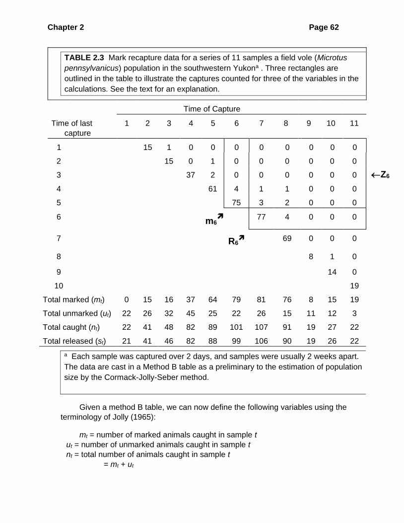
TABLE 2.3 Mark recapture data for a series of 11 samples a field vole (Microtus
pennsylvanicus) population in the southwestern Yukona . Three rectangles are
outlined in the table to illustrate the captures counted for three of the variables in the
calculations. See the text for an explanation.
Time of Capture
Time of last
capture
1 2 3 4 5 6 7 8 9 10 11
1 15 1 0 0 0 0 0 0 0 0
2 15 0 1 0 0 0 0 0 0
3 37 2 0 0 0 0 0 0
4 61 4 1 1 0 0 0
5 75 3 2 0 0 0
6 m6
77 4 0 0 0
7 R6
69 0 0 0
8 8 1 0
9 14 0
10 19
Total marked (mt) 0 15 16 37 64 79 81 76 8 15 19
Total unmarked (ut) 22 26 32 45 25 22 26 15 11 12 3
Total caught (nt) 22 41 48 82 89 101 107 91 19 27 22
Total released (st) 21 41 46 82 88 99 106 90 19 26 22
a Each sample was captured over 2 days, and samples were usually 2 weeks apart.
The data are cast in a Method B table as a preliminary to the estimation of population
size by the Cormack-Jolly-Seber method.
Given a method B table, we can now define the following variables using the
terminology of Jolly (1965):
mt = number of marked animals caught in sample t
ut = number of unmarked animals caught in sample t
nt = total number of animals caught in sample t
= mt + ut
Z6

Chapter 2 Page 63
st = total number of animals released after sample t
= (nt - accidental deaths or removals)
mrt = number of marked animals caught in sample t last caught in sample r
All these variables are symbols for the data written in the method B table. For example,
Table 2.3 shows that
m6 = 75 + 4 + 0 + 0 + 0 = 79 voles
We require two more variables for our calculations,
Rt = number of the st individuals released at sample t and caught again in some
later sample
Zt = number of individuals marked before sample t, not caught in sample t, but
caught in some sample after sample t
These last two variables are more easily visualized than described (see the rectangles
in Table 2.3). For example, as shown in the table, R6 =
77 + 4 + 0 + 0 + 0 = 81 voles
The Zt are those animals that missed getting caught in sample t, and survived to
turn up later on. In an intensive mark-release program, the Zt values will approach
zero. In this table for example
Z6 = 3 + 2 + 1 + 1 = 7 individuals
We can now proceed to estimate population size following Jolly (1965) from the simple
relationship:
Size of marked populationPopulation size =
Proportion of animals marked
The proportion of animals marked is estimated as:
1ˆ
1t
t
t
m
n
+=
+ (2.17)
where the "+ 1" is a correction for bias in small samples (Seber 1982, p. 204). The size
of the marked population is more difficult to estimate because there are two
components of the marked population at any sampling time: (1) marked animals
actually caught; and (2) marked animals present but not captured in sample t. Seber
(1982) showed that the sizes of the marked population could be estimated by:
( )1ˆ1
t t
t t
t
s ZM m
R
+= +
+ (2.18)
where tM = estimated size of the marked population just before sample time t
We can now estimate population size:
Chapter 2 Page 64
ˆˆ
ˆt
t
t
MN
= (2.19)
where ˆtN = estimated population size just before sample time t
Table 2.4 gives these estimates for the data in Table 2.3, and a few sample calculations
follow:
5
64 1ˆ 0.7222
89 1
+= =
+
6
79 1ˆ 0.7843
101 1
+= =
+
( )( )2
41 1 1ˆ 15 17.47
16 1M
+= + =
+
( )( )6
99 1 7ˆ 79 87.54
81 1M
+= + =
+
= =6
87.54ˆ 111.60.7843
N
We can derive an additional bonus from the use of the Cormack-Jolly-Seber
Model of population estimation - an estimate of the loss rate and the addition rate of
the population. Consider first the loss rate. We define
probability of surviving from sample time to sample time + 1
Size of marked population at start of sample time + 1=
Size of marked population at end of sample time
t t t
t
t
=
The marked population is added to during each sampling time as new individuals are
marked and released. Thus the size of the marked population at the end of sample t
consists of the marked individuals alive at the start of t plus the new individuals
marked during sampling time t, or in the symbols defined above:
( )1
ˆˆ
ˆt
t
t t t
M
M s m
+ =
+ − (2.20)
This formula corrects for all accidental deaths or removals at time t. Note that the
probability of surviving is determined by sampling the marked population only.
Survival in this context means staying alive on the study area. Individuals which
emigrate are counted as losses in the same way as individuals that die.

Chapter 2 Page 65
An addition rate to the population is called the dilution rate*, since it includes
both additions by births and by immigration:
dilution rate from sample time to sample time +1
Actual population size at sample time + 1
Expected populations size at sample time 1 if no additions occurred
t t t
t
t
=
=+
The expected population size in the absence of any gains is clearly:
Expected population Probability of survival Population size
size at time + 1 from to + 1 at time t t t t
=
and once we correct for accidental deaths we obtain:
( )1
ˆˆ
ˆˆ
t
t
t t t t
N
N n s
+=
− −
(2.21)
Thus if there are no additions at all, we expect the dilution rate to be 1.0, its theoretical
minimum value.
From a series of population estimates we can define:
1Finite rate of population change =
t
t
N
N
+
if there are no accidental deaths at time t. By rearranging formula (2.21) we see for the
ideal case of no accidental losses ( )t tn s= :
1Finite rate of population change
t
t t
t
N
N
+ = = (2.22)
Thus when there are no losses (t = 1.0) and no additions (
t = 1.0) the population
remains constant.
The addition rate to the population can also be expressed as a number of
individuals: If we define
* Note that the dilution rate defined here follows Jolly (1965) and differs from that of Leslie et al. (1953) {#4801}who defined a dilution factor that is zero when there is no dilution.
Chapter 2 Page 66
( )1
Number of new animals joining the population between
time and +1 still alive at time +1
ˆ ˆ ˆˆ
t
t t t t t t
Bt t and t
B N N n s+
=
= − − −
(2.23)
and this formula is clearly just a rearrangement of formula (2.21).
It is important to keep in mind that these estimates of , , , and tt t tN B are
not independent estimates of what is happening in a population, but they are all
interconnected so that when one estimate is poor they are all poor.
Estimates of population size (1N ) and dilution rate (
1 ) cannot be obtained for
the first sample, nor can any of these parameters be estimated for the last sample
(see Table 2.4). In addition the probability of survival cannot be estimated for the
next to last sample (1s − ). For this reason population studies using the Cormack-
Jolly-Seber model should be planned to start before the time periods of interest and
extend at least two samples beyond the last time periods of interest.
2.4.1 Confidence Intervals for Cormack-Jolly-Seber Estimates
Variances for the estimates of population size, probability of loss, and dilution rate are
given in Jolly (1965) but these are valid only for large size samples. Manly (1971)
and Roff (1973) have shown with computer simulation that the large-sample
variances are not reliable for getting confidence intervals because the estimated
confidence belt is too narrow. Manly (1984) suggested an alternative method of
obtaining confidence limits for Cormack-Jolly-Seber estimates. Manly’s methods of
obtaining confidence limits for the Cormack-Jolly-Seber model have been criticized
as being slightly arbitrary by Pollock et al. (1990) but since they work reasonably
well, we will present them here.
Confidence limits for population size Transform the estimates of tN by:
( ) ( )( )
1
1 2 1ˆ ˆlog log2
t t
t e t e
p pT N N
− + −= +
(2.24)
where Total caught at time
ˆˆ Estimated population size at time t
t
t
n tp
tN= =
The variance of this transformation is given by:
( )1
ˆ 1 1 1 1 1ˆ ˆVarˆ 1 1 1 11
t t tt
t t t tt
M m sT N
R s m nM
− + + = − + − + + + ++
(2.25)
The upper and lower 95% confidence limits for T1 are given by:
Chapter 2 Page 67
( ) ( )1 1 1ˆ ˆ ˆ1.6 VarL t tT T N T N = −
(2.26)
( ) ( )1 1 1ˆ ˆ ˆ2.4 VarU t tT T N T N = +
(2.27)
where 1LT = lower confidence limit for T1
1UT = upper confidence limit for T1
The confidence limits for population size are then:
( ) ( )2 2
4 4ˆ< <
16 16
t t
t
L n U nN
L U
+ + (2.28)

Chapter 2 Page 68
Table 2.4 Population estimates derived from data in Table 2.3 by use of the Cormack Jolly-Seber model of population
estimation for an open population. Eleven samples from a field vole population in the southwestern Yukon.
Sample Proportion
marked
Size of marked
population
Population
estimate Nt
Probability of
survival t
Number joining
Bt
Standard errors of
Nt t Bt
1 .000 0.0 —a .832 — — .126 —
2 .381 17.5 45.9 .395 31.4 6.1 .077 2.7
3 .347 17.2 49.5 .862 47.9 4.0 .055 3.6
4 .458 40.7 88.8 .824 24.6 5.3 .043 3.3
5 .722 70.5 97.7 .925 22.1 5.3 .032 2.6
6 .784 87.5 111.6 .853 27.3 5.8 .043 2.8
7 .759 91.7 120.8 .651 12.8 7.1 .046 1.7
8 .837 76.0 90.8 .104 11.4 6.5 .033 1.8
9 .450 9.3 20.7 .738 10.9 3.6 .101 1.1
10 .571 15.0 26.2 — — 4.4 — —
11
.870 — — — — — — —
a — means that no estimate can be made of this parameter from the data available.
Chapter 2 Page 69
where 1LTL e=
1UTU e=
2.71828....e = (the base of natural logarithms)
where 1LTL e=
1UTU e=
2.71828....e = (the base of natural logarithms)
These confidence limits will not be symmetrical about ˆtN .
Confidence limits for probability of survival Transform the estimates of t as
follows:
( )2
1 1ˆ log
1 1
t t
t e
t t
AT
A
− − =
+ +
(2.29)
where tt
t t
CA
B C=
+
( )and are defined belowt tB C . The variance of this transformed value of t is:
( )2ˆ
t t tVar T B C = + (2.30)
where
( )( )
( )1 1 1 1 1
2
1
1 1
ˆ ˆ1 1ˆ
ˆ 1
ˆ 11 1
ˆ1 1 1
1 1
1 1
t t t t t
t
t
t t
t t t t t
t t
M m M m sB
M
M m
R s M m s
R s
+ + + + +
+
+ +
− + − + + =
+
− + − + + + − + +
−
+ +
1
1ˆˆ 1
t
t
CM
+
=+
The upper and lower 95% confidence limits for 2T are given by:
( ) ( )2 2ˆ ˆˆ ˆ1.9 VarL t tT T T = −
(2.31)
Chapter 2 Page 70
( ) ( )2 2ˆ ˆˆ ˆ2.1 VarU t tT T T = +
(2.32)
The confidence limits for the probability of survival are then:
( )
( )
( )
( )
2 2
2 2
1 11 1ˆ1 11 1
t
t t
L U
A AL U
− − − −
+ +
(2.33)
where 2LTL e=
2UTU e=
tt
t t
CA
B C=
+ as defined above.
There are at present no simple estimates for the confidence limits of the dilution rate.
These formulae can be calculated by a computer program. Program RECAP in
Appendix 2 (page 000) computes the Cormack-Jolly-Seber estimators of population
size, probability of survival, and dilution rate, along with the confidence limits from
Manly (1984). Program MARK and Program DENSITY 4 (see Chapter 3) calculate
these estimates as well.
The Cormack-Jolly-Seber model can be considerably simplified if some of the
parameters of the model are constant. Jolly (1982) discusses four versions of the
Cormack-Jolly-Seber model:
(1) Model A - the full Cormack-Jolly-Seber model as discussed above in which all
parameters may change from sampling period to sampling period.
(2) Model B - the constant survival model, which assumes that loss rates are constant
over the entire period of sampling, so that only one loss estimate must be
calculated.
(3) Model C - the constant capture model, which assumes that the probability of capture
remains constant for all animals over all the entire sampling periods.
(4) Model D - the constant survival and constant capture model which assumes both
constant survival and constant capture probabilities during the study period. This is
the simplest model.
If any of these reduced models B, C, or D is appropriate for your data, you can gain
considerably in precision by adopting the reduced model. All these models involve
maximum likelihood estimation so that they can be solved only with the help of a
computer. Pollock et al. (1990) describe Program JOLLY which will carry out these
calculations and Program MARK will also do these calculations for reduced models.
2.4.2 Assumptions of the Cormack-Jolly-Seber Method
The Cormack-Jolly-Seber method is designed for open populations, so unlike the earlier
methods discussed in this chapter we do not need to assume the absence of

Chapter 2 Page 71
recruitment and mortality. Random sampling becomes the crucial assumption, and
we assume:
1. Every individual has the same probability (t ) of being caught in the t-th sample,
regardless whether it is marked or unmarked
2. Every marked individual has the same probability (t ) of surviving from the t-th to the
(t+1)th sample
3. Individuals do not lose their marks and marks are not overlooked at capture
4. Sampling time is negligible in relation to intervals between samples.
The critical assumption of equal catchability for marked and unmarked individuals must
be tested before you can rely on estimates provided by the Cormack-Jolly-Seber
model or indeed by any mark-recapture model.
2.5 PLANNING A MARK-RECAPTURE STUDY
The most important message this chapter should give you is that you must plan a mark-
recapture study carefully in advance to avoid being disappointed by the precision of
your results. Pollock et al. (1990) have provided an excellent discussion of how to
plan marking experiments, and I summarize here some of their important
suggestions.
The equal catchability assumption is the Achilles heel of all estimation that
utilizes marking animals. In some cases you can adjust your study to minimize
violations in this assumption. For example, if juvenile animals have a much lower
chance of capture, you can separate adults and juveniles in your data. If a shortage
of traps limits catchability, you might increase the number of traps available. One
design that is useful to consider is the robust capture-recapture design first
suggested by Pollock (1982). The robust design involves the use of two methods of
estimation, an open method like the Cormack-Jolly-Seber model and a closed
method like the Schnabel method or the CAPTURE models described above. Figure
2.7 illustrates the robust design.
The Robust Capture-Recapture Design
Primary
periods
Secondary
periods
1 2 3 4
1 2 …......t 1 2 …......t 1 2 …......t 1 2 …......t
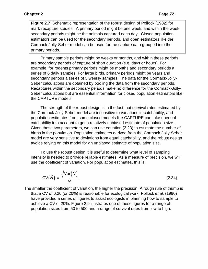
Chapter 2 Page 72
Figure 2.7 Schematic representation of the robust design of Pollock (1982) for
mark-recapture studies. A primary period might be one week, and within the week
secondary periods might be the animals captured each day. Closed population
estimators can be used for the secondary periods, and open estimators like the
Cormack-Jolly-Seber model can be used for the capture data grouped into the
primary periods.
Primary sample periods might be weeks or months, and within these periods
are secondary periods of capture of short duration (e.g. days or hours). For
example, for rodents primary periods might be months and secondary periods a
series of 6 daily samples. For large birds, primary periods might be years and
secondary periods a series of 5 weekly samples. The data for the Cormack-Jolly-
Seber calculations are obtained by pooling the data from the secondary periods.
Recaptures within the secondary periods make no difference for the Cormack-Jolly-
Seber calculations but are essential information for closed population estimators like
the CAPTURE models.
The strength of the robust design is in the fact that survival rates estimated by
the Cormack-Jolly-Seber model are insensitive to variations in catchability, and
population estimates from some closed models like CAPTURE can take unequal
catchability into account to get a relatively unbiased estimate of population size.
Given these two parameters, we can use equation (2.23) to estimate the number of
births in the population. Population estimates derived from the Cormack-Jolly-Seber
model are very sensitive to deviations from equal catchability, and the robust design
avoids relying on this model for an unbiased estimate of population size.
To use the robust design it is useful to determine what level of sampling
intensity is needed to provide reliable estimates. As a measure of precision, we will
use the coefficient of variation. For population estimates, this is:
( )( )ˆVar
ˆCVˆ
NN
N= (2.34)
The smaller the coefficient of variation, the higher the precision. A rough rule of thumb is
that a CV of 0.20 (or 20%) is reasonable for ecological work. Pollock et al. (1990)
have provided a series of figures to assist ecologists in planning how to sample to
achieve a CV of 20%. Figure 2.9 illustrates one of these figures for a range of
population sizes from 50 to 500 and a range of survival rates from low to high.

Chapter 2 Page 73
Figure 2.8 Relative precision of the Cormack-Jolly-Seber estimate of population
size for a range of population sizes from 50 to 500 when there are 10 sampling
periods and the survival rate Φ varies from 0.25 to 0.90 per primary interval. (From
Pollock et al. (1990).
Four general principles are illustrated in this graph:
1. Precision increases as the capture probability of individuals increases.
2. As the number of sampling times increases, precision increases.
3. If survival rates are higher, precision is also higher.
4. Precision increases as population size increases, for fixed survival rates,
number of samples, and capture probability.
For Cormack-Jolly-Seber estimates, the precision of estimating survival probabilities is
nearly the same as that of estimating population size, but it is more difficult to
estimate birth rates. Figure 2.9 illustrates this difference for one set of population
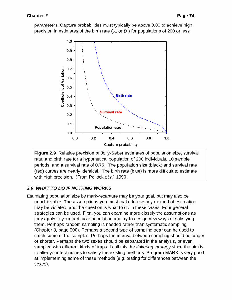
Chapter 2 Page 74
parameters. Capture probabilities must typically be above 0.80 to achieve high
precision in estimates of the birth rate (tort B ) for populations of 200 or less.
Figure 2.9 Relative precision of Jolly-Seber estimates of population size, survival
rate, and birth rate for a hypothetical population of 200 individuals, 10 sample
periods, and a survival rate of 0.75. The population size (black) and survival rate
(red) curves are nearly identical. The birth rate (blue) is more difficult to estimate
with high precision. (From Pollock et al. 1990.
2.6 WHAT TO DO IF NOTHING WORKS
Estimating population size by mark-recapture may be your goal, but may also be
unachievable. The assumptions you must make to use any method of estimation
may be violated, and the question is what to do in these cases. Four general
strategies can be used. First, you can examine more closely the assumptions as
they apply to your particular population and try to design new ways of satisfying
them. Perhaps random sampling is needed rather than systematic sampling
(Chapter 8, page 000). Perhaps a second type of sampling gear can be used to
catch some of the samples. Perhaps the interval between sampling should be longer
or shorter. Perhaps the two sexes should be separated in the analysis, or even
sampled with different kinds of traps. I call this the tinkering strategy since the aim is
to alter your techniques to satisfy the existing methods. Program MARK is very good
at implementing some of these methods (e.g. testing for differences between the
sexes).
Capture probability
0.0 0.2 0.4 0.6 0.8 1.0
Co
eff
icie
nt
of
Va
ria
tio
n
0.0
0.1
0.2
0.3
0.4
0.5
0.6
0.7
0.8
0.9
1.0
Birth rate
Population size
Survival rate
Chapter 2 Page 75
A second strategy is to use a very general, empirical model of population
estimation. Caughley (1977, p. 152) has reviewed this approach and emphasized its
value for practical work. The major assumption of these general models is that the
population is closed so there is no mortality during the marking experiment, and
consequently they are useful only for intensive short-term sampling. The basic data
of these models are the number of individuals caught once, twice, three times and
so on (frequency of capture approach). These data form a zero-truncated frequency
distribution of captures, and the missing zero- class represents the unknown number
of individuals that were never caught. A variety of statistical distributions can be
fitted to these data, and one stops once a "good fit" is achieved. Figure 2.10
illustrates this approach and Caughley (1977) provides details for the necessary
calculations, included in a Fortran computer program available in Program RECAP
(Appendix 2, page 000).
Chao (1988) provided another approach to data on frequency of capture data.
She used data from known populations enclosed in a fence to test the accuracy of
her approach. She presented two estimators, depending on whether the majority of
animals were caught 1-2 times or 1-3 times. The simplest Chao estimator is given
by:
( )2
1 2ˆ / 2N S f f = + (2.35)
where S is the number of individuals caught in the t samples
f1 is the number of animals caught only once
f2 is the number of animals caught twice
If there are sufficient numbers of individuals caught 3 times, the modified Chao
estimator is given by:
( ) ( ) ( ) ( ) 2
1 2 2 1 3 2/ 2 1 2 / / 1 3 /N S f f f t f f t f = + − − (2.36)
which uses the numbers of animals caught once, twice, and three times in the t
samples. These estimators can be calculated in Program CAUGHLEY (Appendix 2).
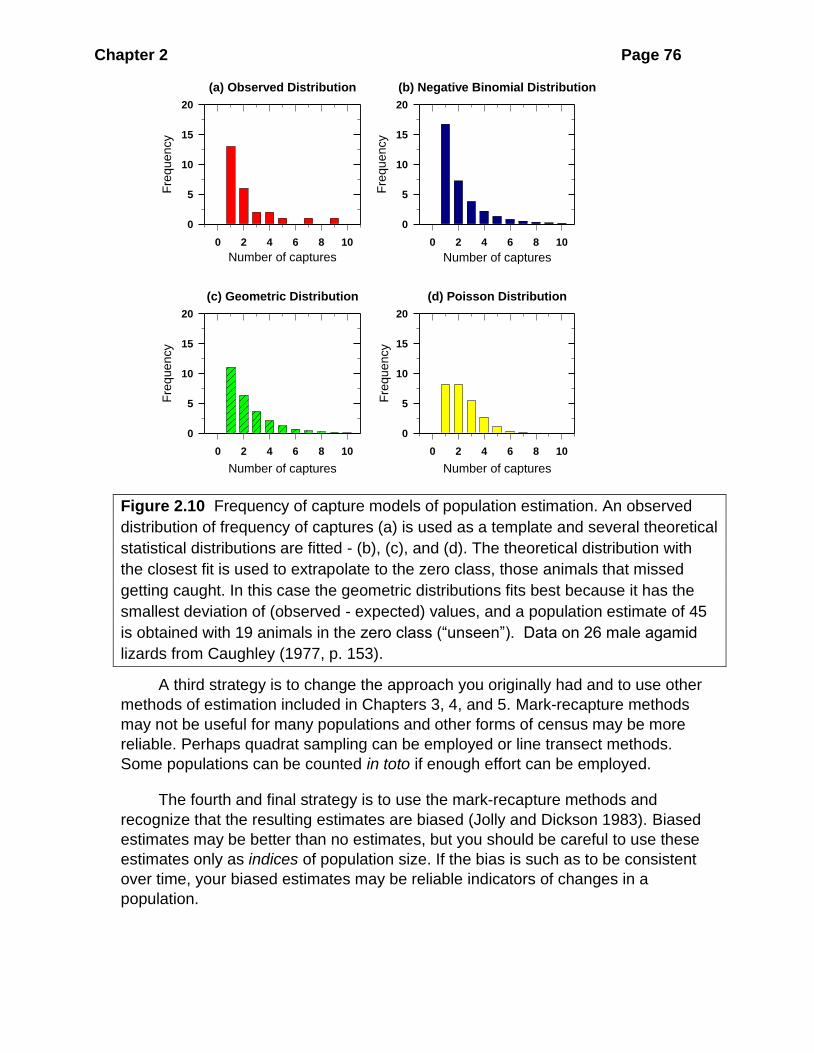
Chapter 2 Page 76
Figure 2.10 Frequency of capture models of population estimation. An observed
distribution of frequency of captures (a) is used as a template and several theoretical
statistical distributions are fitted - (b), (c), and (d). The theoretical distribution with
the closest fit is used to extrapolate to the zero class, those animals that missed
getting caught. In this case the geometric distributions fits best because it has the
smallest deviation of (observed - expected) values, and a population estimate of 45
is obtained with 19 animals in the zero class (“unseen”). Data on 26 male agamid
lizards from Caughley (1977, p. 153).
A third strategy is to change the approach you originally had and to use other
methods of estimation included in Chapters 3, 4, and 5. Mark-recapture methods
may not be useful for many populations and other forms of census may be more
reliable. Perhaps quadrat sampling can be employed or line transect methods.
Some populations can be counted in toto if enough effort can be employed.
The fourth and final strategy is to use the mark-recapture methods and
recognize that the resulting estimates are biased (Jolly and Dickson 1983). Biased
estimates may be better than no estimates, but you should be careful to use these
estimates only as indices of population size. If the bias is such as to be consistent
over time, your biased estimates may be reliable indicators of changes in a
population.
(a) Observed Distribution
Number of captures
0 2 4 6 8 10
Fre
qu
en
cy
0
5
10
15
20
(c) Geometric Distribution
Number of captures
0 2 4 6 8 10
Fre
qu
en
cy
0
5
10
15
20
(b) Negative Binomial Distribution
Number of captures
0 2 4 6 8 10
Fre
qu
en
cy
0
5
10
15
20
(d) Poisson Distribution
Number of captures
0 2 4 6 8 10
Fre
qu
en
cy
0
5
10
15
20

Chapter 2 Page 77
The principal recommendations of this chapter can be summarized as three
rules of procedure:
• Rule 1: Evaluate your objectives before starting, and do not assume that mark-
recapture methods are the easiest path to valid population estimates.
• Rule 2: Pick your mark-recapture method before starting field work, and build into
your sampling program a test of the model's assumptions.
• Rule 3: Treat all population estimates and confidence intervals with caution, and
recheck your assumptions as often as possible.
There is a considerable literature on more specialized techniques of mark-recapture
estimation. Seber (1982), Amstrup et al. (2006) and Cooch and White (2010) cover
all these problems in more detail.
2.7 SUMMARY
In both population and community ecology the single most important variable that must
be estimated is the size of a particular population or series of populations. One way
to do this is to use mark-recapture methods. Two general types are available,
depending on whether the population is closed or open.
Closed populations do not change in size during the sampling period, and thus
sampling must be done over a short time period. When only one period of marking
and recapture is available, the Petersen method is appropriate. When several
samples are taken with marking and recapturing, the Schnabel method or the
Schumacher-Eschmeyer method can be used. More advanced models are available
in Program CAPTURE and Program MARK if individuals are tagged and 3 or more
sampling sessions are carried out. The assumptions that are most critical are that
sampling is random and that marking animals does not affect their catchability. A
test of these assumptions is critical in any mark-recapture study.
Open populations change in size continuously, and the Cormack-Jolly-Seber
model is the best for analysis. The critical question for each marked individual
caught is: when was this individual last caught? Populations can be sampled over
many years with this approach, and in addition to population estimates, the
Cormack-Jolly-Seber model provides estimates of the probability of survival and the
recruitment (dilution) rate between the sampling times. For long term studies a
robust design is recommended in which both open and closed estimators can be
applied to the recapture data.
One critical assumption of all mark-recapture models is that animals are
equally catchable, so that marked individuals at any given sampling time have the
same chances of capture as unmarked individuals. This assumption is often violated
in natural populations, and statistical models in CAPTURE and MARK can test this
critical assumption in a variety of sampling situations with closed populations.

Chapter 2 Page 78
Mark-recapture techniques are difficult to use in the real world, and you should
be certain they are needed before starting to use these techniques. A guide to the
intensity of sampling required to attain reliable data is provided for open populations.
High capture probabilities are typically needed to obtain reliable data. For many
organisms there are easier ways of estimating abundance. The next three chapters
describe some alternative approaches.
SELECTED READING
Amstrup, S., MacDonald, L., and Manly, B. 2006. Handbook of Capture-Recapture
Analysis. Princeton University Press, Princeton, New Jersey. 296 pp.
Brown, L.D., Cai, T.T. & DasGupta, A. (2001) Interval estimation for a binomial
proportion. Statistical Science, 16(2): 101-117.
Conroy, M.J., Hines, J.E., Nichols, J.D., and Krementz, D.G. 2000. Simultaneous use of
mark-recapture and radiotelemetry to estimate survival, movement, and capture
rates. Journal of Wildlife Management 64(1): 302-313.
Karanth, K.U., and Nichols, J. 1998. Estimation of tiger densities in India using
photographic captures and recaptures. Ecology 79(8): 2852-2862.
Kendall, W.L. 1999. Robustness of closed capture-recapture methods to violations of
the closure assumption. Ecology 80(8): 2517-2525.
Lukacs, P.M., and Burnham, K.P. 2005. Estimating population size from DNA-based
closed capture-recapture data incorporating genotyping error. Journal of Wildlife
Management 69(1): 396-403.
Otis, D.L., Burnham, K.P., White, G.C. and Anderson, D.R. 1978. Statistical inference
from capture data on closed animal populations. Wildlife Monographs 62: 1-135.
Pollock, K.H., J.D. Nichols, C. Brownie, and J.E. Hines. 1990. Statistical inference for
capture-recapture experiments. Wildlife Monographs 107: 1-97.
Seber, G.A.F. 1982. The Estimation of Animal Abundance and Related Parameters. 2nd
edition. Griffin, London.
White, G.C. 2008. Closed population estimation models and their extensions in program
MARK. Environmental and Ecological Statistics 15(1): 89-99.
Williams, B.K., Nichols, J.D., and Conroy, M.J. 2002. Analysis and Management of
Animal Populations. Academic Press, New York.
QUESTIONS AND PROBLEMS
2.1. Villette (2010) marked red-backed voles with ear tags and recaptured them the
following morning by live trapping. She got these results for August 2009
number marked and released on day 1 = 48

Chapter 2 Page 79
number of caught on day 2 = 57
number caught on day 2 that were already marked = 40
She got these results for July 2010:
number marked and released on day 1 = 9
number of caught on day 2 = 9
number caught on day 2 that were already marked = 7
Calculate population estimates and their 95% confidence limits for these two data sets.
What assumptions must you make to calculate this estimate?
2.2. Wood (1963) sampled climbing cutworms at night, marked them with a fluorescent
powder, and resampled the population the next night. He obtained these data for
1962:
M = 1000 (first night)
C = 1755 second night
R = 41
Calculate the estimated population size and its 95% confidence interval for these data.
2.3. Hayne (1949) marked and released meadow voles in Michigan over five days with
the following results:
Date Total catch No. marked No. accidental deaths
July 19 p.m. 8 0 0
July 20 a.m. 19 0 0
July 20 p.m. 10 2 1
July 21 a.m. 23 8 0
July 21 p.m. 9 0 0
July 22 a.m. 14 9 0
July 22 p.m. 9 7 1
July 23 a.m. 21 13 0
Calculate an appropriate estimate of population size and justify your choice of
methods.
2.4. Dunnet (1963) sampled quokkas (small marsupials) on Rottnest Island off Western
Australia over three sampling periods with these results for 1957:
Mature animals Immature animals
Number marked at time 1 32 35
Number marked at time 1
and never seen again
22 20

Chapter 2 Page 80
Number marked caught at
times 1 and 2 only
5 1
Number marked caught at
times 1 and 3 only
4 11
Number marked caught at
times 1, 2 and 3
1 3
Number marked first at time
2 and never seen again
38 28
Number marked first at time
3
26 23
Number marked caught at
times 2 and 3 only
4 7
Recast these data in the form of an X-matrix, and use Program CAPTURE to estimate
the size of the mature population and the immature population of this marsupial.
What model is selected by Program CAPTURE, and how different are the
estimates from the different models available in this program? Do the tests in
Program CAPTURE suggest any evidence for unequal catchability in these data?
2.5. Leslie et al. (1953) tallied the following Method B table for a population of field voles
in Wales: No breeding occurred between October 1948 and April 1949. Estimate
the population parameters for these voles, and discuss the biological implications
of these estimates. Compare your analysis with that in Leslie et al. (1953, p. 144).
Time of Capture
Time of last
capture
Jun
e
July Sept. Oct
.
Nov
.
March April May Jun
e
July Sep
t
.
1948 June 12 7 4 0 1 1 0 0 0 0
July 10 0 1 0 0 0 0 0 0
Sept. 19 8 4 3 0 0 0 0
Oct. 11 9 1 2 0 0 0
Nov. 14 6 2 1 1 0
1949 March 46 11 4 0 0
April 34 18 0 0
May 34 3 1
June 40 5
July 56
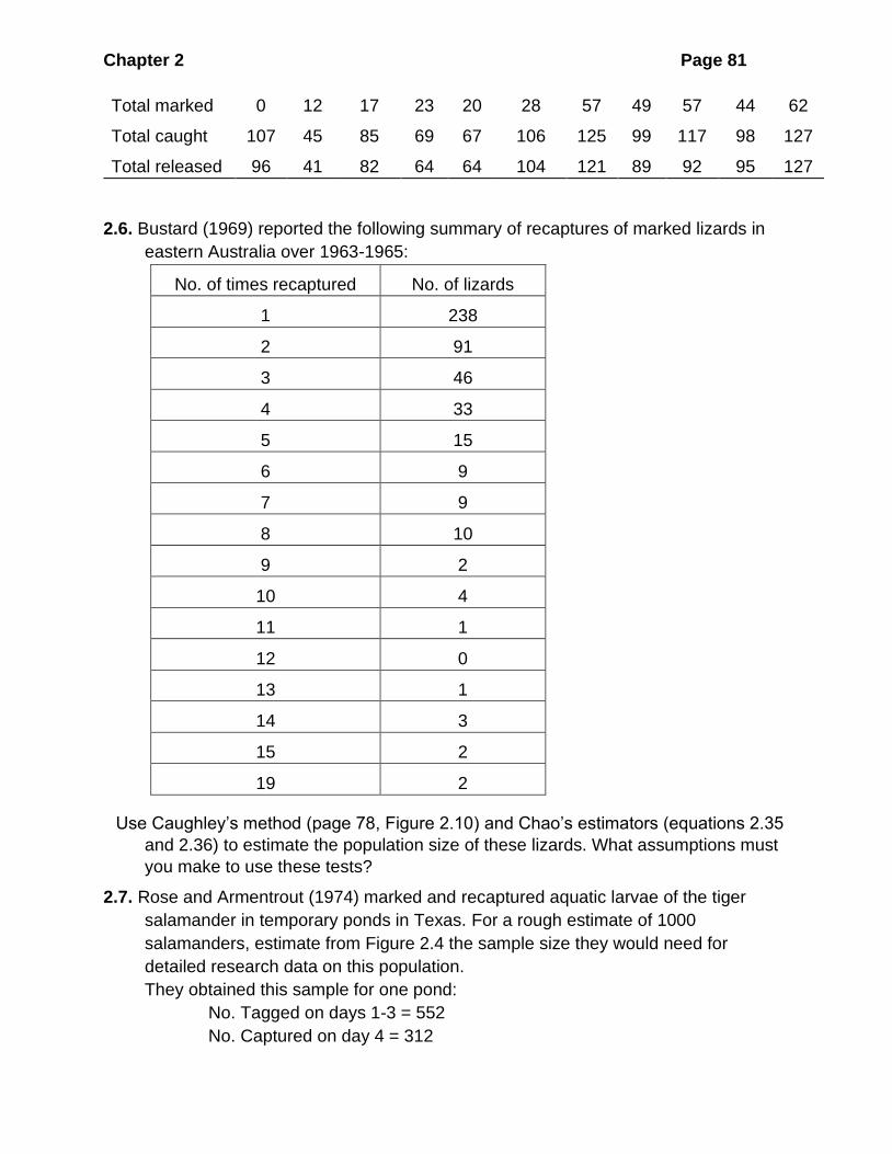
Chapter 2 Page 81
Total marked 0 12 17 23 20 28 57 49 57 44 62
Total caught 107 45 85 69 67 106 125 99 117 98 127
Total released 96 41 82 64 64 104 121 89 92 95 127
2.6. Bustard (1969) reported the following summary of recaptures of marked lizards in
eastern Australia over 1963-1965:
No. of times recaptured No. of lizards
1 238
2 91
3 46
4 33
5 15
6 9
7 9
8 10
9 2
10 4
11 1
12 0
13 1
14 3
15 2
19 2
Use Caughley’s method (page 78, Figure 2.10) and Chao’s estimators (equations 2.35
and 2.36) to estimate the population size of these lizards. What assumptions must
you make to use these tests?
2.7. Rose and Armentrout (1974) marked and recaptured aquatic larvae of the tiger
salamander in temporary ponds in Texas. For a rough estimate of 1000
salamanders, estimate from Figure 2.4 the sample size they would need for
detailed research data on this population.
They obtained this sample for one pond:
No. Tagged on days 1-3 = 552
No. Captured on day 4 = 312
Chapter 2 Page 82
No. Tagged Individuals on day 4 = 200
Calculate the population estimate for these data, and compare with the known
value of 875 salamanders for this pond. Was the estimated population size close
to the true value?
2.8. Carothers (1973) used mark recapture methods to estimate the number of taxi cabs
in Edinburgh, Scotland. He could determine that the known population was 420
cabs. In one of his samples over 5 days he obtained these data:
cabs counted only one time =135
cabs counted twice = 42
cabs counted three times = 9
cabs counted four times = 1
Estimate the size of this population and compare it with the known number of cabs.
2.9. Since all field populations of animals are open populations, why would you ever
use closed population estimators to determine population size?
2.10. Is it ever possible to have a Petersen population estimate that is lower than the
actual number of individuals caught? Can the lower confidence limits of a Petersen
estimate ever be below the actual number of individuals caught?
2.11. Chao (1988) reported capture data on the striped skunk as follows:
Capture frequency 1977 (8 trap
nights
1978 (4 trap
nights)
Caught once (f1) 2 10
Caught twice (f2) 7 4
Caught three times
(f3) 5 1
Caught four times
(f4) 3 2
Caught five times
(f5) 2
No. individuals
caught 19 17

Chapter 2 Page 83
Known population
size 23 28
Calculate the Schnabel and the Chao estimators for these two samples and discuss
which estimate is closer to the true value and why.