estimating aboveground tree biomass and leaf area index in ... · biomass and lai, the undergrowth...
TRANSCRIPT

Estimating aboveground tree biomass and leaf area index in a mountainbirch forest using ASTER satellite data
J. HEISKANEN
Department of Geography, University of Helsinki, P.O. Box 64, FIN-00014 University
of Helsinki, Finland
(Received 1 September 2005 )
Biomass and leaf area index (LAI) are important variables in many ecological
and environmental applications. In this study, the suitability of visible to
shortwave infrared advanced spaceborne thermal emission and reflection
radiometer (ASTER) data for estimating aboveground tree and LAI in the
treeline mountain birch forests was tested in northernmost Finland. The biomass
and LAI of the 128 plots were surveyed, and the empirical relationships between
forest variables and ASTER data were studied using correlation analysis and
linear and non-linear regression analysis. The studied spectral features also
included several spectral vegetation indices (SVI) and canonical correlation
analysis (CCA) transformed reflectances. The results indicate significant
relationships between the biomass, LAI and ASTER data. The variables were
predicted most accurately by CCA transformed reflectances, the approach
corresponding to the multiple regression analysis. The lowest RMSEs were
3.45 t ha21 (41.0%) and 0.28 m2m22 (37.0%) for biomass and LAI respectively.
The red band was the band with the strongest correlation against the biomass
and LAI. SR and NDVI were the SVIs with the strongest linear and non-linear
relationships. Although the best models explained about 85% of the variation in
biomass and LAI, the undergrowth vegetation and background reflectance are
likely to affect the observed relationships.
1. Introduction
The birch forests cover considerable areas north of the boreal coniferous forest belt
in northern Fennoscandia (Hamet-Ahti 1963, Wielgolaski 1997). Mountain birch
(Betula pubescens ssp. czerepanovii) is the most common tree or scrub in the area
forming the treeline both to the north and at high elevations. The mountain birch
forests are subject to natural and human induced changes, which emphasise the needfor monitoring the dynamics of these ecosystems. The forests are affected by the
grazing and trampling of semi-domestic reindeer (Helle 2001) and defoliated
regularly over vast areas by insect herbivores (Neuvonen et al. 2001). Mountain
birch ecosystems are also likely to be affected by climate change (Skre 2001).
Observations from the Swedish Scandes indicate that the birch treeline is already
slowly advancing (Kullman 2000).
Biomass and leaf area index (LAI) are important variables in many ecological and
environmental applications, for example, in the regional ecosystem models (Nemani
et al. 1993, Waring and Running 1998). Accurate estimation of biomass is required
*Email: [email protected]
International Journal of Remote Sensing
Vol. 27, No. 6, 20 March 2006, 1135–1158
International Journal of Remote SensingISSN 0143-1161 print/ISSN 1366-5901 online # 2006 Taylor & Francis
http://www.tandf.co.uk/journalsDOI: 10.1080/01431160500353858
for carbon stock accounting and monitoring (Brown 2002, Rosenqvist et al. 2003).
LAI is defined as one half of the total leaf area per unit ground surface area (Chen
and Black 1991), and it controls many biological and physical processes in the water,
nutrient and carbon cycle (Waring and Running 1998).
However, there are only a few studies concerning the biomass and LAI of the
mountain birch forests. Starr et al. (1998), Bylund and Nordell (2001) and Dahlberg
et al. (2004) have studied the biomass proportioning of mountain birch trees, and
developed allometric relationships to approximate the biomass of a tree component
or the total biomass of single trees according to some more easily measured variable,
such as diameter at breast height or height. The allometric relationships have been
applied to estimate the biomass for the sample plots (Starr et al. 1998, Bylund and
Nordell 2001). Furthermore, Dahlberg et al. (2004) presented vegetation type
averaged biomass and LAI estimates. However, in addition to these studies there is
also a need for regional biomass and LAI estimates.
The possibility of estimating biomass and LAI by satellite remote sensing has
been investigated in several studies at various spatial scales and environments
(Badhwar et al. 1986, Spanner et al. 1990, Nemani et al. 1993, Chen and Cihlar 1996,
Fassnacht et al. 1997, Hame et al. 1997, Myneni et al. 1997, Turner et al. 1999,
Brown et al. 2000, Brown 2001, Chen et al. 2002, Tomppo et al. 2002, Eklundh et al.
2003, Laidler and Treitz 2003, Stenberg et al. 2004). The most frequently used
remote sensing data continue to be from the optical moderate resolution sensors,
like Landsat Enhanced Thematic Mapper Plus (ETM + ). However, few remote
sensing studies have attempted to estimate biomass and LAI for mountain birch
forests (Dahlberg 2001), although the studies from the boreal coniferous forests and
arctic tundra are abundant. Most of the remote sensing studies concerning the
mountain birch forests have concentrated on image classification (Kayhko and
Pellikka 1994, Colpaert et al. 2003).
Typically, the estimation of the forest variables using optical remote sensing data
has been based on empirical relationships formulated between the forest variables
measured in the field and satellite data, often expressed in the form of spectral
vegetation indices (SVI) (table 1). In general, SVIs attempt to enhance the spectral
contribution of vegetation while minimising that of the background. SVIs using
some combination of red and near-infrared (NIR) reflectances, like the simple
ratio (SR) and the normalised difference vegetation index (NDVI) have been
particularly popular. However, the empirical relationships are affected by various
factors, including canopy closure, understory vegetation and background reflec-
tance (Spanner et al. 1990). A set of soil-adjusted vegetation indices have been
developed to reduce the effects of the soil background reflectance (Huete 1988,
Major et al. 1990, Qi et al. 1994, Rondeaux et al. 1996). Furthermore, some
studies have stated that the inclusion of the shortwave infrared (SWIR) into the
SVIs would unify different cover types and reduce the background effects (Nemani
et al. 1993, Brown et al. 2000). It is obvious that the effect of the background
reflectance is pronounced in the treeline, where canopy closure varies considerably
(Brown 2001).
If we wish to use satellite data to map the biomass and LAI of the mountain birch
forests, it is necessary to understand how these variables relate to the satellite
observed reflectance. The aim of this study was to examine the potential of the
visible to shortwave infrared advanced spaceborne thermal emission and reflection
radiometer (ASTER) satellite data for estimating biomass and LAI in the mountain
1136 J. Heiskanen
birch forest in northernmost Finland. The statistical relationships between the
field measured biomass, LAI and ASTER satellite data were studied using
correlation analysis, and models developed by linear and non-linear regression
analyses. The studied spectral features included the single spectral bands,
several common SVIs, and canonical correlation analysis (CCA) transformed
reflectances.
ASTER data was employed because it has relatively high spatial resolution in the
visible to near infrared bands, and high spectral resolution in the shortwave infrared
bands (Yamaguchi et al. 1998). The provision of higher order data products, such as
atmospherically corrected surface reflectance data, is also increasing the applica-
bility of ASTER data (Abrams 2000). Furthermore, ASTER has been used only
very little in the study of forests.
2. Materials and methods
2.1 Study area
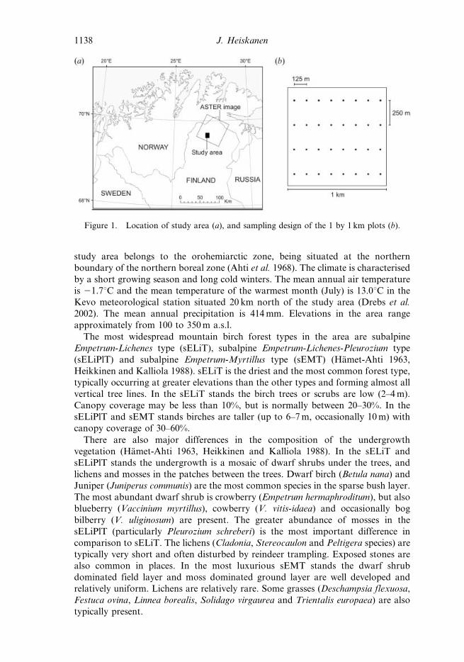
The study area is located in the Utsjoki region, in northernmost Finland (figure 1a).
The area lies north of the continuous pine forest and is characterised by subalpine
mountain birch forests, gently sloping low fells and mires. In terms of vegetation the
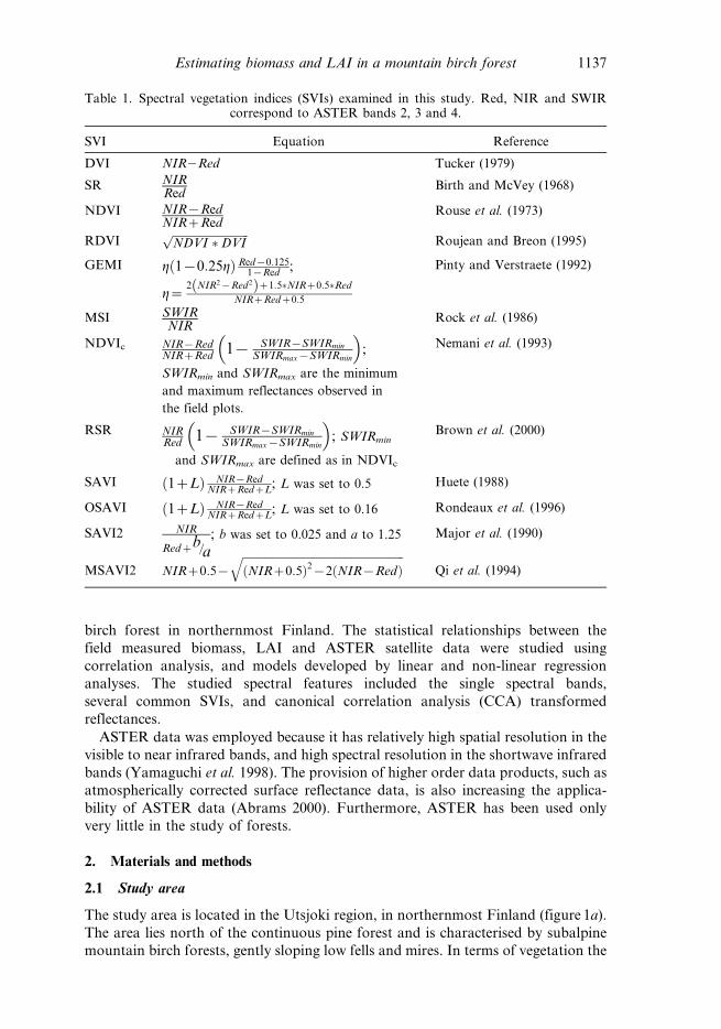
Table 1. Spectral vegetation indices (SVIs) examined in this study. Red, NIR and SWIRcorrespond to ASTER bands 2, 3 and 4.
SVI Equation Reference
DVI NIR2Red Tucker (1979)
SR NIRRed
Birth and McVey (1968)
NDVI NIR{RedNIRzRed
Rouse et al. (1973)
RDVIffiffiffiffiffiffiffiffiffiffiffiffiffiffiffiffiffiffiffiffiffiffiffiffiffiffiffiffi
NDVI �DVIp
Roujean and Breon (1995)
GEMI g 1{0:25gð Þ Red{0:1251{Red
;
g~2 NIR2{Red2ð Þz1:5�NIRz0:5�Red
NIRzRedz0:5
Pinty and Verstraete (1992)
MSI SWIRNIR
Rock et al. (1986)
NDVIc NIR{RedNIRzRed
1{ SWIR{SWIRmin
SWIRmax{SWIRmin
� �
;
SWIRmin and SWIRmax are the minimum
and maximum reflectances observed in
the field plots.
Nemani et al. (1993)
RSR NIRRed
1{ SWIR{SWIRmin
SWIRmax{SWIRmin
� �
; SWIRmin
and SWIRmax are defined as in NDVIc
Brown et al. (2000)
SAVI 1zLð Þ NIR{RedNIRzRedzL
; L was set to 0.5 Huete (1988)
OSAVI 1zLð Þ NIR{RedNIRzRedzL
; L was set to 0.16 Rondeaux et al. (1996)
SAVI2 NIR
Redzb=a; b was set to 0.025 and a to 1.25 Major et al. (1990)
MSAVI2 NIRz0:5{
ffiffiffiffiffiffiffiffiffiffiffiffiffiffiffiffiffiffiffiffiffiffiffiffiffiffiffiffiffiffiffiffiffiffiffiffiffiffiffiffiffiffiffiffiffiffiffiffiffiffiffiffiffiffiffiffiffiffiffi
NIRz0:5ð Þ2{2 NIR{Redð Þq
Qi et al. (1994)
Estimating biomass and LAI in a mountain birch forest 1137
study area belongs to the orohemiarctic zone, being situated at the northern
boundary of the northern boreal zone (Ahti et al. 1968). The climate is characterised
by a short growing season and long cold winters. The mean annual air temperature
is 21.7uC and the mean temperature of the warmest month (July) is 13.0uC in the
Kevo meteorological station situated 20 km north of the study area (Drebs et al.
2002). The mean annual precipitation is 414 mm. Elevations in the area range
approximately from 100 to 350 m a.s.l.
The most widespread mountain birch forest types in the area are subalpine
Empetrum-Lichenes type (sELiT), subalpine Empetrum-Lichenes-Pleurozium type
(sELiPlT) and subalpine Empetrum-Myrtillus type (sEMT) (Hamet-Ahti 1963,
Heikkinen and Kalliola 1988). sELiT is the driest and the most common forest type,
typically occurring at greater elevations than the other types and forming almost all
vertical tree lines. In the sELiT stands the birch trees or scrubs are low (2–4 m).
Canopy coverage may be less than 10%, but is normally between 20–30%. In the
sELiPlT and sEMT stands birches are taller (up to 6–7 m, occasionally 10 m) with
canopy coverage of 30–60%.
There are also major differences in the composition of the undergrowth
vegetation (Hamet-Ahti 1963, Heikkinen and Kalliola 1988). In the sELiT and
sELiPlT stands the undergrowth is a mosaic of dwarf shrubs under the trees, and
lichens and mosses in the patches between the trees. Dwarf birch (Betula nana) and
Juniper (Juniperus communis) are the most common species in the sparse bush layer.
The most abundant dwarf shrub is crowberry (Empetrum hermaphroditum), but also
blueberry (Vaccinium myrtillus), cowberry (V. vitis-idaea) and occasionally bog
bilberry (V. uliginosum) are present. The greater abundance of mosses in the
sELiPlT (particularly Pleurozium schreberi) is the most important difference in
comparison to sELiT. The lichens (Cladonia, Stereocaulon and Peltigera species) are
typically very short and often disturbed by reindeer trampling. Exposed stones are
also common in places. In the most luxurious sEMT stands the dwarf shrub
dominated field layer and moss dominated ground layer are well developed and
relatively uniform. Lichens are relatively rare. Some grasses (Deschampsia flexuosa,
Festuca ovina, Linnea borealis, Solidago virgaurea and Trientalis europaea) are also
typically present.
Figure 1. Location of study area (a), and sampling design of the 1 by 1 km plots (b).
1138 J. Heiskanen

2.2 Field data
The field data were surveyed in July 2004. The data were collected from four
1*1 km2 study sites located in the different mountain birch forest types with variable
tree and shrub covers. The study sites were chosen using the biotope inventory map
and database over northernmost Finland (Sihvo 2001). The sampling design of the
study sites is shown in figure 1b. Each site was surveyed by four transects located
250 m apart from each other, consisting of eight plots 125 m apart from each other.
The plot size was 100 m2 in the densest site and 200 m2 in the three sparser sites. The
centre points of the plots were located using a handheld GPS device (Magellan
Meridian Platinum). According to the manufacturer the device should have an
accuracy of 7 m for 95% of time. Furthermore, the GPS measurements were
averaged over several minutes in order to enhance the accuracy.
The surveyed data consisted of the basic stand parameters for scrubs and trees
taller than 1.3 m. Diameter at breast height (1.3 m) was measured for every tree, and
height for every tenth tree. The canopy closure of the densest plots was estimated
from hemispherical photographs (e.g. Rich 1990). The vegetation type and the
undergrowth composition were also recorded.
The biomass of stem, live branches, dead branches and leaves were estimated
using the diameter at breast height measurements and the allometric models
developed for mountain birch by Starr et al. (1998). The biomass proportions were
summed to give the aboveground tree biomass (hence called biomass). These values
were converted into biomass in t ha21 using the area of the plot. The leaf area was
estimated using the estimated leaf biomass and specific leaf weight (79.48 g m22)
measured by Kause et al. (1999). The estimated leaf area was converted into LAI
(m2 m22) using the area of the plot.
Altogether 128 plots were measured in the study area, 45 plots belonging to the
sELiT type, 56 to the sELiPlT type and 23 plots to the sEMT type. Four plots were
excluded since plots were not located on mineral soils. Table 2 shows the descriptive
statistics for the field data. The canopy closure of the densest plots was estimated to
be around 50–60% (max563%).
2.3 Remotely sensed data
A cloudless ASTER scene (AST_L1B.003: 2014007270) recorded on 29 July 2000
and processed into a level 2 surface reflectance (AST_07) product (Abrams 2000)
was used in this study. The coverage of the image is shown in figure 1a.
Table 2. Descriptive statistics of the field data (n5124).
Variable Mean SD Min Max
Tree density (trees ha21) 2709 1792 0.00 9205Basal area (m2 ha21) 3.11 3.08 0.00 12.38Mean height (m) 2.85 0.74 0.00 4.96Total tree biomass (t ha21) 8.35 8.31 0.00 33.26Stem biomass (t ha21) 5.18 5.27 0.00 21.24Live branch biomass (t ha21) 2.41 2.36 0.00 9.51Dead branch biomass (t ha21) 0.16 0.16 0.00 0.65Leaf biomass (t ha21) 0.60 0.52 0.00 2.12LAI (m2 m22) 0.76 0.66 0.00 2.70
SD, standard deviation.
Estimating biomass and LAI in a mountain birch forest 1139
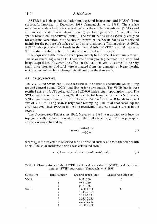
ASTER is a high spatial resolution multispectral imager onboard NASA’s Terra
spacecraft, launched in December 1999 (Yamaguchi et al. 1998). The surface
reflectance product has three spectral bands in the visible near-infrared (VNIR) and
six bands in the shortwave infrared (SWIR) spectral regions with 15 and 30 metres
spatial resolution, respectively (table 3). The VNIR bands were especially designed
for assessing vegetation, but the spectral ranges of the SWIR bands were selected
mainly for the purpose of surface soil and mineral mapping (Yamaguchi et al. 1998).
ASTER also provides five bands in the thermal infrared (TIR) spectral region at90 m spatial resolution, but this data were not used in this study.
The acquisition date corresponds approximately to the time of maximum leaf size.
The solar zenith angle was 51u. There was a four-year lag between field work and
image acquisition. However, the effect on the data analysis is assumed to be very
small since biomass and LAI were estimated from the diameter at breast height,
which is unlikely to have changed significantly in the four years.
2.4 Image processing
The VNIR and SWIR bands were rectified to the national coordinate system using
ground control points (GCPs) and first order polynomials. The VNIR bands wererectified using 41 GCPs collected from 1 : 20 000 scale digital topographic maps. The
SWIR bands were rectified using 28 GCPs collected from the rectified VNIR bands.
VNIR bands were resampled to a pixel size of 15*15 m2 and SWIR bands to a pixel
size of 30*30 m2 using nearest-neighbour resampling. The total root mean square
error was 0.65 pixels (9.75 m) in the first rectification and 0.58 pixels (17.4 m) in the
second.
The C-correction (Teillet et al. 1982, Meyer et al. 1993) was applied to reduce thetopographically induced variations in the reflectance (rT). The topographic
correction was achieved by:
rH~rT
cos hsð Þzc
cos ið Þzcð1Þ
where rH is the reflectance observed for a horizontal surface and hs is the solar zenith
angle. The solar incidence angle i was calculated from:
cos ið Þ~coshscoshnzsinhssinhncos ws{wnð Þ ð2Þ
Table 3. Characteristics of the ASTER visible and near-infrared (VNIR), and shortwaveinfrared (SWIR) subsystems (Yamaguchi et al. 1998).
Subsystem Band number Spectral range (mm) Spatial resolution (m)
VNIR 1 0.52–0.60 152 0.63–0.693 0.76–0.86
SWIR 4 1.600–1.700 305 2.145–2.1856 2.185–2.2257 2.235–2.2858 2.295–2.3659 2.360–2.430
1140 J. Heiskanen

where hn is the slope of the terrain surface, ws is the solar azimuth angle and wn is the
aspect of the slope. The slope and aspect were calculated from the DEM in
25*25 m2 pixel size. The cos(i) was resampled to match the pixel sise of the VNIR
and SWIR bands. The parameter c was determined by the linear regression analysis
(rT5a cos(i) + b, c5b/a). A forest mask was derived from the biotope inventory map
and slope mask (hn>5 degrees) from the DEM to limit the regression analysis to the
forested and inclined pixels.
The topographic correction reduced the correlation between the solar incidence
angle and surface reflectance very close to zero (table 4). This indicates that the
dependence between the variables was successfully removed.
2.5 Spectral feature extraction
Plotwise reflectances were derived from the image to examine the relationship
between biomass, LAI, and ASTER data. An average of reflectance inside 25 m
buffer zones was calculated, and the pixel was included to the buffer zone if its
midpoint was inside the border. The reflectances were determined for field plots
using on average nine VNIR pixels and two SWIR pixels. The averaging was
assumed to reduce the geometric errors both in the GPS measurements and in the
image rectification, and furthermore, remove the difference in the pixel size between
the VNIR and SWIR bands.
The reflectances were employed to calculate several frequently used SVIs (table 1).
ASTER band 2 was used as a red band, band 3 as a near-infrared band and band 4
as a shortwave-infrared band in the equations. The parameters of the soil line were
determined from the scatterplot of the red and near-infrared ASTER reflectances
(figure 2) to calculate SAVI2 (Major et al. 1990). The soil line was fitted to the
reflectance of the nonvegetated sandbars and stony areas. The darkest pixels
correspond to the water.
2.6 Data analysis
Two-thirds of the data (83 cases) were allocated by random sampling to the
modelling set and one-third (41 cases) to the validation set. The modelling set was
employed to examine the linear and non-linear relationships between forest
Table 4. Values of the parameter c employed in the topographic correction of the ASTERdata, and correlation (r) between the cosine of the solar incidence angle and reflectance before
and after the correction.
Band c
r
Before After
1 2.028 0.275 0.0192 0.751 0.200 0.0273 0.614 0.484 0.0244 0.579 0.551 0.0645 1.169 0.300 0.0206 0.772 0.341 0.0387 0.882 0.325 0.0358 0.839 0.291 0.0319 1.394 0.265 0.023
Estimating biomass and LAI in a mountain birch forest 1141

variables and spectral features using correlation analysis, and linear and non-linear
regression analysis. The estimation errors were studied by the validation set.
Curran and Hay (1986) and Cohen et al. (2003) have stated that the ordinary least
squares (OLS) regression is often an inappropriate method for relating remotely
sensed data to ground variables. The problem is that OLS assumes that it is possible
to specify ‘independent’ and ‘dependent’ variables, and that the independent
variable is measured without error. It is difficult to make the specification and fulfil
the assumptions in the case of remotely sensed data (Curran and Hay 1986).
Furthermore, the predictions by the OLS tend to have attenuated variation in the
direction of estimation compared to the observed values (Cohen et al. 2003). The
reduced major axis (RMA) regression was used in this study as recommended by
Curran and Hay (1986) and Cohen et al. (2003). The terms of the linear model
(y5ax + b) were calculated from (Curran and Hay 1986):
a~sy
sx
b~y{ax ð3Þ
where y and x are the means of the variables y and x, and sy and sx standard
deviations, respectively. The sign of the slope term a was determined from the
correlation analysis. The forest variables were y and spectral features x in the
analysis.
Multiple regression analysis using several spectral features is an alternative to the
simple linear regression. Canonical correlation analysis (CCA) enables multiple
regression analysis in a simple linear context (Cohen et al. 2003). CCA is a
multivariate statistical procedure that allows the interrelationships between two sets
of variables, in this case forest variable(s) and multispectral bands, to be
investigated. CCA maximises the correlation between sets of variables and provides
Figure 2. Scatterplot of the ASTER band 2 (red) and band 3 (near-infrared) reflectances,and the estimated soil line.
1142 J. Heiskanen
a set of weights for the spectral bands that aligns them with the variation in the
forest variable(s). The canonical weighs can be applied to the spectral bands to give
CCA scores corresponding to a single integrated index. The benefit over the multiple
linear regression analysis is that the single index facilitates the visual assessment of
model strength and linearity of the relationship, and enables the visualisation and
interpretation on screen equally to traditional vegetation indices. Furthermore,
CCA enables the use of RMA regression (Cohen et al. 2003).
In this study, the canonical weights were computed separately for biomass and
LAI, and reflectance values were converted to the corresponding CCA scores.
However, if all the spectral bands are involved in the CCA, some of the canonical
weights are very small due to redundancy effects. Redundancy was minimised by
selecting only the most significant variables using stepwise regression analysis before
the CCA. The criterion to eliminate and include variables was that all variables in
the models should be significant (p,0.05). CCA scores were used in the regression
analysis like all the other spectral features.
Several studies (e.g. Myneni et al. 1997) have reported non-linear relationships
between the forest variables and reflectance data. Therefore, also the log-
transformations of the ASTER bands, and the applicability of power law (y5axb)
and exponential (y5aebx) models were examined. The models were linearised and
parameters a and b estimated using RMA regression. The best type of model in
terms of coefficient of determination (R2) was chosen for each feature.
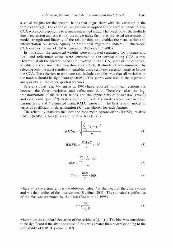
The reliability statistics included the root mean square error (RMSE), relative
RMSE (RMSEr), bias (Bias) and relative bias (Biasr):
RMSE~
ffiffiffiffiffiffiffiffiffiffiffiffiffiffiffiffiffiffiffiffiffiffiffiffiffiffi
P
n
i~1
yi{yið Þ2
n
v
u
u
u
t
ð4Þ
RMSEr~RMSE
y� 100 ð5Þ
Bias~
P
n
i~1
yi{yið Þ
nð6Þ
Biasr~Bias
y1100 ð7Þ
where yi is the estimate, yi is the observed value, y is the mean of the observations
and n is the number of the observations (Hyvonen 2002). The statistical significance
of the bias was estimated by the t-test (Ranta et al. 1998):
t~Bias
sD= ffiffiffi
np ð8Þ
where sD is the standard deviation of the residuals ( yi{yi). The bias was considered
to be significant if the absolute value of the t was greater than t corresponding to the
probability of 0.05 (Hyvonen 2002).
Estimating biomass and LAI in a mountain birch forest 1143

3. Results
3.1 Correlation between biomass, LAI and ASTER bands
All the spectral bands were significantly correlated (p,0.05) with biomass and LAI
(table 5). The correlation patterns were similar for both biomass and LAI due to a
strong positive correlation between these two parameters (r50.985). However, the
correlations were somewhat stronger with LAI than with biomass. Band 2,
corresponding to the red reflectance, was the band showing the strongest correlation
with biomass (r520.831) and LAI (r520.847). Also bands 3 and 4, corresponding
to the NIR and SWIR reflectance, were strongly correlated with biomass and LAI.
The correlation with band 3 was positive but otherwise the correlations were
negative. The standard logarithmic transformation of the reflectances enhanced the
correlation in all bands except in band 3. The band 2 had the strongest correlation
against biomass (20.872) and LAI (20.883) also after the transformation.
LAI is plotted against the reflectance in bands 2, 3 and 4 in figures 3(a)–3(c). The
scatterplots of the spectral bands versus biomass were very similar to those shown in
figures 3(a)–3(c), and hence are not shown here. The relationship between the band 2
Table 5. Correlations of the biomass and LAI against the ASTER reflectance, log-transformed ASTER reflectance, SVIs and CCA scores (n583). All the correlations are
significant (p,0.05).
Band or index Biomass LAI
Band 1 20.698 20.719Band 2 20.831 20.847Band 3 0.812 0.827Band 4 20.821 20.830Band 5 20.781 20.798Band 6 20.780 20.795Band 7 20.742 20.760Band 8 20.730 20.748Band 9 20.753 20.771Log (band 1) 20.721 20.741Log (band 2) 20.872 20.883Log (band 3) 0.792 0.810Log (band 4) 20.827 20.834Log (band 5) 20.805 20.819Log (band 6) 20.808 20.819Log (band 7) 20.777 20.792Log (band 8) 20.775 20.789Log (band 9) 20.783 20.798DVI 0.834 0.850SR 0.902 0.907NDVI 0.817 0.835RDVI 0.831 0.848GEMI 0.812 0.828MSI 20.805 20.823NDVIc 0.851 0.858RSR 0.884 0.882SAVI 0.832 0.849OSAVI 0.828 0.845SAVI2 0.888 0.897MSAVI2 0.846 0.861CCA scores 0.916 0.922
1144 J. Heiskanen

and LAI is curvilinear (figure 3(a)). The reduction in the reflectance is more rapid as
LAI increases in the sparsest sELiT type compared to the denser sELiPlT and sEMT
types. The relationship between band 3 and LAI is also curvilinear, because some of
the sparsest sELiT sites have very low reflectance in the NIR band (figure 3(b)).
Band 3 also has more scattering in the LAI values over 1 than band 2. The plots
belonging to the sEMT type seem to have relatively high reflectance in band 3compared to the other forest types. In contrast to bands 2 and 3, the relationship
between band 4 and LAI is relatively linear, but reflectance in band 4 is not as
sensitive to changes in LAI as reflectance in bands 2 and 3 (figure 3c). In general, all
the three bands begin to saturate at LAI values of approximately 2.
Figures 3(a)–3(c) also show the forest type specific correlations for bands 2, 3 and
4, and LAI. Generally speaking, the forest type specific correlations are lower than
correlations for pooled data. Band 2 is strongly correlated with LAI in all the forest
types. Bands 3 and 4 show weaker correlations, particularly in the densest sEMTtype. The relatively weak correlations in the sEMT type are also an indication of
weak sensitivity of the bands in the high values of LAI.
3.2 Correlation between biomass, LAI and SVIs
All of the SVIs were also significantly correlated (p,0.05) with biomass and LAI,
SR being the SVI showing the strongest correlations, 0.902 and 0.907, respectively
Figure 3. Relationship between LAI and ASTER band 2 (a), band 3 (b) and band 4 (c)reflectances, and relationship between LAI and SR (d). Correlation coefficients (r) are givenseparately for different mountain birch forest types and pooled data.
Estimating biomass and LAI in a mountain birch forest 1145

(table 5). Also SAVI2 and RSR were strongly correlated with the forest variables. In
comparison to the single bands, only SR and SAVI2 showed stronger correlations
with biomass and LAI than the log-transformed band 2.
The LAI is plotted against SR in figure 3(d). SR shows a strong linear relation
with LAI. The LAI has a stronger correlation with SR than with single bands 2 and
3, which were utilised in the calculation of SR. In the sEMT forest type the
correlation is weaker with SR than with band 2 due to a very low correlation with
band 3.
3.3 Canonical correlation analysis
Canonical correlation analysis was applied to convert the spectral bands into single
optimised indices. According to the stepwise multiple regression analysis the bands
1, 2, 3 and 9 were employed in the CCA. Bands 1, 2 and 9 were log-transformed
before the analysis, because the transformation enhanced the linear correlation. The
equations to calculate the CCA scores are given in the table 6.
The CCA scores showed a stronger correlation with biomass and LAI than with
single bands or SVIs, 0.916 and 0.922 respectively (table 3). The biomass and LAI
are plotted against CCA scores in figure 4. The relationships are relatively linear, but
the CCA scores are also insensitive to the variability in the highest biomass and LAI
values. Both the pooled and forest type specific correlations are also higher than
with any other feature.
Table 6. Equations to calculate CCA scores for biomass and LAI (n583).
Variable Equation
Biomass 7.938 Log (band 1)213.286 Log (band 2) + 9.309 Band 3 + 9.953 Log (band 9)LAI 6.255 Log (band 1)212.556 Log (band 2) + 10.914 Band 3 + 10.273 Log (band 9)
Figure 4. Relationship between biomass (a), LAI (b) and canonical correlation analysis(CCA) transformed reflectances (CCA scores). Correlation coefficients (r) are givenseparately for different mountain birch forest types and pooled data. The figure also showsthe linear model fitted by the regression analysis.
1146 J. Heiskanen

3.4 Models for biomass and LAI
The linear regression models for biomass and LAI, and the coefficients of
determination (R2), are shown in table 7. The R2 values of the linear models varied
between 0.63 and 0.84 for biomass, and between 0.63 and 0.85 for LAI. The highest
R2 values resulted by using the CCA scores, as expected. The models for biomass
and LAI using the CCA scores are shown in figure 4. The next best linear predictors
of the biomass were SR (R250.81), SAVI2 (0.79), RSR (0.78) and log (band 2)
(0.76). For LAI the R2 values were 0.82, 0.80, 0.78 and 0.78, respectively.
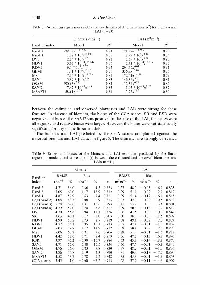
The non-linear regression models and R2 values are given in table 8. In the case of
band 4, SR, NDVIc and RSR the non-linear models could not enhance the R2 values
significantly and models were not developed. However, in the case of other bands
and SVIs the R2 values were improved considerably by the non-linear models.
NDVI had the highest R2 values for both the biomass (0.85) and LAI (0.83).
However, the differences to the next best models using band 2, OSAVI and SAVI
were very small. The power law type models were the most common, but the
exponential models produced the highest R2 values. In contrast to the linear models,
the R2 values were slightly better for biomass than for LAI.
3.5 Error statistics
The error statistics of the linear regression models are given in table 9. The table also
shows the correlation coefficients (r) between the estimated and observed biomasses
and LAIs. The lowest RMSE was 3.45 t ha21 (41.0%) for biomass and 0.28 m2m22
(37.0%) for LAI predicted by CCA scores. The next best predictors were SR, SAVI2,
RSR and log (band 2) with RMSEs between 3.63–4.08 t ha21 (43.1–48.5%) for
biomass, and between 0.30–0.33 m2m22 (38.7–43.6%) for LAI. Also, the correlations
Table 7. Linear regression models and coefficients of determination (R2) for biomass andLAI (n583).
Band or index
Biomass (t ha21) LAI (m2 m22)
Model R2 Model R2
Band 2 2652.36x + 35.79 0.69 250.44x + 2.86 0.72Band 3 284.10x258.33 0.66 21.97x24.42 0.68Band 4 2499.04x + 113.58 0.67 238.59x + 8.87 0.69Log (band 2) 262.32x278.73 0.76 24.82x26.00 0.78Log (band 3) 152.03x + 104.59 0.63 11.76x + 8.18 0.66Log (band 4) 2239.44x2153.85 0.68 218.51x211.81 0.70DVI 201.94x230.56 0.70 15.62x22.27 0.72SR 3.14x211.65 0.81 0.24x20.81 0.82NDVI 75.74x243.90 0.67 5.86x23.31 0.70RDVI 123.20x236.54 0.69 9.53x22.74 0.72GEMI 165.68x2-98.68 0.66 12.81x27.54 0.69MSI 245.65x + 50.40 0.65 23.53x + 3.99 0.68NDVIc 36.91x24.44 0.72 2.85x20.25 0.74RSR 2.68x21.34 0.78 0.21x20.01 0.78SAVI 116.32x234.74 0.69 8.99x22.60 0.72OSAVI 92.00x238.41 0.68 7.11x22.88 0.71SAVI2 6.53x218.04 0.79 0.50x21.31 0.80MSAVI2 104.49x279.84 0.72 8.08x26.08 0.74CCA scores 8.54x214.42 0.84 0.66x21.64 0.85
Estimating biomass and LAI in a mountain birch forest 1147
between the estimated and observed biomasses and LAIs were strong for these
features. In the case of biomass, the biases of the CCA scores, SR and RSR were
negative and bias of the SAVI2 was positive. In the case of the LAI, the biases were
all negative and relative biases were larger. However, the biases were not statistically
significant for any of the linear models.
The biomass and LAI predicted by the CCA scores are plotted against the
observed biomass and LAI values in figure 5. The estimates are strongly correlated
Table 8. Non-linear regression models and coefficients of determination (R2) for biomass andLAI (n583).
Band or index
Biomass (t ha21) LAI (m2 m22)
Model R2 Model R2
Band 2 528.42e2117.53x 0.84 21.37e293.26x 0.82Band 3 1.28 * 108x11.89 0.75 3.99 * 105x9.44 0.74DVI 2.34 * 105x6.6 0.81 2.69 * 103x5.24 0.80NDVI 3.07 * 1024e13.64x 0.85 2.41 * 1024e10.83x 0.83RDVI 9.1 * 103x7.57 0.83 204.45x6.01 0.81GEMI 1.71 * 104x19.12 0.76 336.7x15.18 0.75MSI 7.35 * 103e28.22x 0.81 172.61e26.53x 0.79SAVI 5.97 * 103x7.26 0.83 146.35x5.76 0.81OSAVI 890.63x7.86 0.84 32.34x6.24 0.82SAVI2 7.47 * 1023x4.63 0.83 3.03 * 1023x3.67 0.82MSAVI2 58.61x15.75 0.81 3.73x12.5 0.80
Table 9. Errors and biases of the biomass and LAI estimates predicted by the linearregression models, and correlations (r) between the estimated and observed biomasses and
LAIs (n541).
Band orindex
Biomass LAI
RMSE Bias
r
RMSE Bias
rt ha21 % t ha21 % m2 m22 % m2 m22 %
Band 2 4.71 56.0 0.36 4.3 0.833 0.37 48.3 20.05 26.0 0.835Band 3 5.05 60.0 1.17 13.9 0.812 0.39 51.0 0.02 2.2 0.819Band 4 4.87 57.9 20.63 27.4 0.821 0.39 51.4 20.12 216.0 0.815Log (band 2) 4.08 48.5 20.08 20.9 0.875 0.33 42.7 20.08 210.5 0.873Log (band 3) 5.28 62.8 1.31 15.6 0.793 0.41 53.2 0.03 3.6 0.801Log (band 4) 4.79 57.0 20.74 28.8 0.827 0.39 50.9 20.13 217.2 0.819DVI 4.70 55.8 0.94 11.1 0.836 0.36 47.5 0.00 20.2 0.842SR 3.63 43.1 20.17 22.0 0.903 0.30 38.7 20.09 211.5 0.897NDVI 4.90 58.2 0.73 8.7 0.819 0.38 49.8 20.02 22.3 0.824RDVI 4.72 56.1 0.85 10.1 0.833 0.37 47.8 20.01 21.1 0.839GEMI 5.03 59.8 1.17 13.9 0.812 0.39 50.8 0.02 2.2 0.820MSI 5.06 60.2 0.81 9.6 0.806 0.39 51.4 20.01 21.5 0.812NDVIc 4.42 52.6 20.71 28.4 0.853 0.36 47.2 20.13 216.9 0.845RSR 3.97 47.2 20.90 210.7 0.884 0.33 43.6 20.14 218.8 0.870SAVI 4.71 56.0 0.88 10.5 0.834 0.36 47.7 20.01 20.8 0.840OSAVI 4.76 56.6 0.83 9.8 0.830 0.37 48.2 20.01 21.3 0.836SAVI2 3.86 45.8 0.19 2.3 0.890 0.31 40.4 20.13 217.2 0.890MSAVI2 4.52 53.7 0.78 9.2 0.848 0.35 45.9 20.01 21.8 0.853CCA scores 3.45 41.0 20.60 27.2 0.913 0.28 37.0 20.11 214.9 0.907
1148 J. Heiskanen
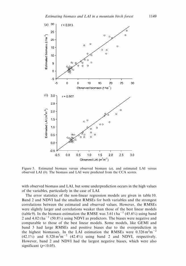
with observed biomass and LAI, but some underprediction occurs in the high values
of the variables, particularly in the case of LAI.
The error statistics of the non-linear regression models are given in table 10.
Band 2 and NDVI had the smallest RMSEs for both variables and the strongest
correlations between the estimated and observed values. However, the RMSEs
were slightly larger and correlations weaker than those of the best linear models
(table 9). In the biomass estimation the RMSE was 3.61 t ha21 (45.6%) using band
2 and 4.02 t ha21 (50.8%) using NDVI as predictors. The biases were negative and
comparable to those of the best linear models. Some models, like GEMI and
band 3 had large RMSEs and positive biases due to the overprediction in
the highest biomasses. In the LAI estimation the RMSEs were 0.326 m2m22
(42.1%) and 0.328 m2m22 (42.4%) using band 2 and NDVI, respectively.
However, band 2 and NDVI had the largest negative biases, which were also
significant (p,0.05).
Figure 5. Estimated biomass versus observed biomass (a), and estimated LAI versusobserved LAI (b). The biomass and LAI were predicted from the CCA scores.
Estimating biomass and LAI in a mountain birch forest 1149

4. Discussion
4.1 Relationship between biomass, LAI and ASTER bands
Red band (band 2) was the single band with the strongest correlation with biomass
and LAI. The chlorophyll pigment in the green leaves absorbs radiation in the red
wavelengths and red reflectance is thus inversely related to the quantity of
chlorophyll present in the canopy (Tucker and Sellers 1986). Furthermore, ascanopy cover increases the amount of sunlit background decreases curvilinearly
decreasing also the observed pixel-level reflectance (Yang and Prince 1997).
Dahlberg (2001) reported that the red bands of the Landsat TM, SPOT XS and
IRS LISS were the best predictors of the biomass and LAI in the heaths and
mountain birch forests in northern Sweden. The high correlations between the red
bands and forest variables has also been observed in the more productive deciduous
stands (Hame et al. 1997, Eklundh et al. 2003) and in the broadleaved stands in the
savannas (Xu et al. 2003). Furthermore, the red band has been among the mostcorrelated bands with the forest variables in the coniferous stands (Spanner et al.
1990, Hame et al. 1997). However, Fassnacht et al. (1997) observed the poor
performance of the red band in the hardwood forests and identified the green band
to be the most correlated band with LAI in the visible range.
NIR band (band 3) showed a strong positive correlation with the forest variables.
In the NIR range the leaf reflectance is high (Tucker and Sellers 1986), whichincreases the canopy reflectance as LAI increases. Dahlberg (2001) found that in the
mountain birch forests the correlation between the NIR bands and LAI was
relatively strong compared to the relationship between NIR bands and biomass. The
direct relationships between NIR bands and forest variables have also been reported
for other types of deciduous stands (Hame et al. 1997, Eklundh et al. 2003), in
contrast to the typically inverse relationships observed in the coniferous stands
(Nilson and Peterson 1994, Hame et al. 1997, Eklundh et al. 2003). Broadleaved
trees with large leaves reflect effectively, but in the coniferous canopies thereflectance is reduced due to increasing multi-layer absorption as the height of the
canopy increases (Hame et al. 1997).
Table 10. Errors and biases of the biomass and LAI estimates predicted by the non-linearregression models, and correlations (r) between the estimated and observed biomasses and
LAIs (n541).
Band orindex
Biomass LAI
RMSE Bias
r
RMSE Biasr
t ha21 % t ha21 % m2 m22 % m2 m22 %
Band 2 3.61 45.6 20.70 28.9 0.904 0.33 42.1 20.13 216.9 0.894Band 3 14.16 178.9 2.85 36.0 0.731 0.73 94.9 0.06 8.3 0.770DVI 6.97 88.1 0.75 9.5 0.815 0.43 55.1 20.04 25.1 0.835NDVI 4.02 50.8 20.36 24.5 0.890 0.33 42.4 20.11 213.7 0.887RDVI 4.84 61.2 0.03 0.3 0.858 0.35 45.5 20.08 210.1 0.865GEMI 12.88 162.8 2.51 31.7 0.746 0.68 87.6 0.05 6.1 0.782MSI 6.42 81.1 0.21 2.7 0.827 0.42 54.0 20.08 210.1 0.837SAVI 5.29 66.9 0.20 2.5 0.848 0.37 47.3 20.07 28.9 0.858OSAVI 4.24 53.6 20.21 22.7 0.874 0.34 43.6 20.09 211.8 0.875SAVI2 7.34 92.8 0.68 8.6 0.839 0.43 56.1 20.06 27.4 0.855MSAVI2 9.56 120.8 1.45 18.3 0.798 0.53 68.0 20.01 21.5 0.826
1150 J. Heiskanen

SWIR band (band 4) had a strong negative correlation with biomass and LAI. This
is in agreement with data from mountain birch forests (Dahlberg 2001) but in
contradiction to the data from other types of deciduous stands (Eklundh et al. 2003).
However, a strong correlation has been found between reflectance in SWIR bands and
forest variables in coniferous stands (Ardo 1992, Eklundh et al. 2003). In the SWIR
wavelengths the reflectance will decrease with increasing leaf area as a consequence of
increasing absorption due to water in the canopies (Tucker and Sellers 1986).
Shadowing is also likely to decrease reflectance in all bands (Ardo 1992).
4.2 Relationship between biomass, LAI and SVIs
The SR was the SVI showing the strongest linear relationship with biomass and
LAI. NDVI had the strongest non-linear relationship, modelled by the exponential
function. Both indices were also strongly correlated with mountain birch biomass
and LAI in the study of Dahlberg (2001). Eklundh et al. (2003) studied the
relationships between several SVIs and LAI in the more productive deciduous
stands and found the strongest correlation between the SR and LAI. Broge and
Leblanc (2000) compared various SVIs using the simulated canopy reflectance data
and the exponential models. They found that the SR and NDVI were the best
indices to estimate LAI at low and medium LAIs. The forms of the relationships are
also in agreement with the results of White et al. (1997).
Several studies have found that SWIR modifications of the SR or NDVI improve
the correlation with LAI in the coniferous forests (Nemani et al. 1993, Brown et al.
2000, Chen et al. 2002, Stenberg et al. 2004) and in the deciduous forests (Chen et al.
2002). However, in the comparison of Eklundh et al. (2003), RSR (which is the
SWIR modification of the SR) performed poorly in the deciduous stands. In this
study RSR showed a strong linear relationship against the forest variables, but
could not enhance the correlation of the SR. The relationship was best described by
the linear model in the range of biomass and LAI values observed in the mountain
birch forest. However, the results of Chen et al. (2002) suggest that the relationship
approaches exponential if higher LAI values occur. NDVIc had a stronger linear
correlation with the forest variables than NDVI, but the relationship with NDVI
was better described by the exponential model. Both RSR and NDVIc are sensitive
to the MIRmin and MIRmax values used (Nemani et al. 1993, Brown et al. 2000),
which is also likely to explain the differences in the model performance in the
different studies.
The soil line adjusted SVIs have been employed successfully in some studies
(Broge and Leblanc 2000). SAVI2 was the best predictor of LAI and the least
affected index by the background reflectance in the sensitivity analysis of Broge and
Leblanc (2000). In this study, SAVI2 had stronger linear relationships in
comparison to other soil line adjusted SVIs, SAVI, OSAVI and MSAVI2, which
were best described by the power law models. The definition of the soil line is
difficult in the forested environment since the bare soil is only rarely visible and soil
line is discontinuous (figure 2).
4.3 Biomass and LAI estimation using CCA scores
The strongest linear relationships in this study were observed between the biomass,
LAI and CCA scores. In the case of biomass, slightly higher R2 values were
produced by some of the non-linear models, but in the case of LAI the linear model
Estimating biomass and LAI in a mountain birch forest 1151
using CCA scores also produced the highest R2 values. According to the error
statistics, the best models for both biomass and LAI were produced by the CCA
scores. CCA provides a method to combine several multitemporal SVIs into a single
index (Cohen et al. 2003), but it was also found to be useful in combining
multispectral data. CCA enables the visual comparison of the single band indices
with the multiple regression analysis, but it also enables the use of the RMA method
in the estimation (Cohen et al. 2003).
The results of the CCA are comparable to the studies employing multiple
regression analysis (Cohen et al. 2003). The results are in agreement with Fassnacht
et al. (1997) who found that multiple-variable models offered substantial
improvement over single-variable models, especially for hardwood stands.
Dahlberg (2001) employed multiple regression models to map biomass and LAI
in the mountain birch forests in northern Sweden. Eklundh et al. (2003) reported
that LAI was modelled most accurately by the multiple regression models of
Landsat TM bands 1, 3 and 4 also in the more productive deciduous stands.
4.4 Effect of the undergrowth vegetation and background reflectance
Several authors have emphasised the effect of the canopy closure, undergrowth
vegetation and background reflectance to the observed relationships between the
reflectance data and forest variables (Badhwar et al. 1986, Spanner et al. 1990,
Nilson and Peterson 1994, Chen and Cihlar 1996, Yang and Prince 1997, Brown
2001). In this study, the canopy closure of the densest plots was estimated from the
hemispherical photographs to be around 50–60%. Therefore, the composition of the
undergrowth vegetation and background reflectance are likely to have a major effect
on the observed canopy reflectance in all the studied plots, particularly in the
sparsest ones.
The dwarf birch (Betula nana) occurred in the bush layer in most of the surveyed
plots. Although the dwarf birch is a shrub (height typically from 0.2 to 0.8 m and
length of the leaves from 0.5 to 1.5 cm), it is known to have spectral properties very
similar to mountain birch (Kayhko and Pellikka 1994). The dwarf birch is most
abundant in the mires but it is likely to have an effect on the observed relationships
and cause overprediction in the stands, where it is particularly abundant.
The spectral properties of the undergrowth vegetation differ according to the
forest types. The undergrowth vegetation is particularly abundant in the sEMT type
where the most important reflectors are the dwarf shrubs, grasses and mosses. This
sort of undergrowth has relatively low reflectance in the red and SWIR bands but
high reflectance in the NIR band (Lang et al. 2002). In the undergrowth of the drier
sELiT type the most important reflectors are lichen and dwarf shrubs, and in the
driest plots the patches of exposed soil, and partly or completely lichen covered
rocks, are common. Contrary to sEMT type, this kind of undergrowth has relatively
high reflectance in the red and SWIR bands and low reflectance in the NIR band
(Lang et al. 2002). The reflectance of the undergrowth vegetation in the sELiPlT
type is somewhere in between these extremes.
Hence, the reflectance of the undergrowth varies similarly to the reflectance of the
mountain birch canopy in a continuum of biomass or LAI values. This will increase
the correlation between the forest variables and reflectance data when data from the
different forest types are combined. This was observed when the correlations of
the pooled data were compared to the correlations stratified by the forest types. The
1152 J. Heiskanen

combined data also included more observations and covered a larger range of
biomass and LAI values, which will increase the correlations (Chen et al. 2002).
The undergrowth vegetation and background reflectance are likely to affect the
strength of the relationship as well as its form. In the lowest biomass and LAI values
the red reflectances were high and NIR reflectances low making the relationships
curvilinear. Furthermore, the sensitivity of the ASTER data to the biomass and LAI
was significantly weaker in the most luxurious sEMT forest type than in the other
forest types. Badhwar et al. (1986) found that the reflectance in all Landsat TM
bands was insensitive to the overstory LAI when understory vegetation was
abundant. In general, the sensitivity of the spectral data to the forest variables is the
highest when the contrast between the background reflectance and canopy
reflectance is greatest (Yang and Prince 1997).
There are also other possible reasons for reduced sensitivity of the spectral data in
the highest biomass and LAI values. Chen et al. (2002) found that, in the deciduous
forests, the SVIs saturate already at LAI values of 2–3 due to multiple scattering
effects. In this study, the reflectance began to saturate already around biomasses of
25 t ha21 and LAIs of 2 m2m22. Furthermore, the low solar elevation angle is likely
to affect the observed relationships. According to the sensitivity analysis of Yang
and Prince (1997), the sensitivity of red reflectance to canopy cover variations is
better with increasing solar zenith angles, but on the other hand the relationship
saturates at lower canopy covers.
4.5 Applicability of the biomass and LAI models
The best models explained around 85% of the variation in the biomass and LAI
values. The lowest RMSEs were 3.45 t ha21 (40.97%) for biomass and 0.28 m2m22
(36.96%) for LAI. The R2 values reported in this study are comparable or higher in
comparison to those previously reported for mountain birch (Dahlberg 2001) and
other broadleaved stands (Chen et al. 2003, Eklundh et al. 2003, Xu et al. 2003).
Generally speaking, the relative RMSEs are also comparable to the other studies,
although Dahlberg (2001) has reported RMSEs as low as 21% and 12% for biomass
and LAI, respectively. Keeping the accuracy of the estimates in mind, the developed
regression models can be employed to estimate biomass and LAI of the mountain
birch stands. The use of linear models is recommended, since non-linear models
could not enhance the reliability statistics.
One reason for relatively good results is that the field plots consisted of only a
single tree species, which is in contradiction to the other types of deciduous stands in
the boreal or temperate zones typically consisting of multiple species (Eklundh et al.
2003). The biomass and LAI values were also relatively low and saturation did not
affect the relationships as much as in the forest types with higher biomass and LAI.
Furthermore, the relatively high spatial resolution of the VNIR bands enabled the
good accuracy in the image rectification.
The most important sources of error and unexplained variation are the variable
undergrowth vegetation and background (discussed above), errors in the biomass
and LAI measurements, and errors in the co-registration of the image data and field
plots. It is important to remember the possible overprediction, due to a high
abundance of the dwarf birch, if the models are employed to predict biomass and
LAI for mountain birch stands. The errors in the surveyed biomass and LAI are due
to measurement errors and local deviations from the employed allometric equations
and SLW value. The co-registration errors were minimised by accurate rectification
Estimating biomass and LAI in a mountain birch forest 1153

enabled by relatively high spatial resolution of the VNIR bands, and by using buffer
zone averaged reflectances instead of pixelwise reflectances.
5. Conclusions
In this study, the potential of the visible to shortwave infrared satellite data for
estimating biomass and LAI in mountain birch forests was examined using ASTER
data. The results showed a strong statistical dependence between the biomass, LAI
and satellite data. This relationship was successfully modelled by CCA and linear
regression analysis. Keeping the accuracy of the estimates in mind, the developed
models are applicable to estimate the biomass and LAI for mountain birch stands,
and will be employed to map biomass and LAI in the study area in the future.
However, the factors affecting the reflectance of mountain birch stands should be
studied further by sensitivity analysis, using a suitable canopy reflectance model.
Particularly, the causes of the saturation in the highest biomass and LAI values, and
the effect of the undergrowth vegetation on the canopy reflectance in a continuum of
canopy closure should be studied. The sensitivity analysis would also provide the
optimal foundation for the selection of the most suitable SVIs for biomass and LAI
estimation in mountain birch forests.
ASTER data have had only a little use in the study of forests. The widespread use
of ASTER is hindered due to relatively small image size and non-systematic data
collection. However, the good spatial resolution of the VNIR bands and spectral
correspondence to the other optical sensors makes it a possible data source for
studying forests. The bandwidths of ASTER are comparable to Landsat TM (or
ETM + ) in the visible and NIR spectral range. Band 4 corresponds to the TM band
5, and relatively narrow bands 5–8 correspond to TM band 7. None of the bands 5–
8 were particularly sensitive to biomass or LAI in the mountain birch forests.
Neither was ASTER band 9, which is outside the TM spectral range. ASTER data is
also provided in the higher order data products, which reduce the effort used in
completing the time consuming and often difficult pre-processing steps by the user
community.
Acknowledgements
The author thanks NASA, METI, ERSDAC and LP DAAC for providing the
ASTER data. The data provided by Metsahallitus was used in the field work
planning and topographic correction. The field work was funded by the Finnish
cultural foundation. Mrs Sonja Kivinen kindly assisted in the field work. Prof. Petri
Pellikka commented on the manuscript and Mr Barnaby Clark checked the
language. Also the comments of the anonymous referees were helpful to finish the
paper.
ReferencesABRAMS, M., 2000, The Advanced Spaceborne Thermal Emission and Reflection Radiometer
(ASTER): Data products for the high spatial resolution imager on NASA’s Terra
platform. International Journal of Remote Sensing, 21, pp. 847–859.
AHTI, T., HAMET-AHTI, L. and JALAS, J., 1968, Vegetation zones and their sections in
northwestern Europe. Annales Botanici Fennici, 5, pp. 169–211.
ARDO, J., 1992, Volume quantification of coniferous forest compartments using spectral
radiance recorded by Landsat Thematic Mapper. International Journal of Remote
Sensing, 13, pp. 1779–1786.
1154 J. Heiskanen

BADHWAR, G.D., MACDONALD R.B., HALL, F.G. and CARNES, J.G., 1986, Spectral
characterisation of biophysical characteristics in a boreal forest: Relationship between
thematic mapper band reflectance and leaf area index for aspen. IEEE Transactions
on Geoscience and Remote Sensing, 24, pp. 322–326.
BIRTH, G.S. and MCVEY, G.R., 1968, Measuring the color of growing turf with a reflectance
spectrophotometer. Agronomy Journal, 60, pp. 640–643.
BROGE, N.H. and LEBLANC, E., 2000, Comparing prediction power and stability of
broadband and hyperspectral vegetation indices for estimation of green leaf area
index and canopy chlorophyll density. Remote Sensing of Environment, 76, pp.
156–172.
BROWN, D.G., 2001, A spectral unmixing approach to leaf area index (LAI) estimation at the
alpine treeline ecotone. In GIS and Remote Sensing Applications in Biogeography and
Ecology, A.C. Millington, S.J. Walsh and P.E. Osbourne (Eds), pp. 7–22 (Boston:
Kluwer Academic Publishers).
BROWN, L., CHEN, J.M., LEBLANC, S.G. and CIHLAR, J., 2000, A shortwave infrared
modification to the simple ratio for LAI retrieval in boreal forests: an image and
model analysis. Remote Sensing of Environment, 71, pp. 16–25.
BROWN, S., 2002, Measuring carbon in forests: current status and future challenges.
Environmental Pollution, 116, pp. 363–372.
BYLUND, H. and NORDELL, K.O., 2001, Biomass proportion, production and leaf nitrogen
distribution in a polycormic mountain birch stand (Betula pubencens ssp.
czerepanovii) in northern Sweden. In Nordic Mountain Birch Ecosystems, Man and
the Biosphere Series 27, F.E. Wielgolaski (Ed.), pp. 115–126 (Paris: UNESCO and
Carnforth: Parthenon).
CHEN, J.M. and BLACK, T.A., 1991, Measuring leaf-area index of plant canopies with branch
architecture. Agricultural and Forest Meteorology, 57, pp. 1–12.
CHEN, J.M. and CIHLAR, J., 1996, Retrieving leaf area index of boreal conifer forests using
Landsat TM images. Remote Sensing of Environment, 55, pp. 153–162.
CHEN, J.M., PAVLIC, G., BROWN, L., CIHLAR, J., LEBLANC, S.G., WHITE, H.P., HALL, R.J.,
PEDDLE, D.R., KING, D.J., TROFYMOW, J.A., SWIFT, E., VAN DER SANDEN J. and
PELLIKKA, P.K.E., 2002, Derivation and validation of Canada-wide coarse resolution
leaf area index maps using high-resolution satellite imagery and ground measure-
ments. Remote Sensing of Environment, 80, pp. 165–184.
COHEN, W.B., MAIERSPERGER, T.K., GOWER, S.T. and TURNER, D.P., 2003, An improved
strategy for regression of biophysical variables and Landsat ETM + data. Remote
Sensing of Environment, 84, pp. 561–571.
COLPAERT, A., KUMPULA, J. and NIEMINEN, M., 2003, Reindeer pasture biomass assessment
using satellite remote sensing. Arctic, 56, pp. 147–158.
CURRAN, P.J. and HAY, A.M., 1986, The importance of measurement error for certain
procedures in remote sensing at optical wavelengths. Photogrammetric Engineering
and Remote Sensing, 52, pp. 229–241.
DAHLBERG, U., 2001, Quantification and classification of Scandinavian mountain vegetation
based on field data and optical satellite images. Licentiate thesis, Swedish University
of Agricultural Sciences, Department of Forest Resource Management and
Geomatics, Report 12.
DAHLBERG, U., BERGE, T.W., PETERSON, H. and VENCATASAWMY, C.P., 2004, Modelling
biomass and leaf area index in a sub-arctic Scandinavian mountain area. Scandinavian
Journal of Forest Research, 19, pp. 60–71.
DREBS, A., NORDLUND, A., KARLSSON, P., HELMINEN, J. and RISSANEN, P., 2002,
Climatological Statistics of Finland 1971–2000, 99 pp. (Helsinki: Finnish
Meteorological Institute).
EKLUNDH, L., HALL, K., ERIKSSON, J., ARDO, J. and PILESJO, P., 2003, Investigating the use
of Landsat thematic mapper data for estimation of forest leaf area index in southern
Sweden. Canadian Journal of Remote Sensing, 29, pp. 349–362.
Estimating biomass and LAI in a mountain birch forest 1155
FASSNACHT, K.S., GOWER, S.T., MACKENZIE, M.D., NORDHEIM, E.V. and LILLESAND, T.M.,
1997, Estimating the leaf area index of North Central Wisconsin forests using the
Landsat thematic mapper. Remote Sensing of Environment, 61, pp. 229–245.
HEIKKINEN, R.K. and KALLIOLA, R.J., 1989, Vegetation types and map of the Kevo nature
reserve, northernmost Finland. Kevo Notes, 8, pp. 1–39.
HELLE, T., 2001, Mountain birch forests and reindeer husbandry. In Nordic Mountain Birch
ecosystems, Man and the Biosphere Series 27, F.E. Wielgolaski (Ed.), pp. 279–291
(Paris: UNESCO and Carnforth: Parthenon).
HUETE, A.R., 1988, A soil-adjusted vegetation index (SAVI). Remote Sensing of Environment,
25, pp. 295–309.
HYVONEN, P., 2002, Kuvioittaisten puustotunnusten ja toimenpide-ehdotusten estimointi k-
lahimman naapurin menetelmalla Landsat TM -satelliittikuvan, vanhan inventointi-
tiedon ja kuviotason tukiaineiston avulla. Metsatieteen aikakauskirja, 3, pp. 363–379
(in Finnish).
HAME, T., SALLI, A., ANDERSSON, K. and LOHI, A., 1997, A new methodology for the
estimation of biomass of conifer-dominated boreal forest using NOAA AVHRR data.
International Journal of Remote Sensing, 18, pp. 3211–3243.
HAMET-AHTI, L., 1963, Zonation of the mountain birch forests in northernmost
Fennoscandia. Annales Botanici Societatis Zoologicae Bonaticae Fennicae ‘Vanamo’,
34, pp. 1–127.
MEYER, P., ITTEN, K.I., KELLENBERGER, T., SANDMEIER, S. and SANDMEIER, R., 1993,
Radiometric corrections of topographically induced effects on Landsat TM data in an
alpine environment. ISPRS Journal of Photogrammetry and Remote Sensing, 48, pp.
17–28.
KAUSE, A., HAUKIOJA, E. and HANHIMAKI, S., 1999, Phenotypic plasticity in foraging
behavior of sawfly larvae. Ecology, 80, pp. 1230–1241.
KULLMAN, L., 2000, Tree-limit rise and recent warming: A geoecological case study from the
Swedish Scandes. Norsk Geografisk Tidsskrift, 54, pp. 49–59.
KAYHKO, J. and PELLIKKA, P., 1994, Remote sensing of the impact of reindeer grazing on
vegetation in northern Fennoscandia using SPOT XS data. Polar Research, 13, pp.
115–124.
LAIDLER, G.J. and TREITZ, P., 2003, Biophysical remote sensing of arctic environments.
Progress in Physical Geography, 27, pp. 44–68.
LANG, M., KUUSK, A., NILSON, T., LUKK, T., PEHK, M. and ALM, G., 2002, Reflectance
spectra of ground vegetation in sub-boreal forests. Available online at: www.aai.ee/
bgf/ger2600/ (accessed 6 September 2004).
MAJOR, D.J., BARET, F. and GUYOT, G., 1990, A ratio vegetation index adjusted for soil
brightness. International Journal of Remote Sensing, 11, pp. 727–740.
MYNENI, R.B., NEMANI, R.R. and RUNNING, S.W., 1997, Estimation of global leaf area index
and absorbed par using radiative transfer models. IEEE Transactions on Geoscience
and Remote Sensing, 35, pp. 1380–1393.
NEMANI, R., PIERCE, L., RUNNING, S. and BAND, L., 1993, Forest ecosystem processes at the
watershed scale: sensitivity to remotely-sensed leaf area index estimates. International
Journal of Remote Sensing, 14, pp. 2519–2534.
NEUVONEN, S., RUOHOMAKI, K., BYLUND, H. and KAITANIEMI, P., 2001, Insect herbivores
and herbivory effects on mountain birch dynamics. In Nordic Mountain Birch
Ecosystems, Man and the Biosphere Series 27, F.E. Wielgolaski (Ed.), pp. 207–222
(Paris: UNESCO and Carnforth: Parthenon).
NILSON, T. and PETERSON, U., 1994, Age dependence of forest reflectance: Analysis of main
driving factors. Remote Sensing of Environment, 48, pp. 319–331.
PINTY, B. and VERSTRAETE, M.M., 1992, GEMI: A non-linear index to monitor global
vegetation from satellites. Vegetatio, 101, pp. 15–20.
QI, J., CHEHBOUNI, A., HUETE, A.R., KERR, Y.H. and SOROOSHIAN, S., 1994, A modified soil
adjusted vegetation index. Remote Sensing of Environment, 48, pp. 119–126.
1156 J. Heiskanen
RANTA, E., RITA, H. and KOUKI, J., 1999, Biometria, 569 pp. (Helsinki: Yliopistopaino) (in
Finnish).
RICH, P.M., 1990, Characterising plant canopies with hemispherical photographs. Remote
Sensing Reviews, 5, pp. 13–29.
ROCK, B.N., VOGELMANN, J.E., WILLIAMS, D.L., VOGELMANN, A.F. and HOSHISAKI, T.,
1986, Remote detection of forest damage. BioScience, 36, pp. 439–445.
RONDEAUX, G., STEVEN, M. and BARET, F., 1996, Optimisation of soil-adjusted vegetation
indices. Remote Sensing of Environment, 55, pp. 95–107.
ROSENQVIST, A., MILNE, A., LUCAS, R., IMHOFF, M. and DOBSON, C., 2003, A review of
remote sensing technology in support of the Kyoto Protocol. Environmental Science
and Policy, 6, pp. 441–455.
ROUJEAN, J.L. and BREON, F.M., 1995, Estimating PAR absorbed by vegetation from
bidirectional reflectance measurements. Remote Sensing of Environment, 51, pp.
375–384.
ROUSE, J.W., HAAS, R.H., SCHELL, J.A. and DEERING, D.W., 1973, Monitoring vegetation
systems in the Great Plains with ERTS. In Third Earth Resources Technology
Satellite-1 Symposium, 10–14 December 1973, Washington, DC (Washington, DC:
NASA), pp. 309–317.
SIHVO, J., 2001, Yla-Lapin luonnonhoitoalueen ja Urho Kekkosen kansallispuiston luontokar-
toitus, pp. 76 (Vantaa: Metsahallitus) (in Finnish).
SKRE, O., 2001, Climate change impacts on mountain birch ecosystems. In Nordic Mountain
Birch Ecosystems, Man and the biosphere series 27, F.E. Wielgolaski (Ed.), pp.
343–357 (Paris: UNESCO and Carnforth: Parthenon).
SPANNER, M.A., PIERCE, L.L., PETERSON, D.L. and RUNNING, S.W., 1990, Remote sensing of
temperate coniferous forest leaf area index. The influence of canopy closure,
understory vegetation and background reflectance. International Journal of Remote
Sensing, 11, pp. 95–111.
STARR, M., HARTMAN, M. and KINNUNEN, T., 1998, Biomass functions for mountain birch in
the Vuoskojarvi Integrated Monitoring area. Boreal Environment Research, 3, pp.
297–303.
STENBERG, P., RAUTIAINEN, M., MANNINEN, T., VOIPIO, P. and SMOLANDER, H., 2004,
Reduced simple ratio better than NDVI for estimating LAI in Finnish pine and
spruce stands. Silva Fennica, 38, pp. 3–14.
TEILLET, P.M., GUINDON, B. and GOODENOUGH, D.G., 1982, On the slope-aspect correc-
tion of multispectral scanner data. Canadian Journal of Remote Sensing, 8, pp.
84–106.
TOMPPO, E., NILSON, M., ROSENBERG, M., AALTO, P. and KENNEDY, P., 2002, Simultaneous
use of Landsat-TM and IRS-1C WiFS data in estimating large area tree stem volume
and aboveground biomass. Remote Sensing of Environment, 82, pp. 156–171.
TUCKER, C.J., 1979, Red and photographic infrared linear combinations for monitoring
vegetation. Remote Sensing of Environment, 8, pp. 127–150.
TUCKER, C.J. and SELLERS, P.J., 1986, Satellite remote sensing of primary production.
International Journal of Remote Sensing, 7, pp. 1395–1416.
TURNER, D.P., COHEN, W.B., KENNEDY, R.E., FASSNACHT, K.S. and BRIGGS, J.M., 1999,
Relationships between leaf area index and Landsat TM spectral vegetation indices
across three temperate zone sites. Remote Sensing of Environment, 70, pp. 52–68.
WARING, R.H. and RUNNING, S.W., 1998, Forest Ecosystems: Analysis at Multiple Scales, 2nd
edition, 370 pp. (San Diego: Academic Press).
WIELGOLASKI, F.E., 1997, Fennoscandian tundra. In Polar and Alpine Tundra, Ecosystems of
the World 3, F.E. Wielgolaski (Ed.), pp. 27–83 (Amsterdam: Elsevier).
XU, B., GONG, P. and PU, R., 2003, Crown closure estimation of oak savannah in a dry
season with Landsat TM imagery: comparison of various indices through correlation
analysis. International Journal of Remote Sensing, 24, pp. 1811–1822.
Estimating biomass and LAI in a mountain birch forest 1157

YAMAGUCHI, Y., KAHLE, A., TSU, H., KAWAKAMI, T. and PNIEL, M., 1998, Overview of
Advanced Spaceborne Thermal Emission and Reflection Radiometer (ASTER).
IEEE Transactions on Geoscience and Remote Sensing, 36, pp. 1062–1071.
YANG, J. and PRINCE, S.D., 1997, A theoretical assessment of the relation between woody
canopy cover and red reflectance. Remote Sensing of Environment, 59, pp. 428–439.
1158 Estimating biomass and LAI in a mountain birch forest