Estimates of poverty ratios and equivalence scales for Russia and parts of the former

USSR

Abstract

The extent of poverty in Russia and the former USSR has been analysed with the

use of relative and subjective poverty lines. Relative poverty lines based on the

distribution of income suggest that poverty has slightly decreased from 1991 to

1995, although income-inequality rose sharply. Analysis based on subjective

poverty lines indicates that some 83% of the Russian households felt poor in 1991,

compared to 78% in 1995. The costs of adults rose sharply while the costs of

children and old age rose slightly during the period.

1 Introduction

In this paper we present comparable estimates for poverty in Russia, Ukraine and

Kazakhstan at the end of 1991 just before the collapse of the Soviet Union and

comparable estimates for Russia in 1993, 1994 and 1995.

We compare two measures of poverty which reflect different ideas as to what

poverty is. We use the relative poverty measures based on the half median and the

half mean income (OECD (1976), Van den Bosch et al. (1993), Flik and Van Praag

(1991)), in which poverty is defined as a relative phenomenon. We also use the

Leyden Poverty Line (LPL: Goedhart et al. (1977)), in which poverty is defined as a

feeling of financial deprivation.

As far as we know, most poverty estimates which have been published for the Soviet

Union and its successors are based on the commodity basket method: this method

produced an estimate of the Russian poverty ratio of 35% in June 1993 (Karasik

(1993)), 24% in December 1993 and 14% in May 1994, although there was no rise

in the real incomes of the poorest 25% of the population during this period (Berger

(1994)). The various estimates given in the Russian press of poverty ratios obtained

1

with the commodity basket method in 1991-1995 even range from 6% to 85%

depending on the institute or authority giving the estimate (Benson (1996)). Apart

from being accused of being politically manipulated (Benson (1996)), these results

are not comparable with those of western countries as there is no reason why the

basket for the Netherlands or France should equal the Russian basket. There are

some estimates of relative poverty for selected regions (e.g. Doyle (1996) and

Gustafsson & Nivorozhkina (1996)). As to subjective poverty, the only study we

know of is that by Milanovic and Jovanovic, who, for the period 1993-1996, analyse

minimum income poverty on a different data set and find similar results to our own.

For pre-transition poverty rates, see e.g. Atkinson & Micklewright (1992). For a

recent survey of poverty analyses and transition issues in Russia see Ellman (1997).

A problem posed by Rose and McAllister (1996), is that the relevance of money for

welfare may be limited in a country like Russia, where part of the production and

trade of goods and services is non-monetized. In our 1991 data set we have self-

reported information on bartering activities and “Unofficial sources of income”

which enables us to estimate their influence on the financial need of households. Our

conclusion is that “unofficial” sources of income make a contribution of about 25%

of total household income in 1991, but that the effect of bartering activities on

financial need was rather small. Unfortunately, such information was not available

for the 1993-1995 surveys. We also find evidence that the importance of money for

the welfare of households has increased over the 1991-1995 period as the economy

has become more monetised.

In section 2 we discuss the poverty line concepts used, where we give particular

attention to the LPL, which has so far mainly been used in Europe, although some

U.S. authors also used subjective measures of poverty (e.g. Vaughan (1993) and

Garner et al. (1996)).

In section 3, we describe the data sets. Section 4 presents estimation results. Section

5 discusses the resulting poverty lines and the transition in or out of poverty. Section

6 concludes

2

2 Relative and subjective poverty lines

In the relative view of poverty, a person is defined as relatively poor when his

income is below a certain percentage of the average or median income. Because

such measures are widely used and are comparable accross countries, we will assess

the degree of half-median and half-mean poverty in Russia and parts of the former

USSR over the transition period. They are however statistical characteristics of the

income distribution and hence they may have nothing to say about the actual level of

financial deprivation in a country.

In the subjective view of poverty, a person is defined to be poor when he feels his

financial resources are inadequate with respect to his needs. It thus accepts

subjectivity explicitly1. We shall use a subjective poverty method known as the

Leyden Poverty Line (LPL) method. It uses questionnaires to determine the level

that people themselves indicate as their poverty line. The respondent is asked to

connect income levels with verbal qualifying labels in terms of “bad income” and

“good income” by the following Income Evaluation Question (IEQ):2,3

"While keeping prices constant, what before-tax total monthly income would

you consider for your family as:

1 We may note that also in the absolute view of poverty, where the ability of a person to buy certain goods or

perform certain tasks decides who is poor, a subjective criterion is indispensable. Even Sen’s definition of the poor as lacking

the capabilities for functionings (Sen, 1983 and 1987) and Townsend's (1979, 1993) definition of the poor as not being able to

"participate in the activities and have living conditions and amenities which are customary, or at least widely encouraged, in

the societies to which they belong", requires a subjectively chosen list of capabilities or activities deemed necessary. The

choice for items deemed necessary in the minimum commodity basket method is also very dependent on the researcher and

the region of research and is hence quite subjective (Callan and Nolan (1991)).

2The Leyden Poverty Line or subjective poverty method was first developed at the University of Leyden by

Goedhart et al. (1977). The IEQ was first developed by Van Praag (1971).

3 The Russian version of this question differs slightly from the wordings mostly used in that income before

taxation was taken instead of after taxation. This latter choice was made since direct taxation was very low in Russia during the

periods investigated.

3

Roubles

very bad,.................................

bad, ........................................

not good not bad,....................

good, ......................................

very good, .............................. "

The five answers of individual i are denoted by c ij. Its log-mean and variance are

denoted by μi and σμ,i2. The predicted value of μi is denoted by μ. The basic approach

is to use household variables such as age, the number of adults (=fsa i), the number of

kids (=fski), and family income (=yi) as predictors of μi and to use (ln(yi)-μ)/σ as an

ordinal household welfare index 4. A household is then called poor if this index falls

below a certain cut-off point. In practice the cut-off point is chosen such that a

household is deemed poor if its household income would be below the expected

income needed to be between a “bad income” and a “not good, not bad income” 5.

For more details on the method, see Hagenaars (1986), Van der Sar et al. (1988),

Van Praag and Flik (1992a), Van Praag (1971, 1994), and Danziger et al. (1984).

The main assumption behind the LPL is that the answers to the normative verbal

labels are meaningful and comparable between individuals. Van Praag (1994) tried

to analyze the meaning of words by asking respondents to place the verbal

qualifications on a straight line between worst and best. Similarly, he asked

4 In the literature on the LPL it is usually argued that the welfare of income is evaluated by Λ(yic;μi,σ) where Λ(.)

stands for the lognormal distribution function. A welfare level of 0.1 then corresponds to an income lower than “very bad”, 0.3

to “bad”, etc. On the functional form see Van Praag (1968), Van Herwaarden and Kapteyn (1981)). Previously it was found,

and also confirmed for the data sets used in this paper, that σμ,i2 is only weakly dependent on his personal characteristics.

Therefore we use the sample average σ2 for interpersonal comparisons (Van Praag (1971), Hagenaars (1986)) and focus on the

explanation of μi.

5An alternative is to ask individuals what is the minimum income ymin they need to make “end meet”. However

this one-level question yields different outcomes. Some people identify it with ‘very bad”, others with “bad” and others with

“barely sufficient”. Hence it confuses all degrees of poverty hardships. The IEQ-multi-level question stabilises the answers and

moreover it is possible to define various levels of subjective poverty by means of the IEQ. A still more simplistic version is the

Gallup-poll question: “what is a minimum income for a representative household of X persons”, where no reference is made to

their own situation and confusion over the meaning of “representative” is likely.

4

respondents to translate the verbal lables into grades between zero and ten. The

verbal labels used in the IEQ-questions appeared to have roughly the same meaning

between members of a language community. Psychological studies also suggest that

normative labels have roughly the same meaning between different language

communities. See Veenhoven (1996) for a review of studies on this issue.

A difference between the LPL and relative poverty lines is in the way they deal with

differences in living conditions accross households, such as family size, growing

one’s own food, the age of the individuals in the household, and whether one owns

the house one lives in or has to rent it. Although all these factors will evidently

influence the income needed to avoid poverty, most of these factors are simply

ignored for relative poverty lines except for the factor household size, say fs, for

which equivalence scales are used. For the relative poverty lines we choose the

customary OECD-scales which counts the first adult as 1, other adults as 0.7 and

children under the age of 18 or those in full-time education as 0.5, even though some

authors have questioned the rigidity and the height of these weights (Van Praag and

Flik (1992a), Van den Bosch et al. (1993)). As is well-known the steepness of the

OECD-scales invariably will yield relatively high levels of poverty in large

families.

By contrast, the equivalence scales used in the LPL are endogenously determined:

the LPL uses equivalence scales which depend on how much extra households

report to need as their family size, age, and bartering activities change (see the

appendix). To assess the difference, we compare the equivalence scales we found for

the LPL with the OECD-scales. An advantage of the LPL is thus that many

different influences on the extent of poverty are taken into account by including

many variables in the explanation of μi.

For a more in-depth review of the (de)merits of different poverty lines, see Callan

and Nolan (1991) and Van Praag and Flik (1992a).

5

3 Data description

This paper uses two household surveys, the Erasmus Survey 1991 and the first three

waves of the Russian National Panel.

The Russian National Panel Survey, a representative survey of households in the

Russian Republic only, was first held in May 1993 and questions 3727 households

on their financial and personal situation6. The response rate in the first wave was

75%. In the second wave 2808 households of the first wave were re-interviewed,

and in the third wave 2273. The panel survey asks respondents for their total income

before taxes from all sources, but not through separate questions like in the

Erasmus-survey. After deleting the cases with missing values, this left 2557 cases

from the first wave, 1904 cases in the second wave and 1444 in the third wave. As

the second and third waves suffered from a significant selection bias towards

households with low reported incomes in the first wave, a weigthing procedure was

used to counter this bias, which is explained in the appendix. We do not include the

results of the 1997 and 1998 waves because of the increasingly high attrition rates

(even though the panel became a revolving panel in 1998), although we mention that

the found poverty results for 1997-1998 remain roughly the same as for 1993-1995.

The Erasmus Household Survey7 was carried out during November and December of

1991 in the republics of Russia, Ukraine and Kazakhstan, where the survey in

Kazakhstan was split up between a survey amongst Russians and non-Russians in

Kazakhstan. Of 10,000 randomly selected households, 8979 households completed a

long questionnaire designed to elicit information on personal finances, personal

living conditions and measures of subjective well-being. An empirical problem with

the measurement of income in 1991 was that income was truncated at 1000 Roubles

6 The Russian National Panel Survey is carried out by the Institute for Comparative Social Research (CESSI) in

Moscow under the guidance of A. Andreenkova and is financed by the Dutch Foundation of Scientific Research (NWO). It

was commissioned and designed by Willem Saris of the University of Amsterdam, whom we thank for allowing us to use the

data-set.

7 The 1991 survey was carried out by the Public Opinion Foundation in Moscow, then headed by Dr. U. Levada.

The survey was designed jointly by B.M.S. Van Praag, Jan Berting and Ruud Veenhoven, all then at the Erasmus University

Rotterdam (EUR). The EUR commissioned the survey and the authors thank the university for making the data set available to

us.

6

per month, which was thought to be a tremendous amount at the conception of the

questionaire. However, due to the rampant inflation at the time of the field work, the

truncation affected 11.7% of the sample. A second problem in the 1991 Erasmus

survey was that only a maximum of two personal incomes were reported for each

household, which, given the prevalence of multi-adult-households, may lead to

serious underestimation of household income for specific cases. The data correction

procedure for both problems is discussed in the appendix. We may note that dealing

with these issues increased income estimates by about 25% from the raw data, but

decreased the poverty estimates only slightly. After deletion of 2668 cases with

missing values, the sample was reweighted to take account of gender, age and

degree of urbanisation. See the appendix for more detailed information.

A more fundamental problem was that just before the collapse of the Soviet Union,

when the Erasmus survey was held in the fall of 1991, inflation was rampant while

incomes lagged behind and the uncertainty with respect to political and economic

development was high. This is reflected by our data, as the amount of money that

was reportedly spent on commodities like food, housing and clothes, exceeded the

total family income by some 21% on average. This unusual feature of the Erasmus

survey may have been caused by large negative savings and/or a severe

underestimation of income. The discrepancy between income and expenditure in

1991 is large enough to doubt whether the reported income did not underestimate

the "true" income for some respondents.

It is obvious that the incomes given by the respondents in the fall of 1991 will be

less reliable, as many people did not know their own income and/or were afraid to

report on it, especially if part of it came from the "unofficial circuit" or if it was

earned as income in kind. Indeed, 48% of households have been reported to be

involved in monetised, but “unofficial” activities (New Russia Barometer (1992)). In

the 1991 data set considerable extra information is available on incomes. First we

asked respondents to quantify their monthly income from three separate sources (cf.

Kapteyn et al. (1988) and Tummers (1994)): income from a main and/or secondary

job (yinc), income from pensions (ypens) and income from "non-declared" activities

(ynon-dec). As un-official income makes up 10% of total reported income on average,

this indicates the existence of unofficial sources. As a control question, the Erasmus-

7

survey posed the following Sources of Income Question (SIQ):

"On a scale of 1 to 5, how important do you regard Source of income x for

your total household budget",

official sources of income, =w1 (w1=1,2,3,4,5)

selling goods on the black market, =w2 (w2=1,2,3,4,5)

exchange of skills and services with others =w3 (w3=1,2,3,4,5)

pensions, grants and allowances =w4

(w4=1,2,3,4,5)

Keeping in mind that all these questions are concerned with income, we can

interpret "Exchanges of skills" as referring to cases where individuals pay each other

for services.

It is obvious that those importance weights give a rough picture of the relative

contributions of sources to total income. More precisely, let us define the following

ratios:

yinc = the income reported for official sources

ypens = the income reported from pensions, grants and allowances

yrep = total reported income, including the part from "undeclared" activities.

The average of A is about 0.9 whereas the average of B is only 0.8, as is the average

of C. As the importance weights are much less exact than filling in exact money

amounts and hence less threatening for the respondent, we may expect that under-

reporting of "grey" income components is present to a much lesser extent when

asking the SIQ. Now consider our basic μ-equation according to which we predict

financial need

B=w1+w4

w1+w2+w4 C=

w1+w2+w4

w1+w2+w3+w4

8

μ=β0+β1ln(ytotal)+β2ln(fsa) +β3ln(1+fsk)+...

We assume that the household income variable the individuals have in mind when

answering the IEQ is not reported income but rather a kind of "total" income,

including non-declared income from black markets and from the exchange of

services between individuals. Now clearly, if everybody would under-report his total

income (ytot) by the same ratio, this ratio would not be separable from the intercept

term in eq. (1). If we however assume that under-estimation varies over individuals,

we can use the ratios A, B, and C to determine the total income. If individuals would

be silent about non-declared black market income, we could correct yrep by a factor

Similarly,

gives an indication of the relative importance of exchange of services for income.

However, the SIQ-questions are rather rough. Hence we specify total income as:

ytotal=yrep×P whereP=( A

BC)

λ

where λ can be estimated from the effect that a higher P will have on financial need.

Clearly, if individuals report their non-declared income correctly, A equals B×C and

P would be 1. If non-declared income is falsely set at zero, A=1, then the correction

for non-reporting is (BC)-λ. λ reflects the degree of information that is added by the

subjective sources of income questions: if the SIQ is completely unreliable, λ=0, and

if the SIQ is completely reliable, λ=1.

Apart from unofficial sources of income, it is also well-known that many Russians

are involved in bartering activities. In order to get some idea of these activities, a

question was included in the Erasmus survey asking for the frequencies of these

activities per month, measured in the variable "barter". We expect, ceteris paribus,

that bartering activities are welfare increasing and would thus reduce financial

needs. We also add a variable for the date of the interview to control for the rampant

inflation in 1991.

(1+w3

w1+w2+w4)

9

4. Estimation Results

In Table 1 we show the determinants of financial needs, i.e., the results for the

regression equations for the 1991 survey together with those for other years.

Table 1: LPL-regressions for USSR 1991 and Russia 1993, 1994, 1995*

___________________________________________________________________________________

USSR(1991) USSR 1991(2) Russia 1993 Russia 1994 Russia

1995

μi μi μi μi μi _____________________________________________________________________________________

__

constant -4.413 (5.61) -4.618 (5.87) 0.51 (0.47) -0.51 (0.44) 0.13

(0.09)

ln(y) 0.403 (34.8) 0.415 (34.6) 0.65 (44.2) 0.63 (39.9) 0.50

(24.6)

ln(fsa) 0.032 (2.08) 0.035 (2.23) 0.12 (4.38) 0.19 (6.65) 0.22

(6.44)

ln(1+fsk) 0.087 (5.15) 0.085 (5.03) 0.08 (2.85) 0.05 (1.81) 0.10

(3.10)

ln(age) 5.004 (11.1) 5.190 (11.6) 2.14 (3.54) 2.97 (4.65) 3.75

(4.85)

ln2(age) -0.709 (11.4) -0.736 (11.9) -0.31 (3.71) -0.42 (4.83) -0.52

(4.96)

Ukraine -0.071 (4.12) -0.070 (4.04)

Kazakhstan (R) -0.099 (3.32) -0.099 (3.29)

Kazakhstan (N-R) -0.104 (4.60) -0.108 (4.11)

date in days 0.002 (4.57) 0.002 (4.61)

ln(bartering in days) -0.015 (1.57)

λ 0.272 (4.84)

R2=0.279 R2=0.273 R2=0.568 R2=0.620 R2=0.501

N=6312 N=6312 N=2557 N=1904 N=1444

_____________________________________________________________________________________

_

*absolute t-values in parentheses

Focussing on 1991(2) first, we find a parameter value for ln(y) of 0.42, which

would mean that a person whose income would increase by 1% would report to need

10

0.42% more in order to reach the same welfare level as before, a phenomenon

termed preference drift in the literature (=β1). This is somewhat lower than the

estimates for many Western countries, but it is in line with poorer Western countries

such as Greece and Spain (Van Praag and Flik (1992b)). For Russia the log-

parabolic effect of age implies that one needs more money when becoming older

until the age of 35, after which one's needs reduce, which is rather standard.

The regional dummies indicate that life in the Ukraine was perceived to be about

0.070/0.58=12% cheaper than in Russia8, while in Kazakhstan one needed about

19% less. However the interpretation of the difference is ambiguous as it is a

combined result of price-level differences and differences in needs between regions.

The coefficient of bartering activities has the expected sign although not as great and

significant as we expected. For somebody involved daily in bartering the measured

effect is a reduction in income needs of about 13%. Obviously bartering every day

seems somewhat extreme, but it suggests that bartering was one way of reducing the

plight of daily life in 1991. What is the effect of the income corrections for

unofficial incomes in 1991? The average value of ln(P) is 0.15, giving an average

relative increase of total income of 14% due to unreported unofficial sources of

income. Adding this “un-mentioned” income to the unofficial incomes which were

reported, we estimate the share of the unofficial monetary economy to be about 25%

of the total economy in 1991, somewhat in line with the findings of Rose and

McAllister (1996, table 1 and 2). This thus affirms the importance of unofficial

sources of income for people to make ends meet. Interestingly enough, variables

denoting whether households grew their own food or had ration vouchers, did not

significantly or substantially influence the level of financial need. Thus despite the

fact that a large fraction of the Russian households is reported to be involved in non-

monetary activities (The New Russia Barometer 1992 estimates the figure at 96% of

households), only bartering activities seem to make an impact on financial need and

not even a very large impact at that.

We may assess the perceived rate of inflation by using an equivalence scale (see

appendix). Using the estimated inflation per day, the inflation rate per year would

be:

8 This number is derived by taking a one-dimensional equivalence scale and equals 0.07/(1-β1). See the appendix

for the derivation of these shadow-prices from equivalence scales..

inflation per year = (y1

y0-1 )⋅100% = (e

0.0018⋅(365-0 )1-0 . 416 -1 )⋅100% = 207%

11

The estimates for the date variable translate into an estimate for annual inflation of

207% in November and December 1991 or about 10% per month, which is much

less than the actual inflation rate of 36% in December 1991 (Kommersant (1991)).

Our subjective estimate however corresponds well to the inflation rate of October,

suggesting a lag of about one to two months in perceived inflation.

For the second data source, the National Russian Panel 1993, there were some

differences with the 1991 data set. First, it covers only the Russian Republic. Hence

we have to omit the regional dummy variables. Second the date variable was found

to be insignificant, probably since the interviews were gathered in the rather short

period of two weeks. Thirdly the SIQ module which we use to construct the income

correction via the variable P was not asked. Average income exceeds average

expenditure by 6% although income was smaller than expenditure for 44% of the

respondents.

Comparing the 1991 results with those for 1993, 1994, and 1995, we see a

substantial increase of R2 from 1991 to 1993 which is probably due to the fact that

individual respondents were completely uprooted in 1991 and had more or less

adapted to the changed situation in 1993. Another aspect will have been that

economic life in 1991 was much more controlled by the state via non-monetary

mechanisms (housing provisions, child-care) than in 1993.

Comparing the 1991 and 1993 income coefficients we see that the preference drift

increased from 0.41 to 0.65 which equals Western values.

A second feature of interest is the change in the age-coefficient. The moment of

greatest financial need increases only slightly from the age of 35 to the age of 37,

but the extent to which old people need less than middle-aged people has decreased

substantially. This perhaps reflects the decreased importance of non-financial

mechanisms for making old age enjoyable such as free-housing, ration vouchers,

and care by children and grandchildren.

Particularly revealing are the large changes that have occurred for the variables of

family size, namely the number of adults and the number of children. As the

coefficients can be interpreted as a measure of the costs of adults and of children, we

12

see a substantial and dramatic increase in the costs of adults: whereas an extra adult

cost virtually nothing in 1991, the second adult in 1993 increases the income needed

by the household to obtain the same welfare level by 35%. We think this signals the

fact that adults in 1991 contributed relatively many goods and services to the

household in a non-monetary fashion and unmeasured ways. For instance, an adult

in 1991 could “pay his keep” by arranging a flat with the local communist party, by

making sure that the family had access to rations and to other state facilities. An

adult in 1995 on the other hand has to “pay his keep” with an income.

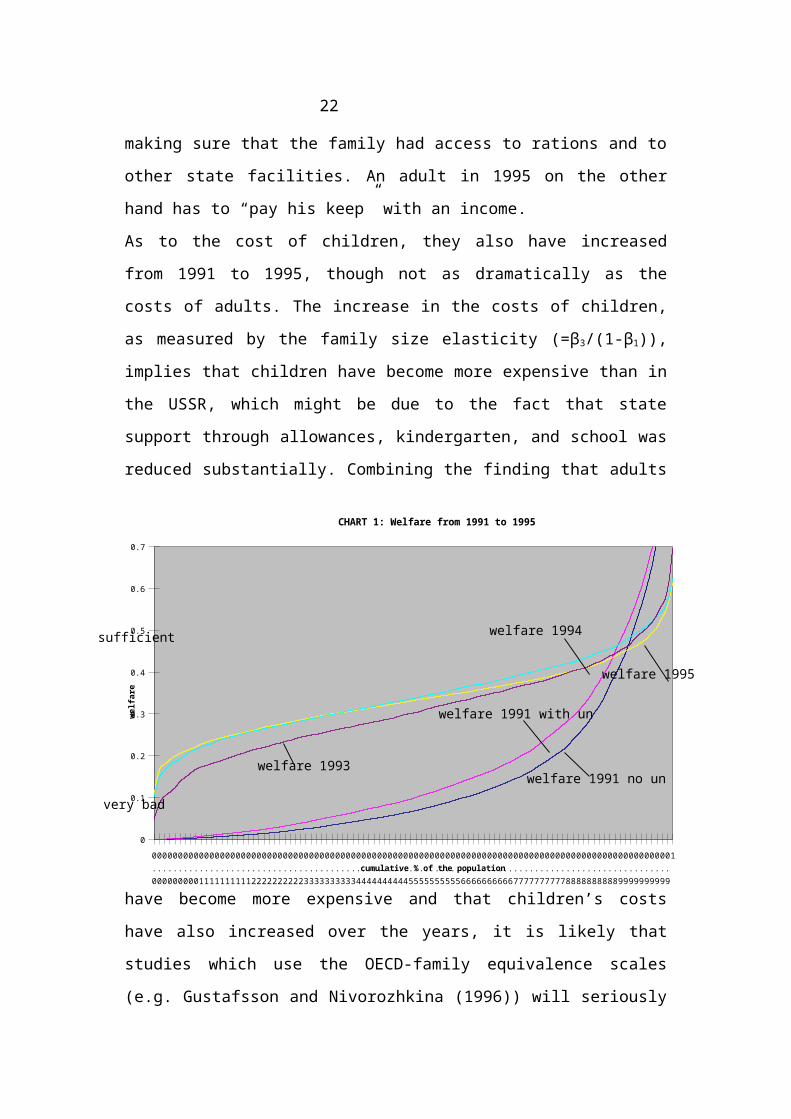
As to the cost of children, they also have increased from 1991 to 1995, though not as

dramatically as the costs of adults. The increase in the costs of children, as measured

by the family size elasticity (=β3/(1-β1)), implies that children have become more

expensive than in the USSR, which might be due to the fact that state support

through allowances, kindergarten, and school was reduced substantially. Combining

the finding that adults have become more expensive and that children’s costs have

also increased over the years, it is likely that studies which use the OECD-family

equivalence scales (e.g. Gustafsson and Nivorozhkina (1996)) will seriously

overestimate the costs of adults in Russia before 1991 and may underestimate them

after 1993.

0.01

0.02

0.03

0.04

0.05

0.06

0.07

0.08

0.09

0.1

0.11

0.12

0.13

0.14

0.15

0.16

0.17

0.18

0.19

0.2

0.21

0.22

0.23

0.24

0.25

0.26

0.27

0.28

0.29

0.3

0.31

0.32

0.33

0.34

0.35

0.36

0.37

0.38

0.39

0.4

0.41

0.42

0.43

0.44

0.45

0.46

0.47

0.48

0.49

0.5

0.51

0.52

0.53

0.54

0.55

0.56

0.57

0.58

0.59

0.6

0.61

0.62

0.63

0.64

0.65

0.66

0.67

0.68

0.69

0.7

0.71

0.72

0.73

0.74

0.75

0.76

0.77

0.78

0.79

0.8

0.81

0.82

0.83

0.84

0.85

0.86

0.87

0.88

0.89

0.9

0.91

0.92

0.93

0.94

0.95

0.96

0.97

0.98

0.99

1

0

0.1

0.2

0.3

0.4

0.5

0.6

0.7

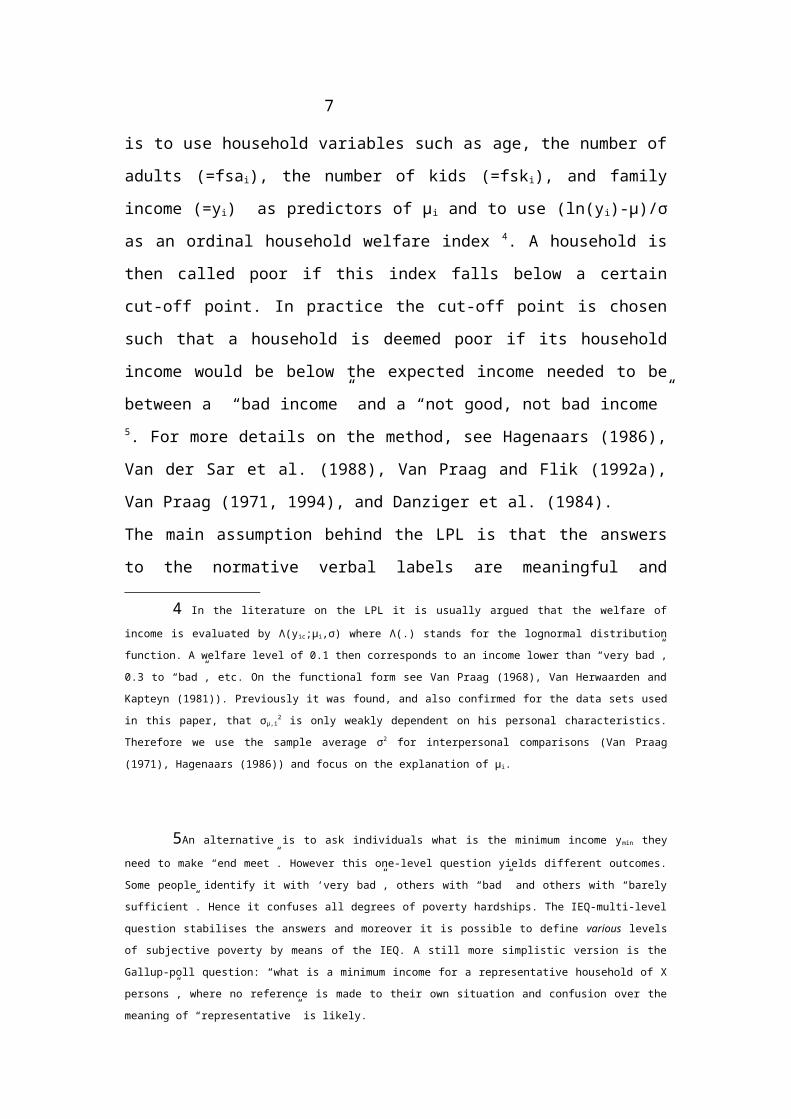
CHART 1: Welfare from 1991 to 1995

cumulative % of the population

wel

fare

welfare 1991 no un

welfare 1991 with un

welfare 1993

welfare 1994

welfare 1995

sufficient

very bad

13

5 Poverty and inequality estimates

First consider Chart 1, which shows the cumulative percentages of individuals below

different welfare levels. Chart 1 shows the outcomes of all four years and shows that

welfare levels (see footnote 4) have increased from 1991 to 1993: for welfare values

which correspond to the range “very bad” and “not good, not bad” (between 0.1 and

0.5), more individuals are better off in and after 1993 than in 1991. As to welfare

after 1993, it seems that the best year was 1994. For a value of γ between 0.1 and

0.45, 1993 had more households living in poverty than in 1995. For welfare values

greater than 0.5, the results are ambiguous.

A striking feature of the welfare distribution in 1991 is the severity of poverty: more

than 70 % of respondents had a welfare lower than 0.15. Thus while the vast

majority of households in all periods considered their own income to be less than

necessary for a “not good-not bad” income, the respondents in 1991 mostly thought

their incomes were worse than “very bad”. As we will see from Table 2, an

important reason for this is that the sample average σμ has increased from 1991 to

1993, which may be viewed as indicating a change in the importance of money in

fulfilling the aspirations of individuals: a small increase in income was sufficient in

1991 to change the judgment of one’s own income from “bad” to “good”. In 1993-

1995 a much bigger increase was needed to achieve the same effect. We think that

the reason for this is the decreased importance of non-monetary mechanisms to

make life bearable after 1991: as housing, child-care and community care all have

become monetised, the increase in σμ simply reflects changing reality (Hagenaars

(1986)). We thus find an increasing importance of money for welfare, contrary to

the findings of Rose and McAllister (1996) who found no relationship between

welfare and income for both 1991 and 1993 in Russia. We suggest this is because

their measure of welfare, labelled as to whether a household was “getting by” or not,

was actually defined as to whether a household’s savings were positive or negative

in 1991 and 1993. As we don’t think positive or negative savings are strongly

related to welfare - savings may simply be related to unanticipated changes in

income and expenditure - we maintain that welfare is increasingly related to

14

household income from 1991 to 1993 and perhaps decreasingly so after 1993.

Chart 1 also shows the difference in welfare for 1991 if we allow for unofficial

sources of income. As can be expected, the inclusion decreases the percentage of

households called poor for all values of γ. However, even after allowing for

unofficial sources of income, poverty still seems to be a lot higher in 1991 than in

1993-1995.

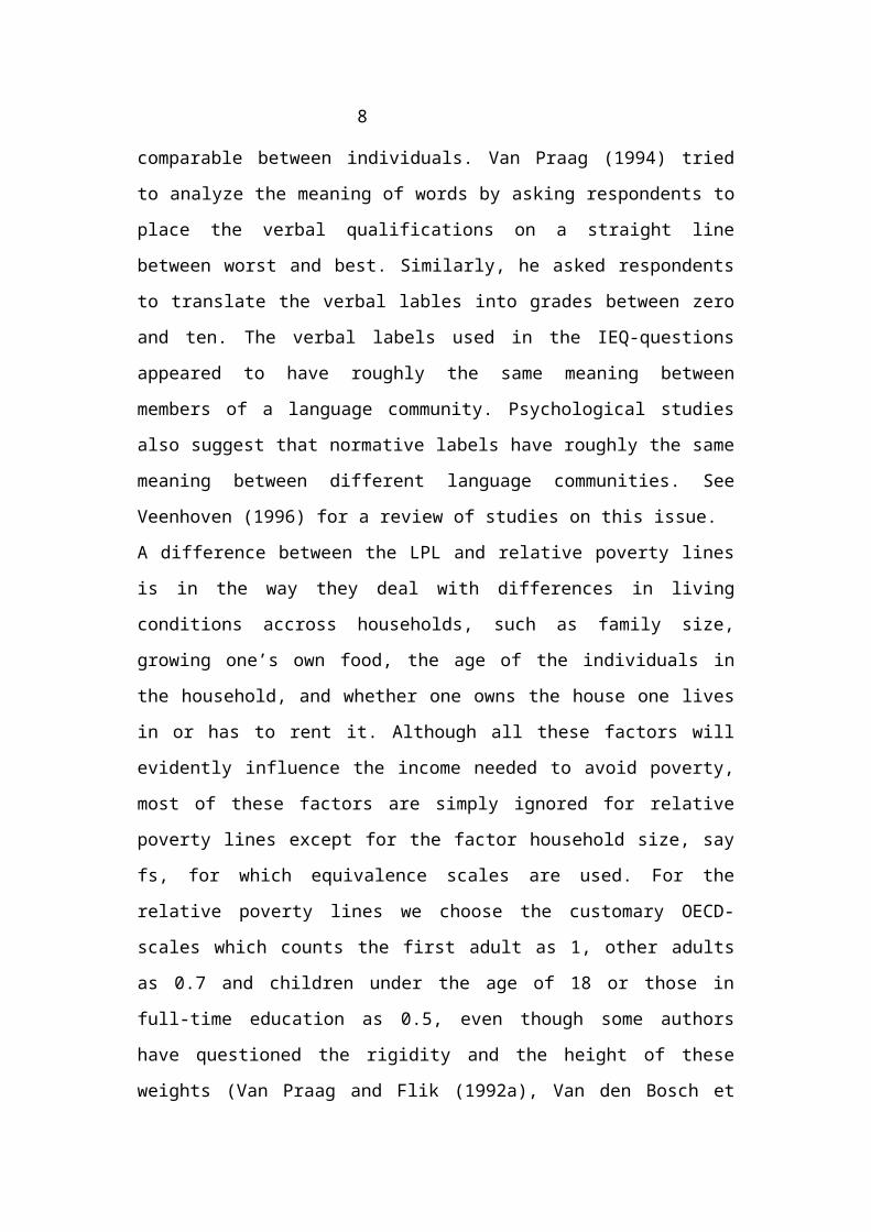
As to relative poverty, the picture changes somewhat, as can be seen from Chart 2,

which shows the cumulative percentage of households whose adult-equivalent

income is below a certain percentage of the mean household income in that year.

Here the picture is not so clear-cut. There seems to be virtually no difference in

mean-related poverty between 1991 and 1993/1994. The only big difference

between the years is that 1995 stands out for having fewer poor people if we draw

the poverty line anywhere between 30% and 80% of mean income. For a poverty

line between 30% and 60% of mean income, poverty is greater in 1993/1994 than in

0.01

0.02

0.03

0.04

0.05

0.06

0.07

0.08

0.09

0.1

0.11

0.12

0.13

0.14

0.15

0.16

0.17

0.18

0.19

0.2

0.21

0.22

0.23

0.24

0.25

0.26

0.27

0.28

0.29

0.3

0.31

0.32

0.33

0.34

0.35

0.36

0.37

0.38

0.39

0.4

0.41

0.42

0.43

0.44

0.45

0.46

0.47

0.48

0.49

0.5

0.51

0.52

0.53

0.54

0.55

0.56

0.57

0.58

0.59

0.6

0.61

0.62

0.63

0.64

0.65

0.66

0.67

0.68

0.69

0.7

0.71

0.72

0.73

0.74

0.75

0.76

0.77

0.78

0.79

0.8

0.81

0.82

0.83

0.84

0.85

0.86

0.87

0.88

0.89

0.9

0.91

0.92

0.93

0.3

0.6

0.9

1.2

1.5

CHART 2: cumulative income distributions 1991-1995

cumulative % of population

Frac

tion

of m

ean

inco

meincome 1991 no unof. incomes

income 1993

income 1994

income 1995

income 1991 with unof. incomes

15

the other years.

Let us consider the outcomes with respect to poverty, when we apply the most

popular cut-off points for the poverty line. This means we compare the half-median,

the half-mean and the LPL measures, where we adopt the welfare level of 0.4 as the

cut-off point and use expected financial need instead of reported financial need. The

results are presented in Table 2, where we apply the customary OECD-family

equivalence scales to the half-median and the half-mean. Poverty estimates for some

European countries (Van Praag and Flik. (1992b), Van Praag et al. (1993), Plug

(1997)) are added for comparison.

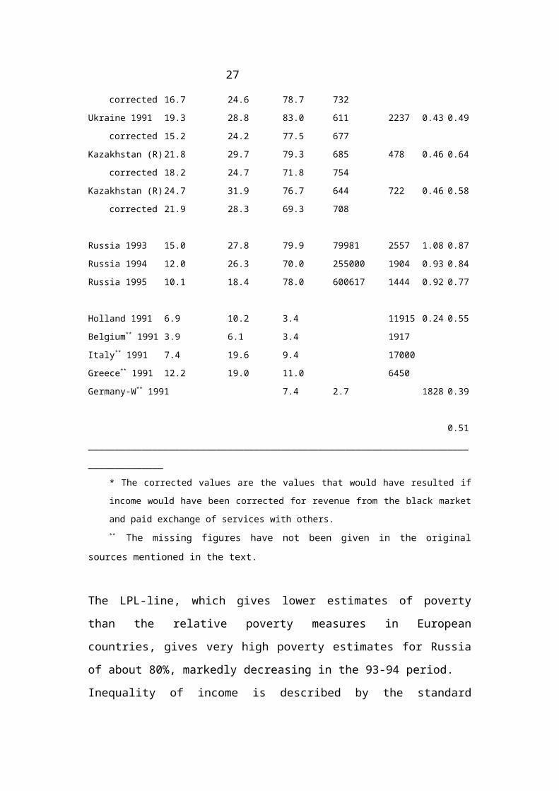
Table 2: Poverty and income inequality in the USSR and in Russia*_____________________________________________________________________________________

__

% poor data characteristics

Half median Half mean LPL average # obs σμ σy

Hous. Income

_____________________________________________________________________________________

__

Russia 1991 19.6 29.9 83.1 661 2875 0.44 0.54

corrected 16.7 24.6 78.7 732

Ukraine 1991 19.3 28.8 83.0 611 2237 0.43 0.49

corrected 15.2 24.2 77.5 677

Kazakhstan (R) 21.8 29.7 79.3 685 478 0.46 0.64

corrected 18.2 24.7 71.8 754

Kazakhstan (R) 24.7 31.9 76.7 644 722 0.46 0.58

corrected 21.9 28.3 69.3 708

Russia 1993 15.0 27.8 79.9 79981 2557 1.08 0.87

Russia 1994 12.0 26.3 70.0 255000 1904 0.93 0.84

Russia 1995 10.1 18.4 78.0 600617 1444 0.92 0.77

Holland 1991 6.9 10.2 3.4 11915 0.24 0.55

Belgium** 1991 3.9 6.1 3.4 1917

Italy** 1991 7.4 19.6 9.4 17000

Greece** 1991 12.2 19.0 11.0 6450

Germany-W** 1991 7.4 2.7 1828 0.39 0.51

_____________________________________________________________________________________

* The corrected values are the values that would have resulted if income would have been corrected

for revenue from the black market and paid exchange of services with others.

16

** The missing figures have not been given in the original sources mentioned in the text.

The LPL-line, which gives lower estimates of poverty than the relative poverty

measures in European countries, gives very high poverty estimates for Russia of

about 80%, markedly decreasing in the 93-94 period.

Inequality of income is described by the standard deviation of log-income, σy. In

contrast with the evolution of the half-mean and half-median lines we see that σy

increased from 1991 to 1993 and decreased somewhat afterwards. The increase in

income inequality between 1991 and 1993 is also born out by the official income

statistics in the Russian Economic Trends (1993, pg. 33) and is analysed further in

Glinskaya and Braithwaite (1999). Furthermore, the correlation between reported

income and unofficial sources of income is -0.13, which shows that the ones most

involved in unofficial income earning are low-income households. Thus while the

rewards of the official economy have increasingly gone to the already well-off, the

poorer individuals are more involved in the unofficial economy.

The finding that the inclusion of unofficial sources of income has benefited the

poorest individuals, is also reflected by a reduction in LPL-poverty of about 8%.

As said before, we interpret the changes in σμ as changes in the importance of money

for the welfare of households. Here an interesting pattern emerges: in 1991 money

was not so important for welfare throughout the USSR, whereas in 1993 money

became much more important. However, from 1993 onwards, the importance of

money has decreased again, as may also be seen from the decreasing R2 and the

decrease in the preference drift variable. It thus seems from these data that

unobserved influences on welfare are again becoming more important.

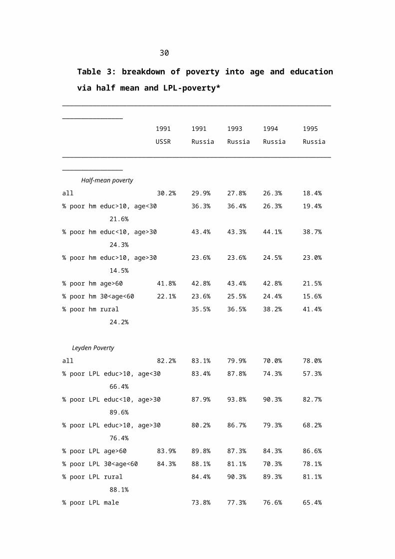
Who is poor?

Table 3 shows the poverty calculations for several subgroups in the data sets in order

to assess the composition of the poor and the aggregate changes:

17

Table 3: breakdown of poverty into age and education via half mean and

LPL-poverty*_____________________________________________________________________________________

__

1991 1991 1993 1994 1995

USSR Russia Russia Russia Russia

_____________________________________________________________________________________

__

Half-mean poverty

all 30.2% 29.9% 27.8% 26.3% 18.4%

% poor hm educ>10, age<30 36.3% 36.4% 26.3% 19.4% 21.6%

% poor hm educ<10, age>30 43.4% 43.3% 44.1% 38.7% 24.3%

% poor hm educ>10, age>30 23.6% 23.6% 24.5% 23.0% 14.5%

% poor hm age>60 41.8% 42.8% 43.4% 42.8% 21.5%

% poor hm 30<age<60 22.1% 23.6% 25.5% 24.4% 15.6%

% poor hm rural 35.5% 36.5% 38.2% 41.4% 24.2%

Leyden Poverty

all 82.2% 83.1% 79.9% 70.0% 78.0%

% poor LPL educ>10, age<30 83.4% 87.8% 74.3% 57.3% 66.4%

% poor LPL educ<10, age>30 87.9% 93.8% 90.3% 82.7% 89.6%

% poor LPL educ>10, age>30 80.2% 86.7% 79.3% 68.2% 76.4%

% poor LPL age>60 83.9% 89.8% 87.3% 84.3% 86.6%

% poor LPL 30<age<60 84.3% 88.1% 81.1% 70.3% 78.1%

% poor LPL rural 84.4% 90.3% 89.3% 81.1% 88.1%

% poor LPL male 73.8% 77.3% 76.6% 65.4% 71.2%

% poor LPL female 88.1% 93.5% 83.9% 74.8% 82.4%

_____________________________________________________________________________________

__

* For comparability, the 1991 results are uncorrected for unofficial sources of income.

For the half-mean we use the traditional OECD scales.

Table 3 shows the percentage of people that are poor within a subset of the total

population. Thus the left top number of 36.4% means that in 1991 in the USSR 36%

of all households with a main respondent younger than 30 and with more than 10

years of schooling earned less than half the mean household income. The table

suggests that in the former USSR relative poverty was mostly concentrated amongst

the lowly educated and the young people, whereas in 1995 the well-educated young

18

persons managed to improve upon their positions. This reversal in position between

the old and the young might be due to the fact that young and highly educated

people have adapted much faster to the new situation.

The same trend holds for the extent to which people feel poor. Older generations

have only become mildly happier with their financial situation, whereas younger and

better educated people have become relatively more satisfied with their income.

Perhaps the younger people have adapted faster to the changing circumstances and

have managed to improve their financial-economic position. These findings closely

mirror those by Gustafsson and Nivorozhkina (1996), who also find in their data set,

based on the Tanarog region, that the old, female and lowly-educated respondents

are more likely to be poor. We also find that rural respondents have remained the

poorest through the transition.

How reliable are the results and what does a poverty ratio of 70% mean?

The high rates of attrition in the panel and the high percentage of respondents with

missing values in both data sets and the many corrections needed to obtain results

are good reasons to view the results with some prudence. Worse, if unofficial

sources of income are also present in 1993-1995, which seems likely, this will bias

our poverty estimates upwards for this period.

First of all though, the results on relative poverty are in line with results found by

others (see e.g. Doyle (1996), Gustafsson and Nivorozhkina (1996)), and the results

on subjective poverty are in line with those found by Milanovic and Jovanovic

(1999), who use an entirely different data set.

Secondly, we may note that each correction to the data set only decreased poverty

ratios. Hence, if we would have included respondents who reported zero incomes or

would have ignored bartering, we would have found an even higher rate of

subjective poverty.

Thirdly, as to whether we underestimate incomes, we may ask how much all

incomes would have to increase such that the Leyden Poverty ratio would have been

only 50%, all else being constant. We find for 1991 that incomes would then have

had to be 120% higher on average and for 1993 that incomes would have had to be

65% higher. Hence, even if the high data attrition and the difficulty in measuring all

19

sources of income would have meant we underestimated incomes by 50% in all

periods, the actual subjective poverty ratio would still have been over 50% of the

population. Therefore the finding that over half the Russian population felt poor

during the period 1991-1995 seems quite robust.

Apart from the assumption that verbal labels are meaningful, the meaningfulness of

our measure of poverty can be assessed by looking at whether the measure

influences the opinion of individuals as to when they were well-off. In Table 4 the

answers are analysed with respect to the question when, according to respondents,

their family was better off.

Table 4: "when was your family better off? Now, during Gorbachow (1985-

1991),

in the former USSR (before Gorbachow) or were there no changes*?"_____________________________________________________________________________

Now Gorbachow USSR No changes

_____________________________________________________________________________

all respondents 12.3% 5.6% 66.4% 11.8%

half-median poor 5.4% 4.4% 78.0% 10.2%

half-mean poor 4.7% 4.2% 79.2% 9.6%

LPL-poor 7.4% 5.3% 73.4% 10.8%

age>60 4.4% 2.2% 79.3% 12.2%

30<age<60 12.9% 5.9% 66.3% 11.2%

age<30 and LPL-not poor 34.5% 8.6% 35.3% 12.1%

age<30 and LPL-poor 12.9% 10.0% 56.5% 13.5%

education<10 years and LPL-not poor 24.5% 6.4% 48.8% 14.4%

education<10 years and LPL-poor 7.4% 5.3% 73.4% 10.8%

rural respondents 8.9% 2.9% 72.2% 12.1%

______________________________________________________________________________

*this question was only asked in the second wave (1994) of the National Panel and thus no trends

can be discerned. As there were a number of respondents in the unsure\don't know category, the

rows do not add up to 100%

Table 4 shows that the poor are more dissatisfied with their present situation than the

rest of the population, who are also quite negative about present times. It does seem

however that younger people are on average much less dissatisfied than others. The

most dissatisfied with present times are the less educated, the old, the rural and the

20

poor according to any definition, which closely mirrors the results from Tables 1

and 3. Whether an individual felt poor mattered significantly for his opinions,

indicating that the LPL is meaningful.

One obvious explanation for the very high subjective poverty ratios is that life is

very hard in Russia. Objective indicators would indeed suggest that in terms of life-

expectancy of males, infant mortality, deseases, incidence of tuberculosis, etc.,

Russia has become comparable to third world countries. Discussing these statistics,

Ellman (1994) therefore speaks of “katastroika”. Real hardship does seem prevelant

in Russia today.

A different explanation is that when Russians answer the question how much

income they need, they are comparing themselves to the richest in their own society,

as the conspicuous consumption of the rich is very visible. Indeed, in 1993, 65% of

the respondents reported to think that their financial position was worse than that of

the average Russian household, with only 6% of respondents thinking their situation

was better. Unbalanced comparisons are therefore also a likely contributor to the

high poverty ratios.

In the conception of poverty as a feeling of deprivation however, the origin of the

feeling does not alter its intensity: regardless of its explanation, over 50% of the

Russian are found to be feeling very poor.

Poverty transition

In a transition period, income and welfare mobility may well be high. Therefore we

look at welfare mobility between years. First we note that as much as 59% of the

respondents were considered to be poor in all three years of the panel according to

the Leyden method. Thus most households who were poor in the 1993 have

remained poor.

Looking more closely at the transition of poverty, we look at welfare mobility in

general. To this effect we calculate the following statistic describing crude mobility:

This defines the mobility of a household as the percentage change a household has

21

mobilityi , tt+1=|rank (ui , t+1 )−rank (ui , t+1 )

N|×100%

made in its ranking within the welfare distribution and hence in the distribution of

Ui=(ln(yi)-μ)/σ. The advantages of this definition of mobility over the standard

measures in the literature, which look at the probability of transition from one

income bracket or welfare bracket to another, are that it is invariant to the definition

of the brackets and the changes in the overall welfare distribution and that each

relative movement, however small, counts. Hence we interpret mobility as a purely

relative concept. If households would be completely mobile, it is easy to see that the

change would be 33% on average.9 As it turns out, the mobility index equals 2.6%

from 1993 to 1994 and 2.3% from 1994 to 1995. This means that mobility is about

8% compared to pure randomness. More interestingly, none of the households in

either year had a higher mobility than 6%, nor is mobility related to the level of

income or poverty in the base year. It thus seems that there are a lot of small welfare

changes from year to year, but no great leaps.

Equivalence scales

In order to compare the effect of the number of adults and children on financial need

between the relative poverty lines and the LPL, we here show multi-dimensional

equivalence scales (see appendix) for Russia for both 1991 and 1995 and compare

them with the values of the OECD equivalence scales.

9

This holds because∫ ¿

0

1

∫ ¿

0

1

|x-y|dxdy= 13

¿¿

This notion of mobility can easily be extended by comparing the empirical average of any m(ui,t,ui,t+1) with its random average.

22

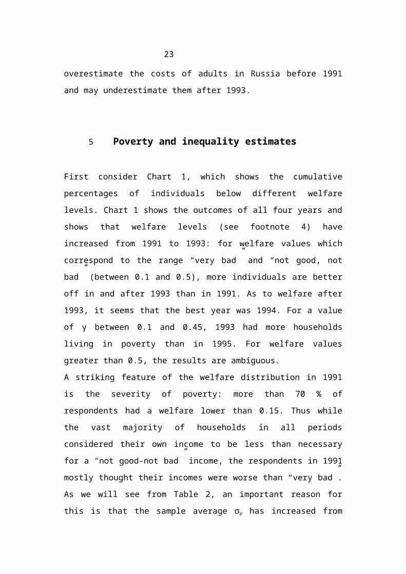
Table 5: Subjective-age-household-equivalence scales for

Russia in 1991 and 1995________________________________________________________________________________

Russia 1991

# adults 1 2 2 2 3 3 4

# children 0 0 1 2 2 3 2

________________________________________________________________________________

Age=25 0.96 1 1.10 1.17 1.20 1.25 1.22

Age=40 1.04 1.09 1.20 1.27 1.30 1.36 1.32

Age=65 0.64 0.67 0.74 0.78 0.80 0.83 0.81

________________________________________________________________________________

Russia 1995 # adults 1 2 2 2 3 3 4

# children 0 0 1 2 2 3 2

________________________________________________________________________________

Age=25 0.74 1 1.15 1.24 1.48 1.57 1.68

Age=40 0.87 1.17 1.35 1.46 1.74 1.84 1.97

Age=65 0.64 0.86 0.98 1.07 1.27 1.34 1.44

________________________________________________________________________________

Table 6: OECD-scales all years________________________________________________________________________________

all ages 0.59 1 1.24 1.47 1.88 2.12 2.29

________________________________________________________________________________

Take for example the figure for a 40 year old Russian respondent with 2 children

and 3 adults in 1991. The figure 1.30 indicates that this family needs only 30 %

more money than a two-adults-no-children household family with a respondent of

25 years to be equally financially well-off (the reference). This rather low figure

probably reflects the support that the state provided for children and pensioners in

1991.

The difference with the OECD-scale is obvious: the effect of age on financial needs

is not reflected by the OECD scales and the subjective perception of costs of adults

and children vary substantially over the period instead of being fixed. Although the

difference is smaller in 1993-1995 than in 1991 or in most other countries, it means

that the LPL finds relatively less poverty amongst households with many children

23

and many adults than the relative poverty lines do. In a sense this reflects intuition:

if having children would make households so poor, why would they have children

anyway (c.f. Pollack and Wales (1979))?

7 Conclusions

The objective of this paper was to get insight into the poverty phenomenon in Russia

and the former USSR, by applying and comparing relative and subjective poverty

measures.

The half median and half mean poverty ratios have decreased slightly during the

transition stage in Russia. As relative poverty is a measure of the shape of the

income distribution, it may not reflect the level of financial hardship in a country.

The Leyden Poverty Line on the other hand, which gives quite conservative

estimates of poverty in the Western-European countries so far examined (Van Praag

and Flik (1992b), Van Praag et al. (1993)), gives us an estimate of poverty of over

70% of the population in all years after 1990. Hence many Russians feel poor, which

is explained by a combination of real hardship and by the fact that most Russians

compare themselves with the richest in their country.

To the extent that poverty has changed over the period 1991-1995, especially the

young and better educated have improved their relative financial and welfare

positions. The estimated increases in the cost of children during 1991-1995 might be

a factor in the drop in the already very low levels of fertility during that period.

Finally we return to the question Rose and McAllister (1996) posed about the

relevance of money for houshold welfare. We presented evidence that the effect of

bartering wasn’t very large in 1991 and that the economy has probably become more

monetised since then. It was also found that welfare influenced the opinions of

individuals about which period was better, the USSR or now. Welfare was indeed

found to matter.

With respect to methodology we see that subjective poverty measurement is

applicable in poor countries, and measures something quite different from relative

poverty.

24

REFERENCES

Atkinson, A.B., Micklewright, J. (1992), Economic transformation in Eastern Europe and the distribution

of income, Cambridge University Press.

Benson, W.E., (1996), “Poverty in the Post-Soviet Russia: myths and realities”, The SSRC Seminar on the

Economics of Transition, St. Petersburg.

Berger, M. (1994), "The Economy", The Current Digest of the Post-Soviet Press, nr. 36, pg. 16.

Blackburn, McKinley L., (1994), "International comparisons of poverty", American Economic Review,

Vol. 84, nr. 2 , pp. 371-374.

Bosch, K. Van den, Callan, T., Estivill, J., Hausman, P., Jeandidier, B., Muffels, R., Yfantopoulos, J.

(1993), "A comparison of poverty in seven European countries and regions using subjective and relative

measures", Journal of Population Economics, nr. 6, pp. 235-259.

Callan, T., Nolan, B. (1991), "Concepts of poverty and the poverty line", Journal of economic surveys,

nr. 5, pp. 243-261.

Coulter, F.A.E., Cowell, A.F., Jenkins, S.P. (1994), "Family fortunes in the 1970s and 1980s", in Blundell,

R., Preston, I. Walker (eds.), The measurement of household welfare, Cambridge University Press, pp.

215-246.

Current digest of the post-Soviet press, The (1994), nr. 28, pg. 8.

Danziger, S., Van der Gaag, J., Taussig, M.K., Smolensky, E. (1984), “The direct measurement of welfare

levels: how much does it cost to make ends meet?”, Review of Economics and Statistics, 66, pp. 500-505

Doyle, C. (1996), “The distributional consequences during the early stages of Russia’s reform”, Review of

Income and Wealth, no. 4, pp. 493-505.

Ekonomika _izn' (1994), nr. 7, pg B04.

Ellman, M. (1997), “The political economy of transformation”, Oxford Review of Economic Policy, 13(2),

pp. 23-32.

Ellman, M. (1994), “The increase in death and desease under ‘Katastroika’”, Cambridge Journal of

Economics, 18(4), pp. 329-355.

Flik, R.J., Van Praag, B.M.S., (1991), "Subjective poverty line definitions", De Economist 139, nr 3., pp.

311-330

Foster, J.E., Shorrocks, A.F., (1988) "Poverty orderings" Econometrica, nr. 56, pp. 173- 177.

Garner, T.I, Stinson, L., Shipp, S., (1996), “Subjective assessments of well-being”, a paper presented at the

1996 meeting of the American Statistical Association.

Glinskaya, E., Braithwaite, J. (1999), “Poverty, inequality, and income mobility in Russia 1994-1996”,

American Population Association Paper, forthcoming.

Goedhart, T., Halberstadt, V., Kapteyn, A., Van Praag, B.M.S. (1977), "The poverty line: concepts and

measurement", Journal of Human Resources, nr. 12, pp. 503-520.

Gustafsson, B., Nivorozkina, L., (1996), “Relative poverty in two egalitarian societies: a comparison

between

25

Taganrog, Russia during the Soviet era and Sweden”, Review of Income and Wealth, no 3, pp. 321-334

Hagenaars, A.J.M., (1986), The perception of poverty, North-Holland, Amsterdam.

Herwaarden, F.G van, Kapteyn, A. (1981), "Empirical comparisons of the shape of welfare functions",

European economic Review, pp. 261-286, nr. 15.

Kapteyn, A, Kooreman, P. and R. Willemse (1988), "Some methodological issues in the implementation

of subjective poverty definitions", The Journal of Human resources, vol. 2, nr. 23, pp. 222-242.

Karasik, T.W. (1994), Russia & Eurasia. Facts and Figures Annual, Academic International Press, pg. 71.

Kommersant (1991), nr. 49, pg. 8.

Lewbel, A. (1989), “Household equivalence scales and welfare comparisons”, Journal of Public

Economics,

vol. 39, pp. 377-391

Milanovic, B., Jovanovic, J. (1999), “Change in the perception of the poverty line during the times of

depression: Russia 1993-1996”, mimeo.

Moscow News (1994), nr. 27, pg. 8.

OECD (1976), "Public expenditure on income maintenance programmes", Studies in Resource

Allocation, nr 3, Paris.

OECD (1982), The OECD list of social indicators, Paris.

Plug, E.J.S. (1997), Leyden welfare and beyond, Thesis Publishers, Amsterdam

Pollak, R.A., Wales, T.J., (1979), "Equity: the individual versus the family. Welfare comparisons and

equivalence scales". American Economic Review, 69, pp. 216-221.

Rose, R., McAllister, I.(1996), “Is money the measure of welfare in Russia?”, Review of Income and

Wealth,

no 1, pp. 75-90.

Sen, A.K. (1983), "Poor, relatively speaking", Oxford Economic papers, nr. 35, pp. 153- 169.

Sen, A.K. (1987), The standard of Living, Cambridge University Press, The Tanner Lectures.

Townsend, P. (1979), Poverty in the United Kingdom, Harmondsworth, Penguin.

Townsend, P. (1993), The analysis of Poverty, Harvester/Wheatsheaf.

Tummers, M.P. (1994), "The effect of systematic misperception of income on the subjective poverty line",

in Blundell, R., Preston, I. Walker, I. (eds.), The measurement of household welfare, Cambridge

University Press, pp. 265-274.

Van der Sar, N.L., Van Praag, B.M.S., Dubnoff, S., (1988), "Evaluation questions and income utility",

in B. Munier (ed.), Risk, decision and rationality, Dordrecht, Reidel Publishing Co., pp. 77-96.

Van Praag, B.M.S. (1968), Individual welfare functions and consumer behaviour. A theory of rational

irrationality, Phd-thesis, North-Holland Publishing Company, Amsterdam.

Van Praag, B.M.S. (1971), "The welfare function of income in Belgium: an empirical investigation",

European Economic Review, nr. 2, pp. 337-369.

Van Praag, B.M.S. (1994), "Ordinal and cardinal utility: an integration of the two dimensions of the

welfare concept", in Blundell, R., Preston, I. Walker, I. (eds.), The measurement of household welfare,

Cambridge University Press, pp. 86-110.

Van Praag, B.M.S., Spit, J.S., Van de Stadt, H., (1982), “A comparison between the food ratio poverty line

and the Leyden poverty line”, Review of economics and Statistics, 64(4), pp. 691-694.

26

Van Praag, B.M.S., Flik , R.J. (1992a), "Poverty lines and equivalence scales. A theoretical and empirical

investigation", Poverty measurement for economies in transition in Eastern Europe, International

Scientific Conference, Warsaw, 7-9 October, Polish Statistical Association, Central Statistical Office.

Van Praag, B.M.S., Flik , R.J. (1992b), "Subjective poverty", Foundation for Economic Research

Rotterdam, Research Institute for Population Economics, Final Report in the Framework of the Eurostat

Project "Enhancement of family budget surveys to derive statistical data on least privileged groups".

Van Praag, B.M.S., Bispo A., Stam, P.J.A. (1993), Armoede in Nederland, Ministerie van Sociale Zaken

en Werkgelegenheid, Den Haag: VUGA Uitgeverij B.V.

Van Praag, B.M.S., Warnaar, M.F. (1997), “The costs of children and the use of demographic variables in

consumer demand”, in Rosenzweig, M., Stark, O. (Eds), The Handbook for population and family

economics, vol 1A, pp. 241-273. North Holland Publishing.

Vaughan, D.R. (1993), “Exploring the use of the public’s views to set income poverty thresholds and

adjust

them over time”, Social Security Bulletin, vol 56(2), pp. 3-25

Veenhoven, R. (1996), ''Happy life-expectancy: a comprehensive measure of quality of life in nations'',

Social

Indicators Research, 39, pp. 1-58.

Appendix

A1: Income in the Erasmus-data set.The Erasmus-data set consisted at first of 8979 cases. After deletion of those members with missing age, family size, IEQ or date, 7075 cases were left. Weights were constructed such that the sample distribution of regions, age, education, marital status and urbanisation was the same as in the 1989 census.Then income was looked at. Income was measured by asking the main respondent and, if appropriate, a resident partner to report their income for the following four sources: 1. Income from a primary job2. Income from another, official job3. Income from allowances, pensions, insurance, etc.4. Income from non-declared activities

Each case thus consists of 8 income variables. As the male income from any source was significantly higher than that of a female, the first step was to group our information into 8 variables: two variables per source of income, one male, one female. Two problems had to be overcome: truncation and missing incomes in the case of more than 2 household-income earners. First we deal with the truncation problem.Income was truncated at 1000 roubles to avoid non-response and had to be estimated for those incomes above the truncation level. To illustrate how this was done, consider the male income from a primary job (4772 cases). A tobit analysis was done and the income regression read:

ln(ymale, primary job)= 4.23 + 0.0086×ln(age) - 0.000000015×ln2(age) + 0.582×ln(education in years)t-values (33.7) (12.6) (10.2) (12.1)

Non-truncated cases = 4555Truncated cases = 217Log-Likelihood = -3982.685Normal scale parameter = 0.545

A truncated income was then estimated by taking a random draw from the individually determined truncated

27

distribution. This procedure was done for both sexes for income sources 1, 2 and 4. Income from pensions and allowances was not only truncated in less than 20 cases, but was also very far off the mean pension level (about 140) and no reliable separate analysis could be done for this category: pensions at the truncation level were set at 1000. Imputations reduced estimates of half-mean poverty but hardly affected the other methods.The second problem was that we did not have the income available of other adults living in the households in 1991. This meant that only two incomes were recorded of households with 2 or more incomes. As 25% of the households in 1993 had more than 2 income-earners, this could be expected to present a serious problem which would seriously bias the poverty estimates upwards. To deal with this problem, we wrote household income as the sum of probable incomes:

ynri,i equals household income, y1ri,i equals the income of the first respondent, P1991[nri=j|Xi] denotes the probability that the household has j income earners, given its characteristics X. The first part of this equation merely re-writes income as the product of a ratio and the income of the first respondent. The second part writes this ratio as the sum of probabilities (which are zero for all values of j other than nr i and one if j equals nri) times ratios. Our “trick” is to replace the unknown P1991 and R1991 by P1993 and R1993 . We thus calculate for all households in 1991 how many income-earners they were likely to have given their number of resident adults, their first income, the age of the first respondent and their answer to the IEQ-question, and we calculate the expected ratio of the total household income to the income of the first respondent, given the number of household earners, the income, and the age of the respondent. For P1993 we used an ordered-probit procedure with the number of adults, the age of the respondent and the relative financial need of the household as explanatory variables. R1993 was estimated for each number of income earning adults as a simple linear function of the relative age of the household and the relative income of the first respondent. The latter variable was significantly negatively related to the income ratio. This may be expected for if the first respondent is in the bottom of the income distribution for first respondents, the other income earners in a house will probably do relatively better. The higher the age of the first respondent, the lower the income ratio was (thus the more important the income of the first respondent to the whole of household income).We then insert for each household a random draw of the number of household earners given their characteristics in 1991 and multiply the income of the first respondent with the expected ratio. This whole procedure increased average household incomes by about 15%. A problem arising out of the way in which we dealt with truncation and missing incomes is that we introduced extra variation in household income. This would normally bias the OLS-estimate of the variable household income down by a ratio of (σ2

y+σ2e)/(σ2

y) in which σ2y denotes the true

variance of income and σ2e the added variance. By numerically estimating (σ2

y+σ2e)/(σ2

y) to be 1.117 we corrected the OLS-results for this bias. This procedure reduced all estimates of poverty. As the imputation depends on the assumption of a constant relationship, their reliability is unknown.

A2: ad-hoc assumptions in recoding the Erasmus-data set:

1. Bartering activity was measured by asking how often one participated in bartering activities. The answers were then recoded according to the following rule:"practically each day" = 30 times per month"one time a week or more" = 10 times per month"one time a month or more" = 2 times per month"very seldom" = 1 time per month"sometimes" or "no answer" = 1 time in every two months

2. It can occur that people fill in their yearly income when they are asked to fill in their monthly income. Although the effects were not that great, this had to be corrected. We assumed that this was the case when both the following conditions were met (8 cases):a. Reported income was greater than 1600 (whilst average income was 600).b. Income was found to be more than four times greater than what they considered to be a good income.

28

ynri ,i = Σj=1

M

I nri=j¿

ynr i ,iy1r,i

¿ y1 r i ,i= Σ

j=1

M

P1991[ nri =j|X i]⋅R1991( Xi)⋅y1 ri ,i

3. It can occur that people fill in their perception of what constitutes a good/bad/so-so yearly income when answering the Income Evaluation Question in the wrong way. We assumed that this was the case if the following two conditions were met:a. total family income was greater than 100 (an absolute minimum income)b. a "very bad" income was more than 3 times the total family incomeInstead of recoding these cases we could also have deleted them, which would have served our overall variance better (it could well be that this method has identified people who did not take the questions seriously instead of those being mistaken about the period involved). This held for 351 cases.

4. There were a number of cases whose reported total family income from all sources was less than 10 roubles per month. 10 Roubles per month wouldn't have bought a loaf of bread in December 1991 and thus these cases (94 cases) were deleted on the grounds that one could not take these answers seriously. Apart from this, there were 642 cases with missing or zero incomes.

5. Persons who answered the IEQ-questions in the wrong way, who claimed that to them a "good" income was a lower income than a "bad" income, were not deleted but their answers were reversed. This happened in 40 cases.

6. The variable "family size" was assumed to be equal to the answer to the following question: "What is the total amount of people in your household?"

7. All people answering the questions of age, IEQ and number of household members with "don't knows" or "refuse to answer" were deemed to be missing values (it is in fact not possible to ascertain now whether these persons actually had answered in this way or that a missing value was coded in this way). If no source of income was reported at all (not even an income of 0), a missing value was assumed. Whenever one of the IEQ-answers was missing, a missing value was reported for μ (after deletion of all other missing values: 26 cases), although later analysis showed that computing the values via interpolation wouldn't have significantly altered our results.

8. The variable expenditure referred to in the text is defined as the sum of monhly expenditures on the following items: water, gas, electricity, housing, telephone, schooling, taxes, insurance, childcare, food, drinks, clothing, cars, public transport, sigarettes, tobacco, entertainment and vacations.

A3: ad-hoc assumptions regarding the 1993\4\5 panel data sets:1. It can occur that people fill in their yearly income when they are asked to fill in their monthly income. The criteria that were used for the Erasmus-data set were however almost never met for this data set (first wave: 4 cases, second wave: 3 cases, third wave: no cases), indicating perhaps the greater familiarity with surveys of this kind.

2. It can occur that people fill in their perception of what constitutes a good/bad/so-so yearly income when answering the Income Evaluation Question. This did not occur often in the Panel Survey. We assumed that this was the case if the following two conditions were met (first wave: 78 cases, second wave: 47 cases, third wave: 0 cases):a. total family income was greater than 1000 (an absolute minimum income)b. a "bad" income was more than 5 times the total family income.

3. The family size was assumed to be equal to the answer to the following question: "How many people, including you, live in your family now?".

Note that this is not exactly the same wording as in the Erasmus survey. The difference is assumed to be small and unimportant.

4. All people answering the questions with respect to age, IEQ and the number of household members with "don't knows" or "refuse to answer" were deemed to be missing values (it is in fact not possible to ascertain now whether these persons actually had answered in this way or that a missing value was coded in this way). If no source of income was reported at all (not even an income of 0), a missing value was assumed. Whenever one of

29

the IEQ-answers was missing, a missing value was reported for μ, although later analysis showed that computing the values via interpolation wouldn't have significantly altered our results. Number of missing values: 4.a. age: 0 in both waves4.b. family size: 0 in both waves4.d. μ 688 in the first wave, 507 in the second, 635 in the third4.e. family income 481 in the first wave, 397 in the second, 194 in the third

5. In order to counter a possible selection bias, we have reweighted all three waves so that the sample distributions of the respondents in the three poverty analyses for 1993, 1994 and 1995 are equal to the sample distribution of all the respondents of the first wave, including those with missing values for income or μ. The reweighting was performed for the 1993 variables of age, education, family size and expenditure. If any of these variables was missing, a dummy was included. Probit-equations were run to determine the probability of being included in the sample. The reference group were all the 3727 persons in the first wave. Weights were then constructed from the inverse of the found probabilities of selection. The weights were normalised to 1. Hence we allowed for selection on the mentioned observed 1993 variables. We could not counter selection on unobservables.

6. In computing the amount of poor people for 1994 and 1995 in table 2, there was the problem that our sample had got older and a bit better educated, whereas the population as a whole hadn't. In order to obtain an accurate estimate for poverty, those figures in table 3 denoting the distribution of poverty over specific education and age groups were used: the relative frequencies of poverty amongst different age and education groups in 1994 and 1995 were multiplied with the percentages of people within those groups in 1993 to obtain the poverty estimates for 1994 and 1995. Let Px(agei,educj) denote the percentage of poor people within the joint age group i and education group j in year x. If Fy(agei,educj) denotes the percentage of the total population that fall in the group with age i and education j in year y, then 1994 poverty becomes:

Using only the three income-age groups of table 3 reduced 1994 and 1995 poverty estimates by less than 2% and a procedure with more possible combinations of age and education was tried but gave the same results.

A4: Overall remarks on the two data sets.Of those who did not declare their family income in the 1993\4\5 surveys, some 50% did indicate which interval their income lay. The average income did not differ more than 5% for those people, thus we assume that the omission of those who did not fill in any monetary income did not affect the results in significant ways. Hence the net loss due to missing values is only about 50% of deleted for non-response to the continuous income question. It must be noted that in all three surveys, the deletion of missing μ and family income variables did not significantly affect the average household composition, hours spent at work, age or gender of the sample. As far as deleting those with very low incomes (zero or near zero) is concerned, this will only bias the poverty results downwards.The results for the Erasmus-survey were re-estimated with the use of weights which did not have a greater than 2 % effect on any of the variables in tables 1 and 4. The only recoding assumption that thus makes a big difference for the results is the recoding of very high answers to the IEQ-questions in the Erasmus-data set (although even that is not able to affect the number of people counted as feeling poor very much, though it radically affects the IEQ-coefficients). This relative robustness of the Leyden Poverty Line is also apparent if we do not estimate μ(yic), but merely compute the utility from each household's income directly by using the IEQ-answers and the log-normality assumption. In that case the overall LPL-poverty results still do not change more than 10% absolutely and all the relative comparisons still hold.

A5: Leyden equivalence scales.If one household experiences a welfare level γ with an income y0 , we would be interested in the income y i that a

30

Poverty1994 = Σi=1

n

Σj=1

m

P1994(age i , educ j )⋅F1993( agei , educ j )

household with different characteristics would have to receive to experience the same welfare. These equivalence scales are constructed by equating the welfare levels of different households and solving for income. For the reference household (household "0"), a two-person household with a respondent of age 25, living in region 1 (Russia) has been chosen. Note that the equivalence scales do not depend on average income or what is considered to be the minimum welfare level. It can be shown that two households 0 and i derive equal welfare from their respective incomes y0 and yi when

ln(y0c) - μ0(y0c) - σμN-1(γ) = ln(yic) - μi(yic) - σμ N-1(γ)

which follows when the Leyden welfare of an income is assumed equal to Λ(y ic;μi,σ). The specification is unimportant as it drops out. When µi=β0+β1ln(yic)+β2ln(fsai)+β3ln(1+fski)+β4ln(agei)+β5ln2(agei)+β¢Ci+εi we have

With C a vector of variables of interest.

Note that by its functional specification this is a multiplicative Independence of Base scale (Blackorby and Donaldson (1994) or Lewbel (1989)).

31

ln (y ic

y0c)=

β2 ln (fsai

fsa0)+β3 ln (

1+ fski

1+ fsk0)+β4 ln(

agei

age0)+ β5 ln2( agei )−β5 ln2(age0 )+ β' (C i−C0 )

1- β1