estimated regional wage relativities for england a …blnchflr/papers/4975.pdf · estimated...

February 2002

Estimated Regional Wage Relativities for EnglandA Report for the South East Area Cost AdjustmentGroup & Association of London Government

Dr. David Blanchflower, NERA Special Consultant

Andrew Oswald, Professor of Economics, Warwick University

Brian Williamson, NERA Senior Consultant

TABLE OF CONTENTS

EXECUTIVE SUMMARY I

1. INTRODUCTION 1

2. CONTEXT & METHODOLOGY 2 2.1. Summary 2 2.2. The Underlying Problem 2 2.3. Context & Alternative Approaches 3 2.4. Our Approach 6

3. EMPIRICAL RESULTS – LABOUR FORCE SURVEY 8 3.1. Summary 8 3.2. Public & Private Sector Weekly Wage 9 3.3. Private Sector Weekly Wage 11 3.4. Public & Private Sector Hourly Wage 11 3.5. Private Sector Hourly Wage 11

4. EMPIRICAL RESULTS – NEW EARNINGS SURVEY 12 4.1. Summary 12 4.2. Public & Private Sector 13 4.3. Private Sector 13 4.4. Public & Private Sector Using Fixed Effect Method 13 4.5. Private Sector Using Fixed Effects 15 4.6. Further Analysis of Movers 15

5. SENSITIVITY ANALYSIS 17 5.1. Summary 17 5.2. Sensitivity to Occupational Grouping 17 5.3. Sensitivity to Time Period 18 5.4. Sensitivity to Level of Regional Aggregation 19 5.5. Further Sensitivity Analysis 19

6. CONCLUSIONS 20

APPENDIX A. THE DATA SETS 21 A.1. Labour Force Survey 21 A.2. New Earnings Survey 22 A.3. Implications of Underlying Income Distribution 23

APPENDIX B. EMPIRICAL RESULTS 26

APPENDIX C. AREA CODES 37

APPENDIX D. OCCUPATIONAL CODES 43

APPENDIX E. FIXED EFFECTS & EARLIER RELATED WORK 44

REFERENCES 48

www.nera.com i

EXECUTIVE SUMMARY

The South East Area Cost Adjustment Group and Association of London Government commissioned NERA to estimate regional wage relativities for England. The context for the work is the question of how central government funding of local authorities should be adjusted regionally to allow delivery of equivalent levels of service.

We examine how to adjust funding for local authority services for differences in the price of labour inputs across regions. The intent of funding adjustments for relative input prices and volumes (or needs) is to ensure that all local authorities have the same potential to deliver services of a given quality (for the same level of local council taxpayer input). We focus on what the relative regional adjustment for differences in labour costs ought to be. We do not comment on the appropriate aggregate level of funding. Nor do we comment on how regional funding should be adjusted to reflect local needs.

The approach we adopt is to examine regional wage differentials revealed by labour market statistics (the general labour market approach). To isolate the impact of region alone on regional wage relativities – to ensure a like-with-like comparison - we control statistically for factors such as the composition of the workforce and occupations region by region. Our preferred approach rests on analysis of a sample of private sector workers – since using existing public sector wage differentials to decide what public sector funding ought to be would be circular. We are interested in uncovering the correct regional pay relativities.

We consider both New Earnings Survey (NES) and Labour Force Survey (LFS) data. We argue for estimates based on the LFS since the NES excludes many of the low paid (those not required to file income tax returns) – thereby biasing downwards-estimated regional wage relativities. Another reason for preferring the LFS is that the sample data includes, and allows us to “control for”, information on worker characteristics such as qualifications.

We argue that it is crucial to use private sector relativities in public sector funding decisions since those relativities reflect the benefits and costs of a given location - and the relative costs and benefits of a different location in turn determine the necessary regional wage relativities if public sector employers are to be able to compete equally with one another and with the private sector in different locations.

Other approaches have been attempted or suggested for adjusting local government funding for differences in input costs. The so-called “fixed effects” approach examines changes in earnings for regional movers – rather than examining differences in earnings for the great majority of people who stay put. However, in practice the approach is subject to serious sources of bias, and the sample of movers is relatively small and not characteristic of workers overall.

Another approach, the “specific cost” approach, seeks to compensate local authorities directly for the additional costs they face. However, the specific cost approach was rejected by the independent Elliot review of the area cost adjustment in 1996 on grounds that it “fails to pass the tests of practicality, technical robustness, reliability of calculation and freedom from perverse incentives.” We agree – past spend should not determine future provision. Hybrids of specific cost and general labour market approaches are similarly flawed.

www.nera.com ii

Yet another approach would be to attempt to compensate employees directly for elements of the additional cost of living in locations such as London. However, cost compensation ignores the fact than any given location has advantages and disadvantages (many of which are intangible). The general labour market approach we adopt captures these. An additional problem with compensation for housing costs is that it is typically targeted at new home buyers only – ignoring the fact that those who own a home have the option of selling and moving elsewhere.

In terms of the appropriate level of regional disaggregation, we argue that reflecting broad regional wage relativities would provide a significant improvement over the existing approach. Empirical evidence suggests that the key wage relativity that should be compensated is between London and the South East against the rest of England. In our preferred approach we aggregate Central and Inner London into a single region. While alternative regional groupings could be explored, published LFS data does not allow analysis down to a fine level of dissagregation.

In calculating the differentials we use a five-year LFS sample covering the period 1996 to February 2001. We estimate regional wage relativities using all of this data simultaneously. We also test the sensitivity of results to the choice of time period, by, for example, taking the shorter more recent period 1999-2001, and find little difference in estimated regional wage relativities. We would recommend against the use of less than three years (12 quarters) of data on grounds of sample size and to minimise problems due to possible data errors in particular quarters.

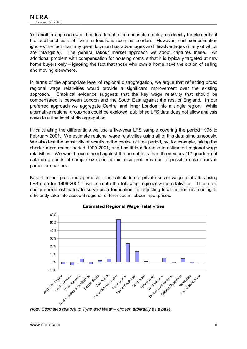
Based on our preferred approach – the calculation of private sector wage relativities using LFS data for 1996-2001 – we estimate the following regional wage relativities. These are our preferred estimates to serve as a foundation for adjusting local authorities funding to efficiently take into account regional differences in labour input prices.

Estimated Regional Wage Relativities

-10%

0%

10%

20%

30%

40%

50%

60%

Rest o

f Nort

h Eas

t

South

Yorksh

ire

Wes

t York

shire

Rest Y

orksh

ire & H

umbe

rside

East M

idlan

ds

East A

nglia

Centra

l & In

ner L

ondo

n

Outer L

ondo

n

Rest o

f Sou

th Eas

t

South

West

Tyne &

Wea

r

West M

idlan

ds

Rest o

f Wes

t Midl

ands

Greater

Man

ches

ter

Mersey

side

Rest o

f Nort

h Wes

t

Note: Estimated relative to Tyne and Wear – chosen arbitrarily as a base.

www.nera.com 1

1. INTRODUCTION

We were commissioned by the South East Area Cost Adjustment Group and Association of London Government to estimate regional wage differentials for England (using Labour Force Survey and New Earnings Survey data).

The context for the work is the question of how central government funding of local authorities should be adjusted to account for regional differences in labour costs to allow delivery of the same level of service in each region. Other funding adjustments, relating to local needs, are also made.

In section 2 we outline the context for the work, consider alternative approaches to calculating the ACA, and set out our broad approach to calculate regional wage relativities using labour market statistics.

In section 3 we calculate regional wage differentials using Labour Force Survey data.

In section 4 we calculate regional wage differentials using New Earnings Survey data.

In section 5 we set out the results of sensitivity analysis.

In section 6 we set out our conclusions.

Appendix A includes a detailed discussion of the statistical series used, while Appendix B includes the empirical results of our analysis. Appendices C to E provide additional supporting material.

www.nera.com 2

2. CONTEXT & METHODOLOGY

2.1. Summary

The context for our empirical analysis is the question of how to adjust central government funding for local authority services for differences in the price of labour inputs. A separate question is how funding should be adjusted to reflect the required volume of inputs. The intent of funding adjustments for relative input prices and volumes is to ensure that all local authorities have the same potential to deliver services of a given quality (for the same level of local council taxpayer input).

One approach suggested for adjusting local government funding - the “specific cost” approach - seeks to compensate local authorities directly for the additional costs they face. We reject the specific cost approach – as did the independent Elliot review of the area cost adjustment in its report of 1996 on grounds that the approach “fails to pass the tests of practicality, technical robustness, reliability of calculation and freedom from perverse incentives.”1

The approach we adopt to determining the relative adjustment for the labour cost component of local government activities is to examine regional wage differentials revealed by labour market statistics (the general labour market approach). We control statistically for factors such as education and occupation on wages to ensure a like-with-like comparison of locations (this turns out to reduce regional wage relativities). We consider private sector workers alone – since using existing public sector wage differentials to decide what public sector funding relativities ought to be would be circular and entirely uninformative.

2.2. The Underlying Problem

Local authorities in England receive central government funding for a range of services including, for example, police and education services. A key question is how to allocate overall funding to ensure that the cost to individual council taxpayers of funding authorities services to a notional common standard is the same across the country. This question can be considered in two parts:

• Differences in costs of producing a common level of service due to differences in the volume of inputs required to produce a given output, for example, due to differences in the number of school age children in each authority on education costs or differences in economic deprivation on police and welfare costs. We sometimes refer to this as needs.

• Differences in costs of producing a common level of service due to differences in the price of inputs required to produce a given output, for example, due to differences in labour costs for different authorities.

1 Elliott, R.F., McDonald, D., R. MacIver. July 1996. Review of the Area Cost Adjustment, Waverley Press, University of Aberdeen and the Department of Environment. Paragraph 5.5.4.

www.nera.com 3

The latter of these is referred to as the Area Cost Adjustment (ACA) component of the overall Standard Spending Assessment (SSA). The bulk of the ACA is related to direct and indirect labour costs. For example, the proportion of education costs currently attributed to direct and indirect labour costs is approximately 80 per cent.

The analysis in this report is directly relevant to the question of how to adjust relative funding for differences in the price of labour inputs (we do not address the wider questions of what overall level of funding is desirable, or how overall funding should be distributed between local authorities based on an assessment of relative needs and the relative price of inputs).

There is growing evidence that failure to adjust funding appropriately for regional wage relativities is causing problems in terms of equity and efficiency. For example, teacher vacancy rates are higher in London and the South East than in the rest of the country, while in the health sector some hospitals face severe funding constraints due to the need to use relatively expensive agency staff rather than pay the going rate for full time employees. There is also evidence that these problems are not just short-term recruitment problems – but long-term problems of recruitment and retention for workers across a range of experience levels.

2.3. Context & Alternative Approaches

The question of how to adjust central government funding of local authorities for differences in relative input prices is, not surprisingly, controversial amongst local authorities. In 1995 the Government commissioned an independent review of the ACA (we refer to the report as the “Elliot report”), and in July 1996 the review group reported recommending that regional pay premia should be identified using labour market statistics. Our approach is consistent with this recommendation. Alternative approaches have been suggested or applied elsewhere and we briefly comment on these.

The ACA is currently calculated based on relativities in average earnings between regions for occupational groups considered relevant to local government. New Earnings Survey (NES) data is used in the assessment. There are three problems with this approach:

• The NES excludes those who do not have a tax record (the low paid) – potentially biasing estimated relative wage differentials downwards (since the low paid will be relatively more numerous in areas with lower average pay).

• Using simple averages does not provide a like-with-like comparison since, for example, a worker in one location may be more highly qualified or experienced than a worker in the same occupation in another location.

• The approach is circular to the extent that the relativity for specific occupational groups such as teachers is used to decide what relative price adjustment for education funding ought to be. Such an approach would not resolve existing problems in recruiting and retaining teachers of appropriate skill in high relative wage locations, where jobs outside teaching (or teaching jobs in other regions) are particularly attractive, and it would introduce perverse incentives.

www.nera.com 4

National Health Service (NHS) funding is also adjusted for regional wage relativities according to the so-called Market Forces Factor (MFF).2 The MFF is based on analysis of NES data for private sector employees – controlling for factors such as age, sex, and industry occupation. The calculation is done separately for three years of data and then averaged for each zone.

The approach in the NHS therefore somewhat aims to ensure a like-with-like comparison, and to overcome circularity by calculating wage relativities for private sector workers. However, use of NES data does not allow characteristics such as employee qualifications to be controlled for, and is subject to the objection that the sample excludes the low paid. In addition, medical and dental staff are excluded from the application of the MFF and are instead subject to a “London Weighting” based on a pay index based on actual NHS trust pay data. The latter suffers from circularity.

An alternative to the current ACA that has been suggested would be to apply a so called specific cost approach similar in spirit to that applied for medical and dental staff in the NHS (or to apply a hybrid system with the specific cost approach applied to some employees). The approach seeks to compensate local authorities for the additional costs of attracting and retaining workers in high cost locations, including additional recruitment costs, and housing and other special allowances.

The 1996 Elliot report considered, and rejected, the specific cost approach noting that it “fails to pass the tests of practicality, technical robustness, reliability of calculation and freedom from perverse incentives.” The approach is complex, and basing future provision on past spend would introduce perverse incentives. In any case, private sector regional wage relativities calculated using a general labour market approach reflect (or compensate for) the underlying advantages and disadvantages to an employee of one location versus another (and it is reasonable to expect public sector workers to have similar preferences between locations based on factors such as the attractiveness of the environment and living costs).

Direct compensation for the additional costs of living in locations such as London has formed part of the response to recruitment and retention problems. For two reasons, we do not view cost compensation as a sound overall approach. First, cost compensation approaches implicitly assume that locations such as London only involve additional costs – ignoring attributes that many people find desirable. Second, in practice it is not possible to measure all the costs and benefits of each location, many of which are intangible.

Housing (and rental) costs do, however, provide a ‘sanity’ check on estimates of regional wage relativities since house prices both reflects regional pay relativities and are a large a component of the costs of living in different locations. Figure 2.1 shows the regional premium of standardised house prices relative to the North calculated by the Halifax (for

2 Department of Health. History of the Market Forces Factor. http://www.doh.gov.uk/pub/docs/doh/rawp1.pdf

www.nera.com 5

example, standardised house prices in the North were £61,782, while in London they were £179,558, a premium of almost 200 per cent).3

Figure 2.1 House Prices in England Compared to the North (Percentage premium)

0%

50%

100%

150%

200%

250%

Yorkshire &the Humber

North West EastMidlands

WestMidlands

East Anglia GreaterLondon

South West South East

Hou

se P

rices

Rel

ativ

e to

the

Nor

th

However, differences in house prices do not tell us what pay relativities for workers in different locations should be. Fortunately, as the Elliot enquiry noted, in the Wealth of Nations Adam Smith pointed out that labour market competition ensures “that the whole of the advantages and disadvantages of different employments of labour and stock must in the same neighbourhood be either perfectly equal or continually tending to equality” (Book 1, Chapter 10). Differences in regional wages, provided workers are compared on a like-for-like basis, reflect the relative net advantages of different locations.

Finally, “targeted” measures have from time to time been introduced to overcome recruitment problems in locations such as London – presumably in the belief that they are more cost effective than increasing pay. For example, funding of £250 million for the starter home initiative was spread over three years and targeted at key workers including nurses, teachers and police.4 A problem with this approach is that all groups of workers make location decisions taking account of factors such housing costs – not just the first-time buyers. Existing homeowners in London and the South East have the option of selling and moving to a lower cost location, while those renting face higher rental cost in high cost housing areas. Everyone in an area of expensive housing is affected - including owners who can sell and relocate, and those in rental accommodation. A forty-year old London local authority employee who needs a bigger house because of a growing family is, just as much as a first time buyer, affected by the cost of living in the area he or she lives in.

3 Halifax & Bank of Scotland plc. 11 January 2002. Halifax House Price Index – Fourth Quarter 2001. http://www.hbosplc.com/view/housepriceindex/housepriceindex.asp

4 DETR. 12 April 2001. Starter Home Initiative – Housing Factsheet No.6. The initiative is expected to help around 10,000 workers in total.

www.nera.com 6

2.4. Our Approach

Large firms know in spirit, if not in statistical detail, the way that pay varies widely across England. Housing costs are three-fold greater in Greater London compared to the North of England, while some areas have clean air and empty roads, and others are congested and polluted. Private sector employers learn what level of pay is required to attract and retain the required employees in each location - and to ensure that they are profitable.

In the public sector, however, these mechanisms do not function automatically. Decisions over funding, and to some extent pay, are taken centrally. An approach is required that enables wage relativities to be calculated and applied to public sector funding decisions.

For compositional reasons, the nature of the workforce differs from one part of the country to another. London has almost no shipbuilders; Wales has few stockbrokers. In calculating the labour component of the ACA, those variations must be built in. A representative worker, with comparable characteristics and qualifications, has to be studied in each region.

Our approach is to examine data on regional wage rates, and to apply statistical techniques to uncover the relativities due to location alone (ensuring a like-for-like comparison by controlling for other “explanatory variables” such as education, experience, occupation etc). For completeness, and to isolate the relative importance of different aspects of methodology, we use a range of data and techniques.

There is an economic reason why public funding should vary by area: public employers and private employers (and public employers in different regions) compete for talent. Illogically from an economist’s point of view, some still argue that a Swansea teacher should receive the same number of pound notes as a Guildford teacher. To ensure local authorities are able to deliver the desired level of quality, regional funding should reflect private sector wage relativities. Evidence supports the underlying economic logic. For example, levels of teacher pay have been shown empirically to be an important determinant of teacher recruitment and retention throughout a teaching career.5

In examining regional labour market pay differentials we examine both Labour Force Survey (LFS) and New Earnings Survey (NES) data (in Sections 3 and 4 respectively). The former includes the low paid and allows personal characteristics such as education to be controlled statistically, while the latter includes a larger sample and allows greater regional disaggregation using published data (the two statistical series are discussed in Appendix A).

We consider both public and private sector employees in our analysis – though argue that the only valid approach to establishing what public sector relativities ought to be is to look at private sector differentials. We also apply two different statistical techniques. One that compares the wages of workers in each region on a like-for-like basis, while the other examines changes in wages for those workers who move (the latter is the so called “fixed effects” method).

5 Peter Dolton and Wilbert van der Klaauw. March 1995. Leaving Teaching in the UK: A Duration Analysis. The Economic Journal, 105 (p431-444).

www.nera.com 7

In general we use a “panel” of five years of data for our analysis. This approach differs from analysing individual years and averaging the result (the current approach, for example, used to calculate the market forces factor for health). Our approach is preferred since the statistical inference about regional wage relativities draws on all the data simultaneously and a more robust conclusion can be reached.

In terms of geographical disaggregation we draw on data for England and Wales, and report results for 16 regions for England excluding the base category Tyne and Wear against which all relativities are calculated (note that the choice of base region is arbitrary). For London we disaggregate into three regions – central, inner and outer London. While alternative regional groupings could be explored we note that LFS data published by the Office of National Statistics does not allow analysis down to a fine level of dissagregation. A further breakdown to separate the city, for example, is performed using NES data.

An alternative to disaggregation as a way of addressing “cliff edges” is to consider aggregation across broader regions (excessive disaggregation will tend to shift or exacerbate, rather than resolve, “cliff edge” problems). Arguably the Inner and Central London labour markets are sufficiently closely integrated that a single wage relativity should apply to the combined region. We also estimate the relativity for this combined region using LFS data, and for Central, Inner and Outer London combined. The priority should be to reflect the large estimated wage relativities across broad regions in funding decisions. Boundary problems and the question of finer levels of disaggregation are second order in comparison.

www.nera.com 8

3. EMPIRICAL RESULTS – LABOUR FORCE SURVEY

3.1. Summary

The results in this section are based on analysis of Labour Force Survey (LFS) data (see Appendix A.1). These data cover the years 1996 to (the first part of) 2001. We apply a standard statistical technique to estimate regional wage relativities controlling for factors such as occupation and employee characteristics.

Figure 3.1 measures regional wage differentials.6 It does so in three ways. One shows the raw (or unadjusted) relativities for the private sector; one shows the estimated relativities for the public and private sectors combined; and one shows results for the private sector alone (the latter is our preferred approach). The unadjusted LFS data indicates very large regional wage relativities – in part to workforce and occupation differences between locations. Controlling for workplace and individual characteristics such as qualifications statistically we see that the estimated wage relativities are considerably reduced (this step is important and we note that controlling for qualifications is not possible using the alternative New Earnings Survey Data set). But they are still large for London and the South East, measured relative to Tyne and Wear.

Figure 3.1 Estimated Wage Relativities Using Labour Force Survey Data

-20%

0%

20%

40%

60%

80%

100%

120%

140%

160%

Rest o

f Nort

h Eas

t

South

Yorksh

ire

West Y

orksh

ire

Rest Y

orksh

ire & H

umbe

rside

East M

idlan

ds

East A

nglia

Centra

l Lon

don

Inner

Lond

on

Outer L

ondo

n

Rest o

f Sou

th Eas

t

South

West

Tyne &

Wea

r

West M

idlan

ds

Rest o

f Wes

t Midl

ands

Greater

Man

ches

ter

Mersey

side

Rest o

f Nort

h Wes

t

Wag

e R

elat

ivity

Private - Raw Data Public & Private - Regression esimates Private - Regression Estimates

6 The region used here is based upon where an individual works rather than where they live, to be consistent with the definition used in the New Earnings Survey which is based upon employer records and hence on where an individual works. Appendix D outlines how the various districts and counties are mapped into these regions.

www.nera.com 9

3.2. Public & Private Sector Weekly Wage

In Table B.1 in Appendix B the dependent variable (the variable we seek to explain) is the log of the weekly wage.7 Each column of Table B.1 is a separate wage equation describing the relationship between wages and other factors. (Table B.2 to Table B.8 also follow this format.)

Lots of factors, of course, affect how much people earn. By using regression equations, it is possible to calculate which of these influences really matter, and by how much. This is what a wage equation does: it allows for the possibility that a number of variables determine pay. In other words, each column in Table B.1 tells us how different factors influence wages in different regions of England and Wales. Tyne and Wear is treated as the base category against which others are compared. The choice of Tyne and Wear is arbitrary - some region has to be chosen as the reference case.

The numbers listed in the first column of Table B.1 reveal how the average level of pay in each region compares to the level in Tyne and Wear. For instance, in the first column of Table B.1 the Rest of North East has a “coefficient” of –0.057, corresponding to a percentage wage relativity of about 6 per cent.8

The first column of Table B.1 shows raw LFS averages for each region with no statistical adjustment. Large “coefficients” imply large differences in these averages relative to Tyne and Wear. For example, for Central, Inner and Outer London, the rest of the South East and West Midlands all differ from Tyne and Wear by more than ten per cent.

However, the first column of Table B.1 is not a good indicator of how earnings differ across England for a representative person. In reality the higher pay that the table shows for London is partly because, for example, there are barristers in the capital and very few elsewhere. The capital has more people in intrinsically high-paying kinds of occupations. What is needed, instead, is a standardized or like-for-like comparison. Box 3.1 illustrates how our preferred estimate is built up by controlling for successive factors such as age, education etc.

7 For technical reasons it is standard practice in this sort of analysis to work with the log of wages. 8 In Appendix B the numbers are “coefficients”. To convert these to percentages one must take their anti-log and

subtract one. There is also a number in brackets, which is a t-statistic. It reveals how statistically significant the wage difference is between the two regions. Numbers of 2 or more on t-statistics are generally taken to be statistically persuasive.

www.nera.com 10

Box 3.1 Illustration of successive steps taken to ensure a like-with-like comparison

• Column 1 in a table such as B1 is effectively just a simple average: the column takes everyone who works in an area and does not adjust for the fact that different places have different sorts of occupations or employees. It does not do a like-for-like comparison.

• Column 2 introduces three so-called personal controls. These are age, age squared, and gender.9 In this way, the equation factors out how old a person is and also whether a man or a woman. Column 2’s results looks similar to column 1.

• Column 3 brings into the equation a set of ethnic controls (in addition to the controls in Column 2). In other words, it allows for the possibility that people of different races and country backgrounds earn different amounts. This turns out not to produce important changes in the regional relativities.

• Column 4 introduces 40 qualification controls. This is important, because it is a way of adjusting for the differences by area in how many people have degrees, differences in their kinds of training, differences by region in levels of schooling, and so on. The relativities for Central London, Inner London and Outer London now drop significantly to 83 per cent, 42 per cent and 25 per cent respectively (from 116 per cent, 58 per cent and 31 per cent respectively). This step matters – we note that controlling for qualifications is not possible using the alternative New Earnings Survey Data set.

• Wages also depend on the industry in which someone works. Allowing for the industrial composition of a region makes a noticeable difference to our wage estimates. Adjustments are also made for the number of hours a person works and the length of their tenure in the job. Columns 5 & 6 explore the consequences of these changes. Central, Inner and Outer London wages are still significantly above wages elsewhere after we do a like-for-like comparison at 55 per cent, 34 per cent, and 21 per cent respectively. The overall impact of controlling statistically to ensure a like-for-like comparison has been to shrink the raw wage differentials.

Table B.1 takes a full random sample of all workers and therefore has both public-sector and private-sector employees. Intellectually, the problem with this is that the purpose of the analysis in this report, and more broadly in the whole ACA debate, is to decide how public sector funding regional allocations ought to be adjusted for labour input prices. Hence it is at best somewhat circular, and at worst potentially badly misleading, to base calculations on what a mixture of public and private people currently earn. We are trying to decide how things should - not do - operate. Private-sector regional wage differentials should therefore be the focus.

9 Including age squared is a standard approach, which, for technical reasons, allows the relationship between age and earnings over a working lifetime to be more accurately represented.

www.nera.com 11

3.3. Private Sector Weekly Wage

Table B.2 goes through the same steps as the table before it. The ‘raw’ wage relativities are now larger. By column 6 of Table B.2, the estimated regional dispersion of remuneration has shrunk again. There remains, even so, significantly higher pay in London especially.

The results so far have been for mean differences – with and without controlling for differences (OLS provides a mean estimate). However, means and therefore ordinary least squares are sensitive to outliers, and in the data there are a number of high outlier wage values.10 We want to ensure that our estimates are not heavily dependent on these.

A so-called median regression model provides one check on the influence of outliers, and this is estimated in column 7 of Table B.2 (we do not present median results anywhere else as they are computationally time consuming to estimate - column 7 needed nearly 2000 iterations to converge).11

The results in column 7 of Table B.2 are similar to those found in column 6 using OLS. This suggests that outliers are not unduly influencing the results. For example, that the results are not particularly sensitive to the inclusion of very highly paid individuals in London. As OLS is easier to compute, and the results are essentially the same, we concentrate on OLS estimates for the remainder of the report.

3.4. Public & Private Sector Hourly Wage

A potential objection to Table B.1 and Table B.2 is that the pay variable under scrutiny is not a per-hour rate.

Table B.3 remedies that by considering hourly pay obtained by dividing weekly earnings by the reported number of hours worked. The results do not, however, differ significantly between Table B.1 and

Table B.3.

3.5. Private Sector Hourly Wage

Table B.4 considers hourly wages for the private sector - much the same pattern is found as in Table B.2.

10 The mean and 99th percentiles of the LFS weekly wage across all regions are £298 and £1,174 respectively. The median is £250.

11 Statistically, the ‘median’ means half way up the distribution whereas the ‘mean’ is simply the average. The median regression finds the line that minimizes the sum of absolute residuals rather then the squares of the residuals as in OLS.

www.nera.com 12

4. EMPIRICAL RESULTS – NEW EARNINGS SURVEY

4.1. Summary

The New Earnings Survey Panel Data Set (NESPD, abbreviated to NES) is an annual survey of earnings based on individuals whose National Insurance numbers end in "14" (see Appendix A for further details). The data run from 1996 to 2000 inclusive and has the advantage that it is a larger sample than the LFS. However, the NES does not include the low paid (those not filing a tax return), or the qualifications for individuals in the sample. The former arguably biases estimated wage relativities downwards while the latter makes it difficult -- arguably impossible -- to do proper analysis of wage differentials because a like-for-like comparison cannot be achieved.

Figure 4.1 shows the raw (unadjusted) average relativities for the NES, and the estimated relativities for the public and private sectors combined, and the private sector alone using OLS. The spread of relativities is smaller than found using the LFS, and the differential between public and private, and private sector only results is also small. However, the broad patterns are very similar to those found using LFS data.

Figure 4.1 Estimated Wage Relativities Using New Earnings Survey Data

-20%

0%

20%

40%

60%

80%

100%

Rest o

f Nort

h Eas

t

South

Yorksh

ire

West Y

orksh

ire

Rest Y

orksh

ire & H

umbe

rside

East M

idlan

ds

East A

nglia

Centra

l Lon

don

Inner

Lond

on

Outer L

ondo

n

Rest o

f Sou

th Eas

t

South

West

Tyne &

Wea

r

West M

idlan

ds

Rest o

f Wes

t Midl

ands

Greater

Man

ches

ter

Mersey

side

Rest o

f Nort

h Wes

t

Wag

e R

elat

ivity

Private - Raw Data Public & Private - Regression Estimates Private - Regression Estimates

www.nera.com 13

4.2. Public & Private Sector

Table B.5 for the NES builds up to a full specification, column by column, in a way that is designed to follow the spirit of Table B.1 for the Labour Force Survey (though it is not possible with the NES to include employee qualifications).12 When occupation variables are added in column 6 there is a marked drop in the regional spread of pay (seventy-one occupations are included in the wage equation).

4.3. Private Sector

Table B.6 uses the private sector sample of employees from the New Earnings Survey. When an allowance is made for occupation the Central London relativity diminishes to 41 per cent (column 6).

4.4. Public & Private Sector Using Fixed Effect Method

A feature of NES data is that people are followed through time; the same individuals can then be studied one year after another. This has strengths and weaknesses. First, it is an advantage in principle, because it allows the unchanging characteristics of people (their drive, genes, personality, and so on) to be ‘differenced out’. Second, it has the disadvantage that all the regional information is then only coming from those who move from one area to another.

12 The definition of the private sector in the NES is complicated by the fact that the public sector variable included in the dataset in all the years prior to 1998 was not provided for the years 1999 or 2000. To achieve consistency, a public sector variable was created using information for 1998. The main public sector occupations were identified and then mapped into 1999 and 2000. This variable is used to derive a private sector sub-sample in Table B.6 and columns 1-3 and 5 of Table B.8. An alternative public sector variable was derived by Wilson et al (2001) and is used in columns 4&6 of Table B.8. This variable is derived using a matching algorithm that uses both industry and occupation. The main difference between the two definitions of the public sector is that the Warwick variable includes workers who work in both the public and the private sectors such as secretaries and clerks. The variable we use is based on occupations primarily confined to the public sector such as police, firemen, prison officers etc.

www.nera.com 14

Table B.7 is a wage equation estimated using ‘fixed effect’ methods. This means that everything fixed about people is allowed for, from one period to the next, when calculating how wages vary. Intuitively, this is achieved by looking at how a worker’s wage changes when he or she switches from one part of the country to another. In theory, that makes possible a more efficient estimate of the other forces that mould pay. Unfortunately, however, the possibility of measurement error in the NESPD – where individuals are wrongly classified in some way - means that the supposed superiority of the fixed effects estimator cannot be taken for granted. The consequences of such measurement error would be to bias downwards the size of any estimated wage relativity (see Appendix E).

In column 1 of

www.nera.com 15

Table B.7, Central London’s wage relativity is 19.7 per cent – significantly lower than the raw differentials in Table B.1 to Table B.6. The picture painted by NES fixed effects estimation is of a country with only a slender amount of wage dispersion across different areas. Such a view contrasts dramatically with most of the earlier tables in this report.

4.5. Private Sector Using Fixed Effects

Table B.8 uses a private sector only sample for fixed-effects estimation. The conclusion is that, in comparison to Tyne and Wear, wages are about 15 per cent higher in Central London, 11 per cent higher in Inner London, 5 per cent higher in Outer London, 3 per cent higher in the Rest of the South East, and 3 per cent higher in the West Midlands. Everywhere else is similar to the Tyne and Wear pay level, with West Yorkshire the lowest area in the country, where wages are estimated to be 4 per cent lower than in Tyne and Wear. Results are similar using both definitions of the private sector – see for example columns 5 and 6 of Table B.8. Controlling for industry and occupation makes little difference.

4.6. Further Analysis of Movers

Fixed-effects analysis has shrunk the wage relativities dramatically compared with OLS estimates. To get to the bottom of the cause of these smaller wage differentials, it is of interest to look more closely at the individuals in our data who are moving regions.

Once that is done, there is good reason to be sceptical of the representativeness of the NES when it comes to the characteristics of those individuals who move locations – the so-called switchers. The fact that, as we noted above, recent regional migrants are excluded from the sample compounds a further difficulty, namely, that the sample of switchers is quite different from those who do not move – the ‘stayers’. Also, there are relatively few switchers.

In total, from 99579 people on whom we have wage data in 1999 and 2000, only 6.3 per cent moved within the region where they worked. Note that this is many more than if we used region of residence - mostly because of moves inside the South East. On average, the stayers made £329 per week in 1999 and £349 in 2000, compared with £366 and £403 for the movers.

Out of 5275 people working in Central London in 1999, 4720 of them were also working there in 2000 (94 per cent of the total). Of the 555 who moved from Central London, their 1999 salary levels and change-in-salary from 1999-2000 are given in the first four rows of Table 4.1, where the figure in parentheses is the change that year. The following rows show the changes in income for moves within London, and for moves to London from elsewhere.

www.nera.com 16

Table 4.1 Income Changes for those Moving to and from London

Moving from Moving to Number of

movers

Weekly income & change (in brackets)

Relative change

From Central London

Central London Inner London 91 £438 (£59) 13% Central London Outer London 171 £403 (£4) 1% Central London Reset of SE 160 £467 (£40) 9% Central London Rest of E&W 133 £517 (-£8) -2% Within London & SE

Inner London Central London 156 £448 (£36) 8% Outer London Central London 140 £409 (£74) 18% Rest of SE Central London 145 £412 (£91) 22% From Rest of E&W to London & SE

Rest of E&W Central London 186 £341 (£145) 43% Rest of E&W Inner London 31 £396 (£127) 35% Rest of E&W Outer London 145 £312 (£28) 9% Rest of E&W Rest of SE 517 £368 (£48) 13% Note: SE refers to South East and E&W refers to England and Wales.

The movers out of Central London to the rest of England and Wales thus appear to be very special since their income does not fall significantly (-2 per cent). We believe that this helps explain the lower regional wage estimates that come out of a fixed-effects approach. In contrast, the movers to central, inner and outer London from the rest of England and Wales gain significant increases in pay – broadly consistent with the results of cross section analysis of stayers.

Our judgement is that this is because, even when they are moving to cheap areas, human beings find it very difficult to take nominal wage cuts. To persuade a manager to leave London to run her Newcastle branch, it is likely that the firm has to pay above the odds for the region into which she is being sent. But if that is so, it is not sensible to calculate regional pay differentials by looking at the switchers. Those who stay in an area dominantly determine, and become acclimatised to, the going rate of pay. The stayers are the ones who matter. Looking at switchers can be highly misleading.

www.nera.com 17

5. SENSITIVITY ANALYSIS

5.1. Summary

In this section we consider various sub-samples of the population to test the sensitivity of the results. In addition, we explore the impact of the choice of time period for analysis and the choice of level of regional aggregation (within London) on the results.

We find that calculated regional wage relativities are relatively insensitive to various divisions of the sample population, for example, into males and females, those over and under 30 years of age, those without qualifications and those with higher degrees, broad occupational groupings and the choice of time period (or sub-period). The results differ – but not by much – supporting a conclusion that our analysis has uncovered robust like-with-like regional wage relativities.

Tables B.9 and B.10 show the results for the LFS by broad occupational grouping and for two different time periods. Tables B.11a and B.11b provide a number of additional disaggregations for the LFS and NES data sets respectively.

5.2. Sensitivity to Occupational Grouping

Because the Labour Force Survey is a random sample of the whole working population, it can be used to create sub-samples of any sort that is required. Table B.9 shows how pay differs by area for particular groups of workers.

Figure 5.1 shows the results for the public and private sectors (Column 6 of Table B.9). For London and the South East the broad patterns for each occupational group are the similar – in particular, the estimated wage relativities for managers and professionals and manual workers are very close. This implies a degree of robustness to the estimated wage differentials using all occupational groups together – which suggests that attempting to isolate occupational groups “similar” to local authority employees is unlikely to be productive (and would reduce both the simplicity of the approach and sample size and statistical robustness). It also suggests that wage differentials approximate a percentage differential across a range of incomes – rather than a fixed absolute difference in pay by location irrespective of income.

www.nera.com 18

Figure 5.1 Estimated Regional Wage Relativities by Occupational Group

-20%

-10%

0%

10%

20%

30%

40%

50%

60%

70%

Rest o

f Nort

h Eas

t

South

Yorksh

ire

Wes

t York

shire

Rest Y

orksh

ire &

Hum

bersi

de

East M

idlan

ds

East A

nglia

Centra

l Lon

don

Inner

Lond

on

Outer L

ondo

n

Rest o

f Sou

th Eas

t

South

West

Tyne &

Wea

r

West M

idlan

ds

Rest o

f Wes

t Midl

ands

Greater

Man

ches

ter

Mersey

side

Rest o

f Nort

h Wes

t

Wag

e R

elat

ivity

Managers & Professionals Non-manuals - technical Manual workers

5.3. Sensitivity to Time Period

Figure 5.2 shows results for the LFS public and private sector data for the periods 1993-95 Table B.10) and 1996-2001 (Table B.1).

Figure 5.2 Estimated Regional Wage Relativity by Time Period

-10%

0%

10%

20%

30%

40%

50%

60%

Rest o

f Nort

h Eas

t

South

Yorksh

ire

West Y

orksh

ire

Rest Y

orksh

ire & H

umbe

rside

East M

idlan

ds

East A

nglia

Centra

l Lon

don

Inner

Lond

on

Outer L

ondo

n

Rest o

f Sou

th Eas

t

South

West

Tynne

& Wea

r

West M

idlan

ds

Rest o

f Wes

t Midl

ands

Greater

Man

ches

ter

Mersey

side

Rest o

f Nort

h Wes

t

Wag

e R

elat

ivity

1993-95 1996-01

www.nera.com 19

Figure 5.2 suggests that even though real incomes have grown relatively faster in the South East, that some of this growth may be due to compositional changes in the workforce, since our calculated relativities allowing for such changes are very similar between the periods.

5.4. Sensitivity to Level of Regional Aggregation

Table B.11A includes estimates for London aggregated into Central and Inner London, and Central, Inner and Outer London. The private sector relativity for Central and Inner London combined is 53.9 per cent, versus 65.5 per cent and 37.8 per cent respectively considered separately. There is a case for considering Central and Inner London as a single region given their closely integrated labour markets. We also examine the sensitivity of results to inclusion/exclusion of the City of London in Table B.11B (this is not possible with published LFS data). We find that excluding the City reduces the relativity for Inner London from 38.1 to 34.0 per cent, while with Central and Inner London merged we see a reduction from 34.0 to 31.0 per cent. We do not consider that there are grounds for excluding the City of London.

5.5. Further Sensitivity Analysis

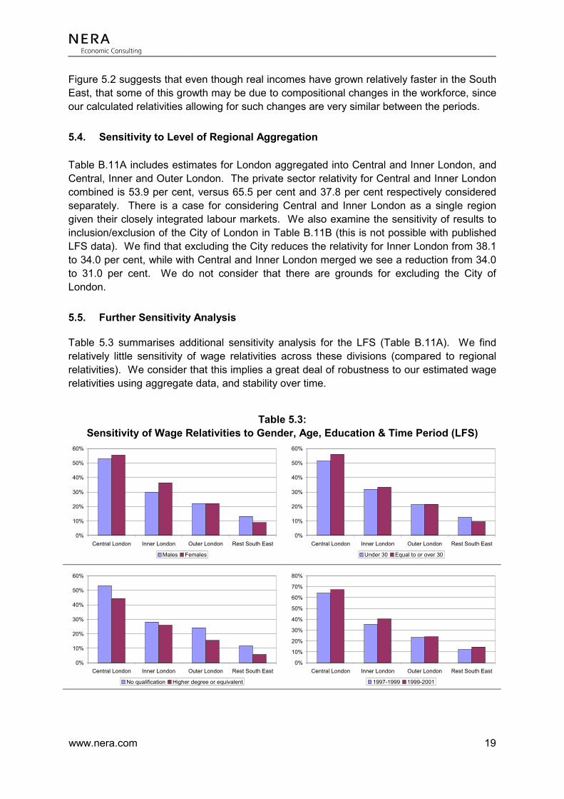
Table 5.3 summarises additional sensitivity analysis for the LFS (Table B.11A). We find relatively little sensitivity of wage relativities across these divisions (compared to regional relativities). We consider that this implies a great deal of robustness to our estimated wage relativities using aggregate data, and stability over time.

Table 5.3: Sensitivity of Wage Relativities to Gender, Age, Education & Time Period (LFS)

0%

10%

20%

30%

40%

50%

60%

Central London Inner London Outer London Rest South East

Males Females

0%

10%

20%

30%

40%

50%

60%


Under 30 Equal to or over 30

0%

10%

20%

30%

40%

50%

60%


No qualification Higher degree or equivalent

0%

10%

20%

30%

40%

50%

60%

70%

80%


1997-1999 1999-2001

www.nera.com 20

6. CONCLUSIONS

We conclude that the best approach to calculating regional wage relativities is to calculate them using the Labour Force Survey (LFS). This data source includes the low paid and allows us to do proper like-for-like comparisons of workers across areas (for example, by allowing for the effect of educational qualifications on wages).

We focus on private sector employees since regional wage relativities for these workers reflect the underlying advantages and disadvantages of each region. We use standard statistical techniques to calculate our estimates using a five-year sample of LFS data covering the period 1996-2001. The results are shown in Table 6.1. These are our preferred estimates and serve as a basis for adjusting central government funding for local authorities to take account of differences in labour input prices. Our conclusions are similar to those reached by Professor Elliott’s independent inquiry.

Table 6.1 Estimated Regional Wage Relativities

(Using private sector LFS data for 1996-2001)

Region Wage Relativity

Central & Inner London 53.9% Outer London 23.6% Rest of South East 13.2% West Midlands 5.0% Greater Manchester 4.5% West Yorkshire 4.3% East Anglia 3.5% Rest of North East 2.2% East Midlands 1.8% South West 0.9% Tyne and Wear 0% Rest of North West -0.1% Rest of West Midlands -0.8% Merseyside -1.4% Rest of Yorkshire and Humberside -2.7% South Yorkshire -3.6%

Note: All estimates are relative to Tyne and Wear Source: NERA calculations (see Appendix B, Table B.2 column 6), and Table B.11A.

www.nera.com 21

APPENDIX A. THE DATA SETS

A.1. Labour Force Survey

The Labour Force Survey (LFS) is a survey of households living at private addresses in Great Britain. Its purpose is to provide information about the UK labour market that can be used to develop, manage, evaluate and report on labour market policies. It is carried out by the Social Survey Division (SSD) of the Office for National Statistics (ONS) in Great Britain, and by the Central Survey Unit of the Department of Finance and Personnel in Northern Ireland on behalf of the Department of Economic Development. The first LFS in the UK was conducted in 1973, under a Regulation derived from the Treaty of Rome. The Statistical Office of the European Union (Eurostat) co-ordinates information from labour force surveys in the member states in order to assist the EC in matters such as the allocation of the European Social Fund.

The ONS is responsible for delivering UK data to Eurostat. The survey was carried out every two years from 1973 to 1983 in the spring quarter and was used increasingly by UK Government departments to obtain information that could assist in the framing and monitoring of social and economic policy. By 1983 it was being used by the Employment Department to obtain measures of unemployment (on a different basis from the monthly claimant count) and to obtain information that was not available from other sources or was only available for census years. For example, the surveys can give estimates of the number of people self-employed. Other than the Census, the LFS is the only really comprehensive source of information about the labour market. Between 1984 and 1991, the survey was carried out annually and consisted of two elements:

• A quarterly survey of approximately 15,000 private households, conducted in Great Britain throughout the year;

• A "boost" survey in the quarter between March and May, of over 44,000 private households in Great Britain and 5,200 households in Northern Ireland.

Published estimates for 1984-1991 are available for the UK and are based on the combined data from the "boost" surveys and quarterly surveys in the spring quarters (Mar-May).

Since Spring 1992, LFS refers to the seasonal quarters March-May (Spring), June-August (Summer), September-November (Autumn) and December-February (Winter). LFS microdata are available in databases covering these periods.

Whilst questions in the LFS are continually being added, removed or modified, the major change to the quarterly survey was the introduction of a section of income questions from winter 1992/93 onwards. These questions were only asked of respondents receiving their fifth and final interviews, because of concerns that the questions might have an adverse impact on overall response rates. The LFS is an important source of income data, particularly for part-time workers. However, because income questions were initially only asked in wave-5 interviews, sample sizes were quite small and the associated sampling errors tended to be relatively big. Work was done to test whether asking income questions in

www.nera.com 22

the first wave would lead to higher non-response in later waves, as was believed would be the case, but no evidence was found to support that belief. So, from Spring 1997, income questions were asked in both waves 1 and 5. This doubled the sample size and reduced sampling errors by about 30 per cent.

Each quarter's LFS sample of 61,000 UK households is made up of five "waves". Each wave is interviewed in five successive quarters, such that in any one quarter, one wave will be receiving their first interview, one wave their second, and so on, with one wave receiving their fifth and final interview. Thus there is an 80 per cent overlap in the samples for each successive quarter. Households are interviewed face to face at their first inclusion in the survey and by telephone, if possible, at quarterly intervals thereafter, and have their fifth and last quarterly interview on the anniversary of the first.

The survey results refer to persons resident in private households and in NHS accommodation in the UK. For most people, residence at an address is unambiguous. Individuals with more than one address are counted as resident at the sample address if they regard that as their main residence. The following are also counted as being resident at an address:

• people who normally live there, but are on holiday, away on business, or in hospital, unless they have been living away from the address for six months or more;

• children aged 16 and under, even if they are at boarding or other schools;

• students aged 16 and over are counted as resident at their normal term-time address even if it is vacation time and they may be away from it.

For further details of sample design and methodology, see the Labour Force Survey User Guide Volume 1: Background & Methodology, February 2001.

A.2. New Earnings Survey

The New Earnings Survey Panel Data Set (NESPD) is an annual survey of earnings collected under the Statistics of Trade Act 1967. The NES is sampled on individuals whose National Insurance numbers end in "14". Since the same pair of terminating digits are used as the basis for each year's sample, a longitudinal panel is automatically generated within the Surveys. Since a National Insurance number is issued to each individual on attaining the minimum school-leaving age, the sample frame implies that, conditional on a balanced response rate, the Survey represents a random sample of all employees in employment, irrespective of employment status, occupation, size or type of employer, or type of job. The survey reference date is usually the 2nd Thursday in April. There is no grossing, weighting or imputation undertaken for non-response or sample frame deficiencies. Certain categories of employees are not selected: for example the Armed Forces, those employed in Enterprise Zones, those in private domestic service, occupational pensioners, non-salaried directors, those employed outside Great Britain, persons working for their spouses and clergymen holding pastoral appointments.

www.nera.com 23

The legal obligation on employers to complete the Survey questionnaire, and its basis in the employer's payroll records, ensure both a high response rate and a high degree of accuracy in the earnings information. Moreover, should an individual not be included in the NES in any year, due for example to unemployment, temporary withdrawal from the labour force, or a failure of sample location, the sampling frame ensures that he should be located for the Survey in any future year when he is in employment. Consequently, absence from the sample frame or failures of sample location do not lead to cumulative attrition. Such a sample frame implies that, conditional on a 100 per cent response rate, NESPD is a one percent sample of employees in employment.

As with most surveys, however, NESPD does not capture everyone in the sample frame even though there is a legal obligation to try to do so. The main problem arises in the way in which the survey is carried out. Questionnaires are sent to employers for completion; the required addresses are taken from a database at the tax office. This is the most accurate way of obtaining these addresses although it is also a major source of under sampling because there are many employees without a current tax record. Thus new firms as well as small firms are under-represented in the database, which will also inevitably be out-of-date when the sample is taken.

There are two main reasons for an individual not having a current tax record. First, the individual may have recently changed jobs and therefore not have a current record at that point. Or, second, he/she may not earn enough to pay tax or national insurance. In either case the individual is not covered in the NESPD sample, although they may be in the NESPD sample frame.

A.3. Implications of Underlying Income Distribution

Table A.1 explores the implications of the sample of workers in the NES more deeply. Consider the pay distributions set out in the upper half of Table A.1. These describe the patterns across different wage bands within the economy. People are divided into so-called percentiles. These are cut-off levels. The 1-percentile group means those in the bottom one percent of all earners in England: these are the very low paid. The 99-percentile means the opposite: this is the cut-off that measures the highest one percent of earners in the economy. The 50 percentile means those people who are exactly average. To be precise, if a statistician finds that Mr X is the 87th percentile person in the wage distribution, that means there are 13 per cent of people who earn more than Mr X, and 87 per cent of people who earn less than or equal to Mr X.

The top left-hand number in Table A.1, for instance, is £2.3. This implies that if we look at people in the bottom one percent of the pay distribution, the average hourly wage among the worst paid is £2.30 per hour. If they earned a little more, they would push up out of the bottom 1-percentile group.

In the first column of the pay figures in Table A.1, the hourly wage level - moving steadily up the percentiles - goes from £3.90 an hour for the 10th percentile worker, to £7.10 for the 50th percentile worker, to £15.40 for the 90th percentile worker.

www.nera.com 24

As can be seen from the upper half of Table A.1, in Central London there is a much greater wage among the high-paid group than is found elsewhere in the country. This is just an alternative way to express the regional wage premia estimated earlier in this report. To be in the top 1 per cent of earners in Central London, you have to earn at least £60.80 an hour. To be in the top one percent in the Rest of the South East, where people are better paid than in most of the country, you have to earn at least £26.80 per hour. In the lower half of Table A.1, for LFS rather than NES data, the same general pattern is found.

One striking difference emerges, however, between the New Earnings Survey and Labour Force Survey numbers. Table A.1 reveals that the average wage in 1996-2000 in NES was £8.96 per hour. By contrast, the average hourly wage according to the LFS data in Table A.1 was, in 1996 to 2000, £8.18 an hour. Thus NES tells us that average pay in the country is ten percent greater than recorded in LFS. This is a serious discrepancy between the two data sets.

We believe it is clear, from our examination of the data, what is going on. The New Earnings Survey is misleading as a source of pay information in England and Wales: it is the bottom end of the wage distribution, not the top end, where NES goes wrong. In Central London, according to Table A.1, the average wage is £14.55 in NES data and £14.70 in LFS data. For most purposes, these two numbers can be viewed as (satisfactorily) identical. That is not true lower down. For example, in the Rest of the England and Wales, the average wage is £8.12 per hour in NES data and £7.40 per hour in LFS data – another ten percent divergence.

What is causing the apparent sampling problem with NES?

• First, the New Earnings Survey omits people who do not file a tax return. Under the British system, then, this is a powerful bias towards the sampling of well-off workers and against the sampling of poorly paid people. The low-paid are dramatically under-represented in NES.

• Second, it is not merely that the New Earnings Survey fails to count a tranche of the country’s poorest people. Because taxpayers are not spread evenly across the country, this leads to an important regional distortion. Tax levels apply nationally: whether you live in Guildford or Greenock you face the same tax bands on your income. But in London, where average wages are high, it is rare for a worker to be a non-taxpayer. Outside the South East, it is more common. This means that the slice of omitted low-paid people in NES data differs a great deal in size from one part of the country. The omission of individuals comes with a price. Biases are produced.

• Third, NES excludes people who have recently moved region. This may not be a problem for some purposes, but is potentially a serious difficulty if the aim is to understand the wages of inter-regional migrants (which is effectively what a fixed effects analysis relies on).

www.nera.com 25

Table A.1 Hourly wage distributions (£)

Percentiles All Central London

Inner London Outer London Rest SE Rest England & Wales

NES 1996-2000 1 2.3 3.0 2.5 2.5 2.3 2.2 5 3.5 4.6 4.0 3.8 3.6 3.4 10 3.9 5.6 4.8 4.3 4.1 3.8 25 5.1 7.9 6.4 5.4 5.3 4.8 50 7.1 11.3 9.0 7.8 7.4 6.7 75 10.6 16.8 13.2 11.7 11.1 9.7 90 15.4 26.2 18.8 16.7 16.2 14.0 95 19.2 35.1 24.2 20.7 20.3 17.2 99 32.4 60.8 44.9 32.9 32.9 26.8 Mean 8.96 14.55 11.18 9.60 9.23 8.12 Percentiles All Central

London Inner London Outer London Rest SE Rest England

& Wales LFS 1996-2001 1 1.5 2.6 1.7 1.8 1.6 1.5 5 2.9 4.5 3.5 3.2 3 2.8 10 3.5 5.7 4.3 3.9 3.6 3.3 25 4.6 8.2 6.1 5.3 4.8 4.3 50 6.6 11.7 9.2 7.7 6.9 6.1 75 10.0 17.7 13.0 11.5 10.4 9.1 90 14.4 26.1 18.5 16.0 15.2 12.9 95 18.0 33.7 23.1 20.0 19.1 15.7 99 30.0 52.9 38.5 33.7 30.8 24.2 Mean 8.18 14.70 10.79 9.45 8.52 7.40 Difference in mean wage

NES less LFS 0.78 -0.15 0.39 0.15 0.71 0.72

www.nera.com 26

APPENDIX B. EMPIRICAL RESULTS Table B.1

Log weekly wage – public & private sectors (LFS)

1 2 3 4 5 6 Rest of North East -.057 (3.95) -.052 (4.26) -.052 (4.29) -.046 (4.10) -.028 (3.51) -.025 (3.12) South Yorkshire -.054 (3.40) -.043 (3.21) -.041 (3.09) -.037 (2.98) -.033 (3.74) -.027 (3.05) West Yorkshire .030 (2.17) .052 (4.39) .059 (5.03) .041 (3.76) .029 (3.71) .031 (4.00) Rest Yorks & Humberside -.066 (4.50) -.056 (4.45) -.056 (4.48) -.056 (4.81) -.039 (4.80) -.036 (4.38) East Midlands -.013 (1.04) -.000 (0.01) .002 (0.21) .010 (0.99) .001 (0.14) .006 (0.84) East Anglia .022 (1.60) .035 (2.98) .035 (3.02) .025 (2.33) .020 (2.59) .017 (2.15) Central London .819 (58.03) .745 (62.11) .769 (63.90) .605 (53.86) .438 (54.35) .438 (55.03) Inner London .452 (30.43) .421 (33.33) .459 (36.06) .353 (29.83) .279 (33.07) .289 (34.74) Outer London .226 (17.01) .245 (21.69) .268 (23.63) .221 (20.91) .198 (26.42) .193 (26.09) Rest of South East .118 (9.91) .146 (14.41) .149 (14.70) .111 (11.78) .099 (14.77) .095 (14.33) South West -.018 (1.50) .005 (0.54) .006 (0.57) -.024 (2.46) -.004 (0.59) -.005 (0.72) West Midlands .101 (7.49) .090 (7.82) .103 (8.98) .096 (8.96) .044 (5.80) .041 (5.48) Rest of West Midlands -.043 (3.21) -.015 (1.30) -.013 (1.19) -.011 (1.00) -.023 (2.96) -.021 (2.74) Greater Manchester .074 (5.35) .085 (7.19) .089 (7.60) .064 (5.83) .031 (3.98) .031 (4.09) Merseyside .002 (0.15) .024 (1.75) .024 (1.74) -.005 (0.37) -.001 (0.19) .000 (0.02) Rest of North West .027 (1.96) .032 (2.72) .032 (2.78) .011 (1.01) -.007 (0.87) -.010 (1.29) Wales -.021 (1.55) -.009 (0.78) -.009 (0.81) -.014 (1.31) -.028 (3.65) -.024 (3.14) Personal controls (3) No Yes Yes Yes Yes Yes Ethnic controls (8) No No Yes Yes Yes Yes Qualifications (40) No No No Yes Yes Yes Work controls (2) No No No No Yes Yes 1 digit industry (11) No No No No Yes No 2 digit industry (60) No No No No No Yes Adjusted R2 .0476 .3119 .3148 .4111 .7017 .7112 N 264314 264314 264281 264160 262713 262713 F 601.8 4792.7 3281.8 2997.3 6526.4 5913.8 Notes:

Estimates are all in relation to the excluded category of Tyne & Wear.

Source: Labour Force Surveys, 1996-2001. All equations also include 5 year dummies. 1. Column 1 is the simplest calculation. It ignores all the factors that mould pay except for one, namely, the

region. These, therefore, are raw wage differentials area-by-area.

2. Column 2 assumes that two other things influence pay. One is a person’s age and the other is their gender. Thus the numbers next to the region names in Column 2 measure how pay varies across these areas after we factor out (or ‘hold constant’ in the jargon) age and gender.

3. Column 3 extends this list of possible influences to include ethnic background. It factors out from the wage equation a set of nine measures for a person’s race and four measures of where they were born.

4. Column 4 allows for a long set of (forty) different levels of qualification, as well as all the earlier factors. This is a particularly important step in providing a correct comparison of people between one region and another.

5. Column 5 allows for the number of hours the employee spends working, and the length of the person’s job tenure in the workplace. It also allows for which industry the person is employed in (grouping the country into approximately a dozen industries).

6. Column 6 adjusts for the number of hours the employee spends working, and the length of the person’s job tenure in the workplace. It also allows for which industry the person is employed within (grouping the country into approximately sixty different industries).

www.nera.com 27

Table B.2 Log weekly wage – private sectors (LFS)

1 2 3 4 5 6 7 Rest of North East -.045 (2.56) -.043 (2.98) -.044 (3.04) -.032 (2.34) -.034 (2.62) -.022 (2.27) -.014 (1.49) South Yorkshire -.054 (2.76) -.054 (3.35) -.053 (3.29) -.034 (2.24) -.039 (2.73) -.037 (3.46) -.029 (2.78) West Yorkshire .067 (3.91) .085 (6.00) .095 (6.77) .082 (6.12) .069 (5.44) .042 (4.42) .039 (4.27) Rest Yorks Humberside -.058 (3.19) -.045 (3.04) -.045 (3.06) -.041 (2.94) -.026 (1.95) -.027 (2.76) -.023 (2.43) East Midlands .022 (1.37) .036 (2.73) .040 (3.05) .050 (4.08) .045 (3.84) .018 (2.09) .016 (1.93) East Anglia .049 (2.89) .066 (4.69) .067 (4.80) .059 (4.51) .071 (5.62) .034 (3.63) .043 (4.81) Central London .904

(53.19) .837

(59.69) .873

(62.10) .684

(51.28) .634

(49.46) .504

(52.46) .486 (52.7)

Inner London .483 (26.01)

.450 (29.33)

.506 (32.79)

.397 (27.24)

.421 (30.31)

.319 (30.64)

.324 (32.4)

Outer London .269 (16.50)

.286 (21.26)

.323 (23.91)

.270 (21.19)

.280 (23.06)

.211 (23.24)

.218 (24.9)

Rest of South East .166 (11.27)

.200 (16.42)

.205 (16.90)

.161 (14.08)

.169 (15.56)

.124 (15.24)

.124 (15.9)

South West -.010 (0.65) .028 (2.19) .029 (2.30) .004 (0.30) .018 (1.57) .009 (1.01) .019 (2.28) West Midlands .143 (8.67) .117 (8.59) .136 (9.98) .136

(10.62) .102 (8.29) .049 (5.31) .053 (5.99)

Rest of West Midlands -.012 (0.75) .015 (1.13) .018 (1.35) .025 (1.91) .023 (1.92) -.008 (0.90) -.006 (0.71) Greater Manchester .094 (5.49) .104 (7.40) .111 (7.92) .091 (6.90) .083 (6.62) .044 (4.66) .036 (4.02) Merseyside -.034 (1.65) -.001 (0.05) -.001 (0.08) -.011 (0.70) .009 (0.62) -.014 (1.28) .007 (0.68) Rest of North West .057 (3.35) .060 (4.26) .061 (4.40) .038 (2.90) .030 (2.38) -.001 (0.16) .010 (1.13) Wales -.020 (1.16) -.005 (0.42) -.005 (0.38) .005 (0.35) .003 (0.23) -.027 (2.89) -.017 (1.87) Median regression No No No No No No Yes Personal controls No Yes Yes Yes Yes Yes Yes Ethnic controls No No Yes Yes Yes Yes Yes Qualifications No No No Yes Yes Yes Yes Work controls No No No No Yes Yes Yes 2 digit industry No No No No No Yes Yes Adjusted R2/ Pseudo R2 .0551 .3565 .3611 .4329 .4872 .7057 .5007 N 191997 191997 191979 191880 191828 190917 190917 F 510.0 4254.9 2931.7 1903.6 1441.0 4223.3 Notes:



region. These, therefore, are raw wage differentials area-by-area. They do not do a like-for-like comparison.



4. Column 4 allows for a long set of (forty) different levels of qualification, as well as all the earlier factors. This is a particularly important step in allowing a correct comparison of people between one region and another.


6. Column 6 allows for the number of hours the employee spends working, and the length of the person’s job tenure in the workplace. It also allows for which industry the person is employed within (grouping the country into approximately sixty different industries).

7. Column 7 uses median regression methods. The median regression finds the line that minimizes the sum of absolute residuals rather then the squares of the residuals as in Ordinary Least Squares, which we use to derive the other results.

www.nera.com 28

Table B.3 Log hourly wage – public & private sectors (LFS)

1 2 3 4 5 6 Rest of North East -.019 (2.00) -.020 (2.24) -.020 (2.28) -.013 (1.72) -.013 (1.74) -.011 (1.48) South Yorkshire -.024 (2.25) -.020 (2.09) -.018 (1.93) -.016 (1.90) -.017 (2.11) -.011 (1.33) West Yorkshire .034 (3.66) .047 (5.52) .053 (6.28) .030 (4.03) .035 (4.88) .036 (5.08) Rest Yorks Humberside -.037 (3.70) -.032 (3.61) -.033 (3.63) -.024 (3.10) -.019 (2.48) -.017 (2.31) East Midlands -.003 (0.38) .003 (0.34) .006 (0.72) .010 (1.51) .019 (2.90) .023 (3.50) East Anglia .036 (3.92) .042 (4.95) .043 (5.11) .036 (4.86) .046 (6.47) .041 (5.81) Central London .661 (70.38) .634 (74.10) .660 (76.82) .458 (60.80) .456 (61.90) .455 (62.31) Inner London .373 (37.74) .359 (39.85) .398 (43.81) .295 (37.32) .298 (38.62) .303 (39.72) Outer London .231 (26.06) .238 (29.50) .262 (32.37) .214 (30.46) .223 (32.43) .215 (31.59) Rest of South East .137 (17.14) .150 (20.58) .153 (21.12) .112 (17.81) .129 (20.97) .122 (20.08) South West .026 (3.07) .037 (4.81) .038 (4.95) .011 (1.69) .024 (3.67) .022 (3.41) West Midlands .078 (8.66) .073 (8.85) .086 (10.43) .063 (8.80) .062 (8.85) .057 (8.34) Rest of West Midlands -.025 (2.79) -.012 (1.46) -.010 (1.27) -.008 (1.14) -.000 (0.09) -.000 (0.00) Greater Manchester .053 (5.76) .058 (6.87) .062 (7.38) .035 (4.74) .035 (4.93) .034 (4.90) Merseyside .031 (2.89) .037 (3.78) .038 (3.81) .015 (1.80) .006 (0.77) .008 (0.91) Rest of North West .019 (2.10) .023 (2.72) .024 (2.80) .002 (0.23) .006 (0.84) .002 (0.32) Wales -.004 (0.49) -.000 (0.05) -.000 (0.05) -.006 (0.90) -.006 (0.82) -.002 (0.32) Personal controls No Yes Yes Yes Yes Yes Ethnic controls No No Yes Yes Yes Yes Qualifications No No No Yes Yes Yes Work controls No No No No Yes Yes 1 digit industry No No No No Yes No 2 digit industry No No No No No Yes Adjusted R2 .0717 .2295 .2337 .4253 .4518 .4649 N 263033 263033 263001 262818 262644 262644 F 925.0 3135.4 2167.8 1921.4 2203.1 1890.0 Notes:









www.nera.com 29

Table B.4 Log hourly wage – private sector (LFS)

1 2 3 4 5 6 Rest of North East -.017 (1.49) -.018 (1.69) -.018 (1.75) -.006 (0.60) -.010 (1.06) -.007 (0.81) South Yorkshire -.039 (2.97) -.038 (3.33) -.038 (3.27) -.021 (1.98) -.027 (2.69) -.020 (2.02) West Yorkshire .053 (4.65) .064 (6.27) .073 (7.09) .054 (5.77) .049 (5.49) .048 (5.51) Rest Yorks Humberside -.029 (2.43) -.025 (2.33) -.025 (2.35) -.022 (2.32) -.012 (1.34) -.011 (1.25) East Midlands .016 (1.54) .022 (2.33) .026 (2.77) .029 (3.46) .034 (4.19) .036 (4.50) East Anglia .060 (5.30) .066 (6.53) .068 (6.69) .054 (5.90) .068 (7.76) .059 (6.81) Central London .758 (67.14) .729 (71.77) .761 (74.83) .574 (61.57) .523 (58.31) .520 (58.56) Inner London .403 (32.61) .388 (34.92) .437 (39.17) .329 (32.28) .336 (34.54) .338 (35.09) Outer London .264 (24.39) .272 (27.93) .305 (31.19) .246 (27.70) .252 (29.64) .237 (28.16) Rest of South East .182 (18.60) .197 (22.40) .202 (23.06) .153 (19.12) .164 (21.59) .153 (20.33) South West .037 (3.63) .054 (5.88) .056 ( 6.06) .025 (3.00) .039 (4.82) .036 (4.65) West Midlands .102 (9.28) .089 (9.01) .105 (10.68) .100 (11.20) .076 (8.84) .068 (8.02) Rest of West Midlands -.005 (0.50) .007 (0.67) .009 (0.95) .011 (1.28) .014 (1.69) .013 (1.62) Greater Manchester .068 (6.03) .074 (7.24) .079 (7.80) .057 (6.15) .051 (5.77) .048 (5.62) Merseyside -.002 (0.12) .013 (1.10) .013 (1.08) -.000 (0.02) -.004 (0.41) -.001 (0.19) Rest of North West .042 (3.75) .044 (4.32) .045 (4.46) .022 (2.35) .018 (2.01) .013 (1.56) Wales -.015 (1.30) -.007 (0.74) -.007 (0.68) -.004 (0.39) -.005 (0.56) -.000 (0.00) Personal controls No Yes Yes Yes Yes Yes Ethnic controls No No Yes Yes Yes Yes Qualifications No No No Yes Yes Yes Work controls No No No No Yes Yes 1 digit industry No No No No Yes No 2 digit industry No No No No No Yes Adjusted R2 .0885 .2639 .2698 .3964 .4516 .4640 N 191178 191178 191160 191063 190882 190882 F 845.2 2741.2 1910.0 1630.4 1375.4 1245.3 Notes:









www.nera.com 30

Table B.5 Log weekly wage – public & private sectors (NES)

1 2 3 4 5 6 7 South Yorkshire -.009 (1.11) .012 (1.89) .024 (4.50) .038 (7.24) .038 (7.45) .018 (4.10) .008 (2.06) Rest of North East -.049 (5.85) -.044 (6.11) -.040 (7.07) -.024 (4.26) -.009 (1.75) -.015 (3.25) -.014 (3.23) West Yorkshire -.029 (3.18) -.019 (2.44) -.021 (3.41) -.015 (2.51) .010 (1.72) -.015 (2.96) -.020 (4.25) Rest Yorks Humberside -.042 (4.72) -.037 (4.79) -.047 (7.76) -.019 (3.16) -.006 (0.99) -.022 (4.50) -.024 (5.21) East Midlands -.007 (0.91) -.011 (1.87) -.024 (4.85) -.004 (0.99) .009 (1.96) -.014 (3.49) -.017 (4.40) East Anglia .005 (0.66) .018 (2.63) .008 (1.48) .022 (4.13) .023 (4.45) -.000 (0.08) -.002 (0.45) Central London .604 (80.73) .595 (90.89) .562

(108.52) .543

(106.86) .519

(104.99) .368 (88.23) .323 (81.7)

Inner London .337 (36.64) .359 (44.66) .327 (51.42) .330 (53.06) .336 (55.73) .234 (45.87) .216 (45.0) Outer London .120 (16.21) .161 (25.03) .184 (36.10) .205 (41.09) .205 (42.41) .147 (35.97) .133 (34.5) Rest of South East .103 (15.31) .132 (22.40) .130 (27.60) .140 (30.54) .134 (30.26) .074 (19.65) .061 (17.3) South West -.015 (2.05) .004 (0.79) .019 (3.91) .028 (5.78) .029 (6.08) -.005 (1.17) -.009 (2.51) West Midlands .077 (10.09) .073 (11.08) .060 (11.38) .059 (11.52) .066 (13.20) .040 (9.47) .029 (7.16) Rest of West Midlands -.014 (1.75) -.005 (0.77) -.019 (3.67) -.006 (1.14) .012 (2.43) -.015 (3.51) -.022 (5.47) Greater Manchester .069 (8.89) .080 (11.88) .058 (10.91) .066 (12.60) .071 (13.98) .038 (8.69) .025 (6.07) Merseyside .019 (2.08) .048 (6.10) .036 (5.75) .032 (5.14) .041 (6.84) .025 (4.85) .021 (4.38) Rest of North West .046 (5.80) .039 (5.76) .021 (3.86) .038 (7.17) .038 (7.39) .017 (3.76) .009 (2.08) Wales -.005 (0.64) -.001 (0.16) -.012 (2.21) -.009 (1.85) .000 (0.04) -.006 (1.49) -.009 (2.15) Personal controls (3) No Yes Yes Yes Yes Yes Yes Total hours No No Yes Yes Yes Yes Yes 1 digit industry (11) No No No Yes No Yes Yes 2 digit industry (60) No No No No Yes No No 1 digit occupation (9) No No No No No Yes No 2 digit occupation (71) No No No No No No Yes Adjusted R2 .0397 .2643 .5182 .5418 .5730 .6940 .7289 N 683258 683247 648610 646192 646912 646192 646192 F 1347.5 10230.9 27899.7 25124.3 25676.1 34889.9 15943.6

Notes:


Source: This table switches from the Labour Force Survey considered in Tables B.1-B.4 to the New Earnings Survey Panel, 1996-2000

All equations also include 5 year dummies. 1. Column 1 is the simplest calculation. It ignores all the factors that mould pay except for one, namely, the



3. Column 3 extends this list of possible influences to include the number of hours worked.

4. Column 4 allows also for industry type (divided into 11 categories).

5. Column 5 allows for industry type but now into 60 categories.

6. Column 6 adjusts for the occupations of the workers. The breakdown is into 9 occupations.


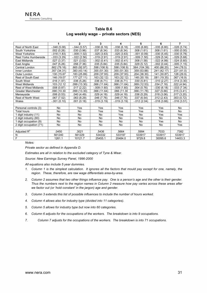
www.nera.com 31

Table B.6 Log weekly wage – private sectors (NES)

1 2 3 4 5 6 7 Rest of North East -.048 (5.08) -.044 (5.57) -.038 (6.16) -.038 (6.16) -.035 (6.80) -.035 (6.80) -.028 (5.74) South Yorkshire .002 (0.26) .030 (3.96) .037 (6.34) .033 (6.34) .008 (1.61) .008 (1.61) -.000 (0.00) West Yorkshire -.018 (1.83) -.009 (1.02) -.025 (3.63) -.025 (3.63) -.001 (0.09) -.030 (5.45) -.030 (5.78) Rest Yorks Humberside -.033 (3.29) -.022 (2.56) -.019 (2.91) -.019 (2.91) -.009 (1.50) -.029 (5.34) -.029 (5.68) East Midlands .027 (3.37) .021 (3.02) -.002 (0.41) -.002 (0.41) .008 (1.58) -.022 (4.99) -.024 (5.60) East Anglia .047 (5.26) .056 (7.36) .035 (5.84) .035 (5.84) .029 (5.12) -.002 (0.44) -.005 (1.15) Central London .662 (79.16) .665 (92.97) .598 (106.9) .598 (106.9) .564 (104.39) .400 (86.20) .344 (78.5) Inner London .357 (34.31) .383 (43.14) .355 (51.30) .355 (51.30) .359 (53.88) .241 (42.17) .221 (41.0) Outer London .130 (15.67 .183 (25.89) .209 (37.93) .209 (37.93) .204 (38.30) .141 (30.87) .128 (29.9) Rest of South East .146 (19.07 .177 (27.11) .163 (32.12) .163 (32.12) .148 (30.19) .081 (19.35) .067 (16.9) South West .016 (1.97) .036 (5.26) .036 (6.71) .036 (6.71) .030 (5.81) -.010 (2.27) -.014 (3.30) West Midlands .103 (12.12 .099 (13.30) .066 (11.64) .066 (11.64) .069 (12.53) .034 (7.16) .022 (4.94) Rest of West Midlands .008 (0.87) .017 (2.22) -.009 (1.60) -.009 (1.60) .004 (0.76) -.030 (6.18) -.033 (7.34) Greater Manchester .090 (10.30 .099 (13.30) .066 (11.64) .066 (11.30 .066 (11.78) .027 (5.66) .015 (3.41) Merseyside .006 (0.53) .040 (4.49) .029 (4.18) .029 (4.18) .036 (5.29) .018 (3.06) .017 (3.20) Rest of North West .067 (7.52) .063 (8.29) .046 (7.76) .046 (7.76) .037 (6.54) .012 (2.43) .003 (0.72) Wales -.001 (0.10) .001 (0.18) -.019 (3.19) -.019 (3.19) -.012 (2.04) -.018 (3.66) -.016 (3.51) Personal controls (3) No Yes Yes Yes Yes Yes No Total hours No No Yes Yes Yes Yes No 1 digit industry (11) No No No Yes No Yes Yes 2 digit industry (60) No No No No Yes No No 1 digit occupation (9) No No No No No Yes No 2 digit occupation (71) No No No No No No Yes Adjusted R2 .0450 .3021 .5436 .5664 .5994 .7033 .7382 N 561240 561229 534332 533197 533917 533917 533917 F 1261.1 10121.7 25455.1 20484.0 9729.8 30095.6 14453.3

Notes: Private sector as defined in Appendix D.


Source: New Earnings Survey Panel, 1996-2000

All equations also include 5 year dummies. 1. Column 1 is the simplest calculation. It ignores all the factors that mould pay except for one, namely, the



3. Column 3 extends this list of possible influences to include the number of hours worked.

4. Column 4 allows also for industry type (divided into 11 categories).

5. Column 5 allows for industry type but now into 60 categories.



www.nera.com 32

Table B.7 Public & private sectors (NES) – fixed effect estimation

1 2 3 4 5 6 Rest of North East -.026 (2.77) -.025 (2.66) -.021 (2.22) -.030 (3.49) -.030 (3.49) -.026 (3.07) South Yorkshire -.019 (1.81) -.016 (1.53) -.012 (1.20) -.020 (2.13) -.020 (2.13) -.015 (1.62) West Yorkshire -.043 (3.51) -.043 (3.48) -.039 (3.18) -.044 (3.90) -.044 (3.90) -.040 (3.63) Rest Yorks & Humberside -.031 (2.80) -.031 (2.85) -.030 (2.75) -.028 (2.75) -.028 (2.75) -.027 (2.72) East Midlands -.017 (1.69) -.016 (1.66) -.014 (1.45) -.015 (1.74) -.015 (1.74) -.013 (1.52) East Anglia -.003 (0.30) -.005 (0.43) -.001 (0.09) -.006 (0.59) -.006 (0.59) -.004 (0.36) Central London .180 (18.24) .178 (18.02) .172 (17.62) .159 (17.69) .159 (17.69) .152 (17.09) Inner London .133 (12.43) .134 (12.47) .128 (12.11) .119 (12.25) .119 (12.25) .115 (11.94) Outer London .055 (5.72) .058 (6.01) .060 (6.31) .057 (6.42) .057 (6.42) .060 (6.90) Rest of South East .032 (3.45) .033 (3.54) .034 (3.63) .031 (3.67) .031 (3.67) .032 (3.81) South West .002 (0.18) .000 (0.05) .001 (014) -.004 (0.43) -.004 (0.48) -.003 (0.38) West Midlands .033 (3.23) .033 (3.19) .036 (3.49) .036 (3.80) .036 (3.80) .037 (4.00) Rest of West Midlands -.005 (0.47) -.004 (0.39) .000 (0.14) .005 (0.53) .005 (0.53) .009 (0.98) Greater Manchester .018 (1.75) .018 (1.71) .020 (1.97) .018 (1.88) .018 (1.88) .019 (2.06) Merseyside -.004 (0.29) -.001 (0.10) -.000 (0.00) -.001 (0.09) -.001 (0.09) .002 (0.14) Rest of North West -.000 (0.03) -.001 (0.05) .004 (0.41) .006 (0.59) .006 (0.59) .009 (1.00) Wales -.008 (0.71) -.012 (1.03) -.007 (0.61) -.004 (0.35) -.004 (0.35) -.002 (0.21) 1 digit industry (9) No Yes No No Yes Yes 1 digit ocupation (8) No No Yes No No Yes Weekly wage Yes Yes Yes No No No Hourly wage No No No Yes Yes Yes Overall R2 .4347 .4487 .5788 .0253 .0500 .3134 N 646202 646202 646202 648596 646178 646178 F 12941.4 9285.9 7822.4 3037.1 2221.8 2038.1 # people fixed effects 212918 212660 212660 212904 212646 212646 Notes: This table looks at so-called fixed effects estimation, which means studying only those people who move region.



All equations also include 5 year dummies. 1. Column 1 gives raw wage differentials using weekly wages.

2. Column 2 augments that by adjusting for industry classification of workers, using a 9-industry breakdown.

3. Column 3 switches to an adjustment instead of workers’ occupation, using an 8-occupation breakdown.

4. Column 4 gives raw wage differentials using hourly wages.


6. Column 6 switches to an adjustment instead of workers’ occupation, using an 8-occupation breakdown as well as the 9-industry breakdown.

www.nera.com 33

Table B.8 Private sectors (NES) – fixed effect estimation

1 2 3 4 5 6* Rest of North East -.020 (1.84) -.019 (1.81) -.015 (1.39) -.025 (2.26) -.016 (1.64) -.025 (2.53) South Yorkshire -.014 (1.26) -.013 (1.16) -.012 (1.09) -.009 (0.78) -.007 (0.64) -.011 (1.04) West Yorkshire -.037 (2.77) -.038 (2.86) -.033 (2.48) -.041 (2.96) -.032 (2.64) -.041 (3.24) Rest Yorks & Humberside -.022 (1.88) -.023 (1.93) -.021 (1.78) -.015 (1.20) -.017 (1.56) -.014 (1.19) East Midlands -.014 (1.26) -.014 (1.29) -.013 (1.18) -.012 (1.08) -.006 (0.58) -.012 (1.15) East Anglia .001 (0.11) -.001 (0.09) .004 (0.33) .003 (0.25) .007 (0.61) -.001 (0.11) Central London .172 (15.74) .170 (15.54) .165 (15.23) .171 (15.29) .151 (15.21) .152 (14.68) Inner London .127 (10.64) .127 (10.67) .121 (10.29) .122 (10.02) .119 (11.01) .114 (10.14) Outer London .046 (4.27) .048 (4.45) .048 (4.57) .047 (4.28) .058 (5.97) .049 (4.90) Rest of South East .031 (2.96) .031 (2.95) .031 (2.99) .030 (2.82) .036 (3.82) .029 (2.92) South West .007 (0.66) .006 (0.51) .008 (0.76) .003 (0.24) .008 (0.74) -.002 (0.19) West Midlands .030 (2.68) .029 (2.59) .033 (2.91) .033 (2.85) .041 (3.99) .035 (3.25) Rest of West Midlands -.001 (0.09) -.001 (0.10) .003 (0.24) -.003 (0.24) .019 (1.79) .011 (1.00) Greater Manchester .018 (1.53) .017 (1.50) .021 (1.86) .019 (1.65) .024 (2.33) .019 (1.78) Merseyside .000 (0.01) .002 (0.17) -.000 (0.00) .000 (0.03) .011 (0.88) .002 (0.18) Rest of North West .008 (0.65) .007 (0.59) .012 (1.01) .006 (0.50) .019 (1.82) .011 (0.96) Wales -.008 (0.61) -.011 (0.87) -.002 (0.18) -.008 (0.58) .004 (0.32) -.002 (0.14) 1 digit industry (9) No Yes Yes Yes Yes Yes 1 digit ocupation (8) No No Yes Yes Yes Yes Weekly wage Yes Yes Yes No No No Hourly wage No No No Yes Yes Yes Overall R2 .4493 .4701 .5841 .5731 .3135 .3049 N 534342 533207 534342 490599 533190 490589 F 9923.1 7161.4 7778.9 5318.4 1676.6 1520.3 # people fixed effects 183193 183017 183193 173523 183007 173520 Notes:



Private sector in columns 4 & 6 as defined by IER at Warwick.

All equations also include 5 year dummies. 1. Column 1 gives raw wage differentials using weekly wages.


3. Column 3 switches to an adjustment instead of workers’ occupation, using an 8-occupation breakdown as well as the 9-industry breakdown.

4. Column 4 re-does that for hourly pay using a particular IER definition of the private sector.

5. Column 5 provides an alternative, using a different definition of private sector.

6. Column 6 re-does Column 4 using a particular IER definition of the private sector.

www.nera.com 34

Table B.9 Log weekly wage – private & public sector by occupation (LFS)

Managers & professionals

Technical non-manuals

Manual employees

Rest of North East -.060 (3.36) -.006 (0.45) -.016 (1.46) South Yorkshire -.054 (2.79) -.012 (0.82) -.025 (2.07) West Yorkshire .014 (0.82) .060 (4.71) .017 (1.56) Rest Yorks & Humberside -.074 (4.05) -.026 (1.79) -.019 (1.72) East Midlands -.025 (1.57) .021 (1.77) .002 (0.20) East Anglia -.004 (0.22) .031 (2.41) .015 (1.45) Central London .362 (22.78) .481 (38.35) .332 (23.70) Inner London .208 (12.37) .343 (25.28) .215 (17.10) Outer London .135 (8.57) .227 (18.55) .180 (17.04) Rest of South East .071 (4.84) .123 (11.15) .074 (8.04) South West -.038 (2.45) .026 (2.23) -.001 (0.07) West Midlands .007 (0.41) .050 (3.98) .037 (3.55) Rest of West Midlands -.037 (2.21) -.015 (1.19) -.014 (1.36) Greater Manchester -.011 (0.67) .045 (3.53) .025 (2.30) Merseyside -.017 (0.89) .044 (2.95) -.033 (2.55) Rest of North West -.052 (3.12) .010 (0.79) -.004 (0.41) Wales -.058 (3.47) -.010 (0.75) -.015 (1.51) Managers/professionals Yes No No Non-manuals - technical No Yes No Manual workers No No Yes Adjusted R2 .4463 .6297 .7340 N 66909 71252 124552 F 586.0 1469.7 2995.4 Notes:


Source: Labour Force Surveys, 1996-2001. All equations also include 5 year dummies. Controls are as in column 5 of Table B.1. Here the focus is on different segments of the working population. The following influences on pay have been factored out: age, gender, race, country of origin, hours of work, and length of job tenure.

www.nera.com 35

Table B.10 Log weekly wage – public & private sectors (LFS), 1993-5

1 2 3 4 5 6 Rest of North East -.040 (1.16) -.034 (1.20) -.028 (1.05) -.027 (1.03) -.017 (0.90) -.012 (0.64) South Yorkshire -.016 (0.44) -.014 (0.45) -.014 (0.48) -.014 (0.49) -.003 (0.17) .001 (0.09) West Yorkshire .051 (1.53) .067 (2.38) .057 (2.17) .056 (2.16) .032 (1.69) .031 (1.67) Rest Yorks & Humberside -.074 (2.08) -.062 (2.06) -.045 (1.60) -.044 (1.58) -.013 (0.65) -.014 (0.72) East Midlands -.018 (0.60) .009 (0.35) .015 (0.63) .015 (0.65) .007 (0.42) .009 (0.58) East Anglia .010 (0.32) .016 (0.57) .022 (0.84) .022 (0.84) .020 (1.10) .020 (1.08) Central London .764 (22.26) .702 (24.20) .575 (21.15) .574 (21.12) .436 (22.25) .427 (22.03) Inner London .468 (13.27) .472 (15.76) .370 (13.21) .370 (13.21) .321 (15.98) .323 (16.25) Outer London .282 (8.86) .295 (11.01) .249 (9.96) .249 (9.96) .221 (12.34) .216 (12.19) Rest of South East .108 (3.78) .128 (5.35) .096 (4.29) .096 (4.29) .099 (6.19) .099 (6.18) South West .001 (0.05) .016 (0.63) -.002 (0.09) -.001 (0.07) .009 (0.58) .008 (0.46) West Midlands .084 (2.61) .076 (22.80) .080 (3.16) .081 (3.18) .041 (2.24) .041 (2.27) Rest of West Midlands -.069 (2.09) -.044 (1.60) -.034 (1.34) -.034 (1.34) -.010 (0.59) -.010 (0.53) Greater Manchester .113 (3.42) .103 (3.75) .078 (3.05) .080 (3.10) .050 (2.72) .046 (2.53) Merseyside .068 (1.71) .078 (2.34) .067 (2.18) .068 (2.20) .046 (2.08) .043 (1.93) Rest of North West .014 (0.42) .036 (1.32) .023 (0.92) .023 (0.92) .015 (0.81) .014 (0.74) Wales -.025 (0.77) -.018 (0.67) -.024 (0.94) -.024 (0.9 -.020 (1.13) -.019 (1.02) Personal controls (3) No Yes Yes Yes Yes Yes Ethnic controls (8) No No Yes Yes Yes Yes Qualifications (31) No No No Yes Yes Yes Work controls (2) No No No No Yes Yes 1 digit industry (11) No No No No Yes No 2 digit industry (60) No No No No No Yes Adjusted R2 .0383 .3189 .4082 .4086 .6954 .7031 N 45873 45862 45850 45850 45749 45749 F 97.21 632.6 503.0 495.9 1296.2 1234.8 Notes:


This re-does Table B.1 for an earlier and shorter time period.

Source: Labour Force Surveys, 1993-1995, Q1 & Q3.

All equations also include two-year dummies.

1. Column 1 is the simplest calculation. It ignores all the factors that mould pay except for one, namely, the region. These, therefore, are raw wage differentials area-by-area.


3. Column 3 extends this list of possible influences to include ethnic background. It factors out from the wage equation a set of eight measures for a person’s race.

4. Column 4 allows for a long set of 31 different levels of qualification, as well as all the earlier factors. This is a particularly important step in providing a correct comparison of people between one region and another.


6. Column 6 adjusts for the number of hours the employee spends working, and the length of the person’s job tenure in the workplace. It also allows for which industry the person is employed within (grouping the country into approximately sixty different industries).

www.nera.com 36

Table B.11a Estimated area effects (%) for weekly wages using Labour Force Surveys


Public & private sectors (n=262,713) 55.0 33.5 21.3 10.0 Public sector (n=71, 221) 31.3 27.6 18.3 4.2 Private sector (n=190,917) 65.5 37.8 23.5 13.2 Private sector (n=190,917) 53.9 (merged) 23.6 13.2 Private sector (n=190,917) 38.6 (merged) 13.1 Private sector 1996-1998 (n=96,898) 64.0 35.3 23.2 12.0 Private sector 1999-2001 (n=94,019) 67.1 40.2 23.9 14.5 Males (n=129,288) 52.8 29.7 22.0 13.2 Females (n=133,425) 55.5 36.4 22.1 8.9 Degree or equivalent (n=42,404) 44.3 25.9 15.4 5.7 Higher education (n=26,216) 51.0 29.8 14.5 7.6 GCE A level or equivalent (n=58,564) 61.5 43.4 25.7 13.2 GCSE grade A-C or equivalent (n=64,141) 62.4 35.6 22.2 9.6 Other qualification (n=37,723) 64.8 36.3 25.0 12.1 No qualification (n=32,171) 53.0 28.1 24.2 11.6 Age<30 (n=67,075) 51.3 31.8 21.3 12.5 Age >=30 (n=195,638) 56.0 33.3 21.6 9.5 Manuals (n=98,780) 35.3 23.6 17.4 5.9 Non-manuals (n=162,731) 56.7 35.4 21.9 11.4 Notes: controls as in column 6 of Table B. 1 Sub-samples estimated using public and private sector data

Table B.11b Estimated area effects (%) for weekly wages using New Earnings Surveys


Public & private sectors (n=646,192) 38.1 24.1 14.2 6.3 Public sector (n=112,995) 23.0 20.1 15.7 2.2 Private sector (n=533,917) 41.1 24.7 13.7 6.9 Private sector 1996-1998 (n=317,353) 42.8 26.6 14.7 7.0 Private sector 1999-2000 (n=215,844) 38.5 21.8 12.3 6.7 Public & private excluding City of London (n=636,797)

34.0 24.2 14.3 6.4

Public & private including City of London (n=646,192)

34.0 (merged) 14.0 6.0

Public & private excluding City of London (n=636,797)

31.0 (merged) 14.0 6.0

Males (n=343,152) 43.3 23.0 14.3 9.5 Females (n=303,040) 43.5 28.3 18.0 7.0 Age<30 (n=163,182) 38.8 24.0 15.5 8.6 Age >=30 (n=483,010) 46.4 26.4 16.3 7.5 Manuals (n=234,293) 24.6 19.7 12.7 5.1 Non-manuals (n=411,819) 61.6 36.3 19.7 12.7 Notes: controls as in column 7 of Table B.5 Sub-samples estimated using public and private sector data

www.nera.com 37

APPENDIX C. AREA CODES

LAD County County # (Cwk) LADWK Region Tyne & Wear Gateshead Cleveland 5 362 NOTW Newcastle upon Tyne Cleveland 5 363 NOTW North Tyneside Cleveland 5 364 NOTW South Tyneside Cleveland 5 365 NOTW Sunderland Cleveland 5 366 NOTW Rest of the North Hartlepool Cleveland 1 344 NORO Lanagbaurgh on Tees Cleveland 1 345 NORO Middlesborough Cleveland 1 346 NORO Stockton on Tees Cleveland 1 347 NORO Allerdale Cumbria 2 338 NORO Barrow in Furness Cumbria 2 339 NORO Carlisle Cumbria 2 340 NORO Copeland Cumbria 2 341 NORO Eden Cumbria 2 342 NORO South Lakeland Cumbria 2 343 NORO Chester le Street Durham 3 348 NORO Darlington Durham 3 349 NORO Derwentside Durham 3 350 NORO Durham Durham 3 351 NORO Easington Durham 3 352 NORO Sedgefield Durham 3 353 NORO Teesdale Durham 3 354 NORO Wear Valley Durham 3 355 NORO Alnwick Northumberland 4 356 NORO Berwick upon Tweed Northumberland 4 357 NORO Blyth Valley Northumberland 4 358 NORO Castle Morpeth Northumberland 4 359 NORO Tynedale Northumberland 4 360 NORO Wansbeck Northumberland 4 361 NORO West Yorkshire Bradford West Yorkshire 8 296 YHMC Calderdale West Yorkshire 8 297 YHMC Kirklees West Yorkshire 8 298 YHMC Leeds West Yorkshire 8 299 YHMC Wakefield West Yorkshire 8 300 YHMC South Yorkshire Barnsley South Yorkshire 9 292 YHMC Doncaster South Yorkshire 9 293 YHMC Rotheram South Yorkshire 9 294 YHMC Sheffield South Yorkshire 9 295 YHMC Rest of Yorks Beverley Humberside 6 275 YHRO Boothferry Humberside 6 276 YHRO Cleethorpes Humberside 6 277 YHRO Glanford Humberside 6 279 YHRO Great Grimsby Humberside 6 280 YHRO Holderness Humberside 6 281 YHRO Kingston upon Hull Humberside 6 282 YHRO East Yorkshire Humberside 6 278 YHRO Scunthorpe Humberside 6 283 YHRO Craven North Yorkshire 7 284 YHRO Hambleton North Yorkshire 7 285 YHRO Harrogate North Yorkshire 7 286 YHRO Richmondshire North Yorkshire 7 287 YHRO Ryedale North Yorkshire 7 288 YHRO Scarborough North Yorkshire 7 289 YHRO Selby North Yorkshire 7 290 YHRO York North Yorkshire 7 291 YHRO

www.nera.com 38

LAD County County # (Cwk) LADWK Region East Midlands Amber Valley Derbyshire 10 235 EM Bolsover Derbyshire 10 236 EM Chesterfield Derbyshire 10 237 EM Derby Derbyshire 10 238 EM Erewash Derbyshire 10 239 EM High Peak Derbyshire 10 240 EM North East Derbyshire Derbyshire 10 241 EM South Derbyshire Derbyshire 10 242 EM Derbyshire Dales Derbyshire 10 243 EM Blaby Leicestershire 11 244 EM Hinckley & Bosworth Leicestershire 11 247 EM Charnwood Leicestershire 11 245 EM Harborough Leicestershire 11 246 EM Leicester Leicestershire 11 248 EM Melton Leicestershire 11 249 EM North West Leicestershire Leicestershire 11 250 EM Oadby & Wigston Leicestershire 11 251 EM Rutland Leicestershire 11 252 EM Boston Lincolnshire 13 253 EM East Lindsey Lincolnshire 13 254 EM Lincoln Lincolnshire 13 255 EM North Kesteven Lincolnshire 13 256 EM South Holland Lincolnshire 13 257 EM South Kesteven Lincolnshire 13 258 EM West Lindsey Lincolnshire 13 259 EM Ashfield Nottinghamshire 12 267 EM Bassetlaw Nottinghamshire 12 268 EM Broxtowe Nottinghamshire 12 269 EM Gedling Nottinghamshire 12 270 EM Mansfield Nottinghamshire 12 271 EM Newark & Sherwood Nottinghamshire 12 272 EM Nottingham Nottinghamshire 12 273 EM Rushcliffe Nottinghamshire 12 274 EM Corby Northamptonshire 12 260 EM Daventry Northamptonshire 14 261 EM East Norhamptonshire Northamptonshire 14 262 EM Kettering Northamptonshire 14 263 EM Northampton Northamptonshire 14 264 EM South Northamptonshire Northamptonshire 14 265 EM Wellingborough Northamptonshire 14 266 EM East Anglia Cambridge Cambridgeshire 15 99 EA East Cambridgeshire Cambridgeshire 15 100 EA Fenland Cambridgeshire 15 101 EA Huntingdonshire Cambridgeshire 15 102 EA Peterborough Cambridgeshire 15 103 EA South Cambridgeshire Cambridgeshire 15 104 EA Breckland Norfolk 16 105 EA Broadland Norfolk 16 106 EA Great Yarmouth Norfolk 16 107 EA Norwich Norfolk 16 108 EA North Norfolk Norfolk 16 109 EA South Norfolk Norfolk 16 110 EA Kings Lynn & West Norfolk Norfolk 16 111 EA Babergh Suffolk 17 112 EA Forrest Heath Suffolk 17 113 EA Ipswich Suffolk 17 114 EA Mid Suffolk Suffolk 17 115 EA St Edmundsbury Suffolk 17 116 EA Suffolk Coastal Suffolk 17 117 EA Waveney Suffolk 17 118 EA Central London Camden Central London 21 120 SEIL City of London Central London 21 119 SEIL Islington Central London 21 124 SEIL Lambeth Central London 21 126 SEIL Southwark Central London 21 129 SEIL Tower Hamlets Central London 21 130 SEIL City of Westminster Central London 21 132 SEIL Inner London Kensington & Chelsea Inner London 21 125 SEIL Lewisham Inner London 21 127 SEIL Newham Inner London 21 128 SEIL

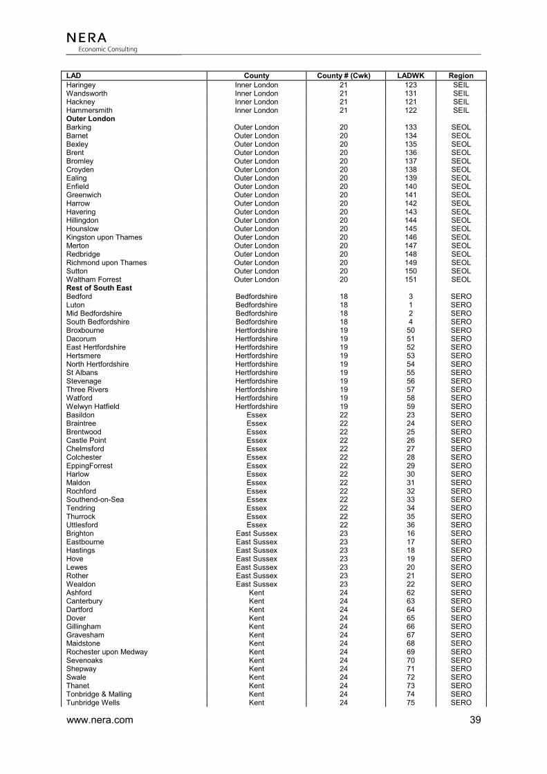
www.nera.com 39

LAD County County # (Cwk) LADWK Region Haringey Inner London 21 123 SEIL Wandsworth Inner London 21 131 SEIL Hackney Inner London 21 121 SEIL Hammersmith Inner London 21 122 SEIL Outer London Barking Outer London 20 133 SEOL Barnet Outer London 20 134 SEOL Bexley Outer London 20 135 SEOL Brent Outer London 20 136 SEOL Bromley Outer London 20 137 SEOL Croyden Outer London 20 138 SEOL Ealing Outer London 20 139 SEOL Enfield Outer London 20 140 SEOL Greenwich Outer London 20 141 SEOL Harrow Outer London 20 142 SEOL Havering Outer London 20 143 SEOL Hillingdon Outer London 20 144 SEOL Hounslow Outer London 20 145 SEOL Kingston upon Thames Outer London 20 146 SEOL Merton Outer London 20 147 SEOL Redbridge Outer London 20 148 SEOL Richmond upon Thames Outer London 20 149 SEOL Sutton Outer London 20 150 SEOL Waltham Forrest Outer London 20 151 SEOL Rest of South East Bedford Bedfordshire 18 3 SERO Luton Bedfordshire 18 1 SERO Mid Bedfordshire Bedfordshire 18 2 SERO South Bedfordshire Bedfordshire 18 4 SERO Broxbourne Hertfordshire 19 50 SERO Dacorum Hertfordshire 19 51 SERO East Hertfordshire Hertfordshire 19 52 SERO Hertsmere Hertfordshire 19 53 SERO North Hertfordshire Hertfordshire 19 54 SERO St Albans Hertfordshire 19 55 SERO Stevenage Hertfordshire 19 56 SERO Three Rivers Hertfordshire 19 57 SERO Watford Hertfordshire 19 58 SERO Welwyn Hatfield Hertfordshire 19 59 SERO Basildon Essex 22 23 SERO Braintree Essex 22 24 SERO Brentwood Essex 22 25 SERO Castle Point Essex 22 26 SERO Chelmsford Essex 22 27 SERO Colchester Essex 22 28 SERO EppingForrest Essex 22 29 SERO Harlow Essex 22 30 SERO Maldon Essex 22 31 SERO Rochford Essex 22 32 SERO Southend-on-Sea Essex 22 33 SERO Tendring Essex 22 34 SERO Thurrock Essex 22 35 SERO Uttlesford Essex 22 36 SERO Brighton East Sussex 23 16 SERO Eastbourne East Sussex 23 17 SERO Hastings East Sussex 23 18 SERO Hove East Sussex 23 19 SERO Lewes East Sussex 23 20 SERO Rother East Sussex 23 21 SERO Wealdon East Sussex 23 22 SERO Ashford Kent 24 62 SERO Canterbury Kent 24 63 SERO Dartford Kent 24 64 SERO Dover Kent 24 65 SERO Gillingham Kent 24 66 SERO Gravesham Kent 24 67 SERO Maidstone Kent 24 68 SERO Rochester upon Medway Kent 24 69 SERO Sevenoaks Kent 24 70 SERO Shepway Kent 24 71 SERO Swale Kent 24 72 SERO Thanet Kent 24 73 SERO Tonbridge & Malling Kent 24 74 SERO Tunbridge Wells Kent 24 75 SERO

www.nera.com 40

LAD County County # (Cwk) LADWK Region Elmbridge Surrey 25 81 SERO Epsom & Ewell Surrey 25 82 SERO Guildford Surrey 25 83 SERO Mole Valley Surrey 25 84 SERO Reigate & Barnstead Surrey 25 85 SERO Runnymede Surrey 25 86 SERO Spelthorne Surrey 25 87 SERO Surrey Heath Surrey 25 88 SERO Tandridge Surrey 25 89 SERO Waverley Surrey 25 90 SERO Woking Surrey 25 91 SERO Adur West Sussex 26 92 SERO Arun West Sussex 26 93 SERO Chichester West Sussex 26 94 SERO Crawley West Sussex 26 95 SERO Horsham West Sussex 26 96 SERO Mid Sussex West Sussex 26 97 SERO Worthing West Sussex 26 98 SERO Basingstoke & Deane Hampshire 27 37 SERO Eastleigh Hampshire 27 38 SERO Fareham Hampshire 27 39 SERO Gosport Hampshire 27 40 SERO Hart Hampshire 27 41 SERO Havant Hampshire 27 42 SERO New Forest Hampshire 27 43 SERO East Hampshire Hampshire 27 44 SERO Portsmouth Hampshire 27 45 SERO Rushmoor Hampshire 27 46 SERO Southampton Hampshire 27 47 SERO Test Valley Hampshire 27 48 SERO Winchester Hampshire 27 49 SERO Medina Isle of Wight 28 60 SERO South Wight Isle of Wight 28 61 SERO Bracknell Forrest Berkshire 31 5 SERO Newbury Berkshire 31 6 SERO Reading Berkshire 31 7 SERO Slough Berkshire 31 8 SERO Windsor & Maidenhead Berkshire 31 9 SERO Wokingham Berkshire 31 10 SERO Ayelsbury Vale Buckinghamshire 32 11 SERO South Buckinghamshire Buckinghamshire 32 12 SERO Chiltern Buckinghamshire 32 13 SERO Milton Keynes Buckinghamshire 32 14 SERO Wycombe Buckinghamshire 32 15 SERO Cherwell Oxfordshire 33 76 SERO Oxford Oxfordshire 33 77 SERO Vale of White Horse Oxfordshire 33 78 SERO South Oxfordshire Oxfordshire 33 79 SERO West Oxfordshire Oxfordshire 33 80 SERO South West Bournemouth Dorset 29 175 SW Christchurch Dorset 29 176 SW North Dorset Dorset 29 177 SW Poole Dorset 29 178 SW Purbeck Dorset 29 179 SW West Dorset Dorset 29 180 SW Weymouth & Portland Dorset 29 181 SW East Dorset Dorset 29 182 SW Kennet Wiltshire 30 194 SW North Wiltshire Wiltshire 30 195 SW Salisbury Wiltshire 30 196 SW Thamesdown Wiltshire 30 197 SW West Wiltshire Wiltshire 30 198 SW Bath Avon 34 152 SW Bristol Avon 34 153 SW Kingswood Avon 34 154 SW Wansdyke Avon 34 156 SW Woodspring Avon 34 157 SW Caradon Cornwall 35 158 SW Carrick Cornwall 35 159 SW Kerrier Cornwall 35 160 SW North Cornwall Cornwall 35 161 SW Penwith Cornwall 35 162 SW Isle of Scilly Cornwall 35 164 SW

www.nera.com 41

LAD County County # (Cwk) LADWK Region Restormel Cornwall 35 163 SW East Devon Devon 36 165 SW Exeter Devon 36 166 SW North Devon Devon 36 168 SW Plymouth Devon 36 169 SW South Hams Devon 36 170 SW Teignbridge Devon 36 171 SW Mid Devon Devon 36 167 SW Torbay Devon 36 172 SW Torridge Devon 36 173 SW West Devon Devon 36 174 SW Cheltenham Gloucestershire 37 183 SW Cotswold Gloucestershire 37 184 SW Forrest of Dean Gloucestershire 37 185 SW Gloucester Gloucestershire 37 186 SW Stroud Gloucestershire 37 187 SW Tewkesbury Gloucestershire 37 188 SW Mendip Somerset 38 189 SW Sedgemoor Somerset 38 190 SW Taunton Deane Somerset 38 191 SW West Somerset Somerset 38 192 SW South Somerset Somerset 38 193 SW West Midlands Metropolitan Birmingham West Midlands 43 228 WMMC Coventry West Midlands 43 229 WMMC Dudley West Midlands 43 230 WMMC Sandwell West Midlands 43 231 WMMC Solihull West Midlands 43 232 WMMC Walsall West Midlands 43 233 WMMC Wolverhampton West Midlands 43 234 WMMC Rest of West Midlands Bromsgrove Hereford&Worcester 39 199 WMRO Hereford Hereford&Worcester 39 200 WMRO Leominster Hereford&Worcester 39 201 WMRO Malvern Hills Hereford&Worcester 39 202 WMRO Redditch Hereford&Worcester 39 203 WMRO South Herefordshire Hereford&Worcester 39 204 WMRO Worcester Hereford&Worcester 39 205 WMRO Wychavon Hereford&Worcester 39 206 WMRO Wyre Forrest Hereford&Worcester 39 207 WMRO Bridgnorth Shropshire 40 208 WMRO North Shropshire Shropshire 40 209 WMRO Oswestry Shropshire 40 210 WMRO Shrewsbury & Athcam Shropshire 40 211 WMRO South Shropshire Shropshire 40 212 WMRO The Wrekin Shropshire 40 213 WMRO Cannock Chase Staffordshire 41 214 WMRO East Staffordshire Staffordshire 41 215 WMRO Lichfield Staffordshire 41 216 WMRO Newcastle under Lyme Staffordshire 41 217 WMRO South Staffordshire Staffordshire 41 218 WMRO Stafford Staffordshire 41 219 WMRO Staffordshire Moorlands Staffordshire 41 220 WMRO Stoke-on-Trent Staffordshire 41 221 WMRO Tamworth Staffordshire 41 222 WMRO North Warwickshire Warwickshire 42 223 WMRO Nuneaton & Bedworth Warwickshire 42 224 WMRO Rugby Warwickshire 42 225 WMRO Stratford upon Avon Warwickshire 42 226 WMRO Warwick Warwickshire 42 227 WMRO Greater Manchester Bolton Greater Manchester 46 309 NWMC Bury Greater Manchester 46 310 NWMC Manchester Greater Manchester 46 311 NWMC Oldham Greater Manchester 46 312 NWMC Rochdale Greater Manchester 46 313 NWMC Salford Greater Manchester 46 314 NWMC Stockport Greater Manchester 46 315 NWMC Tameside Greater Manchester 46 316 NWMC Trafford Greater Manchester 46 317 NWMC Wigan Greater Manchester 46 318 NWMC Merseyside Knowsley Merseyside 47 319 NWMC Liverpool Merseyside 47 320 NWMC

www.nera.com 42

LAD County County # (Cwk) LADWK Region St Helens Merseyside 47 321 NWMC Sefton Merseyside 47 322 NWMC Wirral Merseyside 47 323 NWMC Rest of North West Chester Cheshire 44 301 NWRO Congleton Cheshire 44 302 NWRO Crewe & Nantwich Cheshire 44 303 NWRO Ellesmere Port & Neston Cheshire 44 304 NWRO Halton Cheshire 44 305 NWRO Macclesfield Cheshire 44 306 NWRO Vale Royal Cheshire 44 307 NWRO Warrington Cheshire 44 308 NWRO Blackburn Lancashire 45 309 NWRO Blackpool Lancashire 45 310 NWRO Bunley Lancashire 45 311 NWRO Chorley Lancashire 45 312 NWRO Fylde Lancashire 45 313 NWRO Hyndburn Lancashire 45 314 NWRO Lancaster Lancashire 45 315 NWRO Pendle Lancashire 45 316 NWRO Preston Lancashire 45 317 NWRO Ribble Valley Lancashire 45 318 NWRO Rossendale Lancashire 45 319 NWRO South Ribble Lancashire 45 320 NWRO West Lancashire Lancashire 45 321 NWRO Wyre Lancashire 45 322 NWRO Wales Alyn & Deeside Clwyd 48 367 WA Colwyn Clwyd 48 368 WA Delyn Clwyd 48 369 WA Glyndwr Clwyd 48 370 WA Rhuddlan Clwyd 48 371 WA Wrexham Maelor Clwyd 48 372 WA Carmathen Dyfed 49 373 WA Ceredigion Dyfed 49 374 WA Dinefwr Dyfed 49 375 WA Llanelli Dyfed 49 376 WA Preseli Pembrokeshire Dyfed 49 377 WA South Pembrokeshire Dyfed 49 378 WA Blaenau Gwent Gwent 50 379 WA Islwyn Gwent 50 380 WA Monmouth Gwent 50 381 WA Newport Gwent 50 382 WA Torfaen Gwent 50 383 WA Aberconwy Gwynedd 51 384 WA Arfon Gwynedd 51 385 WA Dwyfor Gwynedd 51 386 WA Meirionnydd Gwynedd 51 387 WA Ynys Mon-Isle of Anglesey Gwynedd 51 388 WA Cynon Valley Mid Glamorgan 52 389 WA Merthyr Tydfil Mid Glamorgan 52 390 WA Ogwr Mid Glamorgan 52 391 WA Rhondda Mid Glamorgan 52 392 WA Rhymney Valley Mid Glamorgan 52 393 WA Taff-Ely Mid Glamorgan 52 394 WA Brecknock Powys 53 395 WA Radnorshire Powys 53 396 WA Montgomeryshire Powys 53 397 WA Cardiff South Glamorgan 54 398 WA Vale of Glamorgan South Glamorgan 54 399 WA Port Talbot West Glamorgan 55 400 WA Lliw Valley West Glamorgan 55 401 WA Neath West Glamorgan 55 402 WA Swansea West Glamorgan 55 403 WA Strathclyde Argyll & Bute Strathclyde 63 404 SCSC Bearsden & Milngavie Strathclyde 63 405 SCSC Clydebank Strathclyde 63 406 SCSC Cumbernauld & Kilnsyth Strathclyde 63 407 SCSC Cumbernauld & Kilnsyth Strathclyde 63 408 SCSC Cunninghame Strathclyde 63 409 SCSC Dumbarton Strathclyde 63 410 SCSC East Kilbride Strathclyde 63 411 SCSC Eastwood Strathclyde 63 412 SCSC

www.nera.com 43

LAD County County # (Cwk) LADWK Region Glasgow City Strathclyde 63 413 SCSC Hamilton Strathclyde 63 414 SCSC Inverclyde Strathclyde 63 415 SCSC Kilmarnock & Loudon Strathclyde 63 416 SCSC Kyle & Carrick Strathclyde 63 417 SCSC Clydesdale (Lanark) Strathclyde 63 418 SCSC Monklands Strathclyde 63 419 SCSC Motherwell Strathclyde 63 420 SCSC Renfrew Strathclyde 63 421 SCSC Strathkelvin Strathclyde 63 422 SCSC Rest of Scotland Berwickshire Borders 56 423 SCRO Ettrick & Lauderdale Borders 56 424 SCRO Roxburgh Borders 56 425 SCRO Tweedale Borders 56 426 SCRO Clackmanion Central 57 427 SCRO Falkirk Central 57 428 SCRO Stirling Central 57 429 SCRO Annandale & Eskdale Dumfries & Galloway 58 430 SCRO Nithsdale Dumfries & Galloway 58 431 SCRO Stewartry Dumfries & Galloway 58 432 SCRO Wigtown Dumfries & Galloway 58 433 SCRO Dunfermline Fife 59 434 SCRO Kirkcaldy Fife 59 435 SCRO North East Fife Fife 59 436 SCRO Aberdeen City Grampian 60 437 SCRO Banff & Buchan Grampian 60 438 SCRO Gordon Grampian 60 439 SCRO Kincardine & Deeside Grampian 60 440 SCRO Moray Grampian 60 441 SCRO Badenoch & Strathspey Highland 61 442 SCRO Caithness Highland 61 443 SCRO Inverness Highland 61 444 SCRO Lochaber Highland 61 445 SCRO Nairn Highland 61 446 SCRO Ross & Cromarty Highland 61 447 SCRO Skye & Lochalsh Highland 61 448 SCRO Sutherland Highland 61 449 SCRO East Lothian Lothian 62 450 SCRO Edinburgh City Lothian 62 451 SCRO Midlothian Lothian 62 452 SCRO West Lothian Lothian 62 453 SCRO Angus Tayside 64 454 SCRO Dundee City Tayside 64 455 SCRO Perth & Kinloss Tayside 64 456 SCRO Orkney Islands Northern & Western 65 457 SCRO Shetland Islands Northern & Western 65 458 SCRO Western Isles Northern & Western 65 459 SCRO

www.nera.com 44

APPENDIX D. OCCUPATIONAL CODES

To do the statistical work described above, we have to have clear definitions of the taxonomic differences in the data between those who work in the public versus the private parts of the economy. Such a taxonomy is a compromise, because it is not possible with conventional data sources to be certain in every case whether, as just one example, a dental nurse is employed by a private dentist rather than a National Health Service dentist. The Appendix sets out the standard Occupation Codes (1992 definitions) that were used to define public sector workers compared to private sector workers. The codes run from #102 Local government officers through to #940 postal workers and mail sorters.

1992 Occupation codes used to define the public sector

102 Local government officers (administrative & executive functions) 103 General administrators; national government (HEO to Senior Principal/Grade 6) 132 Civil Service executive officers 152 Police officers (inspector & above) 153 Fire service officers (station officer & above) 154 Prison officers (principal officer & above) 155 Customs & excise, immigration service officers (customs: chief preventive officer & above; excise: surveyor & above 230 University & polytechnic teaching professionals 231 Higher & further education teaching professionals 232 Education officers, school inspectors 233 Secondary (& middle school deemed secondary) education teaching professionals 234 Primary (& middle school deemed primary) & nursery education teaching professionals 235 Special education teaching professionals 239 Other teaching professionals nes 240 Judges & officers of the court 293 Social workers, probation officers 340 Nurses 341 Midwives 342 Medical radiographers 343 Physiotherapists 344 Chiropodists 345 Dispensing opticians 346 Medical technicians, dental auxiliaries 347 Occupational & speech therapists, psychotherapists, therapists nes 348 Environmental health officers 349 Other health associate professionals nes 370 Matrons, house parents 371 Welfare, community & youth workers 400 Civil Service administrative officers & assistants 401 Local government clerical officers & assistants 451 Legal secretaries 610 Police officers (sergeant & below) 611 Fire service officers (leading fire officer & below) 612 Prison service officers (below principal officer) 613 Customs & excise officers, immigration officers (customs: below chief preventive officer; excise: below surveyor) 614 Traffic wardens 640 Assistant nurses, nursing auxiliaries 641 Hospital ward assistants 642 Ambulance staff 643 Dental nurses 644 Care assistants & attendants 652 Educational assistants 659 Other childcare & related occupations nes 940 Postal workers, mail sorters

www.nera.com 45

APPENDIX E. FIXED EFFECTS & EARLIER RELATED WORK

Fixed-effects techniques fall within a statistical family called panel estimators.13 As explained in NERA (1998), a fixed-effects regression equation can be thought of as follows:

Think about Ms Z’s pay. This is likely to depend on:

i. the education, age ,background, and so on, of Ms Z; and

ii. subtle personality characteristics of Ms Z, such as her determination and drive, which through the years tend to be fixed characteristics of Ms Z.

The first category causes no real problems for statisticians and economists. Factors like age and education can be measured. It is the second category (the level of, for example, drive) that leads to difficulties for normal statistical methods. Because such things are not measurable in a normal survey, an interviewer cannot record them in a questionnaire. Fixed-effect techniques were designed precisely to try to allow for subtle ‘fixed’ factors like (ii).

The idea of fixed-effects methods is to examine what happens to a person’s wage when he or she changes regions. By contrast, cross-section analysis calculates regional pay by taking averages (holding other factors constant, of course) of the wages earned by everyone living in each UK region. Both methods attempt to measure true wage differences from one area to another.

Earlier research papers on the Area Cost Adjustment were produced by Professor David Bell (for SIGOMA) and Drs Denny and Preston (for the Department of Environment, Transport and the Regions). These suggested that fixed-effects methods could be used by the DETR to calculate the Labour Cost Adjustment (LCA). David Bell’s paper did some exploratory calculations using the New Earnings Survey. He found that fixed-effects models gave lower – in some cases up to 30 percentage points lower - regional wage coefficients than found in cross-sections.

13 Some authors have argued that instead of a fixed effects estimator a random effects estimator should be used. David Bell has made two quite strong arguments against using a random effects model with the NESPD – bias and heteroscedasticity (Wilson et al, 2001 Annex C, page 103).

i) Bias. The random effects model is more efficient than fixed effects only if the unobserved individual effects are uncorrelated with the observed regressors. There is no a priori reason to believe that this is the case with the NESPD which has a very limited set of potential explanatory variables. If the correlation is in fact non-zero, then the fixed effects estimator is inefficient but consistent, whereas the random effects estimator is inconsistent.

ii) Heteroscedasticity. The NESPD is a highly unbalanced panel – the amount of observations on each individual is highly variable. This poses no particular problems for the fixed effects estimator, but in the random effects case means that the estimator of the regression variance is biased due to heteroscedasticity in the variance components. For this not to be a problem requires that the length of time an individual is present in the panel is randomly distributed (see H.J. Greene’s Econometric Analysis (2000), Prentice Hall, page 578) which is likely to be a strong assumption in the case of the NESPD.

www.nera.com 46

Professor Bell’s report is in the same theoretical spirit as the Elliott Review. It follows the avenue of research known as the general labour market (GLM) approach. However, Professor Elliott’s committee advised against using fixed effects panel methods for technical reasons.

A practical difficulty with fixed-effects techniques is that they have hardly ever been applied to study workers’ wages in the United Kingdom. One paper is by David Bell and coauthors, in 1998, in the Oxford Bulletin of Economics and Statistics. There is also some related research on company panels by, for example, Hildreth and Oswald (1997). But currently in the UK this particular research field is not very well developed.

Perhaps the simplest way to estimate a fixed-effects wage equation is to include in an otherwise standard regression a separate dummy variable for each person. If 5000 people are observed for each of five years, for example, a regression equation can be estimated on a sample of 25,000 observations. A cross-section analysis could in principle be done, but panel estimation takes a further step. Apart from normal independent variables - such as age, qualifications, region, etc - five thousand additional independent variables are included (one for each person). Such dummies are thought of as measuring “person-specific effects”. These encapsulate drive, punctuality, conscientiousness, and any other personality trait.

Crucially, however, this form of estimation has now allowed – because there is a dummy variable for each individual - for the unchanging characteristics of people. Factors that are innate are automatically held constant by the statistical technique. The fixed-effects estimator should therefore allow more reliable inferences than a cross-section analysis that leaves out the five thousand dummy variables.

A difficulty is that fixed-effects results are likely to produce regional differentials that are biased down. Such bias is to be expected for at least two reasons:

• some people will move region while keeping the same job, which, because we are measuring area as their home location, will wrongly make it appear that pay does not depend on geographical area; and

• there will be some errors in people’s recorded region (simple coding mistakes, and conceptual mistakes among those living close to boundaries).

A source of bias in the panel estimates produced by Bell arises because of ‘sample selection’. This is a way of saying that Professor Bell was studying a special – not wholly random - group of workers. Selection bias can exist for a number of reasons. It is likely to be of particular concern here - as the extent of the selection is likely to vary significantly by region.

1. The New Earnings Survey data files exclude individuals who earn less than the minimum earnings required to pay national insurance.

2. Individuals who work in new firms are likely to be excluded from the NES sample (but not the LFS sample) because of the difficulty involved in maintaining an up-to-date sampling frame. This is always a problem for statistical agencies: they struggle to

www.nera.com 47

make sample of firms representative. This is why the most believable estimates in labour market research are usually derived from samples of individuals rather than samples of firms or workplaces.

3. Individuals who join a firm during a particular year and are not present at the sampling data in the NES will be excluded. They will have a much lower probability of being excluded from the LFS because this survey is taken quarterly. This means that the NES sample in a particular year is likely to be unrepresentative of new entrants to the labour market as well as of individuals who have entered work from a spell of either unemployment or being out of the labour force.

4. Most importantly, if, as we have shown, movers are not a random draw from the wage distribution, this is likely to result in a selection bias. It appears that movers are more qualified and younger than stayers. Conceptually it is hard to think of a suitable way to control for this since the NES contains only a very few variables (none of which is a likely candidate as an instrument). Hence it is hard to see how this problem of endogeneity bias of who moves could ever be solved.

In addition, if there is any measurement error in the way regions are identified, this will further bias the panel results downward. Gregg Lewis, in his famous analysis of the effects of unions on relative wages, found that estimates derived from panel data were considerably lower than those arising from OLS estimates using cross-section data files (though he was not studying region dummy variables). He argued persuasively "misclassification of workers by union status may account for all of the average difference between panel and cross-section estimates" (1986, p.5).

It is unclear to what extent there is measurement error in the region identifiers from year to year in the NES sample. What if an individual worked for a firm in area A and was paid from a central pay office and then moved to Area B but was still classified as being paid from the same pay office; would that move be identified? To what extent are reported moves across regions correlated with actual moves? Inaccuracies in the status-change data are likely to lead to a downward bias in estimated region effects using panel data.

We conclude that the small regional pay relativities derived from fixed effects methods are likely to be biased downwards and are not a reliable guide to wage relativities. Fixed effects methods are not sufficiently developed and tested to be used in estimating the labour cost component of ACA.

www.nera.com 48

REFERENCES

Andrews, Martin, Bell, David, and Upward, Richard. February 1998. “Union Coverage Differentials. Some Estimates for Britain using the New Earnings Survey Panel Data-Set”. Oxford Bulletin of Economics and Statistics, 60.

Bell, David. July 1998. Further Research on the Area Cost Adjustment: A Report for SIGOMA.

Denny, Kevin, and Preston, Ian. June 1998. Report of Advisory Panel on the Use of Fixed Effects Methods in Area Cost Adjustment.

Peter Dolton and Wilbert van der Klaauw. March 1995. Leaving Teaching in the UK: A Duration Analysis. The Economic Journal, Volume 105, p431-444.

Elliott, R.F., McDonald, D., R. MacIver. July 1996. Review of the Area Cost Adjustment, Waverley Press, University of Aberdeen and the Department of Environment.

Freeman, Richard B. January 1984. “Longitudinal Analyses of the Effects of Trade Unions”. Journal of Labor Economics, Volume 2(1). p1-26.

Hamermesh, Daniel, 1998, ‘The Art of Labormetrics’, University of Texas working paper, in Handbook of Econometrics, Vol.5, North-Holland.

Hildreth, Andrew and Oswald, Andrew. October 1997. ‘Wages and Rent Sharing: Evidence from Company and Establishment Panels’, Journal of Labor Economics, Volume 15, p318-337.

Lewis, H.G. 1986. Union Relative Wage Effects - A Survey. University of Chicago Press.

London Economics, Research Project A: The Review of the Area Cost Adjustment, 1996, Supplementary Annex.

NERA. August 1998. Area Cost Adjustment: Specific Cost Approach.

Wilson, R., Davies, R., Green, A., Owen, D. and P. Elias. October 2001. “Spatial Variations in Labour Costs: 2001 Review of the Staff Market Forces factor”, mimeo, Institute for Employment Research, University of Warwick.

estimated regional wage relativities for england a …blnchflr/papers/4975.pdf · estimated...

Documents