establishment of steering circuits and evaluation of oil...
TRANSCRIPT

Establishment of steering circuits and evaluation of oil temperature Master’s Thesis in the Automotive Engineering Master’s program
BRUNO GOUNIN Department of Applied Mechanics Division of Vehicle Safety CHALMERS UNIVERSITY OF TECHNOLOGY Göteborg, Sweden 2009 Master’s Thesis 2009:44


MASTER’S THESIS 2009:44
Establishment of steering circuits and evaluation of oil temperature
Master’s Thesis in the Automotive Engineering Master’s program
BRUNO GOUNIN
Department of Applied Mechanics Division ofVehicle Safety
CHALMERS UNIVERSITY OF TECHNOLOGY
Göteborg, Sweden 2009
Establishment of a thermal model of directions circuits and evaluation of oil temperature Master’s Thesis in the Automotive Engineering Master’s program BRUNO GOUNIN
© BRUNO GOUNIN2009
Master’s Thesis 2009:44 ISSN 1652-8557 Department of Applied Mechanics Division of Vehicle Safety Chalmers University of Technology SE-412 96 Göteborg Sweden Telephone: + 46 (0)31-772 1000 Department of Applied Mechanics Göteborg, Sweden 2009


CHALMERS, Applied Mechanics, Master’s Thesis 2009:44
I
Establishment of a thermal model of directions circuits and evaluation of oil temperature Master’s Thesis in the Automotive Engineering Master’s program BRUNO GOUNIN Department of Applied Mechanics Division of Vehicle Safety Chalmers University of Technology
ABSTRACT
The master thesis has been performed for Volvo 3P on the site of Lyon in France, and in the premises of the design office front and rear axle installation of the product development department. This unit is in charge of the conception, the design and the production of the chassis and of the power steering system of all the trucks of the Volvo AB group.
The sizing of the circuits is currently grounded on the experience of the member of the design office. Each new steering circuit has to follow a serial of test in different condition of utilization in order to be validated by Volvo and its suppliers. To secure the design process, the introduction of a simulation method in the design process of steering circuits has been wished. The simulation tool is intended to need input data simple enough so that it can be used in the early development stage of a design process. It has been decided to simulate static tests, when the engine runs at constant speed without air circulation. The tool has to be able to predict the oil temperature with an error of 10%. To validate the tool, the results need to be correlated on different circuit architectures. Finally the tool needs to be confronted to reality by comparing the prediction with measurement lead on a prototype vehicle.
The software Amesim has been chosen to develop the simulation tool. In fact a pre study of the problem has shown that different scientific domains have to be taken in account to model the steering oil temperature evolution. In particular the heat transfers and the fluid mechanic have to be considered. Based on the bond graph theory, Amesim is a convenient software to model complex physical phenomena. To model correctly a steering circuit, the key components have to be identified and characterized in static functioning. The pump, the oil tank, the pipes and the steering gear are the principle components of interest. Their pressure losses and heat transfers have been thoroughly defined in static condition so as to obtain pertinent results.
The Simulations have been realized on two completely different steering circuits, and the results obtain are encouraging. Four test cases have been studied on a Premium Lancer LC 8x4 MD 11 with results differences inferior to 5% with tests. Two test cases have also been studied on a Premium 4x2 MD11 and have given results with errors inferior to 7% compared to reality. Nevertheless it has been impossible to confront the models with the reality due to delaying of testing because of the international financial crisis. Then the steering gear hydraulic path has been identified as an influencing parameter on the oil temperature and has been approximated. A close work with the suppliers must lead in the future to a better knowledge of that component. Finally the influence of the surrounding temperature has also been highlighted. The next step is to consider the fan strategy in the modelling of steering circuit so as to enhance the accuracy of the model. Finally it is necessary to confront the simulation to the reality in order to validate the modelling method.

CHALMERS, Applied Mechanics, Master’s Thesis 2009:44
II

CHALMERS, Applied Mechanics, Master’s Thesis 2009:44 III
Contents ABSTRACT I
CONTENTS III
PREFACE VI
NOTATIONS VII
1 INTRODUCTION 2
1.1 Background 2
1.2 Task description 2
1.3 Expected outcomes 2
2 THE VOLVO WAY 3
2.1 Organisation 3 2.1.1 The Volvo group 3 2.1.2 Volvo 3P 3 2.1.3 Front and rear axle installation 4
2.2 Global Development process 4
2.3 Projects development 5 2.3.1 The GDP cornerstones 5 2.3.2 The project management way 6 2.3.3 Secure the Power Steering Design 6
3 PRESENTATION OF THE SUBJECT 7
3.1 Scope 7
3.2 Validation by testing 8
3.3 Development of a simulation tool 9
4 HYDRAULIC STEERING CIRCUIT 10
4.1 Steering assistance system 10
4.2 Functioning 11
4.3 Thermal exchanges 12 4.3.1 Conduction 12 4.3.2 Convection 13
5 AMESIM PRESENTATION 15
5.1 Theory 15
5.2 Software environment 16
5.3 Presentation of the libraries 16 5.3.1 Thermal hydraulic library 17 5.3.2 Thermal library 19

CHALMERS, Applied Mechanics, Master’s Thesis 2009:44 IV
5.3.3 Thermal pneumatic library 20
6 DEVELOPMENT OF A MODEL 22
6.1 Modelling approach 22
6.2 Characterization of materials and fluids 22 6.2.1 Presentation 22 6.2.2 Choice of the submodels 25
6.3 The piping 29 6.3.1 Theory of thermal exchanges 29 6.3.2 Modelling with Amesim 31
6.4 The pump 35
6.5 The steering gear 37 6.4.1 Functioning 37 6.4.2 The steering gear modelling 37
7 PRESENTATION OF MODELS AND SIMULATIONS 41
7.1 Introduction 41
7.2 Complete model example 42
7.3 Simulations 44 7.3.1 Simulation settings 44 7.3.2 Data processing 44
7.4 Presentation of results 45 7.4.1 Premium Lancer LC 8x4 MD11 left hand drive 45 7.4.2 Premium 4x2 MD11 left hand drive 46
8 CONCLUSION AND RECOMMENDATIONS 47
8.1 Conclusion 47
8.2 Recommendations 47 8.2.1 Characterisation of the steering gear 47 8.2.2 Surrounding temperature control 47
9 REFERENCES 48
APPENDIX 1 CONDUCTION HEAT TRANSFER 49
APPENDIX 2 THE DIMENSIONLESS NUMBERS 50
APPENDIX 3 NUSSELT CORRELATIONS 51
APPENDIX 4 EXAMPLES OF CIRCUIT OVERVIEW 52
APPENDIX 5 SOLID THERMAL PROPERTIES 53

CHALMERS, Applied Mechanics, Master’s Thesis 2009:44 V
APPENDIX 6 LIQUID THERMAL PROPERTIES 54
APPENDIX 7 GAS THERMAL PROPERTIES 55
APPENDIX 8 DEFINITION OF THE STARMATIC 3 OIL 56
APPENDIX 9 FUNCTIONING OF THE CONTROL FLOW VALVE 57
APPENDIX 10 EXAMPLE OF STEERING OIL TEMPERATURE MEASUREMENT 58
CHALMERS, Applied Mechanics, Master’s Thesis 2009:44 VI
Preface The development work has been carried out within the design office “front and rear axle installation” facilities of Volvo 3P on the Lyon site from November 2008 to April 2009. The work is a foundation of a calculation tool dedicated to the development of power steering system as to improve the development process.
I have to thank especially Jean-Marc BLOND, responsible for the front axle installation, and Philippe BOITARD, responsible for the design office calculations, to have proposed me an exciting thesis subject. In fact the opportunity to work on the development of a calculation tool, taking place very soon in a project development process, has been very instructive for me in the understanding of the stakes of a design office in the automotive engineering field. Their supervising and their support in my day-to-day work have been a key to success in the realization of the project, and have allowed me to learn a lot. My thanks extends to all the design office members for their pleasant welcoming and availability which has enabled me to integrate quickly, and for having be able to give me some time to answer my questions. I would like to thank especially Olivier TEIL and Olivier VILLOT, responsible of the development of the power steering system components, for their support.
Lyon May 2009
Bruno Gounin

CHALMERS, Applied Mechanics, Master’s Thesis 2009:44 VII
Notations Roman upper case letters
A Variable notation for heat exchange area (m²) L Notation for length (m) T Variable notation for temperature (K) Nu Variable notation for Nusselt number Pr Variable notation for Prandlt number Re Variable notation for Reynolds number Gr Variable notation for Grashof number Cdim Notation for characteristic dimension of heat exchange (m) Cp Variable notation for thermal capacity (J/K/kg) V Variable notation for flow velocity (m/s) D Notation for hydraulic diameter (m) Q Variable notation for volumetric flow rate (m3/s)
Roman lower case letters
d Notation for distance (m) dext Notation for external diameter (m) dint Notation for internal diameter (m) h Variable notation for convective heat exchange coefficient (W/m²/K) dmh Variable notation for enthalpy flow rate (J/s) g Notation for the acceleration due to gravity (m.s-2) r Notation for the perfect gas constant (J/kg/K) p Variable notation for pressure (Pa)
Greek case letters
Φ Variable notation for heat flux (W) ΔT Variable notation for something (K) µ Variable notation for absolute viscosity (Pa.s) ν Variable notation for kinematic viscosity (m²/s) λ Variable notation for thermal conductivity (w/m/K) β Variable notation for bulk modulus (Pa)
α Variable notation for volumetric expansion coefficient (K-1) ζ Notation for friction factor ρ Variable notation for density (kg/m3) Δp Variable notation for pressure drop (Pa)
σ Notation for Stefan-Boltzmann constant

CHALMERS, Applied Mechanics, Master’s Thesis 2009:44
I

CHALMERS, Applied Mechanics, Master’s Thesis 2009:44
2
1 Introduction 1.1 Background In 2007, Raphael Scarfo, student in last year of the INSA Lyon (engineering school), has carried out a first study on the development of a simulation tool dedicated to the sizing of the steering gear circuit. At that time a major issue occurred in the validation process of a steering gear circuit, and an action plan has been set to prevent any similar mistake. The wish to introduce thermal and hydraulic calculations in the design of the function was born.
That first study allowed identifying the main parameters to take into account in the hydraulic and heat transfer domains to model a steering gear circuit. Then the definition of the simulation test to carry on that model has been defined in comparison with a common physical test carry on a vehicle prototype in order to readjust the model to the reality. At least a broad set of testing has been carried out on a vehicle equipped with pressure and thermal sensors.
1.2 Task description The task assigns for the master thesis is to develop a correlated simulation tool of steering oil temperature prediction on different steering circuit architecture. The simulation tool needs to have input data simple enough so that the engineers could use it in the early development stage of the steering function. The key points are to identify the most sensitive input data that are complex to handle without data acquisition and to model the physical phenomena influencing the temperature evolution of the steering oil flowing through the circuit in functioning.
1.3 Expected outcomes The simulation tool is intended to predict the oil temperature of a power steering circuit in development with an error of 10%. Tests realized on prototype vehicle are intended to be confronting with the prediction of the simulation tool. The major physical phenomena taking place around a circuit are intended to be identified, control and model. Finally a utilization notice is expected to be delivering to the design office “front and rear axle installation” so that the simulations and calculations could progressively integrate the design process of the steering function.

CHALMERS, Applied Mechanics, Master’s Thesis 2009:44
3
2 The Volvo way 2.1 Organisation
2.1.1 The Volvo group
The Volvo group is offering a range of transport solutions to its customers around the world. A broad range of trucks, buses and construction equipments is proposed. This world-class group is organized in product-related business areas and supporting business units. This organization permits companies to work closely with their customers and efficiently utilize Group-wide resources. The Figure 1 illustrates that organization.
Figure 1 Volvo group organization
The business units are organized globally and combine expertise in key areas. They have the overall responsibility for product planning and purchasing, and for developing and delivering components, subsystems, services and support to the group’s business areas.
2.1.2 Volvo 3P
The master thesis has been performed for Volvo 3P at Lyon, which is historically mostly in support of Renault Trucks.
Volvo 3P is a business unit within the Volvo group which is exclusively in support of the group truck’s brands. Volvo 3P is responsible for several significant areas, which are not always visible to customers, shareholders or other stakeholders, but which are significantly important to the Group’s profitability. The areas of responsibility are summarized in:
product planning, purchasing, global vehicle development, global engineering, product range management
The Volvo 3P mission is “to propose and develop profitable products to ensure a strong competitive offer for each truck company based on common vehicle architecture and shared technology”. This is realized by creating value and competitiveness through common
CHALMERS, Applied Mechanics, Master’s Thesis 2009:44
4
organizations of product planning, product development and purchasing for the truck business.
The engineering units of Volvo 3P are taking care mostly of the chassis, the suspensions, the unsprung mass and some powertrain installation. They are managing their products during all their life, from the conception and the realization of the design studies, to the serial production by being close from the suppliers and attentive to the product’s quality. If any issue arises on a component during its life, as a premature weariness, the engineering team is in charge to identify the causes of the problem, to develop new solutions and implement them in the manufacturing plant.
2.1.3 Front and rear axle installation
Within that business unit, the thesis work has been done in the “front and rear axle installation” design office at Lyon. It is mostly in charge to develop and implement vehicle dynamics solution for the trucks of the brand Renault Trucks. It has to respond to a need of adaptability in term of chassis and suspensions solutions in order to strengthen the multi-specialist image of the brand beside its customers. That design office is divided into different area of responsibility:
front installation (axles and suspensions),
rear installations,
steering.
It is also provided of a calculation and simulation force (kinematics and dynamics simulations, FEM analysis...).
The master thesis has been supervised by Jean-Marc Blond responsible for the vehicle’s steering solutions and under Philippe Boitard, responsible for the design office calculations.
2.2 Global Development process Effective product development and short lead times are essential to assure customer satisfaction and competitiveness in the market. The ability to execute projects in a structured way is critical to reach success. The entire Volvo group relies on the Global Development Process (GDP) as a basis of this structure. It describes what activities must be considered from the time an idea for a product change or a new product through development, industrialisation, commercialisation and delivery to the customer. It consists of a set of gates and project decision points, illustrates by the Figure 2.

CHALMERS, Applied Mechanics, Master’s Thesis 2009:44
5
Figure 2 The GDP overview
The amount of work required to realize a product change may differ from a few man-hours to thousands of man-hours and years of lead-time. The primary focus of the GDP is the delivery of the right product with the right quality at the right time, cost and risk level with features that meet or exceed customer expectations.
The GDP is divided into six phases, each of which is intended to indicate a certain focus in the project work. The phases start and end at Gates. The phases are:
pre-study phase,
concept study phase,
detailed development phase,
final development phase,
industrialisation and commercialisation phase,
follow-up phase,
The gates are the GDP checkpoints. Each gate is coupled to a set of criteria that must be met to open the gate and allow the project to carry on forwards.
Then at the project decision points the project is scrutinized to approve further project funding, and to approve or reject the project.
It can be noticed that the GDP is the maximum model, to be applied differently to different projects. Gates and gate criteria can be combined, added or deleted to suit the unique needs of each project.
2.3 Projects development As a part of the Volvo group, the design office ”front and rear axle installation” has to develop and implement chassis, suspensions and steering solutions by respecting the GDP philosophy: deliver the right product with the right quality at the right time
2.3.1 The GDP cornerstones
There are four central cornerstones that shape the GDP way of thinking. The most essential aspects of project fulfilment can be expressed in terms of quality, delivery, cost and feature.

CHALMERS, Applied Mechanics, Master’s Thesis 2009:44
6
Quality represents project quality and is measured by gate target fulfilment in the project assurance plan.
Delivery indicates the delivery precision in the project and is measured as the ability to meet the decided series production start.
Both project and product cost is included in Cost and is measured as prediction of cost target fulfilment at series production start
A feature is the way in which the customer can and normally does express her/his expectations, requirements and needs on a product or a service. Improved features improve the customer value. Feature is measured as prediction of feature fulfilment at Series Production start.
In this way Volvo is aiming to control its cash flow at any time by minimizing the possibility to have unforeseen cost on project. In fact, the GDP purpose is to plan all the development steps of a project and to target the objectives in terms of quality and features to deliver to customers.
2.3.2 The project management way
In successful development of product, as vehicle, machine or engine, people with a variety of competences and experiences are needed. To excel in product development, all involved must also cooperate and people from different functions and departments have to let each other take part of each other’s work, all in order to develop the best possible product. All levels in a project are cross-functional, from top management to a detailed working level.
Furthermore, some departments have to provide some inputs to others at gates or decisions points so that the project can move on. In a cross-functional organization the dependence of some departments from other can be high. So a good communication and a focusing of each one on the respect of deadline are needed in order to reach the targets objectives and so guarantee the project profitability.
To run a project is also to manage risk. During the course of a project, as committed costs increase, risk needs to be reduced in the day-to-day work. The GDP is divided up in steps, gates and decision points, in order to release funding along the way and so to manage the project risk.
2.3.3 Secure the Power Steering Design
The lack of a calculation tool, enabling the engineers to secure their decisions in the development process of power steering systems, is extremely dangerous for the overall project profitability. In fact, as the steering solutions are to be validated quite late in the development process, i.e. when a prototype vehicle is available, any design failure implies important delays on the function, but also on others areas of responsibility due to the cross functional organisation of the company. Moreover, the technical solutions that arise are rarely optimized. Hence, important cost penalties impact the overall project, and the function is far from being developed in the right time, at the right cost.
As a consequence, the need of securing the development process of the steering systems has arisen. In fact, in an industry field where the competition between the actors is always stronger, a total control on the project cost is required. The development of a calculation tool, enabling the engineers to predict the steering oil temperature, is needed to secure the steering development process. That tool is to help to choose the right coolant components, to develop the steering function at the right cost, and of course to avoid any failure during the validation test of the function.
CHALMERS, Applied Mechanics, Master’s Thesis 2009:44
7
3 Presentation of the Subject 3.1 Scope The power steering systems of the industrial vehicles developed by Volvo 3P, in a joint venture with its suppliers (ZF, TRW, ANOFLEX...), are using a conventional hydraulic system to turn the vehicle wheels. The hydraulic power of the fluid is transformed into mechanical power in order to realise the turning assistance of the vehicle wheels.
A rotary vane pump driven by the vehicle’s engine through a mechanical link provides the hydraulic pressure to the circuit. This technology reliable and well tried is used in every steering circuit. A double acting hydraulic cylinder, or jack, applies a force to the steering gear in function of the opening of the inlet port, which in turn applies a torque to the steering axis of the road wheels. The flow into the cylinder is controlled by valves operated by the steering wheel; the more torque the driver applies to the steering wheel and the shaft it is attached to, the more fluid the valves allow through to the cylinder, and so the more force is applied to steer the wheels in the appropriate direction. The steering gears are designed to operate at a given flow rate in order to provide the steering assistance at any time. The steering pumps are designed to provide the required flow rate from the lowest engine rpm and a control flow valve is used to direct a part of the pump's output back to the pump body itself so that only the desired flow rate is flowing through the steering circuit when the engine is operated.
The oil used for power steering assistance is specially conceived for the transmission of effort.
The oil temperature will rise up when operating the vehicle because of the conception itself of the power steering system. Indeed in one hand the flowing of the oil through the elements of the circuit will cause friction depending on the nature of the flow, which could be laminar or turbulent. In the other hand the important recirculation of the flow within the pump body and the great pressure loss generated by the steering gear are important source of heat for the oil.
The circuit’s designers have to take into account the need of heat evacuation to avoid the oil to become too hot when operating. In fact the oil viscosity is decreasing with temperature (fluidity is increasing), which results in a loss of the load carrying capacity of the oil, and furthermore some component materials are usually sensitive to growth of temperature, especially rubbers. Then the power steering circuit has to contain some elements dedicated to thermal exchanges in order to keep the oil temperature bellow a target criterion defined to protect the components from premature wear and to guarantee the oil properties to stay within an acceptable interval for the mechanical power transmission.
Nowadays the design office is sizing the steering assistance circuit by using their experience. In fact the final architecture of each new steering circuit is validated through a serial of tests, where temperature and pressure are thoroughly measured. The tests are carried out in static and dynamic conditions. The important data base available on the different range and type of vehicle is used to check how some circuit configurations are historically known to behave, in function of the engine type, the number of directional axles, the use of phonic insulation panels...
The suppliers of each component are guaranteeing their parts within limit conditions of pressure and temperature, defined in compliance with Volvo. The serial of test applied to each circuit is mandatory from the suppliers to prove that their parts are used in the right conditions. Then in case of failure of a supplier’s component on a vehicle under commercial

CHALMERS, Applied Mechanics, Master’s Thesis 2009:44
8
guarantee, the brands support by Volvo 3P doesn’t have to pay its replacement; the supplier has to.
3.2 Validation by testing Testing does the validation of the circuits’ architecture. A complete procedure accepted by the main suppliers is in place and serves as reference to approve the circuits’ design.
Tests are carried out on vehicle’s prototypes, as soon as major changes occur on a vehicle configuration. It can be as well for a complete renewal of a vehicle range as a configuration modification (e.g. engine transition from norm Euro 4 to Euro 5). Whatever the project on the vehicle is about, testing is mandatory to allow the project to move forward in view of a serial production.
The set of tests applied to each vehicle contains dynamic and static events. For dynamic purpose, the vehicles have to fulfil ten steering manoeuvres in “eight” at low speed, a road and a motorway test, and to finish the ascent and descent of the Alped’Huez. In static the vehicle is put in a close local, the engine runs at its maximum speed and is not loaded (it makes the steering pump delivering the maximum flow rate), the steering wheel is not solicited, which makes the pressure losses of the circuit to stay constant all along the test.
For both kind of test the oil temperature in the tank and the exterior ambient temperature are recorded. Specific temperature criteria of acceptability have been set according to the supplier requirements for each test under given surrounding temperatures. The Table 1 is summarizing the validation process applied to the circuit to be validated. Results obtained for a given vehicle can be found in Appendix 10.
Table 1 Validation process of power steering system
En
gin
e sp
eed
(r
pm
)
Veh
icle
sp
eed
(k
m/h
)
Tim
e (m
in) Acceptability criteria
(temperature in Celsius)
Tank’s oil Surrounding
air
Sta
tic Idle 600 null 15
120 20 Maximum 1700≤.≤2400* null 30
Dyn
amic
Road / / 20/3090
20
Highway / / 60
Ascent Huez / / 60
120 Descent Huez / / 60
10 x 8 / 5/10 5/10
*: The maximum engine speed depends on the kind of vehicle and is determined in function of the utilization.
CHALMERS, Applied Mechanics, Master’s Thesis 2009:44
9
3.3 Development of a simulation tool This method of development for steering solutions is not unfailing. In fact it’s based mainly on man experience and empirical estimation. The influent parameters on the temperature levels reached by the steering oil are not identified and controlled. That leads the design office to walk on a tightrope during the development process of power steering circuits in terms of risks management. In fact, to validate the steering circuit architecture, the engineers have to wait to have a vehicle prototype. The validation process occurs during the Industrialisation phase to pass the Pre-Production gate (see § 2.2). At that stage of the project, the risk to have a function that doesn’t answer to its acceptability criteria is too important. A failure during testing is reflected in the cores objectives of the process development of Volvo, i.e. Quality, Delivery and Cost. In fact, some technical solutions need to be found to decrease the temperature level within acceptable limits. That implies a work of development on the function, which means a return in a concept and development phase, according to the GPD.
Delivery deadlines are delayed, not only for the function but also for the overall project, due to the transversal organization of the project’s teams (see § 2.3). Finding a technical solution for power steering purpose might involve different departments.
The quality of new components can also be impacted, as the time becomes the enemy in a redesigning process.
Finally, the cost is highly penalized, as the delays undergone by the project could concern different department, each one of them has to take into account new project cost. Moreover the cost devoted to the steering function might not be at the right level, as the solutions brought in urgency are often not optimized.
Thus the project overall profitability is highly decreased. Considering the group philosophy, and the economic situation, the development process of steering circuit needs to be enhanced and secured in term of risk.
In order to help the designer to develop power steering systems, the introduction of a simulation method is wished by the “front and rear axle installation” design office members. The aim is to start building a simulation method and to introduce a calculation culture, dedicated to oil temperature estimation. The strategy of development of a simulation tool has been set in accordance with the requirements of the engineers:
The simulation tool needs to be usable in the early development stage of projects, which means that the inputs required for the calculations have to be known, or at least well approximated, early. It has been decided to be interested in the simulation of static test, which are known to give good indications on the circuit behaviour when operating the vehicle. The vehicle is stationed in a close local (without air circulation), the engine speed is constant (and so is the flow rate) and the pressure losses are more or less constant along the circuit (depending on the oil viscosity).
A pre-study of the problematic enabled to define the most important physical phenomena to take into account in order to establish accurate models. First the fluid mechanic aspect of the problem has to be considered, and secondly the thermal exchanges between the elements of the circuits (piping, tank, steering gear...) and the surrounding air need to be included in the calculations in order to obtain accurate representations of the oil temperature evolution.
The software Amesim has been chosen as support to develop numerical simulation models of steering oil temperature. The important fields’ diversity that allows the software to approach has highly contributed to its choice.

CHALMERS, Applied Mechanics, Master’s Thesis 2009:44
10
4 Hydraulic steering circuit 4.1 Steering assistance system
Figure 3 Complete steering system
As shown in the Figure 3, three active components compose each circuit:
The tank,
The oil pump,
The steering gear.
And piping is added to link them but also in order to increase the exchange surfaces with the ambient air and so the thermal exchanges. The circuits are cut off into three different areas:
The suction, between the oil tank and the steering pump,
High pressure, between the steering pump and the steering gear,
Low pressure, between the steering gear and the oil tank.
The pipes could be rather flexible or rigid with geometrical characteristics (length, diameter, thickness...) proper to each one.
Oil Tank
Steering Pump
High Pressure
Low Pressure
Steering gear
Suction

CHALMERS, Applied Mechanics, Master’s Thesis 2009:44
11
Input shaft
4.2 Functioning The main organ of the steering circuit is the steering gear. It’s the actuator that from an input realizes, thanks to the hydraulic power provided by the steering pump, the turning of the wheel. It has to fulfil the high demands of the conditions of utilization, of security and of comfort, even in extremely severe circumstances.
It behaves face to the pressurized circuit as a distributor. The solicitation of the steering wheel is reflected on the steering valve, which represents the input shaft and defines the translation direction of the jack.
The opening of the inlet valve of the pressurized oil into the cylinder is function of the input order. The piston transforms the hydraulic power into mechanical power. It is guided in housing and drives the gear tooth of the output shaft. Then the torque is transmitted to a lever linked up to the steering rods that drive the wheels, realizing in this way the turning of the vehicle. The Figure 4 presents a cross section of a steering gear.
Figure 4 Sketch of a steering gear
Dowel
Housing
Cylindrical roller thrust
Output shaft
Control valve
Torsion bar
Piston
Ball screw nut
Rotating poppet

CHALMERS, Applied Mechanics, Master’s Thesis 2009:44
12
The turning movement of the wheels is exclusively mechanic, assisted by the hydraulic power generated by the steering pump. The control valve is made out of a rotating poppet mounted onto needle bearings inside the ball screw nut, that part of the screw acting as a dowel. Six grooves are made onto the rim of the poppet in regards of six grooves corresponding on the dowel. When turning the steering wheel, the poppet is solicited in rotation and drives in its movement the ball screw nut. This synchronisation is realised through the torsion bar that is pined to the screw on one end and to the poppet at the other. This bar maintains the control valve in a neutral position without solicitations on the steering wheel. A torque can be applied either from the steering wheel onto the rotating poppet, or from the wheels onto the ball screw. In the two cases the torsion bar is deforming in its elastic domain, and a relative rotation between the dowel and the poppet appeared. The control valve is put in a working position and the inlet valves towards one of the cylinder chamber are open. The piston displacement induces the turning of the wheel.
Then the pump is the component that allow to put the fluid into movement at a given flow rate. That flow rate is calibrated in function of the steering gear and of the pressure losses generated by the circuit in order to have the necessary hydraulic power to provide an efficient assistance. The technology used is a rotary vane pump of fixed capacity, driven by the crankshaft through a gear. This technology has the advantage to be cheap, but the fixed capacity requires designing the pumps so that they provide the required flow rate from the lowest engine speed. Therefore an important part of the flow rate has to be recycled inside the pump’s housing itself in order to maintain the flow rate at a given value when operating the engine on its range of speed. Thus a control flow valve and a pressure relief valve are integrated to the pump design. The direct consequence of that recycled flow is an overheating of the steering oil.
The oil tank, and its filter, enables to guarantee permanent oil feeding to the pump and to preserve the circuit’s elements of particles intrusion. On the other hand the filter is generating a non-negligible pressure loss (around 1 bar).
Finally, the elements named above are linked together with piping elements flexible or rigid.
Finally the steering oil used is especially conceived for strain transmission.
4.3 Thermal exchanges Three heat transfer modes exist: the conduction, the convection and the radiation. All those phenomena are taking place around a power steering system, but only the first two one will be taken into account for the modelling of the thermal exchange.
4.3.1 Conduction
Heat conduction is the transfer of thermal energy between neighbouring molecules in a substance due to a temperature gradient. It always takes place from a region of higher temperature to a region of lower temperature, and acts to equalize temperature differences. Conduction needs matter and does not require any bulk motion of matter. Conduction takes place in all forms of matter, solids, liquids, gases and plasmas. In solids, it is due to the combination of vibrations of the molecules in a lattice and the energy transport by free electrons. In gases and liquids, conduction is due to the collisions and diffusion of the molecules during their random motion. For solids, the amount of heat transfer depends on the material(s) thermal conductivity and on the geometry of the solid(s). The general form of the time rate of heat transfer (the heat flux) through a material is stated by the equation (1).

CHALMERS, Applied Mechanics, Master’s Thesis 2009:44
13
Tsolid
Tfluid
Moving fluid convection
Tcoeffconduction (1)
With ΔT the temperature difference at the solid nodes and coeff which depends on the material and on the geometry.
The most common modes of conduction are presented into details in appendix 1.
4.3.2 Convection
The convection in the most general terms refers to the movement of molecules within fluids (i.e. liquids and gases). Convection is one of the major modes of heat transfer and mass transfer. It occurs because of bulk motion (observable movement) of fluids. Convective heat transfer take place through both diffusion, the random Brownian motion of individual particles in the fluid, and by advection, in which heat is transported by the larger-scale motion of currents in the fluid. The Figure 5 illustrates the convection phenomena.
Figure 5 Convection phenomena
Then the convective heat flux is expressed under its general form by equation (2).
smconvection TTAh (2)
With h: Convective exchange coefficient (W/m²/K),
A: Exchange surface (m²),
Ts: Surface temperature of the considered wall (K),
Tm: Mean temperature between the fluid and the wall (K).
Two major types of convective heat transfer exist:
Forced convection: The fluid is set in motion by an exterior action (e.g.: a pump, fan, suction device, etc...) and the heat is carried passively by the fluid motion, equation (3) gives the flux expression.
smforcedconvection TTAh (3)
Where,
dim
PrRe
C
Nuhforced
: forced convective coefficient (W/m²/K).
Cdim: characteristic dimension of the exchange (m)

CHALMERS, Applied Mechanics, Master’s Thesis 2009:44
14
λ: thermal conductivity of the fluid (W/m/K)
Some empirical tables enable to determine the Nusselt number, Nu, in function of the studied geometry, as well as the corresponding characteristic dimension (see Appendix 3), which characterizes the length scale of the heat transfer.
Free convection: also called natural convection, is a mechanism of heat transport in which the fluid motion is not generated by any external source but only by density differences due to temperature gradients. In natural convection, fluid surrounding a heat source receives heat, becomes less dense and rises. The cooler surrounding fluid comes to replace it and then is heated and the process continues, forming convection current. This process transfers heat energy from the bottom of the convection cell to top. The driving force for natural convection is buoyancy, a result of differences in fluid density. The equation (4) gives the flux expression.
smfreefree TTAh (4)
With, dim
PrC
GrNuhfree
: free convective coefficient (W/m²/K),
Cdim: characteristic length of the exchange (m)
λ: fluid thermal conductivity (W/m/K)
The Nusselt numbers is here depending on the geometry, on the Grashof number and on the Prandtl number, see equation (5).
nGrCNu Pr)( (5)
The values of the C and n coefficients depend on the exchange geometry and on the nature of the convection, which could be either laminar or turbulent. The product GrPr enables to predict the convection type. Various correlations of the Nusselt number exist and are to be defined in function of the geometry and of the convection flow type. The Appendix 3 suggests some Nusselt expressions. Moreover the Appendix 2 presents the definition of the dimensionless numbers Pr, Gr and Re.
CHALMERS, Applied Mechanics, Master’s Thesis 2009:44
15
5 Amesim presentation 5.1 Theory It’s important to understand the functioning of Amesim. This software enables to create models and to simulate the functioning of complex systems bringing into play various scientific disciplines, as mechanic, electricity or heat transfer.
Those domains are brought together into component libraries. The elements from different libraries should be assembled by respecting assembling causalities to model complex systems.
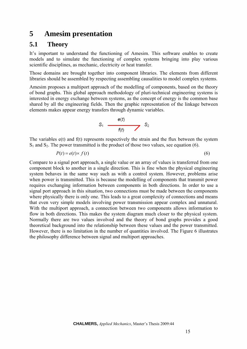
Amesim proposes a multiport approach of the modelling of components, based on the theory of bond graphs. This global approach methodology of pluri-technical engineering systems is interested in energy exchange between systems, as the concept of energy is the common base shared by all the engineering fields. Then the graphic representation of the linkage between elements makes appear energy transfers through dynamic variables.
The variables e(t) and f(t) represents respectively the strain and the flux between the system S1 and S2. The power transmitted is the product of those two values, see equation (6).
)()()( tftetP (6)
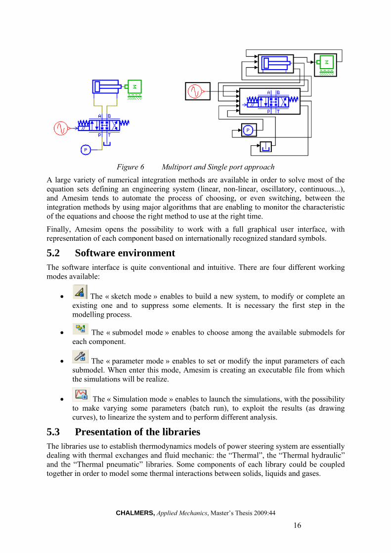
Compare to a signal port approach, a single value or an array of values is transferred from one component block to another in a single direction. This is fine when the physical engineering system behaves in the same way such as with a control system. However, problems arise when power is transmitted. This is because the modelling of components that transmit power requires exchanging information between components in both directions. In order to use a signal port approach in this situation, two connections must be made between the components where physically there is only one. This leads to a great complexity of connections and means that even very simple models involving power transmission appear complex and unnatural. With the multiport approach, a connection between two components allows information to flow in both directions. This makes the system diagram much closer to the physical system. Normally there are two values involved and the theory of bond graphs provides a good theoretical background into the relationship between these values and the power transmitted. However, there is no limitation in the number of quantities involved. The Figure 6 illustrates the philosophy difference between signal and multiport approaches.
CHALMERS, Applied Mechanics, Master’s Thesis 2009:44
16
Figure 6 Multiport and Single port approach
A large variety of numerical integration methods are available in order to solve most of the equation sets defining an engineering system (linear, non-linear, oscillatory, continuous...), and Amesim tends to automate the process of choosing, or even switching, between the integration methods by using major algorithms that are enabling to monitor the characteristic of the equations and choose the right method to use at the right time.
Finally, Amesim opens the possibility to work with a full graphical user interface, with representation of each component based on internationally recognized standard symbols.
5.2 Software environment The software interface is quite conventional and intuitive. There are four different working modes available:
The « sketch mode » enables to build a new system, to modify or complete an existing one and to suppress some elements. It is necessary the first step in the modelling process.
The « submodel mode » enables to choose among the available submodels for each component.
The « parameter mode » enables to set or modify the input parameters of each submodel. When enter this mode, Amesim is creating an executable file from which the simulations will be realize.
The « Simulation mode » enables to launch the simulations, with the possibility to make varying some parameters (batch run), to exploit the results (as drawing curves), to linearize the system and to perform different analysis.
5.3 Presentation of the libraries The libraries use to establish thermodynamics models of power steering system are essentially dealing with thermal exchanges and fluid mechanic: the “Thermal”, the “Thermal hydraulic” and the “Thermal pneumatic” libraries. Some components of each library could be coupled together in order to model some thermal interactions between solids, liquids and gases.

CHALMERS, Applied Mechanics, Master’s Thesis 2009:44
17
5.3.1 Thermal hydraulic library
The thermal-hydraulic library deals with liquids. It is based on a transient heat transfer approach. It is used to model thermal phenomena (energy transport, convection) and to study the temperature evolution in liquids when submitted to different kinds of heat sources. As a consequence thermal liquid properties are needed.
By using the thermal-hydraulic library it is also possible to model large thermal-hydraulic networks and evaluate pressure drops and mass flow rates through the components of these networks. The Figure 7 presents the main components available in the thermal hydraulic library.
Figure 7 Thermal hydraulic library
It is necessary to distinguish two types of components in the thermal-hydraulic library: The capacitive components are the volumes in which temperature and pressure are
calculated from the enthalpy and mass flow rates inputs at ports of these components. The submodel is based on the following statement: the energy stored in a thermal capacity induces a variation in the temperature of this capacity
The resistive components are the components in which the enthalpy and mass flow rates are evaluated from the temperature and pressure inputs at ports of these components. They are assumed to react instantaneously to the temperatures applied to them so that they are always in an equilibrium state.
That implies that a thermal-hydraulic model is always built with resistive components connected by capacitive components, see Figure 8.

CHALMERS, Applied Mechanics, Master’s Thesis 2009:44
18
Figure 8 Assembling causality
Three type of port can be encountered in the thermal hydraulic library:
The signal ports, input or output of a dimensionless value enabling the user to regulate or to measure parameters.
The thermal hydraulic ports that compute the values of temperature T(°C), enthalpy flow rate dmh(W), mass flow rate dm (kg/s) and pressure P (bar).
The thermal ports that exchange temperature T (°C) and heat flow rate dh (W).
Two kinds of calculations take place in the thermal hydraulic library: flow calculations and thermal calculations.
Flow calculation only occurs in resistive components. The evaluation of pressure drops and friction factors in every resistive component of the thermal-hydraulic library is based on Idel'cik (1986) formulation and assumptions. The fundamental relation used to evaluate the total pressure drop pΔ in a resistive component is based on Bernoulli's well-known equation.
2min
2
2 AQp
(7)
Where: Q: volumetric flow rate,
Amin: smallest cross-sectional area of the element considered. ζ: total friction factor; ρ: density of the fluid computed at mean pressure and upstream temperature
Every resistive component in the thermal-hydraulic library uses equation (7). This equation is manipulated so as to compute the volumetric flow rate from the pressure drop.
Then, thermal calculations take place both for resistive and capacitive components.
In capacitive components, the pressure and the temperature are computed from their derivatives with respect to time. These components can be considered as control volumes. The pressure is a state variable and is computed from the mass conservation assumption. In addition, the following assumption must be considered: in the control volume, the liquid properties are homogeneous. Using the definition of the liquid properties and more particularly the bulk modulus and the volumetric expansion coefficient, the pressure derivative with respect to time is given by:
dt
dT
dt
d
dt
dp..
1.

CHALMERS, Applied Mechanics, Master’s Thesis 2009:44
19
With:
p
Tp
),( , the isothermal fluid bulk modulus.
TTp
1),( , the volumetric expansion coefficient.
The temperature is a state variable and is computed from the energy conservation assumption. The temperature derivative with respect to time is given by:
dtdp
cT
cmQhdmdmhdmh
dtdT
pp
oi ...
Where m is the mass of liquid in the volume, cp is the specific heat of the liquid at constant pressure, dmhi is the incoming enthalpy flow rate, dmho is the outgoing enthalpy flow rate, Q is the heat flow exchanged with the outside, V is the volume, dm is the mass flow rate through the volume, α is the volumetric expansion coefficient, ρ is the fluid density and h is the specific enthalpy.
In resistive components, the mass flow rate and the enthalpy flow rates are computed. The mass flow rate is calculated from Bernoulli's equation. It is given by equation (8).
p
Acdm p
.2... (8)
The enthalpy flow rate is computed as follows:
hdmdmh
Where dm is the mass flow rate through the resistive component and h is the specific enthalpy of the fluid.
The thermal properties of the used fluid are required in order to allow flow and thermal calculations in the submodels of the thermal hydraulic library, especially the properties varying with respect to temperature and/or pressure (density, thermal capacity...).
5.3.2 Thermal library
The thermal library deals with solid materials. It is based on a transient heat transfer approach and is used to model traditional heat transfer modes, between solid materials. The submodels of the thermal library can be coupled with some other library.
There are two major types of submodels in the thermal library:
Submodels of heat transfer modes which do not have state variables (resistive submodels),
Submodels of thermal capacities, which have state variables (temperature and energy stored).
The Figure 9 presents the available submodels.

CHALMERS, Applied Mechanics, Master’s Thesis 2009:44
20
Figure 9 Thermal library
Thermal library components have thermal and signal ports. There are two variables exchanged at thermal ports
Temperature: T (degC),
Heat flow rate: dh (W).
These variables are available for plotting. As for the thermal hydraulic library, it’s necessary to respect an assembling causality: a thermal model is always built with resistive components connected by capacitive components.
The thermal capacity can be described as a temperature node. The temperature is computed from its derivative with respect to time and is considered to be homogeneous in the mass of solid involved. The temperature derivative is given by Equation (9).
p
outin
CmdtdT
(9)
Where Φin is the incoming heat flow rates (W); Φout the outgoing heat flow rates (W); m the mass of the considered solid; cp the specific heat.
The three types of heat transfer processes can be found: the conduction, the convection (free and forced) and the radiation. The two first phenomena have been described in the chapter 4.3 dealing with thermal exchanges. The submodels of the thermal library are following the physical mechanism and the equations stated.
In order to describe the temperature and heat flow rate evolution in the submodels of the library with respect to time, it’s necessary to have the thermal properties of the solid bringing into play.
5.3.3 Thermal pneumatic library
The last library used is the thermal pneumatic in order to take into account the convection phenomena between the exterior surfaces of the circuit’s components and the surrounding air. This library is similar to the thermal hydraulic, and the Figure 10 presents its submodels.

CHALMERS, Applied Mechanics, Master’s Thesis 2009:44
21
Figure 10 Thermal pneumatic library
It is based on a transient heat transfer approach and is used to model thermal phenomena in gases (energy transport, convection…) and to study the thermal evolution in those gases when submitted to different kinds of heat sources. As a consequence, special thermal gas properties are needed.
As for the previous libraries, the resistive components have to be linked together through capacitive components.
Thermal-pneumatic library components have Thermal-Pneumatic, Thermal and Signal ports.
Four variables are exchanged at Thermal-pneumatic ports:
Temperature: T (K),
Enthalpy flow rate: dmh (J/s)
Pressure: p (Pa),
Mass flow rate: dm (g/s).
Two variables are exchanged at thermal ports:
Temperature: T (degC),
Heat flow rate: dq (W).
These variables are available for plotting.
In the Thermal-pneumatic library, the gas used is assumed to be perfect or semi-perfect. The Thermal-pneumatic submodels are based on the perfect gas relation given by Equation (10).
TrmVP (10)
Where p is the absolute pressure (Pa), V is the volume (m3), m is the mass of gas (kg), r is the
gas constant (J/kg/K) and T is the temperature (K).
The submodels in the Thermal-pneumatic library use the first and second law of thermodynamics.

CHALMERS, Applied Mechanics, Master’s Thesis 2009:44
22
6 Development of a model The studied systems present an internal flow in a hydraulic circuit made up of oil pipes from different nature (rigid or flexible), diameter and length, and of active components such as the pump, the steering gear and the oil tank. This chapter presents how each element can be model on Amesim, with respect to the thermal exchanges and to the fluid mechanic, in order to reproduce the static tests of the validation procedure applied on each new circuit. The inputs needed to establish the model will be presented and their sensitivity and their control will be studied.
6.1 Modelling approach The development of a simulation tool has been done through the study of the theoretical thermal exchanges bringing into play for our problem and from the manipulation of Amesim by trying to model the physical phenomena identified. The development strategy has been turned around the study of two different existing circuits belonging to the vehicles Premium Lancer 8x4 LC MD11 and Premium T 4x2 MD11, both in left hand drive configuration.
The first one has been chosen because it’s representing historically the worst case of steering development ever encountered. In fact, twice in a row the engineers of Volvo 3P have been confronted to inacceptable results obtained during the validation tests. They have been struggling during months in order to find technical solutions to their overheating issue. As a consequence, this steering circuit benefits from many temperature acquisitions realized on different circuit configuration, with different cooling devices.
The second circuit has been chosen because of its radical difference with the first one, so that the modelling method could be correlated on two different kind of circuit.
A complete view of these circuits can be found in Appendix 4.
The objective of the thesis has been set to the validation of a model establishment method materialized by a utilization notice. The acquired knowledge on the subject is to be transmitted to Philippe Boitard, responsible for the design office calculations so that the modelling and the simulation culture could be introduced in the steering development process. This integration is planned step by step with a continuous refining of the representativeness of the model elements and a better control of the input parameters.
6.2 Characterization of materials and fluids
6.2.1 Presentation
To obtain realistic simulations of the thermal exchanges taking place around a power steering system and of the internal oil flow, it’s essential to accurately describe the physical and thermal properties of the materials and the fluids in presence.
The three thermal libraries used offer the possibility to define the thermal properties either for solids or fluids through special submodels, which have to be called in the components requiring the physical properties of the solid or the fluid they are made of or in contact with, in order to compute thermal or flow calculation.

CHALMERS, Applied Mechanics, Master’s Thesis 2009:44
23
Figure 12 Icon of thermal solid properties
The thermal library enables to describe the physical properties of the solid of a steering circuit with three special submodels associated to the icon presents by Figure 12.
THSD0: defining the thermal properties of solids by using second order polynomial function of the temperature,
THSD01: defining thermal properties of solids tanks to ASCII files,
THSD02: thermal properties defined by constants.
The Figure 13 shows the parameters to fill in order to define the properties of a material:
Figure 13 Parameters defining thermal solid properties
Those submodels share a common parameter: “the solid type index” parameter, which references the material. That index enables to link the material properties with the submodels that require them so as to compute flow and/or thermal calculations.
Then, the properties of different material are defined by inserting as many thermal solid properties submodel as necessary and taking care to assign different solid type index parameter to the solids to model, e.g. 1 for aluminium, 2 for steel, etc.... And for each submodel of the thermal library where a thermal property of a material is required to solve equations (density, specific heat or thermal conductivity) the user has to supply a solid type index.
An icon associated with submodel THSD0 added to the sketch of a system refers to one and only one material.

CHALMERS, Applied Mechanics, Master’s Thesis 2009:44
24
The “name of the solid” parameter is used especially if the user wants to cut off the system to model. In such two or more icons with the same thermal properties are added but with a different type index as well as a different name to each part.
The “filename for solid characteristic data” parameter is the file that must be supplied that contains all the data needed to compute the thermal properties of the solid. If the thermal properties are defined with constant with constant, then any file has to be supplied.
Amesim includes a material library referencing the most common used solid, as pure iron or aluminium, by using the THSD0 submodel.
THSD0 is used to set three main properties defining completely a solid from a thermal point of view. These three properties are the density, the specific heat and the thermal conductivity on which a temperature variation cannot be neglected. In the thermal library, those three quantities are defined by 2nd order polynomial functions of the temperature, see appendix 5.
Then thermal hydraulic submodels need to be supplied with the thermal properties of liquids in presence to compute the various variables exchanged at their ports. The thermal hydraulic library uses a special submodel named TFFD1 to handle the thermal properties of the liquids and to enable thermal and flow calculations. The Figure 14 shows the associated icon.
Figure 14 Icon for thermal hydraulic fluid properties
As solids, an “index of thermal hydraulic fluid” parameter is used to reference a liquid. That index is used to make the link between the thermal properties of a fluid and the submodels of the system, which require thermal properties to compute enthalpy flow rates, mass flow rates, pressures or temperatures.
The default index of hydraulic fluid is 1. Each icon associated with submodel TFFD1 inserted on the sketch of a system refers to one and only one liquid. If the considered system has more than one liquid, the corresponding number of icons must be added. Then a “filename for fluid characteristic data” has to be supplied. The file contains all the data needed to compute the thermal properties of the liquid used for a simulation. The thermal properties are varying with the temperature and/or pressure. The TFFD1 submodel is used to have access to four main properties completely defining a liquid with a thermal point of view. These four properties are the density, the absolute viscosity, the specific heat and the thermal conductivity. They are defined by 2nd order polynomial functions of temperature and pressure, see Appendix 6 for more details.
The thermal hydraulic library is provided with some predefined thermal properties of common liquids. Those files can be used directly in the TFFD1 submodel; they can be renamed and even modified for a given application. Moreover specific thermal liquid properties can be generated thanks to a special utility.
Finally the thermal properties of gases involved in the thermal exchanges of a steering circuit are needed in order to perform thermal calculations. The thermal pneumatic library proposes special submodels to handle those properties. The Figure 15 presents the icon associated.

CHALMERS, Applied Mechanics, Master’s Thesis 2009:44
25
Figure 15 Icon defining thermal pneumatic gas properties
Four submodels are associated with this icon: TPGD2, TPGD3 and TPGD4 define a perfect gas and TPGD1 an ideal or semi-perfect gas. As for the thermal and the thermal hydraulic libraries, some common gases are provided as customized submodels of the semi-perfect TPGD1 submodel. Semi-perfect gases are likely to follow the perfect gas relation (see equation 13)
In this submodel specific heat capacities are temperature dependant, and it’s considered as valid for medium pressure and significant temperature variations.
The parameter to fill in to define a semi-perfect gas are the same that those defining a liquid.
Submodels TPGDX are used to have access to four properties defining completely a gas: the constant-pressure specific heat, the perfect gas constant, the absolute viscosity and the thermal conductivity. If the gas is assumed to be perfect, theses properties are constant, while they will vary with temperature if the gas is assumed to be semi-perfect or ideal. In the Thermal-pneumatic library, these four quantities are defined by 2ndorder polynomial functions of the temperature; see Appendix 7 for more details.
6.2.2 Choice of the submodels
6.2.2.1 The Piping and the steering gear
On the occasion of the modelling of the steering circuit, the solid properties that have to be described are those of the constituent materials of the pipes and of the steering gear.
The influence of the thermal inertia of the piping is neglected: the mass of each pipe is set to 0.1 Kg. Then the thermal description of the pipe’s materials allows some approximation.
The steel pipes are made of TU37b shade. The associated submodel is a THSD0 type and a polynomial description of the stainless steel AISI 302, available in the thermal library, is chosen as parameter as shown in the Figure 16.
Figure 16 Definition of rigid pipes’ material

CHALMERS, Applied Mechanics, Master’s Thesis 2009:44
26
The flexible pipes of the steering circuits are made in synthetic rubber as the BNR (Nitrile butadiene rubber) or the CSM (Chlorosulfonated polyethylene). Those materials are modelled by a common submodel of the THSD02 type, which describes the thermal properties of rubber with constants as shown in the Figure 17.
Figure 17 Definition of flexible pipes’ material
Then the material of the steering gear needs to be thoroughly defined. In fact the mass of the steering gears varies between 40 and 50 kg, thus the thermal inertia of those components needs to be taken into account in the modelling. A thermal description of the material as accurate as possible is required. Following contacts with the steering gears suppliers, ZF and TRW, the materials have been defined as an homogenous cast alloy with constant thermal properties, as the range of temperature at which the steering gears are subjected is pretty small (for a metal). According to the suppliers, the material of these components is model by a THSD02 submodel of the thermal library shown in the Figure 18.
CHALMERS, Applied Mechanics, Master’s Thesis 2009:44
27
Figure 18 Definition of steering gears material
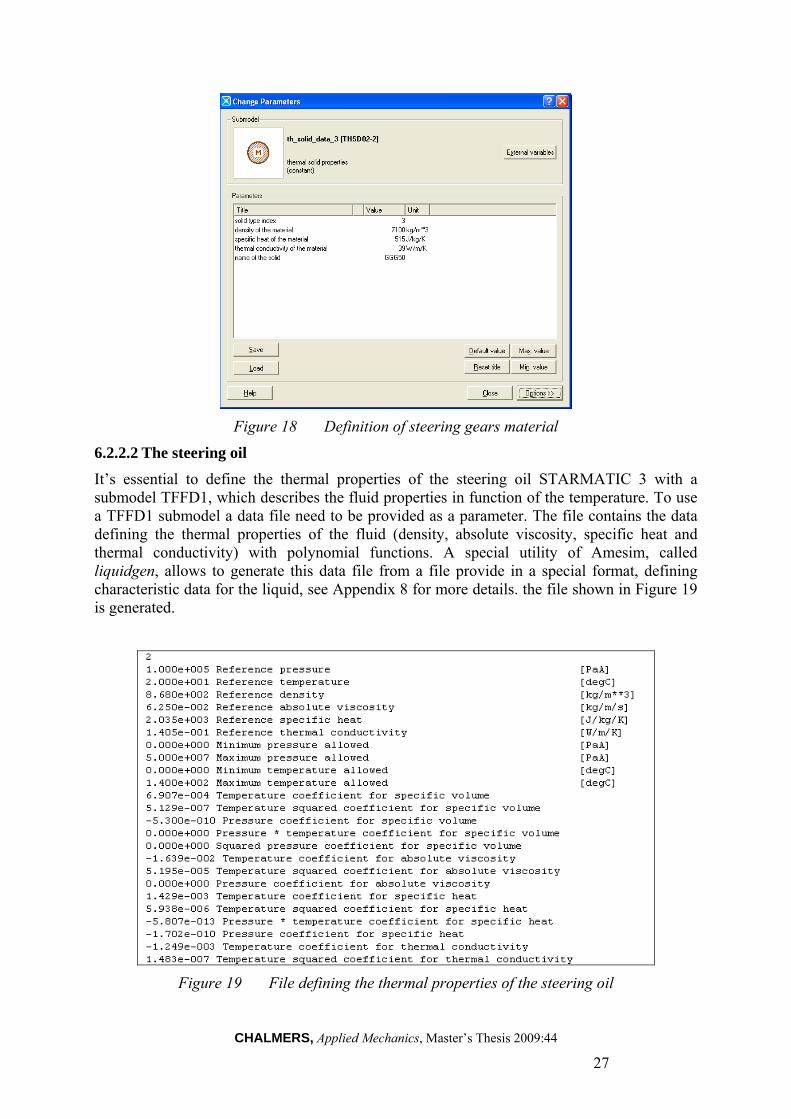
6.2.2.2 The steering oil
It’s essential to define the thermal properties of the steering oil STARMATIC 3 with a submodel TFFD1, which describes the fluid properties in function of the temperature. To use a TFFD1 submodel a data file need to be provided as a parameter. The file contains the data defining the thermal properties of the fluid (density, absolute viscosity, specific heat and thermal conductivity) with polynomial functions. A special utility of Amesim, called liquidgen, allows to generate this data file from a file provide in a special format, defining characteristic data for the liquid, see Appendix 8 for more details. the file shown in Figure 19 is generated.
Figure 19 File defining the thermal properties of the steering oil
CHALMERS, Applied Mechanics, Master’s Thesis 2009:44
28
Finally that file is attached to the “filename for characteristic data” parameter of the TFFD1 submodel used to define the thermal properties of the steering oil, as shown in Figure 20.
Figure 20 Definition of the steering oil properties
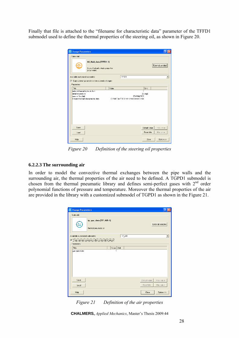
6.2.2.3 The surrounding air
In order to model the convective thermal exchanges between the pipe walls and the surrounding air, the thermal properties of the air need to be defined. A TGPD1 submodel is chosen from the thermal pneumatic library and defines semi-perfect gases with 2nd order polynomial functions of pressure and temperature. Moreover the thermal properties of the air are provided in the library with a customized submodel of TGPD1 as shown in the Figure 21.
Figure 21 Definition of the air properties

CHALMERS, Applied Mechanics, Master’s Thesis 2009:44
29
External convection, free
Oil (Toil,Poil,q)
6.3 The piping
6.3.1 Theory of thermal exchanges
The thermal exchanges between the steering oil and the surrounding air are function of the temperature gradient between those fluids. In fact, in one hand that gradient determines the direction of the heat flux in function that the surrounding is hotter than the oil or the opposite. In the other hand the more the temperature gradient is important, the more important the quantity of heat exchanged is. Nevertheless the temperature of the steering oil is inclined to rise in functioning. In that case the calories are exchanged from the oil to the surrounding air and all the pipes of the circuit become heat exchangers and allow the decreasing of the oil temperature.
Between the interior walls of the pipe and the steering oil occurs a forced convection: the oil yields some calorie to the cooler walls. The heat is then conducted along the pipe thickness from the interior to the exterior pipe walls. Finally the heat exchange process is completed by a free convective heat exchange between the exterior walls and the surrounding air. The air near the walls is warmed up, as a consequence its density proportionally decreases, it takes away the calories exchanged with the walls and it is replaced by some cooler surrounding air. That new air exchanges again with the heat source and the process goes on. Thus the temperature gradient between the surrounding air and the exterior pipe walls creates naturally a bulk air movement around the pipes. The Figure 22 illustrates the propagation of the heat flux between the steering oil and the surrounding air.
Figure 22 Heat exchange process for a pipe
Internal convection, forced
Conduction Air (Tair, P0)
Wall

CHALMERS, Applied Mechanics, Master’s Thesis 2009:44
30
Toil Tair
Forced convection
Free convection
Conduction
Tinternal_wall Texternal_wall
ii Sh 1
ee Sh 1
i
e
R
R
Lln
2
1
If the surrounding air is hotter than the oil, the calorie exchanges are done in the opposite direction.
The heat exchange process happens in series, as presents in the Figure 23. An analogy of that exchange mechanism with an electric system is possible. The temperature is equivalent to the voltage and the heat flux to the current. Then the expression of a thermal resistance function of the type of heat exchange (conductive, convective, radiative...) is deduced.
Figure 23 Modelling of the heat exchange process for a pipe
Where, hi: internal convective exchange coefficient,
Si: internal surface,
he: external convective exchange coefficient,
Se: external surface,
λ: Thermal conductivity of the material,
L: length of the pipe,
Ri: internal radius of the pipe,
Re: external radius of the pipe.
Then the equivalent thermal resistance of the exchange is equal to equation (11).
Toil Tair 1
hi Si
1
2 L ln
Re
Ri
1
he Se
i.e KS (Toil Tair )
With KS 1
1
hi Si
1
2 L ln
Re
Ri
1
he Se
(11)
It can be noticed that the thermal flux propagating from the steering oil to the surrounding air is constant along the process:
CHALMERS, Applied Mechanics, Master’s Thesis 2009:44
31
hi Si (Toil Tint_ wall ) 2 (Tmean ) L
ln(dext
dint
) (Tint_ wall Text _ wall ) he Se (Text _ wall Tair)
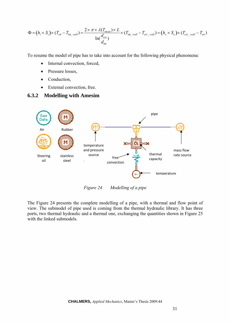
To resume the model of pipe has to take into account for the following physical phenomena:
Internal convection, forced,
Pressure losses,
Conduction,
External convection, free.
6.3.2 Modelling with Amesim
Figure 24 Modelling of a pipe
The Figure 24 presents the complete modelling of a pipe, with a thermal and flow point of view. The submodel of pipe used is coming from the thermal hydraulic library. It has three ports, two thermal hydraulic and a thermal one, exchanging the quantities shown in Figure 25 with the linked submodels.
Rubber
Steering oil
stainless steel
mass flow rate source
temperature and pressure
source
pipe
thermalcapacity free
convection
temperature
Air

CHALMERS, Applied Mechanics, Master’s Thesis 2009:44
32
Figure 25 Variables exchanged at pipe submodel ports
That submodel allows computing the pressure losses generated by the flowing of the steering oil in the pipe itself and the thermal exchanges induced by the internal forced convection between the interior pipe walls and the oil. The quantity of heat received by the interior pipe walls is then conducted along the pipe thickness.
The pressure losses are computed as equation (12).
²2
²
A
Q
D
lP
h
(12)
With: l: pipe length,
Dh: hydraulic diameter,
λ: friction factor.
And hD
l represents the global friction factor. The friction factor λ is depending on the
flow type: laminar or turbulent. In laminar regime, it is function of the Reynolds number Re , whereas in turbulent regime it depends of the relative roughness of the pipe
rrRe, , which explains hence the significant increase of the resistance to the displacement when the flow becomes turbulent.
The heat flux generated at the second port is computed as equation 13.
)( 23 TTAhQ conv (13)
Where, A: internal surface of the pipe (m²),
T2: temperature at port 2 (K),
T3: temperature at port 3 (K),
hconv: convective exchange coefficient (W/m²/K).
And
D
Nuhconv
PrRe
The parameters to fill in order to define the pipe submodel so as to perform thermal and flow calculations are its geometrical characteristics: diameter, length, cross-sectional area and thickness, and the young modulus of the material.

CHALMERS, Applied Mechanics, Master’s Thesis 2009:44
33
Then, a thermal capacity is placed between the submodel of pipe and the submodel of free convection. As previously stated it’s necessary to respect the alternation causality between resistive and capacitive submodels. The variables available at the ports of that submodel are shown in Figure 26.
Figure 26 Variables exchanged at thermal capacity ports
Null thermal heat sources are positioned at the ports 2 and 4, while at the ports 1 and 3 the heat flux circulates from the thermal port of the pipe until the free convection submodel. Each port computes the temperature of the capacity, considered as homogenous.
The only parameter to fill in order to define this component is the weight, which will systematically be taken at 0.1 Kg for all the piping element.
Finally a submodel of free convection is placed above the thermal capacity and allows modelling an external flow of natural convection between the pipe walls and the surrounding air. That submodel has two thermal ports as shown in Figure 27.
Figure 27 Variables exchanged at a free convection submodel ports
The state variables, T1 and T2, enable to compute the heat flow dh1 and dh2, which are equal but have opposite sign, according to equation (14).
)12(21 TTceareahdhdh conv (14)
The temperature T1 is set through a temperature source, which represents the temperature of the surrounding air around the considered pipe, and which depends on the zone where the pipe is placed.
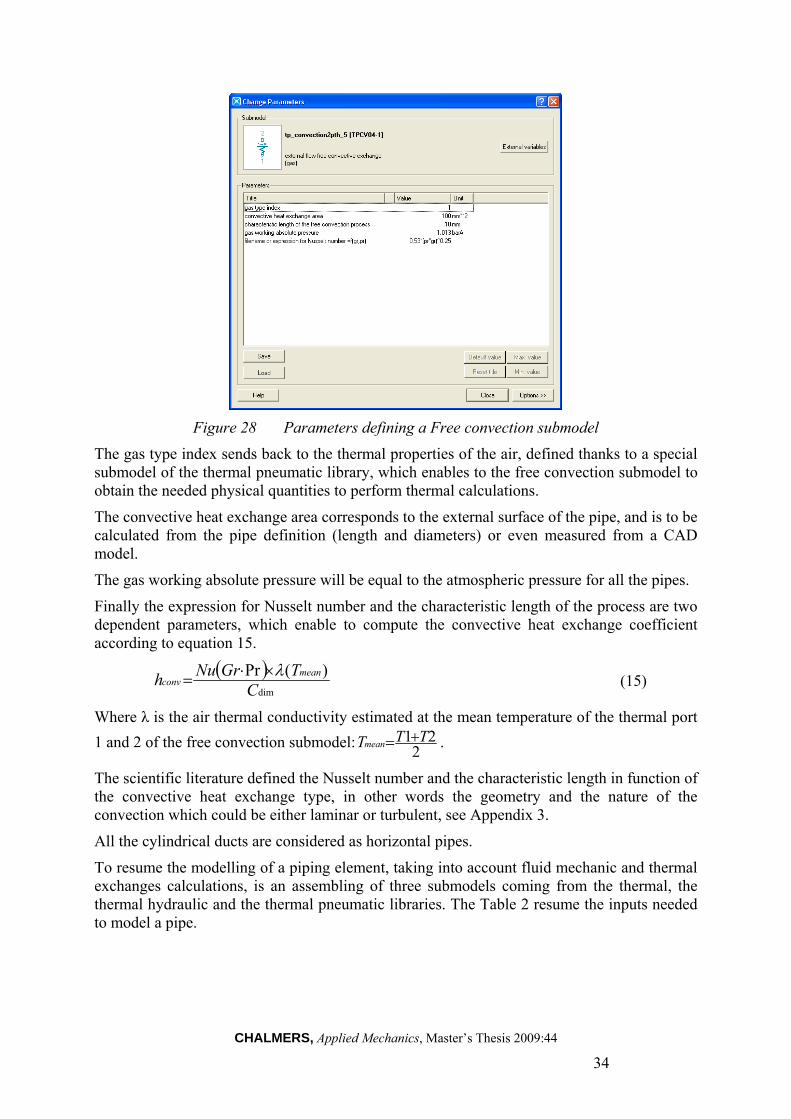
The user has to fill in the parameters presented in Figure 28 to define that submodel of the thermal pneumatic library:
CHALMERS, Applied Mechanics, Master’s Thesis 2009:44
34
Figure 28 Parameters defining a Free convection submodel
The gas type index sends back to the thermal properties of the air, defined thanks to a special submodel of the thermal pneumatic library, which enables to the free convection submodel to obtain the needed physical quantities to perform thermal calculations.
The convective heat exchange area corresponds to the external surface of the pipe, and is to be calculated from the pipe definition (length and diameters) or even measured from a CAD model.
The gas working absolute pressure will be equal to the atmospheric pressure for all the pipes.
Finally the expression for Nusselt number and the characteristic length of the process are two dependent parameters, which enable to compute the convective heat exchange coefficient according to equation 15.
dim
)(PrC
TGrNuh
meanconv
(15)
Where λ is the air thermal conductivity estimated at the mean temperature of the thermal port
1 and 2 of the free convection submodel:2
21 TTTmean .
The scientific literature defined the Nusselt number and the characteristic length in function of the convective heat exchange type, in other words the geometry and the nature of the convection which could be either laminar or turbulent, see Appendix 3.
All the cylindrical ducts are considered as horizontal pipes.
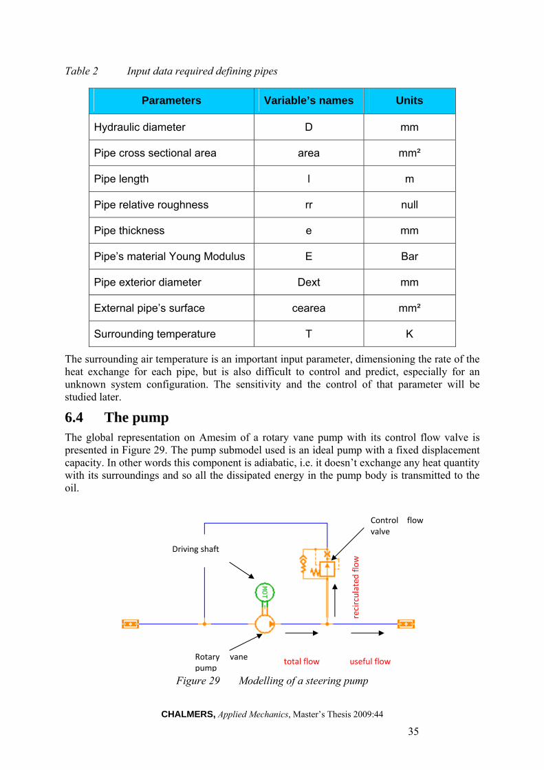
To resume the modelling of a piping element, taking into account fluid mechanic and thermal exchanges calculations, is an assembling of three submodels coming from the thermal, the thermal hydraulic and the thermal pneumatic libraries. The Table 2 resume the inputs needed to model a pipe.
CHALMERS, Applied Mechanics, Master’s Thesis 2009:44
35
Table 2 Input data required defining pipes
Parameters Variable’s names Units
Hydraulic diameter D mm
Pipe cross sectional area area mm²
Pipe length l m
Pipe relative roughness rr null
Pipe thickness e mm
Pipe’s material Young Modulus E Bar
Pipe exterior diameter Dext mm
External pipe’s surface cearea mm²
Surrounding temperature T K
The surrounding air temperature is an important input parameter, dimensioning the rate of the heat exchange for each pipe, but is also difficult to control and predict, especially for an unknown system configuration. The sensitivity and the control of that parameter will be studied later.
6.4 The pump The global representation on Amesim of a rotary vane pump with its control flow valve is presented in Figure 29. The pump submodel used is an ideal pump with a fixed displacement capacity. In other words this component is adiabatic, i.e. it doesn’t exchange any heat quantity with its surroundings and so all the dissipated energy in the pump body is transmitted to the oil.
Figure 29 Modelling of a steering pump
Rotary vane pump
useful flow total flow
recirculated flow Driving shaft
Control flow valve

CHALMERS, Applied Mechanics, Master’s Thesis 2009:44
36
Orifice
The flow rate delivered to the circuit is function of the pump capacity, the shaft speed and the suction pressure (at port 1). The only parameter defining the pump is its capacity.
The fluid flowing through the pump receives the energy stated by equation (16).
QPP )( 12 (16)
A shaft drives the pump in direct link. To simulate a static test, its rotational speed is set at a constant value, which corresponds to the engine speed multiplied by the gear ratio of the link between the crankshaft and the pump’s gear.
Finally the last component used to model the steering pump is a control flow valve. That submodel accepts a circulation of the fluid in both direction, and is made up of an orifice and a pressure relief valve. The variables exchanged at the ports of the submodel are presented in the Figure (30).
Figure 30 Variables exchanged at control flow valve submodel ports
The delivered flow rate is depending on the pressure difference across the valve and on the set parameter defining the orifice and the pressure relief valve. The functioning of that component is explained into details in Appendix 9.
The only parameter that has to be calculated is the set flow, which corresponds to the difference between the total flow rate delivered by the steering pump and the useful flow rate required by the power steering system. The table 3 presents an example of recirculated flow calculation for a given configuration in order to highlight the required inputs data to establish a pump model.
Table 3 Computation of the recirculated flow
Pump recirculated flow calculation
Example
Engine speed (rpm) w1 1700
Gear ratio crankshaft/pump gear R 1,74
pump speed (rpm) w2 = w1x R 2958
pump capacity (cc/rev) c 21
total flow rate (l/min) q1 = w2 x c / 1000 62,118
useful flow rate (l/min) q2 25
recirculated flow rate (l/min) q3 = q1 - q2 37,118
Pressure relief valve

CHALMERS, Applied Mechanics, Master’s Thesis 2009:44
37
The table 4 summarizes the input data required to model a steering pump in order to simulate a static test on a power steering system.
Table 4 Input data required defining a steering pump
Parameters Variables Units
Engine speed ω rev/min
Gear ratio crankshaft/pump gear R null
Pump capacity displ cc
Useful flow rate q L/min
6.5 The steering gear
6.4.1 Functioning
In static condition, without any steering wheel solicitation, the steering gear doesn’t provide any hydraulic assistance (See ¶ 4.2). In fact, the steering oil isn’t preferentially distributed in a cylinder chamber, as the control valve is in a neutral position, i.e. the inlet poppet and the ball screw nut are synchronized thanks to the torsion bar which is not solicited.
The oil flows from the pump to the central groove of the poppet, then passes through the inlet valves, between the socket and the poppet, towards both cylinder chambers, then reaches the radial grooves of the socket, and supplies the chambers of the cylinder which stays in its position. Finally the steering oil flows through the back groove of the socket and returns to the oil tank.
The flowing of the steering oil through axial and radial grooves, and along the circulation threads of the ball screw nut, implies the emergence of important pressure losses generated by the friction of the flow passing through hydraulic section of extremely narrow diameter (≤ 5 mm).
Moreover the mass of the component, which is assimilated to a casted piece, is significant which is conferring to the steering gear an important thermal inertia and the ability to stock heat.
Finally the external surfaces in contact with the surrounding air are a favourable field to convective thermal exchanges.
6.4.2 The steering gear modelling
To obtain accurate simulations of static tests on a power steering system, the physical consequences of the oil flow through the steering gear and the thermal exchanges with its surrounding have to be taken into account:
Important pressure drop between input/output of the steering gear,
Oil heating due to friction,
Internal forced convection,

CHALMERS, Applied Mechanics, Master’s Thesis 2009:44
38
Thermal inertia of the assemble,
Free convection between the steering gear walls and the surrounding air.
A closed collaboration with the steering gear suppliers has led to establish the needed input data to model those physical phenomena. A characterisation of each steering gear is done by the suppliers in order to define the pressure drop encountered at a given flow rate and steering oil temperature. The mass of the steering gear and the thermal properties of the used material, as well as its oil capacity are also data to be provided by the suppliers.
The hydraulic path follow by the oil within the component is an important parameter to be defined in order to obtain the right thermal exchanges by forced convection and the right amount of friction with the corresponding pressure losses. Unfortunately that parameter could not be defined in an easy way, and has been approximated.
Finally the thermal exchanges by free convection are to be defined with the external surfaces of the steering gear, which could be directly measured on the CAD models, and with the expression of a Nusselt number and a characteristic length. As the geometry of the component is quite complex any Nusselt correlation could be used. A given value for the convective exchange coefficient will be aimed at. The Figure 31 presents the steering gear model.
Figure 31 Modelling of a steering gear
Three elements are used to model the steering gear:
A thermal orifice modelling the pressure drop across the steering gear,
An hydraulic capacity receiving a thermal flux corresponding to the pressure drop across the orifice,
A pipe section with thermal exchange and without friction, representing the hydraulic path of the steering oil with a forced convection, and exchanging with the surrounding air by free convection through a thermal capacity representing the steering gear mass.
air
steering oil
GGG50
Thermal orifice
Thermal hydraulic capacity
Heat flux source
Hydraulic path

CHALMERS, Applied Mechanics, Master’s Thesis 2009:44
39
The thermal orifice is characterized by a pressure drop at a given flow rate, here the useful flow of the circuit. Temperature and pressure are the input data used at the component ports in order to determine the flow rate and the enthalpy flux.
Then, the heat flux received by the fluid flowing through the steering gear corresponds to the product of the pressure drop across the valve with the flow rate, see equation (16).
The pressure P1 and P2 are measured around the orifice with pressure sensors, and the heat flux is supplied to the fluid with a heat flux source place on a thermal hydraulic capacity.
That capacity represents the oil capacity of the steering gear, data provided by the suppliers. The only parameters to fill in to define that component are the index of thermal hydraulic fluid flowing inside and its volume. The volume of the capacity hasn’t any influence on the final result of the simulation, i.e. the final temperature, but only on the dynamic of the model. The more important the volume is the more the uprising kinetic of temperature is slow.
The last elements defining the steering gear consider the thermal exchanges between the oil and the surrounding air. There are a submodel of thermal hydraulic pipe, TFPC5, with thermal exchanges and without friction, a submodel of thermal capacity and a submodel of free convection. The set pipe represents the hydraulic path within the steering gear in static condition. The Figure 32 shows the parameters to fill in to define the pipe.
Figure 32 Parameters defining the pipe submodel for the steering gear
The diameter and the length of the section are set in function of the steering gear type. Unfortunately the steering gear suppliers, ZF and TRW, haven’t be able to provide any data concerning the hydraulic path, however according to “front and rear axle installation” design office members, an hydraulic diameter of 5mm and a length included within the range 0.1 m≤ l ≤ 0.3 m have been defined for the modelling of the steering gears.
The internal convective exchange coefficient, hi, is evaluated from tests realized on a thermal hydraulic pipe TFPC05, where this parameter appears as an internal variable, at which is assigned the same geometrical parameters. Then the measured value of the parameter is carried forward in the TFPC5 thermal pipe submodel used for the steering gear modelling.

CHALMERS, Applied Mechanics, Master’s Thesis 2009:44
40
The submodel defining the free convective exchange process is the same as the one used for the piping element (see ¶ 6.3.2). As any empirical correlation cannot be used to define the Nusselt number (complex geometry) a target value will be aim at for the convective exchange coefficient. The characteristic length of the process is set. According to the literature and the Volvo 3P engineers experience, a common value of convective exchange coefficient between steel alloy walls and some air is around: he = 25 w/m²/K.
By stetting the characteristic length of the process at the width of the steering gear, the value of the Nusselt number is set in the free convection submodel according to equation (17).
Nu he Cdim
(Tmean ) (17)
The input data needed to model a steering gear to simulate a static test are summarized in Table 5.
Table 5 Input data required to a steering gear
Parameters variables
Units
Hydraulic diameter D mm
Pipe cross sectional area area mm²
Pipe length l m
Internal convective exchange coefficient
hi W/m²/K
Pipe thickness e mm
Material young modulus E Bar
Steering gear mass m Kg
Steering gear width w mm
Steering gear external surface cearea mm²
Surrounding air temperature T K

CHALMERS, Applied Mechanics, Master’s Thesis 2009:44
41
7 Presentation of models and simulations From the previous considerations on the modelling of the different components of a power steering system, complete steering circuit are built in order to perform thermal and flow calculations to evaluate the stabilized temperature of the steering oil when simulating a static test.
7.1 Introduction To establish a complete model of a power steering system to perform static test simulations, all the required components of the three thermal libraries need to be gathered:
Piping and oil tank,
Steering pump,
Steering gear.
This step is done in the sketch mode of Amesim.
Then the parameters of those submodels need to be set so as to perform simulations reproducing the static tests in place at Volvo 3P. This step is done in the parameter mode of Amesim. The most sensible parameter to set is the surrounding air temperature, as that parameter is to be set for all the piping elements and the steering gear, and it is defining the quantity of calorie exchange between the steering oil flowing through these elements and the surrounding air.
Its value depends on various factor as the type of engine used, the position of the considered element, the engine speed at which the static test is performed or the presence or not of phonic insulation panels around the circuit. The influence of those factors is difficult to grasp and to control in order to predict the surrounding temperature around circuit components.
Nevertheless the important data base of temperature, coming from the temperature recording campaigns carried out on the previous vehicle generations enables to estimate the surrounding temperature in function of the truck’s zone where is situated the considered element. In fact the data acquisition box used during the static tests, are equipped of several tracks dedicated to the temperature recording (an example of data acquisition is given in appendix 10), and especially the surrounding temperature in different part of the trucks where the steering circuit is spread. For each kind of steering circuit it is possible to find the recordings of the surrounding temperature around the oil tank and of the external temperature in the engineering report of the validation procedure. Many more could be found as the surrounding temperature around the steering gear, or different coolant organ.
Finally to estimate the values of temperature to assign to the thermal sources of the free convective exchange submodels, the temperature records realized on similar vehicles should be considered. The models are cut off in different thermal zone. An example is shown in Figure 33 for a Premium 8x4 LC, at which the steering circuit is cut off on in four distinct thermal zones:

CHALMERS, Applied Mechanics, Master’s Thesis 2009:44
42
Figure 33 Example of circuit cuts in thermal zone
At the occasion of the thesis, a rapprochement between the calculations lead at the “front and rear axle installation” design office and the Computational Fluid Dynamics calculation unit of the design office ”Powertrain Installation” has begun. Their experience in the temperature forecasting calculations, dedicated to the design of heat exchangers for engine components, enables to consider the possibility to enhance the surrounding temperature predictions around the power steering system elements in order to increase the accuracy of the modelling.
The design office has to manipulate the input data of the model and realizes thermal simulation on power steering circuit in development as to gain in experience and enhance the control of the input, and especially the surrounding air temperatures.
7.2 Complete model example The Figure 34 presents an example of modelling of a complete power steering system coming from a Premium Lancer LC 8x4 MD 11 left hand drive. Seven temperature sensors are placed along the model, and the mean temperature is taken as reference at the end of the simulation:
oil tank
steering gear
cross beam
front side

CHALMERS, Applied Mechanics, Master’s Thesis 2009:44
43
Figure 34 Example of a complete steering model from the Premium 8x4 LC

CHALMERS, Applied Mechanics, Master’s Thesis 2009:44
44
7.3 Simulations
7.3.1 Simulation settings
The Amesim simulation mode is a numerical solver, which does successive iterations based on calculation algorithm. Various options, shown on Figure 35, are available to realize the simulation:
The type of integrator used, the standard one will be chosen,
The simulation length,
The step between each iteration.
Figure 35 Simulation settings
It’s also possible to study the influence of a specific parameter, by assigning it different chosen values, and then performing the simulations in a row.
When choosing the standard integrator, Amesim is performing a convergence test after each iteration, and if the result converges an error test is applied to check if the result is accurate enough. Both tests are using the same tolerance that is a parameter to be set. If one of the test failed the simulation is stopped, and it’s needed to set a smaller tolerance value. If different results are obtained by decreasing the tolerance, the one with the smallest value is to be trusted.
7.3.2 Data processing
When the simulation is finished, each submodel returns the values of the variables exchanged at their ports. A special utility, Ameplot, enables to visualise these results, to perform calculations and to compare some parameters configurations. The Figure 36 presents the variables available for consultation for an oil tank at the end of a simulation.

CHALMERS, Applied Mechanics, Master’s Thesis 2009:44
45
Figure 36 Consultation of computed variables at submodel ports
By default the variables are plotted with respect to time, but the plot manager enables to add as much data as needed and to manipulate them, for example to assign a variable at an axis or to perform calculation.
7.4 Presentation of results This chapter confronts the simulation results obtained from the model build on Amesim with results coming from the validation process of steering circuits. Two kinds of circuits are compared.
7.4.1 Premium Lancer LC 8x4 MD11 left hand drive
The power steering system of that vehicle has been subjected to an important test campaign in order to satisfy the steering oil temperature criteria acceptability. As the initial design was unacceptable in term of oil temperature levels reached, the engineers have modified the validation procedure and the circuit design. According to procedure, the maximum engine speed is to be used for the static test, i.e. 2200 rpm in the case on that vehicle. An investigation next to the commercial network has shown that in usage the engine speed would not excess 1700 rpm in static. So two engine speeds have been selected for the static test: 1700 rpm and 2100 rpm, and the first one is kept as acceptability criteria for the static test.
Then two circuits configuration have been tested, a first one with a single heat exchanger place in front side in front of the fan, and a second one with a double heat exchanger.
Finally four test configurations have been subjected to temperature recording, and they can be compared with the results obtained with the model established on Amesim, according to the component modelling method established. The Table 6 shown the confrontation of the results obtained in reality, on two prototype vehicle 911H and 912H, with the simulation results.

CHALMERS, Applied Mechanics, Master’s Thesis 2009:44
46
Table 6 Results comparing between simulations and testing, Premium 8x4 LC
Engine speed (rpm) Heat exchanger Steering oil
temperature(°C), after 5000s of simulation.
Steering oil temperature(°C) in
testing.
1700 single 135°C 130°C, under 25°C (911H)
129°C under 23°C (912H)
1700 double 131,5°C 129°C under 26°C (912H)
2100 single 143°C 137°C under 26°C (912H)
2100 double 139°C 133°C under 26°C (912H)
7.4.2 Premium 4x2 MD11 left hand drive
The Premium 4x2 MD11 vehicle has follow two measurement campaigns, one satisfying the euro4 regulation and the other one the euro5. A comparison of the steering oil temperature obtained in testing with the results provide by the corresponding simulation models has been led.
Two circuit configurations have been tested, both for euro4 and euro5, one with a serpentine, as a coolant device, one without. The Table 7 confronts the results obtained from the calculations with the physical testing.
Table 7 Results comparing between simulation and testing, Premium 4x2
Engine speed (rpm) Coolant device Steering oil temperature(°C) after 7200s of simulation
Steering oil temperature (°C) in testing
2100 serpentine 107°C
110°C under 23°C (euro5)
111°C under 18°C (euro4)
2100 null 114°C
122°C under 21°C (euro5)
117°C under 29°C (euro4)

CHALMERS, Applied Mechanics, Master’s Thesis 2009:44
47
8 Conclusion and recommendations 8.1 Conclusion The simulation tool of steering oil temperature prediction develop on Amesim has given interesting results on two completely different steering circuits. The physical phenomena influencing the oil temperature at the occasion of a static test are identified and their modelling has shown encouraging results. Unfortunately the models have not been confronted to the reality due to the financial crisis. The tests initially plan during the period of the thesis have been delayed. The next step to strengthen the modelling method is to compare its performances with the reality. Nevertheless the design office “Front and Rear axle installation” benefits of a solid base to introduce the simulation in the development process of the steering circuit so as to size them properly and design the right function at the right time and the right cost. In fact the obtained results show that an overheating issue is predictable. But the accuracy of the model cannot be fully trusted until a comparison with testing.
8.2 Recommendations
8.2.1 Characterisation of the steering gear
The hydraulic path of the steering gear in terms of length and diameter is not properly defined. As a consequence, the thermal exchanges between the steering oil and the surrounding air have been approximated, notably through the convective exchange coefficient between the oil and the internal wall of the steering gear. This parameter is an input data to provide for the steering gear modelling, and is sizing the quantity of heat exchange with the surrounding. In fact, the heat flux gives off from the fluid towards the internal steering gear walls is given by equation (18):
(hi Si) (Toil Tint_ wall ) (18)
Then an accurate definition, either of the hydraulic path or of the thermal exchanges, would be desirable for each steering gear for a total control of their role in the evacuation of calories.
To reach that goal, partnership with the components’ suppliers should be considered. To establish a characterization procedure of the thermal exchanges is also a possibility.
8.2.2 Surrounding temperature control
The surrounding air temperatures are some sensitive input data in the steering models. In fact a variation of all the temperature set from the same amount is identically reflected on the temperature reached by the steering at the end of a simulation.
Moreover, it has been noticed during the static test that the starting of the fan, at which the strategy is managed for the engine components, is strongly influencing the surrounding temperature as well as the steering oil temperature itself. In fact the cyclic occurrence of a forced flow around the circuit’s pipes induces a cyclic alternation between forced and free convective heat exchange process, knowing that the quantity of calories exchanged is much higher in a forced convection process. So the considering of the fan strategy could be a way to enhance the accuracy of the models in the future.

CHALMERS, Applied Mechanics, Master’s Thesis 2009:44
48
9 References Incropera, DeWitt (2006): Fundamentals of Heat and Mass Transfer, 5th Edition
M.VergéD.Jaume (2003): Modélisationstructurée des systèmes avec les Bond Graphs
I.Idel’cik (1986): Mémento des pertes de charges
Bosch (2004): Automotive Handbook, 6th Edition

CHALMERS, Applied Mechanics, Master’s Thesis 2009:44
49
Appendix 1 Conduction heat transfer Contact conduction:
The heat flux propagating through two solids in contact is expressed by:
TGA
Where A: contact exchange surface (m²)
G: conductance of the contact, function of the surfaces roughness (W/m²/K)
Linear conduction:
Through a given material, the heat flux flowing linearly is equal to:
Td
ATmean )(
Where, λ: Thermal conductivity of the material (w/m/K)
A: Exchange surface (m²)
d: Distance between the considered points (m)
Thermal conductivity of the material is depending on the temperature and is taken at the
average temperature between the two nodes of the studied element: 2
)( 21 TTTmean
Cylindrical conduction:
The heat flow propagating through the wall of a cylinder is expressed as:
T
dd
LText
mean
intln
)(2
With L: Cylinder length (m)
dext: Exterior diameter (m)
dint: Interior diameter (m)
General case:
The general expression of heat flux flowing through a solid subjected to a temperature gradient at its ends is expressed by:
TST fmean )(
Sf is the form factor concerning the geometrical configuration (expressed in meter), and )( meanT the average thermal conductivity between the solid ends (W/m/K).

CHALMERS, Applied Mechanics, Master’s Thesis 2009:44
50
Appendix 2 The Dimensionless numbers The Prandlt number is expressed as:
CpPr
With, µ: absolute viscosity of the fluid (Pa.s),
λ: thermal conductivity of the fluid (W/m/K)
Cp: thermal capacity of the fluid (J/K/kg)
This dimensionless quantity represents the ratio of the momentum diffusivity and the thermal diffusivity.
The Reynolds number is equal to:
DV Re
With, V: flow velocity (m/s)
D: hydraulic diameter (m)
ν: Kinematic viscosity (m²/s)
The Reynolds number gives a measure of the ratio of the inertial forces to viscous forces. It characterizes the flow regime, either laminar or turbulent. Laminar flow occurs at low Reynolds number, and is defined by a smooth flow at slow motion, while turbulent flow occurs at high Reynolds number and tends to create random eddies, vortices and other flow fluctuation. The critical Reynolds number marks the limit between those two domains.
The Grashof number is the ratio of buoyancy force and viscous forces:
2
3
dim
surfacefluide TTgC
Gr
With, β: the volume expansivity (K-1),
g: acceleration due to gravity (m.s-2),
ΔT: temperature difference between hot surface and bulk fluid (K),
Cdim: characteristic length (m), and ν is the viscosity.
Those dimensionless number involved in the calculation of the convective exchange coefficient, are referring to the fundamentals physics properties of the convected fluid taken at
the mean temperature of the exchange between the wall and the fluid: 2
wallfluidmean
TTT

CHALMERS, Applied Mechanics, Master’s Thesis 2009:44
51
Appendix 3 Nusselt Correlations The following chart details the most common Nusselt correlation for forced convective heat transfer, caused by an external flow, in function of the geometry and of the flow type:
The following chart summarizes the usual Nusselt correlations for forced convective heat transfer coming from an internal flow in a cylindrical conduct, in function of the flow type:
Finally, the general form of the Nusselt number for free convective heat transfer is: nGrCNu Pr)( . The following chart details the assigned values to the C and n coefficient
in function of the geometric configuration and of the flow type:

CHALMERS, Applied Mechanics, Master’s Thesis 2009:44
52
Appendix 4 Examples of circuit overview Here is a CAD model of the steering circuit coming from a Premium 4x2 MD11:
Here is an overview of a steering circuit of a Premium 8x4 LC MD11:

CHALMERS, Applied Mechanics, Master’s Thesis 2009:44
53
Appendix 5 Solid thermal properties Density ρ:
ρ = ρ0 x (1+ At x ΔT + At2 x ΔT2)
At and At2 are proper coefficient of the solid
ρ0: reference density at temperature reference (Tref)
ΔT = Tw– Tref, with Tw is the working temperature
Unit ρ: kg/m3
Specific heat Cp:
Cp = Cp0 x (1+ Bt x ΔT + Bt2 x ΔT 2)
Bt and Bt2 are proper coefficient of the solid
Cp0: reference specific heat at Tref
ΔT = Tw– Tref
Unit Cp: J/kg/K
Thermal conductivity λ:
λ�= λ0 x (1+ Ct x ΔT + Ct2 x ΔT 2)
Ct and Ct2 are proper coefficient of the solid
λ0 : reference thermal conductivity at Tref
ΔT = Tw– Tref
Unit λ: W/m/K
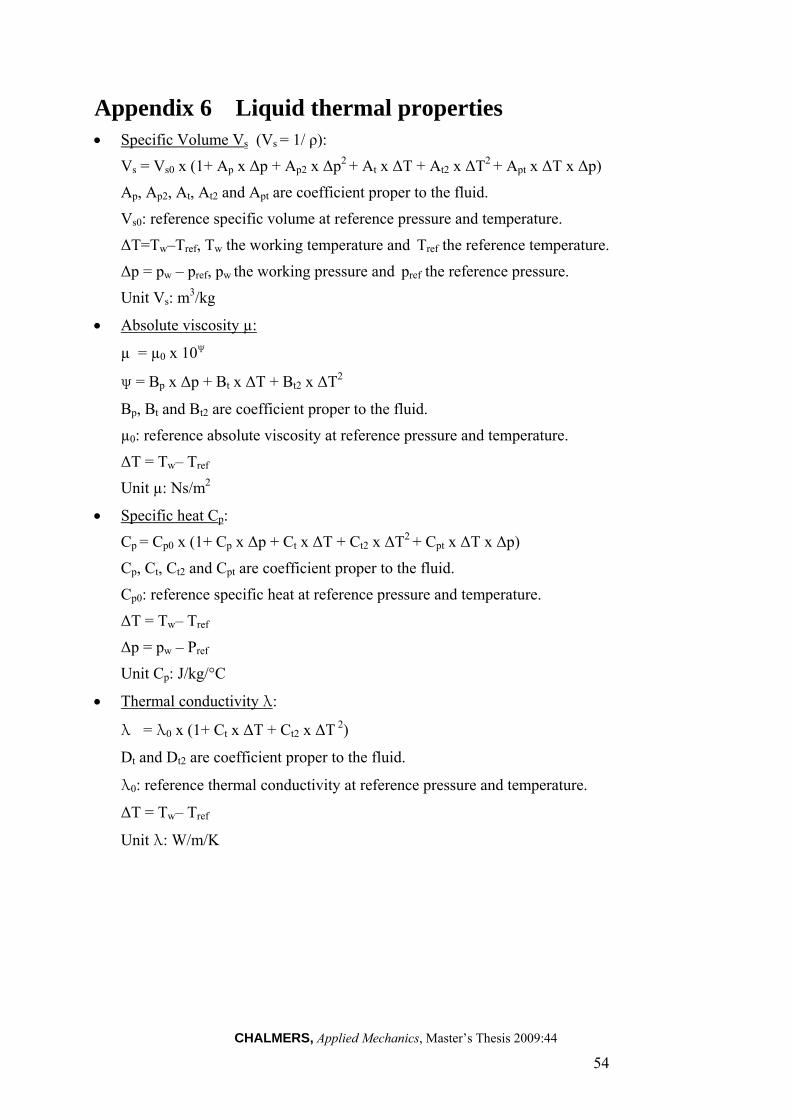
CHALMERS, Applied Mechanics, Master’s Thesis 2009:44
54
Appendix 6 Liquid thermal properties Specific Volume Vs (Vs = 1/ ρ):
Vs = Vs0 x (1+ Ap x Δp + Ap2 x Δp2 + At x ΔT + At2 x ΔT2 + Apt x ΔT x Δp)
Ap, Ap2, At, At2 and Apt are coefficient proper to the fluid.
Vs0: reference specific volume at reference pressure and temperature.
ΔT=Tw–Tref, Tw the working temperature and Tref the reference temperature.
Δp = pw – pref, pw the working pressure and pref the reference pressure.
Unit Vs: m3/kg
Absolute viscosity µ:
µ = µ0 x 10ψ
ψ = Bp x Δp + Bt x ΔT + Bt2 x ΔT2
Bp, Bt and Bt2 are coefficient proper to the fluid.
µ0: reference absolute viscosity at reference pressure and temperature.
ΔT = Tw– Tref
Unit µ: Ns/m2
Specific heat Cp:
Cp = Cp0 x (1+ Cp x Δp + Ct x ΔT + Ct2 x ΔT2 + Cpt x ΔT x Δp)
Cp, Ct, Ct2 and Cpt are coefficient proper to the fluid.
Cp0: reference specific heat at reference pressure and temperature.
ΔT = Tw– Tref
Δp = pw – Pref
Unit Cp: J/kg/°C
Thermal conductivity λ:
λ�= λ0 x (1+ Ct x ΔT + Ct2 x ΔT 2)
Dt and Dt2 are coefficient proper to the fluid.
λ0: reference thermal conductivity at reference pressure and temperature.
ΔT = Tw– Tref
Unit λ: W/m/K

CHALMERS, Applied Mechanics, Master’s Thesis 2009:44
55
Appendix 7 Gas thermal properties Absolute viscosity µ:
µ = µ0 x 10ψ
Where: ψ = ac + at x ΔT + at2 x (ΔT)²
ac, at and at2 are coefficients proper to the gas.
µ0: reference absolute viscosity at reference temperature and pressure.
ΔT = Tw– Tref
Unit µ: Kg/m/s
Constant pressure specific heat:
Cp = Cp0 x [ bc + bt x ΔT + bt2 x (ΔT)²]
bc, bt and bt2 are coefficients proper to the gas.
Cp0: reference constant pressure specific heat at temperature reference.
ΔT = Tw– Tref
Unit Cp: J/kg/K
Thermal conductivity:
λ�= λ0 x (cc + ct x ΔT + ct2 x ΔT 2)
cc, ct and ct2 are coefficients proper to the gas.
λ0: reference thermal conductivity at temperature and pressure reference
ΔT = Tw– Tref
Unit λ: W/m/K
Perfect gas constant:
ref
ref
T
Pr
0
Pref : pressure reference
Tref : temperature reference
ρ0: reference density at temperature and pressure reference
Unit r: J/kg/K

CHALMERS, Applied Mechanics, Master’s Thesis 2009:44
56
Appendix 8 Definition of the STARMATIC 3 oil To create the data file defining the steering oil thermal properties in function of 2nd order polynomial functions of temperature, four thermal properties of the liquid need to be provided at least at three temperature points. The more points are provided over the temperature range the more accurate the submodel will be. According to the Renault Trucks Oil department, three points defining those properties have been defined. Generating this type of file requires special attention. In addition, the fluids used in the system have to work in the defined range of temperature and pressure.
The data characteristic file built is:
The pressure coefficient for specific volume should never be equal to zero, and is equal to:
refrefp PT
a,
1
Where β(Tref,Pref) is the reference bulk modulus, given at reference pressure and temperature.

CHALMERS, Applied Mechanics, Master’s Thesis 2009:44
57
Appendix 9 Functioning of the control flow valve The following diagram presents the functioning mode of the control flow valve:
For a static test, the pressure drop across the valve would never be negative as the pressure at the pump output will always be higher than the input. So the pressure relief valve will stay closed.
The orifice has two functioning mode depending on the set parameters:
The cross sectional area of the orifice is function of the set flow qset defined at the minimum operating pressure difference Pmin. If the pressure difference across the valve, ΔP input/output, is contained within the range [0; Pmin], the flow rate crossing the valve is proportional to qset such as:
setqP
PPQ
min
12 )(
When the ΔP across the valve is higher than or equal to Pmin, the flow rate crossing the valve is equal to the set flow qset, compensated by the product of the ΔP with a flow rate pressure gradient such as:
gradPPqQ set )( 12
As a constant flow has to be simulated, the recirculated flow through the control flow valve needs to be as well constant. As a consequence a small minimum operating pressure difference will be chosen and a null flow rate pressure gradient, so that the control flow valve would always follow the second operating mode.

CHALMERS, Applied Mechanics, Master’s Thesis 2009:44
58
Appendix 10 Example of steering oil temperature measurement Measurement equipment: Recorder-Reader "Ecureuil 1200" GRANT N° RVI 344327U / AB000290 + 6 temperature sensors:
Track 1: Cab surrounding, Track 2: Steering oil in the oil tank N° 1, Track 3: Oil tank surrounding, Track 4: Serpentine surrounding, Track 5: Steering oil in the oil tank N° 2, Track 6: Rear vehicle.
Static measurement (interior) 1700 rpm:
Static measurement, 2100 rpm, with fan punctually:

CHALMERS, Applied Mechanics, Master’s Thesis 2009:44
59
Dynamic measurement, «MONTEE HUEZ» criteria: