Establishing RelationshipsLinear Least Squares Fitting

Lecture 6Physics 2CL

Summer 2010

Outline

• Determining the relationship between measured values

• Physics for experiment # 3 – Oscillations & resonance

• Overview of last set of three labs

ScheduleMeeting Experiment

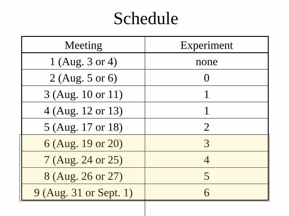
1 (Aug. 3 or 4) none2 (Aug. 5 or 6) 0

3 (Aug. 10 or 11) 14 (Aug. 12 or 13) 15 (Aug. 17 or 18) 26 (Aug. 19 or 20) 37 (Aug. 24 or 25) 48 (Aug. 26 or 27) 5

9 (Aug. 31 or Sept. 1) 6

Relationships

• So far, we’ve talked about measuring a single quantity

• Often experiments measure two variables, both varying simultaneously

• Want to know mathematical relationship between them

• Want to compare to models• How to analyze quantitatively?

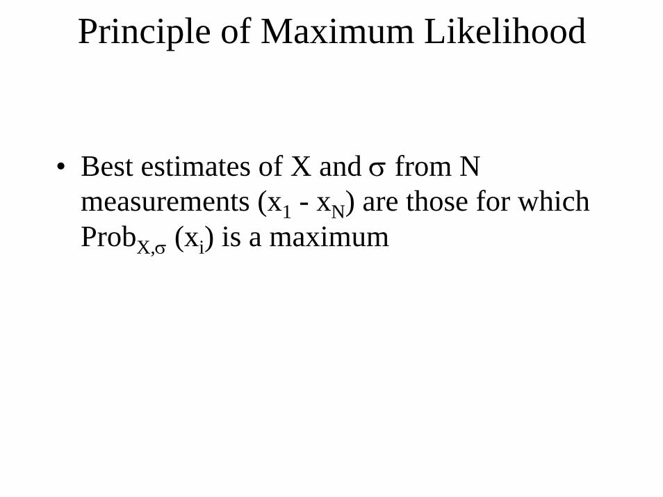
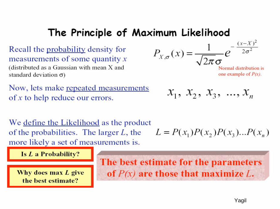
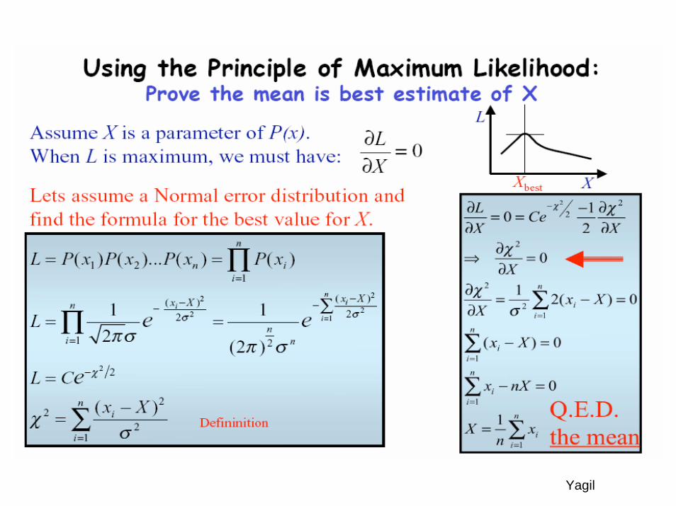
Principle of Maximum Likelihood

• Best estimates of X and σ from N measurements (x1 - xN) are those for which ProbX,σ (xi) is a maximum

Yagil

Yagil

Yagil

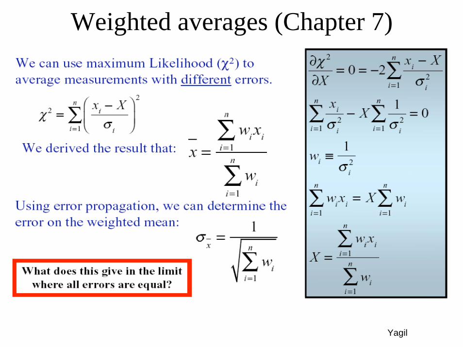
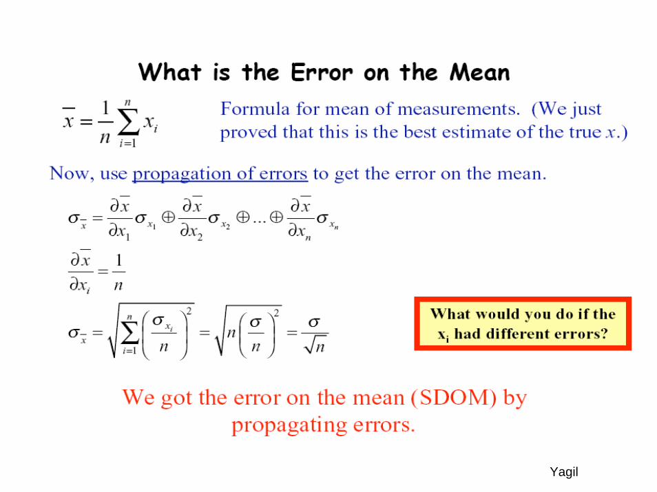
Weighted averages (Chapter 7)

Yagil

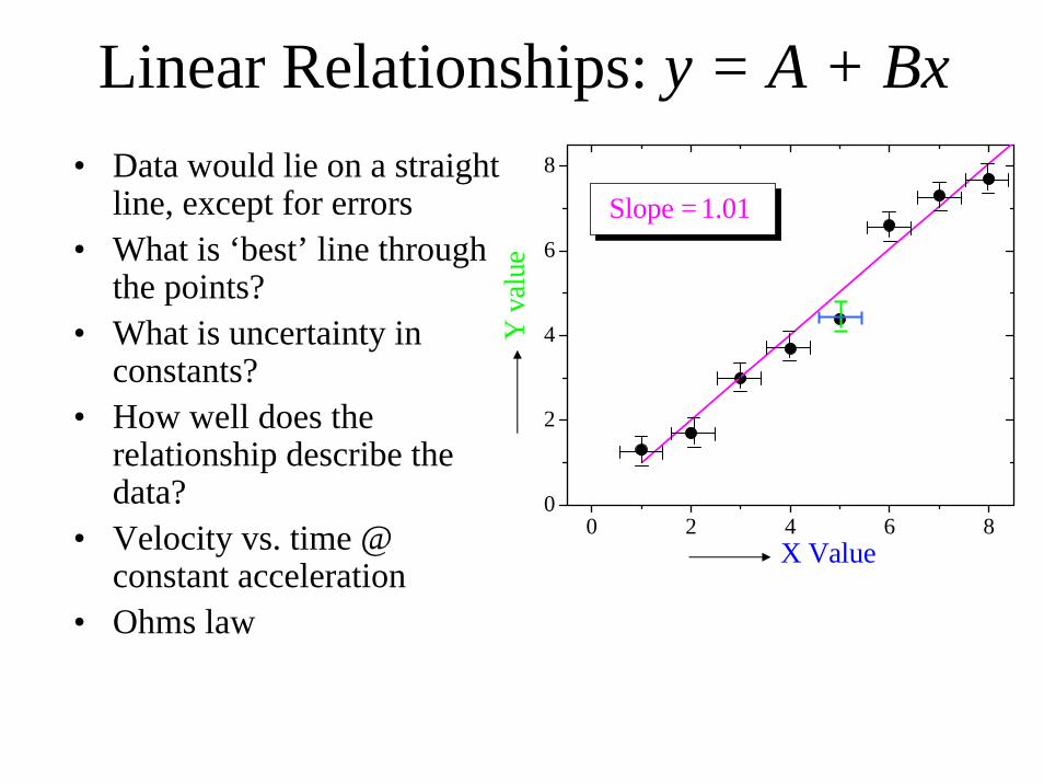
Linear Relationships: y = A + Bx• Data would lie on a straight

line, except for errors• What is ‘best’ line through

the points?• What is uncertainty in

constants?• How well does the

relationship describe the data?

• Velocity vs. time @ constant acceleration

• Ohms law

0 2 4 6 80

2

4

6

8

Slope = 1.01

Y v

alue

X Value

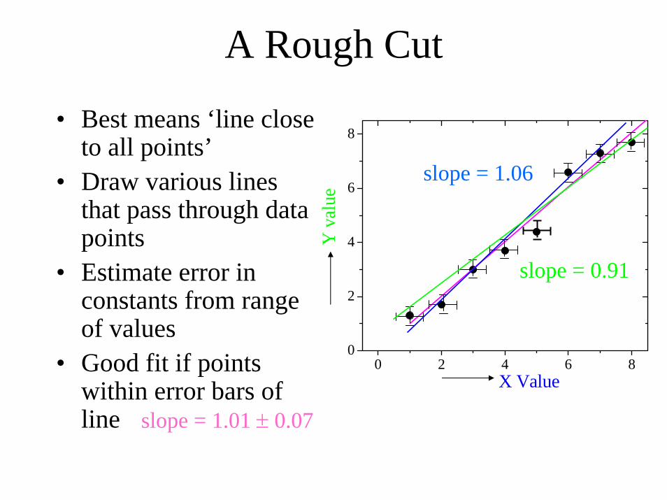
A Rough Cut

• Best means ‘line close to all points’

• Draw various lines that pass through data points

• Estimate error in constants from range of values

• Good fit if points within error bars of line

0 2 4 6 80

2

4

6

8

Y v

alue

X Value

slope = 1.06

slope = 0.91

slope = 1.01 ± 0.07

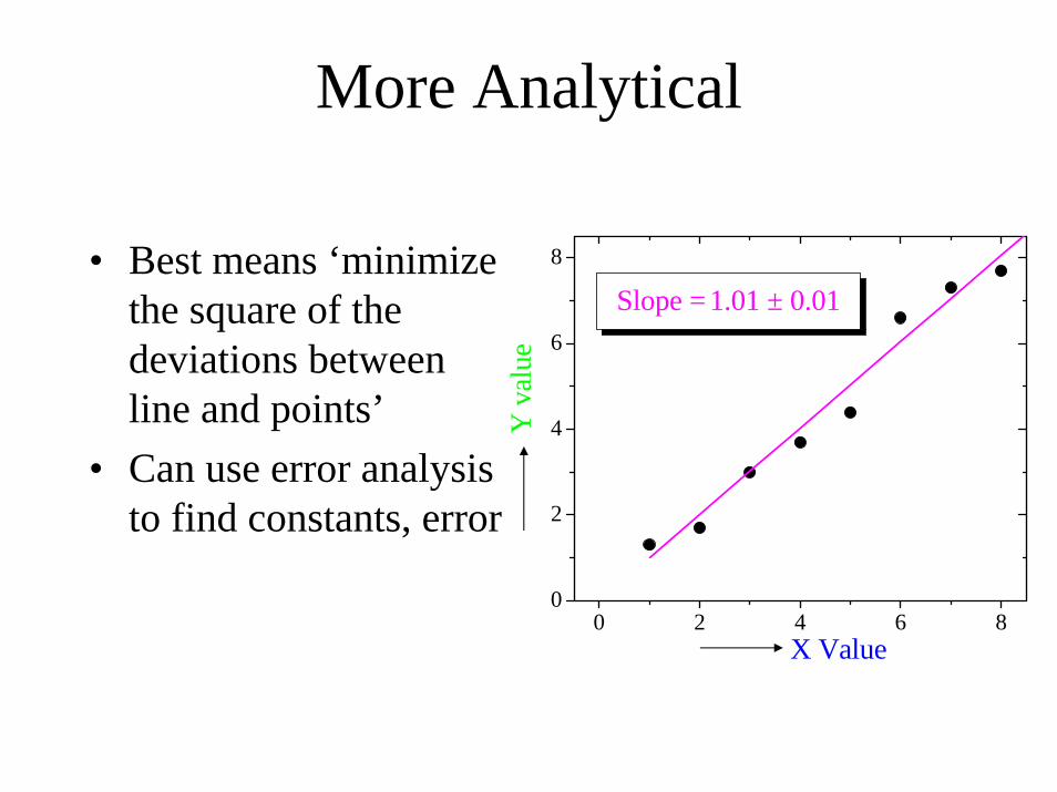
More Analytical

• Best means ‘minimize the square of the deviations between line and points’

• Can use error analysis to find constants, error

0 2 4 6 80

2

4

6

8

Slope = 1.01 ± 0.01

Y v

alue

X Value

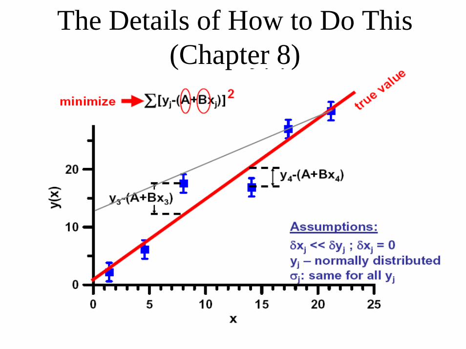
The Details of How to Do This (Chapter 8)

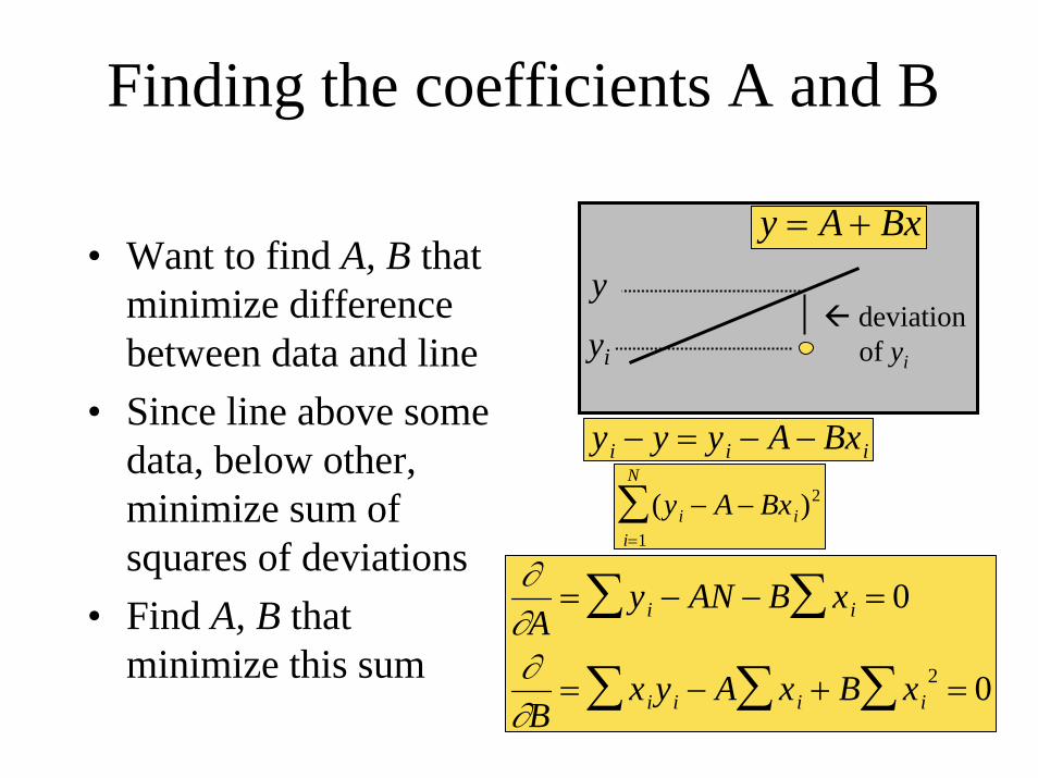
Finding the coefficients A and B

y = A + Bx

yi − y = yi − A − Bxi

(yi − A − Bxi)2

i=1

N

∑∂∂A

= yi∑ − AN − B xi∑ = 0

∂∂B

= xiyi∑ − A xi∑ + B xi2∑ = 0

deviationof yi

y

yi

• Want to find A, B that minimize difference between data and line

• Since line above some data, below other, minimize sum of squares of deviations

• Find A, B that minimize this sum

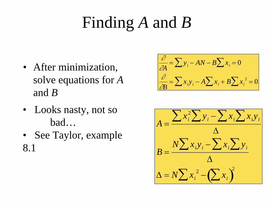
Finding A and B

∂∂A

= yi∑ − AN − B xi∑ = 0

∂∂B

= xiyi∑ − A xi∑ + B xi2∑ = 0

• After minimization, solve equations for A and B

• Looks nasty, not so bad…

• See Taylor, example 8.1

A =xi

2∑ yi∑ − xi xiyi∑∑∆

B =N xiyi∑ − xi∑ yi∑

∆

∆ = N xi2∑ − xi∑( )2

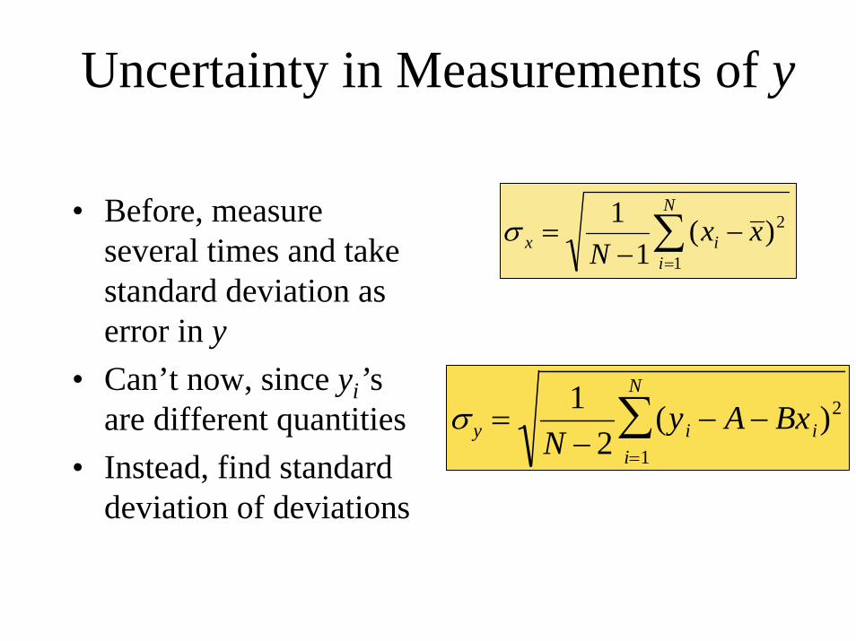
Uncertainty in Measurements of y

∑=

−−

=N

iix xx

N 1

2)(1

1σ• Before, measure several times and take standard deviation as error in y

• Can’t now, since yi’sare different quantities

• Instead, find standard deviation of deviations

σ y =1

N − 2(yi − A − Bxi)

2

i=1

N

∑

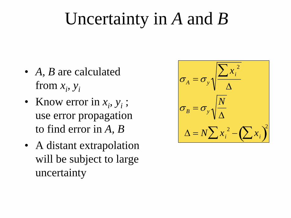
Uncertainty in A and B

σA =σ y

xi2∑

∆

σB =σ yN∆

∆ = N xi2∑ − xi∑( )2

• A, B are calculated from xi, yi

• Know error in xi, yi ; use error propagation to find error in A, B

• A distant extrapolation will be subject to large uncertainty

Uncertainty in x

actualerror in x

equivalent error in y

• So far, assumed negligible uncertainty in x

• If uncertainty in x, not y, just switch them

• If uncertainty in both, convert error in x to error in y, then add errors

∆y = B∆xσ y (equiv) = Bσ x

σ y (equiv) = σ y2 + Bσ x( )2

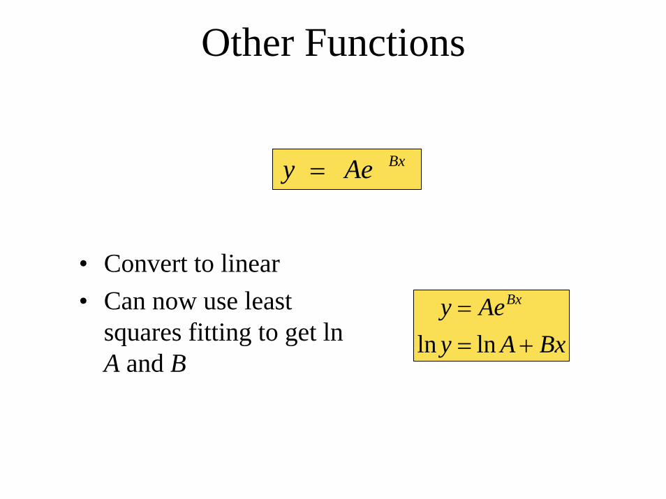
Other Functions

BxAey =

• Convert to linear• Can now use least

squares fitting to get lnA and B

y = AeBx

ln y = ln A + Bx

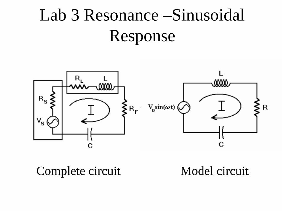
Lab 3 Resonance –Sinusoidal Response

Complete circuit Model circuit

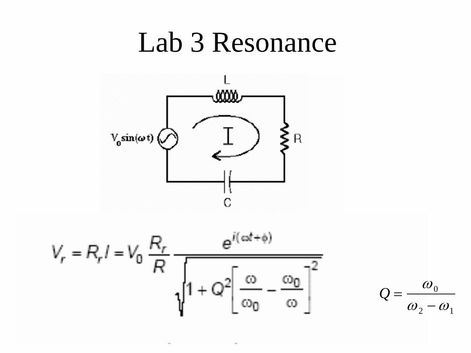
Lab 3 Resonance

Q =ω 0

ω 2 −ω1

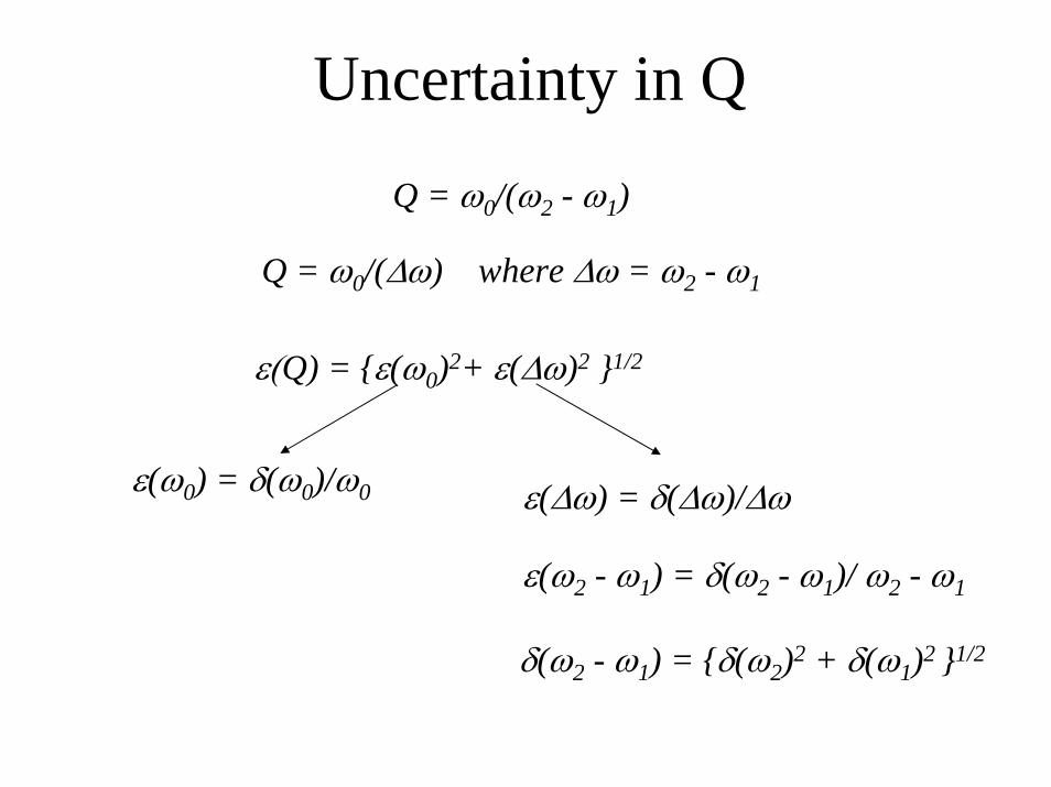
Uncertainty in Q

Q = ω0/(ω2 - ω1)

Q = ω0/(∆ω) where ∆ω = ω2 - ω1

ε(Q) = {ε(ω0)2+ ε(∆ω)2 }1/2

ε(ω0) = δ(ω0)/ω0 ε(∆ω) = δ(∆ω)/∆ω

ε(ω2 - ω1) = δ(ω2 - ω1)/ ω2 - ω1

δ(ω2 - ω1) = {δ(ω2)2 + δ(ω1)2 }1/2

Voltage Response

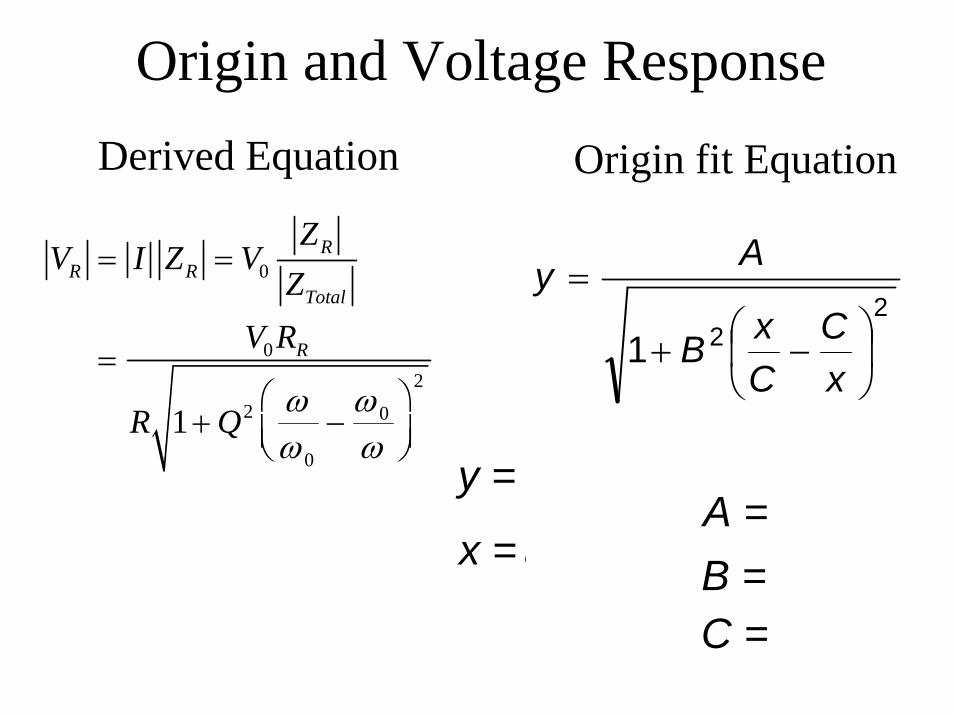
Origin and Voltage ResponseDerived Equation Origin fit Equation

VR = I ZR = V0

ZR

ZTotal

=V0RR

R 1+Q2 ωω 0

−ω 0

ω⎛⎝⎜

⎞⎠⎟

2

221 ⎟

⎠

⎞⎜⎝

⎛ −+

=

xC

CxB

Ay

y = VRA = V0RR/RB = QC =ω0

x =ω

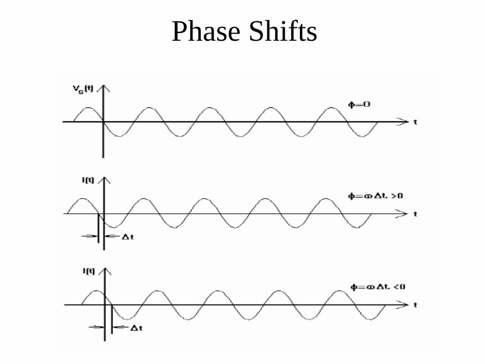
Phase Shifts

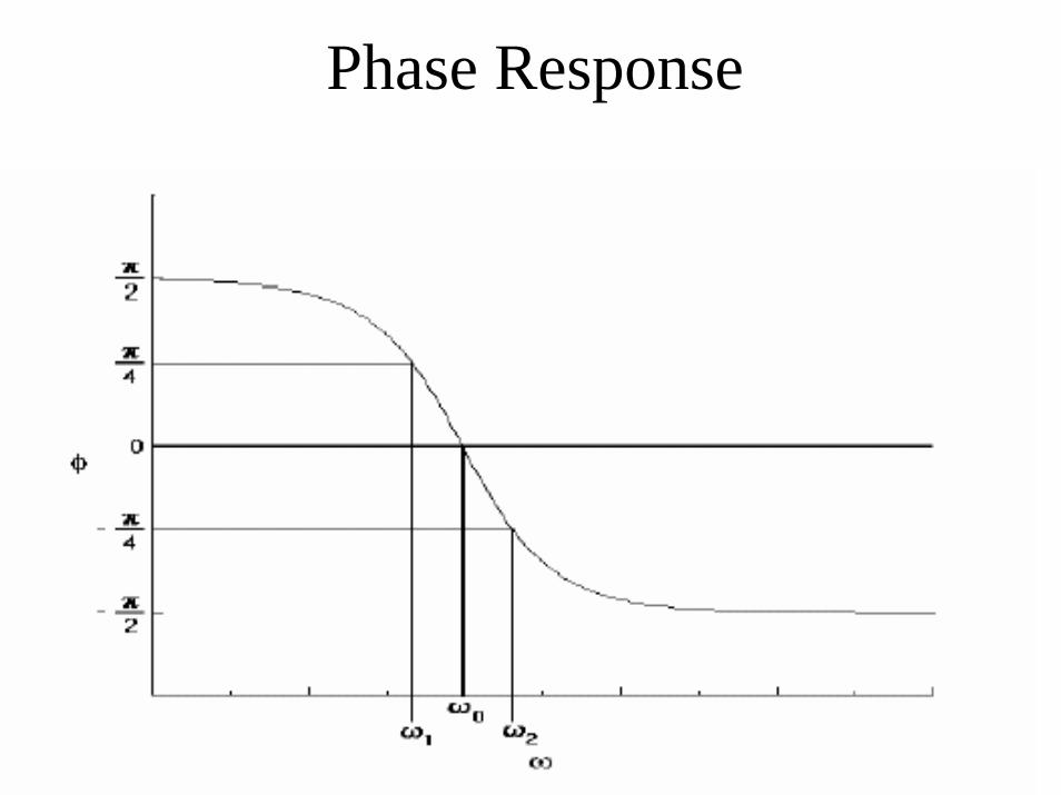
Phase Response

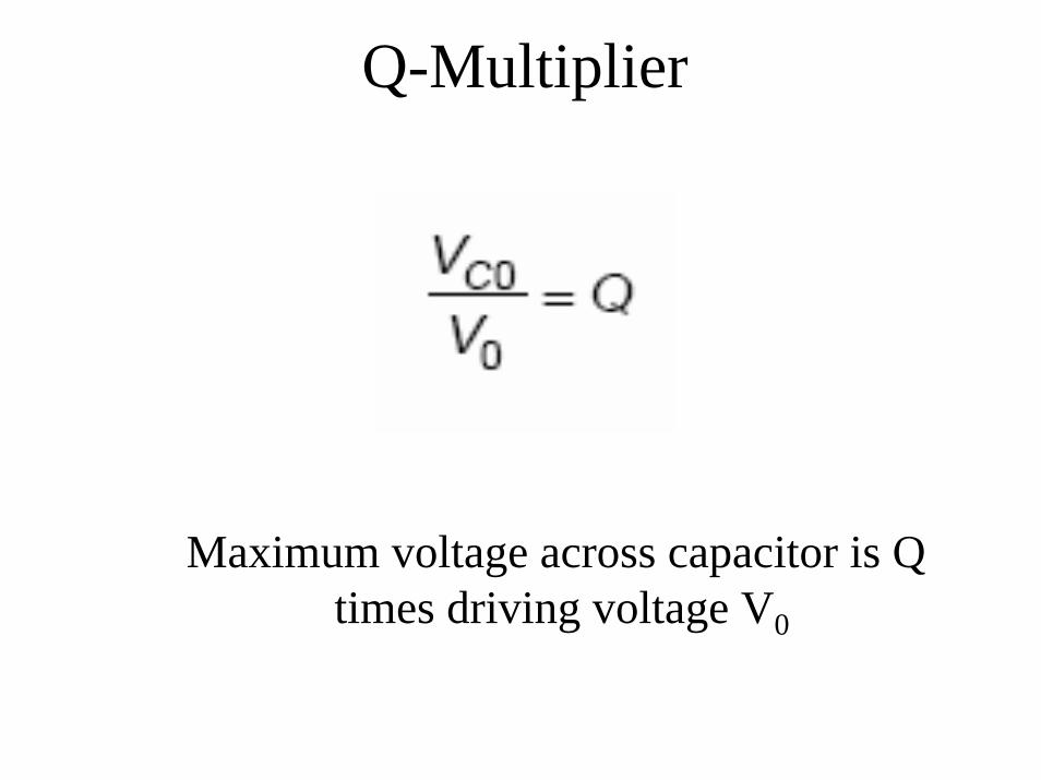
Q-Multiplier

Maximum voltage across capacitor is Q times driving voltage V0

Outline Lab # 3

1). Preliminary calculations of ω0 and Q2). Measure ω0 and Q3). Graph Frequency Response4). Measure Phase Shifts5). Q-Multiplier6). Phase of VC7). Dependence of Q on R

Last set of labs

• Topics include: – Exp. 4: Microwaves: refraction & interference– Exp. 5: Laser: interference, diffraction– Exp. 6: Human eye: lens equation, lens in series

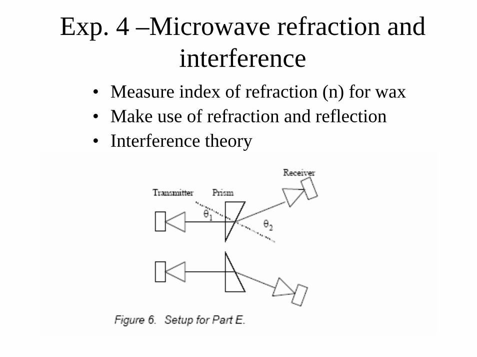
Exp. 4 –Microwave refraction and interference

• Measure index of refraction (n) for wax• Make use of refraction and reflection• Interference theory

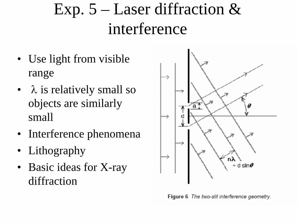
Exp. 5 – Laser diffraction & interference

• Use light from visible range

• λ is relatively small so objects are similarly small

• Interference phenomena• Lithography• Basic ideas for X-ray

diffraction

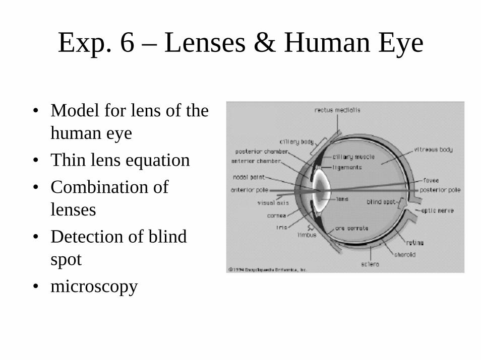
Exp. 6 – Lenses & Human Eye

• Model for lens of the human eye

• Thin lens equation• Combination of

lenses• Detection of blind

spot• microscopy

Remember

• Lab Writeup• CAPE evaluations• Sign-up sheet for last set of labs• Read next week’s lab descriptions, do

prelab• Homework 6 (Taylor 8.1, 8.6, 8.10)