University of ConnecticutOpenCommons@UConn

Doctoral Dissertations University of Connecticut Graduate School

7-31-2014

Essays on the Causes and Consequences of ChildLaborElizabeth KaletskiUniversity of Connecticut - Storrs, elizabeth.kaletski@uconn.edu

Follow this and additional works at: https://opencommons.uconn.edu/dissertations

Recommended CitationKaletski, Elizabeth, "Essays on the Causes and Consequences of Child Labor" (2014). Doctoral Dissertations. 523.https://opencommons.uconn.edu/dissertations/523

Essays on the Causes and Consequences of Child Labor

Elizabeth Ann Kaletski, PhD

University of Connecticut, 2014

The purpose of this research is to examine the causes and consequences of child labor. The first chapter of

this work examines the empirical relationship between working and educational expenditure budget shares

for children ages 5-14 in Mexico. The results indicate that working increases school expenditure share for

working children. In particular, on average, girls engaged in paid work have total annual education

expenditure shares that are 49% higher than girls who do not work. This relationship varies significantly

with characteristics of both the individual and the household, including the child’s gender and type of work

performed, as well as the household’s income, location, and relative female bargaining power. The second

chapter explores the differential impact of migration by male and female household members on household

decision making and child outcomes. Using household and individual level data from four rounds of the

Indonesian Family Life Survey and exploiting an instrumental variables approach, this paper shows that

migration has the ability to causally impact child outcomes and that in some cases these impacts differ

based on the gender of the migrants. Specifically, we find that as the total number of household migrants

increases, both the probability that a child works and his actual work hours decline. On the other hand, the

total number of migrants has no impact on school attendance, but children in households with only female

migrants are less likely to attend school overall. The final chapter examines the impact of state level political

reservation for two minority groups, namely Scheduled Castes and Scheduled Tribes, on child labor in

India. We estimate the effect of political reservation on child labor by exploiting the state variation in the

share of seats reserved for the two groups in state legislative assemblies mandated by the Constitution of

India. Using data from state and household level surveys on fifteen major Indian states, we find that at the

household level, Schedule Tribe reservation decreases the incidence of child labor, while Scheduled Caste

reservation increases the total number of children working.

i

Essays on the Causes and Consequences of Child Labor

Elizabeth Ann Kaletski

B.S., Clemson University, 2008

M.A., University of Connecticut, 2009

A Dissertation

Submitted in Partial Fulfillment of the

Requirements for the Degree of Doctor of Philosophy

at the

University of Connecticut

2014

ii

Copyright by

Elizabeth Ann Kaletski

2014

iii

APPROVAL PAGE

Doctor of Philosophy Dissertation

Essays on the Causes and Consequences of Child Labor

Presented by

Elizabeth Ann Kaletski, B.S., M.A.

Major Advisor_________________________________________________________________________

Susan Randolph

Associate Advisor______________________________________________________________________

Nishith Prakash

Associate Advisor______________________________________________________________________

Delia Furtado

University of Connecticut

2014

iv

Acknowledgements

I could never have completed this work or accomplished my goals without the guidance and

support of many individuals. First, I would like to thank my major advisor, Professor Susan Randolph, for

instilling in me the qualities of being a curious and effective researcher. Her enthusiasm and trust have

been a major driving factor through my graduate career at the University of Connecticut. I would like to

thank my committee members, Professor Nishith Prakash and Professor Delia Furtado, for their

invaluable guidance and unwavering support. The past year has been particularly demanding and yet they

were always willing to provide advice and solutions to the inevitable problems that arise in this sort of

endeavor. A special thanks to my fellow PhD student, Paul Tomolonis for his emotional encouragement

and “life” advice. In addition, numerous faculty aided my development and provided feedback through

the past several years. Thank you to Professor Lanse Minkler, Professor Kathleen Segerson, Professor

Shareen Hertel, and Professor Richard Langlois, in addition to all the faculty at the University of

Connecticut that I’ve had the privilege of knowing over the years. Your support and availability both

inside and outside the classroom has been an essential component to my success. I would also like to

thank the numerous participants of the Department of Economics seminar series at the University of

Connecticut for their vital suggestions and assistance throughout my many years of graduate studies.

A special thank you to my family and friends, without whom I wouldn’t have had the opportunity

or strength to make it through the past several years. Your continuing confidence and encouragement has

made me the person I am today.

1

I. Introduction

The purpose of this research is to examine the causes and consequences of child labor. The decision to

send a child to work occurs at the household level, but is also significantly impacted by factors at the

individual and state levels. Further, the actual working status of the child will affect both individual and

household level outcomes.

In determining the basic causes of child labor, most economists take the position that it is the result of

poverty. Assuming that adults work full time, they hypothesize that children are sent to work only if income

falls short of subsistence consumption (Basu & Tzannatos, 2003).1 Therefore there is still a general belief

that increases in income, or decreases in poverty, is the most important link to a decrease in child labor.

Generally, we can say that child labor is a short run mechanism which families are forced to engage in

during extremely difficult times (Basu & Van, 1998). In addition to the importance of poverty, the child

labor decision is also related to the availability and quality of education, the presence of financial markets

or absence of credit constraints (Jafarey & Lahiri, 2002; Dehejia & Gatti, 2005; Edmonds, 2005), the

availability of community targeted programs (Strulik, 2008), social norms and dynasties (Wahba, 2005;

Behrman, 1997; Haveman & Wolfe, 1995), household size and composition (Grootaert & Kanbur, 1995;

Emerson & Souza, 2003), and the ability of the child (Bacolod & Ranjan, 2008).2

Despite the efforts to recognize and prevent child labor, it is still the reality for millions of children.

According to the ILO, in 2008, 215 million children worked illegally. More than half of these children

worked in hazardous jobs, where their health and safety was at risk. An additional 10 million children are

estimated to be caught up in the worst forms, which include prostitution, slavery, and trafficking (Diallo,

Hagemann, Etienne, Gurbuzer, & Mehran, 2010). In the academic as well as popular literature, most see

child labor as harming vulnerable members of society by exposing them to dangerous and exploitative

work. Child labor might also harm children because work interferes with the child’s ability to attend school

1 This results is derived from a theory developed by Basu and Van (1998) which involves both a luxury and

substitution axiom. Basu and Tzannatos (2003) provide a summary of the model. 2 See (Basu & Tzannatos, 2003) for a more complete review of past literature.

2

and thus lowers human capital, leading to a reduction in lifetime earnings that can perpetuate across

generations (Basu & Tzannatos, 2003).3,4

The research presented here is in line with work on both the causes and consequences of child labor.

The first paper will address one of the most obvious concerns by examining the effects of child work on

individual educational expenditures within the household. This also involves exploring the mechanisms

through which the relationship occurs. In particular, a positive relationship between working and

educational expenditures is consistent with the idea that children have incentives to work. Expanding on

this research, the second paper examines how household migration impacts both decision making in the

household and child labor market outcomes. In particular, it is possible that migration leads to a shift in the

bargaining power of all household members, which in turn potentially impacts the incidence of child labor

in the household. The relationship may be dependent on the gender of both the migrants and the child. The

third paper takes a broader approach by examining how government policies impact the child labor

decisions of the household. More specifically, it estimates how India’s controversial and sweeping

affirmative action policies, which reserve government jobs for minorities, impact the incidence of child

labor at the household level. All of this work is informative for future policy design regarding child labor,

education, migration, and affirmative action.

3 Lower educational levels are also correlated with higher infant mortality and fertility, poor health, and a low life

expectancy (Tauson, 2009). 4 On the aggregate, this is also thought to translate into a system of state level poverty, where human capital

investment remains low, leading to low productivity and technology advancement, which in turn slows growth

(Binder & Scrogin, 1999).

3

Chapter 1: Work versus School? The Effect of Work on Educational

Expenditures for Children in Mexico

I. Introduction

Child labor is an issue of worldwide concern. In the academic as well as popular literature, most

see child labor as harming vulnerable members of society by exposing them to dangerous and exploitative

work. Child labor might also harm children because work interferes with the child’s ability to attend school

and thus lowers human capital, leading to a reduction in lifetime earnings5 that can perpetuate across

generations (Basu & Tzannatos, 2003).6

It is important to keep in mind, however, that not all child employment harms child welfare. Some

jobs, such as apprenticeships, may actually increase human capital formation above what is gained in formal

schooling.7 Moreover, work and school investments may be complements rather than substitutes.8 Blunch

and Verner (2000) point out that in more developed countries children perform household chores or work

in the labor market to finance their own personal consumption. In a developing world context, child work

may allow families to direct a larger share of the household budget towards education expenditure, thus

actually improving educational outcomes.

This paper tests whether child labor adversely impacts child welfare, with specific focus on the

relationship between working and education. In order to explore this, I look at the empirical relationship

between working and education expenditure budget shares for children ages 5-14 in Mexico. This will be

accomplished using the Mexican Family Life Survey (MxFLS), a panel dataset available in 2002 and 2005.

5 Lower educational levels are also correlated with higher infant mortality and fertility, poor health, and a low life

expectancy (Tauson, 2009). 6 On the aggregate, this is also thought to translate into a system of state level poverty, where human capital

investment remains low, leading to low productivity and technology advancement, which in turn slows growth

(Binder & Scrogin, 1999). 7 The International Labour Organization (ILO) recognizes that “children’s or adolescents’ participation in work that

does not affect their health and personal development or interfere with their schooling, is generally regarded as

being something positive… [Some jobs] contribute to the children’s development and to the welfare of their

families; they provide them with skills and experience and help to prepare them to be productive members of society

during their adult life” (International Labour Organization, 2013). 8 In the Mexican context, enrollment rates are known to be high for both female and male children. In the data used

in this analysis, enrollment rates are near 100% for both male and female children regardless of their work status.

This is likely due to the fact that education is compulsory and provided free by the government through grade 9.

4

The benefit of this dataset lies in its detailed information on child work as well as education expenditures

at both the household and individual level.9

Although there are many studies which seek to explore the allocation of resources within the

household,10 few studies have done so in the context of child labor. One exception is Moehling (2006), who

uses household level Engel curves and U.S. historical data to explore the relationship between child income

and household budget shares. She finds that earnings from children alter household resource allocation by

shifting consumption from private goods such as father’s clothing, to publicly consumed goods, particularly

food expenditures. In addition, there are few studies which explore the empirical relationship between

children working and expenditures using individual level data.11 Again, one exception is Moehling (2005)

where the same data are used to explore the impact of working on an individual child’s private clothing

expenditure. She finds that working children have higher clothing expenditures than non-working children,

and that expenditures are increasing in the amount of child income earned.

However, to my knowledge, this is the first paper to examine the relationship between working

children and education expenditure shares using individual level data.12 The benefit of acquiring data on an

individual child’s expenditure, as opposed to goods that are simply assignable to adult or child household

members,13 is that we can see the direct impact of that child’s labor market outcome on his household

resource allocation. As will be discussed further below, theory provides multiple channels through which

child work can be associated with education expenditure shares. Understanding this relationship, along with

9 The survey also includes data on health expenditures for individual children, but the results are omitted from this

paper due to the fact that observations are limited, no clear pattern emerges in the analysis, and federal law actually

requires regular health check-ups for working children. 10 For example, see Deaton (1987, 1989), Hoddinott & Haddad (1995), Vermeulen (2005), Duflo & Udry (2004),

Lancaster et al. (2008), Zimmerman (2011) to name only a few. Many of these studies are also constrained by the

use of adult assignable goods. 11 This is not to say that others haven’t explored household allocations with individual level data. For example, see

Deolalikar (1997) and Irving & Kingdon (2008). However, none of these studies include an analysis of how child

work impacts these allocations. 12 The idea that child work negatively impacts educational outcomes is common in the child labor literature, but

looking at the relationship between work and expenditures provides new insights by exploring the actual education

allocation for a given child. It should also be noted that this is the only sufficient measure of private consumption

available in the survey. 13 Adult assignable goods are those which are consumed by adult household members as opposed to child household

members. Common examples include tobacco, alcohol, and adult clothing (Deaton, 1997).

5

the mechanisms through which it occurs is essential for constructing effective policy in regards to both

child labor and education.

My results indicate that engaging in paid work has the ability to increase school expenditure shares

for working children. In particular, on average, girls in paid work have education expenditure shares that

are 48.73% higher than girls who are not working. This translates into an average education budget share

that increases from 1849.91 to 2751.34 Mexican pesos annually.14 However, this relationship varies

significantly by individual characteristics including gender and the type of work performed, as well as

household characteristics, such as income, location and female bargaining power. The results indicate that

working does not appear to translate into a decrease in welfare15 and the additional expenditure is directed

towards goods that improve the quality of education. These relationships are explored further in the results

section of the paper.

The rest of the paper will be structured as follows; Section II discusses relevant background

literature and the conceptual approach used in this paper. Section III presents the empirical framework,

while Section IV describes the data. Section V presents the baseline results, along with evidence regarding

heterogeneity and robustness. Section VI is left for discussion and conclusions.

II. Background and Conceptual Approach

For international policy purposes, child labor is defined as the number of economically active

children under the age of 15 years.16 As with most other countries across the world, regulation of child labor

in Mexico comes in the form of laws restricting its practice. Although Mexico has not yet ratified ILO

Convention 138 on the minimum age of employment, at the national level the Mexican Constitution

14 This is an increase of 901.44 pesos, which translates into about 83 dollars annually. The results section will

provide additional details on the type of goods this money is spent on. 15 It should be noted here that in this analysis, welfare is measured by private consumption expenditure. I also

explore the impact of work on additional educational outcomes including, but not limited to attendance and grade

repetition. These results are presented in Table 10. This definition does not include every aspect of welfare and has

notably ignored any other impacts on the child’s development, health and nutrition. 16 This is set at 14 years in specific developing countries. The exact definition also depends on the type of work,

hours performed, and the impact on the health and education of the child.

6

establishes 14 as the basic minimum age for work. Part of the Constitution, the Federal Labor Law (LFT)

discusses the specifics regarding working children, including limiting work time to six hours a day, along

with requiring permission from a legal guardian and regular medical checkups. It also prevents any work

that is dangerous or unhealthy, underground or underwater. The federal government is responsible for

enforcement in some cases,17 but in most cases falls under the jurisdiction of the state (Bureau of

International Labor Affairs). Despite these regulations and a World Bank classification as an upper middle

income country, in 2004, it was estimated that 9% of children in Mexico between the ages of 7 and 14 were

engaged in work (The World Bank Group, 2013b).18

Based on previous literature, there are many potential relationships between working and education

expenditure shares within the household. First, it is possible that there is no statistically significant

relationship. This is likely to be true under the traditional unitary model in which the household maximizes

one welfare function subject to a single joint budget constraint. Practically, this implies that the household

behaves as though they are a single decision making unit (Vermeulen, 2002) and the source of income is

irrelevant. Applications of the unitary household model to the child labor literature lead to the conclusion

that children’s income from working would be shared by everyone in the household through a relaxed

budget constraint.19, 20 An insignificant relationship is also consistent with the idea that households simply

expect boys to work, that boys are altruistic towards the household, or that boys’ income is used for other

purposes. In any of these cases, we would not expect to find a significant relationship between working and

education expenditure shares.

17 For example the federal government is responsible in the case of textiles, chemicals, automobiles and metals. 18 This has been recalculated by the World Bank and only includes their definition of “economically active”

children. It does not include unpaid household services. 19 The unitary household assumption in the child labor literature is supported by the fact that many children actually

work within the household and any schooling is typically financially supported by parents (Edmonds, 2008). 20 It should be noted that although the unitary approach is common in modeling the child labor decisions of the

household, the unitary model itself has been criticized heavily on both theoretical and empirical grounds in the last

twenty years. Some criticisms include the importance of methodological individualism and resource allocation

within the household, and how this translates into education, food, and human capital investment for specific

individuals (Vermeulen, 2002).

7

On the other hand, the literature has also indicated a potential negative relationship between child

work and education expenditure shares. One possibility comes directly out of the idea that every individual

is faced with time constraints, and thus if a child goes to work, less time is left for schooling and leisure.

Edmonds (2008) documents that on average, school attendance rates are lowest and hours worked are

highest among children in market work outside the household.21 However, in the Mexican case, many

children have the ability to simultaneously attend school and engage in work. I explore this relationship

further in the results section of the paper using detailed information on the paid work hours per week for

each child. An additional mechanism behind a negative correlation could be that child income is treated as

a separate account in the household expenditure decision. As Moehling (2006) points out, according to

Basu and Van (1998) the “luxury axiom” indicates that parents only send children to work when

consumption falls below a subsistence level. Thus parents prefer not to send children to work, and only do

so when it is necessary for household survival. If this is correct, we would expect child income to go towards

paying off debts or to essential goods (Moehling, 2006). The empirical results then depend on how the

household classifies the good in question.

However, this last point also provides a channel through which child work can have a positive

impact on education expenditures. More specifically, in the above context, if education expenditures are

considered a necessary good within the household, then working should lead to higher education

expenditure shares. In line with this idea, a positive relationship between child work and education

expenditure shares could exist if working actually helps the child attend school. In this situation,

contributing to household income through work could induce an increase in the education budget share

without interfering with the child’s ability to attend school. These ideas provide evidence that total

household income plays an essential role in the relationship between work and education. More specifically,

we would expect the relationship to be stronger for households below the poverty line, where the budget

constraint is especially binding, than for those above it. This idea is explored further in the results section.

21 See Edmonds (2008) for a review on the relationship between work and schooling attendance, attainment and

achievement.

8

Additionally, an increase in education expenditure shares for working children would be consistent

with a unitary or collective bargaining model of household decision making. More precisely, the positive

relationship could be the result of parents rewarding children for working22 or the child gaining power

within the household through work.23, 24 This leads to the idea that children may actually have incentives to

work. Moehling (2005) provides the best evidence of this concept by historically looking at the role of

children in the family decision making process. Using data from the Bureau of Labor Statistics Cost of

Living Survey 1917-1919, she shows that despite the fact that at that time working children turned almost

all of their earnings over to their parents, they still had higher clothing expenditures than non-working

children. Further, their clothing expenditures were increasing in the amount of income they earned.

Thus as in Moehling (2005), the child may have a financial incentive to choose to work or to

cooperate with their parent’s desire to send them to the labor market. Regardless of whether the child makes

an independent decision or whether he simply has the ability to express his preferences to his parents,

compensation within the household may be one way in which households induce children to work. If we

believe this to be true we would expect the relationship to be stronger for older children, who better

22 The first model which incorporates child behavior is attributed to Becker (1974). This model involves a self-

interested child who is induced to act in an unselfish and efficient manner through transfers from his altruistic

parent. In the child labor literature, this would be similar to the idea that parents compensate children for their work

by increasing the amount of household expenditures they earn. 23 Due to criticisms of the unitary model, numerous alternatives emerged which specifically sought to focus on the

individual and differing preferences of household members (Manser and Brown, 1980; McElroy and Horney, 1981;

Lundberg and Pollack, 1993 to name a few). One such set of models are known as collective bargaining models in

which each person in the household has different preferences and bargaining between those individuals is what

determines the allocation of resources (Vermeulen, 2002). In addition, many have conducted empirical tests of these

collective household models and have shown that the source of income has a significant effect on household

resource allocation (Fortin & Lacroix, 1997). For example, Browning et al. (1994) use Canadian data to show that

allocations of expenditure depend significantly on relative incomes, ages and lifetime wealth of respective

household members (Also see Hoddinott and Haddad (1995), Udry (1996), Maitra & Ray (2002), Duflo & Udry

(2004)). In fact the idea of pooling income within a household, which is the main property of unitary models

(Chiuri, 2000), has been strongly rejected (Moehling, 2005). Instead much of this literature has indicated that the

power of a particular individual determines household outcomes (Moehling, 2006). 24 The concept of child agency in household decision making is controversial, but increasingly interesting. There is a

small set of literature which show that children are rational actors (Harbaugh et al. 2001), they understand the

bargaining process (Harbaugh et al., 2003), and they independently influence household consumption and activities

(Dauphin et al., 2011; Lundberg et al., 2009). Iverson (2002) also finds anecdotal evidence that boys ages 13 and 14,

exhibit autonomy and independence in their decisions to enter the labor force or avoid education. Further, through a

field experiment, Berry (2013) finds differential impacts of giving incentives to children over adults in educational

outcomes.

9

understand their labor market opportunities and can articulate their preferences. Further, we expect different

levels of compensation depending on the type of work the child is engaged in. If paid work is more difficult

or time consuming than working within the household, a child should be compensated at a higher rate. Our

data allows us to explore both of these factors in the results section below.

The numerous potential relationships between work and education expenditure shares lead to the

conclusion that this relationship is likely to vary with aspects of the child and the household. The most

important characteristic to impact the relationship is the child’s gender. This stems out of the idea that girls

and boys typically engage in different types of work, which require diverse time commitments and are also

treated differentially within the household. Thus the baseline regression tries to account for these

differences by focusing on the impact of paid work for girls and boys age 5-14 separately. Following this

baseline, I then explore additional heterogeneity and robustness of the results.

III. Empirical Framework

The approach of this analysis involves empirically examining how individual education

expenditure shares vary with a child’s labor market outcomes. One major issue with this type of exercise is

that we would have to assume the demand for goods and labor supply decisions are independent within the

household. However, it is more likely that these decisions are made simultaneously. More specifically,

labor supply is endogenous to the household expenditure decision in that the presence of working children

is likely correlated with other household characteristics which affect household expenditure allocations.

Some of the characteristics are observable, such as household size, the age and sex composition of

household members, and expenditure per capita. For example, households with fewer children, but the same

income will have more to spend per capita on every member of the household and are less likely to send

children to work.25 Controlling for household income is also particularly important because households

25 Grootaert & Kanbur (1995) use Becker’s (1960) quantity-quality tradeoff regarding fertility decisions to suggest

that larger households reduce educational participation of children as well as the investment in education that

parents make.

10

with higher income will have more to spend on child related goods and will find child work less necessary.26

Failing to control for these observable omitted variables will bias our estimates, though the direction of the

bias is not entirely clear.27

In addition to these characteristics, which are common in Engel curve specifications of the gender

discrimination literature,28 there are likely other important socioeconomic factors which influence child

expenditures. In particular, characteristics of the household head including gender, education and

employment status, as well as the location and ownership status of the house will affect how resources are

allocated (Kingdon, 2003).29 For example, numerous papers assert that women with higher levels of

education are more likely to invest in children’s goods and other factors that will improve overall household

welfare.30 Further, as we have individual level data, characteristics of the individual child, such as his age

and whether he receives a scholarship, will determine both expenditure and labor market decisions.31, 32

Fortunately, many of these aspects can be and are controlled for in this analysis. Accounting for these

household and individual level characteristics reduces any omitted variable bias and helps get a clearer

picture of the relationship between work and education expenditure shares.

26 Here expenditure per capita is a proxy of household income. As Lancaster et al. (2008) note, household

expenditure is easier to measure, less prone to measurement error, and is less subject to transitory fluctuations.

Further, in the data used here, expenditures receive a much higher response rate than questions regarding household

income. However, it should be noted that this may be correlated with other unobserved determinants of budget

shares and thus these regressions are run without including expenditure per capita as well. 27 For instance, household size is likely to be positively correlated with child work, but negatively correlated with

expenditure shares. On the other hand, income is negatively correlated with child work and positively correlated

with expenditure shares. 28 For examples in the gender discrimination literature see Case and Deaton (2003), Gong et al (2000), Lancaster et

al (2008), Irving & Kingdon (2008) 29 Similar characteristics are controlled for in multiple studies including Deolalikar (1997) 30 As a specific example, Bobonis (2009) shows that women’s income compared to overall household income is

more often used for these reasons. Although the main specification doesn’t include women’s income directly, I

control for the gender of the household head. The data does provide a measure of female income share, which can be

used to proxy for bargaining power. However, due to low response rates, including female income share as a control

in our baseline regression reduces sample size by more than half. It should be noted that although it is an important

factor in the analysis it does not qualitatively change the results. Thus this measure is reserved as a robustness check

in the results section. 31 Similar characteristics are controlled for in many other studies including (Aslam and Kingdon, 2008). 32 It should be noted here that the majority of the gender discrimination literature looks at the impact of girls versus

boys by using adult or child assignable goods at the household level. The availability of individual level data allows

this study to look directly at the impact on the individual child. This provides a much clearer picture of the

relationship between expenditure shares and working.

11

Thus, I estimate Engel curves linking expenditures on individual goods with total expenditures and

demographic characteristics of the household. The functional form used here is drawn from Working-Leser

(1943, 1963). The benefits of this specification are in its simplicity as well as the fact that it conforms to

the data in a wide range of circumstances (Deaton, 1997). Following Moehling (2006), I can then augment

the original Working-Leser equation to include the concept of child labor in the following way:

𝑤𝑗𝑖𝑡 = 𝛼 + 𝛽 ln (𝑥𝑖𝑡

𝑛𝑖𝑡) + 𝛿 ln(𝑛𝑖𝑡) + ∑ 𝛾𝑘

𝐾−1𝑘=1 (

𝑛𝑘𝑖𝑡

𝑛𝑖𝑡) + 𝒁𝒊𝒕𝜏 + 𝑪𝒋𝒊𝒕𝜌 + 𝜇𝐶ℎ𝑖𝑙𝑑𝑊𝑜𝑟𝑘𝑗𝑖𝑡 + 휀𝑗𝑖𝑡 (1)

where 𝑤𝑗𝑖𝑡 is the education budget share of child 𝑗 in household 𝑖 at time 𝑡. 33 𝑥𝑖𝑡 is the total expenditure

of household 𝑖 at time 𝑡, 𝑛𝑖𝑡 is household size, and thus ln (𝑥𝑖𝑡

𝑛𝑖𝑡) is the natural log of expenditure per capita

in the household.34 ln(𝑛𝑖𝑡) is included to allow for the household size to independently impact expenditure

shares on certain goods. As in the gender discrimination literature, 𝑛𝑘𝑖𝑡

𝑛𝑖𝑡 is the fraction of household members

in age-sex class 𝑘, where 𝐾 is the total number of age-sex classes. This will include the fraction of males

age 0-4, females age 0-4, males age 5-14, females age 5-14, males age 15-54, females age 15-54 and males

age 55 and over. Since the fraction of household members adds up to unity, one must be omitted in the

regression; in this case the category of females over the age of 55. 𝒁𝒊𝒕 is a vector of other household

characteristics including a dummy equal to one if the household is in an urban area,35 a year dummy, the

household head’s sex, education, and employment status, and a dummy equal to one if the household owns

its residence. 𝑪𝒋𝒊𝒕 is a vector of individual characteristics including the child’s age and a dummy variable

equal to one if he receives a scholarship through Oportunidades or any other source, for the specific purpose

33 In this case, we have two time periods 2002 and 2005. 34 This functional form assumes that all households treat education as the same type of good. For instance a negative

coefficient on the log of per capita expenditures implies that education expenditures are a necessary good for these

households. However, it is likely the case that for households with extremely low expenditures, education is

considered a luxury good. In order to explore this I relax the initial assumption by including a quadratic term as a

robustness check in the results section. 35 This is particularly important because in Mexico children in rural areas are much more likely to work than

children in urban areas.

12

of increasing education investment. The main independent variable of interest is 𝐶ℎ𝑖𝑙𝑑𝑊𝑜𝑟𝑘𝑗𝑖𝑡, which is

an indicator equal to one if child 𝑗 in household 𝑖 is engaged in paid work at time 𝑡. 36 In the initial analysis

equation (1) is run as a repeated cross-section using OLS and standard errors are clustered at the household

level. In order to better assess the impacts of including these controls, the regression is first run using only

the child’s age and a year dummy, then adding the Engel curve controls, and finally using the full set of

controls as shown in equation (1). By construction, the sample is restricted to individuals between the age

of 5 and 14.

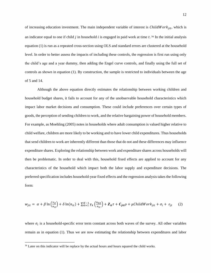
Although the above equation directly estimates the relationship between working children and

household budget shares, it fails to account for any of the unobservable household characteristics which

impact labor market decisions and consumption. These could include preferences over certain types of

goods, the perception of sending children to work, and the relative bargaining power of household members.

For example, as Moehling (2005) notes in households where adult consumption is valued higher relative to

child welfare, children are more likely to be working and to have lower child expenditures. Thus households

that send children to work are inherently different than those that do not and these differences may influence

expenditure shares. Exploring the relationship between work and expenditure shares across households will

then be problematic. In order to deal with this, household fixed effects are applied to account for any

characteristics of the household which impact both the labor supply and expenditure decisions. The

preferred specification includes household-year fixed effects and the regression analysis takes the following

form:

𝑤𝑗𝑖𝑡 = 𝛼 + 𝛽 ln (𝑥𝑖𝑡

𝑛𝑖𝑡) + 𝛿 ln(𝑛𝑖𝑡) + ∑ 𝛾𝑘

𝐾−1𝑘=1 (

𝑛𝑘𝑖𝑡

𝑛𝑖𝑡) + 𝒁𝒊𝒕𝜏 + 𝑪𝒋𝒊𝒕𝜌 + 𝜇𝐶ℎ𝑖𝑙𝑑𝑊𝑜𝑟𝑘𝑗𝑖𝑡 + 𝜎𝑖 + 휀𝑗𝑡 (2)

where 𝜎𝑖 is a household-specific error term constant across both waves of the survey. All other variables

remain as in equation (1). Thus we are now estimating the relationship between expenditures and labor

36 Later on this indicator will be replace by the actual hours and hours squared the child works.

13

market outcomes of children within a given household in a given time period. The variation that remains is

across children within the same household and will be due to their individual characteristics. The benefit of

this approach is that these individuals have been exposed to the same household demographics, relative

prices, and as well as unobservable characteristics.37

One may still be concerned about characteristics which cause households to have different views

and preferences across children. This could potentially occur if the household’s view of child labor differs

by the gender and age of the child. For example, there is some evidence that Mexican parents have a

preference for sons which impacts family structure and decisions (Ruiz & Vazquez, 2013). Further, in the

case of child labor this son preference is likely to result in girls being more likely to work (Kumar, 2013)

and less likely to receive additional education expenditures. In order to account for any differences across

gender and age, equation (2) is run separately for male and female children and linear and quadratic age

variables are directly controlled for.38

One last concern relates to the idea that households may simply prefer one child over another

because they have exhibited a higher ability. This is not a significant problem in this analysis because even

if this were to bias the estimates, it would only bias them downwards. More specifically, as mentioned, I

find a positive significant relationship between educational expenditure shares and working for female

children. If households chose to invest more in an individual girl because they displayed higher ability, this

would likely result in that girl working less and having higher education expenditure shares. Since this bias

works in the opposite direction as the relationship found, it would simply imply that the estimates found

here are an underestimate of the actual effect.

Although I believe equation (2) addresses the main sources of bias, there could be additional

concerns about omitted variables and reverse causality. It is not realistic to completely rule out the

possibility that I have left out a relevant variable, but in order to impact the results presented here it would

37 A similar approach is used in Moehling’s (2005) paper on youth employment and household decision making in

the early twentieth century U.S. 38 Additionally, to allow for flexibility in the role that age plays the robustness checks include a specification where

the child’s age and age squared are replaced by dummy variables for each age from 5 to 14.

14

need to be one that has a strong relationship with child labor or expenditure shares even after controlling

for all the above mentioned factors. Further, reverse causality would imply that an increase in schooling

fees or tuition causes a child to enter the labor market. This is unlikely to be a major issue for several

reasons. For one, as previously discussed, education is provided at no cost by the government and most

children in Mexico are in school regardless of their work status. Further, as the results will show, the

relationship is driven by spending on “extras” which improve the quality of education, but are not required

for attendance. The results presented below will compare the estimates from equation (1) using OLS and

equation (2) using household-year fixed effects.39

IV. Data

The data used in this paper come from the Mexican Family Life Survey (MxFLS). This survey

includes nationally representative longitudinal data with a large base of information on socioeconomic

factors, demographics and health of the Mexican population. The baseline survey was done by the National

Institute of Geography Statistics and Information (INEGI) in 2002 (MxFLS-1). The second wave (MxFLS-

2) contacted 90 percent of the original households in 2005-2006. It includes 8,440 households with

approximately 35,000 individual interviews in 150 different communities throughout Mexico. The

household level survey includes information on expenditures and consumption, education and school

attendance variables, employment characteristics of all household members over the age of 5, time

39 It should be noted that an instrumental variables approach was explored as an additional empirical framework.

This involves identifying a set of instrumental variables that will only influence household expenditures through

their effect on a child’s labor market decision. Thus the instrument considered for children in paid work was whether

or not the household owns a non-agricultural business at the time of the survey. The idea is that if a household owns

a small business, particularly outside of household farming activities, it is more likely that children from that

household contribute to the business thus engaging in paid work. This is reflected in the fact that owning a non-

agricultural business is positively and statistically significantly correlated with both male and female paid work.

Although this instrument appears relevant, it must also be valid, or in other words, uncorrelated with the

unexplained variation in expenditures. In the case of paid work, business expenses are calculated as a separate

category of household expenditures in the survey, thus owning a business should not impact the budget share of

female or male children directly. However, due to the fact that threats to the exclusion restriction may exist (i.e. it is

possible that households that own businesses are better off and therefore have more income to spend on children’s

education in general), the IV approach was left out of the formal analysis.

15

allocation and health status. In addition the survey includes information on important community indicators

and infrastructure (Rubalcava & Teruel, 2008).

Table 1 provides summary statistics at the household level for both rounds of data combined.40

Column 1 shows the statistics for all households with data on children in paid work, while columns 2 and

3 show the differences across households that have working children and those that do not have working

children.41 In this sample, 12.7% of households have a child engaged in paid work. Comparison across

columns indicates that households with working children are larger and more likely to have a household

head that is female and employed than households with non-working children. Further, they are more likely

to be located in a rural area and have a household head with lower educational attainment. They are also

more likely to fall below the median household poverty line and have expenditure per capita that is well

below households with non-working children, which may reflect their overall lower economic status and

hence their need to send children to work.

Table 2 shows summary statistics for individual children broken down by gender. Although the

majority of kids appear to work within the household, 3.7% of girls and 6.8% of boys are engaged in paid

work. In this case household work encompasses tasks such as collecting water or firewood, taking care of

younger siblings and the elderly, doing domestic housework such as sweeping, washing dishes, dusting,

and any agricultural activity including weeding, sowing, and taking care of animals or the family business.

Paid work requires an activity that specifically helps with household expenses by being paid either in cash

or kind. As expected, more boys are engaged in paid employment than girls, but more girls participate in

household work than boys. It should also be pointed out that the hours of work are extremely long for both

girls and boys engaged in paid work, especially relative to household work.

The main dependent variable used in this analysis is the individual child’s education expenditure

share. Education expenditure includes school fees for enrollment, registration, courses, exams and

40 Expenditure data was adjusted for inflation using the Mexican CPI and are in 2005 Mexican pesos. The CPI data

came from OECD Stats and are available at: http://stats.oecd.org/ 41 For the purposes of summary statistics, households with working children are those households that have a child

engaged in paid work in either 2002 or 2005.

16

maintenance, along with spending on school materials such as books, supplies, uniforms and sports, and

any additional expenditure on school celebrations and festivities. Initially, total education expenditure is

used in the baseline regressions, but the impact of working on school fees versus other additional education

expenditure is explored as well. Shares are calculated by dividing annual expenditures on education by total

annual household expenditures. It should be emphasized that expenditure shares are used here as opposed

to levels. The emphasis is on how working impacts household resource allocation among its members.

Table 2 shows that although expenditure shares on education appear similar for boys and girls across all

households, they are much higher for girls engaged in paid work than for boys. The difference in working

and expenditure shares across genders provides additional support for splitting the baseline regression and

analyzing the impacts on girls and boys separately.

V. Working Children and Child Expenditure Shares

a. Baseline Results

Tables 3 and 4 show the results of the baseline regression for girls and boys respectively. The OLS

results from equation (1) are displayed in columns 1 through 3, beginning with a specification that only

controls for the child’s age and the year of the survey, followed by the inclusion of the Engel curves

controls, and then the full specification of equation (1). Column 4 shows the results from the household-

year fixed effects model of equation (2).

The results from these regressions indicate that household demographics are rarely statistically

significant. They do confirm that as the log of household size increases, individual child’s education

expenditure shares fall. Further, the coefficients on the log of expenditure per capita indicate the type of

good as either a necessity or luxury. When this coefficient is greater than zero, the share of the budget

increases with total outlay, so that total expenditure elasticity is greater than one (Deaton, 1997).42 Here the

42 An additional benefit of the Working-Leser specification is that expenditure elasticity can be calculated as:

𝜖 = 1 + (𝛽

𝑤). Thus a negative coefficient on the log of expenditure per capita implies that the good is a necessity.

17

consistently negative and statistically significant coefficient on log of expenditure per capita indicates that

households consider education expenditures as a necessity for both girls and boys.43 Further, these results

indicate that there are non-linear impacts of the child’s age, a relationship that is explored further below.44,45

Beginning with the coefficients of interest for girls in Table 3, engaging in paid work is positively

and significantly correlated with education expenditure shares. The coefficient is stable in magnitude across

all four specifications regardless of the controls included. In the preferred specification of column 4, a

coefficient of .933 represents a 0.93 percentage point increase in education expenditure shares for girls in

paid work. Based on the average girl’s budget share of 1.92% shown in Table 2, this implies a 48.7%

increase in education expenditures for girls engaged in paid work over those who do not work. On average,

this translates into an increase of 901.44 pesos annually from a baseline of 1849.91 pesos.46 The

heterogeneity and potential mechanisms behind this relationship are explored further below.

The relationship for boys in Table 4 is less clear. The coefficients on the primary variables of

interest are consistently negative, but only statistically significant in columns 1 and 2. The magnitude

diminishes rapidly as additional controls are added indicating that education expenditure share and boy’s

paid work are statistically uncorrelated. Based on the discussion of potential relationships, it is possible that

boys’ income is shared by everyone in the household through a relaxed budget constraint. This is likely to

be true if households simply expect boys to work in order to help with the household. This would also help

explain the significantly different impact of boys versus girls work. However, the consistently negative

coefficient provides additional potential explanations including the fact that boys paid work may interfere

with their ability to attend school, thus rendering education expenditures unnecessary. Similarly, boys’

43 The idea that child education is a necessary good in the household is generally accepted. However, there are

instances where it is considered a luxury (for instance at very low income levels). Lancaster et al. (2006) find that it

is considered a luxury in the Indian data they use, but fail to provide an explanation for the finding. 44 The patterns on the Engel curve and additional control variables are consistent throughout the analysis. In all

further tables, these controls are included, but suppressed for brevity. 45 It should be noted that the R-squared on these regressions is low. However, they are consistent with what is found

in other papers, including Deaton (1987), Hoddinott & Haddad (1995), and Irving & Kingdon (2008). 46 In 2005 dollars this roughly translates into an increase of 83 additional dollars for working girls annually, relative

to non-working girls.

18

income could simply be used for other purposes. These possibilities as well as the reason for the difference

across genders are explored further below.

b. Exploring the Gender Differential

The potential mechanisms behind the differences across gender are explored in Table 5. This is

done in two distinct ways. First, the role of the number of hours each child works is examined in columns

1 and 2. The results indicate that paid work hours are never significantly correlated with boy’s education

expenditure share, but girls working up to 10.3 hours per day are receiving positive expenditures.47 These

results indicate that working does not appear to impact boy’s ability to attend school. If this were the case,

we would expect to see a significant relationship between working hours or working hours squared in the

regression analysis. This is further supported by the fact that the majority of children in Mexico are enrolled

in school regardless of their work status.48 More interestingly, the results indicate that not only are education

expenditure shares increasing in girls working status, but they are increasing in the actual hours of work a

girl performs.

Another possibility is that boys’ income is viewed differently within the household than income

earned by girls and is therefore used for different purposes. This may also be the case if boys and girls have

different preferences across goods. In order to test this hypothesis, I exploit the data on child assignable

expenditure at the household level. More specifically, I alter the individual level equations by replacing the

education expenditure shares of the individual, with total clothing expenditure share for girls and boys in

the household.49 All other aspects of the specification remain as in equation (2). The results in columns 3

and 4, indicate that there is no significant relationship between girls engaging in paid work and total child

47 This estimate is based on the sample average, but there are many girls working extremely long hours which may

be driving the result. It seems unreasonable to think that working 10 hours a day would not interfere with a girl’s

ability to attend school. Thus this estimate should not be taken as an indicator of the number of hours of work until

school is impacted, but simply as additional evidence that girls paid work is helping to increase their financial

investment in school. 48 Regressing work on school attendance using the preferred fixed effects model indicates an insignificant

relationship between paid work and attendance. These results are suppressed for brevity. 49 This is calculated as the total clothing expenditure for children divided by total household expenditures.

19

clothing expenditure shares. However, there is a positive correlation between boys in paid work and total

clothing expenditure shares. This provides evidence that boys’ contributions to the household are used for

different purposes than girls’ contributions. It is further interesting to note that households appear to view

child clothing expenditures as luxury goods as opposed to necessary goods.50 Thus the results up to this

point are consistent with the idea that paid work undertaken by girls is correlated with an increase in

necessary good shares, while paid work by boys is correlated with an increase in luxury good shares.51 One

thing that is clear is that the source of the income is a determining factor in how it is allocated.

c. Heterogeneity Behind the Positive Relationship for Girls

The remainder of the paper will focus on the positive relationship between girls in paid work and

their education expenditure shares. Table 6 explores three distinct possibilities by splitting the sample to

account for specific individual and household characteristics. Column 1 of Table 6 provides the baseline

results on our variable of interest for the purpose of comparison.

In columns 2 and 3 of this table, the sample is split into those households with expenditure per

capita above the median poverty line and those below the median poverty line respectively. In this paper,

Mexico’s median poverty lines are calculated as 14,332.94 pesos per capita for urban areas and 7,976.52

pesos per capita for rural areas annually.52 We should expect to find stronger relationships between work

and education expenditures in those households below the poverty line for multiple reasons. For example,

according to the “luxury axiom” poorer households are more likely to send their children to work and are

also more likely use additional income for necessary goods. Further, since households which send children

50 Although suppressed in Table 4, there is a positive significant coefficient on the log of expenditure per capita in

both the female and male regressions using clothing expenditure shares. 51 This again supports the idea that boys may simply be expected to contribute to the household through work.

Therefore the individual child is not necessarily rewarded for his work with increased expenditures, but his work

allows additional expenditures on goods that would otherwise not be purchased by the household. On the other hand,

parents may prefer not to send girls into the formal labor market and thus may feel the need to compensate them. 52 Data from the Poverty Assessment Tools of the U.S. Agency for International Development estimate the median

poverty line at 1268.381 pesos per capita per month for urban areas and 715.8926 pesos per capita per month for

rural areas in 2008 prices. These estimates were converted to annual figures in 2005 pesos for comparison with the

data used in this analysis. The original estimates can be found at:

http://www.povertytools.org/countries/Mexico/Mexico.html

20

to work tend to be poorer, it may be the case that working actually enables girls to attend school. Without

the additional income earned through work, the household would not have sufficient funds to invest in her

education. The results in column 2 indicate that there is no relationship between work and education

expenditure shares when the sample is restricted to only households above the poverty line. However, when

the sample is restricted to only those households below the poverty line in column 3, the relationship is not

only positively and statistically significant, but the magnitude nearly doubles relative to the baseline

estimates. Thus the results in columns 2 and 3 confirm the idea that the relationship between working and

education expenditures is stronger in households below the median poverty line.

Another possibility is that the location of the household will impact the relationship between work

and education expenditures. This is driven by the fact that the majority of child work in Mexico occurs in

rural areas (The World Bank Group, 2013a). Thus we would expect to find stronger relationships in areas

where child labor is more common and more accepted. Columns 4 and 5 split the sample into urban and

rural households respectively. Column 4 indicates that there is no statistically significant relationship

between work and girl’s education expenditure shares in urban areas, while it is positive and significant in

rural areas. Therefore these results are consistent with the hypothesis that the location of the household will

significantly impact the relationship of interest.

Work may positively impact education expenditure shares based on the child’s age. Earlier, it was

argued that a positive relationship could be the result of parent’s rewarding children for working or of

children actually gaining power in the household through work. If either of these were the case, we would

expect stronger relationships for older children. This is due to the fact that as children age, their power

within the household increases, they better understand their potential labor market opportunities, and they

are increasingly able to articulate their preferences. Columns 6 and 7 explore this idea by splitting the

sample into girls age 5 to 11 and age 12 to 14 respectively. The reason for splitting the sample at those

particular ages rests on the fact that Table 2 indicates the average age of girls in paid work is 12 years. Thus

the sample is split by those below the average working age and those above it. Columns 6 and 7 indicate

21

that there is a positive significant relationship for girls in both age groups.53 However, the coefficient on

older girls is larger in magnitude. It is likely that as these children continue to age and remain in the

household their influence will continue to grow. Although education expenditures are only available for

children up to the age of 14, it would be interesting to see the relationship for children age 15 to 18 as well.

Another approach to explore the concept of incentives to work is to examine the type of work that

is actually performed. The baseline regression investigates the relationship between paid work and

education expenditure shares. The reason for this is that paid work implies that children are physically

bringing resources into the household (either in-cash or in-kind) and this is likely to have an impact on

household resource allocation. However, it is also the case that children in household work contribute by

increasing the time adult members of the household have to engage in other income earning activities. Thus

it is often argued that both paid and household work make significant contributions to household income.

Despite this, these types of work are likely treated in different ways. Similar arguments have been made for

females that engage in paid work versus those that solely contribute within the household. Females in paid

work tend to have a greater influence on household decisions than those that work within the home (Kantor,

2003). Several studies in the child labor literature also document that the incidence of work and the impact

on education varies with the type of work performed (Levison & Moe, 1998; Levison et al., 2001, 2008).

The relationship between the type of work performed and education expenditure shares is examined

in column 2 of Table 7. The indicator for paid work in the baseline regression is replaced by an indicator

for household work. Comparing columns 1 and 2, we see that the same positive and significant relationship

does not exist for household work. Part of the explanation may be that Table 2 indicates that girls in

household work only perform 13 hours of work a week, while those in paid work average over 62 hours.

Thus the contribution from engaging in paid work is much larger than for household work. These results

support the idea that not only is the type of work viewed differently, but the reward for working will depend

53 The results in column 7 are only marginally significant, but the main coefficients for the two regressions are not

statistically different. This is somewhat surprising, but is not in contrast to the idea that children are rewarded for

working within the household. If parents are particularly averse to sending very young children to work, then

rewards those children receive may be even larger than for older children where work is more accepted.

22

on the actual work performed. The fact that girls only see increases in education expenditure shares for paid

work where they physically bring income into the household and their time commitment is much larger,

supports the idea that children may have incentives to engage in paid work.54

Up to this point it has been argued that particularly for girls, working has the ability to increase

education expenditure shares. One argument supporting this idea is that working enables girls to attend

school. However, since attendance is high for both working and non-working children in Mexico, it is also

plausible that work provides “extra” benefits for girls. In line with the idea of rewarding children for work,

it could be that working supports spending on additional school supplies and school related activities, rather

than on school fees. The data used here allow us to explore this question by splitting education expenditures

into “fees” and “extras”. Here fees include enrollment, registration, exam, course, and school maintenance

costs. In other words, fees are the essentials for school attendance. On the other hand, extras include money

spent on books, school supplies, uniforms, sports, festivities and celebrations. Spending on the latter

category may not necessarily impact attendance, but may help improve the educational experience of the

child or act as a reward. In Table 8, the baseline specification is run using school fee expenditure share as

the dependent variable in column 2 and school extra expenditure share as the dependent variable in columns

3. The baseline results are shown in column 1 for comparison.

The results indicate that the positive significant coefficient on girl’s education expenditure shares

is driven primarily by spending on “extras”. Column 2 shows an insignificant relationship between work

54 As additional evidence, the original Working-Leser Engel curve approach was estimated at the household level

without adding the 𝐶ℎ𝑖𝑙𝑑𝑊𝑜𝑟𝑘𝑗𝑖𝑡 variable. Instead the fraction of household members in each age-sex class is

further split into working males’ age 5-14, non-working males’ age 5-14, working females’ age 5-14 and non-

working females’ age 5-14. I compute the difference in marginal effects between working and non-working children

on household expenditure shares and use F-tests to see whether the differences are statistically significant.

Comparing the coefficients on working males and females and non-working males and females allows us to explore

whether working children obtain higher expenditures shares relative to their non-working counterparts. The results

for education expenditure shares indicate the following, which appears consistent with the results presented here:

Boys age 5-14 engaged in paid work have lower education expenditure shares than their non-working

counterparts, but the difference is not statistically significant. However, boys engaged in household work are

significantly more likely to have higher education expenditure shares than non-working boys. For girls, working in

either paid or household work is positively correlated with education expenditure shares, but the difference in

marginal effects from non-working girls is only statistically significant in the case of paid work.

23

and fee expenditure share, while there is a positive and highly statistically significant coefficient on extra

expenditure share in column 3. Further, the magnitude of the coefficient in column 3 is similar to the

magnitude of the baseline regression. Table 9 shows the same results for each of the line items on education.

Columns 1-5 show the fee components of education expenditures. With the exception of column 5, there is

no significant relationship between paid work and expenditure going towards school fees.55 Instead the

results seem to be driven by increased expenditure shares on books and school supplies, along with school

uniforms and sports in columns 6 and 7 of Table 9. These results support the idea that work provides girls

with a way to earn money for books, school supplies, uniforms and other school related activities. Although

this expenditure may not be necessary for attending school, it is likely to improve the quality of education

and the retention of students.

This section provides evidence consistent with the idea of children having incentives to work. It

could be the case that parents are rewarding children for their contributions to the household, or that the

actual bargaining power of the child increases with work. Either way, these results provide support for a

new approach to both child labor and education policy in which the incentives of the child are considered.

d. Welfare

This section seeks to more formally address the idea that child labor is bad for children’s welfare.

Up to this point, welfare has been measured in terms of children’s personal consumption and their share of

resources within the household. At least for girls, it seems that paid work can improve one aspect of welfare

by increasing their personal consumption share in the household. Here, we can explore whether this

translates into improved outcomes by augmenting this welfare measure to look at the impact on other

educational outcomes.56 Table 10 show the results of the full specification in equation (2) for girls replacing

the outcome of interest. In column 1, the outcome of interest is an indicator equal to 1 if the child is currently

55 There is a positive significant relationship for school maintenance fees in column 5 of Table 9, but the

observations are extremely low in that particular case. 56 In this section, we are restricted by the outcomes available in the survey. We cannot account for all aspects of the

quality of educational attainment or any other impacts on the child’s health, development or nutrition.

24

attending school. Columns 2 and 3 explore the impact on the actual hours per day and days per week spent

at school. Column 4 looks at the hours spent per week on homework outside of school. Columns 5 and 6

are concerned with the highest level of education attained57 and the highest grade passed.58 While in

columns 7 and 8 the outcomes are indicators equal to 1 if the child ever repeated a school year or has

stopped attending school for a period of at least 4 weeks respectively.

The results indicate that paid work has little significant impact on any of these outcomes. The one

exception is in column 4 where paid work appears to decrease the time spend on homework by 1.2 hours

per week. This may have significant impacts on the quality of education, but additional measures, such as

test scores or long run impacts are not available. Thus with the exception of its impact on time allocated to

homework, working does not appear to decrease any of these other welfare measures. Although we cannot

confirm that work results in an increase in welfare based solely on the increase in personal consumption,

we can at least feel more confident in stating that work has not negatively impacted any of these other

factors that influence child welfare.

e. Robustness

In this paper we have explored several reasons for the difference between work and education

expenditure shares across gender. This sub-section considers several factors that may confound our results.

Table 11 provides results on five different robustness checks for girls in our sample. Column 1 includes the

baseline for comparison. It should be noted that all of these checks were also performed for the sample of

boys, and the negative insignificant coefficient remained.59 The results indicate that the results are robust

to a wide range of specifications.

57 This variable takes on values from 1 through 6, where 1 = no formal schooling, 2 = preschool or kindergarten, 3 =

elementary, 4 = junior high or trade school, 5 = high school as distance learning, and 6 = high school. 58 This variables take on values from 0 to 7, where 0 =no formal schooling, 1 = first grade, 2 = second grade, 3 =

third grade, 4 = fourth grade, 5 = fifth grade, 6 = sixth grade, and 7 = higher than sixth grade. 59 These results are suppressed for brevity, but are available upon request.

25

One concern is based on the calculation of expenditures at the household level. In particular, the

expenditure measure used in this analysis does not include spending on rent. Therefore it is likely the case

the households which own their homes and those that are renting have extremely different levels of

disposable income which could impact our estimates. In order to account for this, column 2 restricts the

sample to include only households which own the homes they reside in. The coefficient of interest increases

slightly, indicating the baseline results may be downward biased, but the change is not qualitatively

significant.

As mentioned earlier, we know that age will play a significant role in determining whether or not

a child works along with his allocations within the household. The inclusion of linear and quadratic age

terms may not sufficiently capture the relationship. In column 3, we allow for a different functional form

by replacing the age variables with dummy variables which take on the value of one for each age between

5 and 14 years.60 The results are extremely similar to the baseline.

As mentioned earlier, one possible omitted variable relates to women’s bargaining power within

the household. In order to account for this, in column 4, I control for the total adult female income share of

the household. In this case, female income share is a proxy for female bargaining power. This variable is

not included in the baseline regression due to a low response rate which effectively reduces the sample size

by half. The results indicate that this may actually be an important omitted variable. Not only does female

income share positively and significantly impact education expenditure shares, but it drastically increases

the magnitude of our coefficient of interest. This result is consistent with other papers who find that female

bargaining power both decreases the incidence of child labor (Reggio, 2011) and increases the amount of

household income spent on child related goods (Bobonis, 2009). Since children are less likely to work in

households where female power is higher, after controlling for this factor we expect children that engage

in work to be rewarded at a higher rate. Omitting this variable biases our results downward, so that the

baseline may actually underestimate the relationship between work and education expenditure share for

60 For example, a dummy for age 12 would equal 1 if the child is age 12, 0 otherwise. A dummy for each age is

included with age 14 omitted for comparison.

26

girls. If we assume the correct specification should include an indicator for female bargaining power, the

magnitude of the result increases to 1.776. This is equivalent to an over 92% increase in girl’s education

expenditure share or 1716.07 pesos annually on average. Due to this, all regressions discussed in Tables 5

through 10 are rerun including total female income share. Although some of the magnitudes of the

coefficients change, the qualitative results remain.

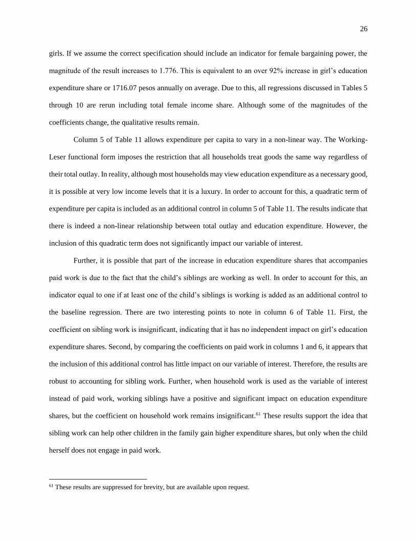
Column 5 of Table 11 allows expenditure per capita to vary in a non-linear way. The Working-

Leser functional form imposes the restriction that all households treat goods the same way regardless of

their total outlay. In reality, although most households may view education expenditure as a necessary good,

it is possible at very low income levels that it is a luxury. In order to account for this, a quadratic term of

expenditure per capita is included as an additional control in column 5 of Table 11. The results indicate that

there is indeed a non-linear relationship between total outlay and education expenditure. However, the

inclusion of this quadratic term does not significantly impact our variable of interest.

Further, it is possible that part of the increase in education expenditure shares that accompanies

paid work is due to the fact that the child’s siblings are working as well. In order to account for this, an

indicator equal to one if at least one of the child’s siblings is working is added as an additional control to

the baseline regression. There are two interesting points to note in column 6 of Table 11. First, the

coefficient on sibling work is insignificant, indicating that it has no independent impact on girl’s education

expenditure shares. Second, by comparing the coefficients on paid work in columns 1 and 6, it appears that

the inclusion of this additional control has little impact on our variable of interest. Therefore, the results are

robust to accounting for sibling work. Further, when household work is used as the variable of interest

instead of paid work, working siblings have a positive and significant impact on education expenditure

shares, but the coefficient on household work remains insignificant.61 These results support the idea that

sibling work can help other children in the family gain higher expenditure shares, but only when the child

herself does not engage in paid work.

61 These results are suppressed for brevity, but are available upon request.

27

The results presented in Table 11, show that the relationship between paid work and education

expenditure shares are robust across a variety of circumstances. Unsurprisingly, the positive relationship

between girl’s work and education expenditure shares is strongest among children residing in poorer

households in rural areas, and only holds for paid work. Additionally, the relationship seems to be driven

by an increase in expenditures that improves the quality of education over the quantity and does not appear

to negatively impact other measures of child welfare. These results are consistent with the idea that work

is not interfering with the ability to attend school, but rather it helps children earn higher education

expenditure shares in the household.

VI. Discussion

This paper has added to the literature by using a unique dataset with detailed information on work

and spending to test whether child labor adversely impacts child welfare. More specifically, the empirical

relationship between child work and education expenditure shares is explored in the context of Mexico.

The results imply that in some cases, engaging in work may actually be welfare improving for children, as

it increases their share of household resources. However, the impacts differ by characteristics of both the

child and the household. In particular the child’s gender and the type of work performed have significantly

different impacts on education expenditure shares. Further characteristics of the household, including

income, location, and female bargaining power have independent impacts as well. Overall, girls who reside

in poorer households located in rural areas see the largest benefits from paid work. Additionally, the benefit

appears to be in improvements in the quality of the girl’s educational experience as opposed to strictly

increasing their school attendance. One possible mechanism through which this occurs is that by

contributing to household income, children are rewarded with higher expenditure shares within the

household.

These results are consistent with a small literature which looks at the impact of working on

household expenditures. In particular, Moehling (2005) finds that girls who engage in work have higher

private clothing expenditures than non-working children, thus providing a benefit and an incentive to work.

28

However, they are in contrast with a large portion of the child labor literature which posits that working

can interfere with both the quantity and the quality of a child’s educational experience. Much of the popular

and economic literature also take the position that work is particularly harmful for female children. Due to

the double burden62 that female children face, both their incidence of work (Blanco Allasi, 2009) and the

actual hours they engage in work tend to be higher than their male counterparts (Kumar, 2013). Part of this

contrast may be due to the focus on the case of Mexico, where school attendance rates are known to be high

among both working and non-working children.

In fact, it is likely that the relationship varies significantly depending on the severity of the child

labor problem and the context in which it occurs. Future research should focus on poorer country contexts

and exploit information on the actual jobs children are engaged in as well as the income they bring into the

household. As the richness of household datasets improve, these tasks will become more necessary and

informative. Understanding the relationship between child labor and education expenditure in various

contexts provides new insight into the relationship between work, education, and overall investments in

children. Examining these complex relationships is essential to developing effective policy at both an

international and national level in regards to child labor and education.

This paper provides preliminary evidence that is in contrast to the traditional views of child labor.

It further provides results that are consistent with the idea that children may actually have incentives to

work. If this is the case, a new view of the child labor issue may be necessary. As Edmonds (2008) points

out, if the child plays a major role in the decision-making process, common policy responses, which include

laws banning child labor and anti-poverty policies, may not be effective. Instead, programs which directly

target the incentives of these children are more likely to decrease the number of working children,

particularly those involved in dangerous tasks.

62 This double burden is likely the result of traditional gender roles which cause females to engage in outside market

work as well as household work.

29

Table 1: Household Summary Statistics

Means: Household Characteristics

All HH

HH with

Children in

Paid Work

HH with No

Children in

Paid Work

Average Years Education of HH Head 3.94 3.49 4.00

(2.06) (1.84) (2.09)

Head Employed in Past 12 Months (%) 87.69 88.13 87.62

(32.86) (32.38) (32.94)

Female Headed HH (%) 16.94 20.52 16.41

(37.51) (40.42) (37.04)

Located in Urban Area (%) 56.96 53.92 57.40

(49.52) (49.90) (49.46)

Own House (%) 70.09 70.42 70.04

(45.79) (45.69) (45.81)

Below Median Poverty Line (%) 57.40 63.58 56.50

(49.46) (48.17) (49.58)

Annual Expend per Capita (2005 pesos) 18369.76 14674.62 18907.06

(104437.8) (49245.8) (110179)

Average HH Size 5.26 5.78 5.18

(1.81) (2.03) (1.76)

Share Males Age 0 to 4 4.01 3.58 4.07

(8.36) (7.65) (8.45)

Share Females Age 0 to 4 3.97 2.84 4.13

(8.41) (6.77) (8.61)

Share Males Age 5 to 9 9.09 8.40 9.19

(12.68) (11.87) (12.79)

Share Females Age 5 to 9 8.92 7.44 9.14

(12.32) (11.21) (12.46)

Share Males Age 10 to 14 9.22 14.47 8.46

(12.56) (13.55) (12.22)

Share Females Age 10 to 14 9.26 10.95 9.01

(12.61) (12.56) (12.60)

Share Males Age 15 to 54 22.37 21.12 22.55

(13.38) (13.93) (13.30)

Share Females Age 15 to 54 26.94 25.86 27.09

(12.35) (11.84) (12.42)

Share Males Age 55 and Over 2.75 2.32 2.81

(7.20 (6.21) (7.34)

Share Females Age 55 and Over 2.78 2.35 2.84

(7.66) (6.53) (7.80)

Observations 3915 497 3418

Households with Child Workers (%) 12.69

30

Table 2: Individual Summary Statistics

Means: Individual Characteristics

All Children Children in Paid Work

Girls Boys Girls Boys

Children in Paid Work (%) 3.73 6.79 100 100

(18.95) (25.18) (0.00) (0.00)

Paid Work Hours per Week 2.57 4.79 62.03 64.66

(15.38) (21.32) (46.46) (49.38)

Child in Household Work (%) 73.86 53.66 94.02 76.14

(43.94) (49.87) (23.79) (42.68)

Household Work Hours per Week 7.73 4.66 13.10 9.72

(10.27) (8.41) (13.18) (12.97)

Education Expenditure Budget Share (%) 1.92 1.84 2.97 1.68

(3.69) (3.10) (9.68) (2.47)

Age (Years) 10.35 10.34 12.09 12.08

(2.34) (2.36) (1.80) (1.74)

Receive Scholarship (%) 31.69 30.61 36.87 37.56

(46.53) (46.09) (48.36) (48.49)

Observations 5816 5795 217 394

31

Table 3: Baseline Results Girls age 5 to 14

Individual Child's Education Expenditure Share

(1) (2) (3) (4)

Child Engaged in Paid Work 0.885 0.898 0.961 0.933***

(0.657) (0.617) (0.618) (0.333)

Age -0.659*** -0.648*** -0.651*** -0.537**

(0.171) (0.166) (0.165) (0.212)

Age Squared 0.036*** 0.036*** 0.037*** 0.033***

(0.009) (0.008) (0.008) (0.010)

Log of HH Size -2.476*** -2.205*** -4.186***

(0.315) (0.277) (0.924)

Log Expenditures per Capita -0.997*** -1.333*** -1.930***

(0.162) (0.181) (0.123)

Share Males Age 0 to 4 0.390 0.000 0.100

(1.110) (1.049) (2.231)

Share Females Age 0 to 4 0.181 -0.400 -0.907

(1.152) (1.129) (1.987)

Share Males Age 5 to 14 -0.978 -1.405 -2.000

(1.009) (0.938) (2.293)

Share Females Age 5 to 14 -0.605 -0.977 -1.838

(0.991) (0.935) (2.015)

Share Males Age 15 to 54 0.406 0.139 0.600

(0.890) (0.891) (2.402)

Share Females Age 15 to 54 0.448 -0.007 -2.714

(1.040) (0.983) (2.096)

Share Males Age 55 and Over 0.921 1.814 1.582

(1.757) (1.741) (3.229)

HH Head Education 0.246*** -0.126

(0.038) (0.101)

HH Head Employment Status 0.071 0.599*

(0.189) (0.323)

Female Headed HH 0.384* -0.042

(0.219) (0.920)

Urban 0.713*** 0.267

(0.127) (0.559)

House Owned -0.062 0.116

(0.118) (0.196)

Child Receives Scholarship -0.002 0.014

(0.120) (0.156)

Year 2005 0.027 0.075 0.053 0.192

(0.097) (0.091) (0.090) (0.162)

Constant 4.663*** 17.852*** 19.369*** 29.406***

(0.836) (2.475) (2.373) (3.070)

Household Fixed Effects NO NO NO YES

Observations 5871 5871 5816 5816

R-squared 0.01 0.07 0.1 0.11

Number of Households 3065

Notes: Standard errors clustered by household in parentheses. * denotes significance at 10%; ** denotes

significance at 5%; *** denotes significance at 1%

32

Table 4: Baseline Results Boys Age 5 to 14

Individual Child's Education Expenditure Share

(1) (2) (3) (4)

Child Engaged in Paid Work -0.362*** -0.282** -0.158 -0.132

(0.141) (0.134) (0.129) (0.202)

Age -0.554*** -0.537*** -0.453*** -0.558***

(0.161) (0.159) (0.146) (0.163)

Age Squared 0.030*** 0.029*** 0.025*** 0.030***

(0.008) (0.008) (0.007) (0.008)

Log of HH Size -1.688*** -1.505*** -3.383***

(0.158) (0.158) (0.734)

Log Expenditures per Capita -0.476*** -0.762*** -1.015***

(0.062) (0.062) (0.102)

Share Males Age 0 to 4 -0.672 -0.912 1.257

(0.837) (0.903) (1.713)

Share Females Age 0 to 4 -0.133 -0.609 2.181

(0.849) (0.928) (1.616)

Share Males Age 5 to 14 -1.515* -1.811** 0.735

(0.779) (0.891) (1.719)

Share Females Age 5 to 14 -0.976 -1.17 1.535

(0.771) (0.941) (1.599)

Share Males Age 15 to 54 -0.059 -0.375 1.705

(0.785) (1.054) (1.775)

Share Females Age 15 to 54 -0.138 -0.506 0.065

(0.685) (0.766) (1.592)

Share Males Age 55 and Over -0.257 0.474 1.62

(0.949) (1.032) (2.341)

HH Head Education 0.196*** -0.163**

(0.033) (0.073)

HH Head Employment Status -0.143 -0.335

(0.172) (0.239)

Female Headed HH 0.118 0.029

(0.156) (0.724)

Urban 0.614*** -0.216

(0.094) (0.395)

House Owned -0.014 -0.432***

(0.097) (0.158)

Child Receives Scholarship -0.015 -0.015

(0.103) (0.119)

Year 2005 -0.133 -0.093 -0.118 0.14

(0.083) (0.081) (0.078) (0.121)

Constant 4.253*** 12.026*** 13.248*** 19.581***

(0.828) (1.366) (1.391) (2.438)

Household Fixed Effects NO NO NO YES

Observations 5839 5839 5795 5795

R-squared 0.01 0.03 0.06 0.06

Number of Households 3093

Notes: Standard errors clustered by household in parentheses. * denotes significance at 10%; **

denotes significance at 5%; *** denotes significance at 1%

33

Table 5: Exploring the Gender Differential

Individual Child's

Education Expenditure

Share

Household Child Clothing

Expenditure Share

Girls Boys Girls Boys

(1) (2) (3) (4)

Children Engaged in Paid Work -0.189 0.856***

(0.335) (0.282)

Paid Work Hours 0.072*** -0.002

(0.012) (0.007)

Paid Work Hours Squared -0.001*** 0.000

(0.000) (0.000)

Observations 5807 5787 5852 5829

R-squared 0.12 0.06 0.05 0.05

Number of Households 3065 3092 3073 3095

Notes: Standard errors clustered by household in parentheses. Results displayed in each column come from

separate regressions that also control for household and time fixed effects, the share of household member in

each age-sex category, log of total household size, log of expenditures per capita, household head's education,

employment status, and gender, a dummy equal to one if the household owns the house they reside in, a

dummy equal to one if the household is in an urban area, and a dummy equal to one if the individual receives

scholarships or money from Oportunidades for the purpose of attending school.

* denotes significance at 10%; ** denotes significance at 5%; *** denotes significance at 1%

34

Table 6: Heterogeneity in Positive Relationship for Girls

Individual Girl's Education Expenditure Share

Baseline

Above

Median

Poverty Line

Below

Median

Poverty Line

Urban Rural Girls Age

5-11

Girls Age

12-14

(1) (2) (3) (4) (5) (6) (7)

Child Engaged in Paid Work 0.933*** -0.345 1.793*** 0.504 1.347*** 1.160** 1.670

(0.333) (0.340) (0.539) (0.549) (0.410) (0.544) (1.031)

Observations 5816 2175 3641 3125 2691 3723 2093

R-squared 0.11 0.09 0.15 0.07 0.16 0.1 0.1

Number of Households 3065 1456 2005 1791 1324 2416 1738

Notes: Standard errors clustered by household in parentheses. Results displayed in each column come from separate regressions that also control for

household and time fixed effects, the share of household member in each age-sex category, log of total household size, log of expenditures per capita,

household head's education, employment status, and gender, a dummy equal to one if the household owns the house they reside in, a dummy equal to one if

the household is in an urban area, and a dummy equal to one if the individual receives scholarships or money from Oportunidades for the purpose of

attending school.

* denotes significance at 10%; ** denotes significance at 5%; *** denotes significance at 1%

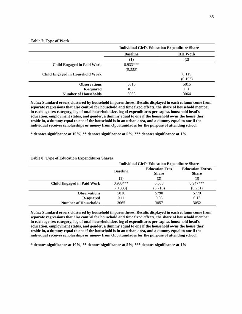
35

Table 7: Type of Work

Individual Girl's Education Expenditure Share

Baseline HH Work

(1) (2)

Child Engaged in Paid Work 0.933***

(0.333)

Child Engaged in Household Work 0.119

(0.153)

Observations 5816 5815

R-squared 0.11 0.1

Number of Households 3065 3064

Notes: Standard errors clustered by household in parentheses. Results displayed in each column come from

separate regressions that also control for household and time fixed effects, the share of household member

in each age-sex category, log of total household size, log of expenditures per capita, household head's

education, employment status, and gender, a dummy equal to one if the household owns the house they

reside in, a dummy equal to one if the household is in an urban area, and a dummy equal to one if the

individual receives scholarships or money from Oportunidades for the purpose of attending school.

* denotes significance at 10%; ** denotes significance at 5%; *** denotes significance at 1%

Table 8: Type of Education Expenditures Shares

Individual Girl's Education Expenditure Share

Baseline Education Fees

Share

Education Extras

Share

(1) (2) (3)

Child Engaged in Paid Work 0.933*** 0.088 0.947***

(0.333) (0.216) (0.231)

Observations 5816 5790 5779

R-squared 0.11 0.03 0.13

Number of Households 3065 3057 3052

Notes: Standard errors clustered by household in parentheses. Results displayed in each column come from

separate regressions that also control for household and time fixed effects, the share of household member

in each age-sex category, log of total household size, log of expenditures per capita, household head's

education, employment status, and gender, a dummy equal to one if the household owns the house they

reside in, a dummy equal to one if the household is in an urban area, and a dummy equal to one if the

individual receives scholarships or money from Oportunidades for the purpose of attending school.

* denotes significance at 10%; ** denotes significance at 5%; *** denotes significance at 1%

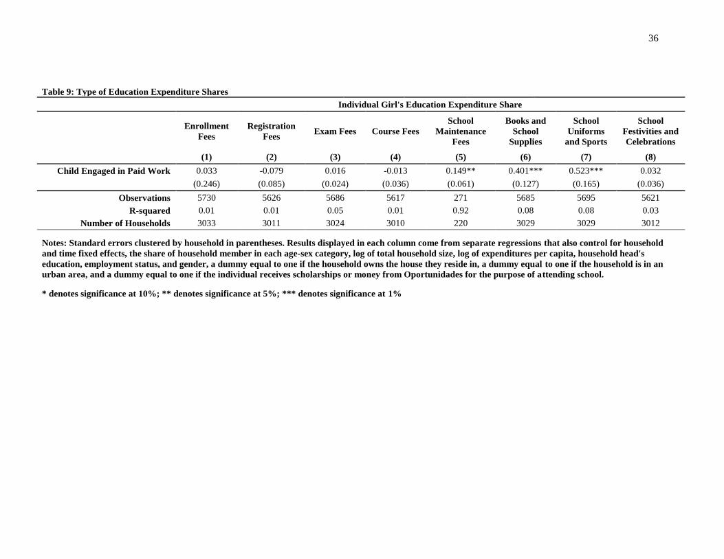
36

Table 9: Type of Education Expenditure Shares

Individual Girl's Education Expenditure Share

Enrollment

Fees

Registration

Fees Exam Fees Course Fees

School

Maintenance

Fees

Books and

School

Supplies

School

Uniforms

and Sports

School

Festivities and

Celebrations

(1) (2) (3) (4) (5) (6) (7) (8)

Child Engaged in Paid Work 0.033 -0.079 0.016 -0.013 0.149** 0.401*** 0.523*** 0.032

(0.246) (0.085) (0.024) (0.036) (0.061) (0.127) (0.165) (0.036)

Observations 5730 5626 5686 5617 271 5685 5695 5621

R-squared 0.01 0.01 0.05 0.01 0.92 0.08 0.08 0.03

Number of Households 3033 3011 3024 3010 220 3029 3029 3012

Notes: Standard errors clustered by household in parentheses. Results displayed in each column come from separate regressions that also control for household

and time fixed effects, the share of household member in each age-sex category, log of total household size, log of expenditures per capita, household head's

education, employment status, and gender, a dummy equal to one if the household owns the house they reside in, a dummy equal to one if the household is in an

urban area, and a dummy equal to one if the individual receives scholarships or money from Oportunidades for the purpose of attending school.

* denotes significance at 10%; ** denotes significance at 5%; *** denotes significance at 1%

37

Table 10: Educational Welfare Impacts for Girls

Girl's Education Outcomes

Attends

School

Hours/Day

at School

Days/Week

at School

Hours/Week

Homework

Highest

Level of

Education

Highest

Grade

Passed

Repeat

School Year

School

Disruptions

(1) (2) (3) (4) (5) (6) (7) (8)

Child Engaged in Paid Work 0.000 -0.074 -0.006 -1.232** -0.005 0.046 -0.026 -0.015

(0.002) (0.085) (0.030) (0.555) (0.032) (0.151) (0.031) (0.021)

Observations 5898 5884 5889 5833 5897 5895 5887 3943

R-squared 0.01 0.24 0.01 0.02 0.58 0.48 0.03 0.02

Number of Households 3087 3077 3083 3067 3087 3085 3086 2629

Notes: Standard errors clustered by household in parentheses. Results displayed in each column come from separate regressions that also control for household

and time fixed effects, the share of household member in each age-sex category, log of total household size, log of expenditures per capita, household head's

education, employment status, and gender, a dummy equal to one if the household owns the house they reside in, a dummy equal to one if the household is in an

urban area, and a dummy equal to one if the individual receives scholarships or money from Oportunidades for the purpose of attending school.

* denotes significance at 10%; ** denotes significance at 5%; *** denotes significance at 1%

38

Table 11: Additional Robustness Checks

Individual Girl's Education Expenditure Share

Baseline Home Owners Age Dummies Female Power Allow Income to Vary Siblings

Additional Variable Included Total Female

Income Share

Log Expenditure per

Capita Squared

Sibling Engaged in

Work

(1) (2) (3) (4) (5) (6)

Child Engaged in Paid Work 0.933*** 1.087** 0.927*** 1.776*** 0.792** 0.862**

(0.333) (0.424) (0.334) (0.572) (0.326) (0.371)

Variable 1.213** 0.545*** -0.215

(0.528) (0.049) (0.783)

Observations 5816 4215 5816 2412 5816 4493

R-squared 0.11 0.06 0.11 0.11 0.15 0.09

Number of Households 3065 2406 3065 1568 3065 2275

Notes: Standard errors clustered by household in parentheses. Results displayed in each column come from separate regressions that also control for

household and time fixed effects, the share of household member in each age-sex category, log of total household size, log of expenditures per capita,

household head's education, employment status, and gender, a dummy equal to one if the household owns the house they reside in, a dummy equal to one if

the household is in an urban area, and a dummy equal to one if the individual receives scholarships or money from Oportunidades for the purpose of

attending school.

* denotes significance at 10%; ** denotes significance at 5%; *** denotes significance at 1%

39

Chapter 2: Migration, Household Decision Making, and Child Labor

I. Introduction

According to the ILO, about 700,000 documented workers leave Indonesia each year to find

employment abroad. In addition, the number of undocumented migrants is estimated to be 2-4 times higher

(ILO, 2014). Women make up over 38% of all migrants and due to the fact that many become domestic

workers (IOM, 2013), they are seen as particularly vulnerable to exploitation (ILO, 2014). This has led the

vast majority of research on migration in Indonesia to focus on the implications for migrant workers

themselves. However, it is acknowledged that migration has consequences for both the migrant and the

family left behind (Antman, 2012b). In addition, due to the large number of female migrants in Indonesia,

it is important to understand the differential impacts on the remaining family members by the gender of the

migrant. Despite the fact that both male and female migration is common, the impacts on child labor

outcomes are not well understood.

This paper seeks to add to the literature on the impacts of migration by focusing on how migration

itself, as well as the gender of the migrants, impacts child labor and schooling outcomes. One paper that

already explicitly seeks to address these issues is Nguyen and Purnamasari (2011). The authors use the

same dataset and similar empirical strategy as this study, which will be discussed further below, to examine

how international migration and remittances in Indonesia impact the labor supply of household members

left behind and specifically child outcomes. They find that general migration decreases the overall working

hours of family members left behind, while female migration in particular reduces child labor. This paper

adds to the important contribution of Nguyen and Purnamasari (2011) by exploiting the individual level

data on children’s work and schooling, rather than relying solely on household level data. Further, this study

also empirically explores one potential mechanism through which migration could impact household and

individual outcomes, namely a change in the household decision making process.

Child labor are particularly important because despite the fact that access to education has vastly

improved in the country, many Indonesian children enter the workforce at an early age with an estimated

40

3.2 million children between the ages of 10 and 17 years currently working. Further, they often engage in

the worst forms of child labor making them particularly vulnerable to exploitation (ILO, 2014). This type

of work can have long term consequences on the individual child’s development and human capital

accumulation, while also impacting labor markets and overall economic growth in the long run.

Estimating the impact of migration on child labor is not straight forward because the migration

decision is likely endogenous to other household choices which impact resource allocation, along with work

and schooling outcomes. This often occurs because household decisions are made simultaneously, and it is

difficult to disentangle causality among contemporaneous variables. In order to address this concern, an

instrumental variables approach is applied which exploits the plausibly exogenous historical migration

networks in a potential migrant’s local community. I argue that these variables do not directly impact child

outcomes and demonstrate that they do help predict household level migration choice in Indonesia. I expand

on this strategy in Section III below.

This empirical strategy is implemented using household and individual level data from the four

rounds of the Indonesian Family Life Survey (IFLS) available in 1993, 1997, 2000, and 2007. The main

advantage of this approach is that I can exploit individual level data on children’s outcomes, rather than

looking solely at the average for any given household.1 This is important because migration can impact

different children in a household differentially, particularly based on their age and gender. In addition, this

paper exploits information on household decision making to determine one potential mechanism through

which migration has the ability to impact household choices. The main findings of this paper are that

migration has the ability to impact child labor and that these impacts differ based on the gender of the

migrant. Specifically, I find that as the total number of household migrants increases, both the probability

that a child works and his actual work hours decline. These results also suggest that the total number of

migrants has no impact on school attendance, but children in households with only female migrants are less

likely to attend school, though these results are not robust across all specifications.

1 Due to sample size issues, I was only able to exploit individual information on child work, rather than individual

information on migration choice.

41

This paper adds to the existing literature by providing insight into the complex relationships

between gender, migration, household decision making, and child labor. The remainder of this paper is

structured as follows; Section II discusses relevant background literature and the conceptual approach used

in this paper. Section III presents the empirical framework, while Section IV describes the data. Section V

presents the results regarding the impact of migration on child labor and household decision making and

discusses the robustness of these results. Section VI is left for discussion and conclusions.

II. Background

Although much of the previous literature focuses on the impacts of migration on migrants

themselves, migration can impact child labor, along with other household and individual outcomes in a

variety of ways. These impacts are also likely to differ depending on the gender of the migrant.

Many studies indicate that migration has positive impacts on child outcomes due to the increase in

remittances. Having more available income reduces the need to send a child to work, increases opportunities

for children to go to school, and improves health outcomes. For example, Yang (2008) finds that, among

other things, remittances positively impact child outcomes in the Philippines by increasing child schooling

and expenditure and decreasing child labor. Boutin (2014) further shows that increased remittances reduce

child labor in the case of Burkina Faso. This effect holds for both girls and boys, but only for younger

children within the household. Similarly, Amuedo-Dorantes and Pozo (2010) find that the impact of

remittances in the Dominican Republic varies depending on whether the household in question is a migrant

or non-migrant household. Remittances increase schooling attendance in non-migrant households, but this

effect disappears when the sample includes migrant households as well, indicating there is an overall

negative impact of migration on child schooling.

The absence of the migrant from the household can also impact child outcomes. There is evidence

that migration can negatively impact the development of children, particularly if one parent is absent for an

extended period of time. Grogger and Ronan (1995) show that long term fatherlessness in particular, results

in poorer educational attainment in single-parent families. This is supported by more recent research in

42

Albania, which indicates that parental migration, and paternal migration more specifically, results in long

term decreases in school attendance and increase in drop-outs rates (Giannelli and Mangiavacchi, 2010).

Botezat and Pfeiffer (2014) find even greater detrimental effects by showing that children in Romania with

absent parents are more likely to be mentally or physically ill.

On a different note, absence of a migrant may also cause children to incur greater responsibilities

within the household. This could result in increased household work or even entering the labor market to

earn additional income. For example, Antman (2011) finds an increase in work and a decrease in schooling

as a short run response to Mexican father’s temporary U.S. migration. On the other hand, the absence of a

large number of individuals could induce greater consequences on the overall labor market. De Paoli and

Mendola (2012) use international data to show that out-migration induces decreases in child labor through

changes in the local labor market.

Migration can also positively impact outcomes if it results in a productive accumulation of

knowledge on the part of the migrant or the household overall. For example, Hildebrant and McKenzie

(2005) find that international migration from Mexico to the US improves child health outcomes at least

partially through the increase in health knowledge that occurs with migration. Through exposure to health

practices in the US, mothers in particular gain knowledge that non-migrant household do not have access

to, resulting in lower infant mortality and higher birth weight of children.

The idea that mothers play a particularly important role in determining child outcomes manifests

in an additional channel through which migration can impact a variety of outcomes, namely by causing an

overall shift in the household decision making process. This could occur in several ways. If migration is

dominated by female migrants in a particular household, and she is the one sending remittances back to the

household, it may increase the relative bargaining power of that particular female. On the other hand, the

absence of certain household members could potentially empower remaining members, giving them more

say over both daily and long term decisions of the household. For example, Antman (2012a) indicates that

there is some evidence that women’s power increases when the husband migrates, and that this results in a

shift in resources within the household. It is generally believed that females tend to invest more in child

43

education and health outcomes. As evidence, Reggio (2011) shows that an increase in mother’s bargaining

power leads to a reduction in the amount of her child’s work. Therefore depending on how migration

influences bargaining power and subsequently household decision making, there could be several potential

impacts on child outcomes. However, the simultaneous shift in household decision making that results from

migration and its subsequent impact on children has received little attention.

Based on the previous literature, there are many potential relationships between household

migration and child outcomes. Thus this paper adds to the literature by exploring the causal effect of

migration and gender on child schooling and labor outcomes. In doing so, it accounts for the fact that

migration and absence are likely endogenous to the child labor decision. Moreover, it examines whether

evidence exists that there is a shift in decision making that occurs with migration.

III. Empirical Framework

This analysis involves empirically examining how individual child outcomes vary with the migrant

status of the household. One of the issues in estimating this relationship is that other household

characteristics may impact the migration decision, as well as child labor and educational outcomes. Part of

this is due to the fact that households that engage in migration are inherently different from those where

members do not migrate. In order to partially account for this we can reduce any bias from omitted variables

by explicitly controlling for observable characteristics of the household including household size,

composition, and total expenditure. For example, larger households with the same income may be more

likely to have a migrant, but also more likely to send a child to work. In addition, characteristics of the

household head including the head’s gender, age and education not only will impact the decision to migrate,

but also the decision to send children to work. Further, characteristics of the individual child, such as his

age and gender, will influence labor market decisions of the entire household. Failing to control for these

observable omitted variables will bias our estimates, though the direction of the bias is not entirely clear a

priori.

44

It is also important to account for any unobservable characteristics that may impact decisions within

the household. These could include the perception of sending children to work or the perceived benefits of

migration. Thus households that send children to work (and engage in migration) are inherently different

than those that do not. The estimated relationship between migration and child outcomes across households

will be biased unless these unobservable characteristics are also controlled for. In order to deal with this,

household fixed effects are applied to account for any time invariant characteristics of the household which

impact both migration and child outcomes. Thus accounting for these omitted variables and household fixed

effects, the relationship between household migration and child outcomes can be estimated as:

𝐶ℎ𝑖𝑙𝑑𝑂𝑢𝑡𝑐𝑜𝑚𝑒𝑖𝑗𝑡 = 𝛽1𝑇𝑜𝑡𝑎𝑙𝑀𝑖𝑔𝑗𝑡 + 𝑪𝒊𝒋𝒕𝜏 + 𝑯𝒋𝒕𝛿 + 𝜎𝑡 + 𝜌𝑗 + 휀𝑖𝑡 (1)

where 𝐶ℎ𝑖𝑙𝑑𝑂𝑢𝑡𝑐𝑜𝑚𝑒𝑖𝑗𝑡 is the work or education outcome for child 𝑖 in household 𝑗 at time 𝑡. This includes

an (1) indicator equal to one if the child works, (2) the total working hours of the child in the last week, and

(3) an indicator equal to one if the child currently attends school. 𝑪𝒊𝒋𝒕 is a vector of individual characteristics

including the child’s age and gender. 𝑯𝒋𝒕 is a vector of household characteristics including household size,

the total number of males and females in the household, the total number of children below the age of 15

and age 5, and the log of total household expenditures.2 In addition, this includes characteristics of the

household head such as the head’s gender, age, and educational attainment. 𝜎𝑡 are time fixed effects which

control for any macroeconomic shocks or national policies that impact all individuals and hosueholds

uniformly. 𝜌𝑗 are household fixed effects which control for any time-invariant household characteristics.

𝑇𝑜𝑡𝑎𝑙𝑀𝑖𝑔𝑗𝑡 is the variable interest and represents the total number of migrants in household j at time t. In

order to qualify as a migrant, an individual must have left the household for a time period longer than 6

months since the last interview.3

2 Expenditures have been adjusted using the Indonesian CPI from OECD.StatExtracts and are all in 2007 rupiah. 3 As a robustness check, this independent variable of interest also entered the equation as a binary variable equal to

one if the household has any migrants, zero otherwise. The first stage estimation of those results are included in

45

The above estimation will not directly give us the causal impact of migration on child labor. For

example, it is possible that factors, such as a negative income shock, could cause an individual to migrate

while also impacting the child’s decision to either attend school or go to work. Thus following other papers

in the literature (Antman, 2011; Nguyen and Purnamasari, 2011) an instrumental variables approach can be

established by proposing a set of instruments that only influence the child’s outcomes through their effect

on the migration status of the household. Equation (1) is then estimated by instrumental variables, where

the total number of migrants in a given household is estimated by the following first stage regression:

𝑇𝑜𝑡𝑎𝑙𝑀𝑖𝑔𝑗𝑡 = 𝒁𝒋𝒕𝜌 + 𝑯𝒋𝒕𝜑 + 𝜎𝑡 + є𝑖𝑡 (2)

where 𝒁𝒋𝒕 is a vector of instrumental variables excluded from Equation (1). Following Nguyen and

Purnamasari (2011) the proposed instruments include measures of historical migration networks at the

community level. In particular, they are measured as the percentage of households in the community with

migrants in 1993 and the percentage of households in the community with migrants in 1997. Since these

are historical networks, they are likely to impact the decision to migrate without directly impacting other

household decisions or child outcomes.

We expect that current migration will increase as the percentage of households with past migration

increases. This is likely due to the fact that these networks provide information that reduces the cost of

migration for an individual (Nguyen and Purnamasari, 2011). This help could come in the form of job

finding, accommodation, credit and other information (Comola and Mendola, 2014). The first stage results

of Equation (2) in Table 2 confirm that both of the historical migration rates are positive and statistically

significant determinants of current household migration status. The F-statistic for excluded instruments is

reported as 66.82. Thus living in a community with higher levels of historical migration results in

households having more current migrants.

Column (2) of Table (2), but the final stage estimations are suppressed for brevity. However those results are

consistent with the results presented here and are available upon request.

46

The main threat to identification comes from the fact that past migration networks could potentially

impact child labor directly, rather than solely through household migration status. Over identification tests

were performed and the p-values indicate that we fail to reject the null hypothesis that the excluded

instruments are exogenous. It is still possible that the exclusion restriction is not met if past migration flows

directly impact current human capital accumulation and infrastructure in these communities, which could

in turn impact household outcomes. Following Nguyen and Purnamasari (2011), in order to address this

issue, correlations between educational infrastructure, community enterprise, and historical migration rates

were explored. For instance, any additional income earned by migrants could be invested back into the

community resulting in increased access to education and thus less child labor. Since there does appear to

be correlation between some of these variables, in the final estimation I directly control for community

level characteristics. In particular, I include the number of elementary and junior high schools per capita

and an indicator of whether farming is the main enterprise of the community.

In addition to addressing the endogeneity of migration, as discussed previously, female migration

may have an independent effect on children’s outcomes relative to male migration. In order to explore this

idea, Equation (1) is modified to include an indicator equal to one if all the migrants in the household are

women and takes the following form:

𝐶ℎ𝑖𝑙𝑑𝑂𝑢𝑡𝑐𝑜𝑚𝑒𝑖𝑗𝑡 = 𝛽1𝑇𝑜𝑡𝑎𝑙𝑀𝑖𝑔𝑗𝑡 + 𝛽3𝐹𝑒𝑚𝑎𝑙𝑒𝑠𝑗𝑡 + 𝑪𝒊𝒋𝒕𝜏 + 𝑯𝒋𝒕𝛿 + 𝜎𝑡 + 𝜌𝑗 + 휀𝑖𝑡 (3)

where 𝐹𝑒𝑚𝑎𝑙𝑒𝑠𝑗𝑡 equals one if all the migrants in the household are female and zero otherwise. Thus we

are comparing households with only female migrants, to those with both male and female migrants, those

with only male migrants, and those with no migrants. In addition to the previous variables accounted for in

𝑯𝒋𝒕, this vector now also controls for community level characteristics including the number elementary

schools per capita, the number of junior high schools per capita, and an indicator equal to one if farming

is the primary enterprise of the community, zero otherwise. Equation (3) is then our equation of interest as

47

it accounts for gender differences, some of the omitted variable bias, and the endogeniety of the migration

and child work or schooling decision.

An additional part of this empirical investigation involves exploring potential mechanisms through

which migration can impact child labor. A variety of possible mechanisms have been discussed in the

previous section, but the focus of this paper will be on how migration impacts household decision making.

In order to explore this we look directly at the relationship between household decision making and the

migrants of a given household. The equation is of the following form:

𝐻𝐻𝐻𝑒𝑎𝑑𝐷𝑀𝑗𝑡 = 𝛼1 + 𝛼2𝑇𝑜𝑡𝑎𝑙𝑀𝑖𝑔𝑗𝑡 + 𝛼3𝐹𝑒𝑚𝑎𝑙𝑒𝑠𝑗𝑡 + 𝑿𝒋𝒕𝛿 + 휀𝑖𝑡 (4)

where 𝐻𝐻𝐻𝑒𝑎𝑑𝐷𝑀𝑗𝑡 is a binary indicator which measures the household head’s sole decision making

power. This variable equals 1 if the household head reports that he or she makes sole decisions regarding

household food, spending, work, social, and child investment choices. It equals zero if the decisions are

made jointly with other household members or if decisions are made independently by household members

other than the head. 𝑿𝒋𝒕 is a vector of household demographics that likely impact household decision

making including household size, the total number of males and females in the household, the total number

of children below the age of 15 and age 5, and the gender, age, and education level of the household head.

This analysis is purely reduced form and should be interpreted with caution. I am simply examining whether

households with migrants, and female migrants in particular, make decisions in different ways relative

households without migrants and those with male migrants

IV. Data

The data used in this paper come from four waves of the Indonesian Family Life Survey (IFLS1-

4) in 1993, 1997, 2000, and 2007. This survey includes nationally representative longitudinal data on the

Indonesian population with a large base of information on socioeconomic, demographic, and consumption

48

details. It covers over 30,000 individuals in 13 provinces across the country, with a re-contact rate over

90% across all waves of the survey. The major benefit is that these data include information on both child

labor and migration. Further, Indonesia is also one of the leading out-migration countries in the world.

Despite the fact that both male and female migration is common, the impacts on child labor outcomes are

not well understood. The bulk of the data comes from waves 3 and 4 of the IFLS (2000 and 2007) due to

the fact that the definitions for the variables of interest are consistent across those years of the survey. The

only information taken from waves 1 and 2 (1993 and 1997) is related to the construction of the instruments.

This includes the percentage of household in the community with migrants in those two time periods.

The child labor variables examined in this paper come from IFLS 3 and 4 and include a binary

indicator equal to one if the child has ever worked in either wage work or for the family business.4,5 In

addition, wage work and family work are also examined independently. The reason for this stems from the

fact that migration is likely to impact these two types of work in different ways. For instance, migration

may result in an increase in remittances which allows a child to attend school rather than engaging in wage

work. At the same time, the migration of an adult family member could increase the responsibilities in the

family business for an individual child. Additionally, the IFLS provides information on the actual hours

worked in these different types of employment in the past week. For the purpose of brevity, the results are

only reported using the total number of hours worked (regardless of type) in the past week as a dependent

variable. In addition to the child labor variables, we are also concerned with the relationship between

migration and schooling, as this decision is made jointly with the child work decision. Thus we examine

the impact of migration on a binary indicator equal to one if the child currently attends school and zero

otherwise.

The household decision making variable is a binary indicator which measures the household head’s

sole decision making power. This variable equals 1 if the household head reports that he makes sole

4 Working for the family business includes both farm and non-farm work. 5 In 2007, data is also available on household work, but since it is not available for 2000 as well it is excluded as an

outcome of interest in this analysis.

49

decisions on a variety of aspects. These include: the food eaten at home, routine and large household

purchases, clothing choice for the head, spouse, and children, children’s education and health, giving money

to family and friends, savings, time spent socializing, work decisions, and whether contraception is used.

This variable equals zero if the household head reports that these decisions are made jointly with other

household members or if decisions are made independently by household members other than the head.

The main independent variables of interest are the total number of migrants in a given household

and a binary indicator equal to one if all the household migrants are female. The total number of migrants

is constructed as the sum of all adult members individually reporting that they have migrated away from

home for a period of six months or longer since their last interview. In the survey it is possible to determine

whether it is the child’s parent or another household member migrating. However, due to restrictions on

sample size, this individual level data could not be utilized. It is also possible to distinguish between

domestic and international migration in the survey. Although this requires additional attention as

international and domestic migrants will inherently be different individuals, this is not of the utmost concern

in this paper. What we examine is how the actual absence from the home impacts household decision

making and child labor.6 Therefore distinguishing between international and domestic migration is less

important than determining whether or not migration occurred at all.

The other independent variable of interest is a binary indicator equal to one if all the migrants in

the household are female, and zero otherwise. Thus we are comparing households with only female

migrants to those with only male migrants, those with a mixture of male and female migrants, and those

with no migrants. The idea is that female migration in particular is altering the household structure in a way

that may result in different outcomes than if males were migrating as well. The additional community,

household, and individual level controls included in each estimation are discussed in the previous section.

Table 1 provides summary statistics for the full sample of households in Column (1) (standard deviation in

6 Additionally, the instruments did not appear as relevant for international migration as they did for migration

overall. It may be possible to explore additional instruments for international migration in the future. Similarly,

because of the individual level information it is possible to distinguish between male and female migrants offhand,

but finding suitable instruments for these two different types of migrants is a difficult task.

50

Column (2)), while Columns (3) and (4) display summary statistics for households with and without

migrants respectively.7

V. Results

a. The Impact of Migration on Child Labor

The first set of results estimates the overall impact of migration on child labor in a given household.

The results from Equations (2) and (3) on the whether a child works are presented in Table 3. In Column 1,

Equation (3) is presented only controlling for the age and gender of the child. Column (2) additionally

controls for household level attributes including demographics, household head characteristics, and the log

of total household expenditure. Column (3) further applies the instrumental variables approach discussed

in Equation (2). Column (4) includes household fixed effects, while Column (5) additionally controls for

community characteristics. The preferred specification is then Column (5) which estimates equation (3)

using instrumental variables. All results presented include year fixed effects with standard errors clustered

at the household level.8

Columns (1) through (5) indicate that regardless of the additional controls included and whether or

not instrumental variables are applied, as the total number of migrants in a household increases, the

probability that a child works declines.9 In fact, in the full specification of Column (5) having an additional

household migrant decreases the probably that a child works by .153 on average. Given that Table 1

indicates that about 4.23% of children are engaged in work, a 15 percentage point decrease in the probably

of working is extremely large in magnitude. These results also indicate that households with all female

migrants have no differential impact on child labor outcomes. Tables 4 and 5 reiterate these results by

breaking child work down into wage and family business employment. These tables show that the results

7 Table 1 indicates that 4.23% of children are engaged in work for .88 hours per work. This is the average hours

worked for all children, rather than only for those that are actually engaged in work. For those who have positive

working hours, the average is 15.671 hours of work in the past week. 8 Tables 4 through 7 are set up in the same manner. 9 The coefficient on total migrants in Column 2 is marginally significant at the 11% level.

51

in Table 3 are driven by work in the family business rather than wage work. This is somewhat surprising,

but it is possible that additional income from migrants leads to less of a need for children to work within

the family business.

Table 6 examines the impact of migration on the actual work hours of these children in the past

week. Again, Columns (1) through (5) show that migration decreases the total number of hours children are

engaged in work, while female migration does not have a differential impact. The coefficient in Column

(5) indicates that an additional migrant decreases child work hours in the last week by 5.399. This supports

the results found in Tables 3 and 5 above. Thus migration decreases both the probability that a child works

and the actual hours the child engages in work.

Lastly, we also examine the impact of migration and gender on schooling outcomes. Table 7 shows

the impacts on whether or not a specific child currently attends school. There does not appear to be any

impact of migration on child attendance, but in households with only female migrants, children are less

likely to attend school. Column (3) indicates that in households with only female migrants child attendance

falls by .041 relative to those with male migrants or no migrants at all. Given that 88.2% of these children

currently attend school, this translates into a 4.6% decline in the probably that a child currently attends

school. This result is not surprising given the fact that females and mothers in particular are known to invest

more in children’s education and development than their male counterparts. Thus when females are absent

from the household for extended periods of time, there may be less focus on making sure children attend

school than there would be in their presence. However, these results do not hold up once household fixed

effects and community characteristics are controlled for. Thus we cannot read too much into the results in

Table 7.

These results contrast with those of Nguyen and Purnamasari (2011) who find no impact of migrant

households on the total number of children in school or engaged in work, but a negative significant

relationship between female migration and child labor in the same context. This may speak to the

importance of using individual level data for this type of analysis. These results are consistent with the idea

that migration actually improves child outcomes. There are several mechanisms through which this could

52

occur. Although this is a reduced form estimation and we cannot directly tease out the exact mechanisms

at play, the next section seeks to explore one potential way through which migration can impact child

outcomes.

b. The Impact of Migration on Household Decision Making

The results in the sub-section above indicate that both the total number of migrants and having only

female migrants can independently impact child labor. One way through which this may arise is that as

individuals leave the household, the way household decision making occurs changes. Ideally we would like

to examine household decision making within the same household when the migrant is present and when

the migrant is away. Although we cannot test this directly due to data constraints, we can examine whether

households with migrants, and female migrants in particular, make decisions in different ways relative to

households without migrants and those with some male migrants. The results from Equation (4) are

presented in Table 8. Column (1) looks solely at the correlation between the household head decision

making variable and the migration variables. Column (2) includes additional demographic controls that

could impact household decision making, while Column (3) additionally controls for characteristics of the

household head. Column (4) is the preferred specification and applies the instrumental variables approach

of Equation (2).

Columns (1) through (4) of Table 8 show that the total number of migrants and having only female

migrants both independently impact decision making in the household. As expected, as the total number of

household migrants increases, the sole decision making power of the household head increases as well. This

makes logical sense as when household members are absent for an extended period of time, they will have

less control over the daily decisions made within the household, automatically giving more power to the

household head. What is more surprising and interesting is the result for households with only female

migrants. These results indicate that relative to situations with male migrants or no migrants, heads in

households with only female migrants make less independent decisions. Although surprising at first, what

this may reflect is that as female household members migrate, and in turn contribute more income to the

53

household in the form of remittances, their ability to make household decisions increases. This increase in

power for female household members then results in a decrease in the sole decision making by household

heads.

c. Robustness

In order to test the robustness of these results several additional adjustments were made to the

preferred specification. First, the total number of migrants in a given household was substituted with an

indicator equal to one if any household member is considered a migrant. Although the total number of

migrants is preferred due to the fact that households with more than one migrant will react differently from

those with a single migrant, this type of analysis gets more at the idea that migrant households are especially

distinct from non-migrant households. The results for the first stage using this indicator are presented in

Column (2) of Table (2). Although there are slight differences in the magnitude of the coefficients relative

to using the total number of household migrants, there is little difference qualitatively. Further, although

the final results are omitted for brevity, the final stage estimation remains similar.

In addition, the final stage of the analysis was estimated separately for the years 2000 and 2007.

Due to the Indonesian crisis in 1998 which encompassed economic and political turmoil, in addition to the

1997 drought, it is possible that households were still recovering and acting out of character in the 2000

survey round. Therefore, 2007 may be a better estimate of the true relationship between migration,

household decision making, and child labor. Again, these results confirm that the relationships appear

consistent across time. These results are omitted for brevity, but are available upon request.

d. Potential Heterogeneities

In addition, it is possible that the impact on children will differ substantially based on the child’s

gender and age. In order to explore this, the sample was first split by gender and the preferred specification

was run separately for female and male children. The idea here is that both the gender of the child and the

gender of the migrant may impact how children are affected. Female children are less likely to work overall

54

(at least outside of the household) and female household members may favor female children when making

household decisions. Similarly, it is possible that a pro-male bias exists where male children are always

favored. Surprisingly, there doesn’t appear to be much difference in outcomes across genders.

The sample was also split and run for children between the age of 5-9 and 10-15 independently.

Older children are more likely to work overall, but also more likely to take over any household

responsibilities in the absence adult household members. Therefore, older children may be differentially

impacted relative to younger children with less responsibility. However, the results show little difference

across the age of the child. These results are all omitted for brevity, but are available upon request. They

may indicate that migration impacts all children in similar ways, but it is also possible that the migration

data needs to be disaggregated in order to see the full effect. These sorts of heterogeneities deserve further

attention in future research.

VI. Conclusions

This paper contributes to the literature on the differential impact of migration by male and female

household members on household decision making and child labor. Using household and individual level

data from four rounds of the Indonesian Family Life Survey and exploiting an instrumental variables

approach, we show that migration causally impacts child labor and that some of these impacts differ based

on the gender of the migrant. Specifically, we find that as the total number of household migrants increases,

both the probability that a child works and his actual work hours decline. On the other hand, the total number

of migrants has no impact on school attendance, but children in households with only female migrants are

less likely to attend school, though the latter result is not robust across all specifications.

As discussed, the impact of migration on child labor could occur through many potential channels,

but this paper has provided evidence that migration does appear to shift the household decision making

process. In particular, as the total number of migrants increases, the sole decision making power of the

household head increases. In contrast the sole decision making power of the household head is lower in

households with only female migrants than in households with male or no migrants.

55

This paper adds to multiple sets of literature by examining the interaction of migration, gender,

household decision making, and child labor. Exploring these relationships provides insight into the

complicated dynamic of household decision making, while also exposing an additional channel through

which the child labor decision is made. Future research should seek to exploit the individual level

information on both child labor and migration to get a clearer picture of how these decisions are made.

56

Table 1

Descriptive Statistics

Variable Mean Standard deviation

HH with migrants

HH without migrants

Child outcomes

Child Worker 0.042 (.201) 0.028 0.047

Child Wage Worker 0.009 (0.094) 0.007 0.010

Child Family Business Worker 0.036 (0.186) 0.023 0.040

Child Work Hours 0.880 (5.768) 0.722 0.930

Child Currently Attends School 0.882 (.323) 0.866 0.887

Household Demographics

HH Size 6.760 (2.859) 6.743 6.765

Total Males 3.250 (1.718) 3.239 3.234

Total Females 3.345 (1.729) 3.38 3.334

Children Under 15 2.596 (1.279) 2.623 2.588

Children Under 5 0.655 (.749) 0.737 0.629

Male Headed HH 0.881 (.323) 0.899 0.876

Age of HH Head 43.964 (10.808) 42.609 44.397

Education of HH Head 4.826 (2.714) 5.161 4.718

Log of Total HH Expenditure 16.504 (.889) 16.67 16.451

Migration

Total HH Migrants 0.342 (.671) 1 0

HH with only Female Migrants 0.088 (.283) 0.363 0

HH with only Male Migrants 0.069 (.253) 0.285 0

24.22% 75.78%

Observations 12613 3055 9558

57

Table 2

First Stage: Determinants of Household Migrants

Total Household Migrants HH With Migrants

OLS OLS

(1) (2)

HH Size -0.0231 -0.0140

(0.165) (0.177)

Total Males in HH 0.0257 0.0147

(0.172) (0.200)

Total Females in HH 0.03110* 0.02112*

(0.092) (0.064)

Total Children Under 15 -0.02302* -0.02357***

(0.057) (0.001)

Total Children Under 5 0.05361*** 0.04352***

0.000 0.000

Male HH Head 0.06856*** 0.0094

(0.001) (0.547)

Age of HH Head -0.00342*** -0.00267***

0.000 0.000

Education of HH Head 0.00758** 0.00486**

(0.015) (0.014)

Log of Total HH Expenditure 0.08387*** 0.04657***

0.000 0.000

Percent of Community HH with Migrants in 1997 0.27238*** 0.14242***

0.000 (0.001)

Percent of Community HH with Migrants in 1993 0.19310*** 0.12474***

(0.001) (0.002)

Constant -1.40779*** -0.65697***

0.000 0.000

Year fixed effects YES YES

Number of observations 12823 12823

R-squared 0.039 0.038

F-statistic for excluded instruments 66.82 52.84

Notes: Standard errors clustered by household are in parentheses.

Asterisks denote significance: * significant at 10%; ** significant at 5%; *** significant at 1%

58

Table 3

Effect of Migration on Child Labor

Child Worker

OLS OLS IV IV IV

(1) (2) (3) (4) (5)

Total HH Migrants -0.00703*** -0.00454* -0.11041** -0.17176*** -0.15347**

(0.002) (0.003) (0.011) (0.064) (0.070)

HH with only Female Migrants 0.00276 -0.00092 -0.0029 -0.01603 -0.01555

(0.006) (0.006) (0.614) (0.015) (0.017)

Age 0.01437*** 0.01403*** 0.01377*** 0.01450*** 0.01498***

(0.001) (0.001) 0.000 (0.001) (0.001)

Female -0.00524 -0.00813** -0.00559 -0.00759 -0.00869

(0.003) (0.004) (0.152) (0.005) (0.006)

HH Size 0.00885 0.00832 -0.00147 -0.00161

(0.006) (0.182) (0.009) (0.011)

Total Males in HH -0.00914 -0.00786 0.01006 0.0101

(0.006) (0.234) (0.010) (0.011)

Total Females in HH -0.00815 -0.00715 -0.00282 -0.00364

(0.006) (0.286) (0.009) (0.010)

Total Children Under 15 0.00502* 0.00279 -0.01855*** -0.01524***

(0.003) (0.319) (0.005) (0.006)

Total Children Under 5 -0.00001 0.00516 0.02448*** 0.01904**

(0.003) (0.221) (0.007) (0.008)

Male HH Head -0.00473 0.00086 -0.0206 -0.01839

(0.007) (0.908) (0.017) (0.019)

Age of HH Head 0.000 -0.00041 -0.00190*** -0.00194***

(0.000) (0.137) (0.001) (0.001)

Education of HH Head -0.00426*** -0.00328*** -0.00442** -0.00524**

(0.001) 0.000 (0.002) (0.002)

Log of Total HH Expenditure -0.00347 0.00697 0.00949 0.00472

(0.002) (0.143) (0.008) (0.009)

Constant -0.11503*** -0.0461 -0.16779*** -0.07195 -0.02562

(0.006) (0.041) (0.007) (0.126) (0.143)

Year fixed effects YES YES YES YES YES

HH fixed effects NO NO NO YES YES

Community Controls NO NO NO NO YES

Number of observations 14447 13636 12823 12823 10685

R-squared 0.06 0.06 0.062 0.09 0.1

Notes: Standard errors clustered by household are in parentheses. Community controls include an indicator equal to one if the primary enterprise in the community is farming, the number of elementary schools per capita in the community, and the number of junior high school per capita in the community.

Asterisks denote significance: * significant at 10%; ** significant at 5%; *** significant at 1%

59

Table 4

Effect of Migration on Child Labor

Child Wage Worker

OLS OLS IV IV IV

(1) (2) (3) (4) (5)

Total HH Migrants -0.0013 -0.0006 -0.0136 -0.05003* -0.0465

(0.001) (0.001) (0.408) (0.030) (0.034)

HH with only Female Migrants 0.00078 0.00039 0.00034 0.0004 0.00086

(0.003) (0.003) (0.911) (0.007) (0.008)

Age 0.00326*** 0.00323*** 0.00333*** 0.00320*** 0.00340***

(0.000) (0.000) 0.000 (0.000) (0.000)

Female -0.00158 -0.00363** -0.00321* -0.00445* -0.00436

(0.001) (0.002) (0.088) (0.002) (0.003)

HH Size 0.0023 0.00242 -0.0031 -0.00474

(0.002) (0.365) (0.004) (0.005)

Total Males in HH -0.00316 -0.00326 0.00162 0.0025

(0.003) (0.265) (0.005) (0.005)

Total Females in HH -0.00178 -0.00186 -0.00099 -0.00116

(0.003) (0.520) (0.004) (0.005)

Total Children Under 15 0.0011 0.00104 0.00444* 0.00597**

(0.001) (0.435) (0.002) (0.003)

Total Children Under 5 0.00114 0.00181 0.00734** 0.00716*

(0.001) (0.305) (0.003) (0.004)

Male HH Head -0.00148 -0.00046 0.00485 0.0047

(0.003) (0.888) (0.008) (0.009)

Age of HH Head 0.00003 -0.00001 -0.00066** -0.00068*

(0.000) (0.945) (0.000) (0.000)

Education of HH Head -0.00167*** -0.00145*** -0.00196* -0.00212*

(0.000) (0.001) (0.001) (0.001)

Log of Total HH Expenditure -0.00063 0.00071 0.00815** 0.00834*

(0.001) (0.719) (0.004) (0.005)

Constant -0.02315*** -0.00652 -0.02546 -0.10304* -0.10806

(0.003) (0.014) (0.305) (0.060) (0.069)

Year fixed effects YES YES YES YES YES

HH fixed effects NO NO NO YES YES

Community Controls NO NO NO NO YES

Number of observations 14341 13535 12722 12722 10594

R-squared 0.01 0.01 0.014 0.02 0.02 Notes: Standard errors clustered by household are in parentheses. Community controls include an indicator equal to one if the primary enterprise in the community is farming, the number of elementary schools per capita in the community, and the number of junior high school per capita in the community.

Asterisks denote significance: * significant at 10%; ** significant at 5%; *** significant at 1%

60

Table 5

Effect of Migration on Child Labor

Child Family Business Worker

OLS OLS IV IV IV

(1) (2) (3) (4) (5)

Total HH Migrants -0.00567** -0.0038 -0.09276** -0.13591** -0.12412*

(0.002) (0.002) (0.024) (0.060) (0.066)

HH with only Female Migrants 0.00269 -0.0008 -0.00252 -0.01841 -0.01816

(0.005) (0.005) (0.634) (0.014) (0.016)

Age 0.01241*** 0.01213*** 0.01177*** 0.01267*** 0.01295***

(0.001) (0.001) 0.000 (0.001) (0.001)

Female -0.00443 -0.00597 -0.00365 -0.00337 -0.00376

(0.003) (0.004) (0.325) (0.005) (0.006)

HH Size 0.00678 0.00632 0.00206 0.00405

(0.005) (0.279) (0.008) (0.010)

Total Males in HH -0.00659 -0.00541 0.00994 0.00966

(0.006) (0.380) (0.009) (0.010)

Total Females in HH -0.00664 -0.00582 -0.00273 -0.00327

(0.006) (0.352) (0.009) (0.009)

Total Children Under 15 0.00417* 0.0022 -0.02200*** -0.02058***

(0.003) (0.415) (0.005) (0.005)

Total Children Under 5 -0.00057 0.00373 0.01945*** 0.01395*

(0.003) (0.358) (0.007) (0.007)

Male HH Head -0.00176 0.00243 -0.02306 -0.0197

(0.006) (0.736) (0.017) (0.018)

Age of HH Head 0.00003 -0.00032 -0.00139** -0.00145**

(0.000) (0.216) (0.001) (0.001)

Education of HH Head -0.00295*** -0.00219*** -0.00183 -0.00226

(0.001) (0.009) (0.002) (0.002)

Log of Total HH Expenditure -0.00354 0.00526 0.00249 -0.00278

(0.002) (0.240) (0.008) (0.009)

Constant -0.09967*** -0.0376 -0.13800** 0.00309 0.05329

(0.006) (0.040) (0.021) (0.120) (0.134)

Year fixed effects YES YES YES YES YES

HH fixed effects NO NO NO YES YES

Community Controls NO NO NO NO YES

Number of observations 13987 13199 12388 12388 10282

R-squared 0.05 0.05 0.053 0.08 0.09 Notes: Standard errors clustered by household are in parentheses. Community controls include an indicator equal to one if the primary enterprise in the community is farming, the number of elementary schools per capita in the community, and the number of junior high school per capita in the community.

Asterisks denote significance: * significant at 10%; ** significant at 5%; *** significant at 1%

61

Table 6

Effect of Migration on Child Labor

Child Work Hours Last Week

OLS OLS IV IV IV

(1) (2) (3) (4) (5)

Total HH Migrants -0.17452*** -0.15394** -1.31587** -4.79252** -5.39868**

(0.059) (0.061) (0.036) (1.972) (2.206)

HH with only Female Migrants 0.11432 0.16982 0.09059 -0.93388** -0.72875

(0.172) (0.206) (0.672) (0.461) (0.542)

Age 0.32308*** 0.31869*** 0.33271*** 0.35617*** 0.37848***

(0.022) (0.022) 0.000 (0.026) (0.030)

Female -0.00432 0.01942 0.04167 -0.06695 0.00351

(0.099) (0.111) (0.721) (0.162) (0.186)

HH Size 0.03885 0.01125 -0.09721 0.04133

(0.081) (0.895) (0.277) (0.340)

Total Males in HH -0.06758 -0.03578 0.27469 0.20975

(0.098) (0.729) (0.305) (0.341)

Total Females in HH -0.07321 -0.0429 0.14371 -0.02321

(0.096) (0.669) (0.284) (0.319)

Total Children Under 15 0.15100** 0.12702* -0.02943 -0.05392

(0.064) (0.063) (0.153) (0.180)

Total Children Under 5 -0.02682 0.04185 0.19235 0.24194

(0.081) (0.659) (0.219) (0.250)

Male HH Head -0.31404 -0.27193 0.19184 0.45769

(0.217) (0.244) (0.540) (0.605)

Age of HH Head -0.00314 -0.00761 0.02417 0.00749

(0.006) (0.272) (0.021) (0.023)

Education of HH Head -0.10894*** -0.10161*** 0.03929 0.0272

(0.024) 0.000 (0.068) (0.078)

Log of Total HH Expenditure 0.08506 0.20524** 0.42437 0.53125*

(0.074) (0.049) (0.259) (0.294)

Constant -1.56251*** -2.19880* -3.73636** -8.88469** -9.65512**

(0.165) (1.144) (0.012) (3.907) (4.515)

Year fixed effects YES YES YES YES YES

HH fixed effects NO NO NO YES YES

Community Controls NO NO NO NO YES

Number of observations 14462 13652 12838 12838 10701

R-squared 0.03 0.04 0.037 0.03 0.03 Notes: Standard errors clustered by household are in parentheses. Community controls include an indicator equal to one if the primary enterprise in the community is farming, the number of elementary schools per capita in the community, and the number of junior high school per capita in the community.

Asterisks denote significance: * significant at 10%; ** significant at 5%; *** significant at 1%

62

Table 7

Effect of Migration on Child Education

Child Currently Attend School

OLS OLS IV IV IV

(1) (2) (3) (4) (5)

Total HH Migrants 0.0042 0.0028 -0.0165 -0.1574 -0.1462

(0.003) (0.003) (0.640) (0.099) (0.103)

HH with only Female Migrants -0.05126*** -0.04629*** -0.04148*** -0.00416 -0.0037

(0.008) (0.008) 0.000 (0.022) (0.024)

Age 0.07055*** 0.06292*** 0.06110*** 0.06356*** 0.06109***

(0.001) (0.001) 0.000 (0.001) (0.001)

Female 0.00656 0.01154** 0.01281** 0.00929 0.00404

(0.005) (0.006) (0.027) (0.007) (0.008)

HH Size 0.00208 0.00143 0.03680*** 0.03654**

(0.004) (0.763) (0.014) (0.016)

Total Males in HH -0.00584 -0.00516 0.0068 0.00984

(0.005) (0.340) (0.015) (0.016)

Total Females in HH -0.00447 -0.00403 0.02096 0.02854**

(0.005) (0.451) (0.014) (0.014)

Total Children Under 15 0.03294*** 0.03301*** -0.08426*** -0.08333***

(0.003) 0.000 (0.008) (0.008)

Total Children Under 5 -0.09927*** -0.09703*** -0.07598*** -0.08759***

(0.005) 0.000 (0.010) (0.011)

Male HH Head 0.00054 0.00519 0.01977 0.01459

(0.008) (0.545) (0.026) (0.027)

Age of HH Head -0.00002 0.00001 -0.00144 -0.001

(0.000) (0.961) (0.001) (0.001)

Education of HH Head 0.00956*** 0.00961*** 0.00324 0.00271

(0.001) 0.000 (0.003) (0.004)

Log of Total HH Expenditure 0.01721*** 0.01819*** 0.00982 0.00321

(0.003) 0.000 (0.013) (0.014)

Constant 0.26101*** 0.00127 0.00178 0.26422 0.36883*

(0.007) (0.042) (0.977) (0.193) (0.208)

Year fixed effects YES YES YES YES YES

HH fixed effects NO NO NO YES YES

Community Controls NO NO NO NO YES

Number of observations 18381 17283 16110 16110 12923

R-squared 0.52 0.54 0.532 0.43 0.43 Notes: Standard errors clustered by household are in parentheses. Community controls include an indicator equal to one if the primary enterprise in the community is farming, the number of elementary schools per capita in the community, and the number of junior high school per capita in the community.

Asterisks denote significance: * significant at 10%; ** significant at 5%; *** significant at 1%

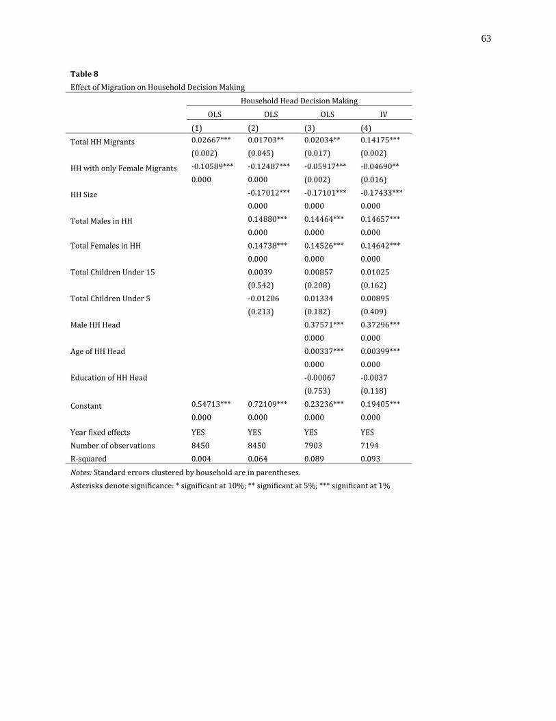
63

Table 8

Effect of Migration on Household Decision Making

Household Head Decision Making

OLS OLS OLS IV

(1) (2) (3) (4)

Total HH Migrants 0.02667*** 0.01703** 0.02034** 0.14175***

(0.002) (0.045) (0.017) (0.002)

HH with only Female Migrants -0.10589*** -0.12487*** -0.05917*** -0.04690**

0.000 0.000 (0.002) (0.016)

HH Size -0.17012*** -0.17101*** -0.17433***

0.000 0.000 0.000

Total Males in HH 0.14880*** 0.14464*** 0.14657***

0.000 0.000 0.000

Total Females in HH 0.14738*** 0.14526*** 0.14642***

0.000 0.000 0.000

Total Children Under 15 0.0039 0.00857 0.01025

(0.542) (0.208) (0.162)

Total Children Under 5 -0.01206 0.01334 0.00895

(0.213) (0.182) (0.409)

Male HH Head 0.37571*** 0.37296***

0.000 0.000

Age of HH Head 0.00337*** 0.00399***

0.000 0.000

Education of HH Head -0.00067 -0.0037

(0.753) (0.118)

Constant 0.54713*** 0.72109*** 0.23236*** 0.19405***

0.000 0.000 0.000 0.000

Year fixed effects YES YES YES YES

Number of observations 8450 8450 7903 7194

R-squared 0.004 0.064 0.089 0.093

Notes: Standard errors clustered by household are in parentheses.

Asterisks denote significance: * significant at 10%; ** significant at 5%; *** significant at 1%

64

Chapter 3: Does Political Reservation Affect Child Labor? Evidence

from India (with Nishith Prakash)

I. Introduction

Historical discrimination in India has led to the emergence of disadvantaged groups which are

excluded from accessing opportunities and resources, resulting in their under-representation in politics,

public sector jobs, and other areas. In response, the Indian Constitution mandates that a certain share of

seats be reserved in the state legislative assemblies and the national parliament (i.e. the Lok Sabha or the

lower house) for two minority groups, namely Scheduled Castes (SCs) and Scheduled Tribes (STs). In

addition, the federal and state government use policy initiatives to improve the well-being of SCs and STs.

Previous studies have estimated the causal impact of political reservation for minorities on a variety of

policy outcomes including welfare spending, land reforms, employment, and poverty. However, the

majority of these studies look at aggregate outcomes at the state or district level and find mixed results. A

related paper by Chin and Prakash (2011) finds that political reservation for STs reduces aggregate poverty

in rural India, while political reservation for SCs has no impact. Despite the strong link between poverty

and child labor, it remains unclear how these aggregate impacts will translate into household level

outcomes. To the best of our knowledge there is no empirical evidence on how these affirmative action

policies impact the well-being of minority groups and the overall population. This paper adds to the growing

literature on the impacts of affirmative action policies by examining the effect of political reservation on

child labor at the household level in India.1

Child labor is a particularly relevant measure of well-being because despite efforts to prevent it,

the 2001 national census estimates that there are 12.6 million children working in India. Further, child labor

rates are known to be especially high for the minority groups of interest in this paper. Thus child labor is

likely to be an issue of concern for these groups and one that state elected representatives can directly

1 It should be noted here that we are assuming a decrease in paid work by children is welfare improving for these

households. On the contrary, it could actually be the case that an increase in child labor is a positive outcome in that

it could represent a shift from bonded labor to paid work.

65

address. Additionally, because of the complex social relationships in Indian society, minority representation

for SCs and STs may actually impact child labor in different ways.

However, estimating the impact of political reservation for minorities on child labor is difficult

because political reservation is likely endogenous to the outcome variables of interest. This could occur

because the percentage of minorities elected in certain areas or states may vary in ways that also impact the

magnitude and intensity of child labor, along with other socioeconomic outcomes. In order to address

endogeneity concerns we use the empirical strategy established in Pande (2003) and implemented in Chin

and Prakash (2011), which involves isolating the effect of other omitted variables. However, it is necessary

to point out one important difference from their identification strategy. Pande (2003) and Chin and Prakash

(2011) are able to exploit the within-state cross-time variation in the share of seats reserved for minorities

because they are using data from 1960--2000. However, we are limited by the availability of only two

rounds of nationally representative rural household data from 1982 and 1999. The main advantage of this

data is our ability to examine group specific outcomes on child labor at the household level. There are no

household surveys that include child labor outcomes dating back to the 1960s. Due to this, we can only

exploit the across-state variation in the share of seats reserved. We further elaborate on this strategy in

Section III.

In the case of India, according to the Constitution, the share of seats reserved for the two minority

groups is proportional to, and solely determined by, their share of the state population in the last preceding

census. One implication of this rule is that minority population share is correlated with minority political

reservation, but it may also be correlated with other characteristics that impact child labor. For instance,

minority population share could impact how resources are allocated within and across states and therefore

how effective policy is in quelling the negative impacts that lead to high child labor prevalence. However,

several institutional features allow us to address this issue by directly controlling for both the current and

last preceding census minority population share.

The empirical strategy is implemented using state and household level data from multiple sources

on fifteen major Indian states in 1982 and 1999. Our main findings indicate that at the household level, ST

66

reservation decreases child labor, while SC reservation actually increases the total number of children

working. We examine these impacts on the general as well as the disadvantaged group population

independently, and also explore potential explanations for the differential impact of SC and ST political

reservation.2

Political reservation policies for disadvantaged minorities have the potential to affect policy

outcomes as a quarter of all legislators in India come from reserved jurisdictions. However, the impact of

an increase in minority representation on the well-being of the minority groups and the overall population

is an empirical question. It is possible that these policies benefit minorities and non-minorities by increasing

opportunities and available resources. On the other hand, elite capture could occur or any benefits to

minority group members could come at the cost of non-minorities. Past empirical literature on the impacts

of state level political reservation provides multiple channels through which the shift in resources due to

political reservation could impact well-being. For example, Pande (2003) uses data from sixteen major

Indian states from 1960-1992, to estimate the impact of SC and ST political reservation on general and

targeted government policies separately.3 She finds that ST reservation increases spending on ST welfare

programs and lowers educational and overall government spending, while SC reservation increases the

number of state government jobs reserved for minorities. Despite these results, Pande (2003) concludes that

it is still unknown whether the redistribution in spending and job quotas enhances the well-being of the

minority groups or the general population. This is particularly important for our present study as increased

welfare spending could result in improved circumstances at the household level leading to a potential

decline in child labor. On the other hand, if the increased spending results in a higher rate of economic

activity or trade, an increase in demand could cause child labor prevalence to rise. Similarly, if elite capture

occurs or a decrease in education spending results in the lowering of the availability or quality of education,

households may actually find themselves in worse situations where child labor is more necessary.

2 Here disadvantaged groups are defined as Scheduled Castes, Scheduled Tribes, and Other Backward Class. 3 In Pande (2003) general government policies include total per capita state spending, total education spending, and

whether or not a land reform act occurs. Targeted policies include the fraction of government spending going

towards SC and ST welfare programs, along with job quotas for those groups.

67

In a related paper by Krishnan (2007) the importance of access to education is further exhibited.

Krishnan (2007) finds that SC legislators improve access to primary schools, which benefit both SC and

non-SC groups, while ST legislators perform similarly to legislators in unreserved constituencies.4 These

results confirm the idea that SC and ST reservation may impact child labor in different ways and provide

an additional channel through which that may occur.

Further, in order to address well-being at the aggregate level, Chin and Prakash (2011) look at the

impacts of minority representation on poverty outcomes, finding that increasing the share of minority seats

reserved for STs reduces overall poverty, while SC reservation has no impact on poverty. The child labor

literature has established a strong link between poverty and child labor. In particular, decreases in poverty

(or increases in income) is one of the most important mechanisms to improving child labor outcomes.

However, this relationship is by no means a requirement. It is also possible that any decrease in poverty

could actually be a direct result of children entering the labor market in order to help reach subsistence

consumption. To clarify, the results in Chin and Prakash are for overall poverty rates in the general

population. Households that tend to send children to work are extremely poor and are not necessarily the

same households which see improvements in poverty with ST reservation. Improvements in poverty rates

are more likely to occur near the poverty line than in households far below it. Thus it remains unclear how

these aggregate impacts will translate into household level outcomes.5

4 Krishnan (2007) is examining whether districts represented by more minority legislators provide different public

goods relative to non-minority representatives. In this case public goods refer to availability of educational and

health facilities. She concludes that there is no evidence to support the theory that political reservation negatively

impacts electoral competition or the quality of legislators. 5 Several studies have also explored the impact of women's and local level SC and ST reservation. For example,

Chattopadhyay and Duflo (2004) find that women representatives in the Gram Panchayat (bottom tier of local

government) tend to shift spending towards the allocation of local public goods, such as drinking water and roads.

On the other hand, Bardhan et al. (2010) find no significant effects of women pradhan (mayor) reservations on the

same public policy aspects in West Bengal. Mookherjee (2012) provides a summary of these, along with similar

papers, and concludes that it is still unclear if women reservations will have long run impacts on policies. In the case

of SC and ST reservation at the village level, SC and ST pradhans increase the probability that households in that

village have a toilet, electricity connection, and private waterline (Besley, Pande, Rahman and Rao, 2004), as well as

increase the benefits from the local government for housing construction and improvements (Bardhan, Mookherjee

and Parra Torrado, 2010). Similarly, having an SC pradhan increases public goods to areas where SCs are

concentrated (Duflo, Fischer and Chattopadhyay, 2008).}

68

Previous literature has focused on how state level political reservation impacts aggregate policy

outcomes and provides several potential links between reservation and well-being. We are not aware of any

paper that examines the effect of political reservation for minorities on micro-level well-being outcomes,

nor more specifically on child labor. This paper adds to the existing literature on mandated affirmative

action policies by exploring the impacts of political reservation on child labor at the household level.

Moreover, we examine group specific and general population child labor outcomes separately, while also

allowing for differential impacts across gender.

The remainder of this paper proceeds as follows: Section II discusses the background on political

reservation policies and the prevalence of child labor among minorities. Section III presents the empirical

framework and Section IV describes the data. Section V reports the main empirical results, while Section

VI discusses some robustness checks. Section VII then describes the results on the heterogeneous effects

of political reservation for minorities. Section VIII concludes.

II. Background

a. Political Reservation in State Legislative Assemblies in India

This paper focuses on two specific minority groups, SCs and STs, who make up 16.6% and 8.6%

of the population respectively.6,7 Both of these groups have been historically discriminated against and

prevented from engaging in opportunities or claiming rights that could improve their status in Indian

society. Much of this stems from discrimination in the Hindu caste system which determined that SC

members took menial jobs and were restricted from owning assets. Similarly, geographic isolation and

reliance on subsistence agricultural led to widespread poverty among STs (Pande, 2003).

6 These estimates are based on the 2011 Census data.} SCs are those groups with low social and ritual standing in

the Hindu caste hierarchy, while STs are groups identified by their tribal culture, geographic isolation, and linguistic

characteristics. These groups were formally referred to as untouchables or backward castes. 7 The Indian Constitution, specifically the Schedule Castes and Scheduled Tribe Order of 1950, stipulates which

groups are considered SCs and STs. Further, the SC and ST Orders Act of 1976 requires that SC and ST definitions

be uniform across all states.

69

In order to correct this historical discrimination, India has a long history of aggressive and

mandated affirmative action policies aimed at increasing opportunities for disadvantaged groups in

education, public sector employment and political reservation. The Constitution, effective January 26, 1950,

requires representation for SCs and STs in the lower house of Parliament (Lok Sabha) and state legislative

assemblies.8 More specifically, Article 332 of the Indian Constitution establishes that the number of seats

reserved for SCs and STs in the state legislative assemblies is determined by the share of that group's total

state population in the last preceding census. Thus the primary source of variation is the arrival of the new

census population data.9

Upon the arrival of new census figures, the Delimitation Commission is then responsible for

revising the number of seats reserved in each state for SCs and STs, along with designating the specific

constituencies in which they are reserved.10 Additional variation arises across states due to the time lag until

the Delimitation Commission revises reservations based on new population counts and the fact that changes

are not actually applied until the next election, which varies randomly across states. The data used here

cover 1982 and 1999, but since the 42nd amendment in 1976 suspended new delimitations until after 2000,

all reserved seats are based on the 1971 census. This factor then limits us to exploiting the across-state

variation using the two rounds of household data.

Any additional variation in the share of seats reserved is based on institutional changes imposed by

the national government. This could include a change in the number of constituencies or the definitions of

SC and ST.11 Thus both the source of any change in seats reserved, along with the time lags in which they

actually take effect, are used to identify the impact of political reservation on child labor.12

8 Further, decentralization of the government of India and representation of SCs and STs at the local government

level was established in 1993 by the 73rd and 74th amendments. Specifically, the 73rd amendment addressed local

governments in rural areas, while the 74th targets urban areas. 9 It should be noted that only members of the given group can be elected to the reserved seats, but they are elected

by all voters in the territory regardless of voters' social background. 10 The Indian Constitution states that seats for STs are to be reserved in the constituencies where their population

share is highest. On the other hand, SCs should be distributed in different parts of state, primarily where their

population share is relatively high (Krishnan, 2007). 11 This occurred in 1961 when two seat constituencies were abolished, but is outside the range of our dataset. 12 Chin and Prakash (2011) provide a list of the sources of variation in the share of seats reserved in Table 1 of their

paper.

70

The elected state legislatures are largely autonomous from the central government and their

responsibilities are laid out in the Indian Constitution. These responsibilities include ensuring public order,

along with overseeing public health and sanitation, intrastate roads, water, land, agriculture and industry.

Additionally, education, social security and insurance, and labor are jointly determined by the central and

state governments. The main channel for the state government to affect outcomes is through allocation of

state level spending, establishing and enforcing laws, outlining priorities, and supervising lower

government levels (Chin and Prakash, 2011). This structure leaves multiple channels through which

reservation of minority groups can impact policy as well as child labor outcomes.

b. Prevalence of Child Labor among Schedule Castes, Scheduled Tribes and Other

Backward Classes in India

It is well recognized by the Indian government that child labor remains a significant problem in the

country and is highly related to poverty and illiteracy. The first committee on child labor was established

in 1979, and by 1986 the Child Labour (Prohibition & Regulation) Act was passed, which banned child

labor in hazardous occupations and sought to regulate it in other areas (Government of India, Ministry of

Labour & Employment, 2013).13,14 Despite this effort, the 2001 census estimates that 12.6 million children

are working in the country, often 14 hours a day in industries banned under the Act of 1986. These numbers

are highest in rural areas and within ST and SC groups, as well as among the Other Backward Classes

(OBCs) (Childline India Foundation, 2013). For example, child labor rates are 11.6% among SCs and

16.6% among STs (UNICEF, 2011).15 The high prevalence of child workers in SC, ST and OBC

populations is partly related to a culture of bonded labor in which parents often pledge their children in

13 The National Policy on Child Labor was established in 1987 (along with the National Child Labor Project of

1988) which sought to rehabilitate working children by providing education, food and training. 14 In 2013, India revised its stance on child labor by introducing a bill that would abolish all forms of child labor

(and specifically work by children under the age of 14). This is in line with ILO Convention 138 on the minimum

age of employment and India's Right to Free and Compulsory Education Act which states that all children between

age 6 and 14 must be in school. 15 This is relative to child labor rate of 9.7% among other groups.

71

return for loans (Babu, 2006). Thus child labor is an important measure of well-being and likely to be an

issue of concern for these minority groups. Further, as previously discussed, state elected representatives

have the ability to directly and indirectly address this issue through policy.16

III. Empirical Strategy

As discussed in Section I, minority political reservation can either increase or decrease the amount

of child labor. It may be the case that minorities and the general population benefit if SC and ST political

reservation leads to a change in the allocation of resources which decreases child labor. This could occur if

more poor minorities are receiving welfare services and therefore find it less essential to send children to

work in order to meet subsistence consumption. However, it is also possible that SC and ST reservation

leads to inefficient resource allocation or a shift away from policies that would benefit poor households.

This could also lead to a situation or exacerbate circumstances under which households are forced to send

more children to work in order to compensate for any lost government services. Thus, it is an empirical

question whether minority political reservation impacts the incidence of child labor.

Following the empirical strategy established in Pande (2003) and implemented in Chin and Prakash

(2011), the relationship between minority share of legislative seats and child labor can be estimated as:

𝑦𝑖𝑠𝑡 = 𝛼𝑡 + 𝜎𝑟 + 𝛽1𝑆𝐶𝑅𝑒𝑠𝑠 + 𝛽2𝑆𝑇𝑅𝑒𝑠𝑠 + 휀𝑖𝑠𝑡 (1)

where 𝑦𝑖𝑠𝑡 is the total number of children working in household i in state s at time t. 𝑆𝐶𝑅𝑒𝑠𝑠 and 𝑆𝑇𝑅𝑒𝑠𝑠 are

the share of seats reserved for the SCs and STs in state legislative assemblies, respectively. It should be

noted here that because there are almost no seats won by SCs or STs in unreserved constituencies, there is

no distinction between the share of seats held by SCs and STs and the share of seats reserved. 𝛼𝑡 and 𝜎𝑟 are

time and region fixed effects, which control for any time-invariant region characteristics and

16 For example, child labor could be impacted by the shift in resources that occurs with minority reservation as in

Pande (2003) and Krishnan (2007).

72

macroeconomic shocks or national policies that affect all states uniformly.17 The coefficients of interest

here are 𝛽1 and 𝛽2, which estimate the effect of SC and ST political representation on the total number of

children working in a given household.

Estimating Equation (1) will not give the causal effect of SC and ST political reservation on child

labor. The first likely concern is the presence of omitted variable bias. States that elect a greater number of

SC and ST state legislators are likely to be different in other ways that also affect child labor. For example,

individuals in those areas may discriminate less, which could impact certain social groups and household

opportunities. However, given the Constitutional Order of 1950, state governments have no discretion

regarding the implementation of this policy. In fact, all states must follow the same policy rule in

determining minority representation. Therefore any changes in SC and ST political reservation is exogenous

to the state as they only occur based on new census counts or institutional changes from the central

government.

An additional concern arises based on this policy rule. Specifically, the rule indicates that the share

of seats reserved is proportional to the minority population share in the last preceding census, implying that

minority population share is correlated with minority political reservation. It could also be the case that

minority population share is related to how resources are allocated within and across states and therefore

how effective the policy is in quelling the negative impacts that lead to high child labor prevalence. One

solution to this problem is to directly control for minority population share in Equation (1).

However, if minority population share always equals the share of seats reserved, perfect collinearity

would prevent us from estimating the impact of minority reserved seats on child labor. In order to address

this issue we exploit the specific characteristics of the policy rule and its implementation process. First, we

know that the policy rule is based on the last preceding census, so it is still possible to control for minority

population share in state s at time t. In addition, our data is drawn from a sample after 1976 when the 42nd

Amendment suspended new delimitation until 2000. Therefore the political reservations are based on the

17 States are classified as belonging to five distinct regions: North, Northeast, South, West and East.

73

1971 census. These factors allow us to control for both the current minority population share in 1982 and

1999 along with the minority population shares in the last preceding decennial census of 1981 and 1991.

Table 1 displays how current and census population, along with the actual reservation share differ by state

within the sample. Thus we can separate the effect of minority census population share from minority

political reservation and identify the impact on child labor off the variation in share of seats reserved across

states for the two minority groups.

We modify Equation (1) above to estimate the following:

𝑦𝑖𝑠𝑡 = 𝛼𝑡 + 𝜎𝑟 + 𝛽1𝑆𝐶𝑅𝑒𝑠𝑠 + 𝛽2𝑆𝑇𝑅𝑒𝑠𝑠 + 𝛾1𝐶𝑢𝑟𝑟𝑒𝑛𝑡𝑃𝑜𝑝𝑠𝑡 + 𝛾2𝐶𝑒𝑛𝑠𝑢𝑠𝑃𝑜𝑝𝑠𝑡 + 𝛿𝑋𝑠𝑡 + 𝜌𝑍𝑖𝑡 + 휀𝑖𝑠𝑡

(2)

here 𝐶𝑢𝑟𝑟𝑒𝑛𝑡𝑃𝑜𝑝𝑠𝑡is the minority share of the population in state s at time t and 𝐶𝑒𝑛𝑠𝑢𝑠𝑃𝑜𝑝𝑠𝑡is the

minority share of the population in the last preceding census in state s at time t. In some specifications we

further control for additional state and household level characteristics, 𝑋𝑠𝑡 and 𝑍𝑖𝑡. The variables in 𝑋𝑠𝑡are

state level controls including per capita state income last year, a dummy for election year, and rural share

of the population, along with expenditure controls including the log of total state expenditure per capita,

the education expenditure share, and the disadvantaged group welfare expenditure share. The variables in

𝑍𝑖𝑡include caste dummies for SC, ST, Other High Caste, Brahmin, and Other Backward Class, religion

dummies for Hindu and Muslim, log of household expenditures, household size, the household head's

education and a dummy for the household head's activity status.18

IV. Data

We use data from a variety of sources to implement our empirical strategy. The primary source is

two rounds of ARIS/REDS data from 1982 and 1999. ARIS/REDS is a large, nationally representative

18 The omitted category is Other High Caste. All expenditures variables have been adjusted using the Indian

consumer price index (CPI) and are in 1999 Indian Rupees (INR).

74

sample of rural households from fifteen major states in India.19 Our key outcome variable, child labor, along

with household level and demographic controls, come exclusively from the 1982 and 1999 rounds of the

ARIS/REDS dataset.20 The household level data on child labor include 8,042 household-year observations

in rural areas across these fifteen states.

The child labor variable measures the total number of children working between the ages of 5 and

14 in a given household. This variable includes paid working activities which could occur either outside or

within the household. These activities include self-employment in either farming or non-farming, salary

work, agricultural and non-agricultural wage work, and agricultural or non-agricultural family work.

Specific tasks within these broad categories include, but are not necessarily limited to, preparatory tillage,

sowing, weeding, irrigation, harvesting, land improvement, construction, tending livestock and milk

production.

Our main independent variables of interest and some of the additional controls are borrowed from

Chin and Prakash (2011). These include the minority political reservation variables, measured as the

percentage of seats in state assembly reserved for SCs and the percentage of seats in state assembly reserved

for STs. These data, along with the dummy for election year which equals one when there is a state election

in year t, were originally drawn from the Election Commission of India reports on state elections. The

minority population share variables based on the current and last preceding census estimates, were

originally drawn from the Census of India, Registrar General. The state income per capita data is from the

Planning Commission, Government of India. The rural population share is drawn from Ozler et al. (1996)

and was originally computed from the National Sample Survey. The expenditure controls for 1982 are taken

from Pande (2003) and come originally from the Reserve Bank of India Report on Currency and Finance

and the Ministry of Welfare Handbook. For 1999, expenditure controls are taken solely from the Reserve

19 The states included are Andhra Pradesh, Assam, Bihar, Gujarat, Haryana, Karnataka, Kerala, Madhya Pradesh,

Maharashtra, Orissa, Punjab, Rajasthan, Tamil Nadu, Uttar Pradesh and West Bengal. As noted in Table 1, we only

have data for Assam in 1999. 20 These include SC, ST, Other High Caste, Brahmin, and OBC dummies, Hindu and Muslim dummies, household

expenditures, family size, household head's education and household head's employment status.

75

Bank of India State Finances publication.21 Table 2 reports the descriptive statistics for the variables used

in our estimation.

V. Main Results

a. Effects of Political Reservation on Child Labor

Our first set of results estimates the overall effect of minority reservation on the total number of

children working in a given household.22 The results from Equation (2) are presented in Table 3. In Column

1, we only control for demographic characteristics, including caste and religion dummies. Column 2

includes additional household level controls (e.g. household expenditures, family size, household head

education and household head employment), while Column 3 further adds other state level controls (e.g.

state income last year, election year dummy, and rural population share). Our preferred specification is

presented in Column 4 of Table 3 and also controls for total state expenditure, education expenditure share,

and social security and welfare expenditure share. It should be noted here that these expenditures controls

are endogenous as they are the outcomes of interest in Pande's (2003) analysis. However, since child labor

prevalence is likely impacted by education and welfare spending in particular, they are included as

additional controls. Their inclusion does not seem to impact the overall results. All results presented include

region and year fixed effects with standard errors clustered at the state level.23

Columns 1 through 4 indicate that regardless of the additional controls included, the percentage of

seats reserved for ST members (ST share reserved) leads to a decrease in the total number of children

working. In contrast, the percentage of seats reserved for SC members (SC share reserved) increases the

total number of children working, though the results are not statistically significant at the conventional level

across all specifications. More specifically, Column 4 shows that a one percentage point increase in the

21 These data are calculated in the same way despite coming from different sources. The social security and welfare

spending data are from the RBI for both 1982 and 1999. 22 These estimates include all households in the sample regardless of their classification into minority groups. 23 All results are also run using robust standard errors. Clustering at the state level results in larger standard errors

and thus they are presented in the main results as they are more conservative.

76

share of seats reserved in the state legislative assembly for STs leads to a .097 decrease in the number of

children working in a given household, while SC reservation leads to a .014 increase, though the results for

SC reservation are not significant in the full specification.24

The difference in outcomes across the two minority groups is striking. The decrease in child labor

that results from ST reservation is consistent with the results found in Pande (2003), which indicate that ST

reservation leads to an increase in welfare spending. Further, Chin and Prakash (2011) also find that ST

reservation leads to a decrease in overall poverty. Given the strong documented link between poverty and

child labor, it is not surprising that child labor declines with increased ST reservation. Child labor is a short

run mechanism which households use in order to reach subsistence consumption. Households have an

alternative to using child labor as welfare benefits increase, and they additionally find child labor less

necessary as poverty declines.

In addition, more insight can be derived from comparing the main results to the results on the

sample of only disadvantaged households in Table 4.25 These results indicate that the decrease in child labor

that results from ST reservation holds for both the full sample as well as the disadvantaged group

population. Further, although still not significant in the full specification, the increase in child labor that

results from SC reservation is larger in magnitude for the sample of disadvantaged households. The increase

in well-being that results from ST reservation could also be due to the fact that STs tend to be more

geographically isolated (Pande, 2003). This would allow representatives to enact policies that directly

benefit their own social group and to address the major concerns within that group. Given that child labor

is especially high within ST groups, it is likely an issue of concern among the constituents ST

representatives cater to. Due to these factors, it is not surprising that ST reservation decreases the incidence

of child labor. These results are also consistent with other research in the area, which finds differential

impacts across SC and ST reservation (Chin and Prakash, 2011; Pande, 2003; Krishnan, 2007).

24 On average there are 2.34 children between the age of 5 and 14 in these households. Based on the summary

statistics of Table 2, 0.36 of them are currently engaged in work which translates into about 15.38%. A decrease of

.097 children working in the average household is a decline of about 4.14 percentage points. 25 In this case, disadvantaged households include SC, ST and OBC households.

77

In order to test the difference across these groups more formally, we run the same specifications

for ST and SC households separately. The results are found in Tables 10 and 11 of Appendix A1. This

severely cuts down on our total number of observations, but the results across the two different groups are

particularly apparent. In Table 10, using only SC households, we find that the coefficient on ST reservation

is similar in magnitude and significance relative to the results in Tables 3 and 4. However, the increase in

child labor that results from SC reservation is now statistically significant throughout. In contrast, Table 11

shows that within ST households, neither ST nor SC reservation has any significant impact on child labor.

At least within disadvantaged households, the results seem to be driven by a change in SC households. Due

to their isolation and culture, ST households may be less susceptible to change in response to minority

reservations, while SC households are more integrated with the rest of society and therefore more

influenced by this policy.

The increase in child labor that results from SC reservation is surprising. In line with the argument

above, the geographic dispersion of SC representatives may cause them to enact policies that appease a

broader range of constituents rather than directly targeting issues which are of concern for their specific

social group (Krishnan, 2007). If child labor is not a major issue of contention within the broader population,

SC representatives are less likely to make that a policy priority. Another explanation for this result stems

out of Pande's (2003) findings that SC reservation tends to lead to increased job opportunities for SC

members. One possible interpretation of this result is elite capture among the SCs, where only the best off

individuals actually benefit from the policy. Further, any benefits may come at the expense of other non-

minorities. If this is the case, there is no reason to expect improved well-being outcomes in either the general

population or within disadvantaged households.

It is further possible that SC reservation results in a shift in resources that increases economic

activity and trade. This could then result in increased labor demand, which has the ability to impact both

adult and child labor. Edmonds et al. (2010) show that child time allocation is influenced by changes in

children's economic opportunities. More specifically, in examining India's 1991 tariff reform, they find

smaller improvements in schooling and declines in child labor within cities where tariff reduction was

78

largest. Although we do not have specific details on the impact of political reservation on wages,

occupations or opportunities, an increase in labor demand may result in an increase in wages for children,

causing more children to enter the labor market as the returns to work increase. It should also be noted that

we are assuming a decrease in paid work by children is welfare improving for these households. On the

contrary, it could actually be the case that an increase in child labor is a positive outcome in that it could

represent a shift within SC households from bonded labor to paid work. This implies an increase in total

household income and potentially an increase in consumption. In this case, we do not have any information

on bonded labor so the welfare implications are difficult to tease out. However, given that the results appear

to be slightly less robust in the full sample, we cannot read too much into them.

One concern that arises when using a repeated cross-section of data from 1982 and 1999 is that

despite the fact that the share of seats reserved for minorities is not changing over time, the actual

representatives are. Given that the identity of the leader is changing, this could result in a difference in

outcomes based on differences across preferences or the effectiveness of leadership. In order to address this

concern, we also run the regressions for 1982 and 1999 separately. The results indicate that this does not

seem to be a concern as the individual year estimates are consistent with the results presented above. These

tables are omitted for brevity, but are available upon request. Although it would be nice to pin down the

exact mechanisms behind our results, our current data does not allow us to do so. We leave this as an

additional task for future research.

b. Effects of Political Reservation on Child Labor by Gender

In order to get a clearer picture of these impacts, Table 5 presents the results using total working

boys in Columns 1-4 and total working girls in Columns 5-8 as the dependent variable. Although the results

of Table 5 are qualitatively similar to Table 3, the magnitudes of the coefficients are smaller in all cases.

Specifically, Column 4 shows that for the total number of boys working, the coefficient on SC share

reserved is -.006 (again not statistically significant), while the coefficient on ST share reservation is -.049.

79

The decreased magnitude of the coefficient is due to the fact that boys only make up a fraction of the total

working population.

On the other hand, for the total number of girls working, Column 8 indicates that the coefficient on

SC reservation is .019, while the coefficient on ST reservation is -.049. The impacts of SC reservation

appear more robust in the case of female child labor.26 Thus it appears that the negative impacts from SC

reservation, which result in an increase in child labor, are more likely to occur in the female population than

in the male. Statistically, the coefficients on SC reservation are different across genders, while the

coefficients on ST reservation are not.27 Table 6 presents the same results by gender using that sample of

only disadvantaged households. The results indicate that the decrease in child labor that occurs with ST

reservation holds across the general population and within disadvantaged groups, regardless of gender.

However, the gender bias, which results in an increase in child labor with SC reservation, is particularly

pronounced when looking at the sample of disadvantaged groups only.

These results are slightly surprising given the fact that males in this sample are on average more

likely to be working than their female counterparts. However, this could reflect the idea that girls are more

likely to withdraw from school than boys, indicating a gender bias towards male children. Again, this result

is consistent with evidence in Edmonds et al. (2010) which shows that girls bear a particularly large portion

of the burden of household poverty.

Although the results are somewhat surprising, they are consistent with what the literature has found

up to this point. However, we caution the readers that there is no direct theory and we only present the

reduced form results. Thus the exact mechanisms behind the results cannot be teased out. We further explore

other potential heterogeneities behind the difference in outcomes across ST and SC reservation in Section

VII below.

26 The coefficient in Column 8 of Table 5 is marginally statistically significant at the 13% level. 27 Statistical tests of a null hypothesis that the coefficient on SC reservation for girls is equal to the coefficient on SC

reservation for boys are rejected with a Chi-Squared value of 15.98. On the other hand, we fail to reject the null

hypothesis that the coefficient on ST reservation for girls is equal to the coefficient on ST reservation for boys with

a Chi-Squared value of 0.00.

80

VI. Robustness Checks

Up to this point we have assumed that the estimated coefficients of the SC and ST minority

reservation shares represent causal estimates of the impact of minority political reservation on child labor

outcomes. In the following sub-sections we explore the robustness of these results by examining factors

that may confound them. More specifically, we examine the impact of controlling for additional household

composition, augmenting our child labor variable, and including state random effects. The results from

these robustness checks are shown in Columns 2 through 4 of Table 7. For the purpose of comparison, the

original results of the full specification for total children, boys working and girls working are shown in

Panels A, B and C of Column 1 respectively.

a. Household Composition

As our dependent variable is the total number of children working, we control for family size in

our original specification. However, this may not be enough as all children's ages and genders are likely to

play an essential role in whether or not certain children work in a given household. For instance, older girls

may need to work in order to finance additional expenditure for their younger male siblings. In order to

account for this, in Column 2 of Table 7 we independently control for the number of girls and boys age 0-

4, 5-9, and 10-14 in the household. Overall, the results are qualitatively similar to the main specification

shown in Column 1.

b. Selection of Child Labor Variable

In addition, it is possible that the results are driven by the selection of our child labor variable.

Instead of relying solely on the total number of children working in a household, we replace our dependent

variable with a binary one which is equal to one if the household has at least one child between the age of

5-14 working, zero otherwise. This type of exercise more directly targets the decision to send any child to

work rather than the decision to send an additional child to work. If a household already has children

working, child labor is likely more acceptable than in a household where no children are currently

81

employed. In Panel A of Column 3, the dependent variable is equal to one if there is a child of any gender

working, while in Panels B and C it equals one if there is a boy or girl working, respectively. The results

on ST reservation are robust to selection of the child labor variable.

c. State Random Effects

The results up to this point have been presented with standard errors clustered at the state level. In

doing so, we have relaxed the assumption of independence across states. More specifically, we allow for

arbitrary correlation within states, and allow the form of this correlation to vary from state to state. If instead

we run the same regression using state level random effects, we will have the same coefficient estimates,

but we remove any differences across states, resulting in a reduced error term. This of course requires us to

make assumptions about the correlation of households within states, but we improve the precision of our

estimates. The results including state random effects are shown in Column 4 of Table 7.

VII. Exploring the Heterogeneous Impacts

There are a number of factors that may provide insight into the differential impact across SC and

ST political reservation on child labor. In particular, in this section we explore the differences across the

two groups in terms of geographic isolation, caste fragmentation, support for the Congress Party, and a shift

in power from the central to local government. Table 8 shows the heterogeneous impacts on child labor

using the full sample of households, while Table 9 displays the results broken down by gender. The baseline

results using the full specification from Tables 3 and 5 are shown in Column 1 of Tables 8 and 9 for

comparison.

a. Geographic Isolation

As mentioned, STs tend to be more geographically isolated and are concentrated in specific areas,

while SCs are more geographically dispersed. This difference may then have differential impacts on child

labor outcomes. For one, SC representatives may need to cater to a broader base of constituents, while ST

82

representatives may have the ability to directly target policies towards ST members. Thus the preferences

of these two groups, along with the preferences of the specific representatives, may differ substantially. ST

representatives may be more inclined to make decreasing child labor a policy goal because it is a prevalent

problem within their social group. On the other hand, in catering to a broader base of constituents,

decreasing the amount of child labor may not be a priority for SC representatives and therefore policy

makers may ignore or even exasperate the issue.

In order to explore this idea we allow the impacts of minority reservation to vary by an index of

geographic isolation. Following Chin and Prakash (2011), we use an index of isolation which measures the

probability that the average minority in an Indian state will meet another minority adjusted by the

prevalence of minorities in the state. In line with the discussion above, the adjusted means of these variables

for SCs (.02) and STs (.13) indicate that STs are more much geographically isolated.28

In Column 2 of Table 8, the full specification of Equation (2) is estimated adding the interaction

between minority reservation and the geographic isolation variable. In comparing the coefficients in

Column 2 to those in Column 1, the results indicate that the inclusion of these interaction terms does not

change the overall impact of ST reservation on child labor. The coefficient on ST reservation is similar to

the original results, but the interaction of ST reservation and geographic isolation is also positive and

statistically significant. Therefore geographic isolation may play a role in that as STs become more isolated,

the impact of ST reservation on child labor is diminished. Given that the results in Appendix A1 indicate

that ST households are rarely the ones benefiting from ST reservation, it is consistent to argue that greater

geographic dispersion implies better overall outcomes in terms of child labor.

On the other hand, the impact on SC reservation is in sharp contrast to what the results have shown

up to this point. In fact, both the coefficient on SC reservation and the interaction term are negative and

statistically significant. This may indicate the fact that in a group that is already geographically dispersed,

increasing isolation could result in better targeting of policies.

28 See Chin and Prakash (2011) for more details on the calculation of this index.

83

b. Caste Fragmentation

Caste fragmentation tends to be greater within SCs as there are numerous sub-castes within the

group and there is greater heterogeneity across SC members, relative to ST members. On the other hand,

STs tend to be more homogeneous and have fewer sub-castes within the group, particularly in the local

communities in which they live. In line with the discussion regarding geographic isolation, this could imply

that SC representatives need to cater to a broader base of preferences. On the other hand, homogeneity

among STs could lead to a greater focus on child labor making it a priority for state representatives.

We test the idea that caste fragmentation and social heterogeneity could play an important role in

the differences across the two groups in Column 3 of Table 8. We add an interaction between minority

group reservation and district caste fragmentation weighted by state level population.29 The results indicate

that increased caste fragmentation does not change the effect of political reservation for STs, but may

improve outcomes for SC reservation. However, the overall impact of SC reservation remains insignificant.

c. Support for the Congress Party

Although the Congress Party, which is known for its' anti-poverty stance, has historically

dominated Indian politics, there has been a shift of support in recent years. More specifically, although STs

have tended to persistently support the party, SCs have decreased support over the years. It is possible that

this shift in support has resulted in differential impacts among SCs and STs. Following Chin and Prakash

(2011), we asses this impact using an interaction between minority group reservation and a dummy variable

equal to one if the share of reserved seats won by Congress in the lower Parliament is at least 50%.

The results shown in Column 4 of Table 8 indicate that support for the Congress party does seem

to play an important role. Both the coefficient on ST reservation and the interaction of Congress support

with ST reservation are negative and statistically significant. This is not surprising given the increase in

29 The district caste fragmentation measure comes from Banerjee and Somanathan (2007). According to Banerjee

and Somanathan, India has a great deal of social heterogeneity; on average in the 16 states, the index is 0.93,

compared to 0.29 calculated by Alesina et al. (1999) for US cities using racial groups.

84

Congress Party support among STs and their anti-poverty stance. Given the strong link between poverty

and child labor, increased focus on poverty is likely to result in decreased child labor.

d. Reservation After the 73rd and 74th Amendments

The 73rd and 74th Amendments to the Indian Constitution, which came into effect in April 1993

were designed to give more power to the local level of government. As mentioned earlier, these amendments

mandated one-third representation at the local level for women and minority group members. Although the

federal and state governments in India continue to be highly centralized, the 73rd and 74th amendments

gave local authorities the ability to allocate funds for infrastructure and select beneficiaries for welfare

programs (Chin and Prakash, 2011). The impact of this shift in power could work in several ways. It could

be the case that having local representatives with power is more conducive to policies which directly target

the major issues in that particular community. If child labor is a pervasive problem, then policies could

directly work to improve the situation. On the other hand, if child labor is acceptable in a given community

since most children already work, it will not be of an issue of utmost concern and policies implemented by

local authorities may actually exasperate the problem.

In order to test this hypothesis we allow the effect of reservation to vary before and after 1993 when

the amendments were passed. Column 5 of Table 8 adds an interaction between political reservation and a

dummy for 1993 or after. The results indicate that ST reservation still has a negative and statistically

significant coefficient, but the magnitude of the impact has decreased. Further, both coefficients on the

interaction terms are positive and statistically significant. Thus the shift in power from the state to local

governing bodies, may have actually made the issue of child labor worse. One explanation for this result is

that the central government has made decreasing child labor a policy priority. However, it is unclear that

local governments have similar priorities. Thus when power shifts towards more local levels child labor

loses focus, leading to an increase in its incidence. Further, there may be some kind of conflict of interest

between state and local governing bodies that exasperates already existing issues.

85

The results of these heterogeneous impacts are also shown using male and female children working

as the dependent variables in Panel A and B of Table 9. The results support those presented above. In

particular, geographic isolation, caste fragmentation, support for the Congress Party, and the passing of the

73rd and 74th amendments appear to impact the amount of child labor in various ways.30

VIII. Discussion

To the best of our knowledge this is the first paper to explore the impact of political reservation for

SC and ST members on well-being outcomes of households in Indian states. Using nationally representative

household and state level data and exploiting the structure of the legislature and the timing of elections, we

show that political reservation for minorities significantly impacts child labor. Specifically, we find that ST

reservation decreases the total number of children working within a household, while SC reservation

increases the total number of children working, though the results for SCs are not robust. A one percentage

point increase in seats reserved for STs in the state legislative assembly leads to .097 decrease in the total

number of children working in a given household. On the other hand, a one percentage point increase in

seats reserved for SCs leads to a .014 increase in the total number of children working (though not

statistically significant).

Under the assumption that a decrease in paid work is positive for well-being, there is also some

evidence of a gender bias in the impact, which can potentially lead to worse outcomes for female children.

The results are consistent with research which finds differential impacts across SC and ST reservation.

Several reasons behind the heterogeneous impacts are also explored. In particular, geographic isolation,

caste fragmentation, support for the Congress Party, and decentralization of power all impact the amount

of child labor. As discussed, the decrease in child labor, which occurs as the share of seats reserved for STs

increases, could be a reflection of the improvements in poverty outcomes, the preferences of STs, or the

increase in welfare program spending (Chin and Prakash, 2011; Pande, 2003).

30 These results were also run for disadvantaged households, but are omitted for brevity.

86

The difference in impacts across minority groups provides support for the idea that the

consequences of affirmative action policies cannot be generalized to other situations. There are many

potential impacts of affirmative action policies and this paper provides evidence that the actual impact

depends on the exact policy and the population in which it is explored. Additionally, it provides evidence

that affirmative action policies may have unintended consequences on both the general population and

minority group members. This paper is the first to look at the impacts of political reservation on child labor

outcomes in India. Future research should seek to further understand the mechanisms behind any

differences in outcomes across the gender of children and the heterogeneity in the impacts of the minority

groups.

87

Table 1 Summary Statistics on the Identification Strategy

Reservation Based on 42nd

Amendment

1981 Census 1991 Census

State

SC

Reservation

Share

ST

Reservation

Share

SC

Census

Pop

SC

Current

Pop

ST

Census

Pop

ST

Current

Pop

SC

Census

Pop

SC

Current

Pop

ST

Census

Pop

ST

Current

Pop

Andhra Pradesh 13.27 5.10 14.87 14.97 5.93 5.97 15.93 16.14 6.31 6.54

Assam 6.35 12.70 7.40 6.96 12.82 12.49

Bihar 14.81 8.64 14.51 14.51 8.31 8.24 14.55 14.73 7.66 7.24

Gujarat 7.14 14.29 7.15 7.18 14.22 14.29 7.41 7.15 14.92 14.79

Haryana 18.89 0.00 19.07 19.13 0.00 0.00 19.75 19.43 0.00 0.00

Karnataka 14.73 0.89 15.07 15.19 4.91 4.85 16.38 16.24 4.26 6.01

Kerala 9.29 0.71 10.02 10.01 1.03 1.03 9.92 9.83 1.10 1.14

Madhya Pradesh 13.75 23.44 14.10 14.15 22.97 23.00 14.55 14.31 23.27 23.23

Maharashtra 6.25 7.64 7.14 7.46 9.19 9.20 11.09 10.37 9.27 8.94

Orissa 14.97 23.13 14.66 14.81 22.43 22.41 16.20 16.46 22.21 22.15

Punjab 24.79 0.00 26.87 27.01 0.00 0.00 28.31 28.75 0.00 0.00

Rajasthan 16.50 12.00 17.04 17.07 12.21 12.23 17.29 17.18 12.44 12.54

Tamil Nadu 17.95 1.28 18.35 18.43 1.07 1.07 19.18 19.04 1.03 1.04

Uttar Pradesh 21.65 0.24 21.16 21.14 0.21 0.21 21.05 21.00 0.21 0.21

West Bengal 20.07 5.78 21.99 22.15 5.51 5.52 23.62 23.13 5.59 5.52

Notes: The actual seats reserved must be an integer. The SC and ST political reservation variable is based on the 1971 census and was later revised due to

42nd Constitutional Amendment. The SC and ST census population comes from 1981 and 1991 census respectively, while SC and ST current population is

calculated using last preceding census and interpolated linearly as in Pande (2003).

88

Table 2

Descriptive Statistics

Variable Mean Standard deviation

Child labor outcomes

Children working 0.36 0.72

Boys working 0.21 0.51

Girls working 0.15 0.15

Minority political reservation (%)

SC share reserved 15.30 5.00

ST share reserved 8.02 8.20

Minority population share controls (%)

SC census population share 16.11 4.98

ST census population share 8.39 7.90

SC current population share 16.07 6.03

ST current population share 8.45 7.85

Demographic Controls

SC caste dummy 0.13 0.33

ST caste dummy 0.07 0.25

High caste dummy 0.26 0.44

Brahmin caste dummy 0.08 0.26

OBC dummy 0.33 0.47

Hindu dummy 0.88 0.32

Muslim dummy 0.07 0.26

Household level controls

Household expenditures 9.63 0.92

Family size 7.14 3.41

HH head education 2.58 1.72

HH head employment status 0.99 0.06

Other controls

Log of state income per capita last year 7.19 0.39

Election year dummy 0.17 0.38

Rural population share (%) 74.89 7.61

Expenditure Controls

Log of total state expenditure per capita 6.65 1.39

Education expenditure share 21.40 3.46

Social security and welfare expenditure share 1.47 0.69

Observations 8042

Notes: State-year data for 15 major India states from 1982 and 1999 rounds of

ARIS/REDS.

89

Table 3

Effect of minority political reservation on child labor Total Children Working

(1) (2) (3) (4)

SC share reserved 0.042* 0.037* 0.065 0.014

(0.020) (0.018) (0.038) (0.026)

ST share reserved -0.114*** -0.108*** -0.108*** -0.097***

(0.032) (0.031) (0.029) (0.029)

SC census pop share -0.15 -0.135 -0.157 -0.104

(0.115) (0.105) (0.108) (0.190)

ST census pop share 0.126 0.135 0.180* 0.202**

(0.082) (0.078) (0.102) (0.079)

SC current pop share 0.113 0.103 0.099 0.09

(0.118) (0.110) (0.119) (0.187)

ST current pop share -0.014 -0.029 -0.07 -0.109*

(0.053) (0.050) (0.079) (0.060)

SC caste dummy -0.049 -0.066 -0.071 -0.089*

(0.046) (0.043) (0.047) (0.048)

ST caste dummy 0.147** 0.118* 0.121* 0.084

(0.063) (0.063) (0.063) (0.061)

High caste dummy -0.036 -0.038 -0.046 -0.065

(0.045) (0.044) (0.045) (0.045)

Brahmin caste dummy -0.143*** -0.121*** -0.121*** -0.132***

(0.038) (0.038) (0.037) (0.035)

OBC caste dummy -0.025 -0.028 -0.029 -0.047

(0.045) (0.046) (0.046) (0.045)

Hindu dummy 0.148* 0.135* 0.124* 0.079

(0.069) (0.068) (0.063) (0.076)

Muslim dummy 0.276** 0.240* 0.228* 0.152

(0.128) (0.121) (0.107) (0.102)

Household expenditures 0.035 0.028 -0.005

-0.036 -0.025 -0.023

Family size 0.013*** 0.014*** 0.017***

(0.003) (0.004) (0.005)

HH head education -0.046*** -0.045*** -0.043***

(0.009) (0.008) (0.008)

HH head employment 0.064 0.064 0.067

(0.136) (0.136) (0.130)

State income last year 0.059 -0.530**

(0.182) (0.205)

Election year dummy 0.073 0.178*

(0.101) (0.098)

Rural population share -0.003 -0.003

(0.005) (0.005)

Total state expenditure 0.528*

(0.258)

Education expenditure share -0.02

(0.012)

SS and welfare expend share 0.112***

(0.030)

Constant 0.049 -0.296 -0.393 0.515

(0.093) (0.465) (1.724) (1.462)

Region and year fixed effects YES YES YES YES

Number of observations 8045 8042 8042 8042

R-squared 0.06 0.07 0.07 0.08

Notes: Standard errors clustered by state are in parentheses.

Asterisks denote significance: * significant at 10%; ** significant at 5%; *** significant at 1%

90

Table 4

Effect of minority political reservation on child labor in disadvantaged groups

Total Children Working

(1) (2) (3) (4)

SC share reserved 0.057*** 0.046*** 0.049 0.027

(0.013) (0.013) (0.037) (0.033)

ST share reserved -0.123*** -0.112*** -0.105*** -0.103***

(0.021) (0.022) (0.021) (0.022)

SC census pop share -0.068 -0.055 -0.091 -0.087

(0.145) (0.133) (0.140) (0.164)

ST census pop share 0.175** 0.175** 0.169* 0.195**

(0.063) (0.061) (0.087) (0.069)

SC current pop share 0.018 0.012 0.046 0.058

(0.152) (0.140) (0.144) (0.171)

ST current pop share -0.050 -0.061 -0.059 -0.090

(0.043) (0.041) (0.070) (0.058)

Demographic controls YES YES YES YES

Household level controls NO YES YES YES

Other controls NO NO YES YES

Expenditure controls NO NO NO YES

Region and year fixed effects YES YES YES YES

Number of observations 4232 4231 4231 4231

R-squared 0.06 0.07 0.07 0.08

Notes: Standard errors clustered by state are in parentheses. Demographic controls include caste

and religion dummies. Household level controls include log of household expenditures, total family

size, and the household head's education and employment status. Other controls include log of state

income per capita last year, election dummy, and rural population share. Expenditure controls

include the log of total state expenditure per capita, education expenditure revenue share, and

social security and welfare expenditure share. Disadvantaged groups are defined as SC, ST, and

OBC households.

Asterisks denote significance: * significant at 10%; ** significant at 5%; *** significant at 1%

91

Table 5

Effect of minority political reservation on child labor

Total Boys Working Total Girls Working

(1) (2) (3) (4) (5) (6) (7) (8)

SC share reserved 0.021* 0.019* 0.030 -0.006 0.021* 0.018* 0.035** 0.019

(0.011) (0.010) (0.022) (0.014) (0.010) (0.009) (0.016) (0.013)

ST share reserved -0.062*** -0.059*** -0.059*** -0.049*** -0.052*** -0.049*** -0.049*** -0.049***

(0.016) (0.016) (0.015) (0.015) (0.016) (0.015) (0.014) (0.014)

SC census pop share -0.124* -0.118** -0.127** -0.070 -0.026 -0.017 -0.030 -0.034

(0.059) (0.054) (0.055) (0.106) (0.057) (0.051) (0.054) (0.086)

ST census pop share 0.064 0.069 0.090 0.098** 0.062 0.065 0.090* 0.104**

(0.041) (0.041) (0.057) (0.043) (0.041) (0.038) (0.046) (0.037)

SC current pop share 0.108* 0.104* 0.103 0.076 0.006 -0.001 -0.004 0.014

(0.059) (0.056) (0.061) (0.104) (0.059) (0.055) (0.060) (0.086)

ST current pop share -0.004 -0.013 -0.032 -0.055 -0.010 -0.016 -0.038 -0.055*

(0.027) (0.026) (0.045) (0.032) (0.026) (0.024) (0.035) (0.028)

Demographic controls YES YES YES YES YES YES YES YES

Household level controls NO YES YES YES NO YES YES YES

Other controls NO NO YES YES NO NO YES YES

Expenditure controls NO NO NO YES NO NO NO YES

Region and year fixed

effects YES YES YES YES YES YES YES YES

Number of observations 8045 8042 8042 8042 8045 8042 8042 8042

R-squared 0.04 0.06 0.06 0.07 0.03 0.04 0.04 0.04

Notes: Standard errors clustered by state are in parentheses. Demographic controls include caste and religion dummies. Household level

controls include log of household expenditures, total family size, and the household head's education and employment status. Other controls

include log of state income per capita last year, election dummy, and rural population share. Expenditure controls include the log of total state

expenditure per capita, education expenditure revenue share, and social security and welfare expenditure share.

Asterisks denote significance: * significant at 10%; ** significant at 5%; *** significant at 1%

92

Table 6

Effect of minority political reservation on child labor in disadvantaged households

Total Boys Working Total Girls Working

(1) (2) (3) (4) (5) (6) (7) (8)

SC share reserved 0.027*** 0.021** 0.020 -0.003 0.030*** 0.025*** 0.030 0.030*

(0.008) (0.007) (0.021) (0.019) (0.008) (0.008) (0.018) (0.015)

ST share reserved -0.063*** -0.057*** -0.053*** -0.048*** -0.059*** -0.055*** -0.052*** -0.055***

(0.010) (0.010) (0.010) (0.010) (0.012) (0.012) (0.011) (0.013)

SC census pop share -0.058 -0.051 -0.069 -0.044 -0.010 -0.003 -0.023 -0.043

(0.079) (0.072) (0.076) (0.080) (0.072) (0.067) (0.073) (0.089)

ST census pop share 0.089*** 0.088** 0.086* 0.106** 0.086** 0.087** 0.082* 0.089**

(0.030) (0.030) (0.047) (0.037) (0.034) (0.032) (0.042) (0.035)

SC current pop share 0.038 0.035 0.054 0.046 -0.020 -0.023 -0.008 0.012

(0.082) (0.075) (0.073) (0.081) (0.077) (0.073) (0.078) (0.094)

ST current pop share -0.026 -0.031 -0.032 -0.060* -0.024 -0.029 -0.027 -0.030

(0.021) (0.021) (0.040) (0.031) (0.023) (0.020) (0.032) (0.030)

Demographic controls YES YES YES YES YES YES YES YES

Household level controls NO YES YES YES NO YES YES YES

Other controls NO NO YES YES NO NO YES YES

Expenditure controls NO NO NO YES NO NO NO YES

Region and year fixed effects YES YES YES YES YES YES YES YES

Number of observations 4232 4231 4231 4231 4232 4231 4231 4231

R-squared 0.04 0.05 0.05 0.05 0.03 0.04 0.04 0.04

Notes: Standard errors clustered by state are in parentheses. Demographic controls include caste and religion dummies. Household level

controls include household expenditures, total family size, and the household head's education and employment status. Other controls include

log of state income per capita last year, election dummy, and rural population share. Expenditure controls include the log of total state

expenditure per capita, education expenditure revenue share, and social security and welfare expenditure share. Disadvantaged groups are

defined as SC ST and OBC households.

Asterisks denote significance: * significant at 10%; ** significant at 5%; *** significant at 1%

93

Table 7

Robustness checks

(1) (2) (3) (4)

Panel A: Total Children Working

SC share reserved 0.014 -0.001 0.014 0.014

(0.026) (0.026) (0.017) (0.015)

ST share reserved -0.097*** -0.080** -0.066*** -0.097***

(0.029) (0.029) (0.016) (0.013)

Panel B: Total Boys Working

SC share reserved -0.006 -0.011 -0.004 -0.006

(0.014) (0.014) (0.012) (0.010)

ST share reserved -0.049*** -0.037** -0.039*** -0.049***

(0.015) (0.014) (0.012) (0.009)

Panel C: Total Girls Working

SC share reserved 0.019 0.01 0.019* 0.019**

(0.013) (0.013) (0.010) (0.009)

ST share reserved -0.049*** -0.043** -0.040*** -0.049***

(0.014) (0.015) (0.010) (0.008)

Notes: Standard errors clustered by state are in parentheses. Results displayed in each column

come from a separate regression that also controls for region and time fixed effects, SC and ST

population shares in the last preceding census, SC and ST current population shares, caste and

religion dummies, log of household expenditures, total family size, household head's education

and employment status, log of state income per capita last year, election dummy, rural population

share, log of total state expenditure per capita, education expenditure revenue share, and social

security and welfare expenditure share. The regressions in each column have the following

additional features: In Column 1, Panel A shows the estimates originally reported in Column 4 of

Table 2, while Panel B and C show the estimates originally reported in Columns 4 and 8 of Table

4. Column 2 includes the number of girls age 0-4, boys age 0-4, girls age 5-9, boys age 5-9, girls

age 10-14, and boys age 10-14 in the household as controls. Column 3, Panel A replaces the

dependent variable with a binary variable equal to one if the household has a child working, zero

otherwise. Panels B and C replace the dependent variables with a binary variable equal to one if

the household has a boy or girl working respectively. Column 4 includes state random effects.

Asterisks denote significance: * significant at 10%; ** significant at 5%; *** significant at 1%

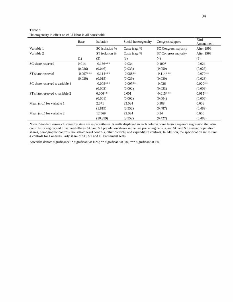
94

Table 8

Heterogeneity in effect on child labor in all households

Base Isolation Social heterogeneity Congress support 73rd

Amendment

Variable 1 SC isolation % Caste frag. % SC Congress majority After 1993

Variable 2 ST isolation % Caste frag. % ST Congress majority After 1993

(1) (2) (3) (4) (5)

SC share reserved 0.014 -0.166*** -0.034 0.100* -0.024

(0.026) (0.046) (0.033) (0.050) (0.026)

ST share reserved -0.097*** -0.114*** -0.088** -0.114*** -0.070**

(0.029) (0.015) (0.029) (0.030) (0.028)

SC share reserved x variable 1 -0.008*** -0.005** -0.026 0.020**

(0.002) (0.002) (0.023) (0.009)

ST share reserved x variable 2 0.006*** 0.001 -0.015*** 0.015**

(0.001) (0.002) (0.004) (0.006)

Mean (s.d.) for variable 1 2.071 93.024 0.388 0.606

(1.819) (3.552) (0.487) (0.489)

Mean (s.d.) for variable 2 12.569 93.024 0.24 0.606

(10.659) (3.552) (0.427) (0.489)

Notes: Standard errors clustered by state are in parentheses. Results displayed in each column come from a separate regression that also

controls for region and time fixed effects, SC and ST population shares in the last preceding census, and SC and ST current population

shares, demographic controls, household level controls, other controls, and expenditure controls. In addition, the specification in Column

4 controls for Congress Party share of SC, ST and all Parliament seats.

Asterisks denote significance: * significant at 10%; ** significant at 5%; *** significant at 1%

95

Table 9

Heterogeneity in effect on child labor in all households by gender

Panel A Total Boys Working

Base Isolation

Social

heterogeneity Congress support

73rd

Amendment

Variable 1 SC isolation % Caste frag. % SC Congress majority After 1993

Variable 2 ST isolation % Caste frag. % ST Congress majority After 1993

(1) (2) (3) (4) (5)

SC share reserved -0.006 -0.105*** -0.036* 0.032 -0.025*

(0.014) (0.026) (0.017) (0.028) (0.013)

ST share reserved -0.049*** -0.058*** -0.039** -0.056*** -0.034**

(0.015) (0.008) (0.015) (0.016) (0.707)

SC share reserved x variable 1 -0.005*** -0.003*** -0.016 0.012**

(0.001) (0.001) (0.013) (0.005)

ST share reserved x variable 2 0.003*** 0.001 -0.007** 0.008**

(0.001) (0.001) (0.003) (0.004)

Panel B Total Girls Working

Base Isolation

Social

heterogeneity Congress support

73rd

Amendment

Variable 1 SC isolation % Caste frag. % SC Congress majority After 1993

Variable 2 ST isolation % Caste frag. % ST Congress majority After 1993

(1) (2) (3) (4) (5)

SC share reserved 0.019 -0.061** 0.002 0.067** 0.001

(0.013) (0.021) (0.017) (0.024) (0.013)

ST share reserved -0.049*** -0.056*** -0.048*** -0.058*** -0.035**

(0.014) (0.008) (0.015) (0.014) (0.014)

SC share reserved x variable 1 -0.003** -0.002** -0.01 0.008*

(0.001) (0.001) (0.011) (0.004)

ST share reserved x variable 2 0.003*** 0.000 -0.008*** 0.007***

(0.001) (0.001) (0.002) (0.002)

Mean (s.d.) for variable 1 2.071 93.024 0.388 0.606

(1.819) (3.552) (0.487) (0.489)

Mean (s.d.) for variable 2 12.569 93.024 0.24 0.606

(10.659) (3.552) (0.427) (0.489)

Notes: Standard errors clustered by state are in parentheses. Results displayed in each column come from a separate regression

that also controls for region time fixed effects, SC and ST population shares in the last preceding census, and SC and ST current

population shares, demographic controls, household level controls, other controls, and expenditure controls. In addition, the

specification in Column 4 controls for Congress Party share of SC, ST and all Parliament seats.

Asterisks denote significance: * significant at 10%; ** significant at 5%; *** significant at 1%

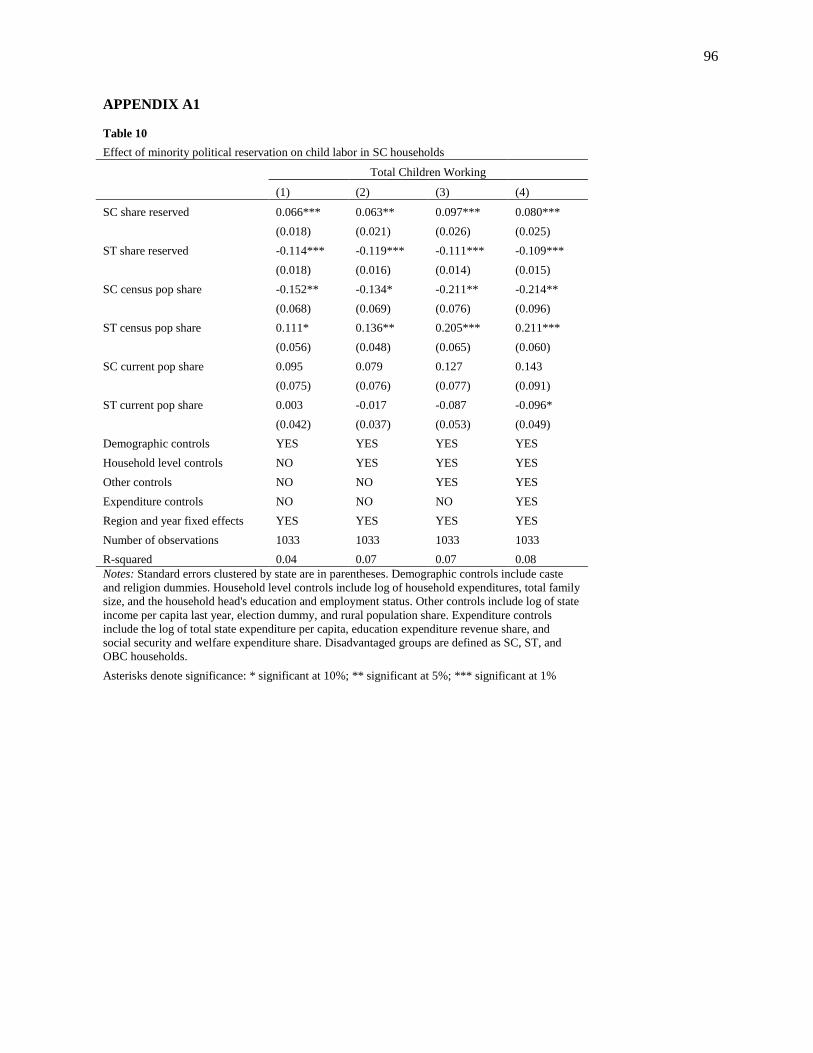
96

APPENDIX A1

Table 10

Effect of minority political reservation on child labor in SC households

Total Children Working

(1) (2) (3) (4)

SC share reserved 0.066*** 0.063** 0.097*** 0.080***

(0.018) (0.021) (0.026) (0.025)

ST share reserved -0.114*** -0.119*** -0.111*** -0.109***

(0.018) (0.016) (0.014) (0.015)

SC census pop share -0.152** -0.134* -0.211** -0.214**

(0.068) (0.069) (0.076) (0.096)

ST census pop share 0.111* 0.136** 0.205*** 0.211***

(0.056) (0.048) (0.065) (0.060)

SC current pop share 0.095 0.079 0.127 0.143

(0.075) (0.076) (0.077) (0.091)

ST current pop share 0.003 -0.017 -0.087 -0.096*

(0.042) (0.037) (0.053) (0.049)

Demographic controls YES YES YES YES

Household level controls NO YES YES YES

Other controls NO NO YES YES

Expenditure controls NO NO NO YES

Region and year fixed effects YES YES YES YES

Number of observations 1033 1033 1033 1033

R-squared 0.04 0.07 0.07 0.08

Notes: Standard errors clustered by state are in parentheses. Demographic controls include caste

and religion dummies. Household level controls include log of household expenditures, total family

size, and the household head's education and employment status. Other controls include log of state

income per capita last year, election dummy, and rural population share. Expenditure controls

include the log of total state expenditure per capita, education expenditure revenue share, and

social security and welfare expenditure share. Disadvantaged groups are defined as SC, ST, and

OBC households.

Asterisks denote significance: * significant at 10%; ** significant at 5%; *** significant at 1%

97

Table 11

Effect of minority political reservation on child labor in ST households

Total Children Working

(1) (2) (3) (4)

SC share reserved 0.027 0.006 0.108 0.053

(0.052) (0.047) (0.065) (0.077)

ST share reserved -0.007 0.006 0.040 0.055

(0.132) (0.126) (0.141) (0.146)

SC census pop share -0.188 -0.136 -0.202 0.096

(0.478) (0.443) (0.337) (0.476)

ST census pop share 0.146 0.129 0.228 0.295

(0.226) (0.210) (0.283) (0.206)

SC current pop share 0.126 0.091 0.068 -0.194

(0.515) (0.477) (0.374) (0.480)

ST current pop share -0.140 -0.138 -0.256 -0.350**

(0.126) (0.118) (0.179) (0.144)

Demographic controls YES YES YES YES

Household level controls NO YES YES YES

Other controls NO NO YES YES

Expenditure controls NO NO NO YES

Region and year fixed effects YES YES YES YES

Number of observations 544 544 544 544

R-squared 0.06 0.07 0.08 0.08

Notes: Standard errors clustered by state are in parentheses. Demographic controls include caste

and religion dummies. Household level controls include log of household expenditures, total family

size, and the household head's education and employment status. Other controls include log of state

income per capita last year, election dummy, and rural population share. Expenditure controls

include the log of total state expenditure per capita, education expenditure revenue share, and

social security and welfare expenditure share. Disadvantaged groups are defined as SC, ST, and

OBC households.

Asterisks denote significance: * significant at 10%; ** significant at 5%; *** significant at 1%

98

References

Alesina, A., Baqir, R. & Easterly, W. (1999). Public Goods and Ethnic Divisions. Quarterly Journal of

Economics, 114(4), pp.1243-1284.

Alcarez, C., Chiquiar, D., & Salcedo, A. (2012). Remittances, schooling, and child labor in Mexico. Journal

of Development Economics, 97, 156-165.

Amuedo-Dorantes, C. & Pozo, S. (2010). Accounting for Remittance and Migration Effects on Children's

Schooling. World Development, 38(12), 1747-1759.

Antman, F. (2011). International Migration and Gender Discrimination among Children Left Behind.

American Economic Review, 101(3), 645-649.

Antman, F. (2012a). International Migration, Household Decision-Making, and Gender Discrimination in

the Allocation of Household Resources. Department of Economics, University of Colorado at

Boulder.

Antman, F. (2012b). The Impact of Migration on Family Left Behind. IZA Discussion Paper, No. 6374..

Aslam, M., & Kingdon, G. G. (2008). Gender and household education expenditure in Pakistan. Applied

Economics, 40, 2573-2591.

Babu, S. (2006). Child Labour in India: Problems in Conceptualisation. Think India Quarterly, 9(3).

Bacolod, M., & Ranjan, P. (2008). Why Children Work, Attend School, or Stay Idle: The Roles of Ability

and Household Wealth. Economic Development and Cultural Change, 56, 791-828.

Banerjee, A. and Somanathan, R. (2007). The Political Economy of Public Goods: Some Evidence from

India. Journal of Development Economics, pp. 287-314.

Bardhan, P., Mookherjee, D., & Parra Torrado, M. L. (2010). The Impact of Political Reservation in West

Bengal Local Governments on Anti-Poverty Targeting. Journal of Globalization and Development,

1(1).

Basu, K., & Tzannatos, Z. (2003). The Global Child Labor Problem: What Do We Know and What Can

We Do? The World Bank Economic Review, 17(2), 147-173.

Basu, K., & Van, P. H. (1998, June). The Economics of Child Labor. The American Economic Review,

88(3), 412-427.

Becker, G. (1960). An Economic Analysis of Fertility. Demographic and Economic Change in Developed

Countries, 209-240.

Becker, G. (1974). A Theory of Social Interactions. Journal of Political Economy, 82(6), 1063-1093.

Behrman, J. (1997). Women's Schooling and Child Education: A Survey. Mimeo, University of

Pennsylvania.

99

Berry, J. (2013). Child Contol in Education Decisions: An Evaluation of Targeted Incentives to Learn in

India. Cornell University.

Bertrand, M., Hanna, R., & Mullainathan, S. (2010, February). Affirmative Action in Education: Evidence

from Engineering College Admissions in India. Journal of Public Economics, 94(1-2), 16-29.

Besley, T., Pande, R., Rahman, L., & Rao, V. (2004, April-May). The Politics of Public Good Provision:

Evidence from Indian Local Governments. Journal of the European Economic Association Papers

and Proceeedings, 2(2-3), 416-426.

Bhalotra, S., & Heady, C. (2003). Child Farm Labor: The Wealth Paradox. World Bank Economic Review,

17(2), 197-227.

Binder, M., & Scrogin, D. (1999, October). Labor Force Participation and Household Work of Urban

Schoolchildren in Mexico: Characteristics and Consequences. Economic Development and

Cultural Change, 48(1), 123-154.

Blanco Allasi, F. (2009). Assessing the gender gap: Evidence from SIMPOC surveys. International Labour

Organization, International Programme on the Elimination of Child Labour (IPEC), Statistical

Information and Monitoring Programme on Child Labour (SIMPOC).

Blunch, N.-H., & Verner, D. (2000, November). Revisiting the Link Between Poverty and Child Labor.

The World Bank Policy Research Working Paper 2488.

Blundell, R., Chiappori, P.-A., & Meghir, C. (2005, December). Collective Labor Supply with Children.

Journal of Political Economy, 113(6), 1277-1306.

Bobonis, G. (2009). Is the Allocation of Resources within the Household Efficient? New Evidence from a

Randomized Experiment. Journal of Political Economy, 117(3), 453-503.

Booth, A., & Tamura, Y. (2009). Impact of Paternal Temporary Absence on Children Left Behind. The

Australian National University, Centre for Economic Policy Research Discussion Paper No. 617.

Botezat, A. & Pfeiffer, F. (2014). The Impact of Parents Migration on the Well-being of Children Left

Behind: Initial Evidence from Romania. IZA Discussion Paper No. 8225.

Bourguignon, F., & Chiappori, P.-A. (1992). Collective models of household behavior. European Economic

Review, 36, 335-364.

Bourguignon, F., Browning, M., & Chiappori, P.-A. (2009). Efficient Intra-Household Allocation and the

Distribution Factors: Implications and Identification. The Review of Economic Studies, 76, 503-

528.

Boutin, D. (2014). Remittances and Child Labour in Africa: Evidence from Burkina Faso. IZA Discussion

Paper No. 8007.

Browning, M. (1992, September). Children and Household Economic Behavior. Journal of Economic

Literature, 30, 1434-1475.

100

Browning, M., Bourguignon, F., Chiappori, P.-A., & Lechene, V. (1994, December). Income and

Outcomes: A Structural Model of Intrahousehold Allocation. Journal of Political Economy, 102(6),

1067-1096.

Bureau of International Labor Affairs. (n.d.). Retrieved from United States Department of Labor:

http://www.dol.gov/ilab/media/reports/iclp/sweat/mexico.htm

Burton, P., Phipps, S., & Curtis, L. (2002, May). All in the Family: A Simultaneous Model of Parenting

Style and Child Conduct. Women, Children, and the Labor Market, 92(2).

Case, A., & Deaton, A. (2003). Consumption, Health, Gender, and Poverty. The World Bank Policy

Research Working Paper No. 3020.

Chattopadhyay, R., & Duflo, E. (2004, September). Women as Policy Makers: Evidence from a

Randomized Policy Experiment in India. Econometrica, 72(5), 1409-1443.

Chiappori, P.-A. (1988). Nash-bargained Household Decisions: A Comment. International Economic

Review, 29, 791-796.

Chiappori, P.-A. (1992). Collective Labor Supply and Welfare. Journal of Political Economy, 100(3), 437-

467.

Childline India Foundation. (2013). Child Protection & Child Rights. Retrieved from

http://www.childlineindia.org.in/child-labour-india.htm

Chin, A., & Prakash, N. (2011). The redistributive effects of political reservation for minorities: Evidence

from India. Journal of Development Economics, 96, 265-277.

Chiuri, M. C. (2000). Individual decisions and houshold demand for consumption and leisure. Research in

Economics, 54, 277-324.

Comola, M. & Mendola, M. (2014). The Formation of Migrant Networks. IZA Discussion Paper No. 7981.

Dauphin, A., El Lahga, A.-R., Fortin, B., & Lacroix, G. (2011, June). Are Children Decision-Makers Within

the Household. The Economic Journal, 121, 871-903.

De Paoli, A., & Mendola, M. (2012). Does International Migration Increase Child Labor? University of

Milan, Department of Economics, Management and Statistics Working Paper No. 231.

Deaton, A. (1987). The Allocation of Goods within the Household: Adults, Children, and Gender. LSMS

Working Paper No. 39.

Deaton, A. (1989). Looking for Boy-Girl Discrimination in Household Expenditure Data. The World Bank

Economic Review, 3(1), 1-15.

Deaton, A. (1997). The Analysis of Household Surveys: A Microeconomic Approach to Development

Policy. Baltimore and London: The World Bank and The Johns Hopkins University Press.

101

Dehejia, R., & Gatti, R. (2005, July). Child Labor: The Role of Financial Development and Income

Variability Across Countrie. Economic Development and Cultural Change, 53(4), 913-932.

Deolalikar, A. (1997, January). The Determinants of Primary School Enrollment and Household Schooling

Expenditures in Kenya: Do They Vary by Income? University of Washington, Department of

Economics.

Diallo, Y., Hagemann, F., Etienne, A., Gurbuzer, Y., & Mehran, F. (2010). Global child labour

developments: Measuring trends from 2004 to 2008. International Labour Organization. Statisitcal

Information and Monitoring Programme on Child Labour (SIMPOC) for the International

Programme on the Elimination of Child Labour (IPEC).

Doepke, M., & Krueger, D. (2006). Origins and Consequences of Child Labor Restrictions: A

Macroeconomic Perspective. NBER Working PaperNo. 12665.

Doepke, M., & Zilibotti, F. (2009, June). Do International Labor Standards Contribute to the Persistence of

the Child Labor Problem. NBER Working Paper 15050.

Duflo, E. (2005, April-May). Why Political Reservations? Journal of the European Economic Association,

3(2-3), 668-678.

Duflo, E., & Udry, C. (2004). Intrahousehold Resource Allocation in Cote D'Ivoire: Social Norms, Separate

Accounts and Consumption Choices. NBER Working Paper No. w10498.

Duflo, E., Fischer, G., & Chattopadhyay, R. (2008, July). Efficiency and Rent Seeking in Local

Government: Evidence from a Randomized Policy Experiment in India. MIT Working Paper.

Edmonds, E. (2005, Winter). Does Child Labor Decline with Improving Economic Status? Journal of

Human Resources, 40(1), 77-99.

Edmonds, E. (2006, Winter). Child labor and schooling responses to anticipated income in South Africa.

Journal of Development Economics, 40(1), 386-414.

Edmonds, E. (2008). Child Labor. Handbook of Development Economics.

Edmonds, E. (2009). Defining chid labour: A review of the definitions of child labour in policy research.

ILO International Programme on the Elimination of Child Labour.

Edmonds, E., Pavcnik, N. & Topalova, P. (2010). Trade Adjustment and Human Capital Investments:

Evidence form Indian Tariff Reform. American Economic Journal, 2(4), pp. 42-75.

Edmonds, E., & Turk, C. (2002). Child Labor in Transition in Vietnam. World Bank, Macroeconomic and

Growth, Development Research Group Policy Paper 2774.

Emerson, P. M., & Souza, A. P. (2003, January). Is There a Child Labor Trap: Intergenerational Persistence

of Child Labor in Brazil. Economic Development and Cultural Change, 51(2), 375-398.

Farfan, G., Genoni, M., Rubalcava, L., Terul, G., & Thomas, D. (2011). Oportunidades and its Impact on

Child Nutrition. Working Paper.

102

Fortin, B., & Lacroix, G. (1997, July). A Test of the Unitary and Collective Models of Household Labour

Supply. The Economic Journal, 107(443), 933-955.

Frankenberg, E. and L. Karoly. (1995, November). "The 1993 Indonesian Family Life Survey: Overview

and Field Report." RAND, Santa Monica, CA.

Frankenberg, E. and D. Thomas. (2000, March) "The Indonesia Family Life Survey (IFLS): Study Design

and Results from Waves 1 and 2". RAND, Santa Monica, CA. DRU-2238/1-NIA/NICHD.

Galanter, M. (1984). Competing Equalities: Law and the Backward Classes in India. Berkeley: University

of California Press.

Giannelli, G.C. & Mangiavacchi, L. (2014). Children's Schooling and Parental Migration: Empirical

Evidence on the "Left Behind" Generation in Albania. IZA Discussion Paper No. 4888.

Gibson, J., McKenzie, D. Stillman, S. (2009, May). The Impacts of International Migration on Remaining

Household Members: Omnibus Results from a Migration Lottery Program. CReAM Discussion

Paper No 20/09.

Gong, X., Soest, A. v., & Zhang, P. (2000). Sexual Bias and Household Consumption: A Semiparametric

Analysis of Engel Curves in Rural China. IZA Discussion Paper No. 212.

Government of India, Minsitry of Home Affairs. (2011). Census 2011. Retrieved from

http://censusindia.gov.in/2011-common/censusdataonline.html

Government of India, Ministry of Labour & Employment. (2013). Child Labour Acts, Rules and Schedule.

Retrieved from http://labour.nic.in/content/division/acts-and-rules.php

Government of India, Planning Commission, (2012, March). Press Note on Poverty Estimates, 2009-10.

Retrieved from http://planningcommission.nic.in/news/press_pov1903.pdf

Grogger, J., & Ronan, N. (1995). The Intergenerational Effects of Fatherlessness on Educational Attainment

and Entry-Level Wages. National Longitudianl Survey Discussion Paper No. 96-30, Bureau of

Labor Statistics.

Grootaert, C., & Kanbur, R. (1995). Child labour: An economic perspective. International Labour Review,

134(2).

Harbaugh, W., Krause, K., & Berry, T. (2001, December). GARP for Kids: On the Development of Rational

Choice Behavior. The American Economic Review, 91(5).

Harbaugh, W., Krause, K., & Liday, S. G. (2003). Bargaining By Children.

Haveman, R., & Wolfe, B. (1995). The Determinants of Children's Attainments: A Review of Methods and

Findings. Journal of Economic Literature, 33, 1829-1878.

Hildebrandt, N. & McKenzie, D. (2005, April). The Effects of Migration on Child Health in Mexico. World

Bank Policy Research Working Paper 3573.

103

Hoddinott, J., & Haddad, L. (1995). Does Female Income Share Influence Household Expenditures?

Evidence from Cots D'Ivoire. Oxford Bulletin of Economics and Statistics, 57(1), 77-96.

International Labour Organization. (2014). Labour migration in Indonesia:

http://www.ilo.org/jakarta/areasofwork/labour-migration/lang--en/index.htm

International Labour Organization. (2011). Retrieved April 18, 2011, from ILO Conventions and

Recommendations on Child Labour: http://www.ilo.org/ipec/Action/Time-

BoundProgrammes/Legal/Conventions/lang--en/index.htm

International Labour Organization. (2013). What is child labour? Retrieved from International Programme

on the Elimination of Child Labour (IPEC): http://www.ilo.org/ipec/facts/lang--en/index.htm

International Organization for Migration. (2013). Indonesia.

https://www.iom.int/cms/en/sites/iom/home/where-we-work/asia-and-the-pacific/indonesia.html

Irving, M., & Kingdon, G. G. (2008). Gender patterns in household health expenditure allocation: A study

of South Africa. CSAE WPS/2008-32.

Iverson, V. (2002). Autonomy in Child Labor Migrants. World Development, 30, 817-834.

Jafarey, S., & Lahiri, S. (2002). Will trade sanctions reduce child labour? The role of credit markets. Journal

of Development Economics, 68, 137-156.

Kalwij, A., & Salverda, W. (2007). The Effects of Changes in Household Demographics and Employment

on Consumer Demand Patterns. Applied Economics, 39, 1447-14460.

Kantor, P. (2003). Women's Empowerment Through Home-based Work: Evidence from India.

Development and Change, 34(3), 425-445.

Krishnan, N. (2007). Political Reservation and Rural Public Good Provision in India. Boston University.

Krueger, A. B. (1996, June). Observations on International Labor Standards and Trade. NBER Working

Paper 5632.

Kumar, A. (2013). Preference based vs. market based discrimination: Implications for gender differentials

in child labor and schooling. Journal of Development Economics, 105, 64-68.

Lancaster, G., Maitra, P., & Ray, R. (2008). Household Expenditure Patterns and Gender Bias: Evidence

from Selected Indian States. Oxford Development Studies, 36(2), 133-157.

Leser, C. E. (1963). Forms of Engel Functions. Econometrica, 31(4), 694-703.

Levison, D., & Moe, K. (1998, Spring). Household Work as a Deterrent to Schooling: An Analysis of

Adolescent Girls in Peru. The Journal of Developing Areas, 32(3), 339-356.

Levison, D., Anker, R., Ashraf, S., & Barge, S. (1996). Is Child Labor Really Necessary in India's Carpet

Industry? Employment Department, International Labour Office, Labour Market Papers 15.

104

Levison, D., Moe, K., & Knaul, F. (2001). Youth Education and Work in Mexico. World Development,

29(1), 167-188.

Levison, D., Moe, K., & Knaul, F. (2008). Marking Time: An Analysis of Youth Hours of Work and Study

in Urban Mexico. Review of Development Economics, 12(4), 751-763.

Lundberg, S., & Pollack, R. (1993). Separate Spheres Bargaining and the Marriage Market. The Journal of

Political Economy, 101(6), 988-1010.

Lundberg, S., Romich, J., & Tsang, K. P. (2009). Decision-making by children. Review of Economics of

the Household, 7, 1-30.

Maitra, P., & Ray, R. (2002). Household resources, expenditure patterns and resource pooling: evidence

from South Africa. Mimeo: University of Tasmania.

Manser, M., & Brown, M. (1980, February). Marriage and Household Decision-Making: A Bargaining

Analysis. International Economic Review, 21(1), 31-44.

McElroy, M. B., & Horney, M. J. (1981, June). Nash-Bargained Household Decisions: Toward a

Generalization of the Theory of Demand. International Economic Review, 22(2), 333-349.

Moehling, C. (2005). She has suddenly become powerful: youth employment and household decision

making in the early twentieth century. Journal of Economic History, 65, 414-438.

Moehling, C. (2006). Children's pay envelopes and the family purse: the impact of children's income on

household expenditures. Rutgers University.

Mookherjee, D. (2012, October). Accountability of Local and State Governments in India: An Overview

of Recent Research. Boston University.

Muralidharan, K. (2007, September). Public Service In India: Challenges and Opportunities. (University

of Pennsylvania, Center for the Advanced Study of India) Retrieved from

http://casi.sas.upenn.edu/iit/muralidharan

Nguyen, T., & Purnamasari, R. (2011). Impacts of International Migration and Remittances on Child

Outcomes and Labor Supply in Indonesia. The World Bank Policy Research Working Paper No.

5591.

Office of the United Nations High Commissioner for Human Rights. (1989). Retrieved from Convention of

the Rights of the Child: http://www2.ohchr.org/english/law/crc.htm

Ozler, B., Datt, G., & Ravallion, M. (1996). A Database on Poverty and Growth in India. World Bank

Rsearch Group, Washington DC.

Pande, R. (2003, September). Can Mandated Political Representation Increase Policy Influence for

Disadvantaged Minorities? Theory and Evidence from India. The American Economic Review,

93(4), 1132-1151.

105

Randazzo, T. & Piracha, M. (2014). Remittances and Household Expenditure Behaviour in Senegal. IZA

Discussion Paper No. 8106.

Reggio, I. (2011). The Influence of the Mother's Power on Her Child's Labor in Mexico. Journal of

Development Economics, 96, 95-105.

Reserve Bank of India, India's Central Bank. (2002). State Finances: A Study of Budgets 2011-2002.

Rubalcava, L., & Teruel, G. (2006). User's Guide for the Mexican Family Life Survey First Wave.

Rubalcava, L., & Teruel, G. (2008). User's Guide for the Mexican Family Life Survey Second Wave.

Ruiz, A. M., & Vazquez, R. M. (2013). Nina o Nino? Un estudio sobre las preferencias de los padres

Mexicanos por el sexo sus hijos. Estudios Economicos, 28(2), 217-248.

Strauss, J., K. Beegle, B. Sikoki, A. Dwiyanto, Y. Herawati and F. Witoelar. "The Third Wave of the

Indonesia Family Life Survey (IFLS): Overview and Field Report", March 2004. WR-144/1

NIA/NICHD.

Strauss, J., F. Witoelar, B. Sikoki and A.M. Wattie. "The Fourth Wave of the Indonesian Family Life

Survey (IFLS4): Overview and Field Report". April 2009. WR-675/1-NIA/NICHD.

Strulik, H. (2004, July). Child Mortality, Child Labour and Economic Development. The Economic

Journal, 114(497), 547-568.

Strulik, H. (2008, January). The Role of Poverty and Community Norms in Child Labor and Schooling

Decisions. University of Hannover, Department of Economics.

Tauson, M. (2009). Child Labor in Latin America: Poverty as Cause and Effect. Human Rights & Human

Welfare.

The World Bank Group. (2013a, January 18). Children at Work in Mexico, Still a Major Issue. Retrieved

from http://www.worldbank.org/en/news/feature/2013/01/18/children-at-work-in-mexico-still-a-

major-issue

The World Bank Group. (2013b). World Development Indicators. Retrieved from

http://www.worldbank.org/

Udry, C. (1996). Gender, Agriculatural Production, and the Theory of the Household. Journal of Political

Economy, 104(5), 1010-1046.

UNICEF. (2011). The Situation of Children in India: A Profile.

Vermeulen, F. (2002). Collective Household Models: Principles and Main Results. Journal of Economic

Surveys, 16(4).

Vermeulen, F. (2005). And the Winner Is... An Empirical Evaluation of Unitary and Collective Labour

Supply Models. Empirical Economics, 30, 711-734.

106

Viljoen, L. (1998). Factors that influence household and individual clothing expenditure: A review of

research and related literature. Journal of Family Ecology and Consumer Sciences, 26(1).

Wahba, J. (2005). The Influence of Market Wages and Parental History on Child Labor and Schooling in

Egypt. IZA Discussion Paper No. 1771.

Working, H. (1943). Statistical Laws of Family Expenditure. Journal of the American Statistical

Association, 38(221), 43-56.

Yang, D. (2008). International Migration, Remittances and Household Investment: Evidence from

Philippine Migrants' Exchange Rate Shocks. The Economic Journal, 118, 591-630.

Zimmerman, L. (2011). Reconsidering Gender Bias in Intra-Household Allocation in India. IZA Discussion

Paper No. 5687.