essays on asset pricing in open economies · essays on asset pricing in open economies ......
TRANSCRIPT

Essays on Asset Pricing in Open Economies
Andreas Stathopoulos
Submitted in partial fulfillment of the
requirements for the degree
of Doctor of Philosophy
under the Executive Committee
of the Graduate School of Arts and Sciences
COLUMBIA UNIVERSITY
2010

UMI Number: 3420802
All rights reserved
INFORMATION TO ALL USERS The quality of this reproduction is dependent upon the quality of the copy submitted.
In the unlikely event that the author did not send a complete manuscript and there are missing pages, these will be noted. Also, if material had to be removed,
a note will indicate the deletion.
TJMT Dissertation Publishing
UMI 3420802 Copyright 2010 by ProQuest LLC.
All rights reserved. This edition of the work is protected against unauthorized copying under Title 17, United States Code.
ProQuest LLC 789 East Eisenhower Parkway
P.O. Box 1346 Ann Arbor, Ml 48106-1346

A B S T R A C T
Essays on Asset Pricing in Open Economies
Andreas Stathopoulos
Chapter 1 proposes a two-country general equilibrium model with external habits and
home-biased preferences that addresses a number of international finance puzzles. Specifi
cally, the model reconciles the high degree of international risk sharing implied by relatively
smooth exchange rates with the modest cross-country consumption growth correlations seen
in the data, resolving the Brandt, Cochrane and Santa-Clara (2006) puzzle. Furthermore,
the model matches the empirically observed low correlation between exchange rate changes
and international consumption growth rate differentials. For both effects, the fundamental
mechanism is time variation in consumption growth volatility, which is endogenously gen
erated through international trade. Asset prices depend on a weighted average of the two
countries' time-varying risk aversion, with the weights determined by the wealth and degree
of home bias of each country. Simulation results indicate that the model is successful in
matching key empirical asset pricing, exchange rate and international trade moments.
Chapter 2 examines international portfolio choice in a two-country general equilib
rium setting which features time-varying risk aversion generated by external habit forma
tion. I show that, under complete markets, home bias in the consumption preferences leads
to significant portfolio home bias due to differential hedging demands. Domestic (foreign)
agents shift their portfolio towards domestic (foreign) assets, so as to better hedge against
adverse changes in their conditional risk aversion. Furthemore, the model generates realistic
asset pricing moments, thus reconciling international portfolio choice with asset pricing.

Contents
List of Tables iv
List of Figures v
Acknowledgments vi
Chapter 1 Asset Prices and Risk Sharing in Open Economies 1
1.1 Introduction 1
1.2 The model 7
1.2.1 The structure of the economy 7
1.2.2 Preferences 8
1.2.3 Prices and exchange rates 10
1.3 Equilibrium prices and quantities 11
1.3.1 The planner's problem 11
1.3.2 Consumption 12
1.3.3 International risk sharing 15
1.3.4 International trade and the real exchange rate 18
1.3.5 Wealth and welfare weights 20
1.4 Asset prices 21
1.4.1 Risk-free rates 22
1.4.2 Total wealth portfolio prices 23
1.4.3 Total wealth portfolio excess returns 25
1.4.4 Asset prices and exchange rates 27
1.5 Simulation 27
1.5.1 Definitions and data 27
i
1.5.2 The endowment processes 29
1.5.3 Parameter calibration 30
1.5.4 Simulation results 31
1.6 Conclusion 37
1.7 Appendix 38
1.7.1 Solution to the planner's problem 38
1.7.2 Pricing kernels 39
1.7.3 Endowment parameter calibration 41
1.7.4 Empirical examination of endowment cointegration 42
1.7.5 Proofs 43
Chapter 2 Portfolio Choice in Open Economies wi th External Habit For
mat ion 57
2.1 Introduction 57
2.2 The economic setting 65
2.2.1 Endowments 65
2.2.2 Assets 66
2.2.3 Preferences 66
2.2.4 Prices and exchange rates 67
2.2.5 The agents' problem 68
2.3 Equilibrium 69
2.3.1 The planner's problem formulation 71
2.3.2 Quantities and prices 74
2.3.3 Consumption volatility and risk sharing 77
2.4 The portfolio autarky case 78
2.5 The complete markets case 81
2.5.1 Equilibrium portfolios 82
2.5.2 Home bias 87
2.5.3 Simulation results 88
2.6 Conclusion 90
2.7 Appendix 91
2.7.1 Competitive equilibrium 91
ii

2.7.2 The planner's problem solution 93
2.7.3 Proofs 94
in

List of Tables
1.1 Endowment calibration 48
1.2 Calibration parameters 49
1.3 Simulation results: endowment and consumption 50
1.4 Simulation results: international trade and the real exchange rate 51
1.5 Simulation results: asset prices and returns 52
1.6 Calibration parameters: no endowment cointegration 53
1.7 Johansen cointegration tests 54
2.1 Moments: portfolio autarky case 98
2.2 Quantities and prices: complete markets case 99
2.3 Portfolios: complete markets case 100
iv

List of Figures
1.1 Empirical probability density functions of surplus consumption ratios . . . . 55
1.2 Simulated moments for different values of a 56
v

Acknowledgments
I am deeply indebted to Geert Bekaert and Tano Santos, my advisors at Columbia Business
School, for their guidance, encouragement and great support throughout my PhD studies.
I am also grateful to the rest of my dissertation committee, Pierre Collin-Dufresne, Emi
Nakamura and Jon Steinsson for their invaluable advice. Finally, I thank Michael Adler,
Andrew Ang, Patrick Bolton, Charles Calomiris, John Cochrane, John Donaldson, Robert
Hodrick, Gur Huberman, Michael Johannes, Martin Lettau, Lars Lochstoer, Tomasz Pisko-
rski, Veronica Rappoport, Paolo Siconolfi, Suresh Sundaresan, Maxim Ulrich, Neng Wang
and seminar participants at the Bank of Canada, Columbia University, Emory Univer
sity, Georgetown University, the Federal Reserve Board, Imperial College, London Business
School, the London School of Economics, McGill University, MIT, NYU, the University of
Piraeus, the University of Southern California, the University of Texas - Austin and the
University of Wisconsin - Madison for helpful comments.
VI

To my parents
vn

Chapter 1
Asset Prices and Risk Sharing in
Open Economies
1.1 Introduction
This Chapter presents a model which highlights, in a tractable way, the links between asset
prices, exchange rates and international risk sharing generated by international trade in
goods and assets. The model proposes a solution to a number of international finance puzzles
that are related to the connection between the aforementioned three economic concepts,
with the primary focus being on the international risk sharing puzzle. Furthermore, the
model clearly illustrates how international trade affects equity prices and risk-free rates vis
a-vis the closed economy benchmark and explicitly connects real exchange rates and equity
prices.
The international risk sharing puzzle, illustrated in detail in Brandt, Cochrane and
Santa-Clara (2006), is the apparent disconnect between relatively modest empirical cross
country consumption growth rate correlations and the extremely high degree of international
risk sharing implied by the relatively low real exchange rate volatility observed in the data.1
If financial markets are complete, the key relationship that generates the links between asset
and currency prices and risk sharing is the no-arbitrage relationship
^±1 = ^±1 (1.1) Mt+r Et V '
'As will be discussed later, real exchange rate volatility is low only compared to asset return volatility; it is quite high compared to macroeconomic (income or consumption) volatility.

2
where Mt+\ and Mt*+1 are the home and foreign stochastic discount factor (SDF), respec
tively, and Et is the real exchange rate (domestic price of foreign currency, in real terms, i.e.
an increase in Et denotes a real depreciation of the domestic currency). This relationship
is not without assumptions: it holds only when financial markets are frictionless, in the
sense that investors in each country can freely invest in assets denominated in any of the
two currencies.2 Perfect risk sharing between the two countries means Mf*+1 = Mt+i, which
implies a constant real exchange rate.3
Taking logs and then unconditional variances on each side of (1.1), we get
var{m*t+l) + var(mt+1) - 2a(mt+1)a(m*t+1)p(mt+1,m^+1) = var{Aet+1)
with small letters denoting the log of their capital letter counterpart. Using the logic of
Hansen and Jagannathan (1991) volatility bounds, the high Sharpe ratios we observe in
asset markets imply very high pricing kernel volatility. Unless the correlation between the
two pricing kernels is extremely high, high kernel volatility cannot be reconciled with the
empirically observed modest levels of real exchange rate volatility. Setting, for example,
a{mt+{) — a(m^+1) = 50% and considering a(Aet+i) = 10% (in line with empirical real
exchange rate volatility for major currency pairs), we can easily see that prices imply that
p(mt+i,mt+1) = 0.98. Under CRRA preferences, mt+\ = log(3 — 7 A c t + i and rrc£+1 =
log fi — jACf+1, so p(mt+\, m^+1) = p(Act + i , Ac£+1). Then, to square prices with quantities,
we need p(Act+i, Acj+ 1) = 0.98; unfortunately, the observed cross-country consumption
growth correlations are typically much lower, with correlations of 0.9 and above not being
even remotely plausible. The only way we can have e.g. p{mt+\,m*j.+1) — 0.3 (in line
with empirical cross-country consumption growth correlations) is if a(Aet+i) = 65%; as
mentioned above, this is highly counterfactual. This, in a nutshell, is the puzzle: prices tell
2Complete markets are not necessary for (1.1) to hold. In the presence of market incompleteness, (1.1) holds with Mt+i being the (unique) projection of all (i.e. domestic and foreign) investors' intertemporal marginal rate of substi tution (IMRS), expressed in domestic currency units, on Xt+i, and M* + 1 the (unique) projection of all investors' IMRS, expressed in foreign currency units, on Xf+i, where Xt+i (X£+i) is the space spanned by the domestic (foreign) currency returns of all assets, domestic and foreign. See Backus, Foresi and Telmer (2001) and Brandt , Cochrane and Santa-Clara (2006).
3 In the international macroeconomics and finance literature, optimal risk sharing is sometimes defined as being equivalent to the achievement of a Pare to optimal allocation. In tha t case, (1) is the optimal risk sharing condition; for special cases of this condition, see, for example, Cole and Obstfeld (1991), Backus and Smith (1993), Lewis (1996) and Obstfeld and Rogoff (2000). This paper, following Brandt et el. (2006), uses the term "perfect risk sharing" to refer to the more stringent condition Mt+i = Mf*+1; the reason is tha t , as explained in detail in Brandt et al. (2006) and in this paper, the international risk sharing puzzle regards SDF correlations, not Pareto optimality.

3
us that risk is nearly perfectly shared among countries, but quantities tell us otherwise.
Consequently, any model that aims to explain the relationship between asset returns and
exchange rates should address international risk sharing, reconciling high unconditional
pricing kernel correlations with relatively modest unconditional consumption growth rate
correlations.
A related puzzle to be addressed is the exchange rate disconnect puzzle, illustrated
by Backus and Smith (1993). Starting with (1.1), it is easy to see that for CRRA preferences
we get
corr(Act+1 - Ac*t+1, Aet+1) = 1 (1.2)
irrespective of the value of 7. Backus and Smith (1993) derive this result in a more general
setting. However, in the data, consumption growth rate differentials appear to be decoupled
from real exchange rate changes; using data from 8 OECD countries, Backus and Smith
(1993) show that the average correlation between per capita consumption growth rate dif
ferentials and real exchange rate changes is -0.056, with a range of [-0.63, 0.21], a far cry
from the theoretical value of 1.
Another issue in international macroeconomics is the "remarkable", in the words of
Obstfeld and Rogoff (2000), volatility of real exchange rates. As mentioned earlier, from
the perspective of asset pricing, real exchange rate volatility is relatively small: asset return
volatility is around 15% — 20% per year, while pricing kernel volatility is even higher, of
the order of 50%. However, from the perspective of international macroeconomics, the
volatility of real exchange rate changes should not be far from consumption or income
growth volatility, around 1% — 3% per year; it is, instead, almost an order of magnitude
higher.
This Chapter proposes a two-country endowment model that incorporates external
habits and consumption home bias in preferences. In the model, the global economy is
comprised of two countries, each represented by a stand-in agent endowed with a stream of
a differentiated perishable good. Each of the two agents has Menzly, Santos and Veronesi
(2004) external habit preferences, with the habit defined on a home-biased, CES aggregated
consumption basket of the two goods. This model leads to an economically intuitive solution
4 Brandt et al. (2006) measure risk sharing using a risk sharing index, which also detects differences in scale. Since perfect risk sharing is the equalization of the two countries' pricing kernels, mt+i = 2mt+1 does not imply perfect risk sharing, although p{mt+i,ml+x) = 1. Therefore, high correlation is not sufficient for high risk sharing; it is, however, necessary.

4
to both the international risk sharing puzzle and the exchange rate disconnect puzzle.
Regarding the international risk sharing puzzle, the model implies that countries
indeed share risk to a very large degree through trade in goods and assets. Specifically, trade
generates endogenous time variation in consumption growth volatility: the conditionally
relatively less risk averse country assumes more of the global endowment risk. In other
words, the conditionally more risk averse country has low consumption risk, while the less
risk averse country has high consumption risk. On the other hand, the conditionally less risk
averse country has low conditional sensitivity to consumption growth risk, while the more
risk averse country is very sensitive to consumption risk. To understand how this resolves
the puzzle, consider the market price of consumption risk. Since, for each country, the
conditional market price of consumption risk is an increasing function of both conditional
risk aversion and conditional consumption growth volatility, the two effects (volatility and
sensitivity) push the relative market price of risk of the two countries to different directions.
However, since the magnitude of the two effects is almost equal, those two effects, combined,
balance each other, leading to a very high cross-country correlation of market prices of
risk and, thus, pricing kernels. However, cross-country consumption growth correlation is
modest, since there is no sensitivity effect to counter the volatility effect.
Regarding the exchange rate disconnect puzzle, habits decouple marginal utility
growth from consumption growth. This effect generates very low correlation between con
sumption growth rate differentials and real exchange rate changes, despite the fact that
the correlation between pricing kernel differentials and real exchange rate changes is, by
construction, perfect.
The model also sheds light on the issue of asset pricing in open economies. Specifi
cally, the model generates an economically intuitive solution for the price of the two coun
tries' total wealth portfolios: the price-dividend ratio of each total wealth portfolio is de
termined by a weighted average of the two countries' time-varying relative risk aversion
coefficients, with the weights depending on the initial wealth and the degree of home bias of
the two countries. When the economy is closed, the solution collapses to the Menzly, Santos
and Veronesi (2004) pricing results, so the model clearly illustrates how international trade
affects asset prices and returns. The connection of asset prices with exchange rates is also
straightforward: the real exchange rate is a function of both the endowment ratio and the
price-dividend ratios of the two total wealth portfolios. Thus, real exchange rate volatility

5
is generated by two economic mechanisms: time variation in relative endowments and time
variation in price-dividend ratios. The latter, asset pricing-related, mechanism amplifies
the effects of the former, endowment-related, mechanism, so real exchange rate changes are
much more volatile than endowment growth rates. The failure of most standard interna
tional macroeconomic models to generate substantial real exchange rate volatility can, thus,
be traced to their inability to generate time-varying asset price-dividend ratios.
This Chapter is part of the recent literature that focuses on the connections between
asset prices and exchange rates. The model in this Chapter builds on Pavlova and Rigobon
(2007). They use a Lucas (1982) two-country, two-good model to examine the effects of
the terms of trade on asset prices and exchange rates when preferences are characterized
by demand shocks. Inter aha, they use financial data to extract latent factors implied by
their model and show that those factors can be used to predict macroeconomic variables
and ameliorate puzzles arising in the international real business cycle literature. Despite its
success in addressing macroeconomic questions, the ability of their model to match asset
prices and returns is limited by its inability to generate time-varying asset price-dividend
ratios.5 Other international asset pricing models that focus on terms of trade effects are
Cole and Obstfeld (1991), Zapatero (1995) and Serrat (2001).
Recent papers extend standard asset pricing models to examine international finance
issues. Regarding habits, Verdelhan (2008a) uses a two-country, one-good model in which
each country has an exogenously specified i.i.d. consumption growth process and Campbell
and Cochrane (1999) external habit preferences. The model is able to explain the forward
premium puzzle, but generates real exchange rates that are both highly volatile, implying
poor international risk sharing, and excessively linked to consumption growth. Verdelhan
(2008b), a companion paper, assumes i.i.d. endowment growth and allows for international
trade characterized by proportional and quadratic trade costs, thus endogenizing consump
tion; the ability to share risk by international trade lowers real exchange rate volatility
to realistic levels, but the real exchange rate remains very closely linked to consumption
growth, so the Backus and Smith (1993) puzzle cannot be resolved.6 Bekaert (1996) ex-
5 To be precise, price-dividend ratios are non-stochastic. Specifically, when the time horizon is finite, the price-dividend ratio of each country's total wealth portfolio is a deterministic function of time. When the time horizon is infinite, the price-dividend ratio is constant.
6 The author suggests that this result may be caused by the one-good assumption. It should be noted that Verdelhan (2008b) does not examine international consumption growth correlations, so the paper does not explore the international risk sharing puzzle.

6
amines currency risk premia using a two-country monetary model which features durability
and habit persistence. Moore and Roche (2006) embed Campbell and Cochrane (1999)
preferences with "deep" habits (Ravn, Schmitt-Grohe and Uribe (2006)) in a flexible-price
monetary model in order to address both the exchange rate disconnect puzzle and the for
ward premium puzzle. Shore and White (2006) address the portfolio home bias puzzle with
a model that incorporates external habit formation. Aydemir (2008) uses a two-country,
one-good external habits model in order to examine international equity market return
correlations.
Colacito and Croce (2008a) utilize the Bansal and Yaron (2004) long-run risks frame
work in order to address the international risk sharing puzzle. They consider a two-country,
two-good closed economy endowment model in which each country has Epstein and Zin
(1989) preferences and an exogenously specified consumption growth process featuring a
slow moving, predictable component. They show that the puzzle can be resolved if the
two predictable components, the domestic and the foreign one, are highly correlated. In
Colacito and Croce (2008b), they extend their model to open economies, allowing for in
ternational trade and endogenizing consumption, in order to revisit the Cole and Obstfeld
(1991) results; they show that international portfolio diversification may produce significant
welfare gains in the presence of long-run risk.7 Bansal and Shaliastovich (2007) also use a
long-run risks model in order to, inter aha, address the forward premium puzzle.
Farhi and Gabaix (2008) propose a two-country rare disasters model to explain the
cross-country joint dynamics of exchange rates, bonds, stocks and options. Lustig and
Verdelhan (2006) use the Yogo (2006) model in order to empirically illustrate the effects of
consumption growth risk on currency risk premia.
One of the key assumptions of this Chapter is external habit formation. Habits,
internal or external, have been used in much of the recent asset pricing literature.8 The
present work postulates Menzly et al. (2004) external habits, which share the motivation
of Campbell and Cochrane (1999) habits, but model the inverse surplus consumption ratio.
Buraschi and Jiltsov (2007) use the same mean-reverting process for the inverse surplus
7As in Colacito and Croce (2007), matching the empirical volatility level of real exchange rate changes requires that long-run endowment shocks be highly internationally correlated.
8See, for example, Sundaresan (1989), Abel (1990), Constantinides (1990), Detemple and Zapatero (1991), Ferson and Constantinides (1991), Heaton (1995), Jermann (1998), Boldrin, Christiano and Fisher (2001) and Chan and Kogan (2002).

7
consumption ratio in order to study the term structure of interest rates.9
The rest of the Chapter is organized as follows. Section 2 describes the model. Sec
tion 3 presents the equilibrium macroeconomic prices and quantities and explains how the
international risk sharing puzzle is resolved. Section 4 explores the asset pricing implications
of the model. Section 5 reports the simulation results. Section 6 concludes. The Appendix
contains the proofs and all supplementary material not included in the main body of this
Chapter.
1.2 The model
1.2.1 T h e s t r u c t u r e o f t h e e c o n o m y
The world economy is comprised of two countries, Domestic and Foreign, each of which is
populated by a single risk-averse representative agent who receives an endowment stream
of a single differentiated perishable good: the domestic agent is endowed with the domestic
good, while the foreign agent is endowed with the foreign good. Economic activity takes
place in the time interval [0, oo). Uncertainty in this economy is represented by a filtered
probability space (fi, !F, F , P), where F={Jrt}te[o,oo) 1S the nitration generated by the two-
dimensional Brownian motion B = [BX,BY]', augmented by the null sets. All stochastic
processes introduced in the remainder of the Chapter are assumed to be progressively mea
surable with respect to F and to satisfy all the necessary regularity conditions for them to
be well-defined. All (in)equalities that involve random variables hold P-almost surely.
The endowment sequence of the domestic good is denoted by {Xt} and that of the
foreign good by {Yt}. Both processes are assumed to be of the form:
d log Xt = tfdt + cxdB? (1.3)
and
d log Yt = tfdt + aYdBY (1.4)
Note that both drifts are left unspecified. On the other hand, I specify that endowment
growth is homoskedastic for both countries. This is a key point: any conditional het-
9Santos and Veronesi (2006) use a similar formulation to examine the cross section of stock returns. Bekaert, Engstrom and Grenadier (2005) also model the inverse surplus consumption ratio: in their model, it is a mean-reverting process driven by two shocks, a consumption growth shock and an exogenous shock in risk appetite (or "mood").

E =
eroskedasticity arising in this model is endogenously generated.10 The two endowment
shocks dBx and dBY are correlated with instantaneous correlation pXY. Thus, the instan
taneous covariance matrix of d B t is
1 pXY
pXY 1
Both goods are frictionlessly traded internationally, so the price of each good (in units
of the numeraire good) is the same in both countries (law of one price). Denote by Q and Q*
the price of the domestic good and the foreign good, respectively, in terms of the numeraire.
Since this is a non-monetary economy, only relative prices are determined; without loss of
generality, the domestic good is considered the numeraire good, so Qt = l,Vi 6 [0, oo).
Then, Q* — Q denotes the terms of trade (the ratio of the price of exports over the price
of imports) for the foreign country, which are the inverse terms of trade for the domestic
country; in the remainder of the Chapter, Q* will be called terms of trade without further
specification.11
Finally, financial markets are complete and there are no frictions in the international
trade of financial assets, so the no arbitrage condition (1.1) holds Vi € [0, oo).
1.2.2 P r e f e r e n c e s
The domestic representative agent maximizes expected discounted utility
E0
where p > 0 is her subjective discount rate, and her instantaneous utility function is
u(Xt, Yt) = l o g ^ y / - - Ht) = log(C t - Ht) (1.5)
where Xt and Yt is the quantity of the domestic and foreign good, respectively, she consumes
at time t, C = XaYx~a is the domestic consumption basket and Ht is the time t habit level
associated with that consumption basket.
Two main assumptions about the domestic agent's preferences are adopted here.
The first assumption is that the domestic consumption basket is a Cobb-Douglas aggregate
fe-**u(Xt,Yt)dt L0
10This specification is adopted for simplicity; the extension to arbitrary diffusion processes af and u( is trivial.
11 This definition of the terms of trade (price of exports over the price of imports) is the one used in international trade. In international macroeconomics, sometimes the inverse definition is applied - see, for example, Chapter 11 in Cooley (1995).

9
of the two goods. Then, the elasticity of substitution between the two goods is unity,
so the goods are imperfect substitutes. A second implication is that the domestic agent
may exhibit home bias, in the sense that her preferences over the two goods may not be
necessarily symmetric. Parameter a G [0,1] denotes the degree of relative preference for the
domestic good. When a > 0.5, the agent is home biased: one unit of the domestic good
provides her with more utility than one unit of the foreign good. When o = 1, the agent is
completely home biased: she only gets utility from the domestic good, so no international
trade occurs in equilibrium. When a = 0.5, the agent has symmetric preferences towards
the two goods, so no home bias exists.
The second main assumption regarding preferences is the existence of an external
habit. It should be noted that the habit is over the consumption basket and not over
individual goods' consumption. This specification is in line with the standard asset pricing
literature: although asset pricing models usually assume a single good, empirically this good
is taken to be aggregate consumption, which consists of many goods. I further assume that
the external habit is of the Menzly et al. (2004) form. Specifically, it is assumed that the
inverse surplus consumption ratio G = ( QH) solves the stochastic differential equation
dGt = k(G-Gt)dt-6(Gt-l)(^-Et(^yj (1.6)
The inverse surplus consumption ratio G is a mean-reverting process, reverting to
its long-run mean of G at speed k > 0 and is driven by consumption growth shocks. The
parameter S > 0 scales the impact of the consumption growth shock and the parameter
/ > 1 is the lower bound of the inverse surplus consumption ratio. Obviously, G > I.12 The
local curvature of the utility function is — u^C(h 'H\ C = G; for that reason, and in a slight
abuse of terminology, in the rest of the Chapter I will refer to G as domestic risk aversion.
The preferences of the foreign stand-in agent are similar. Her instantaneous utility
function is
u*(x;,Yt*) = log ((x;y* (YD1-** - H;) = iog(c; - H;) (1.7)
where X% and Yj* is the agent's time t consumption of the domestic and foreign good,
12 The Menzly et al. (2004) model shares many of the properties of the Campbell and Cochrane (1999) model, which assumes a specification for the process of the surplus consumption ratio St = 'g H|i • In the
Campbell and Cochrane (1999) model, the support of S is (0,5]. In the Menzly et al. (2004) model the support of G is [I, oo), so S is bounded in (0, j]; the support of S is the same for I = =• • However, the two
models are not isomorphic: for example, see Hansen (2008) for a discussion of their differing implications for long-run returns.

10
respectively, C* = (X*)a (Y*) ~a is the foreign consumption basket and Hf is the foreign
habit level at time t. Note that home consumption bias for the foreign agent implies
a* < 0.5.
The results discussed in the remainder of the Chapter refer to non-boundary parame
ter values a G (0,1) and a* e (0,1), unless otherwise noted. Furthermore, the empirically
relevant case is a* < 0.5 < a, with both countries exhibiting home bias. However, the
weaker condition a* < a suffices for the qualitative characterization of the results in this
Chapter.13 Thus, when discussing the results, I will focus on the case 0 < a* < a < 1. The
difference in the preferences for the domestic good a — a* will be called the degree of home
bias.
The foreign agent also has external habits, with her inverse surplus consumption
ratio process satisfying:
dG*t = fc (G - Gl) dt - 6 (G*t " 0 ( f £ ~ Et ( S ) ) (1.8)
For simplicity, it is assumed that the preference parameters k, 8, G and I are the same in
both countries.14
1.2.3 Prices and exchange rates
Given that the domestic consumption basket is C — XaY1~a, the associated time t price
index is:
Pt is the time t price of one unit of domestic consumption in units of the numeraire good; it
is defined as the minimum expenditure required to buy a unit of the domestic consumption
basket C and is derived by minimizing the relevant expenditure function.
Similarly, the foreign price index is:
^(SD'G^n 13 Under that weaker condition, each country cares more about its good than the other country does, but
does not necessarily care more about its own good than about the other country's good; the latter requires the stronger condition a* < 0.5 < a. Condition a* < a can be called relative home bias, while condition a* < 0.5 < a can be called absolute home bias. In the remainder of the Chapter, the term home bias will be used to refer to relative home bias.
14 This assumption is made for convenience and can be easily relaxed without any qualitative difference in the results.
11
which is the price, in terms of the numeraire good, of one unit of the foreign consumption
basket.
Therefore, the time t real exchange rate, which expresses the price of a unit of the
foreign consumption basket in units of the domestic consumption basket, is:
using the fact that Qt = 1, Vt € [0, oo). Trivially, when the preferences of the two countries
are identical (a = a*), the two consumption baskets are also identical (C = C*). Then,
since the absence of trade frictions implies the law of one price, the price of the two baskets
is the same, and the real exchange rate is constant at 1 (Purchasing Power Parity). This is
the case of perfect risk sharing: the absence of market frictions allows agents with identical
preferences to fully share risk. In a frictionless world, what generates real exchange rate
volatility is the difference in the two countries' preferences, and thus the fact that the two
consumption baskets are not identical: C ^ C*. Then, volatility in the terms of trade Q*
generates variation in the relative price of the two consumption baskets. In fact, in this
model, due to the assumption of unit elasticity of substitution between the two goods, real
exchange rate change volatility is proportional to the degree of home bias a — a*.
1.3 Equilibrium prices and quantities
1.3.1 The planner's problem
Under the assumption of market completeness, the competitive equilibrium (CE) allocation
is equivalent to a central planner's allocation, with the planner taking the laws of motion
for G and G* as given.15 For the CE solution to be identical to the planner's problem
solution, the welfare weights must be determined endogenously.16 We will see in a later
section that the appropriate welfare weights can be easily calculated in this model, so we
can first solve the planner's problem and then calculate the welfare weights that equate the
planner's problem equilibrium with the CE.
The social planner maximizes a weighted average of the two countries' expected
15 For the planner's solution to coincide with the CE solution, the planner has to take into account the externality arising from external habit formation. Thus, the CE solution will not be uncontrained Pareto optimal, but constrained Pareto optimal, with the constraint being the assumed external habit processes.
1 Specifically, welfare weights are related to the intertemporal budget constraints of the two countries.

12
utility, with welfare weights being A and A* = 1 — A, for the domestic and foreign country,
respectively:
max EQ {xt,Yt,x;,Yt*}
oo
je-* (A log(C t - Ht) + X* log(Q* - H*t)), . , } d t
Lo
subject to the resource constraints Xt + X? = Xt and Yt + Yt* = Yt.
(1.11)
1.3.2 C o n s u m p t i o n
Solving the planner's problem (see Appendix, section 1.7.1), we get the equilibrium con
sumption allocation. For the home agent:
Xt = utXt, Yt = Lo*tYt (1.12)
and for the foreign agent:
X; = (1 - cjt) Xt, Yt* = {l-uj*)Yt (1.13)
where I introduce the share functions cut and w£
G*t\ a\ <* = " . G t
" t = " ' G
aX + a* A* (j£\
G*t\_ ( l - a ) A
h) ( i _ a ) A + ( i _ a * ) A * ( § )
with bJt (u>t) being the proportion of domestic (foreign) endowment consumed by the do
mestic agent. In the case of complete home bias (a = 1, a* = 0), it can easily be shown
that uit — 1 and w£ = 0, Vt e [0, oo): each country consumes its endowment, so no trade
occurs and both economies are closed in equilibrium. Both share functions are decreasing
in the risk aversion ratio -^-. It should be noted that under home bias (a > a*), u>t is more
sensitive than u>t to the risk aversion ratio ^ - , so ^f is increasing in -j~h.
Therefore, domestic consumption is
Ct = u?(uJ*t)1-aX?Yt
1-a (1.14)
and foreign consumption is
C*t = (1 - utf (1 - utf-'xf Yta* (1.15)

13
Consumption depends on three state variables: the two endowment levels Xt and Yj, and
the ratio of risk aversions jt-. The effects of endowment levels on consumption are straight
forward: since both countries consume both goods, both domestic and foreign consumption
are increasing in both endowments. However, the degree that each country's consumption is
affected by each endowment's fluctuations depends on relative preferences: unsurprisingly,
under home-biased preferences (a > a*), each country's consumption is more sensitive to its
own endowment than to the other country's endowment.
G* More interesting are the effects of the ratio -^-, through the share functions: domestic
consumption (Xt, Yt and so Ct) is decreasing in ^ - , while foreign consumption is increasing
G* in •*$-. When the foreign agent becomes relatively more risk averse than the domestic agent,
consumption is shifted from the domestic country to the foreign country, and vice versa.
This is an international risk sharing effect: each period, consumption flows to the country
that needs it the most, i.e. the country which is closer to its habit and is more averse to
further consumption reduction.
Since consumption and habit level are jointly determined, understanding the evolu
tion of domestic and foreign consumption over time requires explicitly solving for the two
equilibrium consumption processes as functions of the two exogenous shocks dBj and dBj.
The following proposition, the proof of which can be found in the Appendix, presents the
result.17
P r o p o s i t i o n 1 The equilibrium consumption process for the domestic representative agent
is
^ - E t ( ^ ) = c r f ' dB , = o?xdB? + o^dl?
with
°*X = ^ ( a + « + a * A ; * ) 5 ( ^ ^ ) ) a X and ( L 1 6 )
«?Y = ^ ( ( l - « ) + ( ( l - a ) f c r + ( l - a * ) ^ ) ^ ( ^ ) ) ^ (1.17)
and the equilibrium consumption process for the foreign representative agent is
%j-Et ( f £ ) = of'dBt = o?xdB? + aTYdBj
"Proposition 1 focuses on the diffusion terms of the two consumption processes; the two drift terms depend on endowment drifts, which have been left unspecified. The simulation section of the paper considers specific endowment growth drift specifications and their results for the mean of consumption growth rates.

14
with
a?*x = j-(a* + {akt + a*kt)5^^X\ax and (1.18)
*?'Y = ^ ( ( l - 0 + ( ( l - a ) f c ? + ( l - O f c t ) * ( ^ ) ) ^ (1-19)
where kt, k^ and D% are functions of Gt and G% defined in the Appendix (equations (1.55),
(1.56) and (1.57), respectively). ForO < a* < a < 1, it holds thatO < kt < 1 andO < k% < 1
and Dt > 0, Vi G [0,oo).
The key result is that both consumption growth processes have time-varying volatil
ity, even though both endowment growth processes are homoskedastic. Note that a^x and
a^Y are (roughly) proportional to fa ; thus, domestic conditional consumption growth
volatility is roughly scaled by -fa-- Conversely, foreign conditional consumption growth
volatility is scaled by ^fa^- Thus, each country's conditional consumption growth volatility
is increasing in the other country's conditional risk aversion. This, again, is the result of
risk sharing: the conditionally less risk averse country insures the more risk averse country
by assuming more of the global endowment risk. This way, international trade in goods and
assets allows countries to allocate endowment risk efficiently.
To examine the impact of habit preferences, consider the log utility economy, to
which the model economy reduces in the absence of external habit formation. In that case,
consumption growth is homoskedastic:
actx = aax, a?Y = (1 - a)aY
and
at = a G , at = {L — a )cr
Habit preferences lead countries to share risk through the reallocation of consumption
growth risk; standard log (and, in general, CRRA) preferences do not.
Since this is a complete markets setting, the aforementioned risk reallocation occurs
through transactions in Arrow-Debreu securities. International risk sharing, in this context,
means that, at each period, the conditionally more risk averse country holds the Arrow-
Debreu consumption claims that ensure low consumption growth volatility, i.e. that hedge
against big swings in its consumption growth. To express the asset allocation decisions of
the two countries in terms of more realistic assets (such as stocks and bonds), we would need

15
to fully specify the assets that can be traded in the financial markets; the only requirement
would be that the assets specified are sufficient for market completeness.18
1.3.3 I n t e r n a t i o n a l risk s h a r i n g
Consider the discounted marginal utility of domestic and foreign consumption, At = e~pt^
and Aj = e~p (j*, respectively. The log pricing kernel (stochastic discount factor) of the
domestic country is
rflog At = -pdt + d log Gt-d log Ct (1.20)
and the log pricing kernel of the foreign country is
d log At* = -pdt + d log G*t - d log Ct* (1.21)
Note that d log At and dlog A£ are the continuous-time equivalents of mt+i and m^+1, seen
in the introduction.
It is shown in the Appendix (section 1.7.1) that
d log At* - d log At = d log Et (1.22)
which is the continuous-time equivalent of (1.1) in logs.
As mentioned in the introduction, the international risk sharing puzzle is the coex
istence of extremely high international pricing kernel correlation and relatively low interna
tional consumption growth rate correlation. In this model, the key for the explanation of
the international risk sharing puzzle is the endogenously generated time-varying conditional
consumption growth volatility discussed in the previous section. To understand how this
endogeneity explains the puzzle, recall that: 19
d log Gt = drift - < S % ^ ( o f ' d B t )
so the domestic log pricing kernel is:
dlog At = drift -fl + 5^-^j (o-fdBt)
18 Current work in progress examines portfolio choice in a two-good, two-country economy characterized by external habit formation and consumption home bias in preferences. It is shown that, under home bias, equilibrium portfolios are home biased; in fact, they are superbiased, in the Bennett and Young (1999) sense.
19This follows from an application of Ito's lemma to (2.1).

16
and, thus, the market price of domestic consumption risk is:
Similarly, the foreign log pricing kernel is:
rflog At* = drift - f 1 + < ^ ^ ) (of* 'c lBt)
so the market price of foreign consumption growth risk is:
Note that the diffusion of the pricing kernel of each country - in other words, the
market price of consumption risk - can be decomposed into two components: consump
tion growth volatility (the quantity of risk that the agent undertakes) and sensitivity to
consumption growth shocks (which depends on conditional risk aversion).
To fix ideas, assume that the domestic country is conditionally more risk averse
than the foreign country: Gt > G$. First, consider the case of closed economies (a = 1,
a* = 0). In that case, as we have seen, each country consumes its endowment, so, under the
assumption of homoskedastic endowment growth, conditional consumption growth volatility
is constant for both countries (constant <rf and cr^*). Since each country's sensitivity to
consumption growth shocks is increasing in its conditional risk aversion (1 + S ^ and
1 + S fe, are increasing in Gt and G\, respectively), the condition Gt > G\ implies, ceteris
paribus, that the domestic pricing kernel is conditionally more volatile than its foreign
counterpart. This is the sensitivity effect. In that case, high correlation between d log Gt and
d log G*t - and thus high correlation between the two log pricing kernels d log At and d log A£
- requires high correlation between the two countries' consumption growth processes. In
other words, the market prices of consumption risk of the two countries are highly correlated
only if their endowment growth processes are highly correlated.
However, this is not true for open economies: as we saw in the previous section,
the condition Gt > G% also implies, ceteris paribus, that domestic conditional consump
tion growth volatility af is lower than foreign conditional consumption growth volatility
ai . This is the consumption volatility effect and it has the opposite direction of the sen
sitivity effect, decreasing the relative conditional volatility of the domestic pricing kernel
and increasing the relative volatility of the foreign kernel. Simply stated, for the domestic

17
country, relatively high sensitivity to consumption growth risk is multiplied by relatively
low consumption growth volatility. Exactly the opposite happens for the foreign country:
relatively low sensitivity is multiplied by relatively high consumption growth volatility. The
two components, sensitivity and volatility, have opposing effects on the relative market price
of risk of the two countries. Apart from having opposite signs, the two components have
similar magnitudes: this is because <rf is roughly scaled by 5 ^7 (which is roughly foreign
sensitivity), whereas af* is roughly scaled by &^Q- (roughly domestic sensitivity). The end
result is that sensitivity and volatility balance each other out almost completely, bringing
the two countries' market prices of consumption risk very close to each other and, thus,
generating very high correlation between the two pricing kernels. The following corollary
illustrates the above argument more formally.
Corollary 2 Let <j)t be the 2x1 vector such that
<t>'t&Bt = - ^ ((afc* + a*kt) axdBx + ((1 - a)k*t + (1 - a*)kt) aYdBY)
The domestic consumption growth rate process is:
dlogCt = drift + ~ (aaxdBx + (1 - a)aYdBY) + 5 ( ^ T ^ ) < # d B *
and the foreign consumption growth rate process is:
dlog C*t = drift + ~ (a*axdBx + (1 - a*)aY dBY) + S ( ^ ~ ^ J <#dB t
Furthermore, the domestic log pricing kernel is:
dlogAt = drift - ( l + S^f-t) •— (aaxdBx + (1 - a)aY dBY)
and the foreign log pricing kernel is:
dlog At* = drift - ( l + S ^ ^ - ) - ^ {a*axdBx + (1 - a*)aYdBY)
First, consider the two pricing kernels dlog At and dlogA£. Since the sensitivity
parameter 5 is large20, the dominant term for both kernels is the last one:
It is close to 80 in the calibration of Menzly et al. (2004).
18
which is identical for both processes. This term represents the "canceling out" of the sen
sitivity and volatility effects described above. The fact that the dominant term is identical
leads, of course, to unconditional correlation between the two kernels that is extremely close
to 1. On the other hand, the two consumption growth processes do not include sensitivity
terms, so there is nothing to counterbalance the volatility effect. Mathematically, the domi
nant term is 6 ( A7 ) 4>'tdBt for the domestic consumption growth rate and 5 I Q— ) <f>'tdBt
for the foreign consumption growth rate. It can be easily seen that those two expressions
have values that are close to each other when G£ and Gt are not too far apart. Thus, the
correlation between those two terms is decreasing in the volatility of -^-: the more G\ and
Gt diverge, the more the dominant terms of the two consumption growth rate processes
diverge.
Finally, we can intuitively see how the assumption of external habit formation can
help resolve the Backus and Smith (1993) puzzle. From (1.20), (1.21) and (1.22), we get:
d log Et = (d log Ct-d log Q) + (dlog G*t - d log Gt)
Real exchange rate changes are driven by both the consumption growth rate differential
and an additional, habit-induced differential term, which breaks the perfect relationship
between real exchange rates and consumption growth rates. In turn, this habit-related
term depends, inter alia, on Gt and £?£, which are driven by past consumption realizations.
In other words, it is not only present consumption that matters for real exchange rate
changes; past consumption also matters.
1.3.4 I n t e r n a t i o n a l t r a d e a n d t h e real e x c h a n g e r a t e
We have so far described the equilibrium quantities of the model economy. The planner's
problem can be easily decentralized to generate solutions for the terms of trade and, thus,
the real exchange rate. The terms of trade are:
a ut Yt
The relative price of the foreign good Q£ depends on two ratios: the endowment ratio ^
and the risk aversion ratio jf-, the latter through the share ratio ^£. The dependence of
the terms of trade on the endowment ratio is not surprising, as it is well established in
standard two-country models: the endowment ratio reflects the relative scarcity of the two
19
goods; high Xt relative to Yt means that the foreign good is relatively scarcer and thus
commands a high relative price Q%. What is new in this model is the dependence on the G* . G*
risk aversion ratio jf-. Recall that under home bias (a > a*), ^t is increasing in -^-, so the
terms of trade are increasing in the ratio of risk aversions. This is because, as seen earlier,
G* high values of f4- correspond to elevated consumption demand in the foreign country and
reduced consumption demand in the domestic country. If consumption in both countries
is home biased, then most of the high foreign consumption demand is expressed as high
demand for the foreign good; correspondingly, there is low demand for the domestic good.
The end result is a high relative price Q$ for the foreign good.
It is also important to note that the assumption of external habit preferences, by G*
adding dependence on the risk aversion ratio -j4-, significantly increases the volatility of the
terms of trade: Q*t is now driven by the two endowment shocks through two mechanisms:
there is a direct effect of the shocks though the endowment ratio -»* and an indirect (and G*
larger) effect through the risk aversion ratio -^-. Those effects reinforce each other: a _ a.nn +
Yt
enhancing terms of trade volatility vis-a-vis the benchmark of standard preferences.
x G* relative positive domestic endowment shock tends to increase both -»*• and -^-, thus greatly
Since the real exchange rate is proportional (in logs) to the terms of trade, the two
variables share the same characteristics. Specifically, the real exchange rate is:
i „* . « n* / — \ a,—a* I—a / \ a—a ' x
*-(?)•££ 3 m Unsurprisingly, Et is increasing in the endowment ratio: a positive endowment shock in a
country depreciates its currency in real terms. Furthermore, under home bias, an increase
G* in the risk aversion ratio -^- leads to a real depreciation of the domestic currency; this is
because an increase in Q*t increases the foreign price level Pt* much more than it increases
the domestic price level Pt- What is true for the volatility of the terms of trade is also true
for the volatility of the real exchange rate: the addition of external habit preferences greatly
enhances real exchange rate volatility.
Finally, the domestic net exports ratio, i.e. the ratio of the value of net exports over
the value of the endowment, is:
NXt = Xt ~~CtPt = X*< 'JtQl = 1 - ^ (1.25) Xt Xt a

20
It is important to note that the net exports ratio only depends on the risk aversion ratio
G* •g4-; only relative risk aversion matters for the external sector. Furthermore, the domestic
G* net exports ratio is increasing in -<4-: high values of the risk aversion ratio mean that, as
we have seen before, goods flow from the domestic to the foreign country, since the latter
needs consumption more.
1.3.5 W e a l t h a n d wel fare w e i g h t s
To close the model, we need to calculate the endogenous welfare weights A and A*. The
following proposition, proven in the Appendix, illustrates the connections between wealth
and welfare weights.
Proposi t ion 3 Domestic wealth Wt in units of the domestic good is:
pGt + kG XXt
* a\Gt + a*\*G*t p(p + k) [ '
and foreign wealth Wt in units of the foreign good is:
pGl + kG \*Yt
* (l-a)XGt + (l~a*)X*G*tP(p + k) { '
_ a'(pG*0+kG) „ _ _ _ (l-a)(pG0+kG) Wner6 A ~ (l-a)(PGo+kG)+a'(pG*0+kG) a n a A ~ ^ A ~ (l-a)(pG0+kG)+a'(pG'0+kG)
domestic wealth, as a proportion of global wealth, is:
Wo a*
^v. Initial
(1.28) W0 + W^Ql 1-a + a*
Each country's wealth, in units of its own good, is increasing in its endowment and
decreasing in the other country's risk aversion. However, the sign of dependence on its own
risk aversion is not clear, as it depends on the parameter values and the value of the other
country's risk aversion. Nevertheless, it is easy to characterize the wealth ratio of the two
countries; it is:
Wt A pGt + kG
Wt*Q*t X* PG*t + kG
The wealth ratio is increasing in domestic risk aversion Gt and decreasing in foreign risk
aversion Gt-
The domestic share of global initial wealth w +w*n* 1S increasing in both a and
a*. This makes sense: the stronger the preference for the domestic good from either the

21
domestic (a) or the foreign (a*) country, the wealthier the domestic country is. In the
limit, as the domestic country becomes completely home biased (a —> 1) but the foreign
country is not (a* G (0,1)), then the domestic country has all the wealth (w +w*o* -* 1);
conversely, when the foreign country is completely home biased (a* —> 0) and the domestic
country is not (a £ (0,1)), then the foreign country has all the wealth (w +w*Q* ~¥ ^) -
This is intuitive: for example, when the domestic country is completely home biased and
the foreign country is not, the foreign country wants to import from the domestic country,
but it has nothing that the domestic country wants; the terms of trade Q* approach zero, so
the foreign country has a valueless endowment. It can be shown that when both countries
are completely home biased (a = 1 and a* = 0 ) , the initial wealth ratio is indeterminate:
since no country has preferences over both goods, there is no way to determine their relative
price Q* and, ultimately, the relative wealth of the two countries.
The domestic welfare weight A is increasing in both a and a*. Furthermore, A is
decreasing in Go a n d increasing in G^: the more initially risk averse country has a lower
welfare weight, ceteris paribus. The limit behavior is illuminating:
lim A = 0 and lim A — 1 Go—too GQ—>OO
Furthermore, A has the same behavior as w +w*o* f° r boundary values of the two parame
ters: it approaches 1 (0) when the domestic (foreign) country approaches complete home
bias and it is indeterminate when both countries are completely home biased.
For Go = G*0:
A = a* W° 1 + a* - a Wo + W^Q*0
Thus, if initial risk aversion is equal for both countries, A is equal to the proportion of initial
wealth that the domestic country owns, so A has a very natural interpretation. However,
this is not true for Go ^ GQ.
1.4 Asset prices
So far I have assumed complete markets, without explicitly specifying the securities in which
the agents can invest. Under market completeness, all assets can be priced by no arbitrage,
using the prices of Arrow-Debreu securities. In this section, I consider four assets: two
total wealth portfolios, the domestic and the foreign one, and two locally riskless assets, the

22
domestic bond and the foreign bond. The domestic (foreign) total wealth portfolio is the
asset that pays as dividend, each period, the endowment of the domestic (foreign) country.
The net supply of each of those two portfolios is normalized to one. The domestic bond is
a locally riskless asset in terms of the domestic good, in the sense that its return in terms
of the domestic good is the same across states of the world; similarly for the foreign bond.
Both bonds are in zero net supply. The price of the four assets is, respectively, Vt, Vt*, Dt
and D\; all prices are denoted in units of the local good, so Vt and Dt are expressed in units
of the domestic good and V£ and D\ are expressed in units of the foreign good.
1.4.1 Risk- free r a t e s
— r-f' J The price of the domestic bond satisfies the stochastic differential equation dDt = r^Dtdt,
where r( is the continuously compounded domestic risk-free rate, i.e. the real rate of return
demanded from a riskless investment in the domestic good. Similarly, the price of the foreign
bond solves dD\ = •ri*D\dt. Note that neither of those bonds is riskless in terms of any
of the two consumption baskets. Thus, there are consumption risk premia associated with
both of those bonds; those premia are, in effect, compensation for terms of trade risk.21
Proposition 4, the proof of which can be found in the Appendix, reports the domestic
and foreign risk-free rates.
Proposi t ion 4 Let e1 = [1 0]', e2 = [0 1]' . Also, denote af = 5 ( % p ) o"P and aG* =
6 ( G, J <Tj . The domestic risk-free rate is:
J - p + tf + k ut G
+ (1 Wf) Gt-G
Gt J " -J\ G% v - 1
(1.29)
wt<rf + (1 - ut)v?\ S e 1 ( r x - - (ax)2
and the foreign risk-free rate is:
f* Y p + fit +k U+ G t " ^ + ( i - « n ( ^ ^ (1.30)
Sesf f ' Y \ 2
(°Y)
I focus on the domestic risk-free rate r{; for r{*, the analysis is identical. Unsur
prisingly, the first term is the subjective discount rate p: the higher the agents discount
2 'We can also define consumption bonds, with the domestic (foreign) consumption bond being locally riskless in terms of the domestic (foreign) consumption basket. See the Appendix (section 1.7.2) for a discussion.

23
the future, the higher the interest rate has to be. The next two terms are marginal utility-
smoothing terms: pf is the familiar endowment-smoothing term, while the second term
results from the agents' desire to smooth their conditional risk aversion. Specifically, when
Gt and G\ are above their unconditional mean G, marginal utility is high, so the agents'
willingness to save is low and equilibrium interest rates are high. Importantly, both risk
aversions matter for both risk-free rates: the risk aversion-smoothing term depends on a
weighted average of the two percentage deviations from unconditional risk aversion, with
the weighted average largely depending on the home bias parameters a and a*. The last
two terms are related to precautionary savings, so they enter with a negative sign: the
more conditionally volatile domestic or foreign consumption growth (or, less importantly,
domestic endowment growth) are, the more precautionary savings will the domestic agent
desire, decreasing the equilibrium riskless rate.
1.4.2 T o t a l w e a l t h por t fo l io pr ices
After considering the two bonds, we now turn to the two total wealth portfolios. Proposition
5, proven in the Appendix, presents the equilibrium price of the two portfolios.
Proposi t ion 5 The price-dividend ratio of the domestic total wealth portfolio is:
Vt 1 / k (a\ + a*\*)G p
Xt~ p\p + ka\Gt + a*\*G*t p+k . i . ^ + T T T ) (!-31)
and the price-dividend ratio of the foreign total wealth portfolio is:
Vt* If k ( ( l - o ) A + ( l - o * ) A * ) G Yt p\p + k(l-a)XGt + (l-a*)X*G*t
+ p + k) ( L 3 2 )
To realize the effects of international trade on asset prices, first consider the closed
economy case (a — 1 and a* = 0 ) . Then, it can easily be shown that the price-dividend
ratio of the domestic total wealth portfolio is
Vt = l{p^§i + p-+k)Xt
which, unsurprisingly, is the solution obtained in Menzly et al. (2004). In the power utility
benchmark, which here obtains by setting Gt = G, the price-dividend ratio is - , so changes
in the endowment have a linear impact on prices. With habit preferences, however, the
price-dividend ratio is no longer constant, but varies with Gt- In this case, a positive

24
(for example) shock to Xt increases Vt both directly and indirectly, the latter through its
negative effect on Gt- Thus, habits considerably magnify the effects of endowment shocks on
asset prices by adding a second, multiplicative effect of endowment shocks on asset prices.
In an open economy, this dual effect of endowment shocks on asset prices is the same,
with the difference being that what matters is not just the local endowment shock, but also
the foreign one. The two endowment shocks affect prices in a more complicated way than in
the closed economy case. Specifically, the domestic endowment shock affects both Gt and
G£, since both processes are driven by consumption growth shocks, and both consumption
growth shocks are, in turn, affected by both endowment shocks (consider the solution for
the two countries' consumption growth rate in the previous section). Under home biased
preferences, the two shocks are not equally important, of course: the domestic endowment
shock affects Gt more than G%. Similarly, the foreign endowment shock affects both Gt and
G£, but primarily the latter. Furthermore, only the domestic shock has a direct effect on
Vt, through Xt, and, conversely, only the foreign shock directly affects Vf.
The expressions for the two portfolios' price-dividend ratios, (1.31) and (1.32), are
economically intuitive. Since each country's total wealth portfolio represents claims to its
endowment good, the price of the two total wealth portfolios will depend on both domestic
and foreign demand for the endowment goods. As shown in the previous section, under
certain conditions, the domestic welfare weight A is equal to the proportion of global wealth
that the domestic country initially owns. Thus, the domestic price-dividend ratio will
depend on both countries' time-varying risk aversions, weighted by each country's wealth
(A, A*) and desire for the domestic good (a, a*). As a corollary, the foreign country's
time-varying risk aversion will have a big impact on the domestic country's price-dividend
ratio if either the foreign country is wealthy compared to the domestic country (i.e. A*
is high relative to A), or if it has a strong preference for the domestic good (i.e. a* is
high).This means, for example, that US risk aversion has a large effect on other countries'
price-dividend ratios (and hence asset prices and returns), since the US is large compared
to almost all other economies. Conversely, foreign countries' risk aversions have a relatively
small effect on US asset prices, since the US economy is both large and relatively closed.
Furthermore, it is the asset prices of small countries and countries with a significant volume

25
* 22 of exports (large a*) that will be heavily affected by foreign risk preferences G*t.
1.4.3 Total wealth portfolio excess returns
After analyzing prices, we need to examine excess returns -^- + ^dt — r(dt and -yh- +
fedt — r(*dt for the domestic and foreign total wealth portfolio, respectively. The domestic
total wealth portfolio pays domestic good dividends < Xt ? , discounted by the domestic
good marginal utility Hj,23 which satisfies
-^± = -r{dt - ri'tdBt
where r\t is the market price of domestic good risk. Similarly for the foreign total wealth
portfolio and the foreign good marginal utility H£. An explicit solution for the excess returns
of the two portfolios is provided in the following proposition, the proof of which can be found
in the Appendix.24
Proposi t ion 6 Let e i = [1 0]', e2 = [0 1]' . Also, denote erf = 6 \^G7) a? and aT =
( Q* £ \ ~,#
-QZ- J <Tt • The excess return, in terms of the domestic good, of the domestic total wealth
portfolio is
dB% = (t/tE<rf) dt + <rf dB t
where r\t is the market price of domestic good risk, given by
Vt = axei + (utaf + (1 - w t)<rf) (1.33)
and a^ is the diffusion process of the domestic total wealth portfolio excess return, given by
•t « * - + i«x+*x$£v£+ *m) ("'°?+(1" w,wr) (1-34) 22Note that country wealth refers to aggregate wealth, not per capita wealth. In this model, each country's
population has been normalized to 1, so per capita and aggregate figures coincide. However, it should be stressed that, if the model is to be mapped to real data, all quantities mentioned are aggregate quantities. It can be shown that the results for aggregate variables are identical under any assumption regarding the two countries' population measures, as long as both measures are constant over time. The following section discusses the mapping of the model to empirical data.
In fact, the two agents, domestic and foreign, have different, but proportional, marginal utility of the domestic good. Ht is defined such that Ht = \MU* = \*MU* ; thus, St is proportional to both the domestic (MU*) and the foreign {MU* ) marginal utility of the domestic good. For more details, see the Appendix.
There is a tight connection between the marginal utility of domestic and foreign consumption At and At, respectively, and the marginal utility of the domestic and foreign good Ht and HJ, respectively. Details are provided in the Appendix (section A.2).

26
The excess return, in terms of the foreign good, of the foreign total wealth portfolio is
dR%* = (r/fEof *) dt + af'dBt
where r]^ is the market price of foreign good risk, given by
77* = aYe2 + (cj*ter? + (1 - w t*)of*) (1.35)
and erf'" is the diffusion process of the foreign total wealth portfolio excess return, given by
»* = / p , ( ( l - g ) A + ( l -a*)A*)fcG * 2 {{l-a)\+{l-a*)\*)kG + p{{l-a)XGt + {l-a*)\*G*t)
A ' ;
(WtVf + ( l - W t >r)
For each portfolio, the expected excess return in terms of the local good is determined
by the covariation of the portfolio return with the relevant marginal utility growth: since
the domestic (foreign) portfolio pays domestic (foreign) good dividends, its risk premium
is compensation for domestic (foreign) good risk. As in the closed economy benchmark,
holding the domestic total wealth portfolio is risky in terms of the domestic good, as it
tends to generate low payoffs exactly when domestic good marginal utility is high, and vice
versa. As it can be easily seen from the functional forms of erf- and T]t, it will have a
positive risk premium. The same applies to the foreign total wealth portfolio: it pays a lot
in terms of the foreign asset exactly when the foreign asset is not very valuable in marginal
utility terms. After establishing that the two portfolios have positive risk premia, we can
now examine the magnitude of those premia. Since the sensitivity parameter 5 is very high,
the habit-induced second term of r)t (and 77 ) contributes to a big increase of market price
of risk over the power utility benchmark. In other words, the habit-induced multiplicative
mechanism that generates high risk premia in models of closed economies retains its potency
in open economies.
Furthermore, the market price of risk is time-varying: both r\t and J]\ are increasing
in both domestic and foreign conditional consumption growth volatilities erf and erf*. In
addition to that , returns are conditionally heteroskedastic, as both erf and erf are time-
varying. As a result, risk premia of the two total wealth portfolios (r)'^E>erf for the domestic
one and TI^'ECT^ for the foreign one) are also time-varying, as in the closed economy case.

27
1.4.4 A s s e t pr i ce s a n d e x c h a n g e r a t e s
As seen in (1.24), the addition of habits generates additional variability in the real exchange
rate through the mechanism of time-varying risk aversions G and G*. Since time-varying
risk aversion also generates time variation in price-dividend ratios, we can clearly see the
relationship between asset prices and the real exchange rate by rewriting (1.24) as follows:
^( l -q) 1 -" /(l-g)A+(l-a*)A*y-Q* / f - ^ V " " ( XtY'*' 1 (a*)*'(1 ~ a*V-* \ a\ + a*\* J [ ^ - - ^ ) \Yt J
In our model, real exchange rate volatility is caused by two economic mechanisms: time vari
ation in relative endowments (endowment mechanism) and time variation in price-dividend
ratios (asset pricing mechanism). Since the variability of price-dividend ratios is typically
much higher than the variability of macroeconomic variables, the most important mech
anism for real exchange rate volatility is the asset pricing mechanism. In the absence of
habits, -JS- and -*- are constant; the asset pricing mechanism shuts down, leaving only the Xt Yt
endowment mechanism to generate real exchange rate volatility. This is the reason standard
international macroeconomic models, which do not generate time-varying price-dividend ra
tios, severely undershoot the empirical level of real exchange rate volatility.
1.5 Simulation
1.5.1 D e f i n i t i o n s a n d d a t a
In order to calibrate the model, I discretize it at the quarterly frequency; the United States
is the domestic country and the United Kingdom is the foreign country. Since this Chapter
considers an endowment model which includes neither investment nor government spend
ing, real endowment is mapped to the sum of consumption of non-durables and services
(NDS) and total net exports, in real per capita terms.25 This is consistent with Verdelhan
(2008b) and Colacito and Croce (2008b). It should be noted that all imports and exports
5 As previously mentioned, the population of each country is normalized to 1, but this normalization does not affect the results of the model; the analysis is identical under any assumption regarding the two countries' population measures. However, the model cannot accommodate population growth; population measures have to be constant. To correct for population growth in the empirical data, we can either adjust aggregate data for population growth, or use per capita data. The only difference between the two approaches regards the scale of the model, i.e. the level of quantities; growth rates, scaled quantities (such as price-dividend ratios and net exports ratios) and asset returns are unaffected. In this calibration, I follow the second approach and use per capita data.

28
(regardless of country of origin and destination, respectively) are taken into account for
the calculation of each country's endowment. On the other hand, exports and imports in
the model are mapped to bilateral US-UK trade flows. The adopted mapping of model
variables to real-world variables is meant to accommodate the two-country nature of the
model under consideration. Specifically, regarding endowments, consumption data already
include imported goods and services from all the other countries of the world, so, in order
to derive the correct measure of home production, it is imperative that total imports are
subtracted from consumption (and total exports added back). On the other hand, if model
trade flows were mapped to total trade flows, trade between the US and the UK would be
greatly exaggerated: the calibrated model would be pushed to generate unrealistic trade
patterns between the two countries. 26
The sample period is 1975:Q1 to 2007:Q2, for a total of 130 quarterly observations.
The data on seasonally-adjusted consumption, total imports and total exports, nominal
and real, are from the US Bureau of Economic Analysis (BEA) and the UK Office for Na
tional Statistics (ONS). Implicit price deflators are constructed as the ratio of nominal to
real quantities. Population data, used to calculate per capita figures where necessary, are
constructed as the ratio of nominal GDP over nominal GDP per capita. Non-seasonally ad
justed bilateral US-UK trade data (in USD) are from the BEA; they are seasonally adjusted
with the US Census Bureau's X12 seasonal adjustment program and, where necessary, are
converted to GBP using the quarterly average exchange rate from the IMF International
Financial Statistics (IFS). The total wealth portfolio for each country is proxied by the
corresponding country's Datastream equity index; real returns are constructed using the
Total Return Index, while the series for the price-dividend ratio is constructed using the
Total Return Index and the Price Index series.27 The nominal US risk-free rate is proxied
by the 3-month Treasury bill rate (from CRSP) and the UK risk-free rate is proxied by the
UK government 3-month bill yield (from ONS). The data for the nominal end-of-quarter
USD/GBP exchange rate are from MSCI. CPI data are from the IMF IFS. Nominal en
dowment and nominal NDS consumption are deflated by the corresponding country's CPI.
26 Under the adopted mapping, the part of the US (UK) endowment that is, in reality, exported to countries other than the UK (US) is implicitly assumed to be consumed by the US (UK) representative agent.
27 Specifically, the Total Return Index P, the Price Index P and the dividend D are connected by the
following relationship: %g± = £l±l+E*±±. Then, it can easily be seen that | ^ - = £s±I. ffm. _ £ ± l ) ~ \
Bansal, Dittmar and Lundblad (2005) use an equivalent procedure to calculate portfolio dividends.

29
The terms of trade Q* are the ratio of the implicit price deflator for total UK exports over
the implicit price deflator for total US exports.
1.5.2 The endowment processes
In the previous sections, the drift processes of the endowments were left unspecified. To
calibrate the model, I have to assume specific functional forms for the two endowment
drifts. I choose the functional form in a way that imposes on the drifts some structure
based on empirical evidence. Specifically, I would like to allow for the possibility that the
real exchange rate between the two countries is stationary.28 From (1-24), it follows that
real exchange rate stationarity requires that the ratio z of the two endowment processes be
stationary. This is intuitive: a non-stationary ratio of the two endowments would imply that
the output of one economy would almost surely approach zero as a proportion of the other
country's endowment as t —> oo, as illustrated by Cochrane, Longstaff and Santa-Clara
(2007).
For this purpose, I assume that the log of the ratio of the two endowment processes
zt = -*r is an Ornstein-Uhlenbeck (first order autoregressive) process:
d\og zt = 0(log z - log zt)dt + ozdBzt (1.37)
where az = (<TX) + (crY) — 2axaYpXY and dB^ = t-^f L-. The endowment ratio
zt is positive (almost surely) and mean reverts to its long-run level 5. The speed of mean
reversion (in logs) is 6 and the volatility of the (log) ratio is az.
The process for Xt is assumed to be:
dlogXt = [fx- tp9(log z - logzt)} dt + axdBx (1.38)
Parameter \x is the unconditional domestic endowment growth rate. Parameter ip measures
the degree of adjustment done by Xt. Specifically, since log zt is stationary, log Xt and log Yt
are cointegrated, so their paths are not independent of each other: either \ogXt adjusts to
\ogYt (in other words, \ogXt error-corrects), or log Yi error-corrects or both do. For if) = 0,
logXt does not adjust at all to the movements of logYt, so stationarity is preserved solely
by the adjustment of log Yt. On the other hand, for ip = 1, all adjustment is done by \ogXt-
For i[> G (0,1), both processes error-correct.
28For a discussion of the empirical evidence regarding the stationarity of real exchange rates, see Sarno and Taylor (2002).

30
The process for the foreign country's endowment Yt = ztXt is given by an application
of Ito's lemma using (1.38) and (1.37):
dlog Yt = [n + (1- ip)6(\ogz - logzt)] dt + aYdBY (1.39)
The long-run mean of the foreign endowment growth rate is also p,, since, to achieve coin-
tegration, the two countries must grow at the same rate, on average. The proportion of
global error-correction performed by the foreign economy is 1 — -0.
It should be noted that the non-cointegration case is a special case in this setup,
achieved when 6 = 0, in which case both log endowment processes logX and l o g y are
geometric Brownian motions and the log endowment ratio log z is a scaled Brownian motion.
1.5.3 Parameter calibration
The model includes 14 parameters in total, 7 endowment-related and the rest preference-
related. The 7 endowment-related parameters (fi, 9, ip, z, ax, aY and pXY) are cali
brated using US and UK endowment data (as defined in the previous section). Specifically,
discretizing (1.37) and (1.38), I get 7 moment conditions, which are used to infer the 7
endowment parameters using exactly identified GMM estimation; details are provided in
the Appendix (section 1.7.3). The parameter estimates, along with their standard errors,
appear in Table 1.1. The point estimate of 6, the mean-reversion speed of logz is 0.05
(0.19 annualized) and it appears that cointegration is achieved because the UK endowment
adjusts to the US one, rather than vice versa: the point estimate for tp is less than 0.02 and
not statistically significant, which implies that more than 98% (if not all) of the endowment
adjustment is done by the UK. Clearly, the US economy has an impact on the UK one,
but not vice versa. Regarding z, it should be noted that its value only affects the scale of
the model variables; it can be normalized to 1 without any effect to the moments. Lastly,
it appears that the US economy is less volatile than the UK one: the point estimate of
US quarterly endowment growth rate standard deviation ax is 0.74% (1.49% annualized),
while the corresponding UK volatility aY is more than double that, standing at 1.95%
(3.91% annualized). The correlation of the two endowment growth rates is around 0.16 and
is marginally statistically significant, with its t-statistic being 1.98.
Regarding the 5 habit-related preferences parameters, the values for p, 6, G and I
are the ones used in Menzly et al. (2004), while the value of k, the speed of mean reversion

31
of G, is adjusted downwards (from 0.16 in Menzly et al. (2004) to 0.12) to get a better of
with the return data.2 9 Regarding the home bias parameters a and a*, they are calibrated
to match the share of the domestic good expenditure and foreign good expenditure in each
country's consumption expenditure. In the model, the share of foreign good expenditure in
the domestic consumption expenditure is
YtQ* 1 „
while the share of domestic good expenditure in the foreign consumption expenditure is
= a
C?Pt*
Since, on average, imports from the UK represent 1.0% of US consumption expenditure and
US imports correspond to 8.2% of UK consumption, the calibrated values are a = 0.990
and a* = 0.082. For those values of the home bias parameters, the US welfare weight is
A == 0.89, with the UK weight being A* = 0.11; thus, the US has 8.2 times the weight of the
UK.
The values for the calibrated parameters are presented in Table 1.2.
1.5 .4 S i m u l a t i o n r e s u l t s
I simulate 10,000 sample paths of the model economy, each consisting of 170 quarterly
observations. The system is initialized at the steady state (z\ = z, G\ — G\ — G) and
I adopt the normalization X\ = 1. Of the 170 observations, the first 40 (10 years) are
discarded to reduce the dependence on initial conditions, so, at the end, each sample path
consists of 130 observations, as many as available in the dataset. All moments of interest
are calculated for each of the 10,000 simulated paths. For each of the moments of interest,
Tables 1.3, 1.4 and 1.5 present the sample average across the 10,000 simulations, as well as
the 2.5% and 97.5% percentiles across simulations.
1.5.4.1 Endowment , consumption and risk sharing
Table 1.3 presents moments pertaining to endowment and consumption growth rates and
risk sharing. To begin with, the simulated model adequately captures the relative size of the
29 In Menzly et al. (2004) the 5 habit-related preference parameters are calibrated to match the following 5 moment conditions for US data: E(P/D), E(Re), var(Re), E(rf) and var(rf). Since the Menzly et al. calibration is designed to match asset pricing moments, the downward adjustment of k in this paper, aimed at a better fit of the asset pricing moments, is consistent with the spirit of the original calibration.

32
two economies: in the model, the US economy is, on average, 8.23 times the size of the UK
economy, very close to the empirical value of 8.29. As outlined above, the mean, standard
deviation and correlation of endowment growth rates are calibrated moments. However, the
model also adequately matches the autocorrelation of the two countries' endowment growth
rates, which hints that the postulated functional form for the endowment processes is not
implausible.
Since consumption is endogenous in the model, the most important moments of
Table 1.3 are the ones related to consumption growth rates. Given the endogeneity of con
sumption, the performance of the model is unambiguously good. Simulated consumption
growth rate means and, more importantly, standard deviations are very close to their em
pirical counterparts. Although consumption growth rate autocorrelation is not perfectly
matched, the disparities between simulated and empirical data are not big.
The final two moments showcase the ability of the model to tackle the international
risk sharing puzzle. As expected, the model generates very high correlation between the
two pricing kernels; not only is the correlation high on average (0.88), but it is also high
across simulations, with the 95% confidence interval being [0.72,0.97]. On the other hand,
consumption growth correlation is kept at moderate levels (it is 0.50 on average, and the
confidence interval is [0.20,0.66]), with the empirical value (0.33) being somewhat lower
than the simulated one, but comfortably within the 95% simulation confidence interval.
Figure 1.1 presents the empirical probability density functions of the domestic and foreign
surplus consumption ratio S = ^ and S* = ^ r , respectively, (Panel (a)) and their ratio
^r = ^ j - (Panel (b)): the latter is almost symmetrically distributed around 1, with almost
all the probability mass falling in the interval [0.5,1.5]. In fact, great disparities between
the two countries' risk aversion ratios are rare: a significant amount of mass is accumulated
tightly around 1.
1.5.4.2 International trade and the real exchange rate
Table 1.4 presents moments related to the real exchange and international trade. First of
all, while the model generates (log) real exchange rate changes that are much more volatile
than fundamentals (endowment and consumption growth rates), but much less volatile than
the pricing kernel, it overshoots empirical real exchange rate change volatility by about 50%.
Hence, under the chosen calibration values, the model generates a degree of international

33
risk sharing that is lower than what the data imply. As will be discussed in the next section,
this is a not serious shortcoming: even a slight decrease of the domestic home bias parameter
can considerably increase international risk sharing and substantially reduce exchange rate
change volatility.
On the other hand, the disparity between the simulated and the empirical values
for (log) terms of trade change volatility and the correlation between (log) terms of trade
movements and (log) real exchange rate movements highlight one of the limitations of the
model. Specifically, terms of trade changes are much more volatile in the model than in
the data and, while the correlation between terms of trade and real exchange rate changes
is perfect in the model, it is far from perfect in the data. Taken together, those two facts
imply that the terms of trade are not the only driver of real exchange rates; in reality, a
part of the endowment is not tradable, so the existence of non-tradables in both countries
affects the properties of the real exchange rate. Nonetheless, the poor performance of the
model with respect those two moments may be exaggerated by the fact that the empirical
data used to calculate the terms of trade do not match the model definition. Specifically,
the terms of trade are calculated as the price of total UK exports over the price of total
US exports, when the true definition, according to the model, would be the price of UK
exports to the US over the price of US exports to the UK. Since there are no data that
would enable the construction of the latter variable, the adopted measure of the terms of
trade is imperfect.
Regarding international trade flows, simulated openness ratios (with openness de
fined as the ratio of the sum of imports and exports over endowment) almost exactly match
their empirical values. Furthermore, the net exports ratio for both countries is pro-cyclical
in both simulated and empirical data.30 The last moment of Table 1.4 shows the ability
of the model to resolve the Backus and Smith (1993) exchange rate disconnect puzzle: the
simulation-generated correlation of consumption growth rate differentials and real exchange
rate changes is not only very far from 1 (at 0.14), but also in line with the data.
30 To be consistent with the international macroeconomics literature, this moment is calculated using the cyclical component of the time-series for both the net exports ratio and the log endowment. The cyclical component for the relevant theoretical and empirical time-series is calculated by applying the Hodrick-Prescott (1997) filter, with sensitivity parameter 1600, on the original series.

34
1.5.4.3 Asset prices and returns
Table 1.5 evaluates the ability of the model to match asset returns and the relationships
between asset prices and the real exchange rate. Regarding the two countries' equity price-
dividend ratios, the model produces plausible values for their unconditional mean and gen
erates a cross-country price-dividend ratio correlation that is close to the empirical value.
Furthermore, the model matches equity excess returns and risk-free rates in both first and
second moments, with the exception that simulated excess return volatility is counterfac-
tually high, leading to low model Sharpe ratios. The model also matches empirical excess
equity return and risk-free rate cross-country correlations, with a small upward bias: the
simulated values are 0.83 and 0.65, with the empirical values being 0.69 and 0.47, respec
tively.
The rest of the moments focus on the relation between equity prices and the real
exchange rate. The model comes close to replicating the zero correlation between real US
equity excess returns and US/UK log real exchange rate changes, and it also captures the
negative sign - but not the magnitude - of the correlation between UK excess returns and
the log real exchange rate changes. Regarding the relationship between the level of the two
(log) price-dividend ratios and the level of the (log) real exchange rate, it is clear that , under
the model null, those moments are very close to being uninformative: for both countries,
the 95% confidence interval is very high.
In short, although the model exhibits considerable ability in capturing most of the
asset pricing-related moments, it generates more cross-country correlation between risk-
free rates and equity excess returns and more cross-asset correlation between equities and
exchange rates than what is found in the data. This should not be very surprising: it is
unlikely that two shocks are able to capture all the economic uncertainty in the US and
the UK. Another important point is that although the simulated moments correspond to
the total wealth portfolio for each country, the actual moments are based on Datastream
equity market indices. Since consumption is not equivalent to dividends (and, thus, the
total wealth portfolio is not equal to the market portfolio), there is not a perfect mapping
between the model and the data in that respect.

35
1.5.4.4 Sensit ivity w i th respect to the home bias parameters
The values chosen for the two home bias parameters a and a*, although clearly motivated
by the data, may be extreme, especially regarding the domestic home bias parameter a. To
examine the sensitivity of the model results to the home bias parameters, I fix a* = 8.2(1—a),
so as to capture the relative openness (and size) of the two economies, and perform the
same simulation exercise as before with a = 0.95 + 0.005j, j = {0,..., 10}. The results are
presented in Figure 1.2; the horizontal axis measures the value of a and the vertical axis
the value of the moment of interest.
First, note that a slight perturbation of the home bias parameter a from 0.99 to
0.98 is sufficient to considerably improve the risk sharing properties of the model:31 the
cross-country pricing kernel correlation increases to 0.96, with the trade-off being that the
consumption growth rate correlation increases to 0.59; that is higher than its empirical
value, but still much lower than 1. The correlation of consumption growth rate differentials
with real exchange rate changes, which is the object of the Backus-Smith puzzle, does
not change almost at all. The sharp increase in cross-country risk sharing is reflected in
the volatility of the real exchange rate, which drops sharply; notice that, for a = 0.98,
it is slightly lower than the empirical value. The small decrease of domestic home bias
also pushes the international correlations of asset prices and returns higher: recall that for
the benchmark case of a = 0.99, the model cross-country correlation was higher than the
empirical correlation for price-dividend ratios, but lower for the risk-free rates and excess
equity returns. Furthermore, increased risk sharing appears to weaken the links between
asset prices and exchange rates, both in levels and growth rates (returns), bringing the
simulated data moments closer to their empirical counterparts. It is clear that a small
reduction of the domestic home bias parameter from 0.99 to 0.98 leads to a non-trivial
improvement of the model fit with the data.
In contrast to the sometimes sharp changes in unconditional moments when a is
reduced from 0.99 to 0.98, further reductions to the value of a do not change much any
of the moments of interest. In general, it appears that whether an economy is open or
closed has a first order effect on risk sharing and asset price correlations, whereas the
degree of openness appears to be a second-order issue. It is, thus, strongly hinted that an
31 Of course, note that a* changes much more: specifically, it increases from about 0.08 to about 0.16 in order for relative openness to remain constant.

36
economy that trades minimally with the outside world cannot be approximated by a closed
economy. The United States, in particular, is relatively closed; however, the fact that it
trades, however little, with the rest of the world has a substantial effect on its ability to
share risk. That result casts significant doubt to the ability of closed economy asset pricing
models to describe economic behavior in economies that exhibit even a minimal amount of
international trade.
1.5.4.5 Robustness wi th respect to the endowment specification
The assumption that the two countries' (log) endowments are cointegrated is necessary for
the (log) real exchange rate to be stationary, so it has a clear economic motivation. However,
as discussed in the Appendix (section 1.7.4), an econometric study of the properties of
the two endowment processes does not lead to a conclusive answer on whether they are
cointegrated. For that reason, in this section I examine the robustness of the simulation
results when the cointegration assumption is relaxed. Specifically, assume that endowments
satisfy
dlogXt = nxdt + axdB? (1.40)
and
dlog Yt = nYdt + aYdBY (1.41)
In that case, log zt is a unit root process:
dlog zt = (fiY - fiX) dt + <TzdBzt (1.42)
and, consequently, the (log) real exchange rate is non-stationary.
The 5 endowment parameters (/J,x, fiY, cx, aY and pXY) are calibrated by exactly
identified GMM estimation as in the stationary case; the estimated parameter values are
given in Table 1.6. The preference parameters are calibrated to have the same values as in
the previous section. In results not reported here, after repeating the simulation exercise, the
simulated moments are almost exactly identical to the moments calculated in the stationary
case, indicating that the model results are robust to endowment specifications that allow
for a non-stationary real exchange rate.32
32 The results are not reported in the interests of space; they are available from the author.

37
1.6 Conclusion
This Chapter shows that a two-good, two-country endowment model that incorporates
consumption home bias in preferences and external habit formation is able to match sev
eral key risk sharing, international trade and asset pricing moments and resolve significant
international finance puzzles, including the Brandt, Cochrane and Santa-Clara (2006) in
ternational risk sharing puzzle and the Backus and Smith (1993) exchange rate disconnect
puzzle. Furthermore, the model shows that, in open economies, foreign preferences and
economic conditions can have a significant effect on domestic asset prices and returns. The
increasing volume of international transactions in the last few years implies that the asset
pricing effects generated by international trade tend to increase with time and cannot be
ignored anymore, even for large economies like the US Hence, one the future goals of asset
pricing should be to enrich our understanding of the links between asset prices, exchange
rates and international risk sharing that characterize open economies.
The model proposed in this Chapter is quite successful, and, interestingly, that
success is accomplished in a stylized environment that exhibits both complete financial
markets and frictionless international trade in goods and assets. Naturally, the model is
unable to completely describe the economic dynamics of the US and the UK economy.
An obvious reason for those shortcomings is that some of the features of the model are
unrealistic. Richer models, incorporating frictions in the international trade in goods and
assets or incomplete financial markets, may provide a more accurate description of economic
reality; this task is left to future research.

38
1.7 Appendix
1.7.1 S o l u t i o n t o t h e p l a n n e r ' s p r o b l e m
The first order conditions of the planner's problem are:
Xe-Pt7r{co,t)a^ = et -X-t
Xe-"t7r(uJ,t)(l-a)^ = Qt
xt
A * e - ^ 7 r ( o ; , t ) ( l - a * ) ^ = et*
where @t and ©£ are the Lagrange multipliers associated with the market clearing condition
for the domestic and foreign good, respectively, and TT(U>, t) is the P measure probability
that state u occurs at time t.
We now adopt the following notation: MU* = e~pta^- is the domestic agent dis
counted marginal utility of the domestic good and MXjJ = e~pt(l — a)^ is the domestic
agent discounted marginal utility of the foreign good. Similarly for the foreign agent, do
mestic good marginal utility is MU** = e~pta*-^t and foreign good marginal utility is
MUY' = e~pt(l - a*)pr. Note that MU?' = £MU? and MU^' = j*MUf, i.e. the
foreign agent discounted marginal utility for each good is proportional to the respective
domestic agent marginal utility. This results from the absence of frictions in international
trade for goods: the two agents are able to equalize their marginal utility growth for each
of the two goods. Furthermore, the ratio of marginal utilities for the two goods is the same
for both countries: ,,T*X = , *y« = ¥f- = Qt. s o the law of one price holds. Denote
Et — XMU* = \*MUf* and E£ = XMUj = \*MUf*, so that each agent's marginal
utility is proportional to Et and SJ, for the respective good. It follows that H£ = StQt-
Further, §*- and =£- are the state-price deflator processes for the domestic and foreign good,
respectively
Using the FOCs, along with the two market clearing conditions, we get the sharing
rules (1.12) and (1.13). Furthermore:
1 Tt * Et = e-pt (aXGt + a*\*G*t) 4 - (1.43)
X,

39
E*t = e " " ((1 - a) XGt + (1 - a*) \*G*t) I (1.44) it
Then, the terms of trade Q^ are
( l - g ) A + ( l - a * ) A * ( f ) x t
Qt = =
The domestic agent marginal utility of consumption is At = e~pt ^ and the foreign
agent marginal utility of consumption is A£ = e~pt-j~k, with -^ and -tft being the state-
price deflator processes for domestic and foreign consumption, respectively. It can easily be
shown that
W S M / =t l - o *
A"' = y ? T3VI d-*) so, using (1.10), we have
which generates the condition
m A * A t AAt
d log Aj — d log At = d log JEJ
1.7.2 P r i c i n g kerne l s
There are four goods in the world economy (the domestic and the foreign good and the
domestic and the foreign consumption basket, each of which is a composite good), so we
define 4 marginal utility processes: Et (marginal utility of the domestic good), SJ (marginal
utility of the foreign good), At (marginal utility of the domestic consumption basket) and
A| (marginal utility of the foreign consumption basket). Thus, we can define 4 distinct
market price of risk processes, each for one of the 4 aforementioned goods. Formally, the
market price of domestic good risk is the bivariate process r]t such that
^ = ~r{dt - r)'tdBt (1.47)
where r( is the continuously compounded domestic good risk-free rate, i.e. the instantaneous
return, in terms of the domestic good, of a locally riskless asset. This asset, called domestic
bond, has price (in units of the domestic good) Dt and price process dDt = rfDtdt.

40
Similarly, the market price of foreign good risk is the bivariate process r)\ such that
^ = -r{*dt-V*t'dBt (1.48)
where r{* is the foreign good risk-free rate. The locally riskless (in terms of the foreign
good) asset is called the foreign bond; its price (in units of the foreign good) is D\ and its
price process is dD\ = r{* D^dt.
We can now define the equivalent terms for the two consumption baskets, C and C*.
The market price of domestic (foreign) consumption risk is the bivariate process rjf (rj^ )
such that
^ = -r?dt-V?dBt
At
and
where, rf and rp* are, respectively, the domestic and the foreign consumption risk-free
rate. In other words, r p (r^*) is the return of the domestic (foreign) consumption bond,
an asset that is locally riskless in terms of the domestic (foreign) consumption basket.
It should be noted that, in the case of complete home bias (a = 1 and a* = 0),
C = X and C* = Y, i.e. the domestic (foreign) consumption basket coincides with the
domestic (foreign) good. In that case, E — A and H* = A*, so they have equal market
prices (rjt = r)^ and r\*t = r}^*) and risk-free rates (rf = r f and rf* = r f* ) . This is the
case of the standard one-good asset pricing paradigm, in which the consumption good and
the endowment good coincide. If home bias is not complete, then the endowment good
and the consumption good are not identical. In that case, we will call risk-free rate r{ the
return of the asset that is riskless in terms of the domestic good (not domestic consumption);
similarly for the foreign risk-free rate rJt .
The aforementioned terms are connected. An application of Ito's lemma to (1.45)
and (1.46) results in:
V? = a-Vt + (1- aWt
V?' = a*r)t + (1 - a*)v*t
so the market price of consumption risk (domestic and foreign) is a weighted average (with
home biased weights) of the two goods' market price of risk. This makes sense: each
country's consumption basket is nothing but a home biased basket of the two goods.

41
Flirt her more, using (1.45) and (1.46), we get:
r f = ar( + (1 - a)r{* + | a ( l - a) (fat* - r, ,) ' £ (77,* - 77t))
r f = a*r{ + (1 - a > / * + | a * ( l - a*) ((77,* - Vt)' E fat* - r, t))
The two consumption risk-free rates are home biased weighted averages of the two risk free
rates, adjusted by a Jensen inequality term.
1.7.3 E n d o w m e n t p a r a m e t e r c a l i b r a t i o n
To calibrate the 7 endowment-related parameters (ji, 9, ip, ~z, ax, aY and pXY), I consider
the discretized versions of (1.37) and (1.38)
AlogYt+i
A l o g X t + 1 _ =
H+(l-<4>)01ogz
H — ipO log z
-1
-1
~ N [ 0
0 )
+ ' -{1-^)9 '
{aYf pXYt pXYaXaY (p
l o g zt •
TXaY '
f
)
with
Then, the following 7 moments:
E{uJ+l) =
E(ut+i l oS zt) =
E{u?+l) =
E{ux x\ogzt) =
E({uU2)-{°Yf E{{ux
+l)2)-{oxf
E(UX+1U
Y+1)-P
XYOX*Y
(1.49)
(1.50)
(1.51)
constitute a system of 7 equations and 7 parameters which is estimated by (exactly identi
fied) GMM. The first four moments are the OLS moments for the two processes, while the
last 3 moments identify the covariance matrix of the two endowment shocks. The spectral
density matrix is Newey-West with 5 lags. The estimation results are presented in Table
1.6.
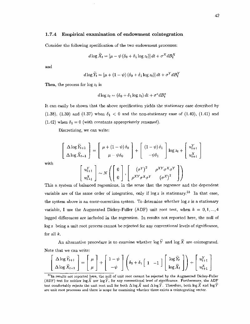
42
1.7.4 E m p i r i c a l e x a m i n a t i o n o f e n d o w m e n t c o i n t e g r a t i o n
Consider the following specification of the two endowment processes:
cflog Xt = \n-fl> (S0 + <Ji log zt)) dt + oxdB?
and
dlog Yt = [/* + (1 - V) (<5o + *i log **)] dt + aYdBY
Then, the process for log zt is
dlog zt = (50 + Si log zt) dt + <jzdBzt
It can easily be shown that the above specification yields the stationary case described by
(1.38), (1.39) and (1.37) when S\ < 0 and the non-stationary case of (1.40), (1.41) and
(1.42) when Si — 0 (with constants appropriately renamed).
Discretizing, we can write:
A l o g F t + i
A log Xt+i
H + (l-i/>)6o
fJL-1p6Q
(l-il>)Si log zt + H+i
H+l
with ut+i
H+l
N 0
0
i°YY pXYaxaY
pXYaxaY (*xy This a system of balanced regressions, in the sense that the regressor and the dependent
variable are of the same order of integration, only if log z is stationary.33 In that case,
the system above is an error-correction system. To determine whether log z is a stationary
variable, I use the Augmented Dickey-Fuller (ADF) unit root test, when k = 0,1,. . . ,4
lagged differences are included in the regression. In results not reported here, the null of
log z being a unit root process cannot be rejected for any conventional levels of significance,
for all k.
An alternative procedure is to examine whether l o g y and logX are cointegrated.
Note that we can write:
A l o g y t + i
A l o g X t + i —
V
•fe +
1 - 1 >
-* SQ + SX 1 - 1
log Ft
logX t
H+l
u: •t+l
33 In results not reported here, the null of unit root cannot be rejected by the Augmented Dickey-Fuller (ADF) test for neither log X nor log Y, for any conventional level of significance. Furthermore, the ADF test comfortably rejects the unit root null for both AlogX and AlogY. Therefore, both logX and logF are unit root processes and there is scope for examining whether there exists a cointegrating vector.

43
This is a Vector Error Correction Model (VECM), with the cointegration vector imposed
to be 1 Without imposing this restriction, the system can be written:
M
. ^ .
+ 1-tp
-1> 60 + 61
Aio g y i + 1
AlogX t + 1
for 7 e R.
I consider the following more general VECM:
r 1
1 7 J logYt
_ logXt _
V +
/
1,Y
ut+l 1,x
. t+1
A l o g F t + i
A l o g X t + i
/
A+T0 1 7 7o
V
logYt
logXt
1
\
)
fc-i
+£r. i = i
A i o g y t _ j + i
A l o g X t _ j + i + u. t+ i
ui
(1.52)
For k = 1, . . . ,4, I estimate the number of cointegrating relationships using the Max
imum Eigenvalue (A-max) and the Trace test statistics, as suggested by Johansen (1988,
1991). For each r, the null hypothesis of both the Maximum Eigenvalue and the Trace tests
is that there exist exactly r cointegrating relationships; the alternative hypothesis of the
former test is that there are r + 1 cointegrating relationships, whereas the alternative of
the latter test is that there are 2 cointegrating relations. The results are presented in Table
1.7. For all lags, the two test statistics indicate that the null of r = 0 cannot be rejected
in favor of either r = 1 or r = 2 for any conventional significance level. However, the two
tests also indicate that the null of r = 1 cannot be rejected in favor of r = 2.
Our empirical results appear to point against the existence of cointegration between
the two (log) endowment processes. However, given the properties of the sample under
consideration (slightly more than 30 years of quarterly observations) and the economic ar
guments in favor of real exchange rate stationarity, a definite answer regarding the existence
and the properties of a cointegrating vector for the two endowment processes is elusive in
this sample.
1.7.5 P r o o f s
Proof of Propos i t ion 1
Let dCt
Ct
E, dCt
Ct = <T?XdB? + <T?YdB} (1.53)

44
and dC: „ fdC! ^-Ei ( | 2 ) = af*dflf + cTYdB( (1.54)
Using (1-6) and (1.8) and applying Ito's lemma, the process of the ratio -^- is:
X J R X , J J O Y
(S) = dri/t + sfdBf + st
r d£/
where
x = s[9^1\(rcx_5(Gtjzl\cx t ~ u \ ^ ut - v \ ™ "t Gt J l \ Gt
SY = 5(Gl^l\aCY_5(G*t-l\^Y
* "x Gt l"1 " \ Gt n J \ W
Applying Ito's lemma to (1.14) and (1.15), we get, respectively:
dlog Ct = drift + acrxdBx + (1 - a)ay'dB? - kt {sXdBx + sYdBf)
dlog C*t = drift + a*oxdBx + (1 - a*)aY dBY + k*t (sxdBx + sY'dBj)
where we have used the following definitions for kt and k%:
a(l-a)A + a*(l-a*)A*(g) /G*x
(aA + a*A* (§-) ) ((1 - a)A+ (1 -a*)A* (%)) V<V
a(l-a)A + a*(l-a*)A* ( g )
(aA + a*A* ( f ) ) ((1 - a)A + (1 - a*)A* ( § ) )
Regarding /c , lim kt = 0 and lim &t = 1. Further, it can be shown that, for the empirically
relevant case 0 < a* < a < 1, kt is globally increasing in ^ - , so it is bounded in (0,1).
Similarly, lim k% = 1 and lim fcjf = 0. For 0 < a* < a < 1, k% is globally decreasing in ^ - ,
so it is also bounded in (0,1).
On the other hand, applying Ito's lemma to (1.53) and (1.54), we get
dlog Ct = drift + <J?XdB? + a^dB?
dlog Ct = drift + cr?*xdBx + a f y' dBj

45
Matching diffusions, we get the following system of equations:
Gt a?X = ~h Gt
A ?x-s(^-)^x
rCY
rc*x
rC*Y
= -kt Gt-l
Gt r?Y
G*t
G*t-l
G*t
+ aay
rC*Y + (1 - a)<7J
= kt
x,Gt-l , o — - — a
ex _ $ I G$ - I \ „c*x
Gt
Gt CY r / Gf ~ I t - a I G,
+ a a
rC*Y *\„Y + (1 - a*)<7
the solution of which is
TCX
rC*x Dct
and
where
,CY
TC*Y
(1 - a) + ((1 - a)k*t + (1 - a*)fc) <5 ( ^ )
Ac [ (1 _ a*) + ((1 - a)k*t + (1 - a*)fct) <J (££1) _
Dc = l + kt5(Gl^\+kt5(
Gt-1
a'
Gt G*t
(1.57)
Proof of Propos i t ion 3
As mentioned in the main text, time t domestic country wealth is the sum of its
appropriately discounted future consumption flows. To calculate domestic wealth in units
of the domestic good, we convert all future good flows in units of the domestic good and
discount using the domestic state-price deflator. Thus
Wt = Et Jt —*
(Xs + Q*SYS) ds
Similarly, to calculate foreign wealth in units of the foreign good we use:
Wt* = Et
/•OO 77* /
Q\ + Y: ds
Using the solutions for S t , EJ, Xt, Yt, Xf, Yt* and Q\, we can calculate the wealth of the
two countries, given in (1.26) and (1.27).
On the other hand the time t value of the domestic country endowment, in units of
the domestic good, is Et r ^sds
Et
/ •OO 7 7
Jt —* Xsds
. After some algebra:
(aX + a*\*)kG + p {aXGt + a*\*G*t)
p{p + k){a\Gt + a*\*G*t) Xt (1.58)

46
To calculate A, we use the fact that, at t — 0, the wealth of each country equals the value (in
units of the numeraire) of each country's endowment. Therefore, for the domestic country,
it holds that
Wo = E0 I =^Xtdt\ Jo —o
Setting t = 0, we can get closed-form expressions for Wo and EQ J0°° s£-Xtdt from (1.26)
and (1-58), respectively. Equating the two expressions, as above, and using the normaliza
tion A + A* = 1, we derive the expression for A given in Proposition 3.
Finally, to derive (1.28), consider that , after substituting the expressions for Wt, W£
and Qt, we get Wt (pGt + kG) A
Wt + W* Q*t (pGt + kG)\+ (PG*t + kG) A*
Setting t = 0 and substituting the expressions for A and A* in Proposition 3, we get (1.28).
Proof of Propos i t ion 4
From (1.47) and (1.48) we get
so, applying Ito's lemma to (1.43) and (1.44) to derive the SDEs that S< and E£ solve and
then taking conditional expectations, we arrive at (1.29) and (1.30).
Proof of Propos i t ion 5
The price of the domestic total wealth portfolio is (in units of the domestic good):
Vt = Et / ^ jt "* Xsds
and, similarly, the price of the foreign total wealth portfolio is (in units of the foreign good):
v: = Et / -Jt " * Yads
Using the expressions for Et, E£, Xt and Ys, we get, after some algebra, (1.31) and (1.32).
Proof of Propos i t ion 6
We can define the diffusion processes of the domestic and the foreign total wealth
portfolio excess return, af- and <r^*, respectively, as the bivariate processes such that
dB% = ^ + Z±dt - r{dt = drift + o-f dB t

47
^ = drift - (axe1 + {uttrf + (1 - w t)of*)) dB*
^ e * = ^ f + £dt - r{*dt = drt / t + a-f'dBt
From (1.31), we can use Ito's lemma to obtain the SDE satisfied by Vt; then, it is easy to
see that the diffusion process of the domestic total wealth portfolio is given by (1.34).
The domestic good market price of risk r]t is denned in (1.47) and, applying Ito's
lemma to (1.43), we get that:
dZt
so, equating diffusions, we get (1.33).
Similarly, applying Ito's lemma to get the SDE for Vf, we get that the diffusion
process of the foreign total wealth portfolio is given by (1.36). An application of It6's
lemma to (1.44) gives
^ = drift - (aYe2 + (u*af + (1 - w t*)of)) dB t
so the foreign good market price of risk, defined in (1.48), is given by (1.35).
Therefore, the excess return of the domestic total wealth portfolio is
dB? = iifdt + <rf dB t
where fif1 is the domestic total wealth portfolio conditional risk premium, calculated as
tf = -±Et(dHZ^)=T&Etr*
Similarly, the excess return of the foreign total wealth portfolio is
dR? = nfdt + o-fdBt
where //£** is the foreign total wealth portfolio conditional risk premium, given by
t,r = -jtEt(d^^=vr^r

Parameter
V
e
</>
log z
a*
a*
pXY
Estimate 0.0037
(0.0006) 0.0520
(0.0204) 0.0195
(0.1436) -1.0348 (0.0243) 0.0074
(0.0007) 0.0195
(0.0018) 0.1553
(0.0786)
Table 1.1: E n d o w m e n t cal ibrat ion
The endowment parameters in (1-37) and (1.38) are estimated by exactly identified GMM,
with moment conditions given in (1.51). The spectral density matrix is Newey-West with 5 lags.
Standard errors in parentheses. Note: the parameters are not annualized.

Endowment parameter Steady-state of endowment ratio z Speed of z mean reversion Endowment growth rate Domestic contribution to endowment adjustment Domestic endowment growth volatility Foreign endowment growth volatility Endowment growth correlation
Preference parameter Domestic preference for the domestic good Foreign preference for the domestic good Subjective rate of time preference Speed of G mean reversion G sensitivity to consumption growth shocks Lower bound of G Steady-state value of G
Symbol z 6
V t/,
ax
aY
pXY
a a*
P k 5 I
G
Value 1
0.192 0.015 0.02
0.015 0.039 0.155 Value 0.990 0.082 0.04 0.12 79.39
20 34
Table 1.2: Calibration parameters
Calibration parameters. All parameters are annualized. The endowment parameters in
Table 1.2 are the annualized counterparts of the parameters in Table 1.1, with the exception of the
steady-state endowment ratio ~z, which is normalized to 1.

50
Moment
Relative endowment value mean
Endowment growth mean
Endowment growth st. dev.
Endowment growth corr.
Endowment growth autocorr.
Consumption growth mean
Consumption growth st. dev.
Consumption growth autocorr.
Consumption growth corr.
Log pricing kernel corr.
Model US UK
8.23 [6.97, 9.47]
1.50% [1.00%, 2.02%]
1.50% [1.31%, 1.69%]
1.50% [0.79%, 2.19%]
3.95% [3.48%, 4.44%]
0.15 [-0.02, 0.32]
-0 .01 [-0.18, 0.16]
1.50% [1.00%, 2.01%]
1.46% [1.25%, 1.68%]
-0 .01 [-0.18, 0.16]
-0 .02 [-0.19, 0.15]
1.50% [0.88%, 2.10%]
2.92% [1.95%, 4.29%]
-0 .02 [-0.24, 0.19]
0.50 [0.20, 0.66]
0.88 [0.72, 0.97]
Data US UK
8.29
1.48%
1.49%
2.01%
3.98%
0.15
-0 .01
1.80%
1.19%
0.33
-0 .29
2.08%
2.05%
-0 .18
0.33
—
Table 1.3: Simulation results: endowment and consumption
A comparison of endowment and consumption simulated and empirical moments. To calcu
late the former, I simulate 10,000 sample paths of the model economy, with each path consisting of
170 quarterly observations. The system is initialized at z\ = z, G\ — G\ = G and Xi = 1. Of the
170 observations, the first 40 (10 years) are discarded to reduce the dependence on initial conditions.
Thus, each sample path consists of 130 observations, as many as available in the dataset. For each
of the moments of interest, Table 1.3 presents the sample average across the 10,000 simulations, as
well as the 2.5% and 97.5% percentiles across simulations (in brackets). The empirical moments are
calculated by using data from 1975:Q1 to 2007:Q2, for a total of 130 quarterly observations.

Moment Model Data
51
Log real exchange rate change st. dev
Log terms of trade change st. dev.
corr(logQ* ,log E)
Openness mean
Corr. of NX with endowment
corr(Aet+i, Ac£+1 - Act+i)
US UK 16.27%
[12.27%, 23.19%] 17.92%
[13.51%, 25.54%]
1.00 [1.00, 1.00]
0.02 [0.02, 0.02]
0.24 [-0.16, 0.60]
0.16 [0.15, 0.18]
0.63 [0.24, 0.88]
0.14 [-0.49, 0.52]
US UK 10.26%
3.75%
0.23
0.02
0.33
0.17
0.28
0.05
Table 1.4: Simulation results: international trade and the real exchange rate
A comparison of international trade and real exchange rate simulated and empirical moments.
To calculate the former, I simulate 10,000 sample paths of the model economy, with each path
consisting of 170 quarterly observations. The system is initialized at z\ = z, G\ = G\ = G and
X\ — 1. Of the 170 observations, the first 40 (10 years) are discarded to reduce the dependence
on initial conditions. Thus, each sample path consists of 130 observations, as many as available
in the dataset. For each of the moments of interest, Table 1.4 presents the sample average across
the 10,000 simulations, as well as the 2.5% and 97.5% percentiles across simulations (in brackets).
The empirical moments are calculated by using data from 1975:Ql to 2007:Q2, for a total of 130
quarterly observations.

52
Moment
Log pricing kernel st. dev.
Equity P/D mean
Equity P/D corr.
Equity excess return mean
Equity excess return st. dev.
Equity excess return corr.
Sharpe ratio
Risk-free rate mean
Risk-free rate st. dev.
Risk-free rate corr.
corr(A log £,.Re)
corr(logE,log(P/D))
Model
US
34.50% [16.81%, 69.53%]
32.10 [27.09, 34.88]
UK
37.09% [19.46%, 73.10%]
31.90 [26.38, 35.14]
0.79 [0.45, 0.97]
6.74% [2.88%, 10.01%]
22.03% [13.95%, 30.90%]
8.46% [3.66%, 12.70%]
25.15% [17.38%, 33.78%]
0.83 [0.69, 0.92]
0.32 [0.11, 0.54] 0.46%
[-1.25%, 3.54%] 1.67%
[0.80%, 3.03%]
0.35 [0.13, 0.58] 0.14%
[-2.66%, 4.09%]
2.01% [1.07%, 3.26%]
0.65 [0.18, 0.93]
0.10 [-0.29, 0.45]
0.13 [-0.58, 0.74]
-0 .40 [-0.72, 0.02]
-0 .39 [-0.88, 0.42]
Data
US
-
40.73
UK
-
25.13
0.94
7.68%
15.53%
7.92%
16.16%
0.69
0.49
1.80%
1.40%
0.49
2.71%
2.52%
0.47
0.00
0.32
-0 .13
0.20
Table 1.5: Simulat ion resul ts : asset prices and r e tu rns
A comparison of asset price and return simulated and empirical moments. To calculate the
former, I simulate 10,000 sample paths of the model economy, with each path consisting of 170
quarterly observations. The system is initialized at z\ = z, G\ = G\ = G and X\ = 1. Of the 170
observations, the first 40 (10 years) are discarded to reduce the dependence on initial conditions.
Thus, each sample path consists of 130 observations, as many as available in the dataset. For each
of the moments of interest, Table 1.5 presents the sample average across the 10,000 simulations, as
well as the 2.5% and 97.5% percentiles across simulations (in brackets). The empirical moments are
calculated by using data from 1975:Q1 to 2007:Q2, for a total of 130 quarterly observations.
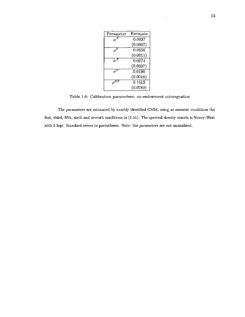
Parameter
M*
MV
ax
ay
pXY
Estimate 0.0037
(0.0007) 0.0050
(0.0011) 0.0074
(0.0007) 0.0198
(0.0018) 0.1512
(0.0780)
Table 1.6: Calibration parameters: no endowment cointegration
The parameters are estimated by exactly identified GMM, using as moment conditions the
first, third, fifth, sixth and seventh conditions in (1.51). The spectral density matrix is Newey-West
with 5 lags. Standard errors in parentheses. Note: the parameters are not annualized.

54
r A-max p — value Trace p — value
k = l 0 1
9.10 0.02
0.28 0.88
9.12 0.02
0.35 0.88
fc = 2 0 1
7.79 0.10
0.40 0.75
7.90 0.10
0.48 0.75
A; = 3 0 1
8.98 0.03
0.29 0.86
9.02 0.03
0.36 0.86
k = A 0 1
9.91 0.00
0.22 0.95
9.91 0.00
0.29 0.95
Table 1.7: Johansen cointegration tests
Results of Johansen cointegration tests for log X and log Y; the econometric specification
is given by (1.52). For the null hypothesis of r = 0 and r = 1 cointegrated vectors, the Maxi
mum Eigenvalue (A-max) and Trace test statistics are presented in the second and fourth column,
respectively; the p-values for each test are presented in the third and fifth columns.

55
Figure 1.1: Empirical probability density functions of surplus consumption ratios
Empirical probability density functions (PDFs). Panel (a) presents the empirical PDF of
the domestic and foreign surplus consumption ratio S = i and S* = 7 - (for the United States
and United Kingdom, respectively). Panel (b) presents the empirical PDF of the ratio -£-
The empirical estimate is calculated by using a normal kernel.
$ •

56
aUSOQ
Figure 1.2: Simulated moments for different values of a
Simulated moments. I examine the sensitivity of model results to the home bias parameters
by fixing a*= 8.2(1 — a), so as to capture the relative openness of the two economies, and vary
the domestic home bias parameter a: a = 0.95 + 0.005.J, j = {0,..., 10}. For each of the values
of a, I simulate 10,000 sample paths of the model economy and, for each of the moments of in
terest, I calculate the sample average across the 10,000 simulations. The horizontal axis measures
the value of a and the vertical axis the value of the moment of interest. Panel (a) presents the
correlation between the domestic and the foreign consumption growth rate, the correlation between
the domestic and the foreign pricing kernel and the Backus and Smith (1993) puzzle correlation
corr(Aet_)_1, Ac£+1— Act+i). Panel (b) presents the standard deviation of: the domestic consump
tion growth rate, the domestic pricing kernel and log real exchange rate changes. Panel (c) presents
the correlation between domestic and foreign risk-free rates and between the excess returns and
price-dividend ratios of the two countries' total wealth portfolios. Panel (d) presents, for each of
the two countries, the correlation: (i) between the excess return of the total wealth portfolio and
the change in the log real exchange rate, and (ii) between the log price-dividend ratio of the total
wealth portfolio and the log real exchange rate.
SDFtxndafcn
Bartu»SrrithaiJ*l ian

57
Chapter 2
Portfolio Choice in Open
Economies with External Habit
Formation
2.1 Introduction
One of the most extensively documented stylized facts in international finance is portfolio
home bias, the overwhelming tendency of investors to hold portfolios heavily skewed towards
assets of their home country. It has long been recognized that portfolio home bias is puz
zling, as it suggests that investors forego significant international diversification benefits.1
Indeed, two of the most prevalent international finance models, the international version
of the Capital Asset Pricing Model (CAPM) and the Lucas (1982) two-country general
equilibrium model, imply that the desire for international risk sharing should lead countries
to hold identical, completely diversified equity portfolios. Extensions of those models that
incorporate frictions and non-tradeabilities have been largely unsuccessful in explaining the
home bias puzzle and, in some cases, have exacerbated the puzzle, suggesting that optimal
portfolios should have a foreign bias.
This Chapter proposes a two-country general equilibrium model in which optimal
risk sharing implies a very high degree of home bias; countries share risk because of, not
despite, portfolio home bias. The key mechanism is novel: home bias results from the
1 There is a long literature on the importance and benefits of international diversification; see, for example, Grubel (1968), Levy and Sarnat (1970), Lessard (1973), Solnik (1974a) and Errunza (1983).

58
desire of investors to hedge against adverse shocks in risk aversion. Agents' preferences
are characterized by external habit formation, which generates countercyclical risk aversion
and, thus, increases the marginal utility of consumption in recessions. Domestic equity is a
better hedge against domestic risk aversion shocks than foreign equity; conversely, foreign
equity is a better hedge against foreign risk aversion shocks. Consequently, domestic agents
hedge their exposure to risk aversion fluctuations by tilting their portfolio towards domestic
equity; foreign investors bias their portfolio towards foreign equity. Furthermore, the model
proposed in this Chapter is able to reconcile international portfolio choice with realistic
asset price dynamics. Given the overwhelming importance of asset return dynamics for
portfolio choice, this aspect of the model satisfies a long-standing need of the general
equilibrium literature in international finance, which has focused on standard preferences
that are unable to match key asset pricing moments.2
The model considered in the Chapter is a two-country general equilibrium model, in
the tradition of Lucas (1982). The global economy is comprised of two countries, Domestic
and Foreign, each populated by a representative agent. There are two goods, the domestic
and the foreign one, and each of the agents is endowed with a Lucas tree that pays continuous
dividends in the country's home good. Each agent has preferences over a home-biased
Cobb-Douglas consumption basket comprised of both goods, so each of the agents derives
more utility by consuming her home good than by consuming the other country's good.
As expected, in equilibrium the home bias in preferences generates consumption home
bias. However, it is not sufficient to generate portfolio home bias; indeed, if preferences
are of the standard CRRA form, there can be a range of portfolios that can support the
competitive equilibrium allocation.3 To generate portfolio home bias, a second assumption
about preferences is crucial: external habit formation. What external habit formation does
is to cause the heterogeneity in consumption, generated by the heterogeneity in preferences,
to give rise to differential hedging demands. In a nutshell, agents do not bias their portfolio
towards the home asset because they want to consume the dividends of that asset; rather,
they want to hold their home country's equity because home equity is the best hedge
against adverse movements in their marginal utility. In fact, in this model, consumption
2Lewis (1999) notes that "[A] major problem with reconciling investor home bias with international consumption movements is that the volatility of the implicit intertemporal marginal rate of substitution is not high enough to explain stock price movements."
3Zapatero (1995) also illustrates that point; he proposes a two-good, two country model with log preferences and shows that, in equilibrium, portfolios are indeterminate.

59
home bias and portfolio home bias are negatively, not positively related: more home biased
preferences generate more consumption home bias, but less portfolio home bias. The reason
is that higher consumption home bias limits the hedging benefits provided by home equity.
Thus, this Chapter shows that it is possible to reconcile portfolio choice with consumption
choice. As expected, the link is through consumption home bias; what may not be expected
is that the mechanism is more complicated than simple intuition may suggest: home bias
in preferences generates deviations from purchasing power parity (PPP) , so that countries
face different investment opportunity sets in real terms, and external habit formation causes
the P P P deviations to generate different hedging demands.
The literature on international portfolio choice and, more specifically, the portfolio
home bias puzzle is extensive. As mentioned above, the canonical models are the inter
national CAPM and the Lucas (1982) general equilibrium model. The key assumption of
both models is that country representative agents are identical, so their portfolio holdings
should reflect that symmetry. In slightly more detail, both models imply that real exchange
rates are constant and P P P holds; the P P P assumption implies that all agents face the
investment opportunity set in real terms, so, if they are identical, country portfolios should
also be identical. Specifically, the international CAPM is a partial equilibrium model which,
taking asset returns as given, leads to the result that the capitalization-weighted world mar
ket portfolio is ex-ante mean-variance efficient. On the other hand, Lucas (1982), from a
general equilibrium standpoint, examines both a barter and a monetary version of a com
plete markets, two-good, two-country endowment economy with no frictions in trade and
finds that the two countries perfectly pool their risks and, as a result, their consumption
growth is perfectly correlated and is financed by holding identical internationally diversified
portfolios.4The reasoning is straightforward: identical agents share consumption risk by
holding the portfolios that allow them to have perfectly correlated consumption growth.
Naturally, the corollary of that reasoning is that differences among country portfolios
can only be generated by relaxing the assumption that countries are identical, so a large
and diverse international finance literature has focused in exploring what kind of differences
between countries can bias investors towards holding their home assets. The literature has
4 Lucas recognizes that the portfolio results of his paper are not empirically validated, mentioning that his result is " [Gjrossly at variance with what we know about the spatial distribution of portfolios: Americans hold a disproportionately high fraction of claims to American earnings in their portfolios, Japanese a high fraction of Japanese assets, and so on."

60
proposed classes of models that relax different assumptions of the standard models. The
first class of models retain the assumption of frictionless financial markets and no arbitrage
opportunities and introduce frictions in the international trade for goods, in the form of finite
or infinite deadweight costs (in the latter case, the literature calls the goods internationally
non-tradeable). Those fictions allow for different equilibrium consumption across countries
and, thus, a non-constant real exchange rate (i.e. P P P deviations). The motivation for those
models arises from the observation that portfolio home bias may be linked to consumption
home bias, the tendency of consumption growth to be highly correlated with output growth
in a given country.5 The reasoning is that differences in equilibrium consumption expose
countries to different consumption risks, so countries have to hold different portfolios in
order to hedge those risks. Under this reasoning, home bias in portfolios can be justified if
domestic assets hedge domestic consumption risk better than foreign assets.
In that vein, Adler and Dumas (1983) modify the international CAPM by proposing
a partial equilibrium model which emphasizes the role of inflation risk. Specifically, they
consider a setup in which agents consume different baskets of goods. In the presence of
P P P deviations, the optimal portfolio for each agent contains an idiosyncratic hedging
component against country inflation and the standard international CAPM does not hold.6
Other models emphasizing the importance of hedging demand for domestic inflation are
Solnik (1974b), Sercu (1980) and Stulz (1981b). However, Adler and Dumas (1983), using
data from 1971-1979, show that hedging portfolios are almost entirely comprised of home
bonds, since risk averse agents prefer to assume some small inflation risk rather than hold
more substantial exchange rate risk. Similarly, Cooper and Kaplanis (1994) show that the
data strongly reject the claim that portfolio home bias can be explained by hedging for
inflation risk.
In a general equilibrium setting, Stockman and Delias (1989) consider a complete
markets endowment economy in which each agent has separable preferences over traded
and non-traded goods; preferences over traded good are identical across agents, while pref
erences over non-traded goods can differ. They show that the optimal domestic portfolio
is comprised by the entirety of claims on the domestic non-traded goods and a diversified
5 See, for example, the argument in Obstfeld and Rogoff (2000). 6 Indeed, they show that the pricing model that emerges is a multi-beta model, in which the riskiness of
each asset does not only depend on its covariance with the world market portfolio, but also on its covariance with each of the individual countries' inflation.

61
portfolio of the claims on traded goods. Thus, consumption and portfolio home bias are
both increasing in the share of non-tradeables in domestic consumption. Baxter, Jermann
and King (1998) consider a generalized version of the Stockman and Delias (1989) model by
relaxing the separability assumption between traded and non-traded goods and show that,
in a world with identical preferences for all agents, each country holds a diversified portfolio
of the claims on tradeable goods, as in the Stockman and Delias (1989) model. However,
regarding the claims on non-tradeable goods, each agent holds appropriate - depending on
the degree of substitutability between traded and non-traded goods - quantities of two other
funds: i) a diversified portfolio of the claims on non-tradeable goods and ii) the claim on
the country's non-traded good. It follows that, under separable preferences, portfolio home
bias is not likely to be justified by the presence of non-tradeables. On the other hand, Tesar
(1993) and Pesenti and van Wincoop (2002) consider partial equilibrium portfolio choice in
economies in which preferences are non-separable and claims on non-tradeable goods are
themselves non-tradeable. Tesar (1993) argues that , under those assumptions, home bias
in the shares of claims on tradeable goods is possible, but Pesenti and van Wincoop (2002)
show that the degree of home bias generated in such an economy would be insufficient to
account for the bias observed in the data.7
Uppal (1993) departs from the assumption of outright non-tradeability and considers
finite trade costs. Specifically, he proposes a complete markets general equilibrium one-good,
two-country model with identical preferences across countries. Although financial markets
are frictionless, there is a proportional deadweight cost when real capital is transferred
internationally. In this economy, investors more (less) risk verse than a log utility investor
bias their portfolios against (towards) home equity, so for realistic levels of risk aversion
the model generates equity foreign bias. The reason is that risk averse agents want to hold
the less risky asset and, due to the negative correlation between exchange rate changes
and foreign equity returns in the model, the less risky asset is foreign equity. Coeurdacier
(2009) confirms that the home bias puzzle cannot be explained by trade costs: he proposes
a two-good, two-country static model with identical preferences across countries and finds
that, for reasonable trade costs, optimal portfolios exhibit a foreign, rather than a home,
7In the same vein, Serrat (2001) proposes a model with heterogeneous preferences and non-tradeables, but Kollman (2006) shows that Serrat's model is characterized by portfolio indeterminacy. The only aspect of portfolio choice that can be pinned down is that, regarding claims to tradeable goods, each agent holds an internationally diversified portfolio.

62
bias.
None of the aforementioned models takes into account labor income. Baxter and
Jermann (1997) argue that domestic human capital returns are highly correlated with do
mestic equity returns and, thus, to hedge against their labor income risk, investors should
hold foreign biased equity portfolios; therefore, the international diversification puzzle is
worse than asset markets suggest.8 However, Heathcote and Perri (2008) show that, in
a two-good, two-country stochastic growth model, domestic human capital growth is neg
atively correlated with domestic equity returns. The reason is that positive productivity
shocks, which generate positive human capital returns, depreciate the domestic good and,
thus, lower the price of domestic equity. Thus, in their model, hedging against labor income
shocks entails holding a home-biased portfolio.
To sum, frictions in the goods market have been unable to generate sufficient port
folio home bias and, in some cases, have exacerbated the puzzle. More forcefully, van
Wincoop and Warnock (2006) show that , under standard CRRA preferences, home bias in
assets cannot be linked to home bias in goods without generating unrealistic results about
asset returns and exchange rates. Partly in response to that failure, other strands of the
international finance literature have proposed alternative sources of home bias. This liter
ature has focused on models that relax either the assumption of frictionless asset markets
or the assumption of full information or full rationality.
The models that examine asset market frictions associated with cross-country in
vesting typically focus on taxes, trading costs and investment restrictions and argue that
frictions may be high enough to wipe out almost all gains from international diversification.
Black (1974) considers the effects of taxation of net foreign investment and finds that such
taxes would lead to significant portfolio home bias. Stulz (1981a) focuses on taxes on gross
foreign investment and finds that domestic investors' risky holdings should be tilted towards
assets with high expected returns, but Kang and Stulz (1997) find that this result is not
supported by Japanese data. Cooper and Kaplanis (1994) propose a model that incorpo
rates deadweight costs of foreign investment and show that, unless risk aversion is much
lower than conventionally thought, the level of deadweight costs that is needed to justify the
empirical levels of portfolio home bias is higher than observable costs, such as withholding
8Julliard (2002) argues that Baxter and Jermann (1997) overstate the advantage of foreign equity over domestic equity for hedging domestic labor income risk, so considering human capital does not necessarily worsen the home bias puzzle.

63
taxes. Furthermore, Tesar and Werner (1995) show that foreign equity investments have
much higher turnover rates than domestic equity investments, so international transaction
costs are unlikely to explain the lack of sufficient international portfolio diversification.
The second class of models emphasize informational or behavioral explanations: do
mestic and foreign investors differ in either their information or their beliefs about the
distribution of asset returns and those differences are such that tilt their portfolios towards
their home assets. French and Poterba (1991) show that the observed levels of portfolio
home bias can be reconciled with mean-variance optimizing behavior only if agents have
very optimistic beliefs about the expected returns of their home assets. To explain their
results, they argue that either agents are indeed overoptimistic about their home assets
or they misperceive foreign assets as excessively risky due to uncertainty. Kang and Stulz
(1997) show that the holdings of foreigners who invest in Japan are skewed towards large
firms and provide some evidence that this large firm bias can be partly explained by the
fact that large firms tend to be better known internationally. Brennan and Cao (1997) also
provide empirical support to the notion of informational asymmetries between domestic and
foreign investors. Van Nieuwerburgh and Veldkamp (2008) show that, if information acqui
sition is not limitless, domestic agents rationally specialize their information acquisition to
domestic securities and, as a result, are less uncertain about domestic assets and tilt their
portfolios towards them.
Apart from being a part of the extensive international portfolio literature, this Chap
ter also belongs to the recent literature that embeds complex preferences in general equilib
rium open economy models, thus bridging the asset pricing literature with the international
finance literature. The model in this Chapter extends the model in Chapter 1, which,
in a complete markets framework, shows how external habit formation can reconcile very
high risk sharing across countries, in the sense of very high pricing kernel cross-country
correlations, with relatively low consumption growth correlations, thus solving the Brandt,
Cochrane and Santa-Clara (2006) international risk sharing puzzle. Both Chapters of this
dissertation build on Pavlova and Rigobon (2007, 2008). They propose a two-country, two-
good model in which preferences are characterized by demand shocks; Pavlova and Rigobon
(2007) assumes complete financial markets, whereas Pavlova and Rigobon (2008) allows
for market incompleteness. Their model is successful in addressing macroeconomic ques
tions, but their assumed preferences are unable to generate realistic asset pricing moments.

64
Verdelhan (2008a) proposes a two-country, one-good model with Campbell and Cochrane
(1999) external habit preferences, while Bekaert (1996) presents a two-country monetary
model which features durability and habit persistence. Moore and Roche (2006) propose a
monetary model with Campbell and Cochrane (1999) preferences and "deep" habits (Ravn,
Schmitt-Grohe and Uribe (2006)). Aydemir (2008) uses a two-country, one-good exter
nal habit model to study international asset prices. Colacito and Croce (2008a, 2008b) and
Bansal and Shaliastovich (2007) study international risk sharing, the forward premium puz
zle and the welfare gains from international portfolio diversification in a two-country Bansal
and Yaron (2004) long-run risks framework. Farhi and Gabaix (2008) examine the asset
pricing implications of a two-country rare disasters model. Lustig and Verdelhan (2006) use
the Yogo (2006) model to explain currency risk premia in a consumption asset pricing set
ting. None of those models examine equilibrium international portfolios, with the exception
of Shore and White (2006), which address the portfolio home bias puzzle with a model that
incorporates external habit formation. In their model, portfolio home bias results from the
attempt of unconstrained investors to mimic, in a "catching up with the Joneses" spirit,
the portfolio behavior of small entrepreneurs, who are forced to hold domestic equity for
agency reasons.
One of the key assumptions of the model proposed in this Chapter is external habit
formation, a preference specification with a long history in economics and finance. The
present work assumes Menzly, Santos and Veronesi (2004) external habits; this specification
shares the motivation of the Campbell and Cochrane (1999) external habit formation model,
but what is assumed is not a process for the surplus consumption ratio, as Campbell and
Cochrane do, but for the inverse surplus consumption ratio.9 The assumption of home
bias in preferences is a common modelling device in international finance; see, for example,
Zapatero (1995).
The model in this Chapter allows for financial market incompleteness. Specifically,
I examine the case no international trade in assets (portfolio autarky). Portfolio autarky
is also considered by Cole and Obstfeld (1991). Other open economy models focusing on
financial market incompleteness include Baxter and Crucini (1995), Kollman (1996) and
Kehoe and Perri (2002), all of which propose models in the international real business cycle
9See Buraschi and Jiltsov (2007), Santos and Veronesi (2006) and Bekaert, Engstrom and Grenadier (2005) for specifications that model the inverse surplus consumption ratio.

65
(RBC) paradigm. In the first two papers, market incompleteness is due to the restriction
that countries can only trade real, non-contingent bonds; in Kehoe and Perri (2002) markets
are incomplete due to the ability of countries to elect to default on their liabilities.
The rest of the Chapter is organized as follows. Section 2 presents the model and
Section 3 describes the equilibrium prices and quantities in a general setting that allows for
market incompleteness. The next two Sections focus on special cases: Section 4 examines
the case of portfolio autarky, while Section 5 the case of complete markets. Section 6
concludes. The Appendix contains the proofs and all supplementary material not included
in the main body of this Chapter.
2.2 The economic sett ing
2 .2 .1 E n d o w m e n t s
The world economy is comprised of two countries, Domestic and Foreign, each of which is
populated by a single risk-averse representative agent who receives an endowment stream
of a single differentiated perishable good: the domestic agent is initially endowed with the
claim on the domestic good endowment, while the foreign agent is endowed with the claim
on the foreign good endowment. Uncertainty in this economy is represented by a filtered
probability space (O,^7 , F , P ) , where F={^ rt } is the nitration generated by the standard
2-dimensional Brownian motion Bt, t € [0, oo), augmented by the null sets. All the stochas
tic processes introduced in the remainder of the Chapter are assumed to be progressively
measurable with respect to F and to satisfy all the necessary regularity conditions for them
to be well-defined. All (in)equalities that involve random variables hold P-almost surely.
The endowment stream of the domestic good is denoted by {Xt} and that of the
foreign good by {Yt}. Both processes are assumed to be ltd processes driven by the 2-
dimensional Brownian shock dBt , satisfying:
dlog Xt = i$dt + crf'dBt
and
dlog Yt = &dt + <r f 'dB t
Both goods are frictionlessly traded internationally, so the price of each good, in
units of the numeraire good, is the same in both countries; in other words, the law of one

66
price holds. Q and Q* denote, respectively, the price of the domestic good and the foreign
good in terms of the numeraire. Without loss of generality, I set the domestic good as the
numeraire good, so Qt = l,Vt G [0,oo). Then, Q* = Q- denotes the terms of trade (the
ratio of the price of exports over the price of imports) for the foreign country and the inverse
terms of trade for the domestic country; in the remainder of this Chapter, Q* will be called
terms of trade without further specification.
2 .2 .2 A s s e t s
Both agents can internationally trade k + 1 assets, k of which are non-redundant risky
assets, with 0 < k < 2. Let the k risky asset returns, in units of the numeraire good, be
given by the /c-dimensional process
d R t = fi.t dt + atdBt
where \xt is the kx\ vector of expected returns and <xt is the kxl asset return diffusion
matrix.
The last asset is locally riskless in terms of the numeraire good and is called domestic
bond. The price of that asset in units of the numeraire is denoted by Dt and solves
dDt = rftDtdt
where rt is the continuously compounded numeraire riskless rate.
Then, we can define excess returns as
d R | = fj%dt + (TtdBt
where fif = fit — rflk, with 1^ representing a kxl vector of ones.
If A; < 2, there are not enough risky assets to span the risk in the economy, so financial
markets are incomplete. For k — 2, financial markets are complete if asset returns are not
perfectly conditionally correlated; in that case the diffusion matrix at is a non-singular
square matrix.
2 . 2 . 3 P r e f e r e n c e s
The domestic representative agent has expected discounted utility
~oo
E0 Je-ptu(XuYt)dt .0

67
where p > 0 is her subjective discount rate, and her instantaneous utility function is
u(Xt, Yt) = \og(XiY?-a ~ Ht) = log(C t - Ht)
where Xt and Yt is the quantity of the domestic and foreign good, respectively, she consumes
at time t, C = XaY1^a is the domestic consumption basket and H is the habit level
associated with that consumption basket. I further assume that the external habit is of
the Menzly, Santos and Veronesi (2004) form. Specifically, it is assumed that the inverse
surplus consumption ratio G = ( QH) solves the stochastic differential equation
dGt = k(G-Gt)dt-6 (Gt " 0 ( f r - ^ ( f r ) ) (2-1)
The inverse surplus consumption ratio is a mean-reverting process, reverting to its
long-run mean of G at speed k and is driven by consumption growth shocks. The parameter
6 > 0 scales the impact of a consumption growth shock and the parameter / > 1 is the lower
bound of the inverse surplus ratio Gt- Obviously, G > I. The local curvature of the utility
function is —U°(C H X'Ct = Gt; for that reason, and in a slight abuse of terminology, in the
rest of this Chapter I will refer to G as domestic risk aversion.
The preferences of the foreign representative agent are similar. Her instantaneous
utility function is
u*(X;,Yt*) = log ( ( X t T * (Yt*)1-11' - Ht) = log(Ct* - H*t)
where Xt* and Y£ is the agent's time t consumption of the domestic and foreign good,
respectively, C* = (X*)a ( y * ) 1 - a i s the foreign consumption basket and H* is the foreign
habit level. Note that home consumption bias for the foreign agent implies a* < 0.5. The
foreign agent's inverse surplus consumption ratio G* satisfies
dG*t =k{G-G*t)dt-5(G*t -V^-Zt^c})) (2-2)
2 . 2 . 4 P r i c e s a n d e x c h a n g e r a t e s
The time t price of the domestic consumption basket C = XaYl~a, in units of the numeraire
good, is
and is defined as the minimum expenditure required to buy a unit of the domestic con
sumption basket C.

68
Similarly, the foreign price index is:
i? = a* / .".* \ 1—a* QA / Qt
Therefore, the time £ real exchange rate, which expresses the price of a unit of the foreign
consumption basket in units of the domestic consumption basket, is:
using the fact that Qt = 1, Vt € [0,oo). When the preferences of the two countries are
identical (a = a*), the two consumption baskets are also identical (C = C*) and have the
same price (P = P*), so the real exchange rate is constant at 1 (absolute PPP) . If the two
countries' preferences differ (a ^ a*), the two consumption baskets are not identical, so
the two countries are exposed to different price shocks. Indeed, the higher the difference in
preferences (i.e. the higher a — a*), the more volatile the real exchange rate.
2.2.5 The agents' problem
As mentioned above, at t = 0, the domestic (foreign) agent is endowed with a claim on
the domestic (foreign) good endowment sequence {Xt} ({Yt}) and nothing else. Since this
claim may or may not be one of the k internationally tradable financial assets, denote by
Nf the real flow, in terms of the numeraire, paid at period t by the non-tradeable part of
the domestic claim. Then:
{ 0, if the domestic claim is tradeable
X-t, if the domestic claim is not tradeable
Similarly, N£ is denned as the real flow, in units of the numeraire, paid each period t by
the non-tradeable part of the foreign claim:
0, if the foreign claim is tradeable
YtQt > if the foreign claim is not tradeable
Let the kxl vector nt describe the investment decision of the domestic agent: the j t h element
of 7Tj describes the amount, in units of the numeraire good, that the domestic agent invests
in the j t h risky asset at period t. Thus, the domestic agent chooses consumption shares Xt
and Yt and investment amounts nt so as to maximize her expected discounted utility
N;
max i?o {Xt,Yt,-"t}
Je~pt log {Ct-Ht)dt o
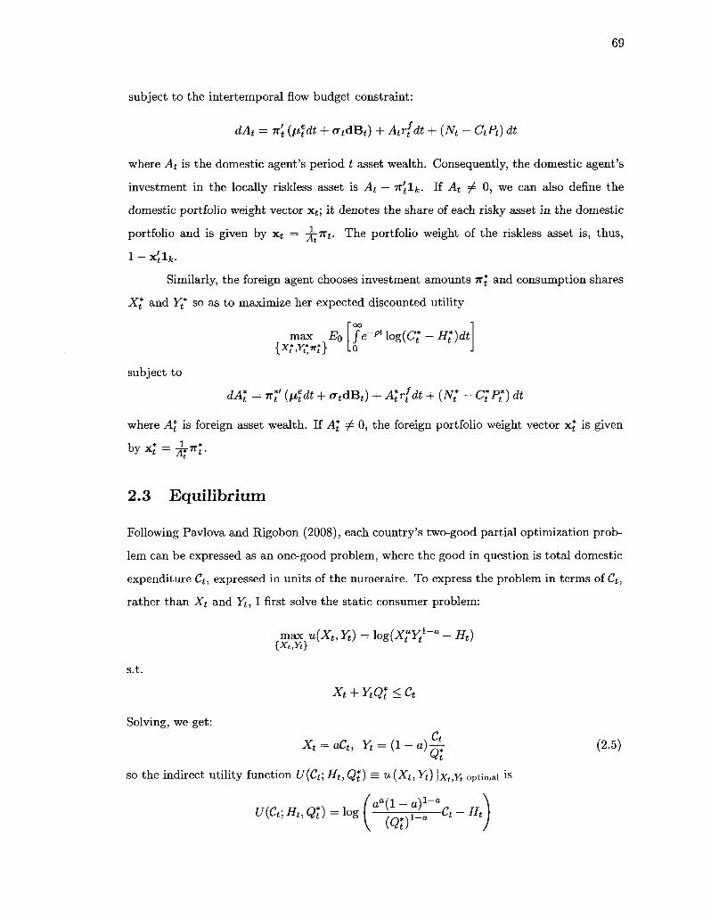
69
subject to the intertemporal flow budget constraint:
dAt = -n't (tfdt + <JtdBt) + Atr{dt + (Nt - CtPt) dt
where At is the domestic agent's period t asset wealth. Consequently, the domestic agent's
investment in the locally riskless asset is At — Tr'tlk- If At ^ 0, we can also define the
domestic portfolio weight vector xj ; it denotes the share of each risky asset in the domestic
portfolio and is given by x t = -j-i^t- The portfolio weight of the riskless asset is, thus,
1 - x£lfc.
Similarly, the foreign agent chooses investment amounts 7r£ and consumption shares
Xf and Yt so as to maximize her expected discounted utility
max EQ oo je-P'logiCt-HDdt o
subject to
dA\ = < (tfdt + atdBt) + A*tr{dt + (Nt* - C*tP*) dt
where A\ is foreign asset wealth. If A\ ^ 0, the foreign portfolio weight vector x£ is given
2.3 Equilibrium
Following Pavlova and Rigobon (2008), each country's two-good partial optimization prob
lem can be expressed as an one-good problem, where the good in question is total domestic
expenditure Ct, expressed in units of the numeraire. To express the problem in terms of Ct,
rather than Xt and Yt, I first solve the static consumer problem:
maxu(Xt, Yt) = l o g ^ Y , 1 " " - Ht) {Xt,Yt}
S.t.
Solving, we get:
Xt + YtQ*t < Ct
Xt = aCt, Yt = (l-a)%; (2.5) Ht
so the indirect utility function U(Ct; Ht, Q$) = u (Xt, Yt) \xt,Yt optimal is
aa(l - a ) 1 " " U(Ct; Ht, Q*t) = log [ " v , ' a Ct - Ht
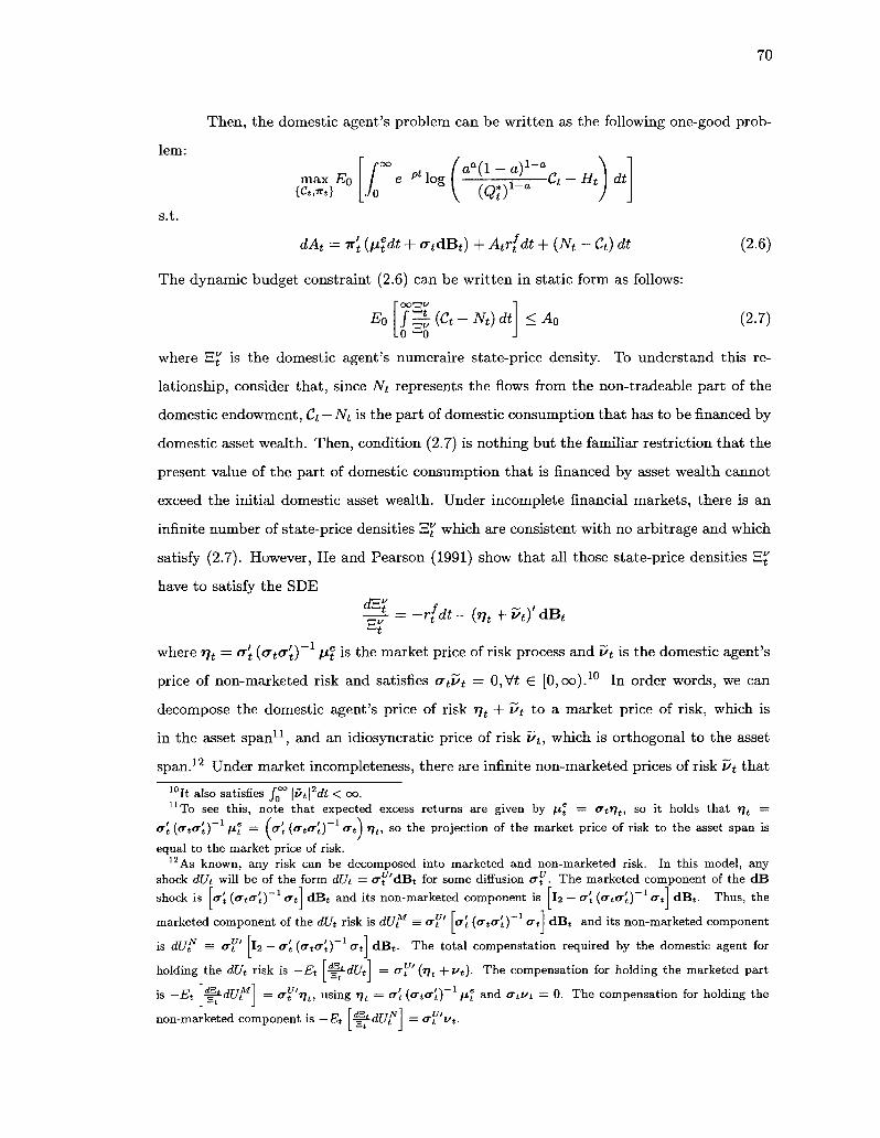
70
Then, the domestic agent's problem can be written as the following one-good prob
lem:
max EQ S:^{^pc,-Hty s.t.
dAt = n't (ntdt + atdBt) + Atr{dt + {Nt - Ct) dt (2.6)
The dynamic budget constraint (2.6) can be written in static form as follows:
Eo f£(Ct-Nt)dt 0 " 0
< A0 (2.7)
where E^ is the domestic agent's numeraire state-price density. To understand this re
lationship, consider that, since Nt represents the flows from the non-tradeable part of the
domestic endowment, Cf — Nt is the part of domestic consumption that has to be financed by
domestic asset wealth. Then, condition (2.7) is nothing but the familiar restriction that the
present value of the part of domestic consumption that is financed by asset wealth cannot
exceed the initial domestic asset wealth. Under incomplete financial markets, there is an
infinite number of state-price densities HJ' which are consistent with no arbitrage and which
satisfy (2.7). However, He and Pearson (1991) show that all those state-price densities E£
have to satisfy the SDE dE?
S---r{dt-(rit + UtyaBt
where r\t = a't ((Tt(r't)~ \i\ is the market price of risk process and v>t is the domestic agent's
price of non-marketed risk and satisfies atut = 0,Vt € [0,oo).10 In order words, we can
decompose the domestic agent's price of risk r\t + Ut to a market price of risk, which is
in the asset span11, and an idiosyncratic price of risk Ut, which is orthogonal to the asset
span.12 Under market incompleteness, there are infinite non-marketed prices of risk v>t that
10It also satisfies Jj°° |£>t[2rf£ < oo.
11 To see this, note that expected excess returns are given by \i\ = <Ttr)t, so it holds that rjt =
cr't (<rtcrt)~ A»t = [cr't {(Ttcr't)~ crA r)t, so the projection of the market price of risk to the asset span is equal to the market price of risk.
12 As known, any risk can be decomposed into marketed and non-marketed risk. In this model, any shock dUt will be of the form dUt = (x^'dBf for some diffusion cr^. The marketed component of the d B shock is \cr't (<Xt<rJ)~ crA d B t and its non-marketed component is I2 — cr't {
(Ttcr't)~ crA d B t . Thus, the
marketed component of the dUt risk is dUt* = &¥' \cr't (crtO't)~ crt dBt and its non-marketed component
is dU? = <TY' I2 — cr't (ct<r't)~ crt d B t . The total compenstation required by the domestic agent for
holding the dUt risk is — Et \^LdUA = cr't' (Vt + v*)- The compensation for holding the marketed part
is — Et ^*dC/ tM = c^'iJt, using r\t = cr't (atcr't)1 Mt an(^ cr* l /t = 0- The compensation for holding the
non-marketed component is — Et l^-dUfl = cr^'i/f
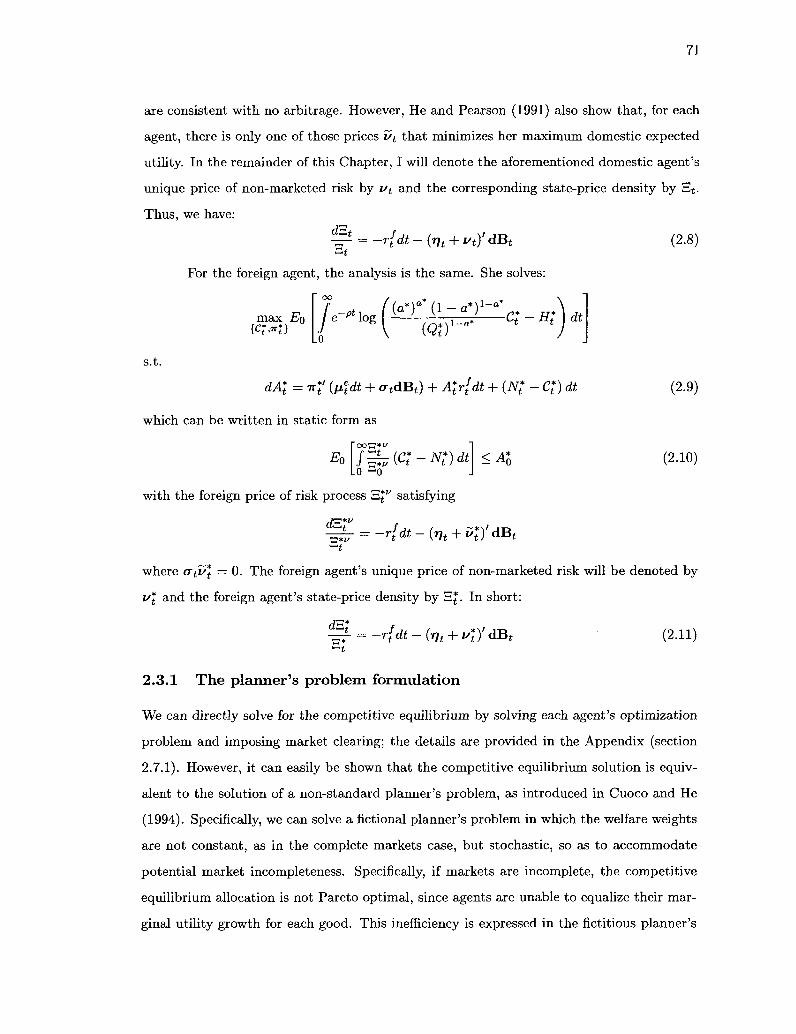
71
are consistent with no arbitrage. However, He and Pearson (1991) also show that , for each
agent, there is only one of those prices vt that minimizes her maximum domestic expected
utility. In the remainder of this Chapter, I will denote the aforementioned domestic agent's
unique price of non-marketed risk by ut and the corresponding state-price density by Et.
Thus, we have:
- r / d t - ( i f c + i / t ) ' d B t St
(2.8)
For the foreign agent, the analysis is the same. She solves:
max EQ / •
.0
-*.o8 w : 1 ' : ? ' ^ ( « ;
v l - a *
s.t.
dA*t = n*t' (rfdt + <7 tdB t) + A*tr(dt + (JVt*
which can be written in static form as
Ht dt
C*t)dt
EQ !^{Ct-N*t)dt L0 " 0
<Al
(2.9)
(2.10)
with the foreign price of risk process "3^ satisfying
d"*v
^±- = -r{dt-(r)t + ulYdBt
where CFiD*t = 0. The foreign agent's unique price of non-marketed risk will be denoted by
v*t and the foreign agent's state-price density by SJ". In short:
^ t _ _ , / J * t - , ..*\'. -r{dt-(rjt + u*t)'dBt (2.11) ^-t
2 .3 .1 T h e p lanner ' s p r o b l e m f o r m u l a t i o n
We can directly solve for the competitive equilibrium by solving each agent's optimization
problem and imposing market clearing; the details are provided in the Appendix (section
2.7.1). However, it can easily be shown that the competitive equilibrium solution is equiv
alent to the solution of a non-standard planner's problem, as introduced in Cuoco and He
(1994). Specifically, we can solve a fictional planner's problem in which the welfare weights
are not constant, as in the complete markets case, but stochastic, so as to accommodate
potential market incompleteness. Specifically, if markets are incomplete, the competitive
equilibrium allocation is not Pareto optimal, since agents are unable to equalize their mar
ginal utility growth for each good. This inefficiency is expressed in the fictitious planner's

72
problem in the form of stochastic welfare weights: the welfare weights are additional state
variables, providing information as to the distribution of wealth at each time.
The fictional planner's problem has the form:
max EQ {Xt,Yt}
oo
je-pt (log(Ct - Ht)dt + \ t log(C t - Ht)) dt
.0
subject to the resource constraints
Xt + X;=Xt and Yt + Y? = Yt
The domestic welfare weight is normalized to 1, whereas the foreign weight is Aj.
It is shown in the Appendix (section 2.7.2) that the competitive equilibrium corre
sponds to a planner's solution with
At = ~ (2.12)
where £ and C* a r e constants. The expression above clearly illustrates that A is the wedge
between the two numeraire state-price densities 2 and 2*.
In more detail, consider the fictitious representative agent and note that, at period t
U(XU Yt- At) = max {u(Xt, Yt) + \tu{X*t ,Yt*)} Xt+X;=Xt,Yt+Y?=Yt
so
or
8U(Xt,Yt) _ du(Xt,Yt) = du{X*t,Yt*)
dXt 9Xt * dX*
du(Xt,Yt)
Xt dXt du(x;,Yt*)
exi
Similarly, for the foreign good it holds that:
dU(Xt,Yt) du(XuYt) du(X;,Yt*)
dYt 9Yt dYt
or du(Xt,Yt)
Xt = dYt
du(x:,Yt') 8Y*
In other words, the stochastic welfare weight A represents the wedge that financial
market incompleteness introduces to the two agents' marginal utility growth. In complete
markets, A is constant: perfect risk sharing stipulates that marginal utility growth is equal
ized across agents. When markets are incomplete, though, there are not enough assets to
efficiently share risk and marginal utility growth cannot be equalized across agents.

73
Furthermore, the foreign welfare weight A is connected to the wealth distribution
between the two countries. Specifically, define as domestic aggregate wealth W the present
value, in units of the numeraire good, that future consumption expenditure has for the
domestic agent (i.e. the value calculated by applying the domestic state-price density £ ) :
Foreign wealth W* is denned similarly:13
w; = Et
007?
J-^-Csds
JBC*sdS
t " t
The following proposition, proven in the Appendix, clarifies the relationship between wealth
and welfare weights.
Proposi t ion 7 Domestic wealth, in units of the numeraire good, is
* aGt + a*\tG*t p{p+k) y ' ;
and foreign wealth, in units of the numeraire good, is
Wt = A ^ ?G*+k° (2.14) 4 aGt + a*XtG*t p(p + k) K '
Therefore, pGt + kG Wt*
M = pG\ + kG Wt
We can easily see that the welfare weight A is partly representing the ratio of the two
countries' wealth; under this interpretation, the higher A is, the more wealthy the foreign
country is. However, it would be more accurate to discuss A not in terms of wealth, but in
terms of welfare. In that sense, A represents the conditional welfare gain or loss that the
foreign agent experiences. Under incomplete markets, the two agents cannot completely
share risk; the two agents have to take different risks. A high A characterizes a state of the
world in which the foreign agent has low marginal utility - and, thus, high utility - because
the idiosyncratic risks she has taken have had a positive outcome. This may or may not
mean that the agent is wealthier; all it means is that the agent has taken idiosyncratic risks
13Note that, if markets are incomplete and the densities H and E* differ, then, under the definition used here, the two countries may reach different valuation conclusions for each country's wealth. In that sense, wealth, as defined here, is a local, rather than a global, measure.

74
that ex post paid off. This is exactly the meaning of a higher planner's welfare weight: a
high A means that the foreign agent is better off in welfare terms.
Using (2.8), (2.11) and (2.12), a characterization of the stochastic process A can be
easily obtained; it is presented in the following lemma.
L e m m a 8 The foreign welfare weight process A satisfies
^ = {v*t-ut)'u*tdt+{ul-ut)'dBt
In the complete markets case, all economic risk is marketed, since there are enough
assets to span all risk, so crt is non-singular and vt = u\ = 0,W € [0,oo); in that case,
At = Ao = A. However, under incomplete markets, non-marketed risk is priced differently
by the economic agents, so differences in the price of non-marketed risk (u^—vt) affect
equilibrium prices and quantities. In that case, to fully characterize the behavior of A we
need to solve for the idiosyncratic prices of non-marketed risk v and u*. For that, we need,
in turn, to solve for the asset return diffusion matrix a, so that we can identify the asset
span and, thus, the marketed risk space. Thus, as expected, the behavior of the fictional
welfare weight A depends on the structure of international asset markets - in other words,
on which assets are internationally tradeable.
2 .3 .2 Q u a n t i t i e s a n d pr ices
In this section, we characterize all quantities and prices of interest in terms of the five
state variables X, Y, G, G* and A; of course, the latter state variable is non-trivial only
when financial markets are incomplete. Under market incompleteness, the conditional cross
country distribution of wealth, as encapsulated in the value of At, affects equilibrium prices
and quantities; thus, under incomplete markets, the divergence of equilibrium prices and
quantities from their complete markets counterparts depends on the divergence of the con
ditional value of A from its constant, complete markets, value.
2.3.2.1 Macroeconomic quantit ies and prices
The domestic equilibrium consumption allocation is
Xt = utXt, Yt = uJ*tYt (2.15)

75
and the foreign consumption allocation is
x; = (l-ut)Xt, Yt* = {l-u*t)Yt (2.16)
where I introduce the share functions u>t and u\
ut = w ( At, — 1 = v ^ r v
UJf — U) [At —
'G*J ( l - a ) + ( l - a * ) A t ( f )
with uit (u>l) being the proportion of domestic (foreign) endowment consumed domestically.
Naturally, in the case of complete home bias (a = 1, a* = 0), u)t = 1 and u;£ = 0, Vt 6 [0, co),
since each country consumes its endowment. Both share functions are decreasing in the
welfare weight At; the higher the foreign welfare weight At, the more of the world endowment
is consumed by the foreign country. This effect makes economic sense: since \ t is a rough
proxy for the relative wealth of the foreign country, it stands to reason that higher At,
implying a relatively wealthier foreign country, leads to an elevated foreign consumption
share. More importantly, both share functions are decreasing in the ratio ^ - ; in other
words, an increase in a given country's risk aversion increases its consumption share for
both goods. This is due to risk sharing; when a country is in a bad state of the world and
its risk aversion is high, it needs to consume more, as its marginal utility of consumption is
higher.
Trivially, domestic consumption expenditure is given by
Ct = 1—F^\Xt (2-17)
and foreign consumption expenditure by
c ? = — G t L \ X t (2-18) a + a*At(^J
c* Domestic (foreign) consumption expenditure is decreasing (increasing) in both At and -^-.
Furthermore, domestic consumption is
Ct = uat{u*t)
1-aX?Yt1-a (2.19)

76
and foreign consumption is
CI = (1 - cotf (1 - uD^'xf Y?~*' (2.20)
The terms of trade are given by
( l _ o ) + ( l_a .)A t(gW «* = /o-\ V (2-21)
Under home bias (a > a*), the price of the foreign good, in units of the numeraire, is
increasing in the welfare weight At. The reason for this is that an increase of foreign
country wealth when the foreign country is home biased implies a relative increase of the
demand for the foreign good, pressuring its relative price upward. Furthermore, the terms c*
of trade are increasing in -^f-; high foreign risk aversion implies high foreign consumption
demand and, thus, due to home bias, a high relative price for the foreign good.
Finally, the domestic trade balance (domestic net exports) is given by
TBt = Xt- CtPt = Xt - YtQ*t = ( l - ^ ) Xt
Since ut is decreasing in At, TBt is increasing in At. This also makes economic sense: when
the foreign country is wealthier, it consumes more of the global goods endowment. The
only way for the foreign country to increase its consumption is to increase it net imports -
which translates to higher net exports for the domestic country.
2.3.2.2 The pricing of risk
The price of numeraire risk for each of the two agents is given by their numeraire state-price
densities E and 3*; they are their discounted marginal utilities for the domestic good. The
numeraire state-price density of the domestic agent, 3 , is
- = e - „ i . G , + y A , G ; (222)
C Xt
while the numeraire state-price density of the foreign agent, 3*, is
(2.23) _ot 1 1 aGt + q*AtGt*
C* At Xt
Both marginal utilities are increasing in conditional risk aversions G and G*; the marginal
utility of consuming the numeraire good is higher when either the domestic or the foreign

77
risk aversion are high. Furthermore, both S and S* are decreasing in X; for both agents,
the marginal utility of the numeraire good is proportional to its scarcity. The result is that
both agents require high compensation (in the form of expected return) from assets that
have low payoffs when either risk aversion is high or when the state of nature is unfavorable
(low endowment realization).
Where the behaviors of S and S* diverge is with respect to the welfare weight A: the
domestic state-price density S is increasing in A, whereas the foreign density 5* is decreasing
in A. This result has a natural economic interpretation: high values of A correspond to states
of nature in which the foreign agent is relatively wealthy and the domestic agent relatively
poor, so the marginal value of the numeraire good is high for the "poor" domestic agent and
low for the "rich" foreign agent. This difference in the behavior of the two agents' state-
price densities introduces differences in the pricing of numeraire good flows. Specifically,
each agent is willing to pay a high price for flows negatively correlated with her wealth. In
other words, numeraire flows that are positively correlated with foreign relative wealth A
are valued more highly by the domestic agent than the foreign agent; the opposite is true
for flows that are negatively correlated with A.
2.3.3 Consumption volatility and risk sharing
Having described the levels of the variables of interest, in this section we focus on cross
country risk sharing, which entails characterizing the conditional variance of consumption
growth rates. The following proposition, proven in the Appendix, sheds lights on equilibrium
consumption risk.
Proposi t ion 9 The equilibrium consumption process for the domestic representative agent
i s ^ - E t (j%) = crf'dBt, with
°f = -fi-c H f + (! - a)°f)
+ c { [(«*** + O °? + ((1 - «*)** + (! - *)*?) "t] * (^f) }
and the equilibrium consumption process for the foreign representative agent is -^-—Et I -gi-)

78
c r f ' d B t , with
*? = ^ («V + (1 - a>D
+^~c { [(a*fet + ak*t) af + ((1 - a*)h + (1 - a)fc*) o f ] 5 ( % p ) }
where kt, k^ and D% are functions of Gt, G$ and At defined in the Appendix (equations
(2.37), (2.39) and (241), respectively).
Denoting the consumption growth diffusion process in the complete markets case by
a^ and a^ , for domestic and foreign consumption growth, respectively, the incomplete
markets solution can be written as:
^ = **C-^W-"*)
and
at =(Tt + JjE \ut ~ut)
Domestic (foreign) consumption growth volatility is decreasing (increasing) in the price
difference of non-marketed risk v\— ft\ for each of the agents, higher compensation to
bear non-marketed risk is associated with higher consumption growth risk relative to the
complete markets benchmark.
2.4 The portfolio autarky case
In this section, I assume that no financial assets can be traded internationally; the only
trade between countries is trade in goods. Trivially, this implies that the each country's
trade balance is always identically zero: the value of each country's imports need to equal
the value of its exports. Furthermore, since with no asset trade the current account is equal
to the trade balance, both countries' current accounts are always zero. Thus:
TBt = TB*t = CAt = CA*t = 0, Vt 6 [0, oo)
In this setup, there is no portfolio decision. The domestic agent chooses {Xt,Yt}
to maximize her expected discounted utility under a set of zero trade balance constraints.

79
Thus, for the risky assets, izt = 0 = -K\. Since no bonds are traded, we also have At—7rjlfc =
0, so At = 0 and, similarly, A*t = 0. Therefore, the domestic agent's problem is:
max EQ {x,Yt}
fe-**log(X?Y?-a-Ht)dt o
such that domestic trade balance is zero at each time t:
Xt + YtQt = Xt
Similarly, the foreign agent maximizes her expected discounted utility under the zero trade
balance constraint Xf + Yt*Qt = YtQt-
It can easily be determined that the competitive equilibrium allocation is
Xt — aXt and Yt = a*Yt
for the domestic agent, and
X; = (1 - a) Xt and Yt* = (1 - a*) Yt
for the foreign agent.
Since the equilibrium allocation differs from the complete markets allocation, market
incompleteness implies a welfare loss for the agents, caused by their inability to use financial
markets in order to efficiently share risk. This also implies that the two agents' marginal
utility is not equalized. Indeed, the domestic agent's state-price density is
<Xt
where the foreign state-price density is
"* C* 1 - a Xt
Thus, the wedge A between the two densities is
* - ^ § <2'24> The fictional welfare weight A adjusts in a way that represents the impact of imperfect risk
sharing to consumption and, thus, welfare. Without asset markets, the shock in domestic
risk aversion G, given by ^ — Et ( ^ J, satisfies

80
so it is a home-biased weighted average of the domestic and the foreign endowment shock.
To clarify ideas, assume, for example, that domestic endowment shocks have been mostly
negative in the recent past, whereas foreign endowment shocks have been mostly positive.
Then, due to home bias, domestic consumption shocks have been mostly negative, while
foreign consumption shocks have been mostly positive. Since negative consumption shocks
imply positive shocks in risk aversion, Gt > G$: the country which has experienced mostly
negative consumption shocks is more risk averse than the country that has experienced
positive shocks. This is not surprising: since countries cannot efficiently share risk, home
bias implies that each country has to shoulder most of the burden of unfavorable realizations
of its home good endowment process.
The differential welfare of the two countries, given those shocks, is expressed by the
fictional welfare weight A. In the case we consider, A will be above its steady-state value,
illustrating the fact that the foreign country is "wealthier", in the sense that it consumes
more than it would consume in the complete markets case. Indeed, under complete markets,
the domestic country would have insured itself against adverse relative shocks in a way that
keeps A constant. Without financial assets, on the other hand, each country has to bear
most of the burden of bad realizations of its endowment. The welfare weight A measures
exactly this burden; in complete markets, allocations are a function of the risk aversion ratio
^ j - , since Pareto optimality dictates that consumption should shift to the conditionally
more risk averse country. Without assets, however, the link between consumption and
the risk aversion ratio is broken, since countries cannot efficiently allocate risk - in that
regime, consumption only depends on endowment realizations. Thus, the welfare weight A
completely eliminates all the dependence of the consumption allocation on the ratio -Q .
To examine the properties of equilibrium prices and quantities in the portfolio au
tarky setup, I simulate 20,000 sample paths of the model economy, each consisting of 200
quarterly observations (50 years), for different degrees of preference home bias.14 I specify
that both endowments follow a Geometric Brownian motion, so that \ix = fxx, fi^ = fJ-x,
ax = [ax 0]' and ax = [0 <JY}'\ this implies that endowment growth is uncorrelated across
countries.
The system is initialized at the steady state {G\ = G\ = G) and I adopt the
14To reduce the dependence on initial conditions, for each of the 20,000 paths I generate a time series of 240 quarterly observations (60 years) and eliminate the first 40 observations (10 years).

81
normalization X\ — Y\ = 1. The calibration is symmetric; the annualized parameter
values used are as follows: p = 0.04, k = 0.12, S = 79.39, G = 34, I = 20, // = 0.015,
<TX = <ry = 0.015 and pXY = 0.15 I consider domestic home bias parameter values of
a = 0.5, 0.7, 0.9, 0.95, 0.99 and 1. For each of the values of a, a* = 1 — a, so the degree of
home bias is identical in the two countries.
Table 2.1 presents the properties of several key moments in this economy. Due
to symmetry, consumption growth and pricing kernel volatility are virtually identical in
the two countries for all levels of home bias. As expected, the less divergent are the two
countries' preferences, the higher the correlation of their consumption growth and marginal
utility is. Due to home bias, the agents take different amounts of each risk, so they price
them differently. The domestic agent is more exposed to domestic endowment shocks,
so she prices domestic endowment risk higher than her foreign counterpart: for all home
bias parameterizations, the first element of the v*—v vector, {u*—u)v which denotes the
cross-country difference in the price of domestic endowment risk, is (weakly) negative. The
opposite is true for foreign risk: (i/*—i/)2 is always weakly positive. The two agents price
the risks identically only when a = a* = 0.5, in which case they have the same preferences
and, thus, perfectly pool all risks.
2.5 The complete markets case
In this section, I assume that both endowment claims are internationally tradeable: the
agents can trade the domestic total wealth portfolio and the foreign total wealth portfolio:
the domestic (foreign) total wealth portfolio is the asset that pays as dividend, each period,
the endowment of the domestic (foreign) good. The net supply of each of those two assets
is normalized to one. The period t price of the domestic (foreign) claim, in units of the
domestic (foreign) good, is denoted by Vt (Vt); thus, the numeraire price of the domestic
asset is Vt and that of the foreign asset is V^Qt- All returns are expressed in units of the
numeraire good.
Recall that both agents can also trade the domestic bond, which is locally riskless
15 The mean and standard deviation of endowment growth are set equal to the correspoding moments of quarterly US endowment growth from 1975:Q1 to 2007:Q2, with endowment defined as the sum of consumption of non-durables and services and net exports. The habit parameters are those used in Menzly, Santos and Veronesi (2004), with the exception of k, which is set slightly lower. The calibration here follows the calibration in Chapter 1.

82
in terms of the numeraire. Thus, both agents have access to two risky assets (the two total
wealth portfolios) and one riskless asset (the domestic bond).16
Since both endowment claims are marketed, the analysis presented in the previous
section applies with Nt = JVt* = 0.
Since there are two risky assets (k = 2) and two sources of risk in the world econ
omy, financial markets are potentially complete; they are incomplete only if the conditional
returns of the two assets are perfectly correlated. The following proposition illustrates that ,
unless the two countries have the same preferences (q = a*), trading in the two endowment
claims is sufficient to dynamically induce market completeness. In that case, the welfare
weight is constant: Xt = A,Vt € [0,oo).
Proposi t ion 10 If a ^ a*, the asset return diffusion matrix <Tt is non-singular. Then,
Vt = v\ = 0 and financial markets are complete. If a = a*, the two total wealth portfolios
have perfectly correlated returns in terms of the numeraire good, so art is singular.
In the rest of the section we will focus in the complete markets case a^ a*.
2.5.1 Equilibrium portfolios
Equilibrium portfolios are given by the following proposition, proven in the Appendix.
Proposi t ion 11 For a ^ a*, the domestic country equilibrium portfolio weights are given
by xt = [xY ,xY ]' where
v _., (a + a*\)kG + apGt + a*pXGj
[a - a*) [kG + pGt)
and
xT = l-xY (2.26)
while the foreign country equilibrium portfolio weights are given by x£ = [x^v, x1[v']' where
*v n , (a + a*X)kG + apGt + a*p\G*t Xt = - ( 1 _ a ) {a-a*)X{kG + PGt) (2-27)
We could also introduce a foreign bond, an asset that is locally riskless in terms of the foreign good. Due to terms of trade risk, this is a risky asset in terms of the numeraire. Since there are only two sources of risk in the world economy, if the two total wealth portfolios have linearly independent returns, then the two assets induce market completeness and the foreign bond is a redundant security; its payoffs can be replicated by a portfolio consisting of the domestic total wealth portfolio and the foreign total wealth portfolio. As it will be shown shortly, this is true for a ^ a ' , s o w e can ignore the foreign bond.

83
and
x?* = l-x? (2.28)
The domestic agent holds a fixed portfolio comprised of6Y = *!"! = 9V shares of the domes
tic total wealth portfolio and 9t = — a°La, = 9 shares of the foreign total wealth portfolio.
Consequently, the foreign agent holds a fixed portfolio comprised of 9\ — — ^ l = 9
shares of the domestic total wealth portfolio and 9% = _f . = 9 shares of the foreign
total wealth portfolio.
The first important point is that, in equilibrium, no country holds domestic bonds.
Furthermore, each country's equilibrium portfolio is comprised by a constant number of
shares: both agents adopt a buy-and-hold strategy and never reallocate. In fact, under home
bias (a > a*), each country holds a long-short portfolio: each country holds a leveraged
position in its own asset, financed by short-selling the other country's asset; for the domestic
portfolio, 6V > 1 and 9V* < 0, and for the foreign portfolio, 6*v < 0 and 9*v* > 1 .
Equilibrium portfolios are not just home biased, they are superbiased.17 However, although
the amount of shares in each country's portfolio is constant, the portfolio weights x< and x£
are time-varying: an increase in domestic risk aversion G leads both countries to reallocate
their portfolio towards the foreign asset, while an increase in G* induces reallocation towards
the domestic asset for both countries; this is the result of valuation effects, explained in more
detail below.
To understand those results and to clarify the elements introduced by external habit
formation, it is useful to consider the benchmark of an economy without habits, keeping
everything else the same. Under standard log preferences over a home biased Cobb-Douglas
consumption basket, each country consumes a fixed proportion of the endowment of each
good. In that economy, the only risk present is endowment risk: fluctuations of the two
endowments X and Y. Equivalently, we can consider the relative endowment z = -£ and
write the two endowments as X and z X . Using this formulation, we can see that, in this
setup, risk sharing refers to the sharing of relative endowment risk; fluctuations in X in
effect represent undiversified global risk. This is evident when we consider the consumption
expenditure for each of the countries: domestic expenditure is Ct = Xt, while foreign
expenditure is C\ = {^pr) Xt, so equilibrium expenditure is perfectly correlated across
17 The possibility that Cobb-Douglas heterogeneous preferences across countries could give rise to super-biased portfolios is examined in Bennett and Young (1999).

84
countries and is exposed only to global risk X and not to relative endowment risk z. It is
important to note that the diversification of relative endowment risk z is achieved through
fluctuations of the terms of trade. For example, when a positive shock increases the domestic
endowment, a proportional reduction in the relative price of the domestic good leaves the
consumption expenditure of both countries completely unaffected. Thus, international trade
in goods leads to the perfect sharing of relative endowment risk. Naturally, this eliminates
the need for risk sharing through financial markets: international trade in goods is sufficient
for Pareto optimality. In fact, financial markets are not complete in this setup, since the
terms of trade fluctuations also induce perfect correlation in (numeraire) asset real flows.
Specifically, at period t, the domestic asset pays numeraire flows of Xt, while the foreign
asset pays numeraire flows of Yt Q\ = -jj^Xt, so one of the two assets is redundant and the
competitive equilibrium allocation can be achieved by any buy-and-hold portfolio 9 ,9
that satisfies 9V + ^r9v = 1- However, this market incompleteness does not matter
for welfare purposes, as asset trading is not necessary. Note that the aforementioned set
of portfolios includes both the habit equilibrium portfolio 1 ~ at , — ^ - j - and the autarky
portfolio [1,0]. Furthermore, since countries can achieve Pareto optimality by trading in
the spot market for goods, they can gain no risk sharing benefits through current account
fluctuations. Indeed, both the trade balance and the current account are identically zero at
all periods for both countries.
In the habit economy, countries trade assets in equilibrium. Specifically, their be
havior is very straightforward: each country holds a static portfolio which, each period,
pays exactly the amount of resources that the country needs in order to afford its Pareto
optimal consumption allocation. Then, each country achieves that allocation by trading in
the spot market for goods. For example, each period the domestic country portfolio pays
dividends of 9vXt units of the domestic good and 9V Yt units of the foreign good; those
dividends are worth 9 Xt + 9 YtQt numeraire units. What the domestic country needs
to consume - Xt units of the domestic good and Yt units of the foreign good - is worth
Xt + YtQt numeraire units, so the domestic agent has exactly the resources she needs to
buy that consumption bundle: 9vXt + 9v*YtQ\ = Xt + YtQt- All t n e domestic agent has
to do to achieve the desirable allocation is to exchange 9 Xt — Xt > 0 units of the domestic
good for Yt — 9v*Yt > 0 units of the foreign good in the time t spot goods market. It is
notable that, with the exception of period t = 0, the countries do not need to trade assets

85
in order to share risk; the only trading that takes place is in the spot market for goods.
This intratemporal - rather than intertemporal - risk sharing behavior is further illustrated
by the fact that countries do not hold any bonds at all.
Naturally, this behavior leads to current account balance at each period, as the
countries do not need to smooth consumption by moving wealth across time. Formally,
recall that the domestic current account CA is comprised of the sum of the domestic trade
balance and the net flows (dividends and interest payments) from the domestic net foreign
portfolio. Thus:
CAt = TBt + (oY'YtQt - OfXt) = TBt + ( ^ - l ) Xt = 0
In the complete markets case, net foreign portfolio flows completely counterbalance net
trade flows; although the domestic trade balance is non-zero, the current account is always
zero. Trivially, the foreign current account is also identically zero: CA\ = 0, Vt G [0,oo).
The long-short nature of equilibrium portfolios is motivated by the need to hedge
against risk aversion fluctuations. In contrast to the simple log economy analyzed above,
the marginal utility of the agents in the habit economy also depends on conditional risk
aversion G and G*. Risk sharing is achieved by consuming time-varying shares of the global c*
endowments: recall that domestic expenditure Ct is decreasing in -^-. This is due to risk
sharing: relatively high domestic risk aversion pushes domestic marginal utility upwards,
so marginal utility growth can be equalized across countries only if the domestic country
consumes more. Since domestic consumption is decreasing in ^ - , the domestic agent needs c1*
to hold a portfolio that is a good hedge for fluctuations in -^-, so that it can finance
her consumption. The numeraire cashflows of the domestic asset are Xt, while those of
the foreign asset are YtQt = ^aG*+am~\G*—^-^t, positively correlated with -^-. In other
words, for the domestic agent, the domestic asset is a better hedge than the foreign asset.
To be more precise, the reason the domestic asset is a hedge for the domestic asset and
risky for the foreign agent is due to the behavior of the terms of trade (and thus the real
exchange rate). Under home bias, the terms of trade Q*t are increasing in -^-, so the foreign
good become cheaper exactly when the domestic agent is very risk averse and needs high
consumption; for the domestic agent, holding the foreign asset is very risky. Exactly the
opposite is true for the foreign agent. This heterogeneity between the two agents, generated
by their home biased preferences, leads to the formation of long-short equilibrium portfolios.

86
To see the effects of investor heterogeneity in portfolio choice, we can decompose each
agent's equilibrium portfolio in a mean-variance efficient portfolio and a hedging portfolio;
the former is common for both agents, but the latter differs, due to differing preferences.
The decomposition is given in the following lemma, the proof of which can be found in the
Appendix.
L e m m a 12 The equilibrium risky portfolio for the domestic agent can be written as
x t = {van (dR?))-1 Et (dRf) + { ^ ~ ) {vart (dRf J)"1 covt ( d R | , ^ )
and the optimal risky portfolio for the foreign agent can be written as
xt* = {van ( d R ? ) ) - 1 Ek ( d R | ) + ( p g f ^ f c ( g ) (^n ( d R f ) ) " 1 covt ( d R | , ^
The conditional mean-variance efficient portfolio is {van ( d R f ) ) - Et (dRf) and is
common for both agents, while hedging portfolios are agent-specific. Specifically, the do
mestic hedging portfolio is the projection of domestic risk aversion shocks to the asset
span and, thus, is maximally conditionally correlated with shocks in domestic risk aversion.
It follows that the domestic hedging portfolio provides the maximum possible insurance
against increases in G. The analysis is similar for the foreign agent; her hedging portfolio
is the portfolio that is maximally correlated with shocks in G* and, thus, provides the best
possible insurance against increases in G*.
It is important to note that the each agent's hedging demand for each individual
asset does not depend only on that asset's hedging properties, but also on the hedging
properties of the other asset and the covariance of the assets' returns. The signs of hedging
demands are given by the following corollary.
Coro l l a ry 13 The mean-variance optimal holding of the asset i is 1 corrt( ^H' t> *
where SR\ is the time t Sharpe ratio of asset i. Furthermore, the sign of the domestic hedging
demand for asset i is given by the sign of corrt ( dR\, ^f- J —corrt ( dR3t, -^ J corrt (dR\, dRJ
t J,
while the sign of the foreign hedging demand for asset i is given by the sign of corn \dR\, -Q^) —
corn (dRl, -Q£- ) corrt \dR\, dRj ) , i ^ j .
Therefore, the mean-variance optimal portfolio, common to both agents, depends
heavily on the Sharpe ratios of the two assets. Regarding the hedging portfolio, an agent

87
can maintain a positive hedging demand for an asset that has poor hedging properties if the
alternative is to hold even worse hedging instruments; on the other hand, the agent may
short a good hedge if she can use that short position to finance a large long position in an
even better hedge.
2.5.2 Home bias
The static nature of countries' portfolios does not mean that equity home bias is constant;
home bias will be time-varying, due to valuation effects. To see this more clearly, define
domestic home bias as:
Value of domestic holdings of foreign assets rr ry -. Value of total domestic holdings Mrft = 1 Total value of foreign assets
Total value of world assets
When the domestic agent invests in foreign assets in proportion to their market capitaliza
tion, the home bias measure takes the value of 0; this is the case of no home bias. When the
domestic agent invests solely in domestic assets, then the above measure takes the value of
1; the domestic agent is completely home biased. Here, we have:
ev*v,*Q*t
Vt+Vt*Q*t Vt+Vt'Q*t L - a - a ^ Vt )
Under home biased preferences (a > a*), the degree of domestic home bias is time-varying V*Q*
solely because the relative valuation term fv * is time-varying. The end result is procyclical
home bias: domestic home bias is more pronounced when the domestic economy is in a
relative expansion. More specifically, domestic home bias is increasing in two variables: the
proportion of wealth that the domestic investor invests in domestic assets (xY) and the
relative value of the foreign assets ( v 2v*h*)• ^ c a n e a s u y ^ e s n o w n that , under home bias
in preferences (a > a*), both those variables are procyclical. Thus, in a domestic relative
expansion, the domestic agent invests a higher proportion of her wealth in the domestic
asset, exactly when the domestic asset constitutes a smaller proportion of global asset
wealth. Each of those effects alone would generate procyclical home bias; taken together,
the two effects reinforce each other, enhancing the procyclical character of asset home bias.
To understand how this result arises, assume that the domestic country is in a
relative expansion (Gt < G*). First, simply consider the prices of the two assets expressed
in units of the local good: although both Vt and VJ* are decreasing in both risk aversion

88
measures Gt and G£, each country's risk aversion matters more for its local asset, due to
the home bias in preferences. That would imply that a relative expansion in the domestic
country increases domestic asset values more than it does foreign asset values. However,
that analysis does not take into account changes in the terms of trade Q1: the relative
expansion in the domestic country depreciates the domestic good, increasing Q£. The end
result is that Vt*Q$, the price of the foreign asset in units of the numeraire, increases more
than Vt- Since the domestic agent is long in the domestic asset and short in the foreign asset,
those valuation changes have the result that a bigger proportion of her wealth is invested
in the domestic asset; x( increases, pressuring home bias upward. At the same time, the
foreign assets comprise a higher percentage of global wealth, pushing domestic home bias
even higher.
2.5.3 Simulation results
Tables 2.2 and 2.3 present the properties of key moments in this economy; the calibration
and simulation methodology is identical to that followed in the previous section. As evident
in Table 2.2, the absence of complete financial markets affects consumption growth and
marginal utility growth: compared to the portfolio autarky case, both variables are less
volatile and more internationally correlated, since agents are able to use assets in order
to intertemporally smooth their utility and consumption and share risks efficiently. As
expected, the more home biased preferences are, the more volatile and less internationally
correlated consumption growth is, which reflects a lower degree of risk sharing, as evidenced
by the lower correlation between the two pricing kernels and the higher volatility of the real
exchange rate. Importantly, the asset pricing moments (risk-free rate and excess return
means and standard deviations) have empirically plausible magnitudes and are relatively
unaffected by the degree of home bias in the preferences; the latter result is due to the
fact that asset prices and returns depend on a weighted average of risk aversions G and G*
and, unconditionally, the two risk aversions have identical behavior, due to the symmetric
calibration.18 Thus, the model is able to generate portfolio home bias, along with realistic
asset pricing implications. The lower part of Table 2.2 presents the properties of the excess
returns of the two assets and is useful in understanding equilibrium portfolios, presented in
18Since the real exchange rate is not defined in the case of complete home bias (a = 1 and a* = 0), I do not report the foreign asset returns for this parameterization.
89
Table 2.3.
Table 2.3, apart from reporting both agents' portfolios, decomposes the number of
shares each agent holds in each asset into two components: the number of shares in the
mean-variance portfolio and the number of shares in the hedging portfolio. As explained in
the previous section, each country holds a home-biased long-short portfolio. Furthermore,
the degree of portfolio home bias is decreasing in the degree of consumption home bias.
The inverse relationship between consumption home bias and portfolio home bias may
be surprising at first glance, since, in this model, home bias in preferences (and, thus,
consumption) is necessary for the existence of portfolio home bias. However, the reason
countries are superbiased towards their local asset is not because they want to consume its
dividend, but because they want to sell a part its dividend in the goods market in order
to finance their consumption of the non-local good. Consumption home bias is enough
to generate portfolio home bias, but not superbias. Superbias is generated because the
agents want to hedge against consumption expenditure fluctuations. Hedging against those
fluctuations is very important for an agent who consumes much of the non-local good, but
not very important for a very home-biased agent who mostly consumes her home good and
is, thus, minimally exposed to terms of trade fluctuations. In the case of absolute home bias
(a = 1 and a* = 0), we know that consumption home bias gives rise to an absolutely biased
domestic portfolio, but there is no superbias, as there is no foreign good consumption and,
therefore, no exposure to terms of trade risk.
Note that the mean-variance portfolio, common for both agents, is long on the
domestic asset and short on the foreign asset; since both returns are expressed in terms
of the domestic good (which is the numeraire good), the foreign asset return embeds real
exchange rate fluctuations that reduce its mean-variance attractiveness. It turns out that
SRV is marginally higher than SRV*, so the holding of the domestic (foreign) asset is
positive (negative). What generates the extreme size of the absolute value of the holdings is
the high correlation between the two assets; corr{dRet' , dR\' ) is so close to 1 that small
differences in the two Sharpe ratios are significantly amplified. In economic terms, the two
assets are so correlated that the agent needs to hold an very leveraged portfolio in order to
be able to extract the maximum advantage of small differences in Sharpe ratios.
On the other hand, both agents' hedging portfolios are long on the foreign asset and
short on the domestic asset; the reason is that, although both assets are poor hedges for

90
either G or G*, the domestic asset is riskier than the foreign asset for both agents:
corr (dRfV, ^±\ < corr ( d l $ v \ ^ \ < 0
and
corr (d%y, | I ) < corr (d^V\ | | ) < 0
However, the domestic hedging portfolio is less biased than the foreign portfolio; the reason
is that both asset returns are more correlated with changes in G than to changes in G*. The
foreign bias in the foreign hedging portfolio is enough to reverse the domestic bias in the
mean-variance portfolio and, thus, the foreign portfolio ends up being superbiased towards
the foreign asset. On the other hand, the domestic bias in the domestic hedging portfolio
is not enough to reverse the domestic bias of the mean-variance portfolio, so the domestic
portfolio is superbiased towards the domestic asset.
2.6 Conclusion
This Chapter shows that external habit formation, coupled with home bias in preferences,
can generate significant portfolio home bias, along with realistic asset pricing moments. The
mechanism that generates portfolio home bias is novel: countries bias their equity portfolio
towards the home asset due to their desire to hedge against adverse movements in their
conditional risk aversion. Surprisingly, portfolio home bias is not increasing in consumption
home bias; the reason is that portfolio dividends are not directly consumed by the countries,
but used as a means to finance their consumption expenditure after transactions in the
market for goods.
However, it is unlikely that time-varying risk aversion, generated by external habit
formation, can fully explain the complex dynamics of portfolio choice in open economies.
The extant international finance literature has pointed to other factors that may affect
international portfolio choice in equilibrium: frictions in the market for goods, asset market
frictions and restrictions and informational differences across countries, as well as behavioral
biases, may well cause first-order effects in the behavior of investors. More complex models
that build on the success of the external habit formation model and extend it by adopting
more complex - and more realistic - assumptions would likely enhance our understanding
of the portfolio home bias phenomenon.

91
2.7 Appendix
2 .7 .1 C o m p e t i t i v e e q u i l i b r i u m
The first order condition in the domestic agent's problem is
aa(l-a)l-a
•=,, = 1
c-pt (Q't?-a
"* fl a-(l-o)1—/. _ rr
where £ is the Lagrange multiplier associated with the domestic budget constraint holding
with equality. As a first step, we want to express everything in terms of expenditures Ct
and Ct*. Using
ML »(1 - a)
the FOC can be rewritten as follows:
Ct — Xt + YtQt — CtPt — Ct—ji r j — o°(l — a) 1 a
•s, = 1r~pt ** = lr~pt Ct 1 = -e-"1 — ~* C Ct-Ht C Ct-HtCt C (k
or
Ct = \e-pt<^- (2.29)
Working in the same way as above, we can also write
C*t = ^ r e - ^ g (2.30)
where £* is the Lagrange multiplier associated with the foreign budget constraint holding
with equality.
Define
M = ~ (2-31)
For now, this is just a change in notation, but we will later show that the competitive
equilibrium solution is such that At, as defined above, coincides with the foreign welfare
weight in the fictional planner's problem.
We now impose market clearing:
Ct = Xt + YtQl (2.32)
where Ct = Ct + C% is aggregate global consumption expenditure. From (2.29), (2.30), (2.32)
and definition (2.31) we get, after some algebra:
Ct = G^kd*£t and C* = G^tcf<

92
as well as e-Pt
=t — (Gt + XtG*t)
So far our solutions are in terms of expenditures. Now, we need to solve for the
allocations of each good. To do this, first we need to calculate the relative price of two
goods. To do this, we use (2.5) and the corresponding result for the foreign agent
x? = a*c;, y; = (i_a*)g-
to write the domestic good resource constraint Xt + X% = Xt as
aCt + a*C*t = Xt
and using (2.29), (2.30) and (2.32) we solve for Q*t:
(1 - a)Gt + (1 - a*)\tG*t Xt Ht aGt + a*\tG* %
Then, from (2.32) we get:
r - Y - i - v n * - Gt + XtG*1 Y L-t — A t + Yt<4t — ~r<—;—*\ ^-<*At aGt + a*\tG?
so
and
Ct = Gt + \tG*tCt = aGt + l*\tG*tXt ( 2 ' 3 3 )
^ - Gti\tG*tCt ~ aGt + a*\tG*t
Xt {2M)
Thus,
Y r aGt Y „ H v h ^Ct (1 - o)Gt v
aGt + a*XtGt Qt {1-a)Gt + {l-a*)\tGt
From market clearing, we get:
v . a**tG*t ^ ( l - a * ) A « G ; ~ Xt ~ aGt + a*XtG*t
M ^ Y* ~ (1 - a)Gt + (1 - a*)AtGt* ^
Finally,
^ = ^ ( G i + w ) = r — j t —

93
2 .7 .2 T h e p l a n n e r ' s p r o b l e m s o l u t i o n
Consider the fictional planner's problem; the first order conditions are
e-ftn(uJ,t)a^ = Qt Xt
Xte-Pt7r(cj,t)a*^ = Qt •*t
Xte-^(u,t)(l-a*)^ = Ql rt
where @t and 0£ are the Lagrange multipliers associated with the market clearing condition
for the domestic and the foreign good, respectively, and 7T(CJ, t) is the P measure probability
that state u occurs at time t. Using the resource constraints, it is easy to see that the system
of equations yields (2.15) and (2.16), the same sharing rule as the competitive equilibrium
solution. Thus, the variable A, as defined in (2.31), corresponds to the fictional welfare
weight of the planner's problem.
The terms of trade are equal to the ratio of foreign good marginal utility to domestic
good marginal utility for both agents, i.e.
du(Xt,Yt) du{X;,Yt')
Q* = dYt- dY*' du(Xt,Yt) du(X;,Yt*)
dXt 8XT
For the domestic agent
du(xt,Yt)=a^ g u ( y t ) = ( l _ o ) g . dXt Xt' dYt
v 'Yt
and for the foreign agent
du(x;,Y*) _ G*t du(xz,Yt*)_, „crt dxr xr' 8Y; K 'Y? = a V 7 > ZUi = ( 1 - a ) ^ T (2-36)
so, using (2.15) and (2.16) we get (2.21).
It is trivially easy to show that all other prices and quantities that the planner's
problem solution yields are identical to their competitive equilibrium counterparts.

94
2.7.3 Proofs
Proof of Propos i t ion 7
To calculate Wt and Wf, we first need to strengthen the conditions on vt and u\. As
mentioned in the main body of this Chapter, v satisfies J0°° |£/t|2eft < oo; the same is true
for v*. In the remainder of the Chapter, I will strengthen the conditions on ut and v\ by
assuming that vt and v\ satisfy the appropriate regularity conditions so that the resulting
stochastic integrals are true martingales. Economically, this extra assumption implies the
absence of bubbles in equilibrium asset prices.19 Under this assumption, we can consider
the definition
Wt = Et j^Csds
and using (2.33) and (2.22), we get (2.13). Similarly, using the definition of W* and plugging
in the expressions in (2.34) and (2.23), we get (2.14).
Proof of Proposi t ion 9
We have:
aa{\ - a) l - a a\/-l—a Ct = * —xtYt
(a + a*At ( f ) ) " ((1 - a) + (1 - a*)\t ( g ) )
Then, by Ito's lemma:
dlog Ct = drift + (CUT? + (1 - a)a\)' d B t
G't dBt
where a(l~a) + a*(l-a*)\t(^) f Gf
h = 7 7^Y7 V ' /G*^t ^ (2-37) (a + a*At ( % ) ) ( ( ! - a ) + ( l - a * ) A t ( g ) ) \G*•
Matching coefficients:
~Gt J~z ' V G% -*»(*( % A °? ~ * \%^ ) °? + M-*) ) + oaf + (1 - a)aj (2.38)
19Since this extra assumption is not innocuous, it has to be justified. In this paper, I consider two asset market specifications. Under the first specification, in which both endowment claims are securitizable, financial markets are complete in equilibrium, so vt = v% = 0,V4 e [0, oo). In that case, the regularity conditions are trivially satisfied. Under the second specification, in which there is no international trade in assets, financial markets are incomplete. Considering the equilibrium consumption allocation in that case, we can easily solve for all the variables of interest and note that for At = ^ j 2 -?£•, which is the equilibrium value of the fictional welfare weight under this particular form of market incompleteness, the solutions coincide with those in the main body of the Chapter.

95
Similarly:
(«r ' ( i -o 1 - a 'A .g) (a + a*At ( f ) ) a* ((1 - a) + (1 - a*)At ( f J)1""*
so, by Ito's lemma:
dlogC; = drift+(a*<j? + (1 - a*)of)'dB t
K (rt-vt) + 6 ( ^ ) a? - 8 (°LjT) „f)'dB t
where
a ( l - a ) + o*( l -a*)A t (g)
* " (a + a*At ( § ) ) ((1 - a) + (1 - a*)At ( § ) )
Matching coefficients:
Gt-l\ _c x ( G t - l \ n * , /,.* ,.\\ . „*_x , n „*\_y ^ = *? [6 (j^r) *\ - S ( ^ ^ J <tf + W-^JJ + <**< + (1 - «>f (2-40)
Thus, we have a system of equations ((2.38) and (2.40)), the solution of which is:
°f = ^ («°f + (! - a)"X)
+^c { [(«*** + *K) °* + ((1 - 0*t + (1 - a)*?) W] * ( ^ ^ ) }
and
^ = ^ (aVf + (1 - a > D
+^c { [(«*fc* + «*?) °? + ((1 - O** + (1 ~ «)*?) <^] * ( ^
Dct K * '
where
Dct = 1 + M ( ^ ^ - J + *?* (^-^r-j (2-41)
Proof of Proposition 10
We adopt an "assume and verify" strategy. We first assume that at is non-singular
and, after solving for asset prices and returns, verify that the resulting asset return diffusion
matrix crt is, indeed, non-singular. Assuming that <T~ exists, we have:
<jtvt = 0 =4> ut = 0

96
and, similarly, v*t = 0, so
d\t = 0=>\t = \0 = A,Vi € [0,oo)
The price of the domestic asset is
Vt = Et j^-Xsds = E± J^Xsds t —t
1 ( k (a + a*X)G + _^_\] ^
p \p + kaGt + a*XG*t p+k
Similarly, the price of the foreign total wealth portfolio, in units of the numeraire, is:
Vt*Q*t = Bk J^YsQlds t - t
= Et
= - l ( l - a ) pGt + kQ
pV aGt + a*\G*t
1
0077*
I^YsQ*sds t —t
+ (l-a*)X-pGt + k € l ^ Xt
aGt + a*\G*tJ p + k
Define cr\ and at ^ as the processes that satisfy
Vt*Qt
't
vt = drift+ av
t'dBt and *WW) = drift + o - f ^ ' d B t rVi
An application of Ito's lemma shows that
(a+a*X)kG
(a + a* A) kG + apGt + a*XpG*t
u>t8 <r? + (l- ut)S Gt-l
Gt '"* c* + cr: x
and
rV*Q* _ Gt (a - a*)pXG$ + a ((1 - a) + (1 - a*)A) kG
aGt + a*XG*t ((1 - a) + (1 - a*)A) kG + (1 - a)pGt + (1 - a*)XpG*t
Gt-l
Gt
G*t (a - a*)pXGt - a*A ((1 - a) + (1 - a*)A) AG
iG t + a*XG*t ((1 - a) + (1 - a*)A) fcG + (1 - a)pGt + (1 - a*)A/oG;
j / ' G * 7 _ ^ ~c* Gt*
0 7
By definition
O V ,v/
V*QV
It can easily be shown that |<Tt| ^ 0 (almost surely) if a j^ a*. When a = a*, it is easy to
see that
vt = ( — ) V;Q;

97
The price of the foreign asset, in units of the numeraire, is a multiple of the price of the
domestic asset; thus, their returns are perfectly positively correlated and the asset return
matrix at is non-singular. Thus, the only restriction that market completeness imposes on
the model specification is that the two agents need to have different consumption baskets.
Proof of Propos i t ion 11
Assuming that a a*, we can calculate equilibrium portfolios. Under the assump
tions of the current Section, domestic and foreign asset wealth, A and A*, respectively, are
given by At — Wt and A^ = W£. To calculate the domestic portfolio, we apply Ito's lemma
to (2.13) and get
dAt j . . - ^ , f_ / P°t \ s ( G t - l \ c i
Considering the intertemporal budget constraint of the domestic agent:
dAt = n't (»tdt + crtdBt) + (At - w'tlfc) r{dt - Ctdt
and matching diffusions, we get:
' A ( ( PGt W G * ~ * TTtat=At tfc - _ , ^ 6 ^pGt + kGJ \ Gt
or, dividing by At and solving for the portfolio weights xj:
~('r*-w- l(^)'(^)-f (-) After a substantial amount of algebra, we derive (2.25), (2.26), (2.27) and (2.28).
Similarly, it can easily be shown that the foreign equilibrium portfolio weights x*
are: -i„ t-i\-i( PG1 \ r (Gt ~ l \ _C*
<- M)"1 "< - w> {^d) S l^rJ -• < 2 - 4 3 )
Proof of L e m m a 12
Recall that rjt — a't (ata't)~~ /xf, so (2.42) can be written as
Since at is invertible, simple algebra yields
which is equivalent to the expression for xt in Lemma 12. The expression for x£ is derived
in a similar fashion.

98
Moment a = 0.5 a = 0.7 a = 0.9 a = 0.95 a = 0.99 a = 1
Dom. end. growth st. dev. Fgn. end. growth st. dev. Endowment growth corr.
Dom. cons, growth st. dev. Fgn. cons, growth st. dev. Consumption growth corr. Dom. pr. kernel st. dev. Fgn. pr. kernel st.dev.
Pricing kernel corr. AlogQ* st. dev. Alog-E st. dev.
(y*-v\
("* - " ) 2
1.50% 1.50% -0.001 1.06% 1.06% 1.000
28.73% 28.73% 1.000 2.12% 0.00% 0.000 0.000
1.50% 1.50% -0.001 1.14% 1.14% 0.723
30.20% 30.21% 0.605 2.12% 0.85% -0.054 0.055
1.50% 1.50% -0 .001 1.36% 1.36% 0.218
33.78% 33.87% 0.129 2.12% 1.70%
-0.095 0.096
1.50% 1.50% -0.001 1.43% 1.42% 0.103
34.85% 34.97% 0.056 2.12% 1.91%
-0.103 0.104
1.50% 1.50% -0.001 1.48% 1.48% 0.019
35.75% 35.88% 0.010 2.12% 2.08% -0.109 0.110
1.50% 1.50%
-0.001 1.50% 1.50% -0.001 35.98% 36.11% -0.000
--
-0 .111 0.111
Table 2 .1 : M o m e n t s : portfolio a u t a r k y case
Simulated moments assuming portfolio autarky. I simulate 20,000 sample paths of the model
economy, with each path consisting of 240 quarterly observations (60 years). The system is initialized
at G\ = G\ = G and X\ =Y\ = \. Of the 240 observations, the first 40 (10 years) are discarded
to reduce the dependence on initial conditions. Thus, each sample path consists of 200 observations
(50 years). For each of the moments of interest, Table 2.1 presents the sample average across the
20,000 simulations. The calibration is symmetric; for each of the values of a, a* = 1 — a, so the
degree of home bias is identical in the two countries.

99
Moment a = 0.5 a = 0.7 a = 0.9 a = 0.95 a = 0.99 a = l
Dom. end. growth st. dev. Fgn. end. growth st. dev.
End. growth corr. Dom. cons, growth st. dev. Fgn. cons, growth st. dev.
Cons, growth corr. Dom. pr. kernel st. dev. Fgn. pr. kernel st. dev.
Pricing kernel corr. AlogQ* st. dev. AlogE1 st. dev.
r* mean r-t std
Dom. excess ret. mean Dom. excess ret. st. dev.
Dom. Sharpe ratio Fgn. excess ret. mean
Fgn. excess ret. st. dev. Fgn. Sharpe ratio Excess return corr. corr (Re'v,d log E) corr(Re>v',dlogE)
corr{Re>v ,H§)
corr(Re<v\fh) corr(Re'v,^)
corr(Re<v',%f)
1.50% 1.50% -0.001 1.06% 1.06% 1.000
28.73% 28.73% 1.000 2.12% 0.00% 1.65% 1.77% 4.83% 18.64% 0.271 4.83% 18.64% 0.271 1.000 0.000 0.000
-0.979 -0.979 -0.979 -0.979
1.50% 1.50% -0.001 1.07% 1.07% 0.954
28.72% 28.72% 0.999 2.49% 1.00% 1.65% 1.77% 4.83% 18.65% 0.271 4.83% 18.65% 0.271 1.000 0.067 0.071
-0.980 -0.980 -0.977 -0.977
1.50% 1.50% -0.001 1.12% 1.12% 0.809
28.71% 28.71% 0.986 5.41% 4.33% 1.65% 1.76% 4.84% 18.69% 0.271 4.86% 18.79% 0.271 0.999 0.122 0.160
-0.980 -0.978 -0.958 -0.950
1.50% 1.50% -0.001 1.16% 1.16% 0.709
28.78% 28.77% 0.950 9.33% 8.40% 1.64% 1.77% 4.89% 18.79% 0.272 4.96% 19.18% 0.271 0.995 0.190 0.272
-0.980 -0.973 -0.915 -0 .883
1.50% 1.50%
-0 .001 1.31% 1.31% 0.398
30.58% 30.58% 0.611
26.87% 26.33% 1.28% 1.83% 5.46% 19.94% 0.285 6.28%
23.59% 0.280 0.949 0.422 0.640
-0.977 -0.940 -0 .571 -0 .361
1.50% 1.50% -0.001 1.50% 1.50% -0.001 35.98% 36.11% -0.000
--
0.33% 1.73% 6.99%
22.66% 0.318
------
-0.958 -
0.001 -
Table 2.2: Quan t i t i e s a n d prices: complete marke t s case
Simulated moments assuming complete markets. I simulate 20,000 sample paths of the
model economy, with each path consisting of 240 quarterly observations (60 years). The system is
initialized At G\ — G\ = G and X\ = Y\ = 1. Of the 240 observations, the first 40 (10 years) are
discarded to reduce the dependence on initial conditions. Thus, each sample pa th consists of 200
observations (50 years). For each of the moments of interest, Table 2.2 presents the sample average
across the 20,000 simulations. The calibration is symmetric; for each of the values of a, a* = 1 — a,
so the degree of home bias is identical in the two countries.

100
Number of shares a = 0.7 a = 0.9 a = 0.95 a = 0.99
Domestic portfolio
ev
9V*
9V mean-variance
9 mean-variance
9V hedging
9V hedging
1.750
-0.750
4.665
-3.378
-2.915
2.628
1.125
-0.125
1.646
-0.360
-0 .521
0.235
1.056
-0.056
1.433
-0.148
-0.378
0.093
1.010
-0.010
1.294
-0.017
-0.283
0.007
Foreign portfolio
e*v
e*v* 0 mean-variance
9*v" mean-variance
8*v hedging
9*v hedging
-0.750
1.750
4.665
-3 .378
-5.415
5.128
-0.125
1.125
1.646
-0.360
-1 .771
1.485
-0.0556
1.0556
1.434
-0 .148
-1.490
1.203
-0.010
1.010
1.304
-0.016
-1.314
1.026
Table 2.3: Portfolios: complete marke t s case
Average number of shares in the domestic and foreign portfolio. Simulated dara assuming
complete markets. I simulate 20,000 sample paths of the model economy, with each path consisting of
240 quarterly observations (60 years). The system is initialized at G\ = G\ = G and X\ — Y\ = 1.
Of the 240 observations, the first 40 (10 years) are discarded to reduce the dependence on initial
conditions. Thus, each sample path consists of 200 observations (50 years). Each number is the
sample average of shares across time, across the 20,000 simulations. The calibration is symmetric;
for each of the values of a, a* = 1 — a, so the degree of home bias is identical in the two countries.

101
Bibliography
[1] Abel, A. B., 1990, Asset Prices Under Habit Formation and Catching Up with the
Joneses, American Economic Review 80, 38-42.
[2] Adler, M. and B. Dumas, 1983, International Portfolio Choice and Corporation Fi
nance: A Synthesis, Journal of Finance 38, 925-984.
[3] Aydemir, A. C , 2008, Risk Sharing and Counter-cyclical Variation in Market Corre
lations, Journal of Economic Dynamics and Control, forthcoming.
[4] Backus, D., S. Foresi and C. Telmer, 2001, AfRne Term Structure Models and the
Forward Premium Anomaly, Journal of Finance 56, 279-304.
[5] Backus, D. and G. Smith, 1993, Consumption and Real Exchange Rates in Dynamic
Exchange Economies with Non-Traded Goods, Journal of International Economics
35, 297-316.
[6] Bansal, R., R. F. Dittmar and C. T. Lundblad, 2005, Consumption, Dividends, and
the Cross Section of Equity Returns, Journal of Finance 60, 1639-1672.
[7] Bansal, R. and I. K. Shaliastovich, 2007, Risk and Return in Bond, Currency and
Equity Markets, Working paper, Duke University.
[8] Bansal, R. and A. Yaron, 2004, Risks for the Long Run: A Potential Resolution of
Asset Pricing Puzzles, Journal of Finance 59, 1481-1509.
[9] Baxter, M. and M. J. Crucini, 1995, Business Cycles and the Asset Structure of Foreign
Trade, International Economic Review 36, 821-854.
[10] Baxter, M. and U. J. Jermann, 1997, The International Diversification Puzzle is Worse
Than You Think, American Economic Review 87, 170-180.

102
[11] Baxter, M., U. J. Jermann and R. G. King, 1998, Nontraded Goods, Nontraded Factors
and International Non-Diversification, Journal of International Economics 44, 211-
229.
[12] Bekaert, G., 1996, The Time Variation of Risk and Return in Foreign Exchange Mar
kets: A General Equilibrium Perspective, Review of Financial Studies 9, 427-470.
[13] Bekaert, G., E. Engstrom and S. R. Grenadier, 2005, Stock and Bond Returns with
Moody Investors, Working paper, Columbia University, Federal Reserve Board of
Governors and Stanford University.
[14] Bennett, J. A. and L. Young, 1999, International Stock Market Equilibrium with Het
erogeneous Tastes, American Economic Review 89, 639-648.
[15] Boldrin, M., L. J. Christiano and J. D. M. Fisher, 2001, Habit Persistence, Asset
Returns and the Business Cycle, American Economic Review 91, 149-166.
[16] Black, F., 1974, International Capital Market Equilibrium with Investment Barriers,
Journal of Financial Economics 1, 337-352.
[17] Brandt, M. W., J. H. Cochrane and P. Santa-Clara, 2006, International Risk Sharing Is
Better Than You Think, or Exchange Rates are too Smooth, Journal of Monetary
Economics 53, 671-698.
[18] Brennan, M. and H. Cao, 1997, International Portfolio Investment Flows, Journal of
Finance 52, 1851-1880.
[19] Buraschi A. and A. Jiltsov, 2007, Habit Formation and Macroeconomic Models of the
Term Structure of Interest Rates, Journal of Finance 62, 3009-3063.
[20] Campbell, J. Y. and J. H. Cochrane, 1999, By Force of Habit: A Consumption-Based
Explanation of Aggregate Stock Market Behavior, Journal of Political Economy
107, 205-251.
[21] Chan, Y. L. and L. Kogan, Catching Up with the Joneses: Heterogeneous Preferences
and the Dynamics of Asset Prices, Journal of Political Economy 110, 1255-1285.
[22] Coeurdacier, N., 2009, Do Trade Costs in Goods Market Lead to Home Bias in Equi
ties?, Journal of International Economics 77, 86-100.
103
[23] Cochrane, J. H., F. A. Longstaff and P. Santa-Clara, 2007, Two Trees: Asset Price
Dynamics Induced by Market Clearing, Working paper, University of Chicago and
UCLA.
[24] Colacito R. and M. M. Croce, 2008a, Risks for the Long Run and the Real Exchange
Rate, Working paper, University of North Carolina.
[25] Colacito R. and M. M. Croce, 2008b, Risk Sharing for the Long Run. The Gains from
Financial Integration, Working paper, University of North Carolina.
[26] Cole H. L. and M. Obstfeld, 1991, Commodity Trade and International Risk Sharing:
How Much Do Financial Markets Matter?, Journal of Monetary Economics 28,
3-24.
[27] Constantinides, G. M., 1990, Habit Formation: A Resolution of the Equity Premium
Puzzle, Journal of Political Economy 98, 519-543.
[28] Cooley, T. F., 1995, Frontiers of Business Cycle Research, Princeton University Press,
Princeton, NJ.
[29] Cooper, I. and E. Kaplanis, 1994, Home Bias in Equity Portfolios, Inflation Hedging
and International Capital Market Equilibrium, Review of Financial Studies 7, 45-
60.
[30] Cuoco, D. and H. He, 1994, Dynamic Equilibrium in Infinite-Dimensional Economies
with Incomplete Financial Markets, Working paper, University of Pennsylvania.
[31] Detemple J. B. and F. Zapatero, 1991, Asset Prices in an Exchange Economy with
Habit Formation, Econometrica 59, 1653-1657.
[32] Epstein, L. G. and S. Zin, 1989, Substitution, Risk Aversion and the Temporal Behavior
of Consumption and Asset Returns: A Theoretical Framework, Econometrica 57,
937-969.
[33] Errunza, V., 1983, Emerging Markets: A New Opportunity for Improving Global Port
folio Performance, Financial Analysts Journal 39, 51-58.
[34] Farhi E. and X. Gabaix, 2008, Rare Disasters and Exchange Rates, Working paper,
Harvard University and NYU.

104
[35] Ferson W. E. and G. M. Constantinides, 1991, Habit Persistence and Durability in
Aggregate Consumption: Empirical Tests, Journal of Financial Economics 29, 199-
240.
[36] French, K. R. and J. M. Poterba, 1991, Investor Diversification and International
Equity Markets, American Economic Review 81, 222-226.
[37] Grubel, H., 1968, Internationally Diversified Portfolios: Welfare Gains and Capital
Flows, American Economic Review 58, 1299-1314.
[38] Hansen, L. P., 2008, Modeling the Long Run: Valuation in Dynamic Stochastic
Economies, Working paper, University of Chicago.
[39] Hansen, L. P. and R. Jagannathan, 1991, Implications of Security Market Data for
Models of Dynamic Economies, Journal of Political Economy 99, 225-262.
[40] He, H. and N. D. Pearson, 1991, Consumption and Portfolio Policies with Incomplete
Markets and Short-Sale Constraints: The Infinite Dimensional Case, Journal of
Economic Theory 54, 259-304.
[41] Heathcote, J. and F. Perri, 2008, The International Diversification Puzzle is not as Bad
as You Think, Working paper, Federal Reserve Board and University of Minnessota.
[42] Heaton, J., 1995, An Empirical Investigation of Asset Pricing with Temporally Depen
dent Preference Specifications, Econometrica 63, 681-717.
[43] Hodrick, R. J. and E. C. Prescott, 1997, Post-War U.S. Business Cycles: An Empirical
Investigation, Journal of Money, Credit and Banking 29, 1-16.
[44] Jermann, U. J., Asset Pricing in Production Economies, Journal of Monetary Eco
nomics 41, 257-275.
[45] Johansen, S., 1998, Statistical Analysis of Cointegrating Vectors, Journal of Economic
Dynamics and Control 12, 231-254.
[46] Johansen, S., 1991, Estimation and Hypothesis Testing of Cointegration Vectors in
Gaussian Vector Autoregressive Models, Econometrica 51, 1551-1580.
[47] Julliard, C , 2002, The International Diversification Puzzle is not Worse Than You
Think, Working paper, London School of Economics.
[48] Kang, J. - K. and R. Stulz, 1997, Why is there Home Bias? An Analysis of Foreign
Equity Ownership in Japan, Journal of Financial Economics 46, 3-28.

105
[49] Kehoe, P. J. and F. Perri, 2002, International Business Cycles with Endogenous In
complete Markets, Econometrica 70, 907-928.
[50] Kollman, R., 1996, Incomplete Asset Markets and the Cross-Country Consumption
Correlation Puzzle, Journal of Economic Dynamics and Control 20, 945-961.
[51] Kollman, R., 2006, A Dynamic Equilibrium Model of International Portfolio Holdings:
Comment, Econometrica 74, 269-273.
[52] Lessard, D., 1973, World, National and Industry Factors in Equity Returns, Journal
of Finance 29, 379-391.
[53] Levy, H. and M. Sarnat, 1970, International Diversification of Investment Portfolios,
American Economic Review 60, 668-675.
[54] Lewis, K. K., 1996, What Can Explain the Apparent Lack of International Consump
tion Risk Sharing?, Journal of Political Economy 104, 267-297.
[55] Lewis, K. K., 1999, Trying to Explain Home Bias in Equities and Consumption, Journal
of Economic Literature 37, 571-608.
[56] Lucas, R. E., 1982, Interest Rates and Currency Prices in a Two-Country World,
Journal of Monetary Economics 10, 335-359.
[57] Lustig, H. and A. Verdelhan, 2007, The Cross-Section of Foreign Currency Risk Premia
and Consumption Growth Risk, American Economic Review 97, 89-117.
[58] Menzly, L., T. Santos and P. Veronesi, 2004, Understanding Predictability, Journal of
Political Economy 112, 1-47.
[59] Moore, M. J. and M. J. Roche, 2006, Solving Exchange Rate Puzzles with neither Sticky
Prices nor Trade Costs, Working paper, Queen's University Belfast and National
University of Ireland.
[60] Obstfeld M. and K. Rogoff, 2000, The Six Major Puzzles in International Macroeco
nomics: Is there a Common Cause?, NBER Working Paper No. 7777.
[61] Pavlova, A. and R. Rigobon, 2007, Asset Prices and Exchange Rates, Review of Fi
nancial Studies 20, 1139-1180.
[62] Pavlova, A. and R. Rigobon, 2008, Equilibrium Portfolios and External Adjustment
under Incomplete Markets, Working paper, London Business School and MIT.

106
[63] Pesenti, P. and E. van Wincoop, Can Nontradeables Generate Substantial Home Bias?,
Journal of Money, Credit and Banking 34, 25-50.
[64] Ravn M., S. Schmitt-Grohe and M. Uribe, 2006, Deep Habits, Review of Economic
Studies 73, 195-218.
[65] Santos, T. and P. Veronesi, 2006, Habit Formation, the Cross Section of Stock Returns
and the Cash-Flow Risk Puzzle, Working paper, Columbia Univesity and University
of Chicago.
[66] Sarno, L. and M. P. Taylor, 2002, The Economics of Exchange Rates, Cambridge
University Press, Cambridge, UK.
[67] Sercu, P., 1980, A generalization of the International Asset Pricing Model, Revue de
VAssociation Francaise de Finance 1, 91-135.
[68] Serrat, A., 2001, A Dynamic Equilibrium Model of International Portfolio Holdings,
Econometrica 69, 1467-1489.
[69] Shore, S. H. and J. S. White, 2006, External Habit Formation and the Home Bias Puz
zle, Working paper, University of Pennsylvania and University of Illinois, Urbana-
Champaign.
[70] Solnik, B., 1974a, Why not Diversify Internationally Rather Than Domestically?, Fi
nancial Analysts Journal 30, 48-54.
[71] Solnik, B., 1974b, An Equilibrium Model of the International Capital Market, Journal
of Economic Theory 8, 500-524.
[72] Stockman, A. C. and H. Delias, 1989, International Portfolio Nondiversification and
Exchange Rate Variability, Journal of International Economics 26, 271-289.
[73] Stulz, R., 1981a, On the Effects of Barriers to International Investment, Journal of
Finance 36, 923-934.
[74] Stulz, R., 1981b, A Model of International Asset Pricing, Journal of Financial Eco
nomics 9, 383-406.
[75] Sundaresan, S., 1989, Intertemporally Dependent Preferences and the Volatility of
Consumption and Wealth, Review of Financial Studies 2, 73-89.
[76] Tesar, L. L., 1993, International Risk Sharing and Non-traded Goods, Journal of In
ternational Economics 35, 1803-1832.

107
[77] Tesar, L. L. and I. M. Werner, 1995, Home Bias and High Turnover, Journal of Inter
national Money and Finance 14, 467-492.
[78] Uppal, R., 1993, A General Equilibrium Model of International Portfolio Choice, Jour
nal of Finance 48, 529-553.
[79] Van Nieuwerburgh, S. and L. Veldkamp, 2008, Information Immobility and the Home
Bias Puzzle, Working paper, New York University.
[80] Van Wincoop, E. and F. E. Warnock, 2006, Is Home Bias in Assets Related to Home
Bias in Goods?, NBER Working Paper No. 12728.
[81] Verdelhan, A., 2008a, A Habit-Based Explanation of the Exchange Rate Risk Premium,
Journal of Finance, forthcoming.
[82] Verdelhan, A., 2008b, Exchange Rate Volatility, Asset Prices and International Trade,
Working paper, Boston University.
[83] Yogo, M., 2006, A Consumption-Based Explanation of Expected Stock Returns, Jour
nal of Finance 61, 539-580.
[84] Zapatero, F., 1995, Equilibrium Asset Prices and Exchange Rates, Journal of Economic
Dynamics and Control 19, 787-811.