Essays in Political Economy and

Mechanism Design

Vadim Iaralov

A Dissertation

Presented to the Faculty

of Princeton University

in Candidacy for the Degree

of Doctor of Philosophy

Recommended for Acceptance

by the Department of Economics

Adviser: Roland J. M. Benabou

September 2013

c© Copyright by Vadim Iaralov, 2013.

All rights reserved.

Abstract

This thesis studies extended models of choice in political economy and mechanism

design. In some situations, economic agents’ decision problem does not fit within the

traditional “economic man” framework of expected-utility maximization.

The first chapter looks at citizens’ indirect political opposition to a dictator when

the political institutions do not allow open elections and the dictator uses physical

force to punish protesters. The first finding states that as the dictator’s power is

weakening over time, citizens’ anticipation of his eventual downfall makes the un-

certain time-frame of the revolution happen sooner. Secondly, the dictator is most

oppressive when his power is moderate. Thus, the policing is non-monotone in the

state: little in good times, progressively more during hardship right up to the tipping

point when it is completely withdrawn. The government puts up an intense short-

term fight to stay in power, even though the times are changing and its authoritarian

grip is loosening.

The second chapter also looks at political choice – this time it is a democracy

with loss-averse voters and “career-concerned” politicians. This rational-expectations

model confirms the empirical finding that the voters prefer incumbents during good

times and take a chance on challengers when experiencing a bad shock. The model

is also consistent with the second empirical finding that while incumbent’s average

disaster relief increases in the magnitude of an unrelated crisis, their average prob-

ability of winning decreases. The politician’s decision involves a tradeoff between

personal rent and increasing the probability of being elected by choosing a higher

signal. Therefore, when the voters suffer a loss from a natural disaster, the incum-

bent cuts his rents and provides more public goods as the electoral race tightens. By

combining “career-concerned” incumbents with behavioral voters, the same model

can explain both facts, whereas individually these parts are not enough.

iii

The third chapter looks at social choice from a mechanism designer’s point of

view, where some of the constituents make mistakes under the exclusive information

setting. This theoretical chapter derives novel necessary and sufficient conditions for

full implementation (matching desirable outcomes to equilibria), even when the faulty

players lie about their private information.

iv

Acknowledgements

First, I would like to thank my advisor Roland Benabou, Stephen Morris, and the

participants of seminars here at Princeton for providing feedback and guidance. I

would also like to thank the Economics department for providing financial support

during my studies as well as the SSHRC Doctoral Fellowship Award #752-07-1421.

Finally, I would like to thank my wife, Mary, without whom this dissertation would

not possible.

v

To my wife, Mary.

vi

Contents

Abstract . . . . . . . . . . . . . . . . . . . . . . . . . . . . . . . . . . . . . iii

Acknowledgements . . . . . . . . . . . . . . . . . . . . . . . . . . . . . . . v

List of Tables . . . . . . . . . . . . . . . . . . . . . . . . . . . . . . . . . . ix

List of Figures . . . . . . . . . . . . . . . . . . . . . . . . . . . . . . . . . . x

1 Introduction 1

2 Protest Dynamics in a Police State 4

2.1 Simplified Model (one-shot) . . . . . . . . . . . . . . . . . . . . . . . 11

2.2 Fundamentals of the Repeated Game . . . . . . . . . . . . . . . . . . 17

2.2.1 Markov Perfect Equilibrium conditions . . . . . . . . . . . . . 20

2.2.2 Characterizing Government’s Best Response . . . . . . . . . . 25

2.2.3 Characterizing Citizen’s Best-Response Cutoff . . . . . . . . . 34

2.3 Police Productivity with a Downward Trend . . . . . . . . . . . . . . 42

2.4 Conclusion . . . . . . . . . . . . . . . . . . . . . . . . . . . . . . . . . 55

3 Reference-Dependent Attitudes to Risk, Incumbency Advantage

and Response to Crisis 57

3.1 Career concerns and loss-averse voters . . . . . . . . . . . . . . . . . 64

3.1.1 Politicians . . . . . . . . . . . . . . . . . . . . . . . . . . . . . 67

3.1.2 Voters . . . . . . . . . . . . . . . . . . . . . . . . . . . . . . . 69

3.2 Equilibrium . . . . . . . . . . . . . . . . . . . . . . . . . . . . . . . . 72

vii

3.2.1 Incumbent’s choice of rents today . . . . . . . . . . . . . . . . 72

3.2.2 Voters’ personal equilibrium . . . . . . . . . . . . . . . . . . . 74

3.3 Responses to surprise crisis . . . . . . . . . . . . . . . . . . . . . . . . 80

3.4 Rational Expectations of Crisis . . . . . . . . . . . . . . . . . . . . . 86

3.5 Conclusion . . . . . . . . . . . . . . . . . . . . . . . . . . . . . . . . . 97

4 Fault-Tolerant Bayesian Implementation in General Environments 100

4.1 Environment . . . . . . . . . . . . . . . . . . . . . . . . . . . . . . . . 109

4.2 Definitions . . . . . . . . . . . . . . . . . . . . . . . . . . . . . . . . . 110

4.3 Implementation . . . . . . . . . . . . . . . . . . . . . . . . . . . . . . 119

4.4 Mechanism . . . . . . . . . . . . . . . . . . . . . . . . . . . . . . . . 121

4.5 New Results . . . . . . . . . . . . . . . . . . . . . . . . . . . . . . . . 122

4.6 Conclusion . . . . . . . . . . . . . . . . . . . . . . . . . . . . . . . . . 124

A Protest Dynamics Details 127

A.1 Proofs of Results . . . . . . . . . . . . . . . . . . . . . . . . . . . . . 127

B Incumbency Advantage Details 153

B.1 Deriving Utilities . . . . . . . . . . . . . . . . . . . . . . . . . . . . . 153

B.1.1 General case: rational expectations (q,Qs) . . . . . . . . . . . 153

B.1.2 Rational Expectation q with no shock . . . . . . . . . . . . . . 183

B.2 Proofs of Results . . . . . . . . . . . . . . . . . . . . . . . . . . . . . 188

C FTBE Details 194

C.1 Proofs of Results . . . . . . . . . . . . . . . . . . . . . . . . . . . . . 194

C.2 Related Definitions . . . . . . . . . . . . . . . . . . . . . . . . . . . . 201

Bibliography 203

viii

List of Tables

2.1 Always Revolt(AR) and Never Revolt(NR) as Best-Responses . . . . 29

2.2 Counter Culture(CC) and Traditional Play(TR) as Best-Responses . 32

3.1 Effect of Oil Price Increase on Incumbent’s Probability of reelection . 59

3.2 Effect of Oil Price Decrease on Incumbent’s Probability of reelection . 60

3.3 Effect of Variable Rain on Disaster Relief and Votes for the Incumbent 61

3.4 Non-linear Effect of Rain on Disaster Relief and Votes for the Incumbent 62

ix

List of Figures

2.1 Policing Non-Monotonicity in One-Shot Game . . . . . . . . . . . . . 15

2.2 Unique Government Best-Response in a Stationary Setting . . . . . . 33

2.3 MPE Set for Stationary Productivity of Police . . . . . . . . . . . . . 40

3.1 Unique Equilibrium Reference q for linear gain-loss . . . . . . . . . . 80

3.2 Incumbency (Dis)advantage for Moderate Loss-Aversion. . . . . . . . 85

3.3 Incumbency (Dis)advantage for High Loss-Aversion. . . . . . . . . . . 85

3.4 Ex-Ante Expected Probability of Picking the Challenger Under RE . 88

3.5 Probability of Picking Challenger During Crisis Under RE . . . . . . 91

3.6 Conditional Probabilities of Picking Challenger in Each State . . . . . 92

4.1 Relevant Literature on Implementation . . . . . . . . . . . . . . . . . 102

B.1 Ability Cutoffs for Challenger As Losses Region Changes (No Crisis) . 165

B.2 Ability Cutoffs for Challenger As Losses Region Changes (Crisis) . . . 172

B.3 Ability Cutoffs for Incumbent As Gains Region Changes (No Crisis) . 179

B.4 Ability Cutoffs for Incumbent As Gains Region Changes (Crisis) . . . 182

x

Chapter 1

Introduction

This thesis studies extended models of choice in political economy and mechanism

design. In some situations, economic agents’ decision problem does not fit within the

traditional “economic man” framework of expected-utility maximization.

The first chapter considers a coordination game of small and short-lived players

that interact with a large, long-lived player that prefers one of their actions. This is

a dynamic model where citizens choose to supply labor and the government chooses

its policing level. In the stationary case with extreme police (un)productivity, the

government’s action produces a unique outcome. For intermediate productivity, there

are multiple equilibria. If policing productivity is expected to decline in the future

(doesn’t matter how slowly), then most – but not all – of the indeterminacy is resolved.

Forward-looking unraveling argument has the government give up for most of the

intermediate region just as for the low levels (in the future) but right before it does,

it polices harsher than ever before or after. Thus, the policing is non-monotone in the

state: little in good times, progressively more during hardship right up to the tipping

point when it is completely withdrawn. This mirrors how the government may put

up an intense short-term fight to stay in power, even if it’s doomed in the long-run

as the times are changing and its authoritarian grip is loosening.

1

The second chapter allows for elections but voters are no longer expected-utility

maximizers as above. The political science literature has identified a salient phe-

nomenon known as incumbency advantage, where politicians in office stand a higher

chance of being reelected than challengers vying for the same seat. Secondly, more

recent research has described the opposite circumstance of incumbency disadvantage

when challengers do better in bad times after an exogenous shock to the economy,

which is unrelated to the government’s actions. The third related stylized fact is

that while incumbent’s average disaster relief increases in the magnitude of the (ex-

ogenous) crisis, their average probability of winning decreases. In other words, an

average incumbent wins more often when he is lucky to avoid an unrelated crisis and

loses more often when he is not lucky, while providing the expected disaster relief for

that particular crisis.

This paper develops a model to explain all of these facts by linking politicians with

“career concerns” and forward-looking voters with reference-dependent, loss-averse

utility. The personal equilibrium of Koszegi and Rabin (2007) is applied to voters

who rationally expect their own reference point formed by their future rational voting

decision. With an S-shaped value function, they are risk-seeking in the losses region

and risk-averse in the gains region. If the incumbent represents the continuation of

the status quo and the challenger is a risky gamble, then the incumbent should tend

to get more support, except during bad times (with risk-seeking to attempt recouping

losses). As incumbent’s probability of losing rises, he increases spending by matching

the marginal benefit of winning more by appearing more talented, against the desire

for personal rents.

The third and final chapter studies a theoretical problem of a mechanism designer

who wants to create a mechanism with only desirable outcomes of its equlibria, while

having an equilibrium for each desirable outcome. Whether this is possible when

some players may be irrational (faulty) and possess private information depends on

2

the properties of the social choice set: some sets are fully implementable and some are

not. Specifically, this model looks at implementation under incomplete information

in general environments of Jackson (1991) but with a robust notion of k-fault toler-

ant equilibrium of Eliaz (2002). The environment may be non-economic and allows

for exclusive information and up to k players could be making mistakes. Assuming

closure on the socially desirable set, a new condition, called, k-Incentive Compati-

bility is found to be both necessary and sufficient for partial implementation. When

the desirable set also satisfies k-Monotonicity-no-veto, which is a combination of k-

no-veto hypothesis and k-Bayesian Monotonicity, then the desired set can be fully

implemented.

3

Chapter 2

Protest Dynamics in a Police State

There is no denying that protests and revolutions are an important force that shapes

society. The collapse of the Berlin Wall in 1989 and the more recent Arab Spring of

2011 were both sudden and unexpected, an upheaval following a reasonably stable

period in their respective societies. Why is revolution spontaneous and surprising and

can the authoritarian government do something about it? Supposing the citizens take

into account the likely future repercussions for their protests, how does the timing of

the government response affect the evolution of protests over time?

Protesting against a totalitarian government has a distinct chronological friction.

While the government may fall in the future, it is in power today and may punish

its opposition with violence. This anticipation of future actions taken by the citizens

and the strategic government affects equilibrium play. Focusing on a dynamic story

instead of an informational one allows comparing the short-run and the long-run pre-

dictions of a possible revolution. In the short-run there is greater uncertainty about

whether a government with moderate police productivity can successfully deter its

opposition from starting a revolution. With a long-run view of a gradual decline,

the government is much more likely to fail at an earlier time. There comes a point

when rational anticipation of its fall eliminates any optimistic beliefs about the gov-

4

ernment surviving. Moreover, the police state finds it more costly to put down brazen

opposition.

The model also predicts the government to match its policing levels to the regime’s

political outlook. There is little policing in good times, more during hardship at the

tipping point before it is completely withdrawn. This reflects that the government

may put up resistance to stay in power, even if it will inevitably collapse in the long-

run because of a structural decline. The government polices to delay the inevitable

and buy itself some time in power, while it still can afford the necessary expense.

This paper considers a (full-information) coordination game of small and short-

lived players that interact with a large, long-lived player that prefers one of their

actions. The application at hand has citizens with symmetric preferences for coordi-

nating on two outcomes of work and protest, while incurring a (fixed) personal cost

when working and a punishment when protesting. This is a dynamic model where

citizens choose to supply labor – acquiesce to the oppressive regime or protest (rebel)

against it, based on the state of the economy (high or low current labor force). The

government is a strategic agent who strictly prefers coordination on the “work” out-

come. When the government has the means of sufficiently productive police, its costly

action can force coordination on its preferred outcome of work.

Here the focus is on police productivity as the key state variable affecting the

evolution of protests. It measures how effective the government is at converting its

budget into punishment, a disutility of protest. First, police productivity is taken

as a constant parameter and changing it affects the set of equilibria. This gives a

short-run analysis of potential protests and revolution. Later, police productivity is

going to be described by a deterministic (downward) trend. This gives a long-run

analysis of how anticipation of the eventual fall of the government brings about a

certain revolution. This revolution will happen at an earlier time than is likely in the

5

short-run model without aligned expectation of its fall. Still, the exact date of the

revolution is unpredictable and may vary for different equilibrium paths.

In the stationary case with high police productivity, the government’s costly action

can force coordination on its preferred outcome of work, retaining power. For the

stationary case with low police productivity, the government cannot afford to cover

individual citizen’s cost of work and there are always protests and never policing, so

the government loses control to the rebel opposition.

For moderate productivity, there are multiple equilibria types, which stems from

citizen’s self-reinforcing behavior when a sizable fraction moves simultaneously. Cit-

izens may coordinate on different policing thresholds because their individual devi-

ations don’t have the full force as they are small and their individual labor choice

doesn’t change the total. If everyone else is expected to work, a citizen would re-

quire a small policing presence, which the government can afford under moderate

productivity and, thus, polices as required. The citizens will keep on working for

two reasons: they like to work when others do and, furthermore, more importantly,

anticipate policing to continue in the future because a small police force will also be

affordable later.

However, if everyone else is expected to protest, the same citizen would require

a large policing presence to stay at work, which the government cannot afford under

moderate productivity. The citizens will keep protesting because they would rather

protest when others do but also because they are unlikely to face policing in the future

because it would have to be similarly large and likely unaffordable. At the same time,

moderate police productivity implies the government optimally enforces in equilibria

with low citizen’s policing thresholds and, thus, the citizens work. However, for

other equilibria the government faces high policing thresholds that it cannot afford.

Therefore, the government gives up and citizens protest in some cases, which makes

these high thresholds rational. Unlike the static models with multiplicity, slightly

6

more can be said here. For the case of upper-moderate productivity, the government

will always police in at least the “high” state when the old are already working but

there is indeterminacy when the old are protesting. The young citizens can at least

coordinate on working with today’s old, which means less policing is required. The

opposite is true for the lower-moderate productivity: there are always protests in the

“low” state when the old are protesting as minimum policing requirement is high

relative to the police productivity.

If police productivity is expected to decline in the future (doesn’t matter how

slowly), then most – but not all – of the indeterminacy is resolved. Forward-looking

unraveling argument has the government give up in both states for most of moderate

productivity levels just as it does for the low levels (in the future). Interestingly,

just before the government gives up, it polices harsher than before or after. Thus,

the policing is non-monotone in the productivity: little in the early stable period,

progressively more during hardship right up to the tipping point when it is completely

withdrawn.

Long before the revolution, the citizens had expected a stable period of autocratic

rule with no chance for revolution. The threat of punishment was credible because

the government’s police was very effective under the assumption of a downward trend.

Secondly, it didn’t need to police a lot in a given period because every potential rebel

had realized they would be punished for two periods and, worse yet, they would

be rebelling alone. On the last period of the government’s rule, everyone knows

that there will be no policing next period. Therefore, the police essentially has to

exert two periods worth of punishment plus offset tomorrow’s utility of coordinating

with tomorrow’s (protesting) young. Policing anything less and the revolution would

have happened right there and then, contradicting the hypothesis of it being the last

period of the government’s power. This rise in policing is intimately linked with the

7

unraveling argument because this required increase is impossible when productivity

is moderately low and multiplicity is then resolved to always revolt.

This mirrors how the government may put up an intense short-term fight to stay

in power, even if it is doomed in the long-run as the times are changing and its

authoritarian grip is loosening. Lenin was intially arrested in Imperial Russia in

1895 and sent into exile for spreading revolutionary literature. Then the Revolution

of 1905 was put down by the military using artillery against the textile district in

Moscow, killing over a thousand rebel workers. By February 1917 the Tsar could no

longer suppress workers’ strikes with military force as the soldiers sympathized with

the protesters and mutiny occurred.1

While the transition is inevitable, the indeterminate length of the transition in the

short-run may be instant or maybe prolonged. There is multiplicity in the short-run

transition paths taken – even the top revolutionaries are often surprised how fast or

slow the revolution actually happens.

The classic papers on the theory of protest highlighted that there may be multiple

equilibria and the actual timing of a protest or revolution is unexpected, even by the

opposition. Kuran (1991) documents everyone’s surprise at the Berlin Wall falling

when it did. The early models tended to be static such as Kuran (1989), which

focused on supporters of the opposition falsifying their preferences until it was clear

that they were going to win. This could be thought of as the citizens’ preference

to coordinate to be on the winning side. The equilibrium outcomes were fragile to

small changes in distribution of private preferences. While it talks about revolution

being the “inevitable outcome of a long period of gestation,” it misses out how this

anticipation affects the revolution process itself. Secondly, it doesn’t let the autocratic

government, an interested party to be sure, to act strategically in its own self-interest.

1See Service (2009) and Pipes (1996) for detailed historical accounts of the Russian revolutions.

8

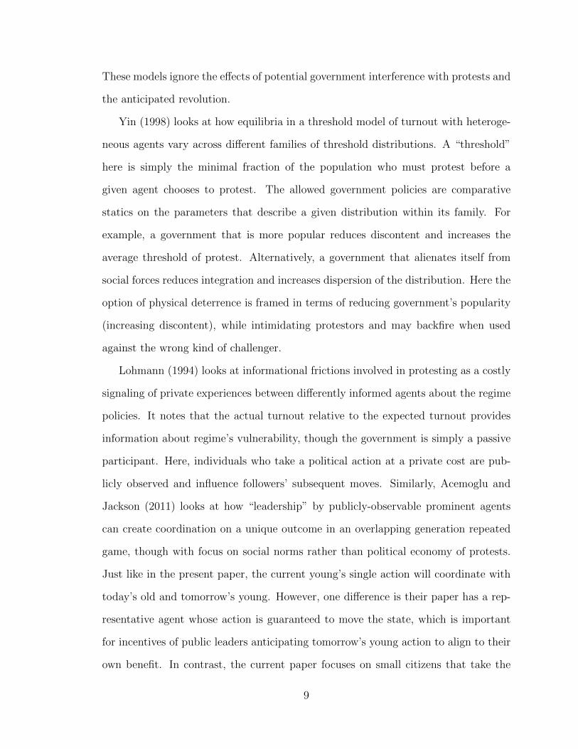
These models ignore the effects of potential government interference with protests and

the anticipated revolution.

Yin (1998) looks at how equilibria in a threshold model of turnout with heteroge-

neous agents vary across different families of threshold distributions. A “threshold”

here is simply the minimal fraction of the population who must protest before a

given agent chooses to protest. The allowed government policies are comparative

statics on the parameters that describe a given distribution within its family. For

example, a government that is more popular reduces discontent and increases the

average threshold of protest. Alternatively, a government that alienates itself from

social forces reduces integration and increases dispersion of the distribution. Here the

option of physical deterrence is framed in terms of reducing government’s popularity

(increasing discontent), while intimidating protestors and may backfire when used

against the wrong kind of challenger.

Lohmann (1994) looks at informational frictions involved in protesting as a costly

signaling of private experiences between differently informed agents about the regime

policies. It notes that the actual turnout relative to the expected turnout provides

information about regime’s vulnerability, though the government is simply a passive

participant. Here, individuals who take a political action at a private cost are pub-

licly observed and influence followers’ subsequent moves. Similarly, Acemoglu and

Jackson (2011) looks at how “leadership” by publicly-observable prominent agents

can create coordination on a unique outcome in an overlapping generation repeated

game, though with focus on social norms rather than political economy of protests.

Just like in the present paper, the current young’s single action will coordinate with

today’s old and tomorrow’s young. However, one difference is their paper has a rep-

resentative agent whose action is guaranteed to move the state, which is important

for incentives of public leaders anticipating tomorrow’s young action to align to their

own benefit. In contrast, the current paper focuses on small citizens that take the

9

sequence of states as given in any Markov Perfect Equilibrium, which generates ad-

ditional within-period multiplicity as agents can find it optimal to demand various

policing levels inside an interval as long as everyone else in the current period does

and deviates otherwise.

Another informational model by Edmond (2011) allows for a strategic government

to manipulate quality and quantity of information through propaganda. On one

hand, the innovation of centralized mass-media like newspapers and television makes

it easier for the government to stay in power, but on the other hand, the more

decentralized social networks make it more difficult to prevent protest through a

relative increase in informational reliability. This model emphasizes informational

rather than time frictions as it studies propaganda and signal filtering rather than

relationship between anticipation and dynamic evolution of play.

Like the present paper, Cho and Matsui (2005) also studies a repeated game of

asymmetric moves but focuses on the private sector (a single representative agent)

that coordinates with the government on inflation-setting and its expectation. The

private sector isn’t coordinating with itself, though - only with the government’s last

action and tomorrow’s action. The idea to use a time-varying fundamental to reduce

equilibrium multiplicity was used by Burdzy, Frankel, and Pauzner (2001). The

anticipation of future play with locked-in actions had them focus on a risk-dominant

outcome. The present paper introduces variation in small player payoffs through

equilibrium actions of a large strategic player, rather than exogenous shocks. Even

if the players’ own costs of work are fixed, they may still anticipate their endogenous

cost of protest to vary in the future because the large player’s incentives change.

This makes revolution happen sooner without completely pinning down its timing,

which would go against observers’ surprise at the collapse of the Berlin Wall as was

extensively documented by Kuran (1991).

10

The rest of the paper is structured as follows. Section 2.1 presents a simple

static model which will be the stage game in the subsequent dynamic framework.

Section 2.2 repeats the stage game in a dynamic model with a stationary police

productivity. Section 2.3 introduces a downward trend in police productivity and

Section 2.4 concludes. Finally, Appendix B contains some of the proofs from the

main text.

2.1 Simplified Model (one-shot)

Consider a static, one-period model that will highlight some of the flavor of later

results in a simpler setting. We will find that the government’s policing is non-

monotone in citizen’s cost of work for different equilibria. One limitation of the

static model is that it doesn’t capture the spontaneity and turbulence of revolution.

There are no interactions via expectations for adjacent states - in the static model

these belong to different equilibria. On the other hand, in the dynamic model with a

trend, knowing that the government will eventually fall can coordinate expectations

against it much sooner. Knowing that, the government may have to increase policing

before revolution to keep agitated citizens working. Such increase would push the

timing of the revolution closer to the present because with declining productivity, the

government wouldn’t be able to afford it in the future when it may have survived

with optimistic citizens.

While the static model doesn’t capture the dynamic interactions, the setup and

the solution of the stage game is illustrative of the steps taken to solve the repeated

game.

The government observes the fundamental state θ P r0,8q, which is publicly

known, and represents citizens’ cost of work2. Next, the government commits to a

policing level ppθq P r0,8q.

2In the later, more general model this will be denoted as fixed parameter B.

11

After observing that the government has already committed to some policing level

p and the fundamental is θ, measure 1 of citizens pick an action a P t0, 1u where a “ 0

represents “protest” or “joining the opposition” and a “ 1 represents “work.”

Focusing on the symmetric pure strategies, aggregate choice a P t0, 1u can be

thought of as the labor force. For simplicity of exposition we will focus on a subset

of symmetric, pure-strategy Subgame Perfect Equilibria where citizen’s strategy is a

cutoff pcθq.

aθppq “

$

’

’

&

’

’

%

1 if p ě cθ,

0 if p ă cθ,

(2.1.1)

Citizens prefer work relative to protest more when policing rises as they prefer to avoid

pain. They also work more when labor force rises because they prefer to conform or

because the cost of repression is higher for smaller crowd of remaining protestors.

Let the relative preference for work over leisure, given labor force aggregate L and

policing p, be denoted as

∆upL, p; θq “ up1, L, p; θq ´ up0, L, p; θq “ αL` p´Θ (2.1.2)

The parameter α is the measure of social cohesion (strategic complementarity), how

strong the preference for conformity is and θ is a cost of working (preference for

leisure).

Government’s payoff increases in the labor force (less unrest, more taxes - not

modeled) and decreases in the police force (police and justice department budgets

are costly).

gpL, pq “ L´1

γp : t0, 1u ˆ r0,8q Ñ R, (2.1.3)

12

where 1γ

is the marginal cost of policing and γ is a measure of policing productivity

which is high when policing cost is low.

A pair of strategies (cθ, p˚pθq) form a Subgame-Perfect Equilibrium when they

have no profitable deviations in every state. While the government faces state θ, the

citizens face state pθ, pq.

An individual citizen recognizes the equilibrium labor-force in state pθ, pq to be

L “ 1pěcθ . They find it optimal to work if and only if ∆upL, p; θq ě 0 which happens

if and only if

p ě θ ´ αL “ θ ´ α1pěcθ (2.1.4)

It can’t be the case that the citizen finds it optimal to protest for any policing level

(even out-of-equilibrium) above the cutoff strategy, p ě cθ as that would violate

Subgame-Perfection. Equation (2.1.4) becomes a restriction on the equilibrium cutoff

strategy:

cθ ě θ ´ α (2.1.5)

Similar considerations give another restriction to prevent citizen from deviating to

work when everyone protests in some state below the cutoff with p ă cθ :

cθ ď θ (2.1.6)

Combining equations (2.1.5) and (2.1.6), cθ satisfies collectively-sustained best-

response (BR) if and only if

cθ P rθ ´ α, θs (2.1.7)

As explained above, cθ ą θ violates equation (2.1.6) because if policing p satisfies

cθ ą p ą θ, then each citizen finds it optimal to work and deviates from equilibrium-

prescribed protest. Similarly, cθ ă θ´α violates equation (2.1.5) because if policing

13

p satisfies cθ ă p ă θ ´ α, then each citizen finds it optimal to protest and deviates

from equilibrium-prescribed work.

The government takes citizen’s cutoff strategy cθ as given. Thus, government’s

optimal choice maximizes:

gpL, pq “ L´1

γp (2.1.8)

The optimal policing level turns out to be either zero or equal to the citizen’s

cutoff cθ.

ppθq “ arg maxpt1pěcθ ´

1

γpu P t0, cθu (2.1.9)

Observe that ppθq “ cθ if and only if 1´ cθγě 0 if and only if cθ ď γ and, otherwise,

ppθq “ 0 if and only if cθ ą γ.

Thus,

ppθq “

$

’

’

&

’

’

%

cθ if cθ ď γ,

0 if cθ ą γ,

(2.1.10)

Assumption 2.1. : γ ą 2α, so social cohesion isn’t too great.

The purpose of this assumption is to ensure ppγq ą ppαq for the next proposition.

It also ensures ppθq ” 0 is not an equilibrium outcome for all θ ě 0. In particular, the

proof of the following proposition will establish that in every SPE, there has to be a

positive police level at θ “ γ2:

p˚pγ{2q “ cθ ě θ ´ α “γ

2´ α ą 0. (2.1.11)

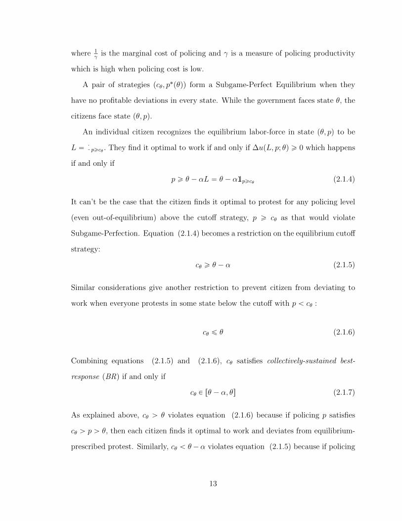
Proposition 2.2 (Non-Monotonicity). There exist costs of work θL ď θM ď θH : for

any equilibrium selection picking arbitrary SPE pp˚pθq, c˚θq for each state, the policing

14

Figure 2.1: One-shot game gives a preview of a dynamic resultp(θ)

α

Policing Non-Monotonicity

γ+αθp(θH) θL=γ/2 θM=

γ θH>γ+α

p(θL)

p(θM)

θ

θ-αγ

γ+α

in these states is non-monotone and satisfies

p˚pθHq ă p˚pθLq ă p˚pθMq

Proof. See Appendix.

For every cost of work θ, a Subgame-Perfect Equilibrium pp˚pθq, c˚θq has Never

Revolt at θ when the equilibrium labor supply is 1 (full employment, no protests)

because p˚pθq “ cθ. Likewise, a Subgame-Perfect Equilibrium has Never Revolt at θ

when the equilibrium labor supply is 0 (no employment, everyone protests) because

p˚pθq “ 0 ă cθ.

Proposition 2.3. 1. If 0 ď θ ď γ, then all equilibria have Never Revolt (NR) at

θ and policing satisfies

θ ´ α ď p˚pθq “ c˚θ ď θ

2. If θ ą γ ` α, then all equilibria have Always Revolt (AR) at θ and policing

satisfies

p˚pθq “ 0 ă θ ´ α ď c˚θ ď θ

15

3. If γ ă θ ď γ`α, then both NR and AR are attained in different equilibria at θ.

Proof. See Appendix.

The main idea of Proposition 2.2 will be recreated for the dynamic case in Theorem

2.31. They both say that when the government police is productive relative to the

cost of work it enforces, then there is a moderate amount of policing. As the cost of

work rises in Proposition 2.2, while keeping police productivity fixed (alternatively:

as the government police gets less productive in Theorem 2.31, while cost of work is

fixed), policing first increases and at some point when policing is so unproductive it’s

useless, then policing stops completely (abruptly, rather than smoothly). While the

basic results are similar, the mechanism is different. In the one-shot model, cost of

work increases exogenously and continuously, so slightly more policing today keeps

the citizens indifferent between work and protest at their threshold cutoff. On the

other hand, in the dynamic case what’s changing is that on the period before the

revolution begins (i) the tomorrow’s old protest which discourages work today, (ii)

continuation utility of receiving policing tomorrow becomes zero since the government

gives up, also reducing payoff to work. These two factors cause a discontinuous drop

in relative utility of work, so today’s policing needs to be higher by a “jump” to

compensate.

The same two factors also have a qualitative effect on the equilibrium set. Taking

the dynamic model with the stationary states as a baseline and then adding cas-

cading endogenous anticipation resolves multiplicity for some states adjacent to the

dominance region. For example, in the stationary region with low-moderate police

productivity it is possible to sustain multiple equilibria (at least Traditional Play

and Always Revolt) that rely on self-fulfilling beliefs about the future coordination

(Proposition 2.18). Once we introduce anticipation of eventual and certain (no matter

how far in the future) deterioration of police productivity, today’s equilibrium path

16

gets uniquely resolved into Always Revolt by contagion of dominance (Proposition

2.29).

2.2 Fundamentals of the Repeated Game

This section is going to make the first step towards a dynamic version of the one-shot

model - the citizens will live for two periods, not only playing a coordination game

with today’s young but also with today’s old (yesterday’s young) and tomorrow’s

young (when they’re themselves old). Secondly, the government’s policing problem

has a substitution trade-off between tomorrow’s policing and today’s policing, though

Markov Perfection will be used to pin down tomorrow’s equilibrium choice, so time

inconsistency problem doesn’t arise directly3.

The government is a long-lived player with 0 ă δ ă 1 discount and citizens are

short-lived, assumed to live for two periods with 0 ă β ă 1 discount. There is a

measure 12

of citizens that are born every period and commit to an action a P t0, 1u

for both periods, where a “ 0 represents “protest” or “joining the opposition” and

a “ 1 represents “work.” Citizens are “Young” when they are born and decide their

action and are “Old” when they are stuck playing what they chose last period.

At the beginning of period t, the government observes the average action of the

Old ao before picking a policing level pt P r0,8q. Focusing on the symmetric pure

strategies, ao P t0, 1u. Then the Young are born and they observe both pao, ptq before

picking work or protest a P t0, 1u. The labor force is the total amount of work done

3Time-consistency is achieved through matching particular cutoffs. When the government is lesspatient than the citizens, then among all NR equilibria with full employment, the most preferredequilibrium has the government commit to “maximum” (in a certain sense) policing tomorrow andevery other period after by having maximum (pessimistic) citizen’s cutoff, as if government wasgiving up its bargaining power

17

by the Old and the Young combined,

Lt “ p1{2qao` p1{2qay. (2.2.1)

The labor force is restricted to t0, 12, 1u for symmetric equilibria in pure strategies.

Government’s Markov strategy in state a, the Old’s average work level, is the

policing level:

ppaq : t0, 1u Ñ r0,8q (2.2.2)

(Young) citizen’s Markov strategy in state pa, pq, which is the Old’s work level

and government policing level, is the choice between protest and work:

apa, pq : t0, 1u ˆ r0,8q Ñ t0, 1u (2.2.3)

For simplicity of exposition we will focus on a subset of symmetric, pure-strategy

Markov Perfect Equilibria where citizen’s strategy is a cutoff pc0, c1q.4 Citizen works

when policing in state a P t0, 1u exceeds ca and protests otherwise.

apa, pq “

$

’

’

&

’

’

%

1 if p ě ca,

0 if p ă ca,

(2.2.4)

At the end of period t, payoffs are realized based on pL, pq, which is current labor and

policing. Citizens prefer work relative to protest more when policing rises as they

prefer to avoid pain. They also work more when labor force rises because they prefer

to conform or because the cost of repression is higher for smaller crowd of remaining

4For each cutoff c´strategy, there is a family Spcq of strategies that are the same for p P r0, casbut possibly equal to 0 on an open set p P pca, ca ` εq for some ε and equal to 1 for greater p.The behavior above ca relies on out-of-equilibrium calculation but may be consistent because ofcoordination. Using c P Spcq doesn’t change the results because of Lemma 2.10.

18

protestors. Government’s payoff increases in the labor force (less unrest, more taxes -

not modeled) and decreases in the police force (police and justice department budgets

are costly).

For simplicity of exposition, government’s one-period payoff is assumed to be linear

in labor and policing:

gpL, pq “ L´1

2γp : t0,

1

2, 1u ˆ r0,8q Ñ R, (2.2.5)

where 12γ

is marginal cost of policing and γ is a measure of policing productivity which

is high when policing cost is low.

Government is a long-lived agent and receives normalized discounted total payoff

of

p1´ δq8ÿ

t“0

δtpLt ´1

2γptq (2.2.6)

Citizen’s one-period payoff for choosing a, when total labor force is L and policing

is p, is denoted by

upa, L, pq : t0, 1u ˆ t0,1

2, 1u ˆ r0,8q Ñ R. (2.2.7)

Citizen born at t receives total utility for playing at as their current one-period

payoff plus discounted tomorrow’s payoff for playing at as well:

upat, Lt, ptq ` βupat, Lt`1, pt`1q (2.2.8)

Next, we will impose a linearity assumption on citizen’s payoffs as follows. Let the

relative preference for work over leisure within one period, given pL, pq, be denoted

19

as

∆upL, pq “ up1, L, pq ´ up0, L, pq “ αL` p´B (2.2.9)

where α,B are parameters. α is the measure of social cohesion (strategic comple-

mentarity), how strong the preference for conformity is and B is a cost of working

(preference for leisure).

Assumption 2.4. 0 ă α ă B. The cost of work exceeds gains from complete coordi-

nation on work without policing (unpopular dictator).5

We can make the following simple observations by using linear functional forms

for flow preferences of citizens and the government.

Observation 2.5. ∆upL, pq “ αL ` p ´ B. It is monotonically increasing in L

(preference for conformity).

Observation 2.6. ∆upL, pq “ αL`p´B is monotonically increasing in p (preference

for avoiding pain).

Observation 2.7. gpL, pq “ L ´ 12γp is monotonically increasing in L (government

is more popular, country more productive).

Observation 2.8. gpL, p “qL´ 12γp is monotonically decreasing in p (costly budgets).

2.2.1 Markov Perfect Equilibrium conditions

The solution concept used is Markov Perfect Equilibrium in pure strategies. A pair

of Markov strategies (a˚, p˚) are MPE when they withstand one-shot deviation in

every state. Optimality on off-equilibrium path will be relevant for citizen’s cutoff

choice. Citizens consider facing arbitrary policing levels to which the government has

5This assumption will be discussed in greater detail in Section 2.2.2.

20

previously committed to on its turn, not simply specific equilibrium quantity pp˚0 , p˚1q

and ensuring the citizen does indeed protest in all states below the cutoff and works

for all states above the cutoff.

The government moves first and its policing function, ppaq, depends only on the

observed old’s action, a. p˚paq : t0, 1u Ñ r0,8q. The young citizen moves after

observing government’s choice as well as the old’s action and its cutoff strategy is

a˚pa, pq “ 1tpěc˚a u : t0, 1u ˆ r0,8q Ñ t0, 1u Government receives utility from p˚ at

state a, taking the citizen cutoff strategy pc0, c1q as given, as follows

Gpa|p˚q “ p1´ δq

ˆ

a

2`1tp˚aěcau

2´

1

2γp˚a

˙

` δGp1tp˚ěcau|p˚q (2.2.10)

Denote government utility from one-shot deviation to p P r0,8q and later going

back to p˚ as

Gpa|p˚q “ p1´ δq

ˆ

a

2`1tpěcau

2´

1

2γp

˙

` δGp1tpěcau|p˚q (2.2.11)

Taking (a˚) as given, government’s choice p˚a is optimal for every a P t0, 1u:@p P

r0,8q :

p1´ δqg pL˚, p˚aq ` δG`

1tp˚aěcau|p˚˘

ě p1´ δqg´

L, p¯

` δG`

1tpěcau|p˚˘

(2.2.12)

Expanding the payoff functions and simplifying, the government does not benefit in

any state a P t0, 1u from a one-shot deviation today to p from p˚ :

p1´ δq

ˆ

1tp˚aěcau

2´p˚a2γ

˙

` δG`

1tp˚aěcau|p˚˘

ě p1´ δq

ˆ

1tpěcau

2´

p

2γ

˙

` δG`

1tpěcau|p˚˘

(2.2.13)

21

Citizens are “small” players, who individually cannot move tomorrow’s state, which

is the next period’s Old labor contribution. They are followers in a Stackelberg

repeated subgame where the government leads with some pa. Therefore, there is an

aggregate best-response strategy that is played, so that citizens don’t have incentive

to unilaterally deviate from it.

Suppose that in state pa, pq a young citizen will face p policing today and p1

policing tomorrow as well as L labor force today and L1 labor force tomorrow. The

difference in a young citizen’s total utility from choosing to work instead of protest

today is the following:

∆U “ pup1, L, pq ` βup1, L1, p1qq ´ pup0, L, pq ` βup0, L1, p1qq

“ ∆upL, pq ` β∆upL1, p1q (2.2.14)

Note that the young citizen’s unilateral choice doesn’t affect the state, the transition

path of the labor force or the policing levels in either period. The citizen works when

∆upL, pq ` β∆upL1, p1q ě 0 (2.2.15)

and the citizen protests when

∆upL, pq ` β∆upL1, p1q ă 0. (2.2.16)

Next we will state conditions on other citizen’s c˚´strategy cutoff for MPE. In

each state pa, pq and taking government strategy p as given, each citizen playing

1tpaěc˚a u

needs to be a best-response to other citizens playing the same c˚´strategy

both periods and government playing p next period.6

6At the time of Young citizen’s move, the observed p today is already fixed and need not derivefrom p as MPE conditions require optimality in all states.

22

Suppose we are in state pa, pq with other citizens following c˚-strategy prescribing

work (c˚a ď p) and government following p-strategy. An individual citizen also prefers

to work over protest if:

∆U “ ∆u

ˆ

a

2`

1

2, p

˙

` β∆u

ˆ

1

2`

1

21tp1ěc

˚1 u, p1

˙

ě 0 (2.2.17)

Expanding the payoff functions, noting today’s young and tomorrow’s old work and

simplifying, we get:

@a P t0, 1u, @p ě c˚a : p ě p1` βqB ´ α

ˆ

1` β

2`a

2`β1tp1ěc˚1 u

2

˙

´ βp1 (2.2.18)

The above condition on work, a “ 1, to be a collectively sustained citizen best-

response holds for all p ě c˚a if and only if

@a P t0, 1u, c˚a ě p1` βqB ´ α

ˆ

1` β

2`a

2`β1tp1ěc˚1 u

2

˙

´ βp1 (2.2.19)

To describe (2.2.19) condition, define the following auxiliary function:

ppp1, a, a1q ” p1` βqB ´ α

ˆ

1` β

2`a` a1β

2

˙

´ βp1 (2.2.20)

In each state a P t0, 1u, if others use c˚a and government uses p˚a, it is optimal to work

@p ě c˚a :

@a P t0, 1u, c˚a ě ppp1, a,1tp1ěc˚1 uq (2.2.21)

Suppose in state pa, pq with other citizens following c˚-strategy prescribing protest

(c˚a ą p) and government follows p-strategy. An individual citizen also prefers to

23

protest over work if:

@a P t0, 1u, @p ă c˚a,∆U “ ∆u´a

2, p¯

` β∆u

ˆ

1

21tp0ěc

˚0 u, p0

˙

ă 0 (2.2.22)

Simplifying, noting today’s young protest and so tomorrow’s old protest, we get:

@a P t0, 1u, @p ă c˚a : α

ˆ

a

2`β1tp0ěc˚0 u

2

˙

` p` βp0 ă p1` βqB (2.2.23)

The above condition on protest being a collectively sustained best-response holds if

and only if

@a P t0, 1u, c˚a ď p1` βqB ´ βp0 ´ α

ˆ

a

2`β1tp0ěc˚0 u

2

˙

(2.2.24)

To describe (2.2.24) condition, define the following auxiliary function:

ppp0, a, a0q ” p1` βqB ´ βp0 ´ α

ˆ

a` a0β

2

˙

(2.2.25)

In each state a P t0, 1u, if others use c˚a and government uses p˚a, it is optimal to

protest @p ă c˚a :

@a P t0, 1u, c˚a ď ppp0, a,1tp0ěc˚0 uq (2.2.26)

Compare the α coefficient on the RHS of (2.2.19) when young citizens coordinate

on work and RHS of (2.2.24) when young citizens coordinate on protest. In the

former case, citizen derives coordination utility of 12

from working alongside with

1{2 population of the young today and β2

from working with 1{2 population of the

old tomorrow. In the later case, today’s young and tomorrow’s old protest instead

because p ă c˚a.

24

2.2.2 Characterizing Government’s Best Response

Assumption 2.9. Police productivity γ is constant over time.

For the purposes of generating benchmark equilibrium sets in Section 2.2, Assump-

tion 2.9 fixes γ within the scope of each game. In each case, each equilibrium set is

parametrized by γ. In contrast, Section 2.3 will relax this assumption and let γ vary

over time, focusing on decreasing police productivity.7 One important implication is

that under constant γ, time t is not a payoff-relevant state variable for the purposes of

MPE in Section 2.2. However, observing a publicly known and anticipated sequence

γt makes time t a payoff-relevant state variable in Section 2.3.

When the old play a, citizen strategy a˚pa, pq “ 1tpěc˚a u assigns work or leisure

for each p. Markov perfection requires optimality for all p, even those not reached

in equilibrium. This consistency requires that no one has the incentive to deviate

against the prescribed action, a˚pa, pq. For very large values of p, ∆u is large and

eventually individual incentives to work override preference for cohesion. Therefore,

for every equilibrium, a˚pa, pq “ 1 for p sufficiently large. In this case, today’s young

prefer to work even if there is no policing tomorrow. This means it is always feasible

for the government to enforce work by policing high enough, though not necessarily

always optimal.

The following argument establishes this upper-dominance region using Eq.

(2.2.26) by putting an upper bound on citizen’s cutoff used in any MPE. When

p ą p1 ` βqB citizen’s best-response is always work because policing today is high

enough to cover cost of work for both periods even if everyone else protests and any

additional coordination is a bonus. Recall that

ppp0, a, a0q “ p1` βqB ´ βp0 ´ α

ˆ

a` a0β

2

˙

(2.2.27)

7It is known that policing will be less effective in the future, perhaps because of military andlaw-enforcement beginning to sympathize with the opposition.

25

and note it is monotonically decreasing in all arguments because some policing today

can be substituted by policing tomorrow or coordination with other citizens.

Fix any MPE tpp˚0 , p˚1q, pc

˚0 , c

˚1qu and apply (2.2.26):

@a P t0, 1u, c˚a ď ppp˚0 , a,1tp˚0ěc˚0 uq ď ppp˚0 , 0, 0q “ p1` βqB ´ βp˚0 ď p1` βqB

(2.2.28)

The second inequality from monotonicity. Similarly, a˚pa, pq “ 0 for sufficiently

small p if government’s strategy were to prescribe small policing in the good state

tomorrow that is reached when today’s young pick work.

We now establish there is a similar lower-dominance region where very low policing

today makes protest dominant. This means government will face definite protests if it

never polices. If tomorrow’s policing is not too great, so that today’s policing choice

is meaningful p˚1 ă1`ββpB ´ αq, then @a P t0, 1u : c˚a ą 0. 8. To see this, recall that

ppp1, a, a1q “ p1`βqB´βp1´α`

1`β2`

a`a1β2

˘

and note it is monotonically decreasing

in all arguments.

Fix any MPE tpp˚0 , p˚1q, pc

˚0 , c

˚1qu that satisfies p˚1 ă

1`ββpB´αq and apply (2.2.21):

@a P t0, 1u, c˚a ě ppp˚1 , a,1tp˚1ěc˚a uq ě ppp˚1 , 1, 1q “ p1` βqpB ´ αq ´ βp˚1 ą 0 (2.2.29)

The second inequality from monotonicity. Then c˚a ą 0 and citizen’s best-response

is always protest when facing p P r0, c˚aq because the level of policing today and

tomorrow are not enough to cover the cost of work for both periods even if everyone

else works. Recall that Assumption 2.4 stated 0 ă α ă B and note that it is sufficient

to generate this lower-dominance region. Its economic interpretation is that citizens

work only when government sufficiently polices enough and, in particular, never work

8Here p˚1 ě 0 is well defined because B ą α by Assumption 2.4

26

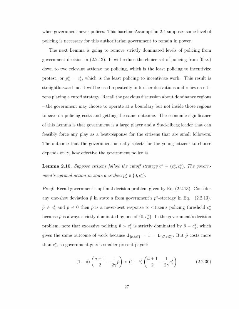
when government never polices. This baseline Assumption 2.4 supposes some level of

policing is necessary for this authoritarian government to remain in power.

The next Lemma is going to remove strictly dominated levels of policing from

government decision in (2.2.13). It will reduce the choice set of policing from r0,8q

down to two relevant actions: no policing, which is the least policing to incentivize

protest, or p˚a “ c˚a, which is the least policing to incentivize work. This result is

straightforward but it will be used repeatedly in further derivations and relies on citi-

zens playing a cutoff strategy. Recall the previous discussion about dominance regions

– the government may choose to operate at a boundary but not inside those regions

to save on policing costs and getting the same outcome. The economic significance

of this Lemma is that government is a large player and a Stackelberg leader that can

feasibly force any play as a best-response for the citizens that are small followers.

The outcome that the government actually selects for the young citizens to choose

depends on γ, how effective the government police is.

Lemma 2.10. Suppose citizens follow the cutoff strategy c˚ “ pc˚0 , c˚1q. The govern-

ment’s optimal action in state a is then p˚a P t0, c˚au.

Proof. Recall government’s optimal decision problem given by Eq. (2.2.13). Consider

any one-shot deviation p in state a from government’s p˚-strategy in Eq. (2.2.13).

p ‰ c˚a and p ‰ 0 then p is a never-best response to citizen’s policing threshold c˚a

because p is always strictly dominated by one of t0, c˚au. In the government’s decision

problem, note that excessive policing p ą c˚a is strictly dominated by p “ c˚a, which

gives the same outcome of work because 1tpěc˚a u “ 1 “ 1tc˚aěc˚a u. But p costs more

than c˚a, so government gets a smaller present payoff:

p1´ δq

ˆ

a` 1

2´

1

2γp

˙

ă p1´ δq

ˆ

a` 1

2´

1

2γc˚a

˙

(2.2.30)

27

Of course, the continuation values are the same, Gp1|p˚q, because tomorrow’s state

a “ 1 in both cases.

p1´ δq

ˆ

1

2´

1

2γc˚a

˙

` δG p1|p˚q ą p1´ δq

ˆ

1

2´

1

2γp

˙

` δG p1|p˚q (2.2.31)

Similar argument eliminates any positive policing that is strictly below the cutoff,

0 ă ppaq ă c˚a, because such policing is strictly dominated by 0 where tomorrow’s

state is 0 in both cases but is cheaper to achieve with no policing than below-threshold

positive policing:

p1´ δq p0q ` δG p0|p˚q ą p1´ δq

ˆ

´1

2γpq

˙

` δG p0|p˚q (2.2.32)

This means, the best-response for the government at state a is always in t0, c˚au,

which simplifies government’s decision problem into binary choice.

Next, we consider government’s best-response to some given pc0, c1q citizen strat-

egy, resilient to one-shot deviation from Eq. (2.2.13). There are four possible govern-

ment best-responses (two possible actions in each of two states).

Categorize government’s continuation strategy by the unique labor paths it in-

duces:

• “Always Revolt” (AR) if p˚0 “ p˚1 “ 0. Young and old both protest.

• History-dependent “Traditional Play” (TR) if p˚0 “ 0, p˚1 “ c˚1 . Young and old

play the same.

• “Counter-Culture” (CC) if p˚0 “ c˚0 , p˚1 “ 0. Young play the oppoite of old.

28

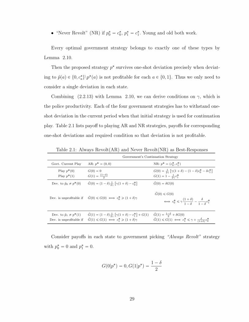
• “Never Revolt” (NR) if p˚0 “ c˚0 , p˚1 “ c˚1 . Young and old both work.

Every optimal government strategy belongs to exactly one of these types by

Lemma 2.10.

Then the proposed strategy p˚ survives one-shot deviation precisely when deviat-

ing to ppaq P t0, c˚auzp˚paq is not profitable for each a P t0, 1u. Thus we only need to

consider a single deviation in each state.

Combining (2.2.13) with Lemma 2.10, we can derive conditions on γ, which is

the police productivity. Each of the four government strategies has to withstand one-

shot deviation in the current period when that initial strategy is used for continuation

play. Table 2.1 lists payoff to playing AR and NR strategies, payoffs for corresponding

one-shot deviations and required condition so that deviation is not profitable.

Table 2.1: Always Revolt(AR) and Never Revolt(NR) as Best-Responses

Government’s Continuation Strategy

Govt. Current Play AR: p˚ “ p0, 0q NR: p˚ “ pc˚0 , c˚1 q

Play p˚p0q Gp0q “ 0 Gp0q “ 12γ

“

γp1` δq ´ p1´ δqc˚0 ´ δc˚1

‰

Play p˚p1q Gp1q “ p1´δq2

Gp1q “ 1´ 12γc˚1

Dev. to p0 ‰ p˚p0q Gp0q “ p1´ δq 12γ

“

γp1` δq ´ c˚0‰

Gp0q “ δGp0q

Dev. is unprofitable if Gp0q ď Gp0q ðñ c˚0 ě p1` δqγGp0q ď Gp0q

ðñ c˚0 ď γp1` δq

1´ δ´

δ

1´ δc˚1

Dev. to p1 ‰ p˚p1q Gp1q “ p1´ δq 12γ

“

γp1` δq ´ c˚1‰

`Gp1q Gp1q “ 1´δ2` δGp0q

Dev. is unprofitable if Gp1q ď Gp1q ðñ c˚1 ě p1` δqγ Gp1q ď Gp1q ðñ c˚1 ď γ ` δp1`δq

c˚0

Consider payoffs in each state to government picking “Always Revolt” strategy

with p˚0 “ 0 and p˚1 “ 0.

Gp0|p˚q “ 0, Gp1|p˚q “1´ δ

2

29

In state a “ 0, the relevant deviation to consider by Lemma 2.10 is p0 “ c˚0 that

forces today’s young to work and then reverting to p˚ “ p0, 0q next period, so that

all future young protest as before. The corresponding payoff is:

Gp0|p˚q “p1´ δq

ˆ

1

2´

1

2γc˚0

˙

` δp1´ δq

2

“ p1´ δq

„

p1` δq

2´

1

2γc˚0

“ p1´ δq1

2γrγp1` δq ´ c˚0s (2.2.33)

The initial strategy induces protest in every period. Under the deviation, only the

first two periods differ in outcomes: after observing today’s old protesting, the young

work today and tomorrow’s old work but tomorrow’s young protest just like under

“AR.” The deviation is not profitable, if policing today with cost 12γc˚0 that exceeds

the benefit from today’s young working for two periods p1`δq2.

0 “ Gp0|p˚q ě Gp0|p˚q ðñ c˚0 ě γp1` δq (2.2.34)

In state a “ 1, the relevant deviation to consider by Lemma 2.10 is p1 “ c˚1 that

forces today’s young to work and then reverting to p˚ “ p0, 0q next period, so that

all future young protest as before. The corresponding payoff is:

Gp1|p˚q “p1´ δq

ˆ

1` 1

2´

1

2γc˚1

˙

` δp1´ δq

2

“ p1´ δq1

2γrγp1` δq ´ c˚1s `

1´ δ

2(2.2.35)

Under the deviation, only the first two periods differ in outcomes: after observing

today’s old working, the young work today and tomorrow’s old work but tomorrow’s

young protest just like under “AR.” The deviation is not profitable, if policing today

30

with cost 12γc˚1 that exceeds the benefit from today’s young working for two periods

p1`δq2.

Gp1|p˚q ě Gp1|p˚q

ðñ1´ δ

2ě p1´ δq

1

2γrγp1` δq ´ c˚1s `

1´ δ

2

ðñ c˚1 ě γp1` δq (2.2.36)

Consider payoffs in each state to government picking the “Never Revolt” strategy

p˚0 “ c˚0 , p˚1 “ c˚1 .

When the old work, the government’s payoff along the equilibrium path, after

inducing today’s young to work, is

Gp1|p˚q “ p1´ δqp1´1

2γc˚1q ` δGp1|p

˚q “ 1´

1

2γc˚1 , (2.2.37)

When the old protest, the government’s payoff along the equilibrium path, after

inducing today’s young to work, is

Gp0|p˚q “ p1´ δq

ˆ

1

2´

1

2γc˚0

˙

` δGp1|p˚q

“1` δ

2´ p1´ δq

1

2γc˚0 ´ δ

1

2γc˚1

“1

2γpγp1` δq ´ p1´ δqp˚0 ´ δc

˚1q (2.2.38)

In state a “ 0, the relevant deviation to consider by Lemma 2.10 is pp0q “ 0 that

allows today’s young to protest and then reverting to p˚ “ pc˚0 , c˚1q next period, so

that all future young work as before. The corresponding payoff is smaller if:

31

Gp0|p˚q “ 0` δGp0|p˚q, Gp0|p˚q ě Gp0|p˚q ðñ Gp0|p˚q ě 0

ðñ γp1` δq ´ p1´ δqp˚0 ´ δc˚1 ě 0

ðñp1` δq

2ě p1´ δq

1

2γp˚0 `

1

2γδc˚1 (2.2.39)

Here the requirement is that policing required at a “ 0 is low enough:

c˚0 ď γp1` δq

1´ δ´

δ

1´ δc˚1 (2.2.40)

Under the prescribed strategy, it is cheaper to pay p˚0 today and p˚1 tomorrow for

total cost of 12γpp˚0 ` δp˚1q and get benefit 1`δ

2of today’s young working than pay p˚0

tomorrow for total cost of δ 12γp˚0 and get no benefit. The net cost of adhering to the

strategy is 12γp1 ´ δqp˚0 ` δp˚1 is smaller than the net gain p1`δq

2. Deviation for state

a “ 1 can be evaluated similarly.

Table 2.2 is analogous for CC and TR strategies.

Table 2.2: Counter Culture(CC) and Traditional Play(TR) as Best-Responses

Government’s Continuation Strategy

Government’s Current Play CC: p˚ “ pc˚0 , 0q TR: p˚ “ p0, c˚1 q

Play p˚p0q Gp0q “12γ

1`δ

“

γp1` δq ´ c˚0‰

Gp0q “ 0

Play p˚p1q Gp1q “12γ

1`δ

“

p1` δqγ ´ δc˚0‰

Gp1q “ 1´ 12γc˚1

Dev. to p0 ‰ p˚p0q Gp0q “ δGp0q Gp0q “ 12γ

“

γp1` δq ´ p1´ δqc˚0 ´ δc˚1

‰

Dev. is unprofitable if Gp0q ď Gp0q ðñ c˚0 ď p1` δqγ Gp0q ď Gp0q ðñ c˚0 ě γ p1`δq1´δ

´ δ1´δ

c˚1

Dev. to p1 ‰ p˚p1q Gp1q “ p1´ δqp1´ 12γc˚1 q ` δGp1q Gp1q “ p1´δq

2

Dev. is unprofitable if Gp1q ď Gp1q ðñ c˚1 ě γ ` δp1`δq

c˚0 Gp1q ď Gp1q ðñ c˚1 ď γp1` δq

The following Proposition summarizes the results in the tables above.

Proposition 2.11. Suppose citizens are playing a cutoff strategy c˚ “ pc˚0 , c˚1q. The

government’s best-response p˚ is then unique a.e. (except when equality holds)

1. If c˚0 ě p1` δqγ and c˚1 ě p1` δqγ then the Best-Response is AR: p˚ “ p0, 0q

32

2. If c˚0 ď γ p1`δq1´δ

´ δ1´δ

c˚1 and c˚1 ď γ ` δp1`δq

c˚0 then the Best-Response is NR:

p˚ “ pc˚0 , c˚1q

3. If c˚0 ď p1` δqγ and c˚1 ě γ` δp1`δq

c˚0 then the Best-Response is CC: p˚ “ pc˚0 , 0q

4. If c˚0 ě γ p1`δq1´δ

´ δ1´δ

c˚1 and c˚1 ď γp1 ` δq, then the Best-Response is TR: p˚ “

p0, c˚1q

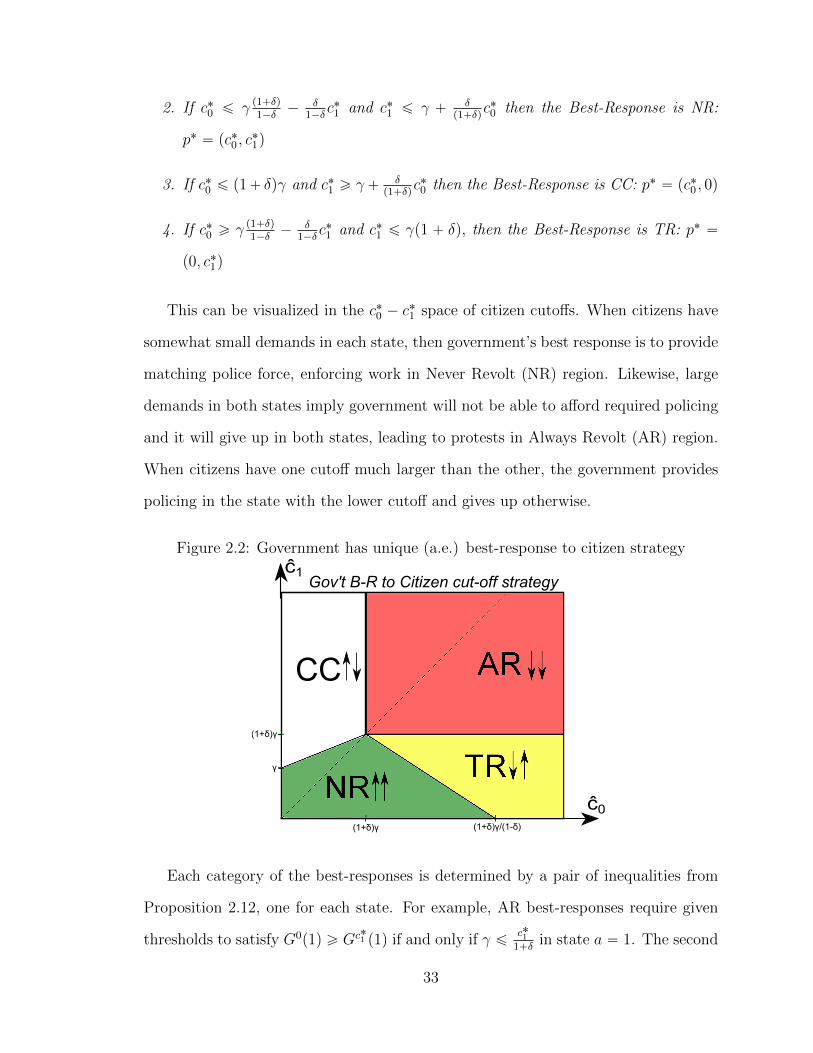
This can be visualized in the c˚0 ´ c˚1 space of citizen cutoffs. When citizens have

somewhat small demands in each state, then government’s best response is to provide

matching police force, enforcing work in Never Revolt (NR) region. Likewise, large

demands in both states imply government will not be able to afford required policing

and it will give up in both states, leading to protests in Always Revolt (AR) region.

When citizens have one cutoff much larger than the other, the government provides

policing in the state with the lower cutoff and gives up otherwise.

Figure 2.2: Government has unique (a.e.) best-response to citizen strategy

(1+δ)γ

(1+δ)γ/(1-δ)(1+δ)γ

γ

ĉ1Gov't B-R to Citizen cut-off strategy

ĉ0

CC

Each category of the best-responses is determined by a pair of inequalities from

Proposition 2.12, one for each state. For example, AR best-responses require given

thresholds to satisfy G0p1q ě Gc˚1 p1q if and only if γ ďc˚1

1`δin state a “ 1. The second

33

inqeuality they need to satisfy is 0 ě Gc˚0 p0q if and only if γ ďc˚0

1`δin state a “ 1,

which is a square region in the upper right of c˚0 ´ c˚1 plane.

2.2.3 Characterizing Citizen’s Best-Response Cutoff

Eq. (2.2.21) requires that facing high policing p in state a, p ě c˚a, young citizens

find it individually optimal to work, assuming other young conform to the equilib-

rium strategy cutoff c˚ “ pc˚0 , c˚1q and work. Secondly, Eq. (2.2.26) requires that

facing low policing p in state a, p ă c˚a, young citizens find it individually optimal to

protest, assuming other young conform to the equilibrium strategy cutoff c˚ “ pc˚0 , c˚1q

and protest. To be a best-response, a citizen’s strategy thus needs to satisfy both

conditions (2.2.21) and (2.2.26).

BRpp0, p1q “ tpc0, c1q : (2.2.21) and (2.2.26) are satisfiedu (2.2.41)

pc0, c1q P BRpp0, p1q means that, in all states, pc0, c1q is a best-response for indi-

vidual citizen to government playing p´strategy and other citizens playing the same

cutoff strategy pc0, c1q. BR is thus the set of all cutoffs that are best-responses to the

given government strategy and itself.

Proceed in three steps (see Appendix for details). First, Lemmas A.1 and A.2

characterize sets of cutoffs pc˚0 , c˚1q that satisfy each of the conditions – Equations

(2.2.21) and (2.2.26) respectively. These Lemmas A.1 and A.2 allow for government

to play arbitrary p˚. Secondly, by Lemma 2.10, government’s best-response is either

no policing or matching citizens’ cutoff. Using that, Lemma A.3 shows the results

from Lemmas 2.2 and 2.3 that are simplified for the special case when Government

plays zero policing or matches minimum policing. Thirdly, in Proposition 2.12, the

34

BR set, which is contained in the c0 ´ c1 space, is characterized by an intersection of

two intervals for each of the four relevant9 government plays.

Observe that by monotonicity of p in its third argument, a1, which is the action

of the young tomorrow after observing tomorrow’s old working:

ppp˚1 , 1, 1q ă ppp˚1 , 1, 0q. (2.2.42)

proposition combines previous two Lemmas to show that when government plays

one of tNR,AR, TR,CCu citizens’ BRpp˚0 , p˚1q is an interval where the lower bound

comes from Lemma 3.2.1 (no policing at a “ 1, p˚1 “ 0) or Lemma 3.4.1 (matching

policing at a “ 1, p˚1 “ c˚1) and the upper bound comes from Lemma 3.3.1 (no policing

at a “ 0, p˚0 “ 0 or Lemma 3.4.1 (matching policing at a “ 0, p˚0 “ c˚0). In all cases,

the best-response in state a to one of these four government candidate strategies is

proven to be an interval and can be succinctly expressed as

@a P t0, 1u, c˚a P rppp˚1 , a,1tp˚1ěc˚1 uq, ppp

˚0 , a,1tp˚0ěc˚0 uqs (2.2.43)

Proposition 2.12. Suppose pp˚0 , p˚1q is a given government strategy and pc˚0 , c

˚1q is a

citizen cutoff strategy.

1. Never Revolt (NR): If pp˚0 “ c˚0 , p˚1 “ c˚1q then pc˚0 , c

˚1q satisfies BRpp˚0 , p

˚1q if and

only if ppp˚1 , a, 1q ď c˚a ď ppp˚0 , a, 1q, for a “ 0, 1.

2. Always Revolt (AR): If pp˚0 “ 0, p˚1 “ 0q then c˚0 then pc˚0 , c˚1q satisfies BRpp˚0 , p

˚1q

if and only if ppp˚1 , a, 0q ď c˚a ď ppp˚0 , a, 0q, for a “ 0, 1.

3. Traditional Play (TR): If pp˚0 “ 0, p˚1 “ c˚1q then pc˚0 , c˚1q satisfies BRpp˚0 , p

˚1q if

and only if ppp˚1 , a, 1q ď c˚a ď ppp˚0 , a, 0q, for a “ 0, 1.

9In the sense that these plays are the only government best-responses to an arbitrary citizenstrategy.

35

4. Counter-culture (CC): If pp˚0 “ c˚0 , p˚1 “ 0q then pc˚0 , c

˚1q satisfies BRpp˚0 , p

˚1q if

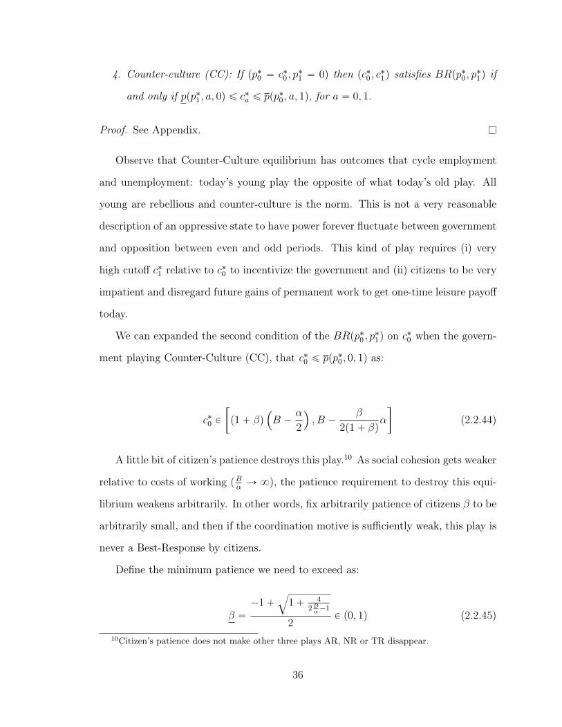
and only if ppp˚1 , a, 0q ď c˚a ď ppp˚0 , a, 1q, for a “ 0, 1.

Proof. See Appendix.

Observe that Counter-Culture equilibrium has outcomes that cycle employment

and unemployment: today’s young play the opposite of what today’s old play. All

young are rebellious and counter-culture is the norm. This is not a very reasonable

description of an oppressive state to have power forever fluctuate between government

and opposition between even and odd periods. This kind of play requires (i) very

high cutoff c˚1 relative to c˚0 to incentivize the government and (ii) citizens to be very

impatient and disregard future gains of permanent work to get one-time leisure payoff

today.

We can expanded the second condition of the BRpp˚0 , p˚1q on c˚0 when the govern-

ment playing Counter-Culture (CC), that c˚0 ď ppp˚0 , 0, 1q as:

c˚0 P

„

p1` βq´

B ´α

2

¯

, B ´β

2p1` βqα

(2.2.44)

A little bit of citizen’s patience destroys this play.10 As social cohesion gets weaker

relative to costs of working pBॠ8q, the patience requirement to destroy this equi-

librium weakens arbitrarily. In other words, fix arbitrarily patience of citizens β to be

arbitrarily small, and then if the coordination motive is sufficiently weak, this play is

never a Best-Response by citizens.

Define the minimum patience we need to exceed as:

β “´1`

b

1` 42Bα´1

2P p0, 1q (2.2.45)

10Citizen’s patience does not make other three plays AR, NR or TR disappear.

36

Corollary 2.13. In Proposition 2.12.4 citizens’ Best-Response correspondence to

Government playing Counter-culture is H if and only if β ą β

Proof. See Appendix.

We can now look at the intersection of BRpp˚0 , p˚1q and one-shot deviation con-

ditions. First, consider unproductive police force with low p1 ` δqγ. Then the gov-

ernment gives up in every equilibrium (AR). Since there is no anticipated policing in

the future, today’s thresholds are very high, approximately p1 ` βqB, which means

today’s police needs to incentivize two periods of work by itself.

Proposition 2.14. Let EARpγq be the set of equilibria where government plays p˚ “

p0, 0q and therefore citizens always revolt (“AR”) along the equilibrium path.

1. EARpγq ‰ H if and only if

γ ď γAR ” p1` βqB{p1` δq ´ α{p2` 2δq.

2. For all such γ ď γAR, citizens using the highest cutoff in BRpp˚ “ p0, 0qq

constitutes an equilibirum,

tp˚ “ p0, 0q, pc˚0 , c˚1q “ pp1` βqB, p1` βqB ´ α{2qu P EARpγq,

which is thus robust to changes in γ P r0, γARs.

Proof. See Appendix.

As p1`δqγ reaches intermediate values it can support a TR equilibrium where the

government gives up in the low state and polices in the high state a fixed amount that

varies among different allowed TR equilibria. These equilibria support a wide range

of policing in the high state because its BRpp˚0 , p˚1q conditions are not tight: the same

37

top-end (ppp˚0 , a, 0q “ p1` βqB ´αpa2q) as for AR as they have same continuation for

downward deviations with no policing in the low state.

It is consistent for citizens to be “pessimistic” about tomorrow under moder-

ate policing – the rest coordinate to protest, entering a low state with no policing.

Today pessimistic citizens would require high policing in the high state to offset

tomorrow’s low payoff when stuck working. On the other hand, it is also consis-

tent to be “optimistic” about others’ strategy with bottom-end threshold as in NR

(ppp˚1 , a, 1q “ p1` βqB ´ c˚1 ´ αp

1`2β`a2

) – when minimal level of policing is involved,

everyone works and expects the same payoff tomorrow, making less policing required

today. The government’s behavior is consistent with history-dependence when citi-

zens are more pessimistic in the low state than in the high state (c˚1 ď p1` δqγq ď c˚0

from Proposition 2.11.4).

Proposition 2.15. Let ETRpγq be the set of equilibria where government plays p˚ “

p0, c˚1q and therefore citizens follow traditional play (“TR”) along the equilibrium path,

consequently each young copies the previous generation’s choice.

1. ETRpγq ‰ H if and only if

γ P rγTR, γTRs ” rpB ´ αq{p1` δq, p1` βqB{p1` δq ´ δα{p2` 2δqs.

2. There is no TR equilibrium that is robust to changes in γ over the whole range

rγTR, γTRs.

@γ P rγTR, γTRs, Dγ1 P rγTR, γTRs : ETRpγq X ETRpγ1q “ H.

Proof. See Appendix.

The following proposition 2.17 is going to need the government to be somewhat

patient.

38

Assumption 2.16. δ ě δ “ β1`β

.

This Assumption 2.16 states that the government is sufficiently patient: its dis-

count factor is not much smaller than β or it is greater.

Note that as β Ñ 0 the assumption 2.16 weakens to 0 ă δ ă 1 and δ ě 0.5 is

sufficient for any β. This is not a necessary condition but it’s a sufficient condition

used in the proof construction. For case of δ ă δ, the γ boundaries in the equilibrium

set of Theorem 2.18 will be slightly different.

Proposition 2.17. Assume δ ď δ ă 1.11 Let ENRpγq be the set of equilibria where

government plays p˚ “ pc˚0 , c˚1q and thus citizens never revolt (“NR”) along the equi-

librium path.

1. ENRpγq ‰ H if and only if γ ě γNR ” B{p1` δq ´ α{2

2. For all such γ ě γNR, citizens using the smallest cutoff in BRpp˚ “ pc˚0 , c˚1qq

constitutes an equilibirum:

tp˚ “ pc˚0 , c˚1q “ pB ´ α{2, B ´ αqu P ENRpγq

which is thus robust to changes in γ ě γNRs. Furthermore, it is the only equi-

librium of ENR with that robustness property.

Proof. See Appendix.

Fixing all parameters p 12γ, α, Bq, we can characterize the set of different Markov

Perfect equilibria in threshold strategies. First we will look at best-response citi-

zen’s threshold strategies that satisfy Equations [2]-[3] for each state (for each of

three category’s of government’s best-response). Recall that by Corollary 2.1, we

eliminate counter-culture (“CC”) equilibria for sufficient citizen patience β ą β “

´1`c

1` 4

2Bα ´1

2P p0, 1q.

11For smaller δ, ranges on γ will be slightly different and different construction should be used.

39

Theorem 2.18. Assume β ą β and δ ě β1`β

. If p1` δqγ P

1. p0, B ´ αq then only Always Revolt (AR) equilibria exist.

2. rB ´ α,B ´ p1 ` δqα{2q then only AR and Traditional Play (TR) classes of

equilibria exist.

3. rB ´ p1` δqα{2, p1` βqB ´ α{2s then AR, TR and No Revolt (NR) classes of

equilibria exist.

4. pp1 ` βqB ´ α{2, p1 ` βqB ´ δα{2s then only TR and NR classes of equilibria

exist.

5. pp1` βqB ´ δα{2,8q then only NR class of equilibria exists.

Proof. Simply intersect the productivity regions from propositions 2.14, 2.15 and 2.17

as they precisely identify where specific class of equilibria is located.

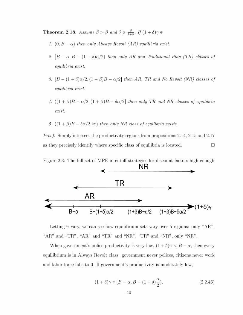
Figure 2.3: The full set of MPE in cutoff strategies for discount factors high enough

(1+β)B−δα/2(1+δ)γ

B−α B−(1+δ)α/2 (1+β)B−α/2

AR

NR

TR

Letting γ vary, we can see how equilibrium sets vary over 5 regions: only “AR”,

“AR” and “TR”, “AR” and “TR” and “NR”, “TR” and “NR”, only “NR”.

When government’s police productivity is very low, p1` δqγ ă B ´ α, then every

equilibrium is in Always Revolt class: government never polices, citizens never work

and labor force falls to 0. If government’s productivity is moderately-low,

p1` δqγ P rB ´ α,B ´ p1` δqα

2q, (2.2.46)

40

then AR equilibria as well as history-dependent Traditional Play equilibria exist. If

the old worked, then the government polices and the young work, and thus the labor

force remains at 1. But if the old revolted, then the government gives up and the

young revolt, and thus labor force remains at 0. Here, the labor force in the low state

is always 0 and labor force in the high state depends on equilibrium.

If government’s productivity is moderate,

p1` δqγ P rB ´ p1` δqα

2, p1` βqB ´

α

2s, (2.2.47)

then AR and TR equilibria still exist and also No Revolt (NR) equilibria are al-

lowed: government always polices and citizens always work and labor force rises to

1. Here labor force in both states is indeterminate and depends on equilibrium. If

government’s productivity is moderately-high,

p1` δqγ P pp1` βqB ´α

2, p1` βqB ´ δ

α

2s, (2.2.48)

then AR equilibria disappear and only TR and NR equilibria remain. Here labor

force in the low state is indeterminate and labor force in the high state rises to 1.

Finally, if government’s productivity is very high,

p1` δqγ ą p1` βqB ´ δα

2, (2.2.49)

then NR is the only equilibrium class that is allowed. Here labor force in both states

rises to 1.

41

Among all equilibria, the highest cutoffs are seen for the greatest AR equilibrium

12:

tp˚ “ p0, 0q, c˚ “´

p1` βqB, p1` βqB ´α

2

¯

u (2.2.50)

Likewise, the lowest cutoffs are seen for the smallest NR equilibrium13:

tp˚ “ c˚ “´

B ´α

2, B ´ α

¯

u (2.2.51)

The following corollary observes that one of these two extreme extreme equilibria

always exists. Naturally, low γ – unproductive police can always sustain the highest

AR, high γ – productive police can always sustain the lowest NR. The cutoffs in

these equilibria independent of γ. Intermediate γ can sustain both as well transient

TR equilibria that are not robust and depend on γ.

Recall 2.2.45 that

β “´1`

b

1` 42Bα´1

2P p0, 1q (2.2.52)

Corollary 2.19. Assume β ą β. Then for every γ, at least one of the following is

an equilibrium: tgreatest cutoff AR, smallest cutoff NRu.

Proof. By Theorem 2.18, there is either NR or AR equilibrium (or both). By Propo-

sitions 2.3 and 2.5, those are the respective robust equilibria.

2.3 Police Productivity γ with a Downward Trend

In the previous analysis, γt “ γ police productivity was constant over time. Instead,

consider a downward trend in γt ą 0 over time. This can be interpreted as police

12Without policing tomorrow, thresholds today are especially high13Policing infinitely into the future keeps thresholds today especially low

42

becoming less effective per dollar invested over time. The law enforcement and the

military are defecting to the opposition, making marginal policing more expensive.

Assumption 2.20. Public knowledge about tγtu8´8 sequence.

Assumption 2.21. Downward trend γt ě γt`1.

Assumption 2.22. Initial (high-productivity region DL : p1` δqγL ą p1` βqB

Assumption 2.23. αBă mint 1´β2

1` 12β, 2βp1´β2q

1`β´β3 u P p0, 0.55q

Assumption 2.24. Eventual low-productivity region

DN : p1` δqγN ă p1´ β2qB ´ α

ˆ

1`β

2

˙

Assumptions 2.22 and 2.24 will establish extreme dominance regions to “Never

Revolt” initially and “Always Revolt” eventually, respectively.

Next, Assumption 2.23 is a technical requirement to prove sufficiency for some of

the results (it is not a necessary restriction). αBă

1´β2

1` 12β

ensures p1´β2qB´αp1` β2q ą

0, and thus Assumption 2.24 is well-defined. This stems from considering the lowest

possible best-response level of policing required and government not being able to

afford that level. The second part of Assumption 2.23, αBă

2βp1´β2q

1`β´β3 will be used to

prove the non-monotonicity result in Theorem 2.31.

The government is a long-lived player with 0 ă δ ă 1 discount and citizens are

short-lived, asummed to live for two periods with 0 ă β ă 1 discount. There is a

measure 12

of citizens that are born every period and commit to an action a P t0, 1u

for both periods, where a “ 0 represents “protest” or “joining the opposition” and

a “ 1 represents “work.” Citizens are “Young” when they are born and decide their

action and are “Old” when they are stuck playing what they chose last period.

At the beginning of period t, the government observes the average action of the

Old ao before picking a policing level pt P r0,8q. Focusing on the symmetric pure

43

strategies, ao P t0, 1u. Then the Young are born and they observe both pao, ptq before

picking work or protest a P t0, 1u. The labor force is the total amount of work done

by the Old and the Young combined,

Lt “ p1{2qao` p1{2qay. (2.3.1)

The labor force is restricted to t0, 12, 1u for symmetric equilibria in pure strategies.

Government’s Markov strategy in state pa, tq, the Old’s average work level and

time t, is the policing level:

ppa, tq : t0, 1u ˆNÑ r0,8q (2.3.2)

(Young) citizen’s Markov strategy in state pa, p, tq, which is the Old’s work level

and government policing level, is the choice between protest and work:

apa, p, tq : t0, 1u ˆ r0,8q ˆNÑ t0, 1u (2.3.3)

We are still going to use Markov Perfect Equilibrium in pure strategies as the main

solution concept, with the added generation of using time t as one of the states. A

pair of Markov strategies (a˚, p˚) are MPE when they withstand one-shot deviation

in every state.

Again, restricting attention to citizens playing a threshold strategy this can be

rewritten as tpc˚,t0 , c˚,t1 qut:

a˚pa, p, tq “

$

’

’

&

’

’

%

1 if p ě c˚,ta ,

0 if p ă c˚,ta ,

(2.3.4)

44

Government utility from p˚, taking tpct0 , ct1qut as given, at state a and at time t

is

Gtpa|p˚q “ p1´ δq

ˆ

a

2`1tp˚,ta ěctau

2´

1

2γp˚,ta

˙

` δGt`1p1tp˚,ta ěctau

q|p˚q (2.3.5)

Denote government utility from one-shot deviation to p P r0,8q and later going

back to p˚ as

Gtpa|p˚q “ p1´ δq

ˆ

a

2`1tpěctau

2´

1

2γp

˙

` δGt`1p1tpěctau|p

˚q (2.3.6)

Taking tpct0, ct1qut as given, government’s choice tpp˚,t0 , p˚,t1 qut is optimal for every a P

t0, 1u, for every t P N, for every deviation p P r0,8q :

p1´ δq

ˆ

1tp˚,ta ěctau

2´

1

2γp˚,ta

˙

` δG´

1tp˚,ta ěctau

, t` 1¯

(2.3.7)

ě p1´ δq

ˆ

1tpěctau

2´

1

2γp

˙

` δG`

1tpěctau, t` 1˘

Corollary 2.25. Suppose citizens follow c˚-strategy, then government’s best-response

from Eq. (2.3.7) in state pa, tq is p˚,ta P t0, c˚,ta u.

Proof. Note that proof of Lemma 2.10 applies here because continuation value Gp1, t`

1q is the same for p and c˚,ta whenever p ě c˚,ta and Gt`1p0q for 0 and p ă c˚,ta , so pick

policing that gives lowest cost today and the same continuation.

Suppose in state pa, p, tq with other citizens following prescribed c˚-strategy with

p ě c˚,ta and government follows p-strategy, the young citizen also prefers to work over

protest if:

p ě p1` βqB ´ α

˜

1` β

2`a

2`β1

tpt`11 ěc˚,t`1

1 u

2

¸

´ βpt`11 (2.3.8)

45

The above condition on work, a “ 1, to be a collectively sustained citizen best-

response holds for all p ě c˚,ta if and only if

@a P t0, 1u, c˚,ta ě p1` βqB ´ α

˜

1` β

2`a

2`β1

tpt`11 ěc˚,t`1

1 u

2

¸

´ βpt`11 (2.3.9)

Suppose in state pa, p, tq with other citizens following prescribed c˚-strategy with

p ă c˚,ta and government follows p-strategy, citizen also prefers to protest over work

if:

p ă p1` βqB ´ α

˜

a

2`β1

tpt`10 ěc˚,t`1

0 u

2

¸

´ βpt`10 (2.3.10)

The above condition on protest being a collectively sustained best-response holds for

all p ă c˚,ta if and only if

@a P t0, 1u, c˚a ď p1` βqB ´ α

˜

a

2`β1

tpt`10 ěc˚,t`1

0 u

2

¸

´ βpt`10 (2.3.11)

The difference between LHS of (2.3.8) and (2.3.10) is that in the former case citizen

derives coordination utility of 12

from working alongside with 1{2 population of the

young today and β2

from working with 1{2 population of the old tomorrow. In the

later case, today’s young and tomorrow’s old protest instead because p ă c˚,ta .

Exactly like in the static case, to describe (2.3.9) condition, define the following

auxiliary function, ppp1, a, a1q. In this notation, a is the old’s labor choice from last

period and pa1, p1q are tomorrow’s work and policing choices after observing work

today.

ppp1, a, a1q ” p1` βqB ´ βp1 ´ α

ˆ

1` β

2`a` a1β

2

˙

. (2.3.12)

46

To describe (2.3.11) condition, define the following auxiliary function:

ppp0, a, a0q ” p1` βqB ´ βp0 ´ α

ˆ

a` a0β

2

˙

. (2.3.13)

In this notation, a is the old’s labor choice from last period and pa0, p0q are tomorrow’s

work and policing choices after observing protest today.

Given tomorrow’s play

tpt`10 , pt`1

1 , ct`10 , ct`1

1 u, (2.3.14)

define a static, collectively-sustained citizen best-response at t as an element of the

following two-dimensional region bounded by four inequalities:

BRtppt`1

0 , pt`11 , ct`1

0 , ct`11 q “ (2.3.15)

tpct0, ct1q : pppt`1

1 , a,1tpt`11 ěct`1

1 uq ď cta ď pppt`10 , a,1tpt`1

0 ěct`10 uq for a=0,1.u (2.3.16)

By construction, x P BRt is equivalent to x satisfies (2.3.9) and (2.3.11).

We can now describe the circumstances when an individual citizen has no prof-

itable unilateral deviations in all periods. Given a sequence of policing ppt0, pt1q, a

sequence of cutoffs pct0, ct1q is said to be a dynamic, collectively sustained best-response

if pct0, ct1q P BRtppt`1

0 , pt`11 , ct`1

0 , ct`11 q for all periods t. The distinction is that the

static requirement only makes sure today’s cutoffs work given tomorrow’s policing

and tomorrow’s cutoffs. The dynamic requirement also needs to make sure that yes-

terday’s play is consistent with today’s cutoff. It is possible that some cutoff pcT0 , cT1 q

satisfies BRt but there is no sequence tc0, c1ut satisfying BRt for all t, coinciding at

T : cT0 “ ct0, cT1 “ cT1 .

47

By construction, (2.3.8) part of BR is violated if c˚,ta ă pppt`11 ,1

tpt`11 ěc˚,t`1

1 uq

and (2.3.10) part of BR is violated if c˚,ta ą pppt`10 , a,1

tpt`10 ěc˚,t`1

0 uq, hence this is a

necessary condition.

The following lemma is similar to Proposition 2.12 but now c˚,ta ‰ c˚,t`1a (citizen

thresholds may or may not be equal across time), which allows more varied labor

behavior tomorrow to be consistent with some best-response threshold today for any

β P p0, 1q. For example, Counter-culture tomorrow requires c˚,t`10 ď α

2β, which is

small for large β, while every c˚,t0 satisfying BR at t is always large because pt`11 “ 0.

This is why in the static case requiring thresholds to be constant over time lead to

breaking BR at today when CC is played next period. Thus the dynamic thresholds

allow for new kind of equilibrium action CC, with revolt in a good state and working

in a bad state, that was eliminated under “reasonably high” patience with stationary

strategies.

Define the length of side of the BR set along a as:

∆t“ pppt`1

0 , a, a0q ´ pppt`11 , a, a1q “ βppt`1

1 ´ pt`10 q ` α

ˆ

p1` βq

2`βpa1 ´ a0q

2

˙

(2.3.17)

The second effect of letting thresholds vary over time is that the shape of

tpc˚,t0 , c˚,t1 q: satisfying BRtpp˚,t`10 , p˚,t`1

1 q conditions at every tu is a square. Previ-

ously the restriction of time-stationary thresholds would lead to downward sloping

boundary for small c˚0 . With exogenously fixed pc˚,t`10 , c˚,t`1

1 q the shape is a rectangle

and ∆t, the length of the side, is independent of a, so it is a square with lower-left

corner at

ppppt`11 , 0,1

tp˚,t`11 ěc˚,t`1

1 uq, ppp˚,t`1

0 , 1,1tp˚,t`1

1 ěc˚,t`11 u

qq (2.3.18)

48

and upper-right corner at

ppp˚,t`10 , 0,1

tp˚,t`10 ěc˚,t`1

0 uq, ppp˚0 , 1,1tp˚,t`1

0 ěc˚,t`10 u

qq. (2.3.19)

Lemma 2.26. Suppose at time t`1 the government plays Never Revolt (NR), Always

Revolt (AR), Traditional Play (TR) or Counter-culture (CC) that pins tomorrow

young’s action at pa0, a1q14. Then pc˚,t0 , c˚,t1 q satisfies BRtpp˚,t`1

0 , p˚,t`11 q if and only if

ppp˚,t`11 , a, a1q ď c˚,ta ď ppp˚,t`1

0 , a, a0q

Outline. The result is similar to Proposition (2) but the proof is much simpler because

next period’s cutoffs depend on t ` 1 and are uncoupled from today’s cutoffs. This

follows straight from the definition of 2.3.17.

The above Lemma means you only need to know tomorrow’s policing and tomor-

row old’s profile of equilibrium actions in each state a P t0, 1u to verify pc˚,t0 , c˚,t1 q P

BRtpp˚,t`10 , p˚,t`1

1 q – in other words, today’s cutoffs are independent of each other as

long as the corresponding equilibrium policing levels don’t violate feasibility at t´ 1,

in other words that BRt´1pp˚,t0 , p˚,t1 q ‰ H (see next Lemma).

The following lemma gives a necessary and sufficient condition on play at t` 1 to

ensure BR set at t is non-empty or equivalently ∆t ě 0. It cannot be the case that

c˚,t`11 ! c˚,t`1

0 as that moves lower boundary of BR at t above upper boundary of BR

at t, making BR empty.

Lemma 2.27. Dtpc˚,t0 , c˚,t1 qu satisfying BRtpp˚,t`10 , p˚,t`1

1 q if and only if (∆t ě 0)

p˚,t`11 ´ p˚,t`1

0 ě ´α

2β

´

1` β ` βp1tp˚,t`1

1 ěc˚,t`11 u

´ 1tp˚,t`1

0 ěc˚,t`10 u

q

¯

14The subscript i indicates that the current young’s action is i. Therefore, tomorrow’s young willobserve i before making their choice, ai “ 1

tp˚,t`1i ěc˚,t`1

i u.

49

Proof. See Appendix.

The previous Lemma highlights the desired restriction on next the period’s polic-

ing levels. It cannot be too high in the bad state relative to good state, or BR

conditions fail for the previous period. This is similar to how we eliminated Counter-

Culture (CC) equilibria in the stationary case.

The following proposition defines a special “FP” fixed-point set of BR thresholds

for Never Revolt (NR) play. If a sequence of thresholds satisfy BR and some point

later in the sequence is in “FP,” then every point before that is also in FP. But

even if none of the points are in “FP”, as the sequence gets longer, the first point

pc˚,t“10 , c˚,t“1

1 q is arbitrarily close to FP’s boundary. In other words, whenever govern-

ment polices within this boundary (a moderate amount), then it policed inside the

boundary every period before that. And every sequence of positive policing support-

ing NR play, always starts arbitrarily close to the boundary if the sequence is long

enough.

The following expression P a is the maximum possible positive policing in any

MPE in state a, when today’s young are pessimistic15, the following period will have

no policing and tomorrow’s young will protest:

P a “ pppt`1“ 0, a, a0 “ 0q “ p1` βqB ´ α

a

2(2.3.20)

Likewise, the following expression P a is the minimum possible positive policing in

any MPE in state a, when today’s young are optimistic16 the following period will

15Protest is dominant above any lower policing level, by expecting full mutual protest in such acase.

16Work is dominant below any higher policing level, by expecting full mutual protest in such acase.

50

have maximum policing P a and tomorrow’s young will work:

P a “ pppt`1“ P a, a, a0 “ 1q “ p1´ β2

qB ´ α

ˆ

1` a` β

2

˙

(2.3.21)

Proposition 2.28. Suppose Never Revolt (NR) is played for t ď L. The following

BR set, denoted as “FP”, is the smallest fixed-point set.

1. If β P p0, 12q : “FP”=

„

B ´αp1` β ´ β2q

2p1´ β2q, B `

αβ2

2p1´ β2q

ˆ

„

B ´αp2` β ´ 2β2q

2p1´ β2q, B ´

αp1´ 2β2q

2p1´ β2q

2. If β P p12, 1q : “FP”=

„

B ´αp1` β ´ β2q

2p1´ β2q, B `

αβ2

2p1´ β2q

ˆ

„

B ´αp2` β ´ 2β2q

2p1´ β2q, B ´

αp1´ 2β2q

2p1´ β2q

Xtpp0, p1q : Lemma (2.27) holds.u

Proof. (OUTLINE) 1. BR set at t´ 1 Ă BR set at t. (i) ppp˚,t´11 , a, 1q ě ppp˚,t1 , a, 1q

and (ii) ppp˚,t´10 , a, 1q ď ppp˚,t0 , a, 1q This means once you start in that square region,

then you stay there.

The second restriction for β P p0.5, 1q ensures p0 ! p1 doesn’t happen.

To show that this is the unique FP: any BR set at t that contains the BR set at

t ´ 1, also contains “FP.” As L Ñ 8, the candidate set shrinks to FP arbitrarily

close (pick any BR point outside of FP at t “ 2, it is no longer contained in BR set

at t “ 1 for L large enough).

To show that it has no “slack,” pick top left corner. BR set at t´ 1 starting there

is “FP.” The size of “FP” square ∆ “ α2p1´βq

51

Observation: ∆t´1, size of the BR set the previous period increases in ∆pt - the

difference in policing levels at t. This difference in policing levels is maximized at the

top left corner of any BR set. Starting with a larger candidate for “FP”, shrinks the

BR set strictly the period before: if ∆t ą α2p1´βq

ùñ ∆t´1 ă ∆t. Similarly, starting

with a smaller candidate for “FP”, grows the BR set strictly the period before: if

∆t ă α2p1´βq

ùñ ∆t´1 ą ∆t. This shows “FP” is the unique such set.

The interpretation of the Fixed-Point set is it’s precisely the set of policing levels

that are feasible under Never Revolt equilibrium with infinite horizon (e.g. if γ always

remained in the upper-dominance region).

Proposition 2.29 (Opposition eventually takes over). 1. (Lower Dominance Region)

Consider subgame starting at pN, aq.17Unique labor outcome is “Always Revolt” for

every Markov Perfect Equilibrium for this subgame : p˚,ta “ 0 ă c˚,ta .

2. (Contagion) Extend the subgame above to a supergame pt “ K ď N, aq such

that p1` δqγK ă p1`βqB´α`

1` β2

˘

. for every Markov Perfect Equilibrium for this

subgame : @t ě N : p˚,ta “ 0 ă c˚,ta .

Proof. See Appendix.

Similar to the stationary dynamic model, there are four possible equilibrium labor

outcomes in a given period. The above proposition established a contagion argument

where forward-looking (pessimistic) expectations lead to a unique labor outcome of

Always Revolt. Previously, it was only the case that AR was unique for p1 ` δqγ ă

B ´ α and allowed for multiplicity from TR and NR above that.

Now, the NR region has been extended to

p1` δqγ ă p1` βqB ´ α

ˆ

1`β

2

˙

(2.3.22)

17From Asmp 4, p1` δqγN ă p1´ β2qB ´ α

´

1` β2

¯

“ P 1

52

Looking at it another way, the stationary model had multiplicity on a region with

width increasing in βB, the cost of work, plus a factor proportional to α, because with

stationary policing strategy tomorrow’s policing was correlated with today’s policing.

In the dynamic model with a downward trend, the multiplicity region has width

proportional to α only, coordination among the citizens only. This is a qualitative

sense in which the indeterminacy has been reduced.

The next theorem focuses on describing a general pattern present in any equilib-

rium with a downward productivity trend. The first stage is “Tyranny” where the

government enforces work in every period for a while.

It is followed by a turbulent stage called “Revolution” and for a given productivity

trend, different equilibria allow for different paths taken on this region. If citizens

coordinate on instant revolution, they could have it on the first day of the period or

at the other extreme, instead, they could coordinate to do it on the last period with

some specified play in the interim. This is consistent with the literature where timing

of the revolution in the short-run is somewhat indeterminate, even when it is certain

to happen in the long-run.

The final stage is called “Opposition in Power” and it corresponds to the govern-

ment completely giving up forever, never policing and citizens always revolting.

Theorem 2.30. Consider γt satisfying Asmp 1-5. Let L “ maxltp1 ` δqγl ą p1 `

βqBu, the last period in the upper dominance region. Fix any MPE equilibrium.

1. (TYRANNY) The first L ą 0 periods have Never Revolt (NR) outcome.

2. (REVOLUTION) Next k ě 0 periods play one of tNever Revolt (NR), Always

Revolt (AR), Traditional play (TR), Counter-culture (CC) u

3. (OPPOSITION IN POWER): The infinite tail starting from K “ L ` k ą 0,

has Always Revolt (AR) outcome.

53

Proof. 1. At t “ L, the worst case scenario is the government faces infinite tail of

Always Revolt starting next period at t “ L ` 1. From the first column of Table 1,

playing p “ c˚,La gives strictly greater payoff than playing p “ 0 ðñ c˚,La ă p1`δqγL.

This is true because c˚,La ď p1` βqB ă p1` δqγL

3. This follows from Proposition 2.29. Let

K “ mink

"

p1` δqγk ą p1` βqB ´ α

ˆ

1`β

2

˙*

2. This follows directly from Corollary 4.1 and k “ K ´ L depends on K, when the

contagion kicks in.

The final result establishes the non-monotonicity of policing result for the dynamic

model with a trend. While the previous Theorem 2.30 focused on how anticipation of

future play affected the labor path, Theorem 2.31 looks at how every equilibrium labor

path affects government’s equilibrium policing response. An important contribution

of this paper is to highlight the following pattern.

On the period before the revolution begins: (i) the tomorrow’s old protest, which

discourages work today, (ii) continuation utility of receiving policing tomorrow be-

comes zero since the government gives up, also reducing payoff to work. These two

factors cause a discontinuous drop in relative utility of work, so today’s policing

needs to be higher by a discrete increase to compensate. Less policing is needed to

incentivize work where for many future periods there is going to be a guarantee of

tomorrow’s old working, plus a positive amount of policing tomorrow.

This means when the government had held the power firmly a long time ago,

early in the “Tyranny” region, it policed a moderate amount. On the last period

of “Tyranny” before “Revolution,” it must police a lot more, else protests would

have started even earlier. The government subdues mild opposition with mild polic-

54

ing, deters strong opposition with heavy policing and gives up against unstoppable

opposition at the start of the final region where “Opposition is in Power.”

Theorem 2.31 (Non-monotonicity of policing in γ). Consider γt satisfying Asmp

1-5 and for every MPE, there exist time periods M and T, pM ă T q, that exhibit

non-monotonicity of observed policing with respect to γ.

0 “ p˚,T1 ă p˚,M1 ă p˚,T´11

Proof. See Appendix.

2.4 Conclusion

This paper extends the literature on protests and revolutions to include government

as a strategic agent. Choosing to highlight time frictions, rather than informational

frictions, the model makes a connection between anticipation of inevitable revolution

and non-monotonic government’s policing.

The dynamic model allows for forward-looking expectations to reduce equilibrium

indeterminacy by using a downward trend of police productivity. On one hand, it

fully characterizes the different kinds of Markov equilibrium labor paths that arise in

a repeated game. On the other hand, it makes a prediction that the government will

police mildly when its power is secured, give up when the opposition is too strong and

fiercely fight back when its government’s rule is about to collapse, even if the collapse

is inevitable. This roughly matches the Imperial Russian government’s response to

the Socialist opposition. First it used spies, imprisonment and exile. Then when

its rule was in peril, it crushed striking civilians with artillery bombardment. Next

time, however, its policing effectiveness has declined and it could not oppose the

revolutionaries.

55

The model with stationary police productivity gives a short-run analysis of poten-

tial protests. Later, police productivity is described by a deterministic (downward)

trend. This gives a long-run analysis of how anticipation of eventual fall of govern-

ment brings about certain revolution. This revolution will happen at an earlier time

than is likely in the short-run model without aligned expectation of its fall. Still, the

exact date of the revolution is unpredictable and may vary across equilibria, which is

consistent with the widespread surprise of the Berlin Wall collapsing.

In the stationary case with high police productivity, the government’s costly ac-

tion can force coordination on its preferred outcome of work, retaining power. For

the stationary low police productivity, the government cannot afford to cover indi-

vidual citizen’s fixed cost of work and there are always protests and never policing.

Therefore, the government loses control to the rebel opposition. In the intermediate

regions, there are also possible outcomes of Traditional Play, where rebels’ children

protest and workers’ children work. However, much of this is resolved by a downward

trend as an Always Revolt outcome by contagion.

An extension for this line of research would be to model the government-opposition

game as “matching pennies” where the citizens want to allocate themselves across

time or place (a clandestine meeting), preferring to be together but to avoid the

government. Meanwhile, the government uses a finite policing budget to allocate its

police to minimize the oppositions’ gatherings as much as it could.

56

Chapter 3

Reference-Dependent Attitudes to

Risk, Incumbency Advantage and

Response to Crisis

The political science literature has identified a salient phenomenon known as incum-

bency advantage, where politicians in office stand a higher chance of being reelected

than challengers vying for the same seat. Conventional explanations include deter-

rence of challengers, lower quality of challengers than incumbents (incl. incumbents

having political experience), use of office for reelection (e.g. franking letters, greater

access to media, pork-barrel spending).

Secondly, more recent research has described the opposite circumstance of incum-

bency disadvantage when challengers do better in bad times after an exogenous shock

to the economy, which is unrelated to the government’s actions.

A non-conventional explanation using prospect theory may be able to explain

both incumbency advantage during good times and incumbency disadvantage during

a time of crisis, when the loss-gains function is strictly concave with risk-seeking in

the losses and risk-aversion in the gains.

57

The third stylized fact is that while incumbent’s average disaster relief increases

in the magnitude of the (exogenous) crisis, their average probability of winning de-

creases. In other words, an average incumbent wins more often when he is lucky to

avoid an unrelated crisis and loses more often when he is not lucky, while providing

the expected disaster relief for that particular crisis. Thus, these election patterns

cannot be explained by backward-looking voters who punish only lazy politicians for

underperformance.

Over 90% of House Representatives seeking reelection were successful since World

War II (Levitt and Wolfram, 1997). Gelman and King (1990) developed the first

consistent and unbiased measure in terms of vote percentage margins, constructing

a proper time-series for congressional elections. They found the average incumbency

advantage to be 2% between 1900 and 1950, then steadily rising to about 10% in

1990. In fact, Levitt and Wolfram (1997) found that deterrence trumps officeholder

benefits, including free mail, media access, fund-raising advantages to explain the rise

of incumbency advantage post-World War II.

Ansolabehere and Snyder Jr (2002) showed that incumbency advantage exists at

a similar level (co-movements over time) at state and federal legislatures, guberna-

torial and other state executives. Therefore, these phenomena do not depend on

specific from features of the legislature like redistricting (gerrymandering), diffusion

of responsibility or pork-barrel politics because similar incumbency advantage ex-

ists in elections for offices without these specific benefits. The proposed decline in

challenger quality was also rejected as an explanation for the rise in incumbency ad-

vantage. There has to be a more general explanation that applies both to legislatures

and the executive.

More recently, Wolfers (2007) analyzed comprehensive empirical evidence that

voters reelect incumbents during good times (high oil prices for oil-producing states,

national boom for pro-cyclical states) and elect challengers during bad times. One

58

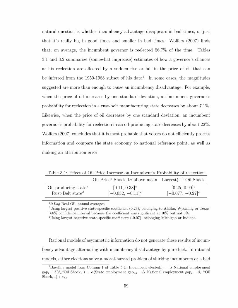
natural question is whether incumbency advantage disappears in bad times, or just

that it’s really big in good times and smaller in bad times. Wolfers (2007) finds

that, on average, the incumbent governor is reelected 56.7% of the time. Tables

3.1 and 3.2 summarize (somewhat imprecise) estimates of how a governor’s chances

at his reelection are affected by a sudden rise or fall in the price of oil that can

be inferred from the 1950-1988 subset of his data1. In some cases, the magnitudes

suggested are more than enough to cause an incumbency disadvantage. For example,

when the price of oil increases by one standard deviation, an incumbent governor’s

probability for reelection in a rust-belt manufacturing state decreases by about 7.1%.

Likewise, when the price of oil decreases by one standard deviation, an incumbent

governor’s probability for reelection in an oil-producing state decreases by about 22%.

Wolfers (2007) concludes that it is most probable that voters do not efficiently process

information and compare the state economy to national reference point, as well as

making an attribution error.

Table 3.1: Effect of Oil Price Increase on Incumbent’s Probability of reelection

Oil Pricea Shock 1σ above mean Largestp`q Oil Shock

Oil producing stateb r0.11, 0.38sc r0.25, 0.90sc

Rust-Belt stated r´0.032, ´0.11sc r´0.077, ´0.27sc

a∆Log Real Oil, annual averagesbUsing largest positive state-specific coefficient (0.23), belonging to Alaska, Wyoming or Texasc68% confidence interval because the coefficient was significant at 10% but not 5%.dUsing largest negative state-specific coefficient (-0.07), belonging Michigan or Indiana

Rational models of asymmetric information do not generate these results of incum-

bency advantage alternating with incumbency disadvantege by pure luck. In rational

models, either elections solve a moral-hazard problem of shirking incumbents or a bad

1Baseline model from Column 1 of Table 5.C: Incumbent electeds,t = λ National employmentgapt ` δpβs*Oil Shockt ) + α(State employment gaps,t ´∆ National employment gapt ´ βs *OilShocks,tq ` εs,t

59

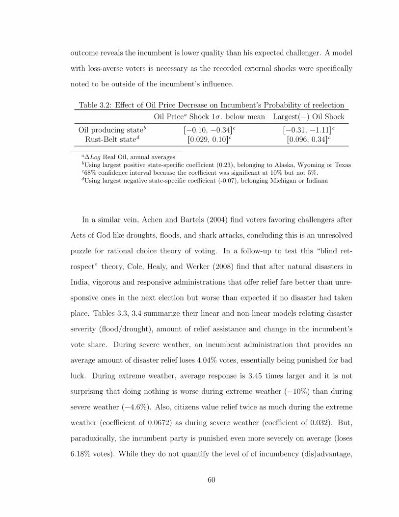
outcome reveals the incumbent is lower quality than his expected challenger. A model

with loss-averse voters is necessary as the recorded external shocks were specifically

noted to be outside of the incumbent’s influence.

Table 3.2: Effect of Oil Price Decrease on Incumbent’s Probability of reelection

Oil Pricea Shock 1σ. below mean Largestp´q Oil Shock

Oil producing stateb r´0.10, ´0.34sc r´0.31, ´1.11sc

Rust-Belt stated r0.029, 0.10sc r0.096, 0.34sc

a∆Log Real Oil, annual averagesbUsing largest positive state-specific coefficient (0.23), belonging to Alaska, Wyoming or Texasc68% confidence interval because the coefficient was significant at 10% but not 5%.dUsing largest negative state-specific coefficient (-0.07), belonging Michigan or Indiana

In a similar vein, Achen and Bartels (2004) find voters favoring challengers after

Acts of God like droughts, floods, and shark attacks, concluding this is an unresolved

puzzle for rational choice theory of voting. In a follow-up to test this “blind ret-

rospect” theory, Cole, Healy, and Werker (2008) find that after natural disasters in

India, vigorous and responsive administrations that offer relief fare better than unre-

sponsive ones in the next election but worse than expected if no disaster had taken

place. Tables 3.3, 3.4 summarize their linear and non-linear models relating disaster

severity (flood/drought), amount of relief assistance and change in the incumbent’s

vote share. During severe weather, an incumbent administration that provides an

average amount of disaster relief loses 4.04% votes, essentially being punished for bad

luck. During extreme weather, average response is 3.45 times larger and it is not

surprising that doing nothing is worse during extreme weather (´10%) than during

severe weather (´4.6%). Also, citizens value relief twice as much during the extreme

weather (coefficient of 0.0672) as during severe weather (coefficient of 0.032). But,

paradoxically, the incumbent party is punished even more severely on average (loses

6.18% votes). While they do not quantify the level of of incumbency (dis)advantage,

60

they do note that rainfall (“luck”) is relevant for deciding the winner because a quarter

of elections in their sample have margin smaller than 5.26%.

Table 3.3: Effect of Variable Rain on Disaster Relief and Votes for Incumbent Party

Expenditurea per σ of Rain ∆ Vote(%)away from Optimal Rainb

No Response 0 ´3.77%Ave. Response 0.178 ´3.25%

2x ave. Response 0.356 ´2.73%

aA governmental response is an increase in log(disaster spending)bOptimal rain is computed to be about 1 standard deviation (σ) above average, where farming

output is at maximum

It thus appears that there is a robust puzzle that incumbency advantage vanishes

during a time of crisis, even if the crisis has nothing to do with the incumbent. Sec-

ondly, disaster relief increases in the magnitude of the crisis, while the incumbent is

disadvantaged and only extreme responses merit reelection. Conventional explana-

tions either should continue to hold (e.g. if pork-barrel spending was the cause) or

are inadequate (e.g. principal-agent arguments about effort or quality with rational

voters). This paper takes the stance that when the loss-averse voters experience a

sudden cut to their consumption, the required minimum ability cutoff for the incum-

bent rises. When, in equilibrium, the average disaster relief reveals the incumbent

to have an average ability, he is then disadvantaged at the election, relative to a

risky prospect of the unknown challenger. It takes an extreme performance from the

incumbent to reveal extremely high ability to pass the muster.

This paper develops a model to explain all of these facts by linking politicians with

career concerns and forward-looking voters with reference-dependent utility. (Holm-

strom, 1999) developed a framework of moral hazard (with symmetric information)

where the agent was considered for a promotion based on their unknown ability and

61

Table 3.4: Non-linear Effect of Rain on Disaster Relief and Votes for Incumbent Party

Severe Weathera Extreme Weatherb

Exp.c ∆ Vote(%) Exp. ∆ Vote(%)

No Response 0 ´4.57% 0 ´9.99%Ave. Response 0.1641 ´4.04% 0.5663 ´6.18%

2.62x ave. response 0.4306 ´3.19% 1.486 0

aSevere Weather accounts for rainfall difference from optimal amount in 80-90 percentilesbExtreme Weather accounts for rainfall difference from optimal amount in 90-100 percentilescA governmental response is an increase in log(disaster spending)

took a hidden action, such as effort, that potentially clouded inference about their in-

nate ability. While in some equilibria it may be the case that the agent’s action ended

up revealing his ability after-the-fact, his initial incentives involved considerations to

improve the signal by exerting some additional effort.

Whether voters are assumed to be loss-averse or rational expected-utility max-

imizers, a politician will want to provide a non-trivial amount of the public good

before the election. The incumbent will take a less-than-maximal personal rent, be-

cause raising the rents further would make them look bad as if they had low ability

to create the public good. Thus, the politician does not want to reduce his ex-ante

probability of winning by shirking. With rational voters, politicians only care about

affecting signals that relate to their ability and ignore, for example, exogenous shocks

to voters’ future income, because their probability of winning only depends on the

manifestation of their own ability.

Secondly, even if the politicians had no hidden action to take (such as fixed or

zero personal rents) and the incumbent’s type was public information, that simpler

model would still generate incumbency advantage in good times and incumbency

disadvantage in bad times. The uncertainty about the challenger’s ability, relative to

the better-known incumbent, plus prospect theory gives the result.

Combining both aspects in one model leads to “fickle” voters that take into ac-

count irrelevant signals as long as their consumption relative to the reference point

62

is affected. When reference-dependence is combined with career concerns, the third

stylized fact is also matched. Thus, politicians signal higher ability when they vary

their hidden action relative to these irrelevant signals since these now enter into their

probability of winning, even though in equilibrium their type is revealed anyway.

In this case, the incumbent provides greater disaster relief when the crisis wors-

ens as the voters are risk-seeking and lean more and more towards the challengers.

Incumbents increase public goods g˚1 in the first period precisely when their proba-

bility of losing increases. Their decision involves trade-off between personal rent and

increasing probability of being elected by choosing a higher signal. In equilibrium,

all incumbents’ signals are perfectly correlated with their ability, so their type be-

comes known. However, a simpler model without career concerns that has known

incumbent’s type does not have the tension between choosing signal to affect margin

of the probability of winning, thus more public goods wont necessarily be provided

for rising moderate shock s. On the other hand, when the crisis does not occur, the

incumbent produces less of the public good and takes more personal rents by enjoying

his incumbency advantage.

A possible explanation for incumbency advantage via prospect theory was first

proposed by Quattrone and Tversky (1988), described in terms of classroom ques-

tionnaires and psychology intuition. The questions included policy proposals by can-

didates, framed in terms of losses and gains for separate groups of responders. Instead

of using expected-utility, consumers were supposed to be loss-averse with respect to

a particular, given reference point. With an S-shaped value function, they are risk-

seeking in the losses region and risk-averse in the gains region. If the incumbent

represents the continuation of the status quo and the challenger is a risky gamble,

then the incumbent should tend to get more support, except during bad times (with

risk-seeking to attempt recouping losses). However, this modelling device of loss-

averse voters has not been theoretically developed into an equilibrium model beyond

63

validation in simple classroom experiments. Prior to the present paper, this direction

has not been pursued in the literature on incumbency advantage. Since Quattrone and

Tversky (1988) hah not constructed an equilibrium model, they made no predictions

about the government’s disaster-relief response to the presence of these loss-averse

voters.

While explaining the vulnerability of incumbency advantage to economic and out-

side shocks, a limitation of this approach is that it may be challenging to explain the

positive trend in the magnitude of the incumbency advantage.

Loss aversion has been used to offer an alternative explanation for why the Pres-

idents party tends to lose seats in midterm congressional elections (Patty, 2006).

Outside of political economy, Fershtman (1996) used prospect theory in IO to demon-

strate that variation in the reference points affects market decisions of incumbent and

challenger firms, changing the market equilibrium in a dynamic oligopoly game.

The proposed theoretical model needs to go beyond assuming the challenger is

riskier than the incumbent. The model requires assumptions about the political com-

petition and information structure to endogenously generate the structure of pay-offs

where reference-dependence will be relevant. For example, Patty (2006) emphasizes

non-representative turn-out differences during midterm Congressional election, stem-

ming from the particular framing of seats in terms of losses and gains.

3.1 Career concerns and loss-averse voters

The model has two separate, but related, parts: (I) loss-averse voters have reference-

dependent utility that generates incumbency advantage in good times and disadvan-

tage in bad times, (II) “Career-concerned” politicians vary in ability and they want

to look good before the election by providing a non-trivial amount of the public good

by not shirking. Having (II) in addition to (I) lets politicians respond to signals irrel-

64

evant for determining their ability that affect voters’ consumption. As the incumbent

becomes disadvantaged with risk-seeking voters having their consumption in a loss-

region, politicians increase expenditure on the public goods, so they don’t look bad

before the election.

A starting point is to use endogenous formation of the reference point as in Koszegi

and Rabin (2007) and apply it to a model of post-election politics. That framework

uses a mix of expected utility component and a gain-loss function of prospect theory,

where the innovation is that reference-point is formed with forward-looking rational

expectations. Taking equilibrium behavior of voters and the incumbent as given (to

be described later), voters form a reference point for lottery of the consumption that

they rationally expect to receive after the election as a function of the incumbent’s

state2. This reference point will be used when the voters come to the polls and weigh

different outcomes resulting from their choice.

The baseline structure of the model is similar to the two-period “career concerns”

agency model (Persson and Tabellini, 2002). The incumbent wants to impress voters

with his quality in the first period, so they reelect him again. This signalling is

expensive and requires a cut to politicians’ personal rents. The present paper adds

the concept of a reference-dependent personal equilibrium (Koszegi and Rabin, 2007)

to the voter preferences.

First, I characterize the representative voter’s personal equilibrium and incum-

bent’s choice of provision of public goods and extraction of political rents. The

reference-point consumption lottery describes citizens’ expected consumption next

period before the election takes place. It is the weighted sum of getting the challenger-

induced consumption with probaiblity q and incumbent-induced consumption with

probaiblity 1´q, where q, 0 ă q ă 1, is the ex-ante rational expectation of incumbent

losing. Here q represents voters’ expectation of who is going win the election. In

2Voters anticipate to correctly derive it in equilibrium from the government’s public good pro-vision in the initial stage, so that the incumbent’s type is known when the vote takes place.

65

equilibrium, this expectation is rational and voters do pick the challenger q˚ fraction

of the time, given the equilibrium reference-point consumption lottery with q˚ weight.

Therefore, by endogenizing the rational reference point as in Koszegi and Ra-

bin (2007), the same number q˚ parametrizes both the reference-point consumption

lottery and incumbent’s probability of losing. We can now describe incumbency ad-

vantage and disadvantage in terms of the same q˚.

q˚ is said to characterize incumbent’s advantage for q˚ ă 12

and incumbency disad-

vantage for q˚ ą 12. The main finding of Theorem 3.1 is that during good times, every

personal equilibrium has q˚ ă 12

and it captures incumbency advantage comparable

in magnitude to Gelman and King (1990)’s 2 ´ 10% estimates. This is intuitively

driven by risk-aversion to picking challenger’s consumption lottery.

Instead, suppose the reference point was feasible in the sense it was a linear

combination of consumptions induced by the challenger and the incumbent, weighted

by q, but not necessarily rational. Then Theorem 3.1 also shows there is a unique

cutoff strategy parametrized by ηq, the incumbent’s probability of losing. During

good times, for for all q, 0 ă ηq,ă12, so that there is incumbency advantage even for

irrational feasible reference points that do not form a personal equilibrium.

Suppose a voter finds it optimal to reelect incumbent in two-thirds of possible

states (of incumbent’s performance), given a reference-point compound lottery of

receiving challenger’s consumption lottery q percent of the time and receiving in-

cumbent’s consumption lottery 1 ´ q percent of the time. This would be a personal

equilibrium if only if q “ 13.

Either way, it turns out the “career-concerned” incumbent provides more public

goods when his probability of losing increases3.

Second, while fixing voter’s ERPCL, I look at how agents react to the surprise

negative shock to the voter’s income in the second period that is realized just before

3In the particular linear parametrization of this paper, the amount of the public good is directlyproportional to the probability of losing

66

the election. This shock is exogenous to the economy and specifically to incumbent’s

actions (e.g. an earthquake, flu epidemic, global economic slowdown). For tractabil-

ity, the first pass of this analysis assumes that voters assigned a zero probability to

this rare shock when they formed their equilibrium reference-point lottery before the

election. The main finding here is for small negative shocks to future income, incum-

bency advantage diminishes even without strict convexity of the gain-loss function

µ. With strict convexity in the loss region, there is incumbency disadvantage for

moderate negative shocks.

It is for the analysis of incumbency disadvantage and comparative statics where

endogenizing the reference point is especially useful. The surprise shock model takes

an equilibrium reference-point lottery from the no-shock environment and generates

a voting decision rule Qpq; sq that varies with the size of the shock s. When q ă

Qpq; sq ă 12, the incumbency advantage is said to decrease from the shock, for example

when the gain-loss function µ is piece-wise linear. Similarly, when q ă 12ă Qpq; sq, it

describes incumbency disadvantage, such as when µ is strictly convex. In both cases

the incumbent provides more public goods because Qpq; sq ą q as the probability of

losing increases.

Finally, the surprise model is extended to a model with fully rational expectations

where the negative income shock s happens with probability p, 0 ă p ă 1, and

income y remains unchanged with 1 ´ p probability. In the limit as p Ñ 0, the

rational-expectations model captures the surprise model as a special case.

3.1.1 Politicians

The government taxes voters in both periods at a constant rate τ and provides public

goods gt, t P t1, 2u. At the end of every period, voters vote in favor of the incumbent

or the single challenger. Politicians differ in their ability η to convert private goods

into public goods.

67

We will assume that this ability η is uniformly distributed on r0, 1s for all politi-

cians. That is, ex-ante the incumbents and challengers are equally skilled and the

deck is not stacked to generate incumbency (dis)advantage in an ad hoc manner by

drawing challengers from a different pool. The only distinction is that the equilibrium

play will fully reveal incumbent’s type but off-equilibrium incumbents can consider

altering their hidden action to signal a different type.

When converting one unit of private good, η units of public good are produced.

Once a new politician is picked for office, his competence η remains fixed throughout

his career (no learning-by-doing) but no one knows the value of η during his first term

(not even himself as the job is new to him). The politician will learn his competence

after one term and voters will be able to indirectly, though accurately, infer it in

equilibrium just before casting their vote. If a challenger politician is elected, ηc is

drawn from the same distribution as incumbent’s ηi.

Politicians are purely opportunistic - they only care about extracting personal

rent rt out of taxes and exogenous ego rents of being reelected, R (which may capture

continuation value of future rents).

Hence, the politician’s value function is

vI “ r1 ` βpIpr2 `Rq (3.1.1)

where pI is the probability of being elected, which is driven by voter’s decisions; rt

are the rents extracted in period t; 0 ă β ă 1 is the discount factor; R is the value of

being reelected to office.

Voters do not observe rents extracted or ηi but they judge competence based on

how many public goods were provided. Incumbent’s trade-off to extract everything

is to appear incompetent and lose election and forgo future rents. At the beginning

of every period t P t1, 2u, the incumbent balances the budget between personal rents

68

and public goods. Since in the last period (t “ 2) there is no reelection incentive,

r˚2 “ r ă yτ , the maximum allowed by feasibility.

The budget constraint for the incumbent in period t is:

ηiτy “ ηirt ` gt ùñ gt “ ηipτy ´ rtq, (3.1.2)

where the action to take is rt P r0, rs and gt is residually determined.

The information is symmetric for tractability as the principal-agent story is not

appropriate for studying exogenous shocks like an earthquake. At the same time, the

ex-ante outcome of elections is non-deterministic – the challenger has a viable chance

to win and neither politician is endowed with a competence advantage; there is no

deterrence effect here either. Since the incumbent cannot condition his personal rent

strategy r1 on own not-yet-realized type, all incumbents extract the same equilibrium

amount of rents r˚1 , so that the amount of public goods provided g1 becomes a random

variable, perfectly correlated with ηi.

3.1.2 Voters

In this model voters only care about their own consumption and do not have an

ideological party bias. Their consumption utility in period t is linear in consumption,

c, which is composed of disposable income yp1´ τq plus the public good:

mpcq “ c “ yp1´ τq ` αgt, (3.1.3)

where y ą 0 is the fixed income for both periods, 0 ă τ ă 1 is the fixed taxed rate,

α ą 1 is the preference for public goods and gt is the amount of the public goods

provided.

Koszegi and Rabin (2007) bridged the gap between expected utility and classical

prospect theory that only looks at the gains losses by considering both. Voter’s utility

69

in the period after the election is:

UpF |Gq “

ż

´

ż

upc|rqdGprq¯

dF pcq “

ż

´

ż

mpcq ` µpmpcq ´mprqqdGprq¯

dF pcq,

(3.1.4)

where F is the consumption lottery, G is any reference (consumption) lottery and

µp.q is the gain-loss function.

We will assume the following parametric form for the gain-loss function that al-

lows for linearity or strict concavity. While piece-wise linearity has been used in

previous research for tractability, risk-seeking in the losses is required to generate

strict incumbency disadvantage, rather than simply decreasing the advantage.

µpxq “

$

’

’

&

’

’

%

γx1k if x ą 0,

´γλp´xq1k if x ď 0.

(3.1.5)

where γ ą 0 is a scale parameter for gains and losses relative to the base utility

for consumption (γ “ 0 is expected utility); λ ą 1 scales the degree of loss-aversion

relative to gains; k P N is a curvature parameter: k “ 1 corresponds to non-strict

concavity and convexity of the standard piece-wise linear gain-loss function and k ą 1

allows for risk-seeking in the losses.

With only two political candidates, there is no problem of strategic voting. Unlike

principal-agent models, where voters are sometimes asked to commit to retrospective

punishment strategies, voters here are forward-looking when they select the candidate

to maximize their next period’s utility, conditional on the reference point.

The voter observes g1 before voting but not ηi. If the voter picks the incumbent,

then he will receive the degenerate consumption lottery:

ci “ yp1´ τq ` αgi2 “ yp1´ τq ` αηipτy ´ rq (3.1.6)

70

which is increasing in ηi, which will be inferred accurately in equilibrium from g1, so

ci is not a random variable.

If the voter picks the challenger, then he will receive non-degenerate consumption

lottery:

cc “ yp1´ τq ` αgc2 “ yp1´ τq ` αηcpτy ´ rq (3.1.7)

Because ηc is a random variable that has not been realized, cc is also a random

variable, which inherits the uniform distribution.

Denoting θ, θ P r0, 1s, to be the random realization of the challenger’s ability, an

arbitrary reference point is characterized by a fixed q P r0, 1s

cq “ qcθ ` p1´ qqci “ q pyp1´ τq ` θGq ` p1´ qq pyp1´ τq ` ηGq

“ yp1´ τq ` qθG` p1´ qqηG (3.1.8)

where G ” αpτy ´ rq, the public-goods production technology.

It is a lottery where the challenger’s lottery is drawn with probability q. As before,

η is the imputed incumbent’s ability from his equilibrium play. As it will be known

at the moment of the election, when considering next period’s gains and losses, the

voter will treat η as a degenerate (constant) lottery that puts mass 1 on η.

Given the reference lottery cq, the utility of voting for the challenger is evaluated

as:

Upcc|cqq “

ż 1

0

ż 1

0

´

cc ` µpcc ´ cqq¯

dθdηc (3.1.9)

71

Likewise, given the reference lottery cq, the utility of voting for the incumbent is

evaluated as:

Upci|cqq “

ż 1

0

´

ci ` µpci ´ cqq¯

dθ (3.1.10)

Finally, the voter picks the incumbent when Upci|cqq ě Upcc|cqq.

3.2 Equilibrium

3.2.1 Incumbent’s choice of rents today, r1

Let r1 P r0, τys be the incumbent’s choice of rents. Suppose in equilibrium the voters

observe g1, infer η “ g1τy´r1

, where r1 is incumbent’s equilibrium rent (known to the

voters) and are following some cutoff rule4.

pI “

$

’

’

&

’

’

%

1 if η ě Qpλ, γ;α, τ, k, rq ” q,

0 if η ă Qpλ, γ;α, τ, k, rq.

(3.2.1)

where Qpλ, γ;α, τ, k, rq ” q P r0, 1s

Note that today’s public goods don’t enter into voter’s utility function for tomor-

row’s gains and losses, so the incumbent’s choice of r1 does not affect q. Here there

is a one-way channel from the citizen decision rule to the public goods provision,

through choice of rent depending on q. This is enough to generate the key stylized

facts. The government’s second period’s decision is fixed by extracting the maximal

feasible personal rent, r2 “ r, and using the rest of the taxes to make the public

good. In a dynamic model with an interior decision for next period’s rent r2, there

would also be a reverse feedback channel, where the amount of public good could

affect tomorrow’s gains and losses. This richer model could allow for more patterns

4To be shown optimal in Sec. 3.1

72

of disaster-relief spending.

pI “ PrppI “ 1q “ Prpη ě qq “ Pr´ g1

τy ´ r1

ě q¯

“ Pr´ηipτy ´ r1q

τy ´ r1

ě q¯

(3.2.2)

Since ηi not known to the incumbent at the time of choosing the rent and has uniform

distribution on r0, 1s,

P rpηi ď xq “ x ùñ Prpηi ě xq “ 1´ x. (3.2.3)

Thus, the probability of incumbent being reelected can be rephrased in terms of the

uniform distribution over the signal of the public good his choice of r1 generates.

pI “ Pr´

ηi ěpτy ´ r1q

τy ´ r1

q¯

“ 1´pτy ´ r1q

τy ´ r1

q (3.2.4)

The decision problem, given r2 “ r becomes:

maxr1

vI “ r1 ` pIβpR ` rq “

r1 `

´

1´pτy ´ r1q

τy ´ r1

q¯

βpR ` rq (3.2.5)

FOC:

1` βpR ` rq´

´pτy ´ r1q

pτy ´ r1q2q¯

“ 0 (3.2.6)

Since in equilibrium voters must have correct anticipation, r1 “ r1. Then FOC be-

comes:

1` βpR ` rq´

´1

pτy ´ r1qq¯

“ 0 ùñ τy ´ r1 “ βpR ` rqq (3.2.7)

73

Thus,

r˚1 “ τy ´ βpR ` rqq. (3.2.8)

The equilibrium probability of winning comes from the voter’s cutoff: p˚I “ 1 ´ q.

Also,

g˚1 “ ηiβpR ` rqq (3.2.9)

The amount of public goods provided increases (linearly) in the ex-ante probability

of losing, q.5

dg˚1dq

“ ηiβpR ` rq ą 0 (3.2.10)

(almost surely)6. A decrease of incumbency advantage is good for the voters’ welfare

as they get more public goods in the first period (though irrelevant for their voting

decision).

The equilibrium ex-ante value accruing to the incumbent is:

V ˚I “ τy ´ βpR ` rqq ` p1´ qqβpR ` rq “ τy ` p1´ 2qqβpR ` rq (3.2.11)

Naturally, a decrease of incumbency advantage is bad for the incumbent:

dV ˚Idq

“ ´2βpR ` rq ă 0, (3.2.12)

3.2.2 Voters’ personal equilibrium

We are now ready to define the solution concept for the voters’ problem. Consider

an exogenous reference point cq putting a weight q P r0, 1s on electing the challenger

and a weight 1 ´ q P r0, 1s on picking the incumbent. After the incumbent picks his

5Incumbent that never expects to lose (if q “ 0) provides no public goods in the first period. Note,however, that the value of q depends on a forward-looking consideration of Upci|cqq vs. Upcc|cqq, soif the pool of challengers’ competence was not r0, 1s but some inferior set, q˚ “ 0 may conceiveablyturn out to be a unique subgame-perfect refinement where voters would suffer from inability topunish restrospectively.

6Pr(ηi “ 0q “ 0

74

private rent r˚1 , the voter observes incumbent’s realized ability η and elects either the

incumbent or the challenger. The strategy pIpη; qq : r0, 1s Ñ t0, 1u is optimal if it

maximizes the next period’s the reference-dependent utility, given cq.

Thus, voters optimal choice is a pair`

q, pIpη; qq˘

. For each decision rule, we can

compute incumbent’s probability of losing and it will generally vary with q. When

this losing probability is different from q, it is inconsistent with rational expectations.

We can think of endogenizing the reference point as a process of equilibrium selection

to be consistent with rational expectations. This equilibrium is then analogous to

“unacclimating personal equilibrium” (UPE) from Koszegi and Rabin (2007). If UPE

is unique, then it is also optimal and becomes their “preferred personal equilibrium”

(CPE).

Suppose that voters are forward-looking and sometime before they go to the polls,

they form rational-expectations about their decision process. The endogenous refer-

ence point q˚ will also equal to the incumbent’s probability of losing in a personal

equilibrium.

1. Given any reference point q, a rational decision rule of voting for the incumbent

pIpη; qq equals 1 when Upci|cqq ě Upcc|cqq and 0 when Upci|cqq ă Upcc|cqq.

2. Given any rational decision rule pIpη; q0q, the ex-ante rational expectation of

the challenger winning Er1´ pIpη; q0qs “ 1´ Pr´

Upci|cq0q ě Upcc|cq0q¯

“ q.

Personal equilibrium for voters is q˚ iff q˚ “ 1´ Pr´

Upci|cq˚q ě Upcc|cq˚q¯

.

The following Theorem 3.1 shows that for any reference point cq putting a weight

q P r0, 1s on electing the challenger and a weight 1´q P r0, 1s on picking the incumbent,

there is a unique decision rule that picks the incumbent with probability over 12, that

is q ă 12. This is true for all feasible reference points, not just rational ones. In

other words, there is incumbency advantage for every feasible reference point cq with

75

q P r0, 1s. Of course, all personal equilibria 7. also experience incumbency advantage

because they stem form a subset of feasible reference points.

Theorem 3.1 (Incumbency Advantage). Suppose the loss-aversion coefficient is λ ą

1, the gain-loss weight is γ ą 0 and the convexity parameter is k P N. For any fixed

reference point q P r0, 1s, there is a unique cutoff decision rule Qpqq “ η˚q : r0, 1s Ñ

p0, 1{2q such that the optimal voting rule is a cutoff for incumbent’s realized ability:

pIpη; qq “

$

’

’

&

’

’

%

1 if η ě η˚q ,

0 if η ă η˚q .

Proof Outline. The detailed verifications are in the Appendix B.2.

1. Let fpηq “ Upci|cqq, gpηq “ Upcc|cqq be the utilities of picking the incumbent

and the challenger, given cq reference point.

2. f is trivially strictly increasing (take derivative). Intuition: choosing the incum-

bent for sure is better when he is more able. The expected utility component

increases and the gain-loss component of incumbent vs. the reference lottery of

the incumbent plus the challenger improves.

3. g is weakly decreasing in η, for all q P r0, 1s and k P N (take derivative). The

expected utility component from the challenger is unchanged and the gain-loss

component worsens (in FOSD sense). g is strictly decreasing for q ă 1 and

constant in η when q “ 1 (the incumbent never wins in the reference point).

7The existence of personal equilibria be shown in Proposition 3.3.

76

4. pf ´ gqp1{2q ą 0: picking an average incumbent is strictly better than an

unknown challenger. It can be shown that if q “ 0 then

pf ´ gq

ˆ

1

2

˙

“ pλ´ 1qkγ

pk ` 1q2k`1k

ą 0.

pf ´ gq

ˆ

1

2

˙

“ pλ´ 1qM

22`kk

`

kp1` qq2k`1k ´ kp1´ qq

2k`1k ´ 2p2k ` 1qq

1`kk

˘

if q P p0, 1s,

where M ”γkG1{k

qp1`kqp2k`1qą 0 and the second term in the product is positive by

Lemma B.7, using binomial series around q “ 0.

5. pf ´ gqp0q ă 0: picking worst incumbent is strictly worse than an unknown

challenger.

6. Intermediate value theorem on [0,1], (f ´ g) strictly increasing, and thus has a

unique root on (0,1). Denote this root as η˚q . This is the unique value solves

Upci|cq; η˚q q “ Upcc|cq; η

˚q q. It is the interior threshold when the citizen is indif-

ferent between a random challenger and an incumbent of known ability η˚q while

the reference point is fixed at q.

If loss-aversion is removed because losses and gains are treated equally (λ “ 0)

or the gain-loss function has no weight (γ “ 0), then consumer maximizes expected

utility and he is completely indifferent between the incumbent and the challenger.

Corollary 3.2 (Parity under expected utility). If λ “ 1 or γ “ 0, then the unique

decision rule for any q P r0, 1s : is ηq “12

Proof. Same as above but now pf ´ gqp1{2q “ 0 in Step 4.

The following proposition shows that the optimal map Qpqq from Theorem 3.1

has a fixed point, proving existence of a personal equilibrium.

77

Proposition 3.3 (Existence of Personal Equilibrium). Let Q : r0, 1s Ñ p0, 1{2q be the

unique cutoff decision rule from Theorem 3.1. Then there exists a personal equilibrium

(fixed point) such that q “ Qpqq. Furthermore, every personal equilibrium q˚ P`

0, 12

˘

.

Proof Outline. • Theorem 3.1 showed that there is a unique exogenous equilib-

rium (unique decision rule ηq) for each q.

• The expression Upci|cqq ´Upcc|cqq is continuous in q because it’s a difference of

integrals of gain-loss functions µpxq, which were continuous in q.

• Thus, pf ´gqpηq “ Upci|cqqpηq´Upcc|cqqpηq is continuous in q on r0, 1{2s. It is a

known result that unique real root of an algebraic expression that is continuous

in parameters, is also continuous in q as per Henriksen and Isbell (1953).

• So Qpqq : r0, 1{2s Ñ r0, 1{2s is continuous, and has at least one fixed point on

[0,1/2] by Brouwer’s fixed point theorem.

• Theorem 3.1 showed that q “ 0 and q “ 1{2 are not fixed points as there is

a strict preference for one of the candidates when η “ q (optimal decision rule

maps to p0, 1{2q).

It remains to show that any fixed-point q˚ “ Qpq˚q does, in fact, satisfy the second

condition of the personal equilibrium. That is, ex-ante probability of the incumbent’s

loss equals to q˚. At period 0, g1 is not yet observed, so η cannot be inferred and is

a random variable with uniform distribution along the equilibrium path:

η “g1

τy ´ r1

“ηipτy ´ r1q

τy ´ r1

“ ηi „ U r0, 1s. (3.2.13)

Recall that the optimal decision rules pI are step functions with η˚q cutoff for incum-

bent’s ability and he loses for η realizations below the corresponding cutoff. In any

78

equilibrium, q with decision rule pI the incumbent loses with probability equal to the

corresponding cutoff rule Qpqq “ η˚q :

Er1´ pIs “ 1´ Prrη ě η˚q s “ Prrηi ď η˚q s “ η˚q . (3.2.14)

But when q is a fixed point, then indeed q “ Er1´ pIs “ η˚q .

In a special case where k “ 1 (piece-wise linear µ), setting the reference point

q weight on the challenger lottery equal to the probability of the challenger being

chosen, given that reference point 0 ď q “ η˚q ď 1, generates the following fourth-

degree polynomial in q:

3pλ´ 1qγq4´ 12q3γpλ´ 1q ` 13γpλ´ 1qq2

` p´3γpλ´ 1q ` 6γ ` 6qq ´ 3´ 3γ “ 0

(3.2.15)

By using the exact solution to a quartic equation, it can be shown to have a unique

root on p0, 1{2q for γ ą 0, λ ą 1, which is graphed in 3.1. Thus, the personal

equilibrium q˚ “ η˚q pk “ 0q is independent of pα, τ, y, rq but generally when allowing

for concavity of the gain-loss function, k0 ě 2, the resulting algebraic expression

in q will depend on all of these parameters and the relevant algebraic equation has

fractional powers.

As expected, along the boundaries of Figure 3.1 with rγ “ 0, λs and rγ, λ “

1s, q “ η˚q “12. There is no incumbency advantage when loss-aversion stops to matter

(γ “ 0) or pain from losses equals pleasure from gains (λ ´ 1 “ 0), expected value

of the challenger equals average incumbent. Here it is important to note that utility

mpcq is linear in both private and public consumption outcomes. These values of

incumbency advantage are reasonably comparable to estimates in (Gelman and King,

1990) of 2-10%.

79

Figure 3.1: Unique personal equilibrium reference q for linear gain-loss (k “ 1)

Although for k ą 1, there is no closed-form expression for solutions for the fixed

point q “ η˚q , the decision rule iteration qn`1 “ η˚qn converges rapidly @q P r0, 1s, to

the same fixed point with more than 1 decimal digit per iteration, even when initial

conditions are chosen as far as possible from the center. The numerical evidence

suggests uniqueness of personal equilibrium is generic because for a various picks of

pα, τ, y, rq, the decision rule η˚q is increasing and concave on a compact set, which

are conditions for a fixed-point theorem in (Kennan, 2001). While the slope of the

decision rule may be steep near q “ 0 for some parameters λ, k it gets much flatter

as it approaches q “ 1{2.

3.3 Responses to surprise crisis

Suppose just prior to election there is a surprise event that affects the voters, a nega-

tive shock (e.g. earthquake or flu) to future income that they did not anticipate when

80

playing their reference-point equilibrium q˚ from Section 3.2. Before we formulate

a rational expectations model where the reference-point takes into account the true

probability p of the crisis, we will consider a simpler limiting case of a surprise shock.

This is equivalent to taking p Ñ 0 in the rational-expectations model. Nonetheless,

the surprise case is a generalization of the model with no shock in the sense that

taking s Ñ 0 returns the baseline “no shocks” model from the previous section. For

now, consider the surprise model as a model of convenience to leverage the existence

of personal equilibrium result (Prop. 3.3) in a model without shocks and then using

this reference point to verify the second and the third of the stylized facts: (i) there

is incumbency disadvantage for moderate shocks s for k ą 1 and (ii) the incumbent’s

response to crisis is to increase public goods provision8.

First, voters anticipate a reference consumption cq˚ lottery expecting no shock.

Then they observe a negative shock to future income, y2 “ y ´ s, before they go to

the polls. Thus, they modify their voting decision, so that, in general, q˚ “ η˚q˚pyq ‰

η˚q˚py ´ sq and the later is the decision rule they use.

If the incumbent has already committed to the rents and public goods choice by

expecting η˚q˚pyq, then the agents can still infer the same η correctly. Furthermore,

incumbency disadvantage arises but there is no response to unanticipated crisis.

If the incumbent has enough time to change his choice of r1 (ηi not yet realized),

then by previous argument from Sec. 3.2, his rent r˚1 “ τy ´ βpR ` rqq is decreas-

ing linearly in probability of losing, qpsq “ 1 ´ Er ˜pIpsqs. Similarly, his public good

provision g˚1 “ ηiβpR ` rqq is increasing in his probability of losing qpsq. Thus, the

model predicts that the government will “respond” to an unexpected crisis to the

extent that it loses its incumbency advantage. But this response is not rewarded

8Recall that voters’ are forward-looking and next period’s public goods are a corner solutionof maximal rent, so the incumbent’s response to crisis is via career-concern approach as a trade-off between signals is linear in losing probability q. This raises citizen’s utility today but afterconditioning on politicians’ type, does not enter into their choice of tomorrow’s politician.

81

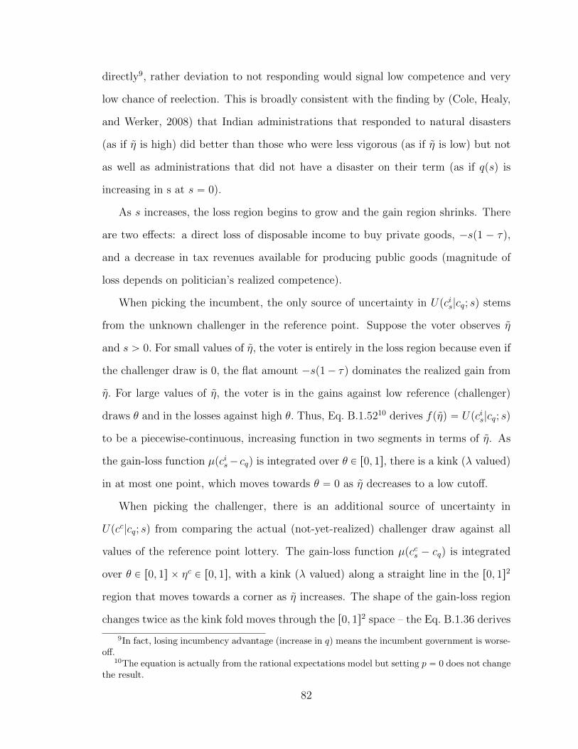
directly9, rather deviation to not responding would signal low competence and very

low chance of reelection. This is broadly consistent with the finding by (Cole, Healy,

and Werker, 2008) that Indian administrations that responded to natural disasters

(as if η is high) did better than those who were less vigorous (as if η is low) but not

as well as administrations that did not have a disaster on their term (as if qpsq is

increasing in s at s “ 0).

As s increases, the loss region begins to grow and the gain region shrinks. There

are two effects: a direct loss of disposable income to buy private goods, ´sp1 ´ τq,

and a decrease in tax revenues available for producing public goods (magnitude of

loss depends on politician’s realized competence).

When picking the incumbent, the only source of uncertainty in Upcis|cq; sq stems

from the unknown challenger in the reference point. Suppose the voter observes η

and s ą 0. For small values of η, the voter is entirely in the loss region because even if

the challenger draw is 0, the flat amount ´sp1´ τq dominates the realized gain from

η. For large values of η, the voter is in the gains against low reference (challenger)

draws θ and in the losses against high θ. Thus, Eq. B.1.5210 derives fpηq “ Upcis|cq; sq

to be a piecewise-continuous, increasing function in two segments in terms of η. As

the gain-loss function µpcis´ cqq is integrated over θ P r0, 1s, there is a kink (λ valued)

in at most one point, which moves towards θ “ 0 as η decreases to a low cutoff.

When picking the challenger, there is an additional source of uncertainty in

Upcc|cq; sq from comparing the actual (not-yet-realized) challenger draw against all

values of the reference point lottery. The gain-loss function µpccs ´ cqq is integrated

over θ P r0, 1s ˆ ηc P r0, 1s, with a kink (λ valued) along a straight line in the r0, 1s2

region that moves towards a corner as η increases. The shape of the gain-loss region

changes twice as the kink fold moves through the r0, 1s2 space – the Eq. B.1.36 derives

9In fact, losing incumbency advantage (increase in q) means the incumbent government is worse-off.

10The equation is actually from the rational expectations model but setting p “ 0 does not changethe result.

82

gpηq “ Upccs|cq; sq to be a piecewise-continuous, decreasing function in three segments

in terms of η.

Therefore, both fpηq “ Upcc|cq; sqpηq and gpηq “ Upcis|cq; sqpηq have analytical

expressions, each is monotonic (See Appendix B for details) and have a unique inter-

section. The optimal cutoff Qpq; sq “ ηqpsq has to be determined numerically11

First, for fixed pα, y, τ, r, k, λq, we get personal equilibrium q˚ in the no-shock

model using qn`1 “ η˚qn iteration. Convergence is fast, about 1 decimal place per

iteration. The fixed point is independent of s and arises as an endogenous reference

point.

Second, for a fixed a grid of s values, for each fixed s find ηpsq that makes the

voter indifferent between candidates, satisfying the piecewise-continuous, algebraic

equation Upcis|cq˚ ; sqpηq “ Upcc|cq˚ ; sqpηq as explained above. This describes how the

optimal decision rule Qpq˚; sq varies with s such that q˚ “ Qpq˚; 0q.

At s “ 0, we have Qpq˚; 0q “ q˚ ă 1{2 by Theorem 3.1 as before, but for s ą 0

incumbency advantage starts to diminish q˚ ă Qpq˚; sq. If also k ą 1, strict convexity

gives incumbency disadvantage in Figures 3.2 and 3.3: for s large enough, Qpq˚; sq ą

12ą q˚.

While this model violates rational expectations for large p, probability of crisis, the

model is a good approximation to rational expectations for small p, when inrepreted

correctly. Although we noted that in the no-shock model, whenever the reference

lottery anticipates elections in a matter inconsistent with the actual decision, given

that lottery, we said that q ‰ η˚q showed the model violated rational expectations.

However, given s ą 0, Qpq˚; sq ­Ñ q˚aspÑ 0.

In the next Sec. 3.4, the rational expectations equilibrium is going to be a pair of

conditional decisions tqnsppq, Qsppqu – how often the voters pick the challenger when

observing no shock and shock, respectively. In the limit as p Ñ 0, we can interpret

11The thresholds for η, where the functional form of each utility function changes, are non-linearlydepend on s, see Figures B.4 and B.2.

83

this Qpq˚; sq “ limpÑ0Qsppq as the probability of picking the challenger when shock of

s magnitude is observed along this sequence of rational-expectation models, with the

observed shock becoming less and less likely. The corresponding q˚ “ limpÑ0 qnsppq

that was derived as the equilibrium of the s “ 0 model would match the probability

of the picking the challenger when the shock is not observed along this sequence of

the rational-expectations models, with the unobserved shock becoming less and less

likely. Therefore, there is no reason to expect these limits to be the same as they are

reached along entirely different sequences.

Figure 3.2 shows, for various curvatures of the gain-loss function, the effect of

increasing negative shocks to future income(%) on incumbency advantage. The values

of the parameters used are as follows: pλ, γ, α, y, τ, rq “ p3, 1, 52, 1, 2

5, 1

10q. For k “

1 incumbency advantage diminishes as the magnitude of catastrophe increases (no

strict convexity in the loss region). For 2 ď k ď 5 (higher curves respectively) risk-

seeing in the losses allows for stronger effect as was predicted and even incumbency

disadvantage (peaking at s “ 0.2y. For large s, qpsq is decreasing towards neutrality

because risk-seeking is predominant for “small” losses and not for “large” losses.

Figure 3.3 is the effect of highr loss-aversion as a sort of limiting guideline. The val-

ues of the parameters used here are as follows: pλ, γ, α, y, τ, rq “ p100, 10, 52, 1, 2

5, 1

10q.

Note that γ2 “ 10 ąą α “ 52ą γ1 “ 1, λ2 “ 100 ąą 3 “ λ1. The effects of losses and

gains has been exaggerated through increase in γ and losses have higher weight than

gains (large λ). For sÑ 0, k “ 1, strong risk-aversion gives large incumbency advan-

tage as q “ 0.352 On the other end of the spectrum, s “ 0.2, k “ 5 gives q “ 0.646 -

a comparable incumbency disadvantage.

84

Figure 3.2: Incumbency (dis)advantage as shock increases for moderate loss-aversion,higher convexity upwards.

Figure 3.3: Incumbency (dis)advantage as the shock increases for high loss-aversion,higher convexity upwards

85

3.4 Rational Expectations of Crisis

Suppose the voter observes whether a negative shock to next period’s income of s

magnitude happens or doesn’t happen before he votes. The shock is a Bernoulli event

with probability p, uncorrelated12 with politician’s ability draw. We will also assume

the challenger’s unobserved ability θ is fixed in secret before the crisis is (un)observed.

The voter’s decision function now depends on pη|sq. Tomorrow’s income is either y or

y ´ s.

When the voter conceives of his reference point for voting, he takes into account

what information he will know at the time13:

1. With probability pQs, there is a crisis and the challenger is elected with unknown

ability θ, which will be reveiled only in period 2,

2. With probability pp1 ´Qsq, there is a crisis and the incumbent is elected with

inferred ability η,

3. With probability p1 ´ pqq, there is no crisis and the challenger is elected with

unknown ability θ,

4. With probability p1´ pqp1´Qsq, there is no crisis and the incumbent is elected

with inferred ability η.

The reference point is a stochastic lottery to the extent it maintains the residual

uncertainty about θ that will remain unresolved in the voting booth when evaluating

next period’s consumption level.

12The shock is an earthquake, change of world price of oil etc, while the ability is personalcompetence of converting private goods into public goods.

13This way the distinction between the incumbent and the challenger remains meaningful. Itwould be pointless to ignore which information will be reveiled in the interim: the incumbent’sability is also unknown when making his reference point and a key tension would be lost. Theincumbent’s decision doesn’t influence the reference-point formation in the model for tractability,and this is why the incumbent moves after the reference point is already formed.

86

Let reference point be

cp “ ppQscθs ` p1´Qsqc

isq ` p1´ pqpqc

θ` p1´ qqciq (3.4.1)

where with probability p the voter will learn there is s shock next period before

voting and with probability 1 ´ p he learns there will be no shock next period. Qs

is the cutoff for incumbent, when the shock happens and q the cutoff when no shock

happens. Here ability θ emphasizes a hypothetical draw of the challenger in the

reference point, giving the corresponding stochastic consumption cθj , j P tns, su. For

more details calculations of the reference consumption in the rational expectations

model, see Sec. B.1. In contrast, when the challenger is elected the actual realization

of his ability is ηc, with a corresponding consumption ccj, j P tns, su. It is critical to

note that just like in the previous section, ηc is different and independent of θ and

the gain-losses are calculated by a double integral over r0, 1s2 in Lemma B.1.

There are two ways to treat the politician’s decision. (i) He observes the shock

before choosing the rent, which means he knows he’ll be losing election with either

q(no shock) or Qs(shock) probability. This is equivalent to the original decision prob-

lem, conditional on the state: public goods vary proportionally to the corresponding

probability of losing. This assumption that the politician can respond to the shock

before choosing his rents in period 1 will be used throughout the rest of the paper.

(ii) He picks rent before he sees the shock. By similar derivation of first-order

conditions, get

g˚1 “ τy ´ r˚1 “ βpR ` rqppQs ` p1´ pqqq (3.4.2)

In this case, the amount of public goods is proportional to the ex-ante expectation

of losing, Erqs “ pQs`p1´pqq. Figure 3.4 shows that Erqs turns out to be relatively

87

Figure 3.4: Ex-ante expected probability of picking the challenger, crisis probabilityp “ 1

3

flat for concave gain-loss function µ because initially for small losses14, q rises with

s at a similar rate as Qs falls with s and the two effects balance out. In this case,

the incumbent maintains an ex-ante advantage, which is reasonable since most in-

cumbents do get reelected. However, in this case the politician cannot respond to the

crisis because he commits to the same decision in both states. The central empirical

analysis, however, looks at variation of disaster relief with respect to the shock, so it

cannot be that the incumbent does not respond.

This model (ii) with k ą 1 does not match the stylized fact of increased government

spending and when k “ 1, it does not match incumbency disadvantage (merely has

decreased advantage) in s. For these reasons, we will assume the incumbent observes

s before choosing rent and public goods at least some of the time as per option (i)

above. As s increases, we find that q falls and Qs rises, so there will be fewer public

goods when a larger shock is averted and more public goods when a larger shock

14The expected loss is increasing in s for k “ 1 with piecewise-linear gain-loss. Incumbencyadvantage remains, though diminished.

88

does happen. Voters’ behavioral utility leads to variation in incumbent’s reelection

chances as S grows and this leads to greater variation in the disaster relief across

states.

The rational-expectations equilibrium is two pairs t`

q, ηpq,Qsq˘

,`

Qs, ηspq,Qsq

˘

u

and satisfies the following 2 conditions:

1. Given any reference point pq,Qsq, in state S the rational decision rule picks

the incumbent pIspη; q,Qsq that equals 1 when Upcis|cpq ě Upccs|cpq and 0

when Upcis|cpq ă Upccs|cpq. In state “not S” the rational decision rule picks

the incumbent pIpη; q,Qsq that equals 1 when Upci|cpq ě Upcc|cpq and 0 when

Upci|cpq ă Upcc|cpq.

2. Fix refence point cp arising from pq0, Q0sq. Given any pair of rational decision

rules derived from cp, the ex-ante rational expectation of challenger losing in

each state is correct:

q0“ Er1´ pIpη; cpqs “ 1´ Pr

´

Upci|cpq ě Upcc|cpq¯

(3.4.3)

Q0s “ Er1´ pI

spη; cpqs “ 1´ Pr

´

Upcis|cpq ě Upccs|cpq¯

(3.4.4)

Moreover, condition (1) above implies a generalization of Theorem 3.1 to show

the existence of a unique pair of decision rules for every reference point cp that is

parametrized by pq,Qsq per Eq. 3.4.1. Each of the unique decision rules is conditional

on the state and maximizes the reference-dependent utility, given the reference point

cp.

Theorem 3.4 (Unique decision pair for each refence point cp). For any reference

point pq,Qsq, there is a unique pair of cutoff decision rules pη˚ns, η˚s q, that depend on

pq,Qsq, so that in each state j P ts, nsu, η˚j : r0, 1sˆr0, 1s Ñ p0, 1q defines the following

89

optimal voting rule as:

pIjpη; q,Qsq “

$

’

’

&

’

’

%

1 if η ě η˚j ,

0 if η ă η˚j .

Proof outline. 1. Fix state j P ts, nsu and define fjpηq “ Upcij|cpq. Use the explicit

formulation in Appendix 1 to show that f is strictly increasing in η. Apply the proof

of Lemma B.6 piecewise for each of the two segments in terms of η with cutoff H ijpsq,

that only depends on parameters other than η. Intuitively, the direct utility of picking

an incumbent rises faster in his ability than a reference point that has a pjp1 ´ qjq

weight on η.

2. Define gjpηq “ Upccj|cpq. Use the explicit formulation in Appendix 1 to show

that g is weakly decreasing in η. Apply the proof of Lemma B.5 piecewise for each

of the three segments in terms of η with cutoffs H ijpsq and H

i

jpsq. These cutoffs only

depend on parameters other than η. Intuitively, the utility of picking a challenger falls

in the incumbent’s ability as the reference point rises with pjp1´ qjq weight on η.

3. pfj ´ gjqp1q ą 0 and pfj ´ gjqp0q ă 0. Each state fixes the after-tax income

for consumption of the private good, but consumer’s choice affects the variation of

the public goods next period (pinned-down by politician’s ability). Selecting the best

incumbent of highest ability 1 is strictly preferred to pulling an unknown challenger

and the worst incumbent is strictly worse than a random challenger draw, for any

reference point cp.

4. Then fj ´ gj has a unique root on p0, 1q by IVT. Denote this root as η˚j . This

is the unique value solves Upcij|cp; η˚j q “ Upccj|cp; η

˚j q. It is the interior threshold in

state j P ts, nsu when the citizen is indifferent between a random challenger and an

incumbent of known ability η˚j , while the reference point is fixed at pq,Qsq.

90

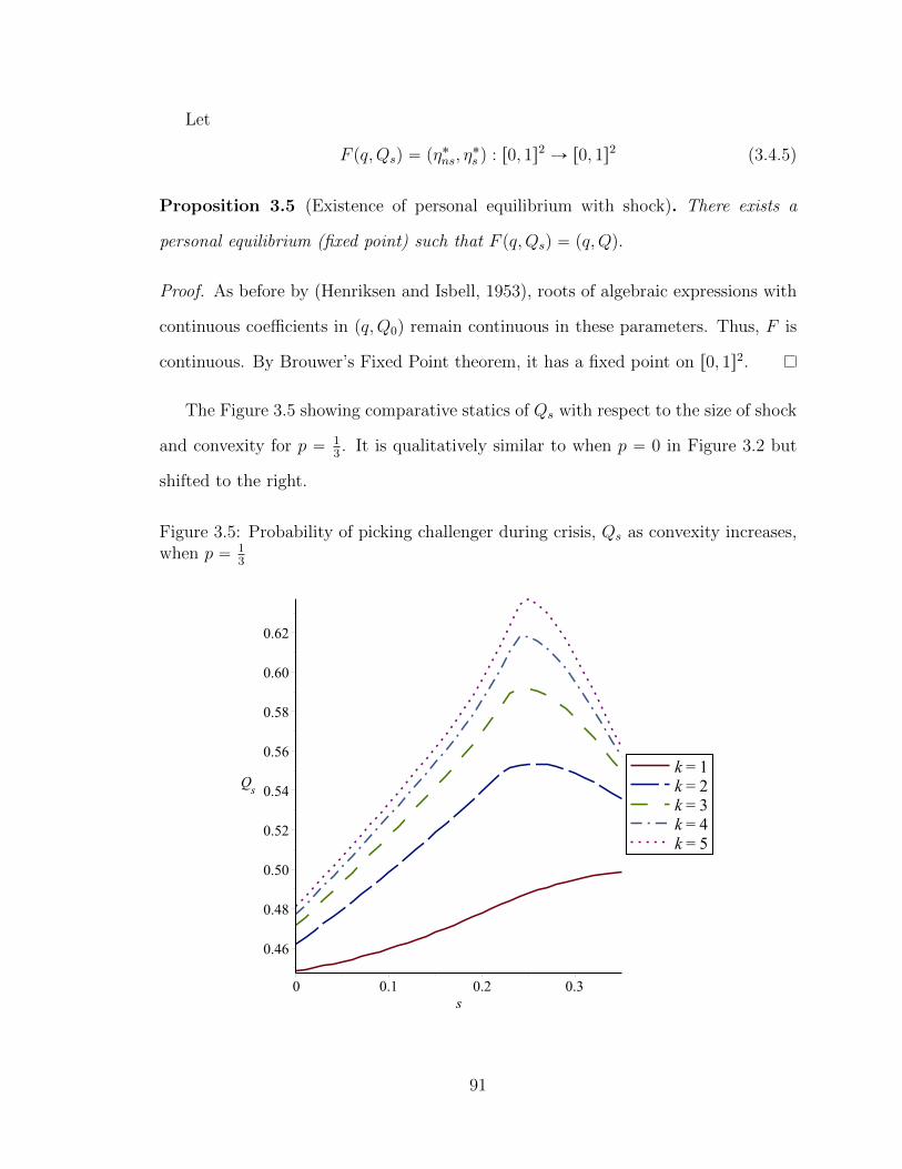
Let

F pq,Qsq “ pη˚ns, η

˚s q : r0, 1s2 Ñ r0, 1s2 (3.4.5)

Proposition 3.5 (Existence of personal equilibrium with shock). There exists a

personal equilibrium (fixed point) such that F pq,Qsq “ pq,Qq.

Proof. As before by (Henriksen and Isbell, 1953), roots of algebraic expressions with

continuous coefficients in pq,Q0q remain continuous in these parameters. Thus, F is

continuous. By Brouwer’s Fixed Point theorem, it has a fixed point on r0, 1s2.

The Figure 3.5 showing comparative statics of Qs with respect to the size of shock

and convexity for p “ 13. It is qualitatively similar to when p “ 0 in Figure 3.2 but

shifted to the right.

Figure 3.5: Probability of picking challenger during crisis, Qs as convexity increases,when p “ 1

3

91

In Figure 3.6, we can see that conditional on the shock, there is increase in in-

cumbency disadvantage but conditional on no shock, there is increase in incumbency

advantage. The first result shows that this finding in the ad hoc model was robust.

The second result is new information that wasn’t available in the ad hoc model. The

interpretation is as follows: the voter is pleasantly surprised to find himself in the gains

relative to the reference point that was putting positive weight on the shock. In the

gains, gain-loss function generates risk-aversion, so the incumbent gets reelected more

often. Thus, the presence of the shock event makes incumbency advantage stronger,

so the conditional change from q to Qs is greater under rational expectations of shock

than in the “surprise” model.

Figure 3.6: Conditional probabilities of picking the challenger pq,Qsq, p “13, k “ 5

92

In the previous section we’ve used an ad hoc model of “surprise” shock. It was

unreasonable in the sense that voters were sophisticated enough to calculate q˚ as a

rational expectations equilibrium in the no-shock model but were not sophisticated

enough to account for the true probability p of the shock. In particular, the incum-

bency disadvantage was not rationally anticipated, ever.

The purpose of that model was of convenience – it used existence results for the

simpler no-shock model and that simpler model only needed to be solved once for

the fixed point. Then taking that fixed point, the decision rule as a function of s

was a sequence of roots of piecewise-continuous expressions of utility differences in η.

Qualitatively, the ad hoc model was successful in that it verified stylized facts from the

empirical literature about incumbency advantage switching to disadvantage during

crisis and about the incumbent increasing public goods expenditure with shock, while

losing more often.

The full-blown rational expectations model is a robustness check. Numerical cal-

culations show that the stylized results still hold even for arbitrary 0 ă p ă 1, though

the calculations become more intensive. After fixing the other parameters, except

for the shock magnitude s, the RE model is solved for a fixed-point pair pq,Qsq for

each s on a grid as follows. Taking an arbitrary pair pq0, Q0sq and the corresponding

c0p with those weights, we solve for the optimal decision rule in each state, given c0

p.

Then the new pair pq1, Q1sq corresponds to c1

p and the process is re-iterate to get the

new decision pair etc, until convergence is attained to arbitrary precision. The con-

vergence is still fast, on the order of 1 decimal place per iteration for any starting

condition. This iterative process is then repeated for each value of s on a grid, to get

a grid of fixed points ts, pq,Qsqu. In contrast, in the ad hoc model there was only one

calculation per s because the refence point q˚ was iterated only for s “ 0 and then

reused.

93

The following Proposion 3.6 is an analytic result that leverages continuity and

monotonicity of the algebraic functional forms for utility functions from Sec.B to

get continuity of the resulting fixed points. This Proposition highlights the general

connections between the fixed-point maps of the rational expectations and the ad hoc

models.

Proposition 3.6 (Surprise model as a limit under RE). Take the personal equilibrium

q0 from the no-shock model and the corresponding decision rule Qpq0;Sq as a function

of shock S in the “surprise model,” satisfying q0 “ Qpq0; 0q. Now fix p and pick a

personal equilibrium pair pq,Qsq for each S in the rational-expectations model with the

corresponding decision-pair map F px, y;S, pq “ pF nspx, y;S, pq, F spx, y;S, pqq, whose

components depend on S and p, satisfying F pq,Qs;S, pq “ pq,Qsq.

Then

F nspa, a; 0, pq “ F s

pa, a; 0, pq “ Qpa; 0q “ a equality along S “ 0 (3.4.6)

F nspb, B;S, 0q “ Qpb; 0q “ b equality along p “ 0 (3.4.7)

F spd,D;S, 0q “ Qpd;Sq equality along p “ 0 (3.4.8)

Proof. By previous Theorems 3.1 and 3.4, all decision rules are continuous in param-

eters (because the utilities are and gain-loss functions are, from which the decision

rules are derived as roots of algebraic expressions). Thus, the decision rule in the

limit model equals to the limit of the decision rules.

Recall that,

cp “ ppQscθs ` p1´Qsqc

isq ` p1´ pqpqc

θ` p1´ qqciq (3.4.9)

cq “ qcθ ` p1´ qqci (3.4.10)

94

1. When s “ 0, we have

cp “ cθ`

pQs ` p1´ pqq˘

` ci`

pp1´Qsq ` p1´ pqp1´ qq˘

If also Qs “ q “ a, then cp “ cq. The rational expectations reference point of

0 shock with probability p is equal to the no-shock reference point by construction,

whenever q “ QS, which are both equal to a here. Thus, the RE decision in the

shock state with S “ 0, given the same reference point, coincides with the ad hoc

decision when S “ 0: F spa, a; 0, pq “ Qpa; 0q. The decision rule in the model without

shocks is the same as the decision rule in the RE model of shock s Ñ 0 along the

q “ Qs path. When s “ 0, moreover, the utilities of the RE model are equal in each

state for arbitrary reference-point pair: Upcc|cp;S “ 0, pq “ Upccs|cp;S “ 0, pq and

Upci|cp;S “ 0, pq “ Upcis|cp;S “ 0, pq Thus, the corresponding decisions are equal in

each state: F nspq1, Q1; 0, pq “ F spq1, Q1; 0, pq and take q1 “ Q1 “ a.

2. When p “ 0, we have an identity for the reference points in the RE and the ad

hoc models, independent of Qs,

cp “ bcθ ` p1´ bqci “ cb

Conditional on observing no shock, when shocks occurs with p “ 0 the decision is the

same as being always surprised by observing a shock of S “ 0, when not anticipating

any shock, F nspb, B;S, 0q “ Qpb; 0q because utilities coincide as Upcc|cp; p “ 0q “

Upccs|cb;S “ 0q and Upci|cp; p “ 0q “ Upcis|cb;S “ 0q.

3. When p “ 0, then cd “ cppd,Qs; p “ 0q for any Qs as above. The utilities

in the “surprise” model are equal to the rational expectations utilities when the

shock is observed under reference point cd : Upccs|cp;S, p “ 0q “ Upccs|cd;Sq and

Upcis|cp;S, p “ 0q “ Upcis|cd;Sq. Equivalently, the reference point is cp restricted to

95

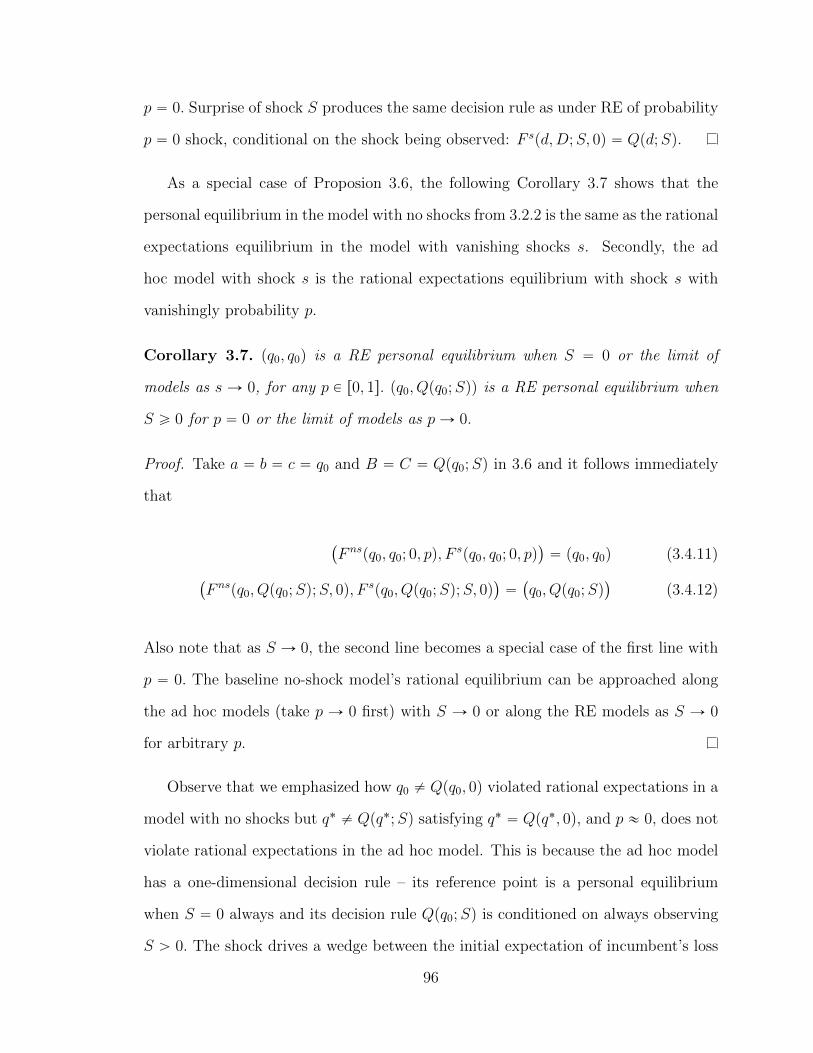
p “ 0. Surprise of shock S produces the same decision rule as under RE of probability

p “ 0 shock, conditional on the shock being observed: F spd,D;S, 0q “ Qpd;Sq.

As a special case of Proposion 3.6, the following Corollary 3.7 shows that the

personal equilibrium in the model with no shocks from 3.2.2 is the same as the rational

expectations equilibrium in the model with vanishing shocks s. Secondly, the ad

hoc model with shock s is the rational expectations equilibrium with shock s with

vanishingly probability p.

Corollary 3.7. pq0, q0q is a RE personal equilibrium when S “ 0 or the limit of

models as s Ñ 0, for any p P r0, 1s. pq0, Qpq0;Sqq is a RE personal equilibrium when

S ě 0 for p “ 0 or the limit of models as pÑ 0.

Proof. Take a “ b “ c “ q0 and B “ C “ Qpq0;Sq in 3.6 and it follows immediately

that

`

F nspq0, q0; 0, pq, F s

pq0, q0; 0, pq˘

“ pq0, q0q (3.4.11)

`

F nspq0, Qpq0;Sq;S, 0q, F s

pq0, Qpq0;Sq;S, 0q˘

“`

q0, Qpq0;Sq˘

(3.4.12)

Also note that as S Ñ 0, the second line becomes a special case of the first line with

p “ 0. The baseline no-shock model’s rational equilibrium can be approached along

the ad hoc models (take p Ñ 0 first) with S Ñ 0 or along the RE models as S Ñ 0

for arbitrary p.

Observe that we emphasized how q0 ‰ Qpq0, 0q violated rational expectations in a

model with no shocks but q˚ ‰ Qpq˚;Sq satisfying q˚ “ Qpq˚, 0q, and p « 0, does not

violate rational expectations in the ad hoc model. This is because the ad hoc model

has a one-dimensional decision rule – its reference point is a personal equilibrium

when S “ 0 always and its decision rule Qpq0;Sq is conditioned on always observing

S ą 0. The shock drives a wedge between the initial expectation of incumbent’s loss

96

(q less than 12) and the actual (Qpq;Sq ą 1

2for moderate s). But taking the personal

equilibrium from the rational expectations model, the fixed-point is now with respect

to a different map F with two components that evaluates this wedge correctly and

parametrized by p “ 0: F pq0, Qpq0;Sq;S, 0q “ pq0, Qpq0;Sqq.

3.5 Conclusion

This paper takes a new look at the studied problem of incumbency advantage using

behavioral loss-averse, reference-dependent preferences to explain recent behavioral-

like empirical findings. Personal equilibrium of Koszegi and Rabin (2007) is applied

to voters who rationally expect their own reference point formed by their future

rational voting decision. This gives analytical precision to the suggestive intuition

found in Quattrone and Tversky (1988). The explanation does not depend on specific

features of legislature politics and can be applied to explain the pervasive incumbency

advantage found in any kind of elections (state and federal legislatures, gubernatorial

and state executives) as Ansolabehere and Snyder Jr (2002) has found. Wolfers (2007)

and Achen and Bartels (2004) both find that challengers do better in bad times

after an exogenous shock (economic and natural shocks, respectively), unrelated to

the government’s actions, and incumbents during normal/good times is consistent

with qpsq increasing in s for small s. These authors suspect some sort of behavioral

mechanism but do not construct one. Reference-dependent risk preferences offer just

such a mechanism.

A model that only has politicians with career concerns and rational voters will have

the incumbent exert some effort in the first period as well but because his probability

of winning wont be related to irrelevant signals (exogenous shock to income), he won’t

alter the public goods spending as the shock varies. In fact, γ “ 0 gives q “ Qs “12

97

for all parameter values – judging politicians solely on their innate talent makes

incumbents and challengers interchangeable ex-ante.

This paper finds that the analytical incumbency advantage requires only a feasi-

ble reference point, which need not be endogenous, and a weakly concave gain-loss

function. To generate incumbency disadvantage (numerically) and the corresponding

disaster relief through the “career-concerns” channel, the endogeneous reference point

is used as a selection device to make the model’s prediction tighter for the purposes

of the comparative statics as s increases. Incumbency disadvantage is first illustrated

in a simpler ad hoc model with where the voters are surprise by anticipated crisis

that always happens. Then, that model is nested within a consistent rational ex-

pectations model where crisis happens with known probability p, which enters (and

complicates) the reference point of a voter. Finally, a limiting continuty argument

connects all three models together.

Cole, Healy, and Werker (2008)’s finding about electoral performance of Indian

administrations during terms with and without earthquakes is consistent with the

story of politicians showing their competence ηi (or lack-of-thereof) through govern-

ment responses (public good provision, g1pqq, yet doing worse-off ex-post: both value

function of the incumbent vIpqq and probability of winning pI decrease when incum-

bency advantage falls at the same time as rents r1pqq fall and public outlays increase

g˚1 pqq.

Another avenue for loss aversion would be politicians’ preferences. A challenger

may be unwilling to fight as hard to gain the position in question, compared to

incumbent determined to avoid losing. This could explain the powerful deterrence

phenomenon where a fraction of incumbent house races goes uncontested (Diermeier,

Keane, and Merlo, 2005; Stone, Maisel, and Maestas, 2004). If this was one important

reason for deterrence of entry and if deterrence was causing the upward trend for

incumbency advantage, it is unclear why effects of loss aversion would increase over

98

time. Reference-dependent preferences may give reasonable explanation for cross-

sectional data but less plausible to explain temporal drift found by Gelman and King

(1990).

99

Chapter 4

Fault-Tolerant Bayesian

Implementation in General

Environments

Classical implementation theory uses Nash equilibrium as its solution concept, which

assumes that each agent is fully rational and can choose his most preferred strategy.

In this case, player i expects all other players will follow their equilibrium strategy.

If some other players deviated by a mistake, then i may want to deviate as well.

The concept of fault-tolerant implementation was introduced by Eliaz (2002) for

environments of complete information. The idea is to consider a stronger equilibrium

notion than Nash equilibrium, so that players have no incentive to deviate from the

equilibrium strategy for any private belief about the identity and behavior of up to

k faulty players. Perhaps, a minority of players are making mistakes, malicious, be-

havioral or did not understand instructions. The 0-fault-tolerant equilibrium reduces

to Nash equilibrium and pN ´ 1q-fault-tolerant equilibrium is weak dominance.

100

A stronger statement of full implementation1 for social choice correspondences in-

cludes a new requirement that all k-deviations from k-FTNE equilibria are desirable.

This is because even when all rational players adhere to their equilibrium strategies,

the outcome of the mechanism may change because of deviations by k faulty play-

ers. In some sense, these k-deviations near the equilibrium come bundled with the

equilibrium. Since we want each equilibrium to be desirable, it is reasonable that the

bundle of k-deviations is also desirable.

Eliaz (2002) showed that k-monotonicity2 of the social-choice correspondence and

standard no-veto power3 are sufficient for full implementation. Furthermore, weak

k-monotonicity is necessary for full implementation.

The current paper extends fault-tolerant implementation from Eliaz (2002)’s com-

plete information setting to an incomplete information setting, similar to Jackson

(1991). Here, agents have private information about the state of the world and ex-

clusive4 information is allowed. Exclusive information is relevant for the study of

auctions, public goods provision, delegation games, partnership arrangements, etc.

There is no objective measure of faultiness that is revealed to the social planner or

any of the players. It is a key assumption that players are allowed to have arbitrary

specific beliefs5 about who (if any) is faulty and what state-dependent strategy they

play. These beliefs are degenerate lotteries as there is no uncertainty about faultiness

for any fixed belief. A different analysis may allow for subjective and arbitrary non-

degenerate lotteries over faultiness of others.

1Every equilibrium of a mechanism is desirable and every desirable outcome can be supportedby an equilibrium.

2Reduces to Maskin monotonicity for k “ 03No single player can be a dictator in the senes that if everyone but that player find an outcome

most preferred, it must be desirable in the social choice set.4Non-exclusive information means any N´1, or possibly any N´k´1, players collectively have

complete information.5But even under the most favorable beliefs, there is no profitable deviation for any non-faulty

player as long as upper bound of k is not violated.

101

Similar to Jackson (1991), the environment in the current paper is a general one.

It is not necessarily economic6, best and worst allocations across all states sometimes

may not exist and full support is relaxed.

Figure 4.1: Relevant Literature on Implementation

MaskinvDN977Z

PostlewaitevandSchmeidlervDN986Z

EliazvDpTTpZ

Ge

ne

ral

En

viro

nm

en

tE

xcha

nge

Exc

hang

eG

ener

alG

ener

al

PalfreyvandvSrivastavavDN989Z

JacksonvDN99NZ IaralovvDpTN3Z

DoghmivandZiadvDpTT7Z

ClassicalvEquilibrium kbFaultvTolerantvEquilibrium

No

nb

Exclu

siv

eE

xclu

sive

Com

plet

e

Robust to k faults

Inco

mp

lete

In

form

atio

n

There are different ways we can model faulty players under incomplete information

and it ties-in to the choice of the equilibrium and implementation concepts. For

example, allowing only pure or also mixed strategies, assuming players have some

specific or arbitrary beliefs about the faultiness of others, requiring (or not) that k-

deviations from the equilibrium need to be desirable. Consider combining exclusive

information setting with faulty players in the way that reproduces the approach from

6An economic environment has at least two players that aren’t satiated at any social choicefunction and each prefers some other social choice function. An exchange economy with N ě

3 players is an economic environment because there are always 2 players who don’t get the fullendowment. For an example of a non-economic environment consider an economy where in somestate everyone is indifferent between every feasible social choice function.

102

Eliaz (2002) with a single state when each player has exactly one type and reproduces

the approach from Jackson (1991) when no faulty players are allowed (k “ 0). Even

this straightforward extension develops some novel difficulties.

Non-exclusive information settings, such as complete information structure, are

not sensitive to deceptions by a minority because the correct state can be correctly

inferred if the majority is truthful. This covers both a rational agent considering

a unilateral deception and a group of faulty players deceiving by a mistake. The

exclusive information setting means that individual players’ reports of their state are

unverifiable and the mechanism takes them at face value. The incentive compatibility

condition keeps rational agents honest when everyone else is truthful. The added

complication is in considering deceptions by a minority of faulty players because

they are not constrained by incentives and their reports are unverifiable. Therefore,

the mechanism cannot decipher the types of faulty players directly in an exclusive

information setting.

The equilibrium requirement has N´k players continuing to play their prescribed

strategies, even when k players deviate. To get partial implementation, the incentive

compatibility condition is strengthened to be insensitive to deceptions that are in the

k-ball around the truth. That is, as long as the other N ´ k ´ 1 players are truthful,

the individual player i prefers to tell the truth. This sustains any desirable outcomes

as an equilibrium.

The second complication arises when going in the other direction to get full im-

plementation. The mechanism and a monotonicity condition work together to ensure

deceptions of the majority7 that lead to undesirable outcomes are broken up by a

“whistleblowing” minority. The mechanism designer is concerned that a malicious

minority may deviate to break a desirable equilibrium when no deception is taking

place. The key ingredient of the mechanism is to block any minority objection that

7Incentive compatibility doesn’t apply when other players are not truthful.

103

is preferred for some type of some player in the minority when no deception is taking

place and the majority proposes some x that is desirable. Similarly, the key ingredient

of the monotonicity condition is, for each non-desirable majority deception, generat-

ing a state s and an objection y less preferable than x for “whistleblowers” when

the majority is truthful, for all types of the objecting players, while preferring the

objection in that specific state only if the majority is deceptive.

This second complication is that a minority of k ` 1 players under exclusive in-

formation setting have different information sets. In Jackson (1991), the objecting

minority consists of exactly one player and his information set is trivially constant

across the minority (equal to itself). In Eliaz (2002), the objecting minority consists

of k ` 1 players but their information set is the same singleton because information

is complete. If the information set is common8, then the faulty players’ types are

constant along the rational player’s information set. Thus, the faulty players have a

constant message under arbitrary deceptions along the rational player’s information

set. Since the planner doesn’t block the faulty players’ message at s (by construction),

he doesn’t block their message at all states in rational player j’s information set. This

was the case in the previous literature – in Doghmi and Ziad (2007) faulty deceptions

did not matter because the planner knew the true state in every k´deviation of every

equilibrium and the special structure of the environment allowed punishments to stay

within a single rule of the mechanism.

On the other hand, when the faulty players’ types may vary across the rational

player j’s information set, the mechanism will allow the “whistleblowing” coalition

to replace x with y on a neighborhood of a true state s and potentially block it on a

disjoint subset of the rational player j’s information set at sj. This block is to prevent

potential “conflict of interest” by one of the coalition members, had they been rational

and had a type that strictly preferred y to x when the majority was, in fact, truthful.

8As Observation 4.10 in Section 4.2 notes, it is enough that the rational player’s information setis weakly coarser than the common intersection of the coalition’s information sets.

104

The condition k-monotonicity-no-veto (k-MNV) has to track these subsets when it is

describing the outcomes of the mechanism for j’s deviation and non-deviation along

his information set at sj, so that j is ready to form a k`1 minority coalition to break

the equilibria with non-desirable outcome when a majority coalition asks for x with

a majority deception.

This paper defines a central condition called k-incentive compatibility (k-IC), a

direct generalization from Jackson (1991)’s incentive compatibility. k-IC is both nec-

essary and sufficient for partial implementation9 in k-FTBE of social choice sets that

satisfy closure. The usual incentive compatibility requires that whenever everyone

is telling the truth, the agent also prefers to tell the truth about his type, for any

type realization. This condition is important because under exclusive information

the planner has to rely on each agent to report their private state to determine the

appropriate allocation. On the other hand, under non-exclusive information (includ-

ing symmetric complete information), the planner can rely on a consensus of reports,

so he doesn’t have to rely on individual person’s report. Secondly, the planner can

enforce consensus by punishing obvious deviators who report information that is in-

consistent with the consensus. The complication of k faulty players under exclusive

information allows for “hidden” lies. Even when the correct social choice function

is picked, a given player is allowed to have arbitrary beliefs about k faulty players

lying about their type. When the social choice set satisfies k-IC, as long as the other

N´k´1 players tell the truth, this given player finds it optimal to also tell the truth.

When the social choice set also satisfies k-monotonicity-no-veto10, full implemen-

tation in k-FTBE is achieved. The downside is that k-MNV is a fairly complicated

statement that generalizes Jackson (1991)’s MNV to k faulty players. Originally,

MNV was a combination of no-veto power and Bayesian monotonicity where in some

9For any desirable social choice function, there is an equilibrium whose outcome agrees with thefunction.

10k-MNV combines k-no-veto-hypothesis and k-Bayesian monotonicity

105

states no-veto-hypothesis is satisfied11 and in other states, Bayesian monotonicity

generates a profitable deviation to kill equilibria with non-desirable outcomes. The

states when NVH holds are precisely the states when the integer game is played

and outcomes in those states are indifferent (else someone could deviate their integer

strategy to win a better outcome for those states). Under symmetric information in

Eliaz (2002), the information set is a singleton and either the integer game is played

in equilibrium or not. In contrast, in a Bayesian equilibrium with incomplete in-

formation, on a subset of the information set, some states lead to the integer game

and for other subsets the integer game is not played. This means the constructed

deviation is more involved under incomplete information as it has to identify what

outcomes result from different rules of the mechanism under different subsets of a

given information set.

In Jackson (1991), monotonicity-no-veto gives the second condition of full imple-

mentation: for each equilibrium, there is a social choice function that matches that

equilibrium’s outcome. Here, k-MNV goes further and considers the whole ball of

k-deviation around each equilibrium and finds a desirable function for each element

in the ball.12

Weak k-Bayesian monotonicity is necessary for full implementation. When players

try to play a deception that leads to a non-desirable outcome by manipulating their

reports of the state, full implementation cannot admit such an equilibrium and so

it generates a group of k ` 1 “whistleblowers.” They offer a minority objection as

a deviation that is less preferable under the truth for each player, relative to some

11When N ´ 1 players reach a consensus and the N -th player does something else, he cannottrigger the integer game alone. However, any of the N ´ 1 players, when deviating, may triggerthe integer game and win any prize. Since they don’t find it profitable to break equilibrium inthose situations, they must prefer the equilibrium outcome to anything else they could’ve asked for.Perhaps, there are many ties in that state. No-veto hypothesis maintains the desirability of theequilibrium because N ´ 1 players find it most preferred.

12Any equilibrium with a non-desirable k-deviation is eliminated by construction in k-MNV.

106

other desirable outcome13. Moreover, this objection is strictly better under the pro-

posed deception for one of the “whistleblowers,” who finds it a profitable deviation

under the belief that the other k “whistleblowers” are faulty and play the speci-

fied minority objection. Doghmi and Ziad (2007) have a corresponding result for

an exchange economy, restricting attention to compatible deceptions14. In general

economies, the statement is a bit stronger by not requiring compatible deceptions.

Using the special structure of an exchange economy, their mechanism punishes every-

one for non-compatible deceptions by giving everyone the 0 allocation, which is the

worst outcome for all states. Since more general environments need not have such an

outcome, non-compatible deceptions are also allowed.

In the previous work of Doghmi and Ziad (2007), they extended k-fault imple-

mentation to incomplete information in a more specific environment: an exchange

economy with non-exclusive information as in Palfrey and Srivastava (1989). Doghmi

and Ziad (2007) use k-non-exclusive information, which becomes more restrictive as

k increases because the smaller remaining group knows everything. While allow-

ing robust implementation despite the presence of faulty players, the informational

requirement becomes more restrictive and takes a step back towards symmetric infor-

mation. More recently, Doghmi and Ziad (2009) re-examines k-FTNE implementation

of social-choice correspondences in exchange economies with complete information.

In some specific environments (e.g. single-peaked preferences with unanimity), their

strict k-monotonicity is a sufficient condition for full implementation because the set-

ting provides a weak form of NVP “for free.” In other words, this line of work on

robust implementation is trying to tighten the gap between sufficient and necessary

conditions in Eliaz (2002) by weakening or dropping the no-veto-power. This setting

13It is a weak k-BM because this preferred outcome can be different for each member of thegroup.

14Compatible refers to deceptions satisfying s P T implies αpsq P T, where T is the set of statesoccurring with non-zero probability.

107

also does not allow for exclusive information or environments more general than an

exchange economy.

Doghmi and Ziad (2007) find that when a social choice set satisfies k-Bayesian

monotonicity and assuming non-exclusive information (roughly, every group of at least

k players collectively pins down the state of nature to a singleton), full implementation

is achieved. The corresponding necessary condition is weak k-Bayesian monotonicity.

The authors observe that Bayesian monotonicity neither implies nor is implied by

weak k-Bayesian monotonicity under incomplete information, similar to the result in

Eliaz (2002) that weak k-monotonicity is distinct from Maskin monotonicity.

An exchange economy is a special case of an economic environment, has a worst

and a best element independent of the state15, which allows to restrict attention only

to compatible deceptions. The social planner observing non-compatible deception

knows that someone has deviated, not necessarily whom. Mechanisms in exchange

economies following Palfrey and Srivastava (1989) give collective punishment of 0 to

everyone in such cases to rule them out. They also assume full support and that there

is an objective conditional distribution of faultiness over players that is independent

of state realization. The special environment structure implies a special result is

used to prove sufficiency of k-Bayesian monotonicity and k-non-exclusive information

to achieve full implementation. The result states that in all states, the equilibrium

outcomes come from the first rule of their mechanism: at least N ´ k non-faulty

players agree on the state, agree on the allocation rule and don’t initiate the integer

game.

An exchange economy is unlike a more general environment that allows outcomes

of equilibria to satisfy NVH for the subset of the information set where the integer

game is played. In contrast, there are equilibria in general environments that trigger

multiple rules of the mechanism across an information set of some fixed player’s

15In any state, receiving the full endowment E is ideal. In any state, receiving 0 endowment isthe worst outcome.

108

type because players with exclusive information find it harder to coordinate: on a

subset of his information set others coordinate on the same desirable x, on a disjoint

subset others coordinate on some other x, on another disjoint subset coordination fails

and the integer game rule is triggered but they cannot improve on the equilibrium

outcome.

4.1 Environment

Notation and definitions are borrowed or adapted from Jackson (1991), Eliaz (2002),

Saglam (2007), and Doghmi and Ziad (2007).

An environment is a collection of tN,S,A, tqipsqu, tU iuu : N is the finite number

of players16; S is the set of states describing agents’ information and preference:

s “ ps1, ¨ ¨ ¨ , sNq P S, where |Si| is finite; A is the set of feasible allocations or

consequences, fixed across states; qi is the prior of agent i on S; U i : A ˆ S Ñ R`

is the state-dependent utility function. The set of all social choice functions is X “

tx|x : S Ñ Au.

Agents agree on which states occur with positive probability: whenever qipsq ą 0

then qjpsq ą 0 for all j ‰ i. The common support of their priors is denoted by

T “ ts P S|qipsq ą 0u, which is equal for all i. The priors qi define partitions of T ,

Πi, with elements referenced by πi. For a given information signal (type) si P Si, let

πipsiq “ tt P S|ti “ si and qiptq ą 0u P Πi

be the plausible true states given agent i’s information. Without loss of generality,

each type has a non-empty information set: @i P N, @si P Si, πipsiq ‰ H. Agents’

16With slight abuse of notation, N will subsequently refer to both the set of all players and thecardinality of that set.

109

preferences (complete and transitive) over social choice functions have a conditional

expected utility representation. For fixed x, y P X, si P Si,

xRipsiqy ðñ

ÿ

sPπipsiq

qipsqU irxpsq, ss ě

ÿ

sPπipsiq

qipsqU irypsq, ss

A social choice set F Ă X is a collection of “desirable” social choice functions.

Out of N players, at most k players are faulty who do not act according to

incentives. Non-faulty players know they are not faulty but do not know who (if any)

faulty players are, except that there are between 0 and k (inclusive) faulty players.

A mechanism consists of an action space M “ M1 ˆ ¨ ¨ ¨ ˆMN and a func-

tion g : M Ñ A. A (pure) strategy for i is a map from information sets to mes-

sages, σi : Si Ñ Mi. Denote vector of strategies σ “ pσ1, ¨ ¨ ¨ , σNq; pσ´i, τ iq “

pσ1, ¨ ¨ ¨ , σi´1, τ i, σi`1, ¨ ¨ ¨ , σNq. The outcome social choice function of σ is xpsq “

gpσpsqq.

4.2 Definitions

By relaxing the full-support assumption, the objects of interest are the outcomes of

social choice functions along the (plausible) states of non-zero measure.

Definition 4.1. The social choice functions x and y are equivalent if @s P T, xpsq “

ypsq. The social choice sets F and F are equivalent if @x P F, Dx P F which is

equivalent to x, and @x P F , Dx P F which is equivalent to x.�

The following notation of splicing will be useful to give meaning to one social

choice function z being preferred to z over a subset of states C, e.g. zRjpsjqz{Cz.

Definition 4.2. Let x{Cz be a splicing of two social choice functions x and z along

a set C Ă S. The social choice function x{Cz is defined as @s P C, rx{Czspsq “ xpsq

and rx{Czspsq “ zpsq otherwise.�

110

When the social planner faces incomplete and exclusive information, he relies

on citizen’s incentives to report their type as he has no other way of learning the

aggregate state, which is simply a collection of realized types of players. When citizens

try to cheat by asking for a desirable social choice function x P F but manipulate

their reporting to get wrong allocations in various states, we say they are playing

a deception x ˝ α. When this deception leads to a non-desirable outcome, a form of

Bayesian monotonicity will be later used to eliminate the underlying equilibrium with

deception α.

Definition 4.3. A deception for i P N is a mapping αi : Si Ñ Si. Let Ai “ tαi|αi :

Si Ñ Siu be the set of all deceptions of player i, A “ A1 ˆ A2 ¨ ¨ ¨ ˆ AN and A´i are

defined accordingly. Let α “ pα1, ¨ ¨ ¨ , αNq P A and αpsq “ rα1ps1q, ¨ ¨ ¨ , αNpsNqs. The

notation x ˝ α represents the social-choice function, which results in xrαpsqs for each

s P S.�

Jackson (1991) points out that closure is a basic requirement for implementation

of social choice sets. Suppose that the common knowledge concatenation Π has two

elements. Pick any two equilibrium strategies of a specific mechanism. Construct a

third strategy as follows: players use the first strategy on the first element of Π and

the second strategy on the second element of Π, must also be an equilibrium of the

mechanism (otherwise, any deviation against the third option would eliminate one of

the two original equilibria, based on which element of Π the deviation was in). By

full implementation, the outcome of the third equilibrium is desirable.

Definition 4.4 (Closure). Let B and D be any disjoint sets of states such that

B Y D “ T and @π P Π, either π Ă B or π Ă D. A social choice set F satisfies

closure (C) if @x, y P F, Dz P F s.t. @s P B, zpsq “ xpsq and @s P D, zpsq “ ypsq.�

The stronger notion of full implementation requires that any outcome in a k-ball

of an equilibrium to be desirable. Likewise, beliefs about arbitrary “hidden lies” can

111

be translated into a k-ball of deceptions around the non-faulty deception α (or the

identity map, id, when planning to tell the truth).

Definition 4.5 (k-neighborhood). Given vector profile v˚ P V and an upper bound

for faulty players k, Bpv˚, k;V q “ tv P V : |ti P N : v˚i ‰ viu| ď ku is a k-

neighborhood of v˚ (with respect to V), is the set of profiles that are different from v˚

by not more than k entries.�

The complication of k faulty players under exclusive information allows for “hid-

den” lies. Even when the correct social choice function is picked, a given player is

allowed to have arbitrary beliefs about k faulty players lying about their type. When

the social choice set satisfies k-IC, whenever the other N´k´1 players tell the truth,

this given player finds it optimal to tell the truth also.

Definition 4.6 (k-IC). Given i P N, define id : S Ñ S to be the identity map and

β´i P Bpid, k;A´iq is a profile of deceptions for players Nztiu in the k-neighborhood

of the truth. A social choice set F satisfies k-incentive compatibility (k-IC) if

@x P F, @i P N, @β´i P Bpid, k;A´iq, @ti, si P Si, x ˝ pβ´i, idqRi

psiqx ˝ pβ´i, tiq.�

When players try to play a deception that leads to a non-desirable outcome by

manipulating their reports of the state, full implementation cannot admit such an

equilibrium and so it generates a group of k`1 “whistleblowers.” They offer a minority

objection as a deviation that is less preferable under the truth for each player, relative

to some other desirable outcome. It is a weak k-BM because this preferred outcome

can be different for each member of the group. Moreover, this objection is strictly

better under the proposed deception for one of the “whistleblowers,” j, who finds it

a profitable deviation under the belief that the other k “whistleblowers” are faulty

and play the specified minority objection.

112

Definition 4.7 (weak k-Bayesian monotonicity). Given deception α and x P F,

a social choice set F is weak k-Bayesian monotonic (wk-BM) if whenever there is no

social choice function in F which is equivalent to x ˝ α,

1. Each “whistleblower” i in M offers a minority objection y that is less preferable

than some other desirable outcome xi whenever the rest are telling the truth.

DM Ă N : |M | ě k ` 1 : Ds P S, Dy P X, @i PM,

Qi ”Mztiu, Dxi P F, @βQi P Bpid, k;AQiq, @tiP Si :

xi ˝ pβQi , idNzQiqRiptiqy ˝ pβQi , idNzM , αipsiqq

2. There is a rational objector j in M who strictly prefers to deviate together with

k faulty players, when the majority is using deception α.

Dj PM, Dβ´j0 P Bpα, k;A´jq : y ˝ pβ´j0 , αjqPjpsjqxj ˝ pβ´j0 , αjq.�

Condition k-no-veto-hypothesis is a generalization of no-veto-hypothesis from

Jackson (1991), where instead of one player not being a dictator over the rest, here

there is a group of k`1 players that are not dictators over the majority. For z choice

function to satisfy NVH for a set of (plausible) states and a deception α means that

no player in the majority can improve on z by only altering his integer-game play.

It is not a profitable deviation to pick any replacement z (under the α deception)

from winning the integer game on a subset C of D and getting z as before when the

integer game is not played (outside C). The meaning of the state D is that includes

all states where at least one non-faulty person, i, is not playing the first “consensus”

rule of the mechanism. This allows j players of the majority to reach the integer

game under the corresponding belief of k faulty players playing along with i. Here

it could be that i cannot reach the integer game along the equilibrium since he is

113

already outside the consensus in D and his deviation doesn’t increase the size of the

minority (when N ´k´1 players are in consensus, i’s beliefs about the faulty players

are not sufficient to reach the integer game because the size of the minority is less

than k ` 2). Thus, i doesn’t necessarily prefer z more than all other social choice

functions z on states where the integer game is reached.

Definition 4.8 (k-NVH). Given deception α, a set of faulty players P Ă N, |P | ď k

and a subset of plausible states D Ă T, a social choice function z P X satisfies the

k-no-veto hypothesis (k-NVH) for α and D, if @s P D, Di (non-faulty) P NzP : @j P

NzpP Y tiuq, a majority of players ě n ´ k ´ 1,@z P X, DC Ă D : C Q s and

zRjpsjqz ˝ α{Cz.�

The following are three differences between MNV and k-MNV conditions. First,

k-MNV uses k-NVH, whereas Eliaz (2002) used no-veto power that did not depend

on k. In a world of symmetric information, N ´ 1 players preferred z to anything

arising from the integer game because every player, except for the one i who broke

the consensus, could reach (and win) the integer game. That argument showed that

N´1 players are indifferent between all outcomes when the integer game is reachable

(so z must be desirable when N ´ 1 find it optimal). Even the faulty players leading

to z, which is a k-deviation of a given equilibrium, could reproduce z in Eliaz (2002)

when they are playing their equilibrium strategy because the state was a singleton.

But in a world of exclusive information, the faulty players leading to z, when they

individually turn out to be rational may not (necessarily) be able to trigger the

integer game on a neighborhood of every point in D and still get z outside of the

neighborhood because D was defined relative to the initial faulty players P .

Monotonicity-no-veto of Jackson (1991) and k-MNV17 highlight a signal sj when

the player j has a profitable deviation as a “whistleblower” on his information set

17These conditions are used, in part, to establish Bayesian full implementation and full imple-mentation in k-FTBE, respectively.

114

πjpsjq18. The construction states that the proposed deviator j strictly prefers the

outcome of his deviation z, spelled-out for different subsets of his information set

leading to different rules of the mechanism, compared to the outcome z of non-

deviating. Thus, MNV only needs to construct the deviation z because the given

non-deviation z is given “for free” by the hypothesis. When the non-faulty devia-

tor j makes his deviation, he requires particular beliefs about k faulty players also

deviating as “whistleblowers.” The second difference between MNV and k-MNV is

the construction of the z1 k-deviation in the later definition that results from player

j deciding to abandon his coalition of k faulty players and not deviation from his

prescribed strategy. This means they are deviating regardless of his action and the

status-quo of j sticking to equilibrium entails the same k-deviation by the faulty

players as along j’s personal deviation, so k-MNV needs to construct not only the

outcome of j’s deviation z (under “whistleblower” beliefs about k faulty players) but

also the outcome z1 when j sticks to the equilibrium under beliefs that the k faulty

players are forming a “whistleblower” coalition with j.

MNV states player j prefers not to deviate when others play the truth instead

of the deception α and j’s utility is computed over j’s information set, given all

possible types ti. He does not want to falsely announce that his type is αipsiq when

the majority is truthful. Here si is the “whistleblowing” type when he does prefer

to deviate against majority that pays deception α. However, in k-MNV we have a

coalition of k ` 1 “whistleblowers,” any one of whom could potentially be non-faulty

and strategic as far as the social planner is concerned. Thus, none of them may prefer

to deviate along their information sets, which is why Riα,x,y states19 are imported into

the definition from the proof.

18He deviates against the alternative of an undesirable equilibrium z and undesirable k-deviationz1 in the two cases, respectively.

19Riα,x,y are types si of player i such that when the majority is truthful and k faulty players play

an arbitrary deception, all types ti of player i prefer announcing x to announcing y ˝ αipsiq on theinformation set πiptiq.

115

The primary function of the mechanism (defined in section 4) is to allow players

pick desirable outcomes and to incentivize a “whistleblower” coalition of k`1 players

to break undesirable deceptions. Furthermore, the designer cannot distinguish the

rational pivotal player from those k faulty players, so he has to check incentives

of every one of these k ` 1 players individually as if any particular player could

be the rational one. The mechanism designer is cautious in allowing a coalition to

break the underlying equilibrium (with undesirable k-deviations) only if there was

no circumstance when some player type would strictly benefit to create a malicious

coalition to break an equilibrium leading to a desirable x with no deception taking

place. This is a generalization of the requirement from Jackson (1991) that all types

of the single “whistleblower” do not benefit from breaking up desirable x when no

deception takes place.

k-MNV makes sure that the particular coalition containing the rational “whistle-

blower” does not include faulty players with preferences that would get the whole

coalition blocked by the mechanism rule 2b in every state of the information set of

the pivotal rational “whistleblower.” This is a simple requirement when k “ 0 or the

information set is a singleton (complete information setting) because the coalition

shares the same information set.

The preferences of faulty players20 need to be considered on πj because their

information isn’t held constant by rational player j’s information set πjpsjq, which

is why Riα,x,y sets are introduced in addition to Bi

x sets21 t as per Jackson (1991)in

k-MNV.

Riα,x,y “ ts

iP Si : @β´i P Bpid, k;A´iq, @t

iP Si, x ˝ pβ´i, idqRi

ptiqy ˝ pβ´i, αipsiqqu

20The desirable x P F needs to be preferred to y by all possible types of members of the “whistle-blowing” coalition as long as the majority that is asking for x is truthful. Otherwise, y will beblocked by the mechanism.

21Bix is the set of types of player i when he asks for x, while playing deception αi.

116

Definition 4.9 (k-monotonicity-no-veto). Given deception α, a set of faulty play-

ers P Ă N : |P | ď k and @x P F, @y P X, @i P N, given sets of types Bix, B

ix,y, R

iα,x,y Ă

Si. Let BMx “ tt P S | @l P M, tl P Bl

xu, a set of states when M players find their

type in Bix. Suppose Dz P X : @x P F, @R Ă N : P Ă R, |R| “ k, zptq “ x ˝ αptq

when t P BNzRx . That is, z is such that x ˝ α is played whenever at least N ´ k

non-faulty players have signal in Bix. Also, suppose z satisfies (k-NVH) for α, P

and for D ” T z´

YxPF YPĂR,|R|“k BNzRx

¯

, the set of states when at least one of the

non-faulty player’s type is not in Bix. Then F satisfies k-monotonicity-no-veto (k-

MNV) if, whenever there is no social choice function in F which is equivalent to z,

DQ Ă N : P Ă Q, |Q| “ k, Dj P NzQ, denote M “ Q Y tju (k ` 1 whistleblowers),

Dx P F, Ds P BNzQx , Dy P X (reward), z P X (integer-game prize), z P X (deviation

outcome), z1 P X (no-deviation outcome). Dβ´j P Bpα, k;A´jq :22

If j deviates on πjpsjq, the mechanism produces:

zptq “

$

’

’

’

’

’

’

’

’

’

’

&

’

’

’

’

’

’

’

’

’

’

%

y ˝ pβ´j, αjqptq when ti P Bix, @i P NzQ, and tq P Rq

β,x,y, @q P Q,

x ˝ pβ´j, αjqptq when ti P Bix, @i P NzQ, and tq R Rq

β,x,y, Dq P Q,

x ˝ pβ´j, αjqptq when ti P Bix, px ‰ xq, @i P NzM, and tj P Bj

x,

z ˝ pβ´j, αjqptq otherwise.

22Rational players continue to play α deception but faulty players Q have arbitrary deceptions:@i P NzM,βi “ αi and @q P Q, βq is an arbitrary deception.

117

Otherwise, if j does not deviate on πjpsjq, the mechanism produces:

z1ptq “

$

’

’

’

’

’

’

’

’

’

’

’

’

’

’

’

’

’

’

’

’

’

’

&

’

’

’

’

’

’

’

’

’

’

’

’

’

’

’

’

’

’

’

’

’

’

%

x ˝ pβ´j, αjqptq when ti P Bix, @i P NzQ,

y ˝ pβ´j, αjqptq when tn P Bnx,y XR

nα,x,y, Dn P NzM,

and ti P Bix, @i P NztQY nu, and tq P Rq

β,x,y, @q P Q,

x ˝ pβ´j, αjqptq when tn R Bnx,y XR

nα,x,y, Dn P NzM,

or tq R Rqβ,x,y, Dq P Q, and ti P Bi

x, @i P NztQY nu,

x ˝ pβ´j, αjqptq when ti P Bix, px ‰ xq, @i P NzM, and tj P Bj

x,

z ˝ pβ´j, αjqptq otherwise.

satisfying

1. sj P Rjα,x,y and @q P Q, sq P Rq

β,x,y, i.e. x ˝ p¨, idqq is preferred to y ˝

p¨, deceptionpsqqq for all types of player q.

2. zPjpsjqz1, i.e. j has profitable deviation at sj. �

Consider a special information structure when the information set of the rational

player is (weakly) coarser than the common intersection of the information sets of the

coalition. The following observation holds for the setting in Jackson (1991) because

k “ 0 and for the setting in Eliaz (2002) because the state space S “ Π is a singleton.

In general, it does not hold and the faulty players’ types may vary across rational

player j’s information set. Therefore, this is a novel complication in k-fault-tolerant

implementation with exclusive information.

When this observation is true, k-MNV can be slightly simplified because in con-

struction of z the mechanism never blocks the coalition by rule 2b on a suspicion that

one of the faulty coalition members is a rational player trying to falsify a majority

deception. In that case, tq P Rqβ,x,y always holds.

118

Observation 4.10. Given a coalition M “ tju Y Q, a set of states Riγ,x,y and state

s P S satisfying @i PM : si P Riγ,x,y, if

πjpsjq Ă XiPMπipsiq, then

@t P πjpsjq, @i PM : ti “ si P Riγ,x,y.

Proof. In k-MNV notation the deception was pβ´j, αjq “ pαNzQ, βQq ” γ. Consider

an arbitrary set t in the rational player j’s information set πjpsjq. It is contained

in the common intersection of the information sets of the coalition by hypothesis:

@t P πjpsjq, @i PM : t P πipsiq. Then player i’s type ti “ si.

4.3 Implementation

Every player i of arbitrary type si considers every deviation by at most k other (faulty)

players σM . The resulting outcome, on his information set πipsiq, from playing σ˚i is

preferred to outcome of him deviating to any σi, assuming the faulty players play the

same way σM .

Definition 4.11 (k-FTBE). A profile of strategies σ˚ “ pσ˚1, ¨ ¨ ¨ , σ˚Nq P Σ is a k-

fault-tolerant Bayesian equilibrium (k-FTBE), if @i P N, @si P Si, @σi P Σi, @M Ă N :

|M | ď k,@σM : SM ÑMM , have gpσ˚i, σ˚NzMYtiu, σMqRipsiqgpσi, σ˚NzMYtiu, σMq.

Let BkpM, gq be the set of all k-fault-tolerant Bayesian Nash equilibria in the

game pM, gq.

Definition 4.12 (k-FTBNE implementation). Given environment

tN,S,A, tqipsqu, tU iuu,

119

a social choice set F is (fully) implementable if a mechanism pM, gq (fully) imple-

ments it:

1. @x˚ P F, Dσ˚ P BkpM, gq : @s P T, grσ˚psqs “ x˚psq.

2. @σ˚ P BkpM, gq, Dx˚ P F : @s P T, grσ˚psqs “ x˚psq.

3. @σ˚ P BkpM, gq, @σ P Bpσ˚, kq, Dx P F : @s P T, grσpsqs “ xpsq.

In other words, the mechanism pM, gq implements F if (1,2) the set of equilibrium

outcomes of the mechanism is equivalent to F and (3) if every strategy from k-

neighborhood of every equilibrium leads to an outcome that is equivalent to one of

the (desirable) outcomes in F .

The first requirement of k-fault-tolerant Bayesian Nash equilibrium implementa-

tion is also called partial implementation and it is tied to k-IC. It is equilibrium for

everyone to tell the truth and ask for x˚ because any personal deviation in reporting

from truth-telling would violate k-IC when other players tell the truth. Deviating

along other dimensions of the message won’t matter because minorities of k` 1 play-

ers by construction of the mechanism are ignored if they stand to gain from their

message along truthtelling by others. If they don’t stand to gain, the deviation would

not be profitable.

The second requirement, in addition to partial implementation, gives classical full

implementation. It is a special case of the third requirement where k “ 0, no faulty

players deviated from the equilibrium outcome.

The third requirement comes from Eliaz (2002) and does not appear in Jackson

(1991). k-MNV is going to be sufficient to kill equilibria with undesirable k-deviations,

though not necessary. Starting from a given social choice set that is fault-tolerant

implementable, the necessary condition is the weak k-Bayesian monotonicity.

120

4.4 Mechanism

The mechanism is adapted from Jackson (1991) but minorities are now k ` 1 and

a simpler integer game is played in the last step, instead of the more complicated

vector-matching game23.

Denote player i’s message as Mi “ Si ˆ F ˆ tH Y Nu ˆ X ˆ tH Y Xu. In this

notation, M “M1 ˆ ¨ ¨ ¨ ˆMN is an action space.

M is partitioned into sets:

d0 “ tm PM|DM0 Ă N : |M0| ě n´ k, Dx P F s.t. @j PM0,mj“ p¨, x,H, ¨,Hqu

d1 “ tm PMztd0u|DM1 Ă N : |M1| “ n´ k ´ 1, Dx P F s.t. @j PM1,

mj“ p¨, x,H, ¨,Hq, and @i P NzM1,m

i“ p¨, x, ¨, ¨, yqu

d2 “ tm PMztd0 Y d1u|DM2 Ă N : |M2| “ n´ k ´ 1, Dx P F s.t. @j PM2,

mj“ p¨, x,H, ¨,Hqu

d3 “ tm PMztd0 Y d1 Y d2uu

The consequence function, g :MÑ A, defined as:

Rule 1: If m P d0, gpmq “ xpm1q

At least N ´ k players agree on x P F and do not play the integer game.

Rule 2a: If m P d1 and

@i P NzM1, @β´iP Bpid, k;A´iq, @t

iP Si :

x ˝ pβ´i, idqRiptiqy ˝ pβ´i,mi

1q, gpmq “ ypm1q

23Vector-matching has the aesthetic advantage of keeping the message space of finite dimensionwhen there are finite number of states.

121

Exactly N ´ k ´ 1 players as per rule 1 and the remaining k ` 1 players protest

x with suggested y choice function that is (weakly) inferior for all of them, in every

state - protest approved.

Rule 2b: If m P d1 and

Di P NzM1, Dβ´iP Bpid, k;A´iq, Dt

iP Si :

y ˝ pβ´i,mi1qP iptiqx ˝ pβ´i, idq, gpmq “ xpm1q

Take the same groups as in rule 3a but one of the protestors strictly benefits from

the objection in some state and the protest is denied.

Rule 3: If m P d2, gpmq “ xpm1q

As in rule 2, except there is no group of k`1 protestors with a consistent message

that contains a replacement choice function.

Rule 4: If m P d3, gpmq “ mi˚

4 pm1q

i˚ is the proposer with the largest integer (if no integers were submitted, take

i˚ “ 1) gets to pick an arbitrary choice rule in X (fourth field is mandatory in the

message).

4.5 New Results

Theorem 4.13 (Necessity). If a social choice set F is implementable in k-FTBE,

then there exists equivalent F that satisfies (k-IC) and (wk-BM).

Proof. See Appendix.

Theorem 4.14 (Sufficiency). If |N | ě 3, k ă |N |2´ 1. A social choice set F that

satisfies (C), (k-IC) and (k-MNV), is implementable (in k-FTBE).

1. If F satisfies (k-IC), then: @x˚ P F, Dσ˚ P BkpM, gq : @s P T, grσ˚psqs “ x˚psq.

122

Proof. See Appendix.

2. @σ˚ P BkpM, gq, Dx˚ P F : @s P T, grσ˚psqs “ x˚psq.

Proof. Follows from part (3) and P “ H.

3. @σ˚ P BkpM, gq, @σ P Bpσ˚, kq, Dx P F : @s P T, zpsq ” grσpsqs “ xpsq.

Proof outline (details are in the Appendix): Want to show that outcome of every

k-deviation of FTBE is still desirable. Here Eliaz (2002) used no-veto power that was

independent of k (near unanimity for N ´ 1 players). In the complete information

case, even the faulty players (i P P ) that lead to a deviation (σ) find the outcome

(z) weakly best if they were non-faulty in states when i is pivotal: it was possible to

reconstruct the outcome (z) when i is non-faulty playing equilibrium (σ˚i) by having

some other group of faulty players deviate, then the weak superiority of outcome

follows from fault-tolerant equilibrium (i pivotal, so can deviate from z but chooses

not to).

But in a world of exclusive information, the faulty players leading to z, when they

individually turn out to be rational may not be able to trigger the integer game on a

neighborhood of every point in D and still get z outside of the neighborhood because

D was defined relative to the initial P faulty players.

The idea here is to show z satisfies k-NVH for non-faulty players where players find

themselves pivotal with the integer game. Then if z has no equivalent x P F, k-MVN

creates a profitable deviation z for j under appropriate belief about faulty players

where not deviating for j leads to z1. Here Jackson (1991) has to construct only

the outcome of deviation (z) because z is given. Also, player j’s interim preference

assumption (xRjptjqyαpsjq@tj P Sj) covers all s P S containing si. However, now i

requires k faulty players Q “Mztiu to support his deviation, so the status quo is not

z but z1 (only Q deviate from σ˚) and so z1 needs to be constructed from scratch just

like z, making the definition of k-MNV even longer. The preferences of faulty players

123

(x vs. y) need to be considered because their information isn’t held constant by si,

which is why Riα,x,y are introduced in addition to Bi

x in k-MNV.

Riα,x,y “ ts

iP Si : @β´i P Bpid, k;A´iq, @t

iP Si, x ˝ pβ´i, idqRi

ptiqy ˝ pβ´i, αipsiqqu.

4.6 Conclusion

This paper studies implementation under incomplete information in general environ-

ments of Jackson (1991) but with a robust notion of k-fault-tolerant equilibrium of

Eliaz (2002). The environment may be non-economic and allows for exclusive in-

formation and up to k players could be making mistakes. Assuming closure on the

socially desirable set, a new condition, called, k-incentive compatibility is found to

be both necessary and sufficient for partial implementation. When the desirable set

also satisfies k-monotonicity-no-veto, which is a combination of k-no-veto hypothesis

and k-Bayesian monotonicity, then the desired set can be fully implemented.

Several novel challenges arise when faulty players have exclusive information.

While the mechanism can safely disregard a minority of k or fewer players asking

for the wrong social choice function, their stated information is non-verifiable. Thus,

the mechanism cannot filter out any minority deceptions and the social planner un-

derstands that these minority deceptions are going to persist in k deviations from

desirable equilibria and the corresponding outcomes need to be desirable to achieve

full implementation in k-FTBE. The k-IC is strengthened that as long as the other

N´k´1 players tell the truth, this given player finds it optimal to also tell the truth,

while a minority of k players are engaged in arbitrary deceptions (the same deceptions

whether the given player deviates or not). In contrast, Jackson (1991) fully reveals

the true state of the world for every outcome of Bayesian equilibrium because k “ 0

124

and, similarly, Doghmi and Ziad (2007) and Eliaz (2002) observe the true state in

every k-deviation from k´FTBE because their information is non-exclusive.

Second, in general, the coalition of k ` 1 “whistleblowers” with exclusive infor-

mation does not share the same information set. Thus, the faulty players generally

do not have a constant message along the rational player’s information set when he

is expected to lead a “whistleblowing” coalition. When the planner does not block

the faulty players’ messages at s (by construction), he cannot block their messages

across states in rational player j’s information set πpsjq. The planner cannot identify

which of the coalition members is rational, and thus he has to give each of the players

benefit of the doubt that they may be a rational player and also make sure they do

not have a type who would want to lead a false coalition to break a truthful majority

playing desirable x.

In Eliaz (2002), a particular state of the world only triggers some rules of the

mechanism because information sets are singletons. In some states the integer game

is reached, in some it is not. In Doghmi and Ziad (2007) only the first rule of

the mechanism is reached in all states of the world because of the specific interplay

between exchange economy setting and non-exlusive information. In Jackson (1991),

potentially all rules of the mechanism can trigger along a rational player’s information

set because others’ play varies along his information set. However, his own preferences

are constant along his information set, and thus the “conflict of interest” condition

from the mechanism24 that needs to hold at a specific state s, will also extend over

the whole information set at sj and does not need to be re-verified in the statement of

the Monotonicity-no-Veto that spells out the result of his deviation to z1 on different

subsets of his information set. In contrast, because this paper uses faulty players with

private information in the “whistleblowing” coalition, they may fail the “conflict of

interest” condition on a subset of the rational player’s information set. Therefore,

24That the rational player has no type to pretend to be a whistleblower when the rest is truthful.

125

whether the whistleblowers are successful in changing the outcome from a majority

deception on x to y on some set depends not only on the majority’s play but also on

the faulty players’ preferences, which need to be reverified when the outcome of the

rational player’s deviation is recorded in k ´MNV.

Thirdly, the no-veto power condition has been extended to account for k faulty

players which was not necessary in Eliaz (2002). Doghmi and Ziad (2007) do not

use no-veto power because their mechanism never reaches integer games in any k-

deviation of any equilibrium because of the special structure of their model.

The price of the generality in this paper is that it is difficult to contruct examples

describing which of the standard sets and correspondences are still implementable

and which are not.

126

Appendix A

Protest Dynamics Details

A.1 Proofs of Results

Proof of Proposition 2.2. Fix any SPE pp˚pθq, c˚θq. In the following arguments, we

will frequently utilize assumption 1 that γ ą 2α. Pick

θL “γ

2pă γq, θM “ γ, θH ą γ ` α.

Then by BR equation (2.1.7), cθL P rθL ´ α, θs and thus p0 ăqγ´2α2ď cθL ď

γ2. From

the optimal choice of p˚pθq in equation (2.1.10), because the citizen cutoff satisfies

cθL ď γ, we get 0 ă p˚pθLq “ cθL ď γ{2 ă γ ´ α.

Secondly, by BR equation (2.1.7), cθM ď γ “ θM . From the optimal choice of p˚pθq

in equation (2.1.10), because the citizen cutoff satisfies cθH ď γ, we get p˚pθMq “

cθM ě γ ´ α ą ppθLq.

Thirdly, by BR equation (2.1.7), cθH P rθH´α, θs and thus pγ ăqθH´α ď cθL ď θH .

From the optimal choice of p˚pθq in equation (2.1.10), because the citizen cutoff

satisfies cθH ą γ, we get p˚pθHq “ 0.

127

Combining,

0 “ p˚pθHq ă p˚pθLq ďγ ` α

2ă γ ´ α ď p˚pθMq

and

θL “γ ` α

2ă θM “ γ ă γ ` αθH .

Proof of Proposition 2.3. Statement 1: Suppose 0 ď θ ď γ. Then by BR equa-

tion (2.1.7), c˚θ P rθ ´ α, θs and thus c˚θ ď γ. From the optimal choice of p˚pθq in

equation (2.1.10), because the citizen cutoff satisfies cθ ă γ, we get p˚pθq “ cθ.

Therefore, the equilibrium labor force is 1 and every equilibrium has Never Revolt

(NR) at θ that satisfies the hypothesis.

Statement 2: Suppose θ ą γ ` α. Then by BR equation (2.1.7), c˚θ P rθ ´ α, θs

and thus c˚θ ě θ ´ α ą γ. From the optimal choice of p˚pθq in equation (2.1.10),

because the citizen cutoff satisfies cθ ą γ, we get p˚pθq “ 0 ă γ ă c˚θ . Therefore, the

equilibrium labor force is 0 and every equilibrium has Always Revolt (AR) at θ that

satisfies the hypothesis.

Statement 3: Suppose γ ă θ ď γ ` α. Case (i): Take an equilibrium where

citizen cutoff satisfies

θ ´ α ď cθ ď γ ă θ,

then p˚pθq “ cθ, the equilibrium labor force is 1 and NR is attained at θ. Otherwise,

case (ii): Take an equilibrium where citizen cutoff satisfies

θ ´ α ď γ ă cθ ď θ,

then p˚pθq “ 0 ă γ ă cθ, the equilibrium labor force is 0 and AR is attained at θ.

128

The following lemma describes the set of pc˚0 , c˚1q that is a “half” BR to an arbitrary

government strategy p˚ in the sense that (2.2.21) holds. Specifically, it starts with

Eq. (2.2.21) that c˚a ě ppp˚1 , a, a1q and evaluates the term a1 “ 1tp˚1ěc˚1 u

for arbitrary

fixed p˚1 , whether tomorrow’s Young are expected to protest or work after observing

that today’s Young (tomorrow’s Old) worked, given some government strategy p˚

(not necessarily optimal one for this analysis).

Lemma A.1. Suppose pp˚0 , p˚1q is a given government strategy and pc˚0 , c

˚1q is a citizen

cutoff strategy.

1. If 0 ď p˚1 ă B ´ α, then c˚1 satisfies (2.2.21) if and only if c˚1 ě ppp˚1 , 1, 0q

2. If B ´ α ď p˚1 ă B ´ 2`β2p1`βq

α, then c˚1 satisfies (2.2.21) if and only if c˚1 P

rppp˚1 , 1, 1q, p˚1s Y rppp

˚1 , 1, 0q,8q

3. If p˚1 ě B ´ 2`β2p1`βq

α, then c˚1 satisfies (2.2.21) if and only if c˚1 ě ppp˚1 , 1, 1q

4. c˚0 satisfies (2.2.21) if and only if c˚0 ě ppp˚1 , 0,1tp˚1ěc˚1 uq

Proof of Lemma A.1. Simple arithmetic shows that

p˚1 ă B ´ α ðñ p˚1 ă ppp˚1 , 1, 1q “ p1` βqB ´ βp˚1 ´ p1` βqα. (A.1.1)

Similarly,

p˚1 ě B´2` β

2p1` βqα ðñ p˚1 ě ppp˚1 , 1, 0q “ p1`βqB´βp

˚1´

ˆ

1` β ` 1

2

˙

α (A.1.2)

Statement 1: In this region, p˚1 ă B ´ α which by (A.1.1) is equivalent to

p˚1 ă ppp˚1 , 1, 1q ă ppp˚1 , 1, 0q, (A.1.3)

where the second inequality follows by monotonicity (2.2.42).

129

“ùñ:” Suppose

c˚1 ě ppp˚1 , 1,1tp˚1ěc˚1 uq.

Then by monotonicity (2.2.42),

c˚1 ě ppp˚1 , 1, 1q ą p˚1 ,

where the second inequality follows from (A.1.3). Thus, 1tp˚1ěc˚1 u “ 0.

“ðù:” Suppose c˚1 ě ppp˚1 , 1, 0q. Then by monotonicity (2.2.42),

c˚1 ą ppp˚1 , 1, 1q ą p˚1 ,

where the second inequality follows from (A.1.3). Thus, 1tp˚1ěc˚1 u “ 0.

Statement 2: In this region,

B ´ α ď p˚1 ă B ´2` β

2p1` βqα,

which by (A.1.1) and (A.1.2) is equivalent to

ppp˚1 , 1, 1q ď p˚1 ă ppp˚1 , 1, 0q.

“ùñ:” Case (i): c˚1 ă ppp˚1 , 1, 1q, then a1 “ 1. Take p : c˚1 ă p ă ppp˚1 , 1, a1 “ 1q, so

(2.2.21) fails by construction of ppp˚1 , 1, a1 “ 1q (protest dominant, work prescribed).

Case (ii): otherwise, have

c˚1 : p˚1 ă c˚1 ă ppp˚1 , 1, 0q,

then a1 “ 0. Take p : c˚1 ă p ă ppp˚1 , 1, a1 “ 0q, so (2.2.21) fails by construction of

ppp˚1 , 1, a1 “ 0q (protest dominant, work prescribed).

130

“ðù:” Case (i):

c˚1 P rppp˚1 , 1, 1q, p

˚1s,

then a1 “ 1. For all p ě c˚1 , p ě ppp˚1 , 1, a1 “ 1q, so (2.2.21) holds by construction of

ppp˚1 , 1, a1 “ 1q.

Case (ii): otherwise,

c˚1 P rppp˚1 , 1, 0q,8q,

so c˚1 ą p˚1 , and then a1 “ 0. For all p ě c˚1 , p ě ppp˚1 , 1, a1 “ 1q ą ppp˚1 , 1, a1 “ 0q, so

(2.2.21) holds by construction of ppp˚1 , 1, a1 “ 0q.

Statement 3: In this region,

p˚1 ě B ´2` β

2p1` βq,

which means

p˚1 ě ppp˚1 , 1, 0q ą ppp˚1 , 1, 1q

by initial observation.

“ùñ:” Suppose c˚1 ă ppp˚1 , 1, 1q, so c˚1 ă p˚1 , and then a1 “ 1. Like for Part 2,

take p : c˚1 ă p ă ppp˚1 , 1, a1 “ 1q, so (2.2.21) fails by construction of ppp˚1 , 1, a1 “ 1q

(protest dominant, work prescribed).

“ðù:” Suppose c˚1 ě ppp˚1 , 1, 1q. Case (i): c˚1 P rppp˚1 , 1, 1q, p

˚1s, then a1 “ 1. For

all p ě c˚1 , p ě ppp˚1 , 1, 1a1 “q, so (2.2.21) holds by construction of ppp˚1 , 1, a1 “ 1q.

Case (ii): otherwise, c˚1 P pp˚1 ,8q, so c˚1 ą p˚1 , and then a1 “ 0. For all p ě c˚1 , p ą

p˚1 ě ppp˚1 , 1, a1 “ 0q, so (2.2.21) holds by construction of ppp˚1 , 1, a1 “ 0q.

Statement 4: Let a1 “ 1tp˚1ěc˚1 u

. “ùñ:” c˚0 ă ppp˚1 , 0, a1q. Take p : c˚0 ă p ă

ppp˚1 , 0, a1q, so (2.2.21)fails by construction of ppp˚1 , 0, a1q (protest dominant, work

prescribed).

131

“ðù:” c˚0 ě ppp˚1 , 0, a1q. For all p ě c˚0 , p ě ppp˚1 , 0, a1q, so (2.2.21) holds by

construction of ppp˚1 , 0, a1q.

Observe that:

ppp˚0 , 1, 1q `α

2“ ppp˚0 , 1, 0q, ppp

˚0 , 1, 1q ă ppp˚0 , 1, 0q. (A.1.4)

The following lemma describes the set of pc˚0 , c˚1q that is a “half” BR to an arbitrary

government strategy p˚ in the sense that (2.2.26) holds. Specifically, it starts with

Eq. (2.2.26) that c˚a ď ppp˚0 , a, a0q and evaluates the term a0 “ 1tp˚0ěc˚0 u

for arbitrary

fixed p˚0 , whether tomorrow’s Young are expected to protest or work after observing

that today’s Young (tomorrow’s Old) protested, given some government strategy p˚

(not necessarily optimal one for this analysis).

Lemma A.2. Suppose pp˚0 , p˚1q is a given government strategy and pc˚0 , c

˚1q is a citizen

cutoff strategy.

1. If 0 ď p˚0 ď B ´ β2p1`βq

α, then c˚0 satisfies (2.2.26) if and only if c˚0 ď ppp˚0 , 0, 0q

2. If B ´ β2p1`βq

ă p˚0 ă B, then c˚0 satisfies (2.2.26) if and only if

c˚0 P r0, ppp˚0 , 0, 1qs Y pp

˚0 , ppp

˚0 , 0, 0qs

3. If p˚0 ě B, then c˚0 satisfies (2.2.26) if and only if c˚0 ď ppp˚0 , 0, 1q

4. c˚1 satisfies (2.2.26) if and only if c˚1 ď ppp˚0 , 1,1tp˚0ěc˚0 uq

Proof of Lemma A.2. Simple arithmetic shows that

p˚0 ď B ´β

2p1` βqα ðñ p˚0 ď ppp˚0 , 0, 1q “ p1` βqB ´ βp

˚0 ´

β

2α (A.1.5)

132

Similarly,

p˚1 ě B ðñ p˚0 ě ppp˚0 , 0, 0q “ p1` βqB ´ βp˚1 (A.1.6)

Statement 1: In this region,

0 ď p˚0 ď B ´β

2p1` βqα

. Therefore,

p˚0 ď ppp˚0 , 0, 1q ă ppp˚0 , 0, 0q

by (A.1.5) and (A.1.6).

“ùñ:” Suppose c˚0 ą ppp˚1 , 0, 0q, so c˚0 ą p˚0 , and then a0 “ 0. Take

p : c˚0 ą p ą ppp˚0 , 0, a0 “ 0q,

so (2.2.26) fails by construction of ppp˚0 , 0, a0 “ 0q. At this p young citizen has

dominant strategy to work (p ą ppp˚0 , 0, 0q designates the dominance region as a0 “ 0

for c˚0 ą p˚0) but the prescribed strategy is protest (p ă c˚1).

“ðù:” c˚0 ď ppp˚1 , 0, 0q, Case (i): c˚0 ď p˚0 , (a0 “ 1). For all p : p ă c˚0 ď

p˚0 ď ppp˚0 , 0, a0 “ 1q, so p ă ppp˚0 , 0, a0 “ 1q and (2.2.26) holds by construction of

ppp˚0 , 0, a0 “ 1q.

Case (ii): otherwise, c˚0 : p˚0 ă c˚0 (so a0 “ 0) then for all p : p ă c˚0 ď ppp˚0 , 0, a0 “

0q, so p ă ppp˚0 , 0, a0 “ 0q and (2.2.26) holds by construction of ppp˚0 , 0, a0 “ 0q.

Statement 2: In this region,

B ´β

2p1` βqα ă p˚0 ă B,

and thus

ppp˚0 , 0, 1q ă p˚0 ă ppp˚0 , 0, 0q.

133

“ùñ:” Case (i): c˚0 ą ppp˚0 , 0, 0q, then c˚0 ą p˚0 , so a0 “ 0. Take p : c˚0 ą p ą

ppp˚0 , 0, a0 “ 0q, so (2.2.26) fails by construction of ppp˚0 , 0, a0 “ 0q (work dominant,

protest prescribed).

Case (ii): otherwise, have c˚0 P pppp˚0 , 0, 1q, p

˚0s, then a0 “ 1. Take

p : c˚0 ą p ą ppp˚0 , 0, a0 “ 1q,

so (2.2.26) fails by construction of ppp˚0 , 0, a0 “ 1q (work dominant, protest pre-

scribed).

“ðù:” Case (i): c˚0 P r0, ppp˚0 , 0, 1qs, then

c˚0 ď ppp˚0 , 0, 1q ă p˚0 ,

and so a0 “ 1. For all p : p ă c˚0 ď ppp˚0 , 0, a0 “ 1q, so (2.2.26) holds by construction

of ppp˚0 , 0, 1q.

Case (ii): otherwise, c˚0 P pp˚0 , ppp

˚0 , 0, 0qs, so c˚0 ą p˚0 , and then a0 “ 0. For all

p : p ă c˚0 ď ppp˚0 , 0, a0 “ 0q, so (2.2.26) holds by construction of ppp˚0 , 0, a0 “ 0q.

Statement 3: In this region, p˚0 ě B which means

p˚0 ě ppp˚0 , 0, 0q ą ppp˚0 , 0, 1q

by initial observation.

“ùñ:” Suppose c˚0 ą ppp˚0 , 0, 1q, Case (i):

c˚0 P pppp˚0 , 0, 1q, p

˚0s,

then a0 “ 1. Take p : c˚0 ą p ą ppp˚0 , 0, a0 “ 1q, so (2.2.26) fails by construction of

ppp˚0 , 0, a0 “ 1q (work dominant, protest prescribed).

134

Case (ii): otherwise, c˚0 P pp˚0 ,8q, so

c˚0 ą p˚0 ě ppp˚0 , 0, 0q,

and then a0 “ 0 and c˚0 ą ppp˚0 , 0, 0q. Take

p : c˚0 ą p ą ppp˚0 , 0, a0 “ 0q,

so (2.2.26) fails by construction of ppp˚0 , 0, a0 “ 0q (work dominant, protest pre-

scribed)

“ðù:” Suppose c˚0 ď ppp˚0 , 0, 1q, so c˚0 ă p˚1 , and then a0 “ 1. For all p : p ă c˚0 ď

ppp˚0 , 0, a0 “ 1q, so (2.2.26) holds by construction of ppp˚0 , 0, a0 “ 1q.

Statement 4: Let a0 “ 1tp˚0ěc˚0 u

. “ùñ:” c˚1 ą ppp˚0 , 1, a0q. Take p : c˚1 ą p ą

ppp˚0 , 1, a0q, so (2.2.26) fails by construction of ppp˚0 , 1, a0q (work dominant, protest

prescribed).

“ðù:” c˚1 ď ppp˚0 , 1, a0q. For all p:

p ă c˚1 ď ppp˚0 , 1, a0 “ 1q,

so (2.2.26) holds by construction of ppp˚0 , 1, a0 “ 1q.

Given pp˚0 , p˚1q, pc

˚0 , c

˚1q cutoff is a best-response to itself and p˚´strategy if and

only if c˚´strategy satisfies 2.2.21 and 2.2.26. Lemmas (A.1) and (A.2) considered

arbitrary government strategies but from Lemma 1, we only need to focus on four

classes of government strategies that partition government’s best-responses: NR, AR,

TR and CC. In all of these cases even when p˚ ą 0, the citizen’s “half” best-response

will be an interval. Lemma A.3 is simply a special case of Lemmas (A.1) and (A.2).

Lemma A.3. Suppose pp˚0 , p˚1q is a given government strategy and pc˚0 , c

˚1q is a citizen

cutoff strategy.

135

1. If c˚1 “ p˚1 , then c˚1 satisfies (2.2.21) if and only if p˚1 P rppp˚1 , 1, 1q,8q “

rB ´ α,8q

2. If c˚0 “ p˚0 , then c˚0 satisfies (2.2.26) if and only if p˚0 P r0, ppp˚0 , 0, 1qs “ r0, B ´

β2p1`βq

αs

Proof of Lemma A.3. Statement 1: Since c˚1 “ p˚1 ” p1, so a1 “ 1. Combine part

1 of A.1 and part 3 of A.1. First, suppose p˚1 P r0, B ´ αq satisfying necessary

condition on p˚1 in Lemma A.1.1. When this happens, by Lemma A.1.1, c˚1 satisfies

(2.2.21) if and only if

c˚1p“ p˚1q ě ppp˚1 , 1, 0q

“ p1` βqB ´ βp˚1 ´

ˆ

2` β

2

˙

α

“ B ´2` β

2p1` βqα. (A.1.7)

This leads to a contradiciton that p˚1 ă B ´ α and

p˚1 ě B ´2` β

2p1` βqα ą B ´ α,

hence for p˚1 P r0, B ´ αq, (2.2.21) doesn’t hold.

Secondly, suppose

p˚1 P rB ´ α,B ´2` β

2p1` βqαq

satisfying necessary condition on p˚1 in Lemma A.1.2. When this happens, by Lemma

A.1.2, c˚1 satisfies (2.2.21) if and only if

c˚1p“ p˚1q P rppp˚1 , 1, 1q, p

˚1s Y rppp

˚1 , 1, 0,8q.

Note that

p˚1 P rppp˚1 , 1, 1q, p

˚1s

136

if and only if p˚1 ě B ´ α. Then (2.2.21) holds

ðñ p˚1 P rB ´ α,B ´2` β

2p1` βqαq

as every point for the initial hypothesis satisfied (2.2.21) in this case.

Finally, suppose

p˚1 ě B ´2` β

2p1` βqαq

satisfying necessary condition on p˚1 in Lemma A.1.3. When this happens, by Lemma

A.1.2, c˚1 satisfies (2.2.21) ðñ c˚1p“ p˚1q ě ppp˚1 , 1, 1q “ B ´α. Then (2.2.21) holds

if and only if

p˚1 ě B ´2` β

2p1` βqαq,

where again the initial hypothesis is the tighter condition.

Combining these three cases: (2.2.21) holds if and only if

p˚1 P rB ´ α,B ´2` β

2p1` βqαq Y rB ´

2` β

2p1` βqα,8q “ rB ´ α,8q.

So c˚1 P rppp˚1 , 1, 0q,8q if and only if (2.2.21) holds.

Statement 2: The second proof is analogous. Since c˚0 “ p˚0 ” p0, so a0 “ 1.

Combine results from parts Lemma A.2.1-A.2.3. First, consider

p˚0 P r0, B ´β

2p1` βqαs “ r0, ppp˚0 , 0, 1qs

satisfying part 2.3.1 and have (2.2.26) if and only if c˚0p“ p˚0q P r0, ppp˚0 , 0, 0qs “ r0, Bs,

and (2.2.26) holds for every p˚0 P r0, B ´β

2p1`βqαs as the hypothesis was tighter.

Secondly, if

p˚0 P pB ´β

2p1` βqα,Bq “ pppp˚0 , 0, 1q, ppp

˚0 , 0, 0qq

137

satisfying 2.3.2, have (2.2.26) if and only if

c˚0p“ p˚0q P r0, ppp˚0 , 0, 1qs Y pp

˚0 , ppp

˚0 , 0, 0qs “ r0, B ´

β

2p1` βqαs Y pp˚0 , Bs

Since by hypothesis, p˚0 ą B ´ β2p1`βq

α, it doesn’t belong to

r0, B ´β

2p1` βqαs Y pp˚0 , Bs

and (2.2.26) fails for every such p˚0 .

Finally,if p˚0 ě B satisfying Lemma A.2.3, have (2.2.26) ðñ c˚0p“ p˚0q P

r0, ppp˚0 , 0, 1qs “ r0, B ´β

2p1`βqαs. Since

p˚0 ě B R r0, B ´β

2p1` βqαs,

(2.2.26) fails for every such p˚0 .

Combining the three cases,

p˚0 P r0, ppp˚0 , 0, 1qs “ r0, B ´

β

2p1` βqαs

if and only if (2.2.26) holds.

Proof of Proposition 2.12. Statement 1: In the NR case policing strategy equals

the cutoff strategy and citizens always work. pc˚0 , c˚1q satisfies BRpp˚0 , p

˚1q when

(2.2.21) and (2.2.26) both hold if and only if

p1 P rppp˚1 , 1, 1q, ppp

˚0 , 1, 1qs

138

by combining Lemma A.3.1 with Lemma A.2.4, and

p0 P rppp˚1 , 0, 1q, ppp

˚0 , 0, 1qs

by comining Lemma A.1.4 with Lemma A.3.2.

Statement 2: In the AR case policing is always zero and citizens never work.

pc˚0 , c˚1q satisfies BRpp˚0 , p

˚1q when (2.2.21) and (2.2.26) both hold if and only if

p1 P rppp˚1 , 1, 0q, ppp

˚0 , 1, 0qs

by combining Lemma A.1.1 and Lemma A.2.4, and

p0 P rppp˚1 , 0, 0q, ppp

˚0 , 0, 0qs

by combining Lemma A.1.4 with Lemma A.3.1.

Statement 3: In the TR case labor is history-dependent as government only

polices if the old were working (if it policed last period). pc˚0 , c˚1q satisfies BRpp˚0 , p

˚1q

when (2.2.21) and (2.2.26) both hold if and only if

p1 P rppp˚1 , 1, 1q, ppp

˚0 , 1, 0qs

by combining Lemma 3.4.1 and Lemma 3.3.4, and

p0 P rppp˚1 , 0, 1q, ppp

˚0 , 0, 0qs

by combining Lemma A.1.4 with Lemma A.3.1.

Statement 4: Here pp˚0 “ c˚0 , p˚1 “ 0q and a0 “ 1, a1 “ 0. pc˚0 , c

˚1q satisfies

BRpp˚0 , p˚1q when

139

p1 P rppp˚1 , 1, 0q, ppp

˚0 , 1, 1qs

by combining Lemma 3.2.1 and Lemma 3.3.4. Secondly, from Lemmas 3.2.4 and 3.4.2,

c˚0 P“

ppp˚1 , 0, 0q, ppp˚0 , 0, 1q

‰

“„

p1` βqB ´

ˆ

1` β

2

˙

α, p1` βqB ´ βc˚0 ´β

2α

“

„

p1` βq´

B ´α

2

¯

, B ´β

2p1` βqα

Proof of Proposition 2.13. When

β ą β “´1`

b

1` 42Bα´1

2,

citizens are patient and

βp1` βqB ąα

2

`

p1` βq2 ´ β˘

,

rearranging to get

βB ąα

2

ˆ

p1` βq ´β

1` β

˙

implies

B ` βB ´ p1` βqα

2ą B ´

β

2p1` βqα

Thus,

p1` βq´

B ´α

2

¯

ą B ´β

2p1` βqα,

140

giving a contradiction. This means, arbitrary pc˚0 , c˚1q are not in BRpp˚0 , p

˚1q “ H

because (2.2.21) and (2.2.26) contradict each other in this case.

Proof ofProposition 2.14. “ùñ:” Will show that if p1` δqγ ą p1` βqB ´ α2, then

there is no AR equilibrium. Suppose there is: from one-shot deviation results in

Proposition 2.11,

c˚1 ě p1` δqγ ą p1` βqB ´α

2,

so c˚1 ą p1 ` βqB ´ α2. From BRpp˚0 , p

˚1q Proposition 3.2, c˚1 ď p1 ` βqB ´ α

2s, a

contradiction.

“ðù:” If p1` δqγ ď p1` βqB ´ α2, will verify

tpc˚0 , c˚1q “

´

p1` βqB, p1` βqB ´α

2

¯

is an equilibrium. No profitable deviation of Proposition 2.11 holds for each a P t0, 1u,

have

c˚a ě p1` βqB ´α

2ě p1` δqγ.

BRpp˚0 , p˚1q Proposition 2.12 also holds:

c˚0 “ p1` βqB P rp1` βq´

B ´α

2

¯

, p1` βqBs

holds and

c˚1 “ p1` βqB ´α

2P

„

p1` βqB ´

ˆ

1`β

2

˙

α, p1` βqB ´α

2

also holds.

Proof of Proposition 2.15. Statement 1. “ùñ:” Case (i): Will show that if

p1` δqγ ą p1` βqB ´ δα

2,

141

then there is no TR equilibrium. Suppose there is. From BRpp˚0 , p˚1q Proposition 3.3:

c˚1 ď p1` βqB ´α2

and c˚0 ď p1` βqB. Also, from government’s choice in Proposition

2.11.4,

c˚1 ěp1` δqγ

δ´

1´ δ

δc˚0 ą

p1` βqB

δ´α

2´

ˆ

1

δ´ 1

˙

p1`βqB “ p1`βqB´α

2, (A.1.8)

Combining we get that c˚1 ą p1` βqB ´α2, which is a contradiction.

Case (ii): Will show that if p1 ` δqγ ă B ´ α, then there is no TR equilibrium.

Suppose there is:from government’s choice in Proposition 2.11.4, c˚1 ď p1`δqγ ă B´α,

so c˚1 ă B ´ α. From BRpp˚0 , p˚1q Proposition 2.12.3, c˚1 ě p1` βqB ´ βc

˚1 ´ p1` βqα.

Grouping and simplifying, this is equivalent to c˚1 ě B ´ α, which is a contradiction.

“ðù:” If p1` δqγ P“

B ´ α, p1` βqB ´ δ α2

‰

, then the set of TR equilibria is non-

empty. Consider a monotonic sequence of proposed equilibria parametrized by value

of police productivity p1` δqγ as follows:

"

p˚ “ p0, c˚1q, c˚0 “ p1` βqB, c

˚1 “ max

"

p1` δqγ

δ´

1´ δ

δp1` βqB,B ´ α

**

(A.1.9)

Government’s choice in Proposition 2.10.4 for a “ 0 requires that

c˚1 ěp1` δqγ

δ´

1´ δ

δc˚0 .

This is satisfied by construction of c˚ in (A.1.9). Next, we’re going to expand the

maximum operator in c˚1 “ maxt p1`δqγδ´ 1´δ

δp1`βqB,B´αu as the police-productivity

parameter varies over the region of interest p1` δqγ P rB ´ α, p1` βqB ´ δ α2s

142

First, note that

c˚1 “ B ´ α ðñ p1` δqγ “ δpB ´ αq ` p1´ δqp1` βqB ” γ.

Since c˚1 is weakly increasing in p1`δqγ, for all p1`δqγ ă γ, we also have c˚1 “ B´α.

On the other hand, for all p1` δqγ ě γ, we have

c˚1 “p1` δqγ

δ´

1´ δ

δp1` βqB.

Next we will show that

γ P pB ´ α, p1` βqB ´ δα

2q,

so that the constructed c˚1 is a step function at γ. First check that γ is smaller than

p1` βqB ´ δ α2q.

γ “ δpB ´ αq ` p1´ δqp1` βqB ăB ´ α

2`p1` βqB

2“

3

2B ´

α

2ă p1` βqB ´ δ

α

2

(A.1.10)

Secondly, check that γ is greater than B ´ α.

γ “ δpB ´ αq ` p1´ δqp1` βqB ą δpB ´ αq ` p1´ δqpB ´ αq “ B ´ α (A.1.11)

Now we can write c˚1 as a step function over the region of interest:

c˚1 “

$

’

’

&

’

’

%

B ´ α if p1` δqγ P rB ´ α, γs,

p1`δqγδ

´ 1´δδp1` βqB if p1` δqγ P pγ, p1` βqB ´ δ α

2s.

(A.1.12)

143

Case (i): Suppose

p1` δqγ P rB ´ α, δpB ´ αq ` p1´ δqp1` βqBs.

Here c˚1 “ B ´ α ď p1` δqγ, thus Proposition 2.10.4 for a “ 1 holds.

Case (ii): Suppose

p1` δqγ P pδpB ´ αq ` p1´ δqp1` βqB, p1` βqB ´ δα

2s.

Here

p1` δqγ ă p1` βqB ´ δα

2ă p1` βqB.

therefore

c˚1 “p1` δqγ

δ´

1´ δ

δp1` βqB (A.1.13)

ăp1` δqγ

δ´

1´ δ

δp1` δqγ (A.1.14)

“ p1` δqγ1´ 1` δ

δ“ p1` δqγ (A.1.15)

Once again, c˚1 ď p1` δqγ satisfies 2.10.4 a “ 1.

BRpp˚0 , p˚1q at a “ 0, requires that

c˚0 P rppp˚1 , 0, 1q, ppp

˚0 , 0, 0qs

It should be clear the following is true:

p1` βqB “ c˚0 P rp1` βqB ´ βp˚1 ´ p

1` 2β

2α, p1` βqBs.

144

It remains to check BRpp˚0 , p˚1q at a “ 1, which requires that:

c˚1 P rp1` βqB ´ βc˚1 ´ p1` βqα, p1` βqB ´

α

2s.

The lower bound holds if and only if

c˚1 ě p1` βqB ´ βc˚1 ´ p1` βqα ðñ c˚1 ě B ´ α,

which is true by construction of the second argument of the maximum in

p1 “ maxpp1` δqγ

δ´

1´ δ

δp1` βqB,B ´ αq

Checking upper-bound: Case (i): if c˚1 “ B ´ α ă p1` βqB ´ α2

holds.

Case (ii): otherwise,

c˚1 “p1` δqγ

δ´

1´ δ

δp1` βqB (A.1.16)

ďp1` βqB ´ δ α

2

δ´

1´ δ

δp1` βqB “ p1` βqB ´

α

2(A.1.17)

Simplifying, we confirm that c˚1 ď p1` βqB ´α2

holds as well.

Statement 2. There is no robust equilibrium that holds over the whole range

where the TR set is non-empty.

H “ XγPrγpTRq,γpTRqsETRpγq.

Suppose there was, then no one-shot deviation 2.10.4 for a “ 1 at the lowest produc-

tivity it gives c˚1 ď p1 ` δqγ “ B ´ α. From BRpp˚0 , p˚1q c

˚0 ď p1 ` βqB and at the

145

highest productivity Proposition 2.4 for a “ 0 gives

c˚1 ěp1` δqγ

δ´

1´ δ

δc˚0 (A.1.18)

ěp1` βqB ´ δ α

2

δ´

1´ δ

δp1` βqB (A.1.19)

“ p1` βqB ´α

2ą B ´ α ùñ c˚1 ą B ´ α, (A.1.20)

reaching a contradiction.

Proof of Proposition 2.17. Statement 1: “ùñ:” Will show that if p1 ` δqγ ă

B ´ p1 ` δqα2, then there is no NR equilibrium. Suppose there was, then from

BRpp˚0 , p˚1q Proposition 3.1 (c˚a P rppp

˚1 , a, 1q, ppp

˚0 , a, 1qs) at a “ 1, get c˚1 ě B ´ α.

From BRpp˚0 , p˚1q at a “ 0, we have c˚0 ě p1 ` βqB ´ βc˚1 ´

1`2β2α. From Proposition

2.11.2 for a “ 0 get c˚0 ďp1`δqγ

1´δ´ δ

1´δc˚1 . Combining,

p1` δqγ

1´ δ´

δ

1´ δc˚1 ě c˚0 ě p1` βqB ´ βc

˚1 ´

1` 2β

2α (A.1.21)

Rearranging and grouping terms gives:

pδ ´ βp1´ δqqc˚1 ă pδ ´ βp1´ δqqB ´ pδ ´ βp1´ δqqα

When government patience δ is not high enough,

δ “β

1` βðñ pδ ´ βp1´ δqq “ 0

This gives 0 ă 0 contradiction. Otherwise, for

β

1` βă δ ă 1 ðñ δ ´ βp1´ δq ą 0

146

and dividing both sides of inequality by it, c˚1 ă B´α, a contradiction to BRpp˚0 , p˚1q

for a “ 1.

“ðù:” If the following inequality is satisfied,

p1` δqγ ě B ´ p1` δqα

2,

will verify tp˚ “ pc˚0 , c˚1q “ pB ´

α2, B ´ αq is an equilibrium. 2.11.2 (a “ 0) requires

c˚0 ďp1` δqγ

1´ δ´

δ

1´ δc˚1 .

Substituting c˚1 “ B´α, and restriction on productivty, RHS ěB´p1`δqα

2

1´δ´ δ

1´δpB´

αq “ B ´ α2“ c˚0 holds. 2.11.2 (a “ 1) requires

c˚1p1` δq ď γp1` δq ` δc˚0 .

Expanding similarly,

RHS ě B ´p1´ δqα

2` δpB ´

α

2q “ p1` δqB ´

α

2ą

p1` δqB ´ 2p1` δqα

2“ p1` δqpB ´ αq “ p1` δqc˚1 .

Next we will check that pc˚0 , c˚1q P BRpp

˚0 , p

˚1q. Proposition 2.12 requires

c˚a P rppp˚1 , a, 1q, ppp

˚0 , a, 1qs

Evaluating the expression for a “ 0 and a “ 1,

B ´α

2“ c˚0 P rB ´

α

2, Bs

147

holds and

B ´ α “ c˚1 P rB ´ α,B ´α

2s

holds as well.

Statement 2: We have

β

1` βă δ ă 1 ðñ δ ´ βp1´ δq ą 0

and

p1` δqγ “ B ´ p1` δqα

2

Will show that every NR equilibrium is the same and equal to

tp˚ “ pc˚0 , c˚1q “ pB ´

α

2, B ´ αu

. From similar calculations as above for (A.1.21),

pδ ´ βp1´ δqqc˚1 ď pδ ´ βp1´ δqqB ´ pδ ´ βp1´ δqqα ðñ c˚1 ď B ´ α

and from BRpp˚0 , p˚1q Proposition 2.12 at a “ 1, c˚1 ě B ´ α as above. Thus, p˚1 “

c˚1 “ B ´ α.

Substitute c˚1 “ B ´ α and p1` δqγ “ B ´ p1` δqα2

into (A.1.21):

B ´ p1` δqα2

1´ δ´

δ

1´ δpB ´ αq ě c˚0 ě p1` βqB ´ βc

˚1 ´

1` 2β

2α

B1´ δ

1´ δ´α

2

ˆ

1` δ ´ 2δ

1´ δ

˙

“ B ´α

2ě c˚0 ě B ´

α

2.

Thus, p˚0 “ c˚0 “ B ´ α2.

148

Proof of Proposition 2.27. From definition of ∆t we get ∆t ě 0 if and only if

pppt`11 , a, a1q ď pppt`1

0 , a, a0q

for each a P t0, 1u. Suppose ∆t ě 0, then take c˚,ta “ pppt`11 , a, a1q, which will satisfy

BRtpp˚,t`10 , p˚,t`1

1 q.

Suppose Dtpc˚,t0 , c˚,t1 qu satisfying BRtpp˚,t`10 , p˚,t`1

1 q, and thus

pppt`11 , a, a1q ď c˚,ta ď pppt`1

0 , a, a0q.

This implies ∆t “ě 0.

Finally,

0 ď ∆t“ βppt`1

1 ´ pt`10 q ` α

ˆ

p1` βq

2`βpa1 ´ a0q

2

˙

if and only if

p˚,t`11 ´ p˚,t`1

0 ě ´α

2β

´

1` β ` βp1tp˚,t`1

1 ěc˚,t`11 u

´ 1tp˚,t`1

0 ěc˚,t`10 u

q

¯

Proof of Proposition 2.29. Statement 1. First, observe Government’s continu-

ation utility in every equilibrium p˚ is bounded by 1 in every state when it re-

ceives full employment (maximum benefit) and pays for no policing (minimum cost):

@a P t0, 1u : Gpa|p˚q ď 1. Since the payoffs are bounded, the following least-upper

bound on government payoffs exists and it’s taken across all future periods and all

Markov Perfect Equilibria: Ga ” supp˚,těN Gtpa|p˚q ď 1.

(i) Suppose the state is a “ 1. From definition of G1 as supremum we can identify

an equilibrium with a state in this region where the government receives a similar

payoff:

149

@ε ą 0, Dp˚, DT ě N : G1 ă GTp1|p˚q ` ε (A.1.22)

We are going to show that the dominant action at a “ 1 is no policing and

corresponding protest. First, take

2ε “ p1´ δq

ˆ

´δ

2´

ˆ

1

2´

1

2γP 1

˙˙

Re-arranging Assumption 4 implies ε is positive.

p1´ δq

ˆ

1

2´

1

2γP 1

˙

“ ´2ε´δp1´ δq

2

Adding 1´δ2` ε to both sides gives:

p1´ δq

ˆ

1´1

2γP 1

˙

` ε “ ´ε´δp1´ δq

2`

1´ δ

2“ ´ε`

p1´ δq2

2(A.1.23)

Suppose instead the government’s optimal action is policing p˚,T1 ą 0 to induce

work a˚p1, p˚,T q “ 1.

G1 ă GTp1|p˚q ` ε ď p1´ δq

ˆ

1´1

2γP 1

˙

` ε` δG1 (A.1.24)

“p1´ δq2

2´ ε` δG1 ď

p1´ δq2

2` δG1 (A.1.25)

The first inequality comes from A.1.22 and the second inequality comes from

A.1.23.

Simplifying, G1 ă1´δ

2, which is a contradiction because government can always

guarantee itself a payoff of 1´δ2

in state a “ 1 by playing no policing forever. Thus,

150

p˚,T “ 0 and

G1 ď1´ δ

2` δG0

(ii) Suppose the state is a “ 0. Now by a similar argument, using the same ε,

there exists time S and equilibrium p1 satisfying G0 ă GSp0|q1q ` ε. Suppose to the

contrary that there is positive policing, p1S0 ą 0,

G0 ă p1´ δq

ˆ

1

2´ γP 0

˙

` ε` δG1 ă p1´ δq

ˆ

´δ

2

˙

` δG1

Combining with G1 ď1´δ

2` δG0, we get:

G0 ă p1´ δq

ˆ

´δ

2

˙

` δ

ˆ

1´ δ

2

˙

` δ2G0 “ δ2G0

This implies G0 ă 0, which is a contradiction because a payoff of zero is attainable

by playing no policing forever. The only other option is that p1S0 “ 0, and thus protest

is optimal in that state. In this case, G0 ď δG0 if and only if G “ 0.

Finally, G1 ě1δG0 `

1´δ2, giving

1´ δ

2ď G1 ď

1´ δ

2

Under Assumption 4, the payoffs of G0 “ 0 and G1 “1´δ

2are attained in every

period of all MPE by never policing forever. It follows that p˚0 “ p˚1 “ 0 for all t ě N.

Statement 2. Continuation game has AR in every period from part 1. From the

first column of Table 1, playing p “ c˚,Ka gives strictly smaller payoff than playing

p “ 0 if and only if c˚,Ka ą p1`δqγK . This is true because c˚,Ka ě p1`βqB´α`

1` β2

˘

ą

p1` δqγK

Proof of Theorem 2.31. L “ maxltp1 ` δqγl ą p1 ` βqBu, the last period in the

upper dominance region.

151

Using Prop. 2.28, going long enough back into the past, gives policing in state

a “ 1 that is close to the boundary of the fixed-point set, “FP”. In the worst case, p1

is slightly larger than its maximal boundary.

Formally, @ε ą 0, DM ă L :

p˚,M1 ă B ´αp1´ 2β2q

2p1´ β2q` ε.

1

Let

2ε ” p1` βqB ´ α

ˆ

1`β

2

˙

´

ˆ

B `αβ2

2p1´ β2q

˙

By Asmp.4 (second argument), ε ą 0, hence p˚,t“M1 ă p˚,T´11 .

When government gives up power, the previous period has a greater policing level.

DT : p˚,T1 “ 0 and

p˚,T´11 ě p1` βqB ´ α

ˆ

1`β

2

˙

.

By Asmp 5, p˚,T´11 ą p˚,T1 “ 0.

1This is the historical policing awhile before crisis is small.

152

Appendix B

Incumbency Advantage Details

B.1 Deriving Utilities

B.1.1 General case: rational expectations (q,Qs)

Characterizing Challenger’s utility, given no shock

Let reference point be

cp “ ppQscθs ` p1´Qsqc

isq ` p1´ pqpqc

θ` p1´ qqciq

where with probability p the voter will learn there is s shock next period before voting

and with probability 1 ´ p he learns there will be no shock next period. Qs is the

cutoff for incumbent, when shock happens and q the cutoff when no shock happens.

Here the reference point cp depends on θ ability of a reference draw for the challenger,

distinct from ηc which would be an actual draw (different and independent of θ).

For brevity of notation define, G “ αpτy ´ rq is the coefficient of the ability in

making the public good.

The corresponding consumptions (next period) are:

1. cθs “ py´sqp1´ τq`θG. Reference consumption under challenger type θ : s ě 0

153

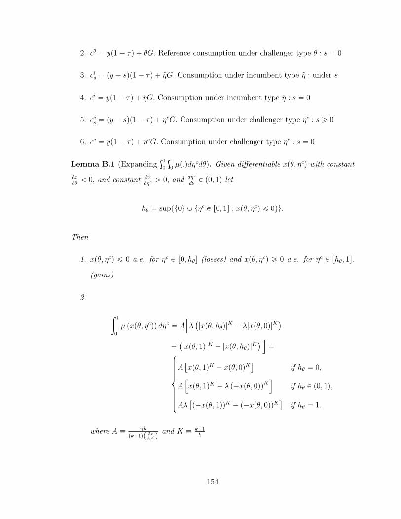
2. cθ “ yp1´ τq ` θG. Reference consumption under challenger type θ : s “ 0

3. cis “ py ´ sqp1´ τq ` ηG. Consumption under incumbent type η : under s

4. ci “ yp1´ τq ` ηG. Consumption under incumbent type η : s “ 0

5. ccs “ py ´ sqp1´ τq ` ηcG. Consumption under challenger type ηc : s ě 0

6. cc “ yp1´ τq ` ηcG. Consumption under challenger type ηc : s “ 0

Lemma B.1 (Expandingş1

0

ş1

0µp.qdηcdθ). Given differentiable xpθ, ηcq with constant

BxBθă 0, and constant Bx

Bηcą 0, and dηc

dθP p0, 1q let

hθ “ suptt0u Y tηc P r0, 1s : xpθ, ηcq ď 0uu.

Then

1. xpθ, ηcq ď 0 a.e. for ηc P r0, hθs (losses) and xpθ, ηcq ě 0 a.e. for ηc P rhθ, 1s.

(gains)

2.

ż 1

0

µ pxpθ, ηcqq dηc “ A”

λ`

|xpθ, hθq|K´ λ|xpθ, 0q|K

˘

``

|xpθ, 1q|K ´ |xpθ, hθq|K˘

ı

“$

’

’

’

’

’

’

&

’

’

’

’

’

’

%

A“

xpθ, 1qK ´ xpθ, 0qK‰

if hθ “ 0,

A”

xpθ, 1qK ´ λ p´xpθ, 0qqKı

if hθ P p0, 1q,

Aλ“

p´xpθ, 1qqK ´ p´xpθ, 0qqK‰

if hθ “ 1.

where A ” γk

pk`1qp BxBηc qand K ” k`1

k

154

3. Let

Θ “ suptt0u Y tθ P r0, 1s : hθ “ 0uu

Θ “ inftt1u Y tθ P r0, 1s : hθ “ 1uu.

Then hθ “ 0 a.e. for θ P r0,Θs, hθ P p0, 1q a.e. for θ P rΘ,Θs and hθ “ 1 a.e.

for θ P rΘ, 1s.

4.

1

B

ż 1

0

ż 1

0

µ pxpθ, ηcqq dηcdθ “$

’

’

’

’

’

’

’

’

’

’

’

’

’

’

’

’

’

’

’

’

’

’

&

’

’

’

’

’

’

’

’

’

’

’

’

’

’

’

’

’

’

’

’

’

’

%

xp1, 0qL ´ xp0, 0qL ´ xp1, 1qL ` xp0, 1qL if Θ “ Θ “ 1,

´λp´xp1, 0qqL ´ xp0, 0qL ´ xp1, 1qL ` xp0, 1qL if Θ P r0, 1q,Θ “ 1,

´λp´xp1, 0qqL ` λ p´xp0, 0qqL ´ xp1, 1qL ` xp0, 1qL if Θ “ 0,Θ “ 1,

´λp´xp1, 0qqL ` λ p´xp0, 0qqL ` λ p´xp1, 1qqL `xp0, 1qL

if Θ “ 0,Θ P p0, 1s,

´λp´xp1, 0qqL ` λ p´xp0, 0qqL ` λ p´xp1, 1qqL ´λ`

´xpΘ, 1q˘L

if Θ “ Θ “ 0.

Where B ” γk2

pk`1qpk`2qp´ BxBθBxBηc q

, L ” 2k`1k

.

Proof. 1. If xpθ, 0q ě 0, then xpθ, ηcq ą 0 for all ηc P p0, 1s because BxBηc

ą 0. Thus,

hθ “ 0 by construction and xpθ, ηcq ě 0 for all ηc P rhθ, 1s “ r0, 1s. Since r0, hθs “ r0, 0s

is measure 0, xpθ, ηcq ď 0 a.e. on r0, hθs.

If xpθ, 1q ď 0, then xpθ, ηcq ă 0 for all ηc P r0, 1q because BxBηcą 0. Thus, hθ “ 1

by construction and xpθ, ηcq ď 0 for all ηc P r0, hθs “ r0, 1s. Since rhθ, 1s “ r1, 1s is

measure 0, xpθ, ηcq ě 0 a.e. on rhθ, 1s.

155

Otherwise, xpθ, 0q ă 0 and xpθ, 1q ą 0. Since xpθ, .q is continuous (it’s differ-

entiable), then by IVT 0 ă hθ ă 1 satisfies xpθ, hθq “ 0. Since BxBηc

ą 0, we get

xpθ, ηcq ą 0 for all ηc P phθ, 1s and xpθ, ηcq ă 0 for all ηc P r0, hθq.

2. Using the above results, we can evaluate the inner gain-loss integral of µpxq on

ηc P r0, 1s :

ż 1

0

µ pxpθ, ηcqq dηc “ γ

ˆż 1

hθ

|x|1{kdηc ´ λ

ż hθ

0

|x|1{kdηc˙

“

$

’

’

’

’

’

’

&

’

’

’

’

’

’

%

´γλş1

0p´xq1{kdηc if hθ “ 1,

γş1

hθx1{kdηc ´ γλ

şhθ0p´xq1{kdηc if hθ P p0, 1q,

γş1

0x1{kdηc if hθ “ 0.

Because BxBηc

is a constant, we can sum the gains for cases when hθ P r0, 1q:

ż 1

hθ

x1{k

˜

BxBηc

BxBηc

¸

dηc “1BxBηc

ż 1

hθ

x1{k Bx

Bηcdηc “

k

pk ` 1q BxBηc

“

xpθ, 1qp1`kq{k ´ xpθ, hθqp1`kq{k

‰

Similarly, sum the losses for cases when hθ P p0, 1s:

ż hθ

0

p´xq1{k

˜

´ BxBηc

´ BxBηc

¸

dηc “k

pk ` 1q´

´ BxBηc

¯

”

p´xpθ, hθqqp1`kq{k

´ p´xpθ, 0qqp1`kq{kı

“k

pk ` 1q BxBηc

”

p´xpθ, 0qqp1`kq{k ´ p´xpθ, hθqqp1`kq{k

ı

Combining, this evaluates the integral as stated.

3. Observe that hθ is weakly increasing in θ because BxBθă 0. It is strictly increasing

along xpθ, hθq “ 0 with slope dηc

dθP p0, 1q by assumption.

156

Case I: h1 “ h0 “ 0 ùñ hθ “ 0 for all θ P r0, 1s, and Θ “ Θ “ 1. Then hθ “ 0 on

r0,Θs “ r0, 1s, while rΘ,Θs “ r1, 1s and rΘ, 1s “ r1, 1s are measure 0.

Case II: h1 P p0, 1q, while h0 “ 0. Then 0 ď Θ ă 1 and Θ “ 1. This means hθ “ 0

on r0,Θs, while hθ P p0, 1q on pΘ,Θs “ pΘ, 1s and rΘ, 1s “ r1, 1s is measure 0.

Case III: h1 P p0, 1q, while h0 P p0, 1q ùñ hθ P p0, 1q for all θ P r0, 1s. Then

Θ “ 0 and Θ “ 1. This means hθ P p0, 1q on rΘ,Θs “ r0, 1s, while r0,Θs “ r0, 0s and

rΘ, 1s “ r1, 1s are measure 0.

Case IV: h1 “ 1, while h0 P p0, 1q. Then Θ “ 0 and 0 ă Θ ď 1. This means

hθ P p0, 1q on rΘ,Θq “ r0,Θq, while hθ “ 1 on rΘ, 1s and r0,Θs “ r0, 0s is measure 0.

Case V: h1 “ h0 “ 1 ùñ hθ “ 1 for all θ P r0, 1s, and Θ “ Θ “ 0. Then hθ “ 1 on

rΘ, 1s “ r0, 1s, while r0,Θs “ r0, 0s and rΘ,Θs “ r0, 0s are measure 0.

4. Using the values of the inner integral from part (2), Ipθ, hθq, can evaluate the

outer integral as follows:

I “

ż 1

0

Ipθ, hθqdθ “

ż Θ

0

Ipθ, hθqdθ `

ż Θ

Θ

Ipθ, hθqdθ `

ż 1

Θ

Ipθ, hθqdθ (B.1.1)

hθ “ 0 a.e. for all θ P r0,Θs:

ż Θ

0

Ipθ, hθqdθ “

ż Θ

0

A“

xpθ, 1qK ´ xpθ, 0qK‰

dθ

“Ak

pk ` 2q`

´BxBθ

˘

`“

xpΘ, 0qL ´ xp0, 0qL‰

´“

xpΘ, 1qL ´ xp0, 1qL‰˘

(B.1.2)

“Ak

pk ` 2q`

´BxBθ

˘

`“

|xpΘ, 0q|L ´ |xp0, 0q|L‰

´“

|xpΘ, 1q|L ´ |xp0, 1q|L‰˘

(B.1.3)

because BxBθ

was assumed to be constant and L ” 2k`1k. Observe that Eq. (B.1.2)

expression is valid for Θ ą 0 and equal to 0 for Θ “ 0. In the later case, x under the

fractional power may be negative, so to keep the same expression valid for both cases

(for all Θ), we can impose absolute values under the power.

157

Similarly, hθ P p0, 1q a.e. for all θ P rΘ,Θs:

ż Θ

Θ

Ipθ, hθqdθ “

ż Θ

Θ

A”

xpθ, 1qK ´ λ p´xpθ, 0qqKı

dθ

“Ak

pk ` 2q`

´BxBθ

˘

´

λ”

p| ´ xpΘ, 0q|qL ´`

| ´ xpΘ, 0q|˘Lı

´“

|xpΘ, 1q|L ´ |xpΘ, 1q|L‰

¯

(B.1.4)

Similarly, hθ “ 1 a.e. for all θ P rΘ, 1s:

ż 1

Θ

Ipθ, hθqdθ “

ż 1

Θ

Aλ“

p| ´ xpθ, 1q|qK ´ p| ´ xpθ, 0q|qK‰

dθ

“Akλ

pk ` 2q`

´BxBθ

˘

´

p| ´ xp1, 1q|qL ´`

| ´ xpΘ, 1q|˘L´ p| ´ xp1, 0q|qL ` p| ´ xpΘ, 0q|qL

¯

(B.1.5)

Let B ” Akk`2

“γk2

pk`1qpk`2qp´ BxBθBxBηc q

. I in Eq. (B.1.1) by adding equations (B.1.2)-

(B.1.5) and simplifying 4 extra terms.

1

B

ż 1

0

ż 1

0

µ pxpθ, ηcqq dηcdθ “ |xpΘ, 0q|L ´ |xp0, 0q|L ` |xp0, 1q|L ` λ p| ´ xpΘ, 0q|qL

´|xpΘ, 1q|L ` λ p| ´ xp1, 1q|qL ´ λ`

| ´ xpΘ, 1q|˘L´ λp| ´ xp1, 0q|qL

(B.1.6)

Eq. (B.1.6) is valid for all Θ P r0, 1s and for all Θ P r0, 1s. The sum of 8 terms

always reduces to the values of the function x at the four corners of the unit square

when Θ,Θ are known. The following two facts are used: corner solutions (such

as Θ “ 0) are substituted directly and interior solutions (such Θ P p0, 1s) satisfy

xp¨, ¨q “ 0. The five cases from part (3) are:

158

1

B

ż 1

0

ż 1

0

µ pxpθ, ηcqq dηcdθ “$

’

’

’

’

’

’

’

’

’

’

’

’

’

’

’

’

’

’

&

’

’

’

’

’

’

’

’

’

’

’

’

’

’

’

’

’

’

%

xp1, 0qL ´ xp0, 0qL ´ xp1, 1qL ` xp0, 1qL if Θ “ Θ “ 1,

´λp´xp1, 0qqL ´ xp0, 0qL ´ xp1, 1qL ` xp0, 1qL if Θ P r0, 1q,Θ “ 1,

´λp´xp1, 0qqL ` λ p´xp0, 0qqL ´ xp1, 1qL ` xp0, 1qL if Θ “ 0,Θ “ 1,

´λp´xp1, 0qqL ` λ p´xp0, 0qqL ` λ p´xp1, 1qqL ` xp0, 1qL if Θ “ 0,Θ P p0, 1s,

´λp´xp1, 0qqL ` λ p´xp0, 0qqL ` λ p´xp1, 1qqL ´ λ`

´xpΘ, 1q˘L

if Θ “ Θ “ 0.

In the first case, x is positive at four corners of the unit square. In the second case,

xp1, 0q ă 0 is the only negative corner. In the third case, xp0, 0q ă 0 and xp1, 0q ă 0

(the slope 0 ă dηc

dθă 1 along x “ 0 by assumption, and thus xp1, 0q ą 0 here). In

the fourth case, xp1, 1q ă 0 also. In the fifth case, all corners are negative. The

corresponding element is scaled by ´λ for each transition.

The next corollary highlights the importance of the assumptions that dxdθ‰ 0 and

dxdηc‰ 0.

Corollary B.2. 1. Given differentiable xpθq with constant dxdθ“ dx

dηc“ 0,

ż 1

0

ż 1

0

µ pxpθ, ηcqq dηcdθ “ µ pxq “

$

’

’

&

’

’

%

γx1k if x ą 0,

´γλp´xq1k if x ď 0.

159

2. Constant dxdθ“ 0 and constant dx

dηcą 0.

ż 1

0

ż 1

0

µ pxpθ, ηcqq dηcdθ “

$

’

’

’

’

’

’

&

’

’

’

’

’

’

%

A“

xp1qK ´ xp0qK‰

if h “ 0,

A”

xp1qK ´ λ p´xp0qqKı

if h P p0, 1q,

Aλ“

p´xp1qqK ´ p´xp0qqK‰

if h “ 1.

where A ” γk

pk`1qp BxBηc q

First, consider the no-shock state. Let xcppθ, ηc; s, ηq “ cc´cp be the gain-loss input

of the µ. The challenge is to consider the set of points where the argument switches

signs because of the λ kink in µ. Observe that cc is independent of s, while cp depends

on s. This means as s goes up, reference point looks worse and worse relative to the

actual consumption and so the gains grow at any point in the parameter space.

Here we verify thatBxcpBθ

satisfies B.1 condition (constant and negative).

BxcpBθ

“ 0´BcpBθ

“ ´pQsBcθsBθ´ p1´ pqq

dcθ

dθ“ ´G ppQs ` p1´ pqqq ă 0 (B.1.7)

Similarly, verify thatBxcpBηc

satisfies B.1 condition (constant and positive).

BxcpBηc

“ G ą 0 (B.1.8)

Thus,´BxcpBθ

BxcpBηc

“ pQs`p1´ pqq P p0, 1q also holds as long as both q,Qs are not equal

to 0 or both equal to 1. That is, both the challenger and the incumbent have an

interior probability of being chosen in each state.

160

Furthermore, we calculateBxcpBη

:

BxcpBη

“ 0´BcpBη

“ G r´pp1´Qsq ´ p1´ pqp1´ qqs ă 0 (B.1.9)

If q and Qs are not both identically 0, then reference point is not identical to

picking incumbent for sure:BxcpBθă 0. If q,Qs are not both equal to 1, then

BxcpBηą 0

Otherwise, when q “ Qs “ 0, we haveBxcpBθ“ 0 and when q “ Qs “ 1, then

BxcpBη“ 0

(the reference point doesn’t depend on incumbent when challenger is always picked).

Likewise, we calculateBxcpBs

for p ą 0 :

BxcpBs

“ 0´BcpBs

“ ´pQsBcθsBs´ pp1´Qsq

BcisBs“ pp1´ τq ą 0 (B.1.10)

Let

hcθps, ηq “ suptt0u Y tηc P r0, 1s : xcppθ, ηc; s, ηq ď 0uu (B.1.11)

Given ps, ηq, hcθ describes the largest ηc until xcp hits gains or it’s equal to 0 if gains

happen for all ηc.

Since

xcpp0, 1; s, 1q ą xcpp1, 1; s, 1q “

“ yp1´ τq `G´ pppy ´ sqp1´ τq `Gq ´ p1´ pqpyp1´ τq `Gq

“ psp1´ τq ą 0, (B.1.12)

then @η P r0, 1s, xcpp1, 1; s, ηq ą 0 and xcpp1, 1; s, ηq ą 0 becauseBxcpBηą 0.

In words, we know that given a reference draw of the best challenger mixed with

the best incumbent and picking the best (actual) challenger, there will be maximal

G of public goods in both reference point and in the actual draw. The challenger is

better because no shock has happened but the shock has p ą 0 weight in the reference

161

point. This means any incumbent’s ability less than 1 will lead to even larger gains.

If the reference challenger was worse, θ “ 0, the gains grow. By continuity of payoffs

in ηc and strict inequality (for p ą 0, s ą 0), we can choose ηc ă 1 so that loss is still

strictly positive.

This shows:

@θ P r0, 1s, @s ą 0, @η P r0, 1s, hcθps, ηq ă 1. (B.1.13)

The cutoff boundary between gains and losses is strictly to below the top of the unit

square where ηc “ 1. As s goes up´

BxcpBsą 0

¯

, hcθ moves further down.

As in part (3) of Lemma B.1, the following cutoffs describe either the location of

the interior kink in hcθ or its corners:

Θcps, ηq “ suptt0u Y tθ P r0, 1s : hcθps, ηq “ 0uu (B.1.14)

Θcps, ηq “ inftt1u Y tθ P r0, 1s : hcθps, ηq “ 1uu. (B.1.15)

The restriction that xc imposes on hcθ P r0, 1q corresponds to cases I-III of Lemma

B.1. In particular,

Θcps, ηq “ 1. (B.1.16)

Meanwhile, there is no restriction on Θcps, ηq P r0, 1s. This reduces to a one-

dimensional problem similar to the incumbent’s case without shock, except in that

case Θi is restricted to away from a corner, so the single remaining corner gave a single

condition H ipsq on η when that corner was attained. In contrast, the challenger’s

problem allows for both Θcps, ηq “ 0 and Θc

ps, ηq “ 1, which defines two separate

boundary cutoffs for η as follows:

162

Hcpsq “ suptt0u Y tη P r0, 1s : Θc

ps, ηq “ 1uu (B.1.17)

Hcpsq “ inftt1u Y tη P r0, 1s : Θc

ps, ηq “ 0uu (B.1.18)

As η grows, xcp decreases becauseBxcpBηă 0. Then Hc

psq is the cutoff for η, be-

low which for all η P r0, Hcpsqq, get Θc

ps, ηq “ 1, which says that xcp “ 0 bound-

ary intersects the right edge of the unit square and through its bottom-left cor-

ner for η “ Hcpsq. Moreover, hcθps, ηq “ 0 for all θ P r0, 1s. Hence, for all ηc P

r0, 1s, xcppθ, ηc; s, ηq ě 0. In other words, there are gains for all ηc, for all θ (every-

where on the unit square), whenever η is below the Hcpsq cutoff. This corresponds

to case I boundary from part (3) of Lemma B.1.

Similarly, Hcpsq is the cutoff for η, above which for all η P pH

cpsq, 1s,Θc

ps, ηq “ 0,

which says that xcp “ 0 boundary intersects the left edge of the unit square and

through its bottom-left corner for η “ Hcpsq. Moreover, hcθps, ηq ą 0 for all θ P r0, 1s.1

Hence, for all ηc P rhcθps, ηq, 1s, there are gains xcp pθ, ηc; s, ηq ě 0. In contrast, for all

ηc P r0, hcθps, ηqs, there are losses xcp pθ, ηc; s, ηq ď 0, whenever η is above the H

cpsq

cutoff. Thus, the top two corners of the unit square involve gains and the bottom

two corners involve losses. This corresponds to case III boundary from part (3) of

Lemma B.1.

Otherwise, η P rHcpsq, H

cpsqs. This corresponds to a loss at bottom-right corner

xpcp1, 0; s, ηq ă 0, and a gain for the other three corners. This is case II boundary

from part (3) of Lemma B.1.

1When θ P p0, 1s, hcθps, ηq ą 0 because Θcps, ηq “ 0 directly. It’s also true for θ “ 0 by continuity

of xcp “ 0 boundary in η (xcp is decreasing) and in ηc (xcp is increasing). Note that hc0ps,Hcpsqq “ 0

means xcpp0, hc0ps,H

cpsqq; s,H

cpsqq “ 0 implies hc0ps, ηq ą 0 for all η ą H

cpsq.

163

Let

Sc “ supts : Hcpsq ă 1u (B.1.19)

Sc“ supts : H

cpsq ă 1u (B.1.20)

which are positive because Hcp0q “ H

cp0q “ 0. Note that Hc

psq ď overlineHcpsq for

all s, so it’s enough to show that Sc is finite as that implies 1 “ HcpScq ď H

cpScq ď 1,

and Sc is an upper bound for Sc. Sc is finite because

BxcpBs“ pp1 ´ τq ą 0. Thus, we

get an upper bound2 for Sc ď S: for S large enough, xcpp1, 0; S, 1q ě 0. Then

hc1pS, 1q “ 0 ùñ ΘpS, 1q “ 1 ùñ HcpSq “ 1.

This Sc is the cutoff when Hcpsq “ 1 for all s ą Sc. Similarly, S

cis the cutoff when

Hcpsq “ 1 for all s ą S

c.

Figure B.1 shows the Hcpsq and H

cpsq boundaries in the s ˆ η region of the

parameter space for a low probability of shock with p “ 1100

. The illustrated boundary

is similar to the “surprise” shock special case. In general, for fixed p, Hcpsq and H

cpsq

split the sˆ η space into three sections.

The upper-left section, satisfying s ă Sc

with Hcpsq ą 0, is a set of points ps, ηq

that satisfy Hcpsq ă η ď 1. For these points, xcpp¨, ¨; s, ηq “ 0 forms a case III boundary

in the θˆ ηc space from part (3) of Lemma B.1 with losses at the bottom two corners

of the unit square and gains at the top two. Since Θcps, ηq “ 0 and for all θ P r0, 1s,

we have hcθps, ηq P p0, 1q meaning there are strict gains on phcθps, ηq, 1s and strict losses

on r0, hcθps, ηqq.

The middle section, is a set of points ps, ηq that satisfy Hcpsq ă η ă H

cpsq. For

these points, xcpp¨, ¨; s, ηq “ 0 forms a case II boundary in the θ ˆ ηc space from part

2This upper bound S requires that for s ą S, there are gains everywhere on the unit square, inparticular at the bottom right corner for the worst challenger against the best incumbent.

164

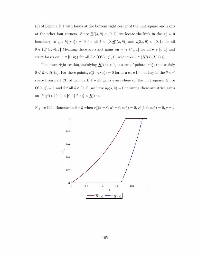
(3) of Lemma B.1 with losses at the bottom right corner of the unit square and gains

at the other four corners. Since Θcps, ηq P p0, 1q, we locate the kink in the xcp “ 0

boundary to get hcθps, ηq “ 0 for all θ P r0,Θcps, ηqs and hcθps, ηq P p0, 1q for all

θ P pΘcps, ηq, 1s Meaning there are strict gains on ηc P phcθ, 1s for all θ P r0, 1s and

strict losses on ηc P r0, hcθq for all θ P pΘcps, ηq, 1s, whenever η P pHc

psq, Hcpsqq.

The lower-right section, satisfying Hcpsq ă 1, is a set of points ps, ηq that satisfy

0 ď η ă Hcpsq. For these points, xcpp¨, ¨; s, ηq “ 0 forms a case I boundary in the θˆηc

space from part (3) of Lemma B.1 with gains everywhere on the unit square. Since

Θcps, ηq “ 1 and for all θ P r0, 1s, we have hθps, ηq “ 0 meaning there are strict gains

on pθ, ηcq P r0, 1s ˆ r0, 1s for η ă Hcpsq.

Figure B.1: Boundaries for η when xcppθ “ 0, ηc “ 0; s, ηq “ 0, xcpp1, 0; s, ηq “ 0, p “ 12

165

Picking challenger’s lottery subject to reference compound lottery cp and shock

s ě 0.

Upcc|cp; s, ηq “´

p1´ τqpy ´ sq `1

2G¯

`γk2

pk ` 1qp2k ` 1q´

´Bxcppθ,η

cq

Bθ

¯´

Bxcppθ,ηcq

Bηc

¯Icppsq (B.1.21)

where the integral Icppsq on the right-hand side depends on the four values of the xcpp¨, ¨q

at corners of the pθ, ηcq P t0, 1u ˆ t0, 1us and the functional form switches between

gains and losses at the two boundaries of the parameters: Hcpsq, Hc

psq where µpxcpq

vanishes. Combining the boundary analysis in the Figure B.1 with B.1 get:

Icpps, ηq “

$

’

’

’

’

’

’

’

’

’

’

’

’

’

’

’

’

’

’

&

’

’

’

’

’

’

’

’

’

’

’

’

’

’

’

’

’

’

%

´λp´xcpp1, 0qqL ` λp´xcpp0, 0qq

L ´ xcpp1, 1qL `xcpp0, 1q

L

if Hcpsq ď η ď 1

´λp´xcpp1, 0qqL ´ xcpp0, 0q

L ´ xcpp1, 1qL `xcpp0, 1q

L

if Hcpsq ď η ď H

cpsq

xcpp1, 0qL ´ xcpp0, 0q

L ´ xcpp1, 1qL `xcpp0, 1q

L

if 0 ď η ď Hcpsq

where L ” 2k`1k.

Characterising Challenger’s Utility, given shock

Second, consider the shock state.

Let xcsp pθ; s, ηq “ ccs´ cp. Here we verify thatBxcspBθ

satisfies B.1 condition (constant

and negative).

166

BxcspBθ

“ 0´BcpBθ

“ ´pQsBcθsBθ´ p1´ pqq

dcθ

dθ“ ´G ppQs ` p1´ pqqq ă 0 (B.1.22)

Similarly, verify thatBxcspBηc

satisfies B.1 condition (constant and positive).

BxcspBηc

“ G ą 0 (B.1.23)

Thus,´BxcspBθ

BxcspBηc

“ pQs ` p1 ´ pqq P p0, 1q also holds as long as both q,Qs are not

equal to 0 or both equal to 1. That is, both the challenger and the incumbent have

an interior probability of being chosen in each state.

Furthermore, we calculateBxcspBη

:

BxcspBη

“ 0´BcpBη

“ G r´pp1´Qsq ´ p1´ pqp1´ qqs ă 0 (B.1.24)

If q and Qs are not both identically 0, then reference point is not identical to

picking incumbent for sure:BxcspBθă 0. If q,Qs are not both equal to 1, then

BxcspBηą 0

Otherwise, when q “ Qs “ 0, we haveBxcspBθ“ 0 and when q “ Qs “ 1, then

BxcspBη“ 0

(the reference point doesn’t depend on incumbent when challenger is always picked).

Likewise, we calculateBxcspBs

for p ą 0 :

BxcspBs

“ ´p1´ τq ´BcpBs

“ ´pQsBcθsBs´ pp1´Qsq

BcisBs“ ´p1´ pqp1´ τq ă 0 (B.1.25)

Let

hcsθ ps, ηq “ inftt1u Y tηc P r0, 1s : xcsp pθ, ηc; s, ηq ě 0uu (B.1.26)

Given ps, ηq, hcsθ describes the smallest ηc until xcsp hits losses or it’s equal to 1 if

losses happen for all ηc.

167

Since

xcsp p1, 0; s, 0q ă xcsp p0, 0; s, 0q “

“ py ´ sqp1´ τq ´ pppy ´ sqp1´ τqq ´ p1´ pqpyp1´ τqq

“ ´sp1´ τq ` psp1´ τq “ ´p1´ pqp1´ τq ă 0, (B.1.27)

then @η P r0, 1s, xcsp p1, 0; s, ηq ă 0 and xcsp p0, 0; s, ηq ă 0 becauseBxcspBηă 0.

In words, we know that given a reference draw of the worst challenger mixed

with the the worst incumbent and picking the worst (actual) challenger, there will

be no public goods in both reference point and in the actual draw. The challenger

is a loss because the shock has happened but this shock has a smaller weight p ă 1

in the reference point and the after-tax income is higher. This means any positive

incumbent’s ability will lead to even larger losses. If the reference challenger was

better, θ “ 1, the losses grow. By continuity of payoffs in ηc and strict inequality (for

p ą 0, s ą 0), we can choose a slightly better challenger with ηc ą 0 so that there is

still a strict loss.

This shows:

@θ P r0, 1s, @s ą 0, @η P r0, 1s, hcsθ ps, ηq ą 0. (B.1.28)

The cutoff boundary between gains and losses is strictly to above the bottom of the

unit square where ηc “ 0. As s goes up´

BxcspBsă 0

¯

, hcsθ moves further up.

As in part (3) of Lemma B.1, the following cutoffs describe either the location of

the interior kink in hcsθ or its corners:

168

Θcsps, ηq “ suptt0u Y tθ P r0, 1s : hcsθ ps, ηq “ 0uu (B.1.29)

Θcsps, ηq “ inftt1u Y tθ P r0, 1s : hcθps, ηq “ 1uu. (B.1.30)

The restriction that xcs imposes on hcsθ P p0, 1s corresponds to cases III-V of

Lemma B.1. In particular,

Θcsps, ηq “ 0. (B.1.31)

Meanwhile, there is no restriction on Θcsps, ηq P r0, 1s. This reduces to a one-

dimensional problem similar to the incumbent’s case with shock, except in that case

Θis is restricted to away from a corner, so the single remaining corner gave a single

condition H ispsq on η when that corner was attained. In contrast, the challenger’s

problem allows for both Θcsps, ηq “ 0 and Θ

csps, ηq “ 1, as well as intermediate values.

The challenger’s problem with shock is a mirror of the challenger’s problem without

the shock in the sense that it covers boundary cases III-V, rather than I-III. With

shock, the xcsp “ 0 boundary is uniformly bounded away from ηc “ 0, the bottom of

the unit square, while without the shock this boundary xcp “ 0 is uniformly bounded

away from ηc “ 1, the top of the unit square. We define these two separate boundary

cutoffs for η as follows:

Hcspsq “ suptt0u Y tη P r0, 1s : Θ

csps, ηq “ 1uu (B.1.32)

Hcspsq “ inftt1u Y tη P r0, 1s : Θ

csps, ηq “ 0uu (B.1.33)

As η grows, xcsp decreases (losses grow) becauseBxcspBη

ă 0. Then, Hcspsq is the

cutoff for η, below which for all η P r0, Hcspsqq, get Θ

csps, ηq “ 1, which says that

xcsp “ 0 boundary intersects the right edge of the unit square and through its top-right

169

corner for η “ Hcspsq. Moreover, hcsθ ps, ηq ă 1 for all θ P r0, 1s.3 Hence, for all ηc P

rhcsθ ps, ηq, 1s, there are gains xcsp pθ, ηc; s, ηq ě 0. In contrast, for all ηc P r0, hcsθ ps, ηqs,

there are losses xcsp pθ, ηc; s, ηq ď 0, whenever η is below the Hcs

psq cutoff. Thus, the

top two corners of the unit square involve gains and the bottom two corners involve

losses. This corresponds to case III boundary from part (3) of Lemma B.1.

Similarly, Hcspsq is the cutoff for η, above which for all η P r0, Hcs

psqq, get

Θcsps, ηq “ 0 which says that xcsp “ 0 boundary intersects the left edge of the unit

square and through its top-left corner for η “ Hcspsq. Moreover, hcsθ ps, ηq “ 1 for all

θ P r0, 1s. Hence, for all ηc P r0, 1s, xcsp pθ, ηc; s, ηq ď 0. In other words, there are losses

for all ηc, for all θ (everywhere on the unit square), whenever η is above the Hcspsq

cutoff. This corresponds to case V boundary from part (3) of Lemma B.1.

Otherwise, η P rHcspsq, H

cspsqs. This corresponds to a gain at top-left corner

xpcp0, 1; s, ηq ą 0, and a loss for the other three corners. This is case IV boundary

from part (3) of Lemma B.1.

Let

Scs “ supts : Hcspsq ą 0u (B.1.34)

Scs“ supts : H

cspsq ą 0u (B.1.35)

which are positive because Hcsp0q “ H

csp0q “ 1. Note that Hcs

psq ď overlineHcspsq

for all s, so it’s enough to show that Scs

is finite as that implies 0 ď HcspScsq ď

Hcs `

Scs˘“ 0, and S

csis an upper bound for Scs. S

csis finite because

BxcspBs“ ´p1 ´

pqp1 ´ τq ă 0. Thus, we get an upper bound4 for Scsď S as follows: for S large

3When θ P r0, 1q, hcsθ ps, ηq ă 1 because Θcsps, ηq “ 1 directly. It’s also true for θ “ 1 by

continuity of xcsp “ 0 boundary in η (xcsp is decreasing) and in ηc (xcsp is increasing). Note thathcs0 ps,H

cspsqq “ 1 means xcsp p0, h

cs0 ps,H

cspsqq; s,Hcs

psqq “ 0 implies hcs1 ps, ηq ă 1 for all η ă Hcspsq.

4This upper bound S requires that for s ą S, there are losses everywhere on the unit square, inparticular at the top-left corner for the best (actual) challenger against the worst incumbent mixedwith the worst reference challenger.

170

enough, xcsp p0, 1; S, 0q ď 0. Then

hcs0 pS, 0q “ 1 ùñ ΘpS, 0q “ 0 ùñ HcspSq “ 0.

This Scs

is the cutoff when Hcspsq “ 1 for all s ą Scs. Similarly, Scs is the cutoff

when Hcspsq “ 1 for all s ą Scs.

Figure B.2 shows the Hcspsq and H

cspsq boundaries in the s ˆ η region of the

parameter space for a low probability of shock with p “ 1100

. The illustrated boundary

is similar to the “surprise” shock special case. In general, for fixed p, Hcspsq and

Hcspsq split the sˆ η space into three sections.

The lower-left section, satisfying s ă Scs

with Hcspsq ą 0, is a set of points ps, ηq

that satisfy 0 ď η ă Hcspsq. For these points, xcsp p¨, ¨; s, ηq “ 0 forms a case III

boundary in the θ ˆ ηc space from part (3) of Lemma B.1 with losses at the bottom

two corners of the unit square and gains at the top two. Since Θcsps, ηq “ 1 and for

all θ P r0, 1s, we have hcsθ ps, ηq P p0, 1q meaning there are strict gains on phcsθ ps, ηq, 1s

and strict losses on r0, hcsθ ps, ηqq.

The middle section, is a set of points ps, ηq that satisfy Hcspsq ă η ă H

cspsq. For

these points, xcsp p¨, ¨; s, ηq “ 0 forms a case IV boundary in the θˆ ηc space from part

(3) of Lemma B.1 with gains at the top-left corner of the unit square and losses at

the other four corners. Since Θcsps, ηq P p0, 1q, we locate the kink in the xcsp “ 0

boundary to get hcsθ ps, ηq “ 1 for all θ P rΘcsps, ηq, 1s and hcsθ ps, ηq P p0, 1q for all

θ P r0,Θcsps, ηqq. This means there are strict losses on ηc P r0, hcsθ q for all θ P r0, 1s

and strict gains on ηc P phcsθ , 1s for all θ P r0,Θcsps, ηqq, whenever η P pHcs

psq, Hcspsqq.

The upper-right section, is a set of points ps, ηq that satisfy Hcspsq ă η ď 1. For these

points, xcsp p¨, ¨; s, ηq “ 0 forms a case V boundary in the θˆ ηc space from part (3) of

Lemma B.1 with losses everywhere on the unit square. Since Θcsps, ηq “ 0 and for all

171

θ P r0, 1s, we have hθps, ηq “ 1 meaning there are strict losses on pθ, ηcq P r0, 1sˆr0, 1s

for η ą Hcspsq.

Figure B.2: Boundaries for η when xcsp pθ “ 0, ηc “ 1; s, ηq “ 0, xcsp p1, 1; s, ηq “ 0, p “1

100

By Lemma B.1 and Figure B.2, we can evaluate the utility function that cor-

responds to picking the challenger when the shock happens, subject to reference

compound lottery cp and shock s ě 0. Recall that xisp pθ; s, ηq “ cis ´ cp.

Upccs|cp; sq “ p1´ τqy `1

2G

`γk2

pk ` 1qp2k ` 1q´

´Bxcsp pθ,η

cq

Bθ

¯´

Bxcsp pθ,ηcq

Bηc

¯Icsp psq (B.1.36)

where the integral Icsp psq on the right-hand side depends on the four values of the

xcsp p¨, ¨q at corners of the pθ, ηcq P t0, 1u ˆ t0, 1us and the functional form switches

between gains and losses at the two boundaries of the parameters: Hcspsq, Hcs

psq

where µpxcsp q vanishes.

172

Icsp ps, ηq “

$

’

’

’

’

’

’

’

’

’

’

’

’

’

’

’

’

’

’

&

’

’

’

’

’

’

’

’

’

’

’

’

’

’

’

’

’

’

%

xcsp0, 1qL ´ xcsp1, 1qL ` λp´xcsp0, 0qqL ´ λp´xcsp1, 0qqL

if 0 ď η ď Hcspsq.

xcsp0, 1qL ` λp´xcsp1, 1qqL ` λp´xcsp0, 0qqL ´ λp´xcsp1, 0qqL

if Hcspsq ď η ď H

cspsq

´λp´xcsp0, 1qqL ` λp´xcsp1, 1qqL ` λp´xcsp0, 0qqL ´ λp´xcsp1, 0qqL

if Hcspsq ď η ď 1

where L ” 2k`1k.

Characterising Incumbent’s Utility, given no shock

Let reference point be

cp “ ppQscθs ` p1´Qsqc

isq ` p1´ pqpqc

θ` p1´ qqciq

where with probability p the voter will learn there is s shock next period before voting

and with probability 1 ´ p he learns there will be no shock next period. Qs is the

cutoff for incumbent, when shock happens and q the cutoff when no shock happens.

Here θ ability emphasizes a hypothetical draw of the challenger in the reference point,

distinct from ccs which would be an actual draw (different and independent of θ).

For brevity of notation define, G “ αpτy ´ rq is the coefficient of the ability in

making the public good.

The corresponding consumptions are:

1. cθs “ py´sqp1´ τq`θG. Reference consumption under challenger type θ : s ě 0

2. cθ “ yp1´ τq ` θG. Reference consumption under challenger type θ : s “ 0

173

3. cis “ py ´ sqp1´ τq ` ηG. Consumption under incumbent type η : s ě 0

4. ci “ yp1´ τq ` ηG. Consumption under incumbent type η : s “ 0

5. ccs “ py ´ sqp1´ τq ` ηcG. Consumption under challenger type ηc : s ě 0

6. cc “ yp1´ τq ` ηcG. Consumption under challenger type ηc : s “ 0

Recall that

µpxq “

$

’

’

&

’

’

%

γx1k if x ą 0,

´γλp´xq1k if x ď 0.

Lemma B.3 (Expandingş1

0µp.qdθ). Given differentiable xpθq with constant dx

dθă 0,

let

Θ “ suptt0u Y tθ P r0, 1s : xpθq ě 0uu.

Then

1. xpθq ě 0 a.e. for θ P r0,Θs (gains) and xpθq ď 0 a.e. for θ P rΘ, 1s. (losses) 2.

ż 1

0

µ pxpθqq dθ “ C“

´`

|xpΘq|K ´ |xp0q|K˘

´ λ`

|xp1q|K ´ |xpΘq|K˘‰

q “

$

’

’

’

’

’

’

&

’

’

’

’

’

’

%

Cλ”

p´xp0qqK ´ p´xp1qqKı

if Θ “ 0,

C”

xp0qK ´ λ p´xp1qqKı

if Θ P p0, 1q,

C“

xp0qK ´ xp1qK‰

if Θ “ 1.

where C ” γk

pk`1qp´ dxdθ q

and K ” k`1k

3. Let b “ |dxdθ|, then xpθq “ a´ bθ and Θ “

$

’

’

’

’

’

’

&

’

’

’

’

’

’

%

0 if a ď 0,

ab

if 0 ă a ă b,

1 if a ě b,

174

Proof. 1. If xp0q ď 0, then xpθq ă 0 for all θ P p0, 1s because dxdθă 0. Thus, Θ “ 0 by

construction and xpθq ď 0 for all θ P rΘ, 1s. Since r0,Θs “ r0, 0s is measure 0, xpθq ě 0

a.e. on r0,Θs.

If xp1q ě 0, then xpθq ą 0 for all θ P r0, 1q because dxdθă 0. Thus, Θ “ 1 by

construction and xpθq ě 0 for all θ P r0,Θs. Since rΘ, 1s “ r1, 1s is measure 0, xpθq ď 0

a.e. on rΘ, 1s.

Otherwise, xp0q ą 0 and xp1q ă 0. Since x is continuous (it’s differentiable), then

by IVT 0 ă Θ ă 1 satisfies xpΘq “ 0. Since dxdθă 0, we get xpθq ą 0 for all θ P r0,Θq

and xpθq ă 0 for all θ P pΘ, 1s.

2. Using the above results, we can evaluate the gain-loss integral of µpxq on

θ P r0, 1s :

ż 1

0

µ pxpθqq dθ “ γ

ˆż Θ

0

|x|1{kdθ ´ λ

ż 1

Θ

|x|1{kdθ

˙

“

$

’

’

’

’

’

’

&

’

’

’

’

’

’

%

´γλş1

0p´xq1{kdθ if Θ “ 0,

γşΘ

0x1{kdθ ´ γλ

ş1

Θp´xq1{kdθ if Θ P p0, 1q,

γş1

0x1{kdθ if Θ “ 1.

Because dxdθ

is a constant, we can sum the gains:

ż Θ

0

x1{kdxdθdxdθ

dθ “1dxdθ

ż Θ

0

x1{k dx

dθdθ “

´k

pk ` 1q`

´dxdθ

˘

“

xpΘqp1`kq{k ´ xp0qp1`kq{k‰

Similarly, sum the losses:

ż 1

Θ

p´xq1{k

˜

´dxdθ

´dxdθ

¸

dθ “k

pk ` 1q`

´dxdθ

˘

”

p´xp1qqp1`kq{k ´ p´xpΘqqp1`kq{kı

Combining, this evaluates the integral as stated.

175

3. Let a “ xp0q. Then

xpθq “

ż

dx

dθdθ “

dx

dθθ ` a

The Lemma B.3 shows that the value of the integral depends only on the value of

the function at the end-points, where the functional form changes based on whether Θ

(the split between the gains and losses) is at a corner Θ P t0, 1u or interior Θ P p0, 1q.

It does not depend on the specific value of Θ explicitly. However, because x was

assumed to be a linear function of θ, the situations when Θ is higher are precisely

when xp0q is higher.

The next corollary highlights the importance of the assumption that dxdθ‰ 0.

Corollary B.4. Given differentiable xpθq with constant dxdθ“ 0,

ż 1

0

µ pxpθqq dθ “ µ pxq “

$

’

’

&

’

’

%

γx1k if x ą 0,

´γλp´xq1k if x ď 0.

First, consider the no-shock state. Let xippθ; s, ηq “ ci ´ cp be the gain-loss input

of the µ. Here we calculateBxipBθ

:

BxipBθ

“ 0´BcpBθ

“ ´pQsBcθsBθ´ p1´ pqq

dcθ

dθ“ ´G ppQs ` p1´ pqqq ă 0 (B.1.37)

Furthermore, we calculateBxipBη

:

BxipBη

“Bci

Bη´BcpBη

“ G r1´ pp1´Qsq ´ p1´ pqp1´ qqs ą 0 (B.1.38)

176

If q and Qs are not both identically 0, then reference point is not identical to picking

incumbent for sure:BxipBθă 0 and

BxipBηą 0 Otherwise, when q “ Qs “ 0, we have

BxipBη“

BxipBθ“ 0.

Likewise, we calculateBxipBs

for p ą 0 :

BxipBs

“ 0´BcpBs

“ ´pQsBcθsBs´ pp1´Qsq

BcisBs“ pp1´ τq ą 0 (B.1.39)

The challenge is to consider the set of points where the argument switches signs

because of the λ kink in µ. Observe that ci is independent of s, while cp depends on s.

This means as s goes up, reference point looks worse and worse relative to the actual

consumption and so the gains grow at any point in the parameter space.

Let

Θips, ηq “ suptt0u Y tθ P r0, 1s : xippθ; s, ηq ě 0uu (B.1.40)

Given ps, ηq, Θi describes the largest θ until xip hits losses or it’s equal to 1 if gains

happen for all θ.

Since

xipp0; s, 0q “ yp1´ τq ´ pppy ´ sqp1´ τqq ´ p1´ pqpyp1´ τqq “ psp1´ τq ą 0,

then @η, xipp0; s, ηq ą 0 becauseBxipBηą 0.

In words, we know that given a reference draw of the worst challenger and picking

the worst incumbent, there will be no public goods in both reference point and in

the actual draw. The incumbent is still better because no shock has happened but

the shock has a positive weight in the reference point and the after-tax income is

higher. This means any positive incumbent’s ability will lead to even larger gains.

By continuity of payoffs in θ and strict inequality, we can choose θ ą 0 so that gain

is still strictly positive.

177

This shows:

@s ą 0, @η P r0, 1s : Θips, ηq ą 0. (B.1.41)

The cutoff boundary between gains and losses is strictly to the right of θ “ 0. As s

goes up´

BxipBsą 0

¯

, Θi moves further right.

H ipsq “ inftt1u Y tη P r0, 1s : Θi

ps, ηq “ 1uu (B.1.42)

This is the cutoff for η, above which gains are achieved for any 0 ď θ ď 1 because

BxipBηą 0.

Let

Si “ supts : H ipsq ą 0u (B.1.43)

which is positive because H ip0q “ 1. Si is finite becauseBxipBs“ pp1 ´ τq ą 0. Thus,

we get an upper bound: for S large enough, xipp1;S, 0q ě 0. Then

ΘipS, 0q “ 1 ùñ H i

pSq “ 0.

This Si is the cutoff when H ipsq “ 0 for all s ą Si.

Figure B.3 shows the H ipsq boundary in the sˆ η region of the parameter space

for three values of p P t 1100, 1

2, 99

100u. For fixed p,H ipsq splits s ˆ η space into two

sections. The lower-left section, satisfying s ă Si and H ipsq ą 0, is a set of points

ps, ηq that satisfy 0 ď η ă H ipsq. For these points, Θips, ηq ă 1, meaning there are

strict gains on r0,Θips, ηqq5 and strict losses on pΘips, ηq, 1s.

The upper-right section, satisfying H ipsq ă 1, is a set of points ps, ηq that satisfy

H ipsq ă η ď 1. For these points, Θips, ηq “ 1, and xipp1; s, ηq ą 0, meaning there are

strict gains on r0, 1s.

5Recall that Θips, ηq ą 0 by Eq. (B.1.41).

178

Figure B.3: Boundary H ipsq for η when xippθ “ 1; s, ηq “ 0 for p P t 1100, 1

2, 99

100u

Along the boundary, Θps,H ipsqq “ 1 and xipp1; s,H ipsqq “ 0, meaning there are

strict gains on θ P r0, 1q.

Recall that xippθ; s, ηq “ ci ´ cp. We can evaluate the utility function that corre-

sponds to picking incumbent’s degenerate lottery when no shock happens, subject to

reference compound lottery cp and shock s ě 0.

Upci|cp; s, ηq “´

p1´ τqy ` ηG¯

` γk

p1` kqp´BxipBθqI ipps, ηq (B.1.44)

By Lemma B.3 and Figure B.3, 0 ď η ď H ipsq ùñ Θi P p0, 1q. Similarly, H ipsq ď

η ď 1 ùñ Θi “ 1. Thus,

I ipps, ηq “

$

’

’

&

’

’

%

xipp0; s, ηq1`kk ´ λp´xipp1; s, ηqq

1`kk if 0 ď η ď H ipsq

xipp0; s, ηq1`kk ´ xipp1; s, ηq

1`kk H ipsq ď η ď 1

179

Characterizing Incumbent’s Utility, given shock

Second, consider the shock state.

Let xisp pθ; s, ηq “ cis ´ cp be the gain-loss input of the µ. Here we calculateBxispBθ

:

BxispBθ

“ 0´BcpBθ

“ ´G ppQs ` p1´ pqqq “BxipBθ

ă 0 (B.1.45)

Furthermore, we calculateBxispBη

:

BxispBη

“Bcis

Bη´BcpBη

“ G r1´ pp1´Qsq ´ p1´ pqp1´ qqs “BxipBη

ą 0 (B.1.46)

If q and Qs are not both identically 0, then reference point is not identical to

picking incumbent for sure:BxispBθă 0 and

BxispBηą 0 Otherwise, when q “ Qs “ 0, we

haveBxispBη“

BxispBθ“ 0.

While the derivatives with respect to θ, η were equal for xip and xisp , considerBxispBs

for p ă 1 :

BxispBs

“ ´p1´ τq ´BcpBs

“ ´p1´ τq ` pp1´ τq “ ´p1´ pqp1´ τq ă 0. (B.1.47)

Let

Θisps, ηq “ inftt1u Y tθ P r0, 1s : xisp pθ; s, ηq ď 0uu (B.1.48)

Given ps, ηq, Θis describes the smallest θ until xisp hits gains or it’s equal to 1 if

losses happen for all θ.

Since

xisp p1; s, 1q “ py ´ sqp1´ τq `G´ pppy ´ sqp1´ τq `Gq ´ p1´ pqpyp1´ τq `Gq

“ ´sp1´ τq ` psp1´ τq “ ´p1´ pqsp1´ τq ă 0,

180

then @η P r0, 1s, xisp p1; s, ηq ă 0 becauseBxispBηą 0.

In words, we know that given a reference draw of the best challenger and picking

the best incumbent, there will be maximal G of public goods in both reference point

and in the actual draw. The incumbent is worse because the shock has happened

but the shock has p ă 1 weight in the reference point. This means any incumbent’s

ability less than 1 will lead to even larger losses. By continuity of payoffs in θ and

strict inequality, we can choose θ ă 1 so that loss is still strictly positive.

This shows:

@s ą 0, @η P r0, 1s : Θisps, ηq ă 1. (B.1.49)

The cutoff boundary between gains and losses is strictly to the left of θ “ 1. As s

goes up´

BxispBsă 0

¯

, Θis moves further left.

Let

H ispsq “ suptt0u Y tη P r0, 1s : Θis

ps, ηq “ 0uu (B.1.50)

This is the cutoff for η, below which losses are achieved for any 0 ď θ ď 1 because

BxispBηą 0.

Let

Sis “ supts : H ispsq ă 1u (B.1.51)

which is positive because H isp0q “ 0. Sis is finite becauseBxispBs“ ´p1´ pqp1´ τq ă 0.

Thus, we get an upper bound: for S large enough, xisp p0;S, 0q ď 0. Then

ΘispS, 1q “ 0 ùñ H is

pSq “ 1.

This Sis is the cutoff when H ispsq “ 1 for s ą Si.

Figure B.4 shows the H ispsq boundary in the sˆ η region of the parameter space

for three values of p P t 1100, 1

2, 99

100u. For fixed p,H ispsq splits s ˆ η space into two

sections. The upper-left section, satisfying s ă Sis and H ispsq ă 1, is a set of points

181

Figure B.4: Boundary H ispsq for η when xisp pθ “ 0; s, ηq “ 0 for p P t 1100, 1

2, 99

100u

ps, ηq that satisfy H ispsq ă η ď 1. For these points, Θisps, ηq ą 0, meaning there are

strict gains on r0,Θisps, ηqq6 and strict losses on pΘisps, ηq, 1s.

The lower-right section, satisfying H ispsq ą 0, is a set of points ps, ηq that satisfy

0 ď η ă H ispsq. For these points, Θisps, ηq “ 0, and xisp p0; s, ηq ă 0, meaning there

are strict losses on r0, 1s.

Along the boundary, Θps,H ispsqq “ 0 and xisp p0; s,H ispsqq “ 0, meaning there are

strict losses on θ P p0, 1s.

Recall that xisp pθ; s, ηq “ cis ´ cp. We can evaluate the utility function that cor-

responds to picking incumbent’s degenerate lottery when shock happens, subject to

reference compound lottery cp and shock s ě 0 :

Upcis|cp; s, ηq “´

p1´ τqpy ´ sq ` ηG¯

` γk

p1` kqp´BxispBθqI isp ps, ηq (B.1.52)

6Recall that Θisps, ηq ă 1 by Eq. (B.1.49).

182

By Lemma B.3 and Figure B.4, 0 ď η ď H ispsq ùñ Θis “ 0. Similarly, H ispsq ď

η ď 1 ùñ Θis “ p0, 1q. Thus,

I isp ps, ηq “

$

’

’

&

’

’

%

xisp p0; s, ηq1`kk ´ λp´xisp p1; s, ηqq

1`kk if H ispsq ď η ď 1

λp´xisp p0; s, ηqq1`kk ´ λp´xipp1; s, ηqq

1`kk 0 ď η ď H ispsq

B.1.2 Rational Expectation q with no shock

Let reference point be

cq “ qcθ ` p1´ qqci

where with probability 1 the voters learns there will be no shock next period. q

is the cutoff for incumbent, when no shock happens. Here θ ability emphasizes a

hypothetical draw of the challenger in the reference point, distinct from cc which

would be an actual draw (different and independent of θ).

For brevity of notation define, G “ αpτy ´ rq is the coefficient of the ability in

making the public good.

The corresponding consumptions are:

1. cθ “ yp1´ τq ` θG. Reference consumption under challenger type θ : s “ 0

2. ci “ yp1´ τq ` ηG. Consumption under incumbent type η : s “ 0

3. cc “ yp1´ τq ` ηcG. Consumption under challenger type ηc : s “ 0

Characterizing Challenger’s Utility under q

Recall that

xcqpθ, ηc; ηq “ cc ´ cq “

`

ηc ´ qθ ´ p1´ qqη˘

G (B.1.53)

183

hcθp0, ηq “ suptt0u Y tηc P r0, 1s : xcqpθ, ηc; ηq ď 0uu

“ suptt0u Y tηc P r0, 1s : pηc ´ qθ ´ p1´ qqηqG ď 0uu

“ suptt0u Y tηc P r0, 1s : ηc ď qθ ` p1´ qqηuu

“ qθ ` p1´ qqη (B.1.54)

Θcp0, ηq “ suptt0u Y tθ P r0, 1s : hcθp0, ηq “ 0uu

“ suptt0u Y tθ P r0, 1s : qθ ` p1´ qqη “ 0uu “ 0 (B.1.55)

because @θ ą 0, qθ ` p1´ qqη ą 0 for all η P r0, 1s.

Hcp0q “ suptt0u Y tη P r0, 1s : Θc

p0, ηq “ 1uu

“ suptt0u Y tη P r0, 1s : 0 “ 1uu “ suptt0u YHu “ 0 (B.1.56)

Hcp0q “ inftt1u Y tη P r0, 1s : Θc

p0, ηq “ 0uu

“ inftt1u Y tη P r0, 1s : 0 “ 0uu “ inftt1u Y r0, 1su “ 0 (B.1.57)

Thus, Hcp0q “ H

cp0q “ 0, which is consitent with Figure B.2.

For q P p0, 1s,

Bxcqpθ, ηc; ηq

Bθ“ ´qG ă 0

Bxcqpθ, ηc; ηq

Bηc“ G ą 0 (B.1.58)

184

xcqp0, 1q “ p1´ p1´ qqηqG (B.1.59)

´xcqp0, 0q “ p1´ qqηG (B.1.60)

xcqp1, 1q “ p1´ qqp1´ ηqG (B.1.61)

´xcqp1, 0q “ pq ` p1´ qqηqG (B.1.62)

Upcc|cq; 0, ηq “ p1´ τqy `1

2G

`γk2

`

´ λp´xcqp1, 0qqL ` λp´xcqp0, 0qq

L ´ xcqp1, 1qL ` xcqp0, 1q

L˘

pk ` 1qp2k ` 1qG2q

(B.1.63)

where L “ 2k`1k.

Otherwise, if q “ 0 thenBxcqpθ;ηq

Bθ“ 0 and Corollary B.2 applies where h P p0, 1q:

Upcc|c0; 0, ηq “ p1´ τqy `1

2G`

γk

pk ` 1q´

BxBηc

¯

”

xp1qk`1k ´ λ p´xp0qq

k`1k

ı

“ p1´ τqy `1

2G`

γk`

xp1qk`1k ´ λ p´xp0qq

k`1k˘

pk ` 1qG(B.1.64)

where xpηcq “ pηc ´ ηqG

Lemma B.5. Utility of challenger is decreasing in η for all reference points q P r0, 1s

Proof. Note that for all q P r0, 1s, the derivative of challenger’s gain-loss w.r.t. to

incumbent’s ability, η, is independent of challenger’s ability, ηc:

BxcqBη

“ ´p1´ qqG ď 0 (B.1.65)

If q “ 0, differentiating Upcc|c0; 0, ηq w.r.t. to η gives:

BUpcc|c0; 0, ηq

Bη“0`

´p1´ qqGγ`

xp1q1{k ` λp´xp0qq1{k˘

G

“ ´`

rp1´ ηqGs1{k ` λ rηGs1{k˘

ă 0 (B.1.66)

185

If q P p0, 1s, differentiating Upcc|cq; 0, ηq w.r.t. to η gives:

BUpcc|cq; 0, ηq

Bη“´p1´ qqγk

`

λp´xcqp1, 0qqK ´ λp´xcqp0, 0qq

K ´ xcqp1, 1qK ` xcqp0, 1q

K˘

pk ` 1qGq

(B.1.67)

Note that ´xcqp1, 0q ą ´xcqp0, 0q and xcqp0, 1q ą xcqp1, 1q because xcq is decreasing

in its first argument, θ. Thus,

BUpcc|cq; 0, ηq

Bη“ ´p1´ qqD (B.1.68)

where D ą 0.

Thus, utility of challenger strictly decreases in incumbent’s ability, η, for q P r0, 1q

and weakly decreases for q “ 0.

Characterizing Incumbent’s Utility under q

Recall that

xiqpθ; ηq “ ci ´ cq “`

η ´ qθ ´ p1´ qqη˘

G

“ qpη ´ θqG (B.1.69)

Θip0, ηq “ suptt0u Y tθ P r0, 1s : xiqpθ; ηq ě 0uu

“ suptt0u Y tθ P r0, 1s : qpη ´ θqG ě 0uu

“ suptt0u Y tθ P r0, 1s : θ ď ηuu

“ η (B.1.70)

186

H ip0q “ inftt1u Y tη P r0, 1s : Θi

p0, ηq “ 1uu

“ inftt1u Y tη P r0, 1s : η “ 1uu “ inftt1u Y t1uu “ 1 (B.1.71)

Thus, H ip0q “ 1, which is consistent with Figure B.3. For q P p0, 1s,

Bxiqpθ; ηq

Bθ“ ´qG ă 0 (B.1.72)

xiqp0; ηq “ ηqG (B.1.73) ´xiqp1; ηq “ p1´ ηqqG (B.1.74)

By Lemma B.3 and Figure B.3, 0 ď η ď H ip0q ùñ Θi P p0, 1q.

Similarly, H ip0q ď η ď 1 ùñ Θi “ 1.

Upci|cq; ηq “´

p1´ τqy ` ηG¯

`γk

`

xiqp0; 0, ηq1`kk ´ λp´xiqp1; 0, ηqq

1`kk

˘

p1` kqqG(B.1.75)

Otherwise, if q “ 0 thenBxiqpθ;ηq

Bθ“ 0 and Corollary B.4 applies:

Upci|c0; ηq “ p1´ τqy ` ηG` µ p0pη ´ θqGq

“ p1´ τqy ` ηG (B.1.76)

Lemma B.6. Utility of incumbent is strictly increasing in η for all reference points

q P r0, 1s

Proof. Note that for all q P r0, 1s, the derivative of incumbent’s gain-loss w.r.t. to

incumbent’s ability, η, is independent of his ability:

BxiqBη

“ qG ě 0 (B.1.77)

187

If q “ 0, differentiating Upci|c0; 0, ηq w.r.t. to η gives:

BUpci|c0; 0, ηq

Bη“ G ą 0 (B.1.78)

If q P p0, 1s, differentiating Upci|cq; 0, ηq w.r.t. to η gives:

BUpci|cq; 0, ηq

Bη“ G` γ

`

xiqp0; 0, ηq1k ` λp´xiqp1; 0, ηqq

1k

˘

ą 0 (B.1.79)

Thus, utility of incumbent strictly decreases in his ability, η, for all q P r0, 1s.

B.2 Proofs of Results

The following Lemma will be used in a key step in the following proposition to show

that incumbent of ability 1{2 is strictly preferred to an unknown challenger.

Lemma B.7. For all q P p0, 1s, for all k P N,

S ” kp1` qq2k`1k ´ kp1´ qq

2k`1k ą 2p2k ` 1qq

1`kk

Proof. Note that the power series expansion of p1 ` yq2k`1k converges aboslutely for

|y| ă 1 for any exponent and also for |y| “ 1 because 2k`1ką 0.

188

Using binomial-series expansion around q “ 0,

S “ k8ÿ

m“0

ˆ

2` 1{k

m

˙

qm ´ k8ÿ

m“0

ˆ

2` 1{k

m

˙

p´qqm

“ k8ÿ

m“0

ˆ

2` 1{k

m

˙

pqm ´ p´1qmqmq

“ 2k8ÿ

n“0

ˆ

2` 1{k

2n` 1

˙

q2n`1

“ 2kp2` 1{kq

1!q1` 2k

p2` 1{kq p1` 1{kq p1{kq

3!q3`Opq5

q (B.2.1)

because if m is odd, then qm´p´1qmqm “ 2qm. If m is even, then qm´p´1qmqm “ 0.

Note that the first term equals to 2p2k`1qq and dominates 2p2k`1qq1`kk because

it has smaller exponent and q ď 1.

S ´ 2p2k ` 1qq1`kk ą 2k

p2` 1{kq p1` 1{kq p1{kq

3!q3` 2k

8ÿ

n“2

ˆ

2` 1{k

2n` 1

˙

q2n`1

(B.2.2)

Next we will show that the remainder term is strictly positive for all q P p0, 1s and

all k P N and this will complete the proof.

Suppose n ě 2 and let tn “ 2k`

2`1{k2n`1

˘

q2n`1 be the n-th term of the binomial

expansion and let rn “tn`1

tn. We will use the ratio test to bound the remainder by

two geometric series.

rn “

`

2`1{k2n`3

˘

`

2`1{k2n`1

˘q2“

“

p2`1{kqp1`1{kqp1{kqp1´1{kqp2´1{kqp3´1{kq¨¨¨p2pn´1q´1{kqp2n´1´1{kqp2n´1{kqp2n`3q!

‰

“

p2`1{kqp1`1{kqp1{kqp1´1{kqp2´1{kqp3´1{kq¨¨¨p2pn´1q´1{kqp2n`1q!

‰q2

“p2n´ 1´ 1{kqp2n´ 1{kq

p2n` 2qp2n` 3q“

4n2 ´ 4nk´ 2n` 1

k2` 1

k

p2n` 2qp2n` 3qq2 (B.2.3)

189

Next to show that rn is strictly increasing for n ě 2, differentiate it with respect to

n and then observing that the numerator is increasing in n, bound the derivative, for

n ě 2, from below, by substituting n “ 2 into the numerator:

drndn

“p1` 3kqp8n2k ` p8k ´ 4qn´ 2k ´ 5q

2k2pn` 1q2p2n` 3q2q2

ěloomoon

ně2

p1` 3kqp32k ` p8k ´ 4q2´ 2k ´ 5q

2k2pn` 1q2p2n` 3q2q2“

p1` 3kqp46k ´ 13q

2k2pn` 1q2p2n` 3q2q2ą 0

(B.2.4)

Since rn is strictly increasing and rn Ñ q2, we will bound the remainder by two

geometric series. Since all terms of the remainder are positive, a geometric series

starting with the same first term and a ratio that is smaller than all rn will correspond

to a sum of smaller terms and form a lower bound. Vice-versa with ratio exceeding

all rn to form an upper bound.

@n ě 2, rn increasing: r2 ď rn ă q2ď 1 (B.2.5)

t2 “

ˆ

2` 1{k

5

˙

q5“

4k4 ´ 5k2 ` 1

60k4q5 (B.2.6)

r2 “p3´ 1{kqp4´ 1{kq

42q2 (B.2.7)

t21´ r2

ă 2k8ÿ

n“2

ˆ

2` 1{k

2n` 1

˙

q2n`1ă

t21´ q2

(B.2.8)

Thus,

S ´ 2p2k ` 1qq1`kk ą 2k

p2` 1{kq p1` 1{kq p1{kq

3!q3`

t21´ r2

ą 0

Theorem 1: Incumbency Advantage. First will show tha every rational decision rule

pIpη; qq is a step function with some cutoff η˚q “ Qpq;λ, γ;α, τ, k, rq.

190

This is equivalent to showing: for all η P r0, Qq, the challenger is strictly preferred

to the incumbent, Upci|cqq ă Upcc|cqq, while for all η P pQ, 1s, the incumbent is strictly

preferred to the challenger, Upci|cqq ą Upcc|cqq, with indifference at η “ Q.

Define incumbent’s utility as a function f of parameter η, challenger’s utility as a

function g of parameter η and the difference utility of picking incumbent as d :

fpηq “ Upci|cq; ηq (B.2.9)

gpηq “ Upcc|cq; ηq (B.2.10)

dpηq ” fpηq ´ gpηq (B.2.11)

For all q P r0, 1s, we found f is strictly increasing by Lemma B.6 and g is weakly

decreasing by Lemma B.5. Thus, d is strictly increasing, so it has at most one root

on r0, 1s.

Next, we will show d has exactly one root on p0, 1{2q by establishing that dp0q ă

0 ă dp1{2q for all q P r0, 1s.

Case I. For q “ 0, because λ ą 1,

dpηq “ G

ˆ

η ´1

2

˙

´γkG1{k

`

p1´ ηqk`1k ´ λ pηq

k`1k˘

pk ` 1q

dp0q “ ´G

2´γkG1{k

k ` 1ă 0 (B.2.12)

d

ˆ

1

2

˙

“ 0` pλ´ 1qkγ

pk ` 1q2k`1k

ą 0 (B.2.13)

Note that if λ “ 1 (no loss-aversion), then the unique root is η “ 12

because d`

12

˘

“ 0.

Case II. For q P p0, 1s :

191

For any 0 ă q ď 1, for L “ 2k`1k

:

dpηq “ G

ˆ

η ´1

2

˙

`γk

`

xiqp0; ηq1`kk ´ λp´xiqp1; ηqq

1`kk

˘

p1` kqqG

´γk2

`

´ λp´xcqp1, 0qqL ` λp´xcqp0, 0qq

L ´ xcqp1, 1qL ` xcqp0, 1q

L˘

pk ` 1qp2k ` 1qG2q(B.2.14)

Evaluating dp0q :

xiqp0; 0q “ 0 (B.2.15)

xcqp0, 1; 0q “ G (B.2.16)

´xcqp0, 0; 0q “ 0 (B.2.17)

´xiqp1; 0q “ qG (B.2.18)

xcqp1, 1; 0q “ p1´ qqG (B.2.19)

´xcqp1, 0; 0q “ qG (B.2.20)

Substituting,

dp0q “ ´G

2´ λγ

kpqGq1{k

1` k

´γk2G1{k

`

´ λpqq2k`1k ` λp0q

2k`1k ´ p1´ qq

2k`1k ` p1q

2k`1k

˘

pk ` 1qp2k ` 1qq

“ ´G

2´ λγ

kpqGq1{k

1` k`γk2G1{k

`

λpqq2k`1k ` p1´ qq

2k`1k ´ 1

˘

pk ` 1qp2k ` 1qq(B.2.21)

Factoring, d p0q get:

dp0q “ ´G

2´M

“

λp2k ` 1qq1`1{k´ λkq2`1{k

` 1´ p1´ qq2`1{k‰

ă ´G

2ă 0

(B.2.22)

where M ”γkG1{k

qp1`kqp2k`1qą 0

because for all natural numbers k and for all q P p0, 1s, raising q to a larger power

makes it (weakly) smaller. Therefore,

p2k ` 1qq1`1{ką kq2`1{k and p1´ qq2`1{k

ă 1. (B.2.23)

192

Evaluating d`

12

˘

:

xiq

ˆ

0;1

2

˙

“qG

2(B.2.24)

xcq

ˆ

0, 1;1

2

˙

“p1` qqG

2(B.2.25)

´xcq

ˆ

0, 0;1

2

˙

“p1´ qqG

2(B.2.26)

´xiq

ˆ

1;1

2

˙

“qG

2(B.2.27)

xcq

ˆ

1, 1;1

2

˙

“p1´ qqG

2(B.2.28)

´xcq

ˆ

1, 0;1

2

˙

“p1` qqG

2(B.2.29)

Substituting,

d

ˆ

1

2

˙

“ 0´ pλ´ 1qγkpqGq1{k

p1` kq21`kk

´γk2G1{k

`

´ λp1`q2q2k`1k ` λp1´q

2q2k`1k ´ p

1´q2q2k`1k ` p

1`q2q2k`1k

˘

pk ` 1qp2k ` 1qq

“ ´pλ´ 1qγkpqGq1{k

p1` kq21`kk

` pλ´ 1qγk2G1{k

`

p1` qq2k`1k ´ p1´ qq

2k`1k

˘

pk ` 1qp2k ` 1qq22k`1k

(B.2.30)

Factoring, d`

12

˘

get:

d

ˆ

1

2

˙

“ pλ´ 1qM

22`kk

`

kp1` qq2k`1k ´ kp1´ qq

2k`1k ´ 2p2k ` 1qq

1`kk

˘

(B.2.31)

where M ”γkG1{k

qp1`kqp2k`1qą 0

By Lemma B.7, d`

12

˘

ą 0.

By intermediate value theorem and d continuous, Dη˚q P p0,12q : dpη˚q “ 0 Thus,

Upci|cq; η˚q q “ Upcc|cq; η

˚q q (unique η˚q by strict monotonicity of d in η for fixed q).

193

Appendix C

FTBE Details

C.1 Proofs of Results

Theorem (Necessity). If a social choice set F is implementable in k-FTBE, then

there exists equivalent F that satisfies (k-IC) and (wk-BM).

Proof. 1. Let (M, gq implement F and define F “ tx|Dσ P BkpM, gq : @s P S, xpsq “

grσpsqsu. By construction, F and F are equivalent.

@x P F , Dσ P BkpM, gq : @s P S, xpsq “ grσpsqs. Fix arbitrary i P N, ti P Si. Define

σi as follows: @si P Si, σipsiq “ σiptiq. Furthermore, consider arbitrary deceptions of

up to k other players: @β´i P Bpid, k;A´iq, let β “ pβ´i, idq and Q “ tq P Nztiu|βq ‰

idu. By construction, |Q| ď k. Define @j P Nztiu, σj as follows: @sj P Sj, σjpsjq “

σjpβjpsjqq. Thus, @j P NzQ, σjpsjq “ σjpsjq. Combining these we get the outcome as

follows: grσpsqs “ grpσpsqs ˝ β “ x ˝ pβ´i, idq, where σ is in k-neighborhood of σ with

player i playing according to σi. Now define σ´i “ σ´i, so σ furthermore has player

i make a deviation from σi: grσpsqs “ x ˝ pβ´i, tiq.

Since σ is FTBE: grσpsqsRipsiqgrσpsqs, that is x ˝ pβ´i, idqRipsiqx ˝ pβ´i, tiq as

required, so F satisfies (k-IC).

2. Now will show that F satisfies (wk-BM).

194

@x P F , Dσ P BkpM, gq : @s P S, xpsq “ grσpsqs. By hypothesis of (wk-BM), sup-

pose for deception α, Ez P F : @s P T, zpsq “ x ˝αpsq. Then σ ˝α R BkpM, gq because

F is implementable. Thus, Ds P T, DQ Ă N : |Q| “ k ď k, Dj P NzQ, Dpσ1j, σ

1Q ˝ βQq :

gpσ1j, σ˚´M ˝ α´M , σ

1Q˝ βQqPjpsjqgpσj ˝ αj, σ˚M ˝ α´M , σ1Q ˝ βQq (C.1.1)

where M ” tQ Y ju and @tj P Sj, σ1jptjq “ m

1j P Mj (j’s constant message).

Thus, @βj P Aj, σ1j ˝ βj “ σ

1j.

If k ă k, expand the set of faulty players to k as follows: Q Ă Nztju : Q Ă

R, |R| “ k. The strategy and deception for the expanded group R are:

σ1R“ ppσ

1iqiPQ, pσ

˚iqiPRzQq,

βR “ ppβiqiPQ, pαiqiPRzQq,

where βi is an arbitrary deception and the “whistleblowing” coalition becomes M ”

R Y tju. Thus, without loss of generality we can take |Q| “ k in the following argu-

ments.

Denote Qi ” Mztiu. Since σ˚ is k-FTBE, @i P Q, @ti P Si : define xi “

grpσi, σ1Qi , σ˚NzMqs and y “ grpσ

1M , σ˚NzMqs.

Next, @βQi P Bpid, k;AQiq :

xi˝pβQi , idNzQiq “ grpσ˚i, σ1Qi , σ˚NzMq˝pid, βQi , idNzMqs “ gpσ˚i, σ

1Qi˝βQi , σ˚NzMq

is a k-fault deviation from σ˚ equilibrium, so by implementation of F , xi P F

and xi ˝ pβQi , idNzQiq P F . Secondly, it is not profitable for i to deviate from σ˚i

to σ1i given Qi are k faulty players: y ˝ pβQi , idNzM , αipsiqq “ grpσ

1Qi , σ˚NzM , σ1iq ˝

pβQi , idNzM , αipsiqqs “ gpσ1Qi ˝ βQi , σ˚NzM , σ

1iq.

Meaning, @ti P Si, xi˝pβQi , idNzQiqRiptiqy˝pβQi , idNzM , αipsiqq, satisfying part (1)

of (wk-BM) for F .

xi ˝ pid, βMztiu, idNzMq “ grpσ˚i, σ1Mztiu, σ˚NzMq ˝ pid, βMztiu, idNzMqs

195

Since gpσ1j, σ˚NzM ˝ αNzM , σ

1Qj ˝ βQjq “ gpσ1j ˝ αj, σ˚NzM ˝ αNzM , σ

1Qj ˝ βQjq,

equation (4.1) can be rewritten as:

grpσ1j, σ˚NzM , σ

1Qjq ˝ pαj, αNzM , βQjqsPjpsjqgrpσj, σ˚NzM , σ1Qjq ˝ pαj, αNzM , βQjqs

Letting β´j0 “ pαNzM , βQjq P Bpα, k;A´jq gives y ˝ pβ´j0 , αjqPjpsjqxj ˝ pβ´j0 , αjq,

which satisfies part (2) of (wk-BM) for F .

Theorem (Sufficiency). If |N | ě 3, k ď |N |2´ 1. A social choice set F satisfies (C),

(k-IC) and (k-MNV), is implementable (in k-FTBE).

1. If F satisfies (k-IC), then: @x˚ P F, Dσ˚ P BkpM, gq : @s P T, grσ˚psqs “ x˚psq.

Proof. (similar to Lemma 1 in Jackson (1991)) Pick any x P F. We will construct

k-FTBE equilibrium using the following strategy:

@i P N, @si P Si, σipsiq ” psi, x,H, ¨,Hq.

Consider player i’s deviation mi in state si, having freedom over beliefs for faulty

deviations by arbitrary k other players. Observe that d3 and the corresponding rule

4 (the integer game) are unreachable by construction of the strategy σ as there are

always at least N ´ k ´ 1 players agreeing on p¨, x,H, ¨,Hq. A belief about k faulty

players defines deception for the other N ´ 1 players:

@M Ă N, |M | ď k, β´i P Bpid, k;A´iq.

@si P S, if mi “ psi, x, ¨, ¨,Hq or mi “ psi, x, ¨, ¨, ¨q, then

rmi, σ˚NzMYtiu, σM s P d0 Y d1 Y d2

with the outcome x ˝ pβ´i, siq, which is weakly worse than the expected equilibrium

outcome of x ˝ pβ´i, idq by (k-IC).

196

Second, if mi “ psi, x, ¨, ¨, yq and Dj P M : |M | “ k, σj ‰ p¨, x, ¨, ¨, yq (where M is

the set of k faulty players, according to i’s belief), then rmi, σ˚NzMYtiu, σM s P d2 and

the outcome is still x ˝ pβ´i, siq. The same logic applies if |M | ă k.

Third, if mi “ psi, x, ¨, ¨, yq and @j P M : |M | “ k, σj “ p¨, x, ¨, ¨, yq, then this

message belongs to rule 1 of the mechanism: rmi, σ˚NzMYtiu, σM s P d1.

If @j P M Y tiu, @β´j P Bpid, k;A´jq, @tj P Sj : x ˝ pβ´j, idqRjptjqy ˝ pβ´j,mj

1q,

then the outcome is y ˝ pβ´i, siq, which is not improving for i by the mechanism

construction.

Fourth, messages as before but now if Dj PMYtiu, Dβ´j P Bpid, k;A´jq, Dtj P Sj :

y˝pβ´j,mj1qPjptjqx˝pβ´j, idq, then the outcome is x˝pβ´i, siq, which is non-improving

by (k-IC).

2. @σ˚ P BkpM, gq, Dx˚ P F : @s P T, grσ˚psqs “ x˚psq.

Proof. Follows from part (3) and P “ H.

3. @σ˚ P BkpM, gq, @σ P Bpσ˚, kq, Dx P F : @s P T, zpsq ” grσpsqs “ xpsq.

Proof. Fix σ˚ P BkpM, gq with corresponding k-deviation z “ gpσ˚´P , σP q, |P | ď k

(we will show z is desirable) and let αpsq “ m1psq.@i P N, @x, y P F, let

Bix “ ts

iP Si : σ˚ipsiq “ pαipsiq, x,H, ¨,Hqu. (C.1.2)

Bix,y “ ts

iP Si : σ˚ipsiq “ pαipsiq, x,H, ¨, yqu, (C.1.3)

Riα,x,y “ ts

iP Si : @β´i P Bpid, k;A´iq, @t

iP Si, x ˝ pβ´i, idqRi

ptiqy ˝ pβ´i, αipsiqqu.

(C.1.4)

197

Part I: First, we will show that k-NVH holds for z and α on

D “ T zpYxPF YPĂR,|R|“k BNzRx q. (C.1.5)

Suppose not. Since k-NVH requires a certain statement to hold for all but one

rational player among NzP , the negated statement holds for at least two of these

rational players.

Ds P D : Di1, i2 P NzP, zi1 , zi2 P X : @C Ă Dps P Cq : @n P t1, 2u, (C.1.6)

zin ˝ α{CzP inpsinqz. (C.1.7)

Enlarge the set P to contain exactly k elements without drawing on the two labelled

rational players. Call this enlarged set Q Ă Nzti1, i2u : P Ă Q, |Q| “ k.1

Since

s P T z`

YxPF YPĂR,|R|“k BNzRx

˘

, (C.1.8)

then @x P F, s R BNzRx . That is, Dl P NzQ : sl P SlzBl

x. Let i P ti1, i2uzl.2 Now will

construct profitable deviation for i, who is a rational player and not contained in

P. Therefore, this deviation would be relative to i’s equilibrium strategy σ˚i under a

particular belief about Q. Denote M “ tQY iu as the minority consensus.

Since z is the outcome of pM, gq under α, Dz P X : z “ z ˝ α. Let

@q P P, σq “ pσq1, σq2, z, N

˚, σq5q (C.1.9)

1Negation of k-NVH gave us 2 rational players and the superset of faulty players Q with kelements does not contain those rational players.

2l is the rational player who didn’t play Blx at sl

198

where

N˚ą max

kPN,tkPSktσ˚k4 pt

kq, σk4pt

kqu. (C.1.10)

Also define

@q P QzP, σq “ pσ˚q1 , σ˚q2 , z, N

˚, σ˚q5 q. (C.1.11)

Combining these we get the no-deviation as follows:

gpσ˚´Q, σQq “

$

’

’

&

’

’

%

z if pσ˚´Q, σQq R d3,

z ˝ α if pσ˚´Q, σQq P d3.

“ z (C.1.12)

Let σi “ pσ˚i1 , σ˚i2 , z

i, N˚ ` 1, σ˚i5 q.

The deviation outcome is:

gpσ˚´M , σi, σQq “

$

’

’

&

’

’

%

z if pσ˚´M , σi, σQq R d3,

zi ˝ α if pσ˚´M , σi, σQq P d3.

(C.1.13)

By construction, pσ˚,´M , σi, σQqpsq P d3 (Rule 4 of the mechanism, the integer game).

Let

Ci“ ts P πipsiq : pσ˚´M , σi, σQqpsq P d3u, (C.1.14)

thus si P Ci. If t P πipsiqzCi (in other words, t triggers one of Rules 1-3), the outcome

is unaffected (remains z). Otherwise, if t P Ci then gpσ˚´M , σi, σQq “ zi ˝ α. This

deviation is profitable for i at si from negation of (k-NVH):

zi ˝ α{CizP ipsiqz ðñ

199

gpσ˚´M , σi, σQqP ipsiqgpσ˚´Q, σQq,

a contradiction.

Part II: Second, now can apply (k-MVN) hypothesis to construct: DQ Ă N : P Ă

Q, and |Q| “ k. The set of k players Q contains the original faulty players P (k or

fewer) that generated the k-deviation z from the original hypothesis. Next, we are

given a rational player j who will form a “whistleblowing” coalition with players Q :

Dj P NzQ. There is a state s in which all other rational players are asking for x ˝ α

in the original equilibrium σ˚ but the rational player j has a profitable deviation by

asking for y at sj. When player j deviates in a coalition with Q, the resulting outcome

is z but when he does not deviate under the same beliefs about players Q protesting,

the outcome of this k-deviation from σ˚ is z1. Whenever the integer game is reached,

the coalition wins z outcome.

Dx P F, Ds P BNzQx , Dy, z, z, z1 P X : zPjpsjqz1 (C.1.15)

As before, denote M “ tQ Y ju as the minority consensus. We also have the

corresponding deception from k-MNV: Dβ´j P Bpα, k;A´jq.

Consider the following deviation from σ˚ : @i P M, σi “ pαi, x,N˚, z, yq. k-MNV

will ensure that if z R F, then player j at information sj, under the belief of Q playing

σQ “ pβi, x,N˚, z, y, will deviate from σ˚ to σj, which is a different strategy from

that prescribed by equilibrium σ˚ because σ˚jpsjq “ pαj, x,H, ¨,Hq.

The lengthy construction for z1, z in k-MNV ensures that these outcomes are

derived from the mechanism, finding

z1 “ gpσ˚j, σ˚´M , σRq,

200

and

z “ gpσj, σ˚´M , σRq

with the later strictly preferred, violating σ˚ as k-FTBE.

C.2 Related Definitions

Definition C.1. An environment is said to be economic (E) if

@z P X, @s P S, Di, j P Npi ‰ jq, Dx, y P X

such that x and y are constant, x{CzPipsiqz and

y{CzPipsiqz,@C Q spC Ă Sq.

An environment is called noneconomic if it is not economic.

Definition C.2 (Incentive compatibility). Given x P X, i P N and ti P Si, define

@s P S, xti by xtipsq “ xps´i, tiq. A social choice F satisfies incentive compatibility

(IC) if @x P F, @i P N, @ti, si P Si, xRipsiqxti .

Definition C.3 (Bayesian monotonicity). Given deception α and x P F, a social

choice set F is Bayesian monotonic if whenever there is no social choice function in

F which is equivalent to x ˝ α, Di P N, Dsi P Si, Dy P X : @ti P Si, xRiptiqyαipsiq and

y ˝ αP ipsiqx ˝ α.

Definition C.4 (k-Bayesian monotonicity). Given deception α and x P F, a social

choice set F is k-Bayesian monotonic if whenever there is no social choice function

in F which is equivalent to x ˝ α,

201

1. DM Ă N : |M | ě k ` 1, Ds P S, Dy P X : @i P M, @β´i P Bpid, k;A´iq, @ti P

Si, x ˝ pβ´i, idqRiptiqy ˝ pβ´i, αipsiqq

2. Dj PM, Dβ´j0 P Bpα, k;A´jq : y ˝ pβ´j0 , αjqPjpsjqx ˝ pβ´j0 , αjq.

Definition C.5 (No-veto hypothesis). Given deception α and a subset of plausible

states D Ă T, a social choice function z P X satisfies the no-veto hypothesis (NVH)

for α and D, if @s P D, Di P N : @j P Nztiu, @z P X, DC Ă D : s P C and zRjpsjqz˝α{

Cz.

Definition C.6 (Monotonicity-no-veto). Given deception α, and @x P F, @i P N,

given a set Bix Ă Si. Let Bx “ B1

xˆ¨ ¨ ¨ˆBNx . Suppose Dz P X : @x P F, @s P Bx, zpsq “

x ˝ αpsq. Also, suppose z satisfies (NVH) for α and for D ” T zpYxPFBxq. Then F

satisfies monotonicity-no-veto (MNV) if, whenever there is no social choice function

in F which is equivalent to z, Di P N, Dx P F, Ds P Bx, Dy, z, z P X :

1. @t P Bx, zptq “ y ˝ αptq,

2. @x P F ztxu, @j P Nztiu : tj P Bjx, zptq “ zptq

3. zptq “ z ˝ αptq otherwise.

satisfying @ti P Si, xRiptiqy ˝ pid´i, αipsiqq, and zP ipsiqz.

202

Bibliography

Acemoglu, D., and M. Jackson (2011): “History, Expectations, and Leadershipin the Evolution of Social Norms,” Discussion paper, National Bureau of EconomicResearch.

Achen, C., and L. Bartels (2004): “Blind Retrospection: Electoral Responses toDrought, Flu, and Shark Attacks,” Estudio/Working Paper 2004/199.

Ansolabehere, S., and J. Snyder Jr (2002): “The Incumbency Advantage inUS Elections: An Analysis of State and Federal Offices, 1942-2000,” Election LawJournal, 1(3), 315–338.

Burdzy, K., D. Frankel, and A. Pauzner (2001): “Fast equilibrium selectionby rational players living in a changing world,” Econometrica, 69(1), 163–189.

Cho, I., and A. Matsui (2005): “Time consistency in alternating-move policygames,” Japanese Economic Review, 56(3), 273–294.

Cole, S., A. Healy, and E. Werker (2008): “Do Voters Appreciate ResponsiveGovernments? Evidence from Indian Disaster Relief,” Harvard Business SchoolFinance Working Paper No. 09-050.

Diermeier, D., M. Keane, and A. Merlo (2005): “A Political Economy Modelof Congressional Careers,” The American economic review, 95(1), 347–373.

Doghmi, A., and A. Ziad (2007): “Fault tolerant Bayesian implementation inexchange economies,” Discussion paper, Mimeo.

(2009): “Faulty Nash Implementation in Exchange Economies with Single-peaked Preferences,” Jena Economic Research Papers, 2009, 073.

Edmond, C. (2011): “Information manipulation, coordination, and regime change,”Discussion paper, National Bureau of Economic Research.

Eliaz, K. (2002): “Fault tolerant implementation,” The Review of Economic Studies,69(3), 589–610.

Fershtman, C. (1996): “On the Value of Incumbency: Managerial Reference Pointand Loss Aversion,” Journal of Economic Psychology, 17(2), 245–257.

203

Gelman, A., and G. King (1990): “Estimating Incumbency Advantage WithoutBias,” American Journal of Political Science, 34(4), 1142–1164.

Henriksen, M., and J. R. Isbell (1953): “On the continuity of the real roots ofan algebraic equation,” Proceedings of the American Mathematical Society, 4(3),431–434.

Holmstrom, B. (1999): “Managerial incentive problems: A dynamic perspective,”The Review of Economic Studies, 66(1), 169–182.

Jackson, M. (1991): “Bayesian implementation,” Econometrica, 59(2), 461–477.

Kennan, J. (2001): “Uniqueness of Positive Fixed Points for Increasing ConcaveFunctions on n: An elementary result,” Review of Economic Dynamics, 4, 893–899.

Koszegi, B., and M. Rabin (2007): “Reference-Dependent Risk Attitudes,” Amer-ican Economic Review, 97(4), 1047–1073.

Kuran, T. (1989): “Sparks and prairie fires: A theory of unanticipated politicalrevolution,” Public Choice, 61(1), 41–74.

(1991): “Now out of never: The element of surprise in the East Europeanrevolution of 1989,” World politics, 44(01), 7–48.

Levitt, S., and C. Wolfram (1997): “Decomposing the Sources of IncumbencyAdvantage in the US House,” Legislative Studies Quarterly, 22, 45–60.

Lohmann, S. (1994): “The dynamics of informational cascades,” World politics,47(1), 42–101.

Palfrey, T., and S. Srivastava (1989): “Implementation with incomplete infor-mation in exchange economies,” Econometrica, 57(1), 115–134.

Patty, J. (2006): “Loss Aversion, Presidential Responsibility, and Midterm Con-gressional Elections,” Electoral Studies, 25(2), 227–247.

Persson, T., and G. Tabellini (2002): Political Economics: Explaining EconomicPolicy. MIT press.

Pipes, R. (1996): A concise history of the Russian revolution. Vintage.

Quattrone, G., and A. Tversky (1988): “Contrasting Rational and Psycho-logical Analyses of Political Choice,” American Political Science Review, 82(3),719–736.

Saglam, I. (2007): “A Unified Theory of Implementation,” Economics Bulletin,4(19), 1–10.

204

Service, R. (2009): The Russian Revolution 1900-1917. New York: PalgraveMacmillan.

Stone, W., L. Maisel, and C. Maestas (2004): “Quality Counts: Extending theStrategic Politician Model of Incumbent Deterrence,” American Journal of PoliticalScience, 48(3), 479–495.

Wolfers, J. (2007): “Are Voters Rational? Evidence From Gubernatorial Elec-tions,” Revise and resubmit, Review of Economics and Statistics.

Yin, C. (1998): “Equilibria of collective action in different distributions of protestthresholds,” Public Choice, 97(4), 535–567.

205