essays in modeling the consumer choice process

Washington University in St. LouisWashington University Open Scholarship

Arts & Sciences Electronic Theses and Dissertations Arts & Sciences

Spring 5-15-2015

Essays in Modeling the Consumer Choice ProcessTaylor BentleyWashington University in St. Louis

Follow this and additional works at: https://openscholarship.wustl.edu/art_sci_etds

Part of the Business Commons

This Dissertation is brought to you for free and open access by the Arts & Sciences at Washington University Open Scholarship. It has been acceptedfor inclusion in Arts & Sciences Electronic Theses and Dissertations by an authorized administrator of Washington University Open Scholarship. Formore information, please contact [email protected].

Recommended CitationBentley, Taylor, "Essays in Modeling the Consumer Choice Process" (2015). Arts & Sciences Electronic Theses and Dissertations. 417.https://openscholarship.wustl.edu/art_sci_etds/417

https://openscholarship.wustl.edu?utm_source=openscholarship.wustl.edu%2Fart_sci_etds%2F417&utm_medium=PDF&utm_campaign=PDFCoverPages

https://openscholarship.wustl.edu/art_sci_etds?utm_source=openscholarship.wustl.edu%2Fart_sci_etds%2F417&utm_medium=PDF&utm_campaign=PDFCoverPages

https://openscholarship.wustl.edu/art_sci?utm_source=openscholarship.wustl.edu%2Fart_sci_etds%2F417&utm_medium=PDF&utm_campaign=PDFCoverPages

https://openscholarship.wustl.edu/art_sci_etds?utm_source=openscholarship.wustl.edu%2Fart_sci_etds%2F417&utm_medium=PDF&utm_campaign=PDFCoverPages

http://network.bepress.com/hgg/discipline/622?utm_source=openscholarship.wustl.edu%2Fart_sci_etds%2F417&utm_medium=PDF&utm_campaign=PDFCoverPages

https://openscholarship.wustl.edu/art_sci_etds/417?utm_source=openscholarship.wustl.edu%2Fart_sci_etds%2F417&utm_medium=PDF&utm_campaign=PDFCoverPages

mailto:[email protected]

WASHINGTON UNIVERSITY IN ST. LOUIS

Olin Business School

Dissertation Examination Committee:

Tat Chan, Chair

Chakravarthi Narasimhan

Young-Hoon Park

Seethu Seetharaman

Raphael Thomadsen

Essays in Modeling the Consumer Choice Process

by

Taylor Baldwin Bentley

A dissertation presented to the

Graduate School of Arts & Sciences

of Washington University in

partial fulfillment of the

requirements for the degree

of Doctor of Philosophy

May 2015

St. Louis, Missouri

[ii]

Table of Contents

List of Figures ................................................................................................................................. v

List of Tables ................................................................................................................................. vi

Acknowledgments......................................................................................................................... vii

Abstract ...................................................................................................................................... ix

Chapter 1: How Search Advertising Works: A Model of Consumer Information Search in

Sponsored and Organic Links ....................................................................................... 1

1.1 Introduction ...................................................................................................................... 1

1.2 Related Literature ............................................................................................................. 6

1.3 Data .................................................................................................................................. 9

1.4 The Model ...................................................................................................................... 16

1.4.1 Consumer Learning ................................................................................................ 20

1.4.2 Two-Stage Information Search .............................................................................. 25

1.5 Estimation....................................................................................................................... 33

1.5.1 Model Estimation ................................................................................................... 33

1.5.2 Identification .......................................................................................................... 37

1.6 Results ............................................................................................................................ 40

1.6.1 Counterfactuals: Search Engines Providing Information ....................................... 45

1.7 Conclusion ...................................................................................................................... 51

1.8 References ...................................................................................................................... 53

Chapter 2: Testing the Signaling Theory of Advertising: Evidence from Search

Advertisements ........................................................................................................... 57

2.1 Introduction .................................................................................................................... 57

2.1.1 Related Literature ................................................................................................... 61

2.2 Data ................................................................................................................................ 64

2.3 The Signaling Model and Hypotheses ........................................................................... 68

2.4 Empirical Analysis and Results ..................................................................................... 75

2.4.1 Testing Hypothesis 1 .............................................................................................. 75



[iii]

2.5 Alternative Explanations ................................................................................................ 83

2.5.1 Endogeneity due to External Factors ...................................................................... 83

2.5.2 Top-Down Browsing .............................................................................................. 86

2.5.3 Persuasive Function ................................................................................................ 88

2.5.4 Informative Function .............................................................................................. 91

2.6 Spillover Effects of Advertising ..................................................................................... 92

2.7 Conclusions .................................................................................................................... 96

2.8 References ...................................................................................................................... 98

Chapter 3: Solving the Similarity and Dominance Problems: The Elimination-by-Aspects

(EBA) Demand Model for Differentiated Products .................................................. 103

3.1 Introduction .................................................................................................................. 103

3.2 Modeling Brand-Level Market Shares ......................................................................... 105

3.2.1 The Dominance Problem ...................................................................................... 108

3.2.2 Contribution of Research ...................................................................................... 109

3.3 Elimination-by-Aspects (EBA) Demand Model for Differentiated Products .............. 113

3.3.1 Step 1: Tversky’s (1972) Elimination-by-Aspects (EBA) Model ........................ 113

3.3.2 Step 2: Random Utility Formulation (RUF) of Tversky’s (1972) EBA Model ... 117

3.3.3 Step 3: Extending the RUF of Tversky’s (1972) EBA Model to Handle

Marketing Variables ............................................................................................. 119

3.4 Estimation of Our Proposed Model Using Aggregate Scanner Data ........................... 122

3.4.1 Identification of Shared Aspects .......................................................................... 124

3.4.2 Comparison Models ............................................................................................. 125

3.5 Numerical Illustrations of Similarity and Dominance Effects in Demand .................. 126

3.5.1 EBA versus Nested Logit, Mixed Logit and Logit .............................................. 127

3.5.2 Proposed Model versus Logit with Marketing Variables ..................................... 130

3.5.3 EBA versus Probit ................................................................................................ 131

3.5.4 Proposed Model versus Discrete Mixed Logit, Continuous Mixed Logit and

Probit .................................................................................................................... 133

3.6 Empirical Results ......................................................................................................... 134

3.7 Pricing Implications ..................................................................................................... 142

3.8 Conclusions .................................................................................................................. 144

[iv]

3.9 References .................................................................................................................... 147

[v]

List of Figures Figure 1.1: Organic clicks per search ...........................................................................................14

Figure 1.2: Clicking behaviors ......................................................................................................14

Figure 1.3: Sponsored clicks after organic clicks .........................................................................15

Figure 1.4: Click behavior in second search .................................................................................16

Figure 1.5: Model overview ..........................................................................................................17

Figure 1.6: Who clicks sponsored links? ......................................................................................44

[vi]

List of Tables Table 1.1: Keyword Summary Stats ............................................................................................13

Table 1.2: Parameter Recovery ...................................................................................................40

Table 1.3: Estimation Results ......................................................................................................41

Table 1.4: Counterfactual Results ...............................................................................................43

Table 1.5: Counterfactual Bidding Results..................................................................................50

Table 2.1: Descriptive Statistics ..................................................................................................65

Table 2.2: Click-Through Rates and Terminal Click-Through Rates .........................................75

Table 2.3: Results of Click Behavior ...........................................................................................77

Table 2.4: Results of Terminal Click Behavior ...........................................................................80

Table 2.5: Results of Click Behavior with Advertiser-Day Fixed Effects ..................................85

Table 2.6: Results of Click Behavior with First Clicks Being on Organic Links .......................87

Table 2.7: Results of Click Behavior with Differences in Position Effects between

General and Focused Keywords .................................................................................91

Table 2.8: Results of Click and Terminal-Click Behavior with Spillover Effects ......................95

Table 3.1: Choice Shares Displaying Similarity Effects in Demand (Numerical

Example 1) ...............................................................................................................127

Table 3.2: Choice Shares Displaying Dominance Effects in Demand (Numerical

Example 2) ...............................................................................................................129

Table 3.3: Choice Shares Displaying Similarity Effects in the Presence of Marketing

Variables (Numerical Example 3) ............................................................................130

Table 3.4: Price Elasticity Matrix Implied by Proposed Model in the Presence of

Marketing Variables (Numerical Example 3) ..........................................................131

Table 3.5: Choice Shares Displaying Dominance Effects in Demand (Numerical

Example 4) ...............................................................................................................132

Table 3.6: Performance Comparison of Models on Simulated Data .........................................133

Table 3.7: In-Sample Fit Comparison of Models on Scanner Data ...........................................135

Table 3.8: Holdout Performance of Proposed Model on Scanner Data (Discrete Mixed

Logit Performance within Parentheses) ...................................................................136

Table 3.9: Estimated Marketing Mix Coefficients ....................................................................137

Table 3.10: Estimated Aspects ....................................................................................................138

Table 3.11: Summary Statistics for Brands in the 9 Categories ..................................................141

[vii]

Acknowledgments I want to thank my advisors, Tat Chan and Seethu Seetharaman, for their support, guidance, and

encouragement. Tat took me under his wing when I was only a first-year MBA student. He has

spent more time working with me than I could have ever hoped for. Without Tat, I would not

have found this career path and I would not have made it to this point professionally. I owe him

my eternal gratitude. Seethu has provided the starting point and tremendous support for two of

my current research projects. He has introduced me to the area of choice modeling; an area

which has been very important to me and is a source of current and future research.

I want to thank my co-author, Young-Hoon Park. Not only has Young-Hoon been a

tremendous co-author; providing support, insight, and ideas, he has also acted as an additional

mentor to me and served on my dissertation committee. I am thankful for his willingness to

work with me on our initial projects and further thankful for his willingness to continue our

collaboration on additional projects in the future. His support on the job market was invaluable.

I also owe my gratitude to Chakravarthi Narasimhan and Raphael Thomadsen for serving as

members of my dissertation committee and for their consistent help in seminars and in writing

papers, and finally I am thankful to Selic Malkoc and Joe Goodman for their tremendous help

with my job market and AMA presentations.

Last, but certainly not least, I want to thank my wife, Mikiah Bentley, for her constant

support and encouragement, and Milo and Bailey for always lifting my spirits when I needed it

the most.


Washington University in St. Louis

May 2015

[viii]

Dedicated to Mom, Dad, Patrick, Alex, and Mikiah.

[ix]

ABSTRACT OF THE DISSERTATION

Essays in Modeling the Consumer Choice Process

by


Doctor of Philosophy in Business Administration

Washington University in St. Louis, 2015

Professor Tat Chan, Chair

In this dissertation, I utilize and develop empirical tools to help academics and practitioners

model the consumer’s choice process. This collection of three essays strives to answer three

main research questions in this theme.

In the first paper, I ask: how is the consumer’s purchase decision impacted by the search

for general product-category information prior to search for their match with a retailer or

manufacturer (“sellers”)? This paper studies the impact of informational organic keyword search

results on the performance of sponsored search advertising. We show that, even though

advertisers can target consumers who have specific needs and preferences, for many consumers

this is not a sufficient condition for search advertising to work. By allowing consumers to access

content that satisfies their information requirements, informational organic results can allow

consumers to learn about the product category prior to making their purchase decision.

We develop a model characterize the situation in which consumers can search for general

information about the product category as well as for information about the individual sellers’

offerings. We estimate this model using a unique dataset of search advertising in which

commercial websites are restricted in the organic listing, allowing us to identify consumer clicks

[x]

as informational (from organic links) or purchase oriented (from sponsored links). With the

estimation results, we show that consumer welfare is improved by 29%, while advertisers

generate 19% more sales, and search engines obtain 18% more paid clicks, as compared to the

scenario without informational links.

We conduct counterfactuals and find that consumers, advertisers, and the search engine

are significantly better off when the search engine provides “free” general information about the

product. When the search engine provides information about the advertisers’ specific offerings,

however, there are fewer paid clicks and advertisers at high ad positions will obtain lower sales.

We further investigate the implications on the equilibrium advertiser bidding strategy. Results

show that advertiser bids will remain constant in the former scenario. When the search engine

provides advertiser information, advertisers will increase their bids because of the increased

conversion rate; however, the search engine still loses revenue due to the decreased paid clicks.

The findings shed important managerial insights on how to improve the effectiveness of search

advertising.

In the second paper, I ask: how is the consumer’s search for information, during their

choice process and in an advertising context, influenced by the signaling theory of advertising?

Using a dataset of travel-related keywords obtained from a search engine, we test to what extent

consumers are searching and advertisers are bidding in accordance with the signaling theory of

advertising in literature. We find significant evidence that consumers are more likely to click on

advertisers at higher positions because they infer that such advertisers are more likely to match

with their needs. Further, consumers are more likely to find a match with advertisers who have

paid more for higher positions. We also find strong evidence that advertisers increase their bids

when there is an improvement in the likelihood that their offerings match with consumers’ needs,

[xi]

and the improvement cannot be readily observed by consumers prior to searching advertisers’

websites. These results are consistent with the predictions from the signaling theory. We test

several alternative explanations and show that they cannot fully explain the results. Furthermore,

through an extension we find that advertisers can generate more clicks when competing against

advertisers with higher match value. We offer an explanation for this finding based on the

signaling theory.

In the third paper, I ask: can we model the consumer’s choice of brand as a sequential

elimination of alternatives based on shared or unique aspects while incorporating continuous

variables, such as price? With aggregate scanner data, marketing researchers typically estimate

the mixed logit model, which accounts for non-IIA substitution patterns among brands, which

arise due to similarity and dominance effects in demand. Using numerical examples and

analytical illustrations, this research shows that the mixed logit model, which is widely believed

to be a highly flexible characterization of brand switching behavior, is not well designed to

handle non-IIA substitution patterns. The probit allows only for pair-wise inter-brand

similarities, and ignores third-order or higher dependencies. In the presence of similarity and

dominance effects, the mixed logit model and the probit model yield systematically distorted

marketing mix elasticities. This limits the usefulness of mixed logit and probit for marketing

decision-making.

We propose a more flexible demand model that is an extension of the elimination-by-

aspects (EBA) model (Tversky 1972a, 1972b) to handle marketing variables. The model vastly

expands the domain of applicability of the EBA model to aggregate scanner data. Using an

analytical closed-form that nests the traditional logit model as a special case, the EBA demand

[xii]

model is estimated with marketing variables from aggregate scanner data in 9 different product

categories. It is compared to the mixed logit and probit models on the same datasets.

In terms of multiple fit and predictive metrics (LL, BIC, MSE, MAD), the EBA model

outperforms the mixed logit and the probit in a majority of categories in terms of both in-sample

fit and holdout predictions. The results show significant differences in the estimated price

elasticity matrices between the EBA model and the comparison models. In addition, a simulation

shows that the retailer can improve gross profits up to 34.4% from pricing based on the EBA

model rather than the mixed logit model. Finally, the results suggest that empirical IO

researchers, who routinely use mixed logit models as inputs to oligopolistic pricing models,

should consider the EBA demand model as the appropriate model of demand for differentiated

products.

[1]

Chapter 1

How Search Advertising Works: A Model of

Consumer Information Search in Sponsored

and Organic Links

1.1 Introduction

When searching keywords at search engines, consumers often face two lists of search results

pointing to web pages relevant to their search query: a list of sponsored links that are paid for by

advertisers and a list of organic links which are chosen by the search engine. The common belief

is that sponsored search advertising works because it can lead to more qualified prospects,

relative to other forms of online advertising, because advertisers can target consumers who have

specific needs and preferences. This paper shows that for a significant proportion of consumers,

this is not a sufficient condition for search advertising to work. Organic results, which primarily

lead users to web pages that provide general information on topics related to the search query,

are critical to induce clicks on sponsored links and to convert those clicks into purchases. By

allowing consumers to access content that satisfies their information requirements, informational

organic results can allow consumers to learn about the product category prior to making their

purchase decision, and thus they can make better decisions.

Despite the growth of search advertising, and the fact that up to 95% of consumer clicks

occur in the organic section (Jerath et al. 2014), limited research has been conducted to analyze

[2]

the role of organic links for sponsored search advertising. This study contributes to the marketing

and economics literature by empirically investigating the impacts of informational organic links1

on consumer behavior in information search, and optimal advertiser bidding strategy, and as a

result on the effectiveness of search advertising. Using a micro-level click-through dataset

obtained from a search engine, we find empirical evidence that organic results indeed create

important value in search advertising. We focus on a commonly searched phrase, “Travel to Jeju

Island”,2 in this study. Data shows that the average click activity after the keyword is searched is

quite low in sponsored search listing (85% of searches never click on any of the sponsored

links), even though the searched phrase indicates potential purchase interest.3 Among the 15% of

searches that click on sponsored links during the search process, 61% click informational organic

links, suggesting that organic links may have a major influence on whether consumers will

eventually be attracted by sponsored advertisements. To rationalize such search behaviors, we

develop a dynamic structural model of consumer search and learning. We assume that when a

consumer searches a keyword on a search engine, she may have uncertainty regarding (i) her

match value with the search query (e.g. how do I like Jeju Island as a vacation place?) which we

refer to as her match value with the “product” and (ii) her match value related to advertisers’

offerings (e.g. are the hotel facilities or the flight schedules that the advertiser offers matching

my preferences?). Our search and learning model explains how the two different types of match

values interplay and characterizes an optimal search strategy of consumers which is often to find

1 By “informational organic results” we refer to organic links which are non-commercial. These are websites like

Wikipedia, blogs, new articles, etc. which provide information related to the search query. These websites are not

retailers, manufacturers, or anyone selling products related to the search query. 2 Jeju Island is a popular vacation destination in Korea not only for Koreans but also for tourists from other Asian

countries. 3 According to research based on 28 million people in the UK, making a total of 1.4 billion search queries during

June 2011, paid search only accounts for 6% of total clicks from search engines versus organic search at 94% of

clicks (GroupM 2012).

[3]

information from informational organic results regarding the search query. We then analyze the

search engine’s optimal decision when they can provide the consumer with information related

to either (i) the general search query (the “product”), or (ii) the advertisers’ specific offerings.

We use a Bayesian learning model to describe how the consumer updates her belief of

her match value related to the product from organic results. To model the search behavior, we

assume that the consumer first decides whether to click organic links and (if so) sequentially

determines how many organic links to click. Based on the updated belief of her match with the

product, she next decides whether to click sponsored links for the opportunity to purchase from

advertisers and (if so) how to optimally search based on the position of, and her preference for,

each sponsored link on the search results page.

To model search in the sponsored section, we adopt the “ranked search” model (Bentley

et al. 2015) to model the situation in which consumers can search through a list of options which

have been endogenously ranked (e.g. songs on iTunes, books on the New York Times Best

Sellers List, and movies at the box office are all ranked by sales). We use the signaling theory of

advertising, which has been tested in the context of search advertising in our previous study

(Bentley et al 2015), to model the learning of the match value related to the advertisers’ offerings

and the dynamic search process in the sponsored search listing. The signaling theory suggests

that advertisers’ optimal strategy of bidding for sponsored link ad positions is monotonically

increasing with the advertiser-specific match value averaged across consumers, and consumers

will sequentially search and update their beliefs about average advertiser match values during the

search process in a manner consistent with such strategy.

[4]

We estimate the dynamic model from the search advertising data. One unique feature of

the data is that commercial websites are restricted in the organic search listing. Organic links are

therefore purely for general information about the search query, allowing us to identify consumer

clicks as informational (from organic links) or purchase-oriented (from sponsored links). For an

advertiser’s link to be viewed by the consumer, he must bid to be place in the top 5 sponsored

link positions. Hereafter, all references to “organic links” refers to informational (non-

commercial) organic links. With the estimation results, we are able to quantify the value of

organic links for the consumers, advertisers, and search engine. We find that advertisers obtain

19% more sales and search engines receive 18% more revenue, as compared to the scenario

without organic links. These findings suggest that organic links are an important factor in

reducing consumers’ uncertainty, allowing consumers to learn whether or not they want to

purchase the product and thus allowing search advertising to work. Organic links also benefit

consumers, as we find that the consumer welfare is improved by 29%. We also find an

asymmetric impact, as low ranked advertisers benefit more than their top-ranked competitors in

terms of the percentage increase in sales.

Based on the estimation results, we further use counterfactuals to investigate the welfare

changes when, in addition to the organic listing, the search engine provides consumers more

reliable and precise information. Our first scenario assumes that “free” product information (e.g.

pictures and suggested attractions of Jeju Island) is provided, while the second scenario assumes

that the information is related to advertisers’ offerings (e.g. pictures and user ratings of hotels on

Jeju Island). In both scenarios, we assume that the information is displayed at the top or the side

panel of the search results page so that consumers can easily browse the information without

incurring search costs. Major search engines such as Google have recently started such practices

[5]

to facilitate the information search for their users, although the impact on search advertising

remains unknown. Our policy experiments show opposing results from providing the two types

of information. Providing general information related to the product will increase consumer

welfare (9%), click-through rates on sponsored links (8%), and firm sales (8%). Providing

advertiser-specific information, on the other hand, will reduce the click-through rates (-16%),

increase consumer welfare (7%), and although aggregate firm sales increase slightly (1%), sales

of advertisers at the top ad position will significantly decline (-15%). We further investigate how

advertisers will change their bidding strategy in response to such policy changes, based on the

lower and upper bounds of equilibrium bid amounts derived in Varian (2007), to measure the

impact of such practices on the profits of advertisers and the search engine. We find that

advertiser bids remain relatively constant when the search engine provides free product

information, and the search engine’s revenue increases (8%). When the search engine provides

free advertiser information, advertisers’ conversion rates will increase, so they will increase their

bids; however, the search engine still loses revenue (-6%) due to the decreased click-through

rate, including a decrease in click rate (-15%) for the advertiser in the top position, who is paying

the most per click. These findings shed important managerial insights on how search engines

may improve the effectiveness of search advertising via better information provision to

consumers.

The rest of the paper is organized as follows. In section 2, we discuss the related

literature. We discuss our data in section 3. Section 4 presents the dynamic search and learning

model and section 5 discusses model estimation and identification issues. The results are

presented in section 6. And we conclude in section 7.

[6]

1.2 Related Literature

In recent years, there has been an influx of research aimed at understanding how search

advertising works. Rutz and Bucklin (2011) consider the dynamic effect of consumer clicks on

sales. Chan et al (2011) study the lifetime value of new customers acquired from search

advertising. They show that often sales generated through search advertising will lead to future

sales, and this impact on the profitability of firms is large. A large number of empirical studies

have documented the effects of ad positions on clicks and purchase conversions (Ghose and

Yang 2009, Yang and Ghose 2010, Agarwal et al. 2011, Goldfarb and Tucker 2011, Rutz and

Bucklin 2011, Yao and Mela 2011, Chan and Park 2014, Bentley et al. 2014, Narayanan and

Kalyanam 2014). The common result is that the number of clicks increases dramatically as

advertiser sponsored link moves up in the list. Athey and Ellison (2011) and Chen and He (2011)

apply the signaling theory to explain these position effects. They study the optimal bidding

strategy of advertisers with heterogeneous products or services competing against each other for

search ad positions. Their analyses show that, when consumers who are searching for product

information can rationally infer the strategies at equilibrium, advertisers with high average match

value will bid more for high ad positions and thus we will observe a separating equilibrium.

Bentley et al (2014) empirically test, and find significant support for, the predictions from the

signaling theory. We adopt the signaling theory in the paper to model how consumers will

optimally click on sponsored links and update their beliefs on the match value of advertisers at

different positions. These papers, and the bulk of this literature, have focused on how search

advertising affects consumers’ preferences for the advertisers’ offerings; in doing so, they have

treated the consumers’ preferences for the product as exogenous. But as we have discussed, the

[7]

vast majority of clicks in search advertising occur in the organic section, often on non-

commercial links.

Limited work has been done to examine the role and impact of organic listings on

consumer search behaviors. Ghose and Yang (2008) analyze how the content of a keyword

impacts sponsored search versus organic search, with respect to conversion rates and

profitability, differently. They find that keyword characteristics, such as the length and the

presence of a retailer, have a stronger influence on organic search. In a later work (Yang and

Ghose 2010), they study the impact of search advertising when the advertising firm is also in the

organic listings (as a commercial organic link). This is not the case with our data, as commercial

firms are restricted from the organic section. Our paper is the first to study the impact of non-

commercial organic link information on the effectiveness of sponsored search advertising.

A search engine's goal is to maximize revenue through using an optimal auction

mechanism, creating a competitive environment, or designing the best search environment for

users. A large collection of theoretical works have detailed how advertisers compete in "position

auctions." The seminal paper in Vickrey (1961) is widely adapted to the generalized second price

auction format often utilized by search engines. Aggarwal et al (2006), Edelman et al (2007), and

Varian (2007) study the optimal bidding strategy of advertisers in a generalized second price

auction. Edelman and Ostrovsky (2007) show that the revenue for Yahoo! is 10% lower than

optimal due to a flawed design. Because search engines play the role as a platform providing

services for both consumers and advertisers, they have an incentive to generate informative and

relevant search results for consumers, and also have reason to share the information on keyword

performance with advertisers. In a related work, Milgrom and Weber (1982) theoretically show

that presenting information about an object being auctioned will increase the revenue for the

[8]

auctioneer. In empirical research, Yao and Mela (2011) simultaneously study user search and

advertiser bidding behaviors, in order to understand how the auction mechanism and website

design impact the search engine’s revenue. Chan and Park (2014) investigate where advertisers

derive their value from the consumer search process, and find that the value mainly comes from

consumers’ terminal clicks, rather than intermediate clicks or impressions. Their findings have

direct implications on what type of performance metrics related to ad positions a search engine

should provide to advertisers and how different pricing mechanisms that the search engine

adopts will affect the competitive relationship between advertisers at different ad positions. The

goal of this paper is similar to the above studies. We estimate a dynamic consumer search and

learning model from data, and use the estimation results to help understand how search engines

may improve their revenue by providing better information to consumers.

Our study is also closely related to the economics literature of consumer information

search. Stigler's (1961) seminal paper introduces the concept that consumers engage in costly

search. His model assumes a non-sequential search behavior in which consumers decide an

optimal number of alternatives to search before the search starts. McCall (1970) and Mortensen

(1970) expand the non-sequential search concept to sequential search, where an optimizing

consumer will continue to search if the benefit of doing so outweighs the cost of searching an

additional alternative. Weitzman’s seminal paper (1979) studies sequential search in a market

with a limited number of alternatives, where consumers optimally decide their search sequences

based on the reservation values of alternatives. Our paper adopts his solution concept to model

how consumers will dynamically click on sponsored links. In empirical literature, Hortacsu and

Syverson (2004) model how consumers search for differentiated products. De los Santos et al

(2009) provide a framework to test whether sequential or non-sequential search better describes

[9]

consumer search behavior, and find non-sequential search to better fit their data. Honka and

Chintagunta (2014) use data on consumer shopping behavior in the U.S. auto insurance industry

to identify the search strategy consumers use and argue that larger insurance companies are

better off when consumers search sequentially, while smaller companies benefit more when

consumers search simultaneously.4

1.3 Data

The data for our analysis comes from a leading Korean search engine. It consists of detailed

information on more than 1,200 keywords. When a consumer searches one of these keywords,

they are presented with a list of five sponsored links, placed at the top of the page, followed by

organic listings. The organic links are ordered based on popularity and relevance to the keyword

via the search engine's proprietary method. There is no overlap between sponsored and organic

links, as links from commercial sellers are explicitly excluded from the organic section. A firm’s

link will only be exposed to consumers who search the keyword if it is placed in the sponsored

section. Therefore, if a consumer clicks on an organic link, she is gaining information about the

search query (the “product”), as opposed to searching for the opportunity to buy from

commercial websites.

The search engine uses a page layout similar to Google, Yahoo, and Bing, with sponsored

links at the top clearly separated from organic listings placed below. There are no sponsored

listings along the side panel, as can be the case with other search engines. The order of the

4 De los Santos et al (2009) and Honka and Chintagunta (2014) utilize price data to infer sequential vs. non-

sequential search type. We do not have price data, so we assume sequential search as it is generally optimal to non-

sequential search.

[10]

sponsored listings is determined by a generalized second price auction, similar to other search

engines; however, no quality score is applied to impact the ranking. Advertisers are ranked in

decreasing order of bids and pay based on the second-price rule. They will pay the price each

time a user clicks their link, which is known as the cost-per-click pricing mechanism. We

observe from data the identity of each advertiser in the sponsored link section, and the

advertiser’s bid amount as well as the price it pays for each click. Previous work that studies

consumer behavior on sponsored and organic listings (e.g., Yang and Ghose 2010, Agarwal et al.

2012) often only have data on one firm. In contrast, our data has the complete list of sponsored

link options presented to the consumer and the complete sequence of consumer clicks.

In this study, we focus on a single search query, "Travel to Jeju Island." We observe

every search made on this keyword in the month of February, 2011. The data provides detailed

information on the sequence of clicks made at sponsored and organic links, and the time of the

user's click. The information on the sequence of organic clicks is important because it helps us to

study the dynamic relationship between organic and sponsored clicks. A search sequence, our

unit of observation, will include all of the consumer’s clicks after she searches the keyword.5

Advertisers on this keyword are mainly travel agencies, whose primary offerings are guided, all-

inclusive tour packages.6 Organic links lead consumers to web pages including blogs discussing

experiences at Jeju Island, Wikipedia-like webpages, news articles, travelers’ itineraries, or

5 If she returns to search at another point, we treat this as a separate sequence. We can track these potential returns

using IP address information. As a robustness check, we reestimate the model characterizing a search sequence as all

clicks under the same IP address and there is little change to the estimates. To estimate such a model, we need to

make the following assumptions: the advertisers are the same for each visit, the individual (or group) searching is

the same each time, and consumers remember the information from each previous visit. Given the strength of these

assumptions, we will not focus on this specification. 6 An all-inclusive travel package includes a tour guide, scheduled tour activities, transportation, hotel stays, and food

provision. Different from Orbitz or Travelocity who function as a middleman, travel agencies in our data are more

similar to Funjet in the U.S.

[11]

journal entries about their trips. There are also websites providing consumers general travel

information and photos about the island and current relevant news articles.

The keyword, "Travel to Jeju Island," provides a useful empirical context for calibrating

our model for a number of reasons. First, consumers may have uncertainty regarding their match

with the product (i.e. whether Jeju Island is a good fit with their travel preferences). Jeju Island is

a popular vacation destination of the cost of South Korea. There are two major cities and a large

variety of vacation attractions, including numerous beaches, museums, theme parks, festivals,

water sport activities, resorts, and unique foods. It is unlikely that a consumer, even one who has

visited Jeju Island in the past, will know everything there is to know about what a trip to Jeju

Island may be like. Although they may have learned from other sources that the island is a

popular vacation place, they can still be unsure whether it matches with their specific objectives

that can be very heterogeneous (e.g. some travel alone, some as couples, and some with

families). Because of the uncertainty, consumers may want to read reviews and blogs, see

pictures of the island, or learn about popular activities on the island. These information sources

are available in the organic section, and may have a significant impact on the choice of Jeju

Island relative to traveling to other places. Second, consumers may be unsure of their match with

the advertisers’ offerings (e.g. tour packages include visits to different attractions, different

prices, different flight options, etc.). Third, the keyword involves a highly-fragmented market

with many different advertisers. Consumers are not likely to have full information of the

advertisers’ offerings, prior to clicking sponsored links. Further, prices of air tickets, hotels, etc.

fluctuate regularly in the travel category; as flights tickets sell out, travel agencies receive

discounts on tickets, and flight dates approach, ticket prices change significantly. Consumers are

unlikely to have full information on the deals offered, especially with regard to a vacation

[12]

destination, by all commercial websites. Thus, if consumers decide to travel to Jeju Island, there

is a significant potential benefit from searching information at sponsored links. Fourth, we

observe a large number of searches (19,479 in the month) and active bidding for ad positions,

with all five ad positions occupied for the entire month and 19 different advertisers obtaining a

position at some point during the month. Finally, the keyword implies some level of consumer

purchase intent. "Travel to Jeju Island" suggests that the user is interested in traveling, as

opposed to simply looking up facts about the island. If the latter were the case, the user may be

more likely to search "Jeju Island" instead. Therefore, “Travel to Jeju Island” is the ideal

empirical context for testing our consumer search model.

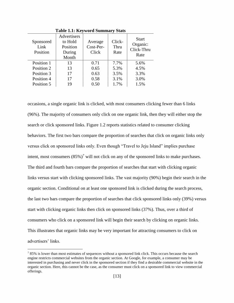
Table 1.1 provides some summary statistics for the five ad positions. Because of the

second-price auction mechanism, an advertiser’s position may change throughout the day as

firms alter their bids. We find that the average number of positions for an advertiser is 2.8 per

day, with a standard deviation 1.3. The second column in Table 1.1 shows that each ad position

has been occupied by many different advertisers. The third column shows that cost-per-click

varies significantly across positions, from about US $0.50 for the 5th position to $0.71 for the top

position. There is also a large variation in these prices. The fourth column shows that the click-

through rate is monotonically declining from the top position (7.7%) to the 5th position (1.7%).

When restricted to those searches that start with clicking at least one organic link, the last

column of the table shows that the click-through rate is also monotonically declining from the

top position (5.6%) to the 5th position (1.5%).

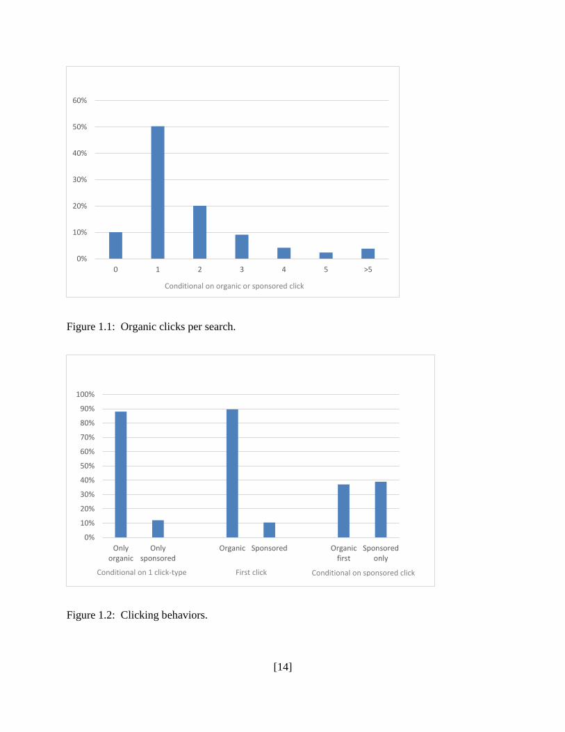
Figure 1.1 provides information on the number of organic links clicked per search,

conditional that at least one sponsored or organic link has been clicked. In 50% of such

[13]

Table 1.1: Keyword Summary Stats

Sponsored

Link

Position

Advertisers

to Hold

Position

During

Month

Average

Cost-Per-

Click

Click-

Thru

Rate

Start

Organic:

Click-Thru

Rate

Position 1 13 0.71 7.7% 5.6%

Position 2 13 0.65 5.3% 4.5%

Position 3 17 0.63 3.5% 3.3%

Position 4 17 0.58 3.1% 3.0%

Position 5 19 0.50 1.7% 1.5%

occasions, a single organic link is clicked, with most consumers clicking fewer than 6 links

(96%). The majority of consumers only click on one organic link, then they will either stop the

search or click sponsored links. Figure 1.2 reports statistics related to consumer clicking

behaviors. The first two bars compare the proportion of searches that click on organic links only

versus click on sponsored links only. Even though “Travel to Jeju Island” implies purchase

intent, most consumers (85%)7 will not click on any of the sponsored links to make purchases.

The third and fourth bars compare the proportion of searches that start with clicking organic

links versus start with clicking sponsored links. The vast majority (90%) begin their search in the

organic section. Conditional on at least one sponsored link is clicked during the search process,

the last two bars compare the proportion of searches that click sponsored links only (39%) versus

start with clicking organic links then click on sponsored links (37%). Thus, over a third of

consumers who click on a sponsored link will begin their search by clicking on organic links.

This illustrates that organic links may be very important for attracting consumers to click on

advertisers’ links.

7 85% is lower than most estimates of sequences without a sponsored link click. This occurs because the search

engine restricts commercial websites from the organic section. At Google, for example, a consumer may be

interested in purchasing and never click in the sponsored section if they find a desirable commercial website in the

organic section. Here, this cannot be the case, as the consumer must click on a sponsored link to view commercial

offerings.

[14]

Figure 1.1: Organic clicks per search.

Figure 1.2: Clicking behaviors.

0%

10%

20%

30%

40%

50%

60%

0 1 2 3 4 5 >5

Conditional on organic or sponsored click

0%

10%

20%

30%

40%

50%

60%

70%

80%

90%

100%

Onlyorganic

Onlysponsored

Organic Sponsored Organicfirst

Sponsoredonly

Conditional on sponsored clickConditional on 1 click-type First click

[15]

Figure 1.3 shows the percentage of consumers who click a sponsored link, conditional on

first clicking a number of organic links. For consumers who only click a single organic link, 10%

will proceed to click a sponsored link. For consumers who click 5 organic links, 24% will

proceed to click a sponsored link. The more organic links a consumer clicks, the more likely that

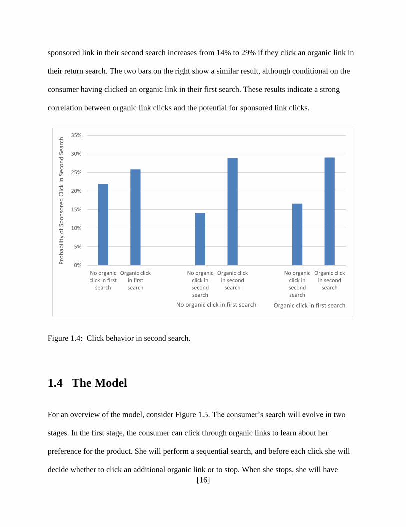
consumer is to click a sponsored link. Now consider consumers who search the keyword, and

then return later to search it again.8 Figure 1.4 provides information on the likelihood that these

consumers will click sponsored links conditional on the organic links that they have clicked

either in the their current search or a previous search. The first two bars indicate that if a

consumer clicked an organic link in their first search, their likelihood of clicking a sponsored

Figure 1.3: Sponsored clicks after organic clicks.

link in their second search increases from 22% to 26%. The two middle bars indicate that if a

consumer did not click an organic link in their first search, then their likelihood of clicking a

8 50% of repeat searchers do so within an hour and half, 93.2% do so within a week. For the following statistics, and

later analysis with repeat searchers, we remove consumers who began their search either within the first or last week

of the observation period.

0%

5%

10%

15%

20%

25%

1 2 3 4 5

Pro

bab

ility

use

r cl

icks

sp

on

sore

d li

nk

Organic link clicks to start search sequence

[16]

sponsored link in their second search increases from 14% to 29% if they click an organic link in

their return search. The two bars on the right show a similar result, although conditional on the

consumer having clicked an organic link in their first search. These results indicate a strong

correlation between organic link clicks and the potential for sponsored link clicks.

Figure 1.4: Click behavior in second search.

1.4 The Model

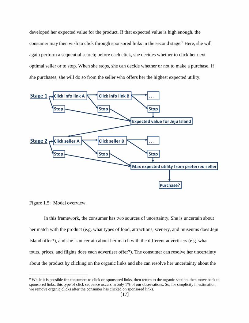
For an overview of the model, consider Figure 1.5. The consumer’s search will evolve in two

stages. In the first stage, the consumer can click through organic links to learn about her

preference for the product. She will perform a sequential search, and before each click she will

decide whether to click an additional organic link or to stop. When she stops, she will have

0%

5%

10%

15%

20%

25%

30%

35%

No organicclick in first

search

Organic clickin firstsearch

No organicclick insecondsearch

Organic clickin second

search

No organicclick insecondsearch

Organic clickin second

search

Pro

bab

ility

of

Spo

nso

red

Clic

k in

Sec

on

d S

earc

h

No organic click in first search Organic click in first search

[17]

developed her expected value for the product. If that expected value is high enough, the

consumer may then wish to click through sponsored links in the second stage.9 Here, she will

again perform a sequential search; before each click, she decides whether to click her next

optimal seller or to stop. When she stops, she can decide whether or not to make a purchase. If

she purchases, she will do so from the seller who offers her the highest expected utility.

Figure 1.5: Model overview.

In this framework, the consumer has two sources of uncertainty. She is uncertain about

her match with the product (e.g. what types of food, attractions, scenery, and museums does Jeju

Island offer?), and she is uncertain about her match with the different advertisers (e.g. what

tours, prices, and flights does each advertiser offer?). The consumer can resolve her uncertainty

about the product by clicking on the organic links and she can resolve her uncertainty about the

9 While it is possible for consumers to click on sponsored links, then return to the organic section, then move back to

sponsored links, this type of click sequence occurs in only 1% of our observations. So, for simplicity in estimation,

we remove organic clicks after the consumer has clicked on sponsored links.

Stage 1 Click info link A Click info link B . . .

Stop Stop Stop

Expected value for Jeju Island

Stage 2 Click seller A Click seller B . . .

Stop Stop Stop

Max expected utility from preferred seller

Purchase?

[18]

advertisers by clicking on the sponsored links. This framework will apply to any keyword in

which consumers have these two sources of uncertainty (e.g. experience goods, fashion goods,

technological products, etc.); more generally, it will also apply to any purchase decision in which

the consumer is uncertain about whether to purchase from the general product category and has

the ability to search for product information prior to deciding from which seller to purchase (e.g.

cars, smart phones, new homes, etc.).

We assume that consumer i’s utility for buying from an advertiser at ad position j in the

sponsored link section (advertiser j), Uij, is the following:

Uij = 𝑞𝑖∗ + 𝜐𝑖𝑗 (1.1)

where 𝑞𝑖∗ is the (true) value for the consumer that is associated with the “product.” In our

example, the attributes associated with a trip to Jeju Island constitute the product. The product

preference represents what a consumer can expect to experience when making a purchase from

an advertiser. This is heterogeneous across individuals since the product (Jeju Island) has

attributes that appeal differently to different people (i.e. it may be an ideal vacation place for

families but not so for couples). We assume that 𝑞𝑖∗ is common for all advertisers. The consumer

may only have limited prior knowledge regarding this value but she can obtain more product

attribute information by browsing web pages linked from the organic results section. We assume

that 𝑞𝑖∗ ~𝑁(�̅�, 𝜎𝑞

2) across all consumers who search for the keyword.10

By purchasing (e.g. buying a tour package) from advertiser j, the consumer will obtain a

match value 𝜐𝑖𝑗 that is individual- and advertiser-specific. 𝜐𝑖𝑗 represents how the advertiser’s

10 We do not model the choice of keyword, so the distribution of qi* represents the population distribution

conditional on having chosen to search the keyword.

[19]

offering differs from the consumer’s expectation about a purchase of a product (𝑞𝑖∗). We specify

the match value as

𝜐𝑖𝑗 = 𝜇𝑖𝑗 + 𝜉𝑗 + 𝑒𝑖𝑗 (1.2)

where 𝜇𝑖𝑗~𝑁(0, 𝜎𝜇2) is the consumer’s preference for advertiser j’s offering that is known prior

to clicking on j’s sponsored link.11 This represents the consumer’s partial knowledge about what

advertiser j may offer (e.g. prior knowledge about prices or flights). Also, the consumer may

have a specific preference for the advertiser if she has previously purchased from the firm. 𝜉𝑗

represents the average match value across all consumers, and 𝑒𝑖𝑗~𝑁(0, 𝜎𝑒2) measures the

individual-specific match value of the advertiser’s offering. The former captures the advertiser’s

average match value (i.e. pricing, quality of service, quality of hotels, and travel options with

regard to a Jeju Island tour at the time of search), and the latter captures how the offering

matches with the consumer's specific needs (i.e. prices of packages at the time at which the

consumer would like to travel, the timing of the available flights relative to the consumer’s

preferred flight times). Both components are unknown to the consumer and will only be revealed

after the consumer clicks on the sponsored link to browse the advertiser’s website.

If the consumer chooses not to buy from any of the advertisers, we normalize the utility

of the outside option to be 0. For “Travel to Jeju Island,” the outside option may include

traveling to a different destination (thus the consumer may search other travel-related keywords)

or opting not to travel.

11 We assume 𝜇𝑖𝑗 to be mean 0 for computational simplicity. This is a fragmented market with many small travel

agencies. Without this assumption, bidding equilibriums become unclear, and it is not clear what will be gained

substantially.

[20]

1.4.1 Consumer Learning

1.4.1.1 Prior Beliefs and Learning from Organic Results

We assume that, prior to keyword search, the consumer has a prior belief about her own 𝑞𝑖∗, 𝑞𝑖

0.

We assume that this prior belief across all consumers is distributed as

𝑞𝑖0 ~ N(�̅�, 𝜎0

2) (1.3)

where �̅� is the (true) average value across all consumers, 𝜎02 is the variance in prior beliefs across

consumers, and 𝑞𝑖0 is constructed from i’s prior information about the product. This assumption

implies that consumers are not systematically biased in prior beliefs. The consumer understands

that, because of limited information, her prior belief may be incorrect; therefore, her perceived

value for 𝑞𝑖∗ is modeled as

𝑞𝑖∗ ~𝑁(𝑞𝑖

0, 𝜎12) (1.4)

where 𝜎12 captures the magnitude of the consumer’s initial uncertainty.12

This modeling construction implies that

𝜎𝑞2 = 𝜎0

2 + 𝜎12

We assume 𝜎02 < 𝜎𝑞

2 because prior preferences based on limited information should be more

concentrated than the true heterogeneity. In the example of Jeju Island, most consumers have

heard that the island is a fun place to visit, so their prior beliefs may be similar with each other.

12 We assume 𝜎1

2 to be common to all consumers. We do not have the data to identify heterogeneity in uncertainty of

initial product preference, so we make a reasonable assumption. This assumption will not alter the substantial results

unless some correlation between level of uncertainty and 𝑞𝑖0 exists.

[21]

However, there are many things that the island offers (e.g. weather, food, activities, expenditures

etc.) that some visitors may love and some visitors may dislike. The dispersion of true

preferences therefore should have larger variance than the dispersion of prior beliefs. With this

setup, prior beliefs and true preferences are positively correlated, i.e., cov(qi0, qi*) > 0, which we

believe is a reasonable assumption as the consumers have some sense of the product prior to

clicking organic links.

With each organic click, the consumer receives information about her true value, via

pictures, blogs, reviews, informative websites, etc.13 This informs her about 𝑞𝑖∗. Suppose the

consumer clicks on an organic link k and browses the web page. We assume that she will receive

a signal about 𝑞𝑖∗. The signal is distributed as follows

Sik ~ N(𝑞𝑖∗, 𝜎𝑠

2) (1.5)

where 𝜎𝑠2 represents the magnitude of the noise from the signal. As no website can fully reveal

every attribute of the product, the information that the consumer obtains will never be perfect;

however, as long as there is no systematic bias from organic results, clicking more organic links

will reduce the consumer’s uncertainty, and her updated belief will converge to the true 𝑞𝑖∗.

We assume that the consumer knows 𝜎12 and 𝜎𝑠

2, and updates her belief in a Bayesian

manor. The updating process is similar to Erdem and Keane (1996), although in this process the

consumer is learning about her true individual preference for the product rather than about the

mean preference of the population, q̅. After clicking K1 organic links, the updated belief will be

13 The links may either include information about Jeju Island, or information about “travel” to Jeju Island which can

inform the consumer about the general costs, difficulties, airlines, and alternative travels options, along with tips and

tricks for travelers. In our data, nearly every organic link relates to information about Jeju Island, as opposed to the

“travel” information.

[22]

𝑞𝑖∗ ~𝑁(𝑞𝑖,𝐾1, 𝜎1,𝐾1

2 ) (1.6)

where

𝑞𝑖,𝐾1 = 𝑞𝑖,𝐾1−1 + 𝜎1,𝐾1

2

𝜎1,𝐾12 +𝜎𝑠

2 (Sik - 𝑞𝑖,𝐾1−1) (1.7)

and

𝜎1,𝐾12 =

11

𝜎12 +

𝐾1

𝜎𝑠2

(1.8)

Notice that 𝜎1,𝐾12 evolves deterministically with each click, and the distribution of potential

signals from the i’s perspective at any click, 𝜎𝜔2 , is given by

𝜎𝜔2 ~ N(𝑞𝑖,𝐾1, 𝜎1,𝐾1

2 + 𝜎𝑠2) (1.9)

1.4.1.2 Prior Beliefs and Learning from Sponsored Links

The consumer is also uncertain about how the advertisers’ offerings match with her specific

needs and preferences. This uncertainty involves 𝜉𝑗 and 𝑒𝑖𝑗 from equation (1.2). The advertisers

are ranked in the sponsored section, and this ranking was endogenously determined by the

bidding strategy of the advertisers. Thus the ranking may provide information to the consumer.

We adopt the signaling theory, applied to the search advertising context, to model the

consumer’s prior belief of the average match value 𝜉𝑗. Consistent with Athey and Ellison (2011)

and Chen and He (2011), we assume firm bids are increasing in average match value, 𝜉𝑗.

Therefore firms are ranked according to average match value, as we assume that 𝜇𝑖𝑗, the

consumer preference for advertiser j prior to clicking any sponsored links, is averaged at 0 across

consumers. Thus, in aggregate, no advertiser has an advantage in generating sales over the others

[23]

if consumers are not informed about 𝜉𝑗. The incentive of signaling if the advertiser has a high 𝜉𝑗

will be strong. Our model setup therefore is consistent with the necessary conditions for the

signaling theory to work. Bentley et al. (2014) provide significant empirical evidence supporting

this theory. They find that advertisers with higher average match values bid more for better

positions and will increase their bids when their match value increases. Furthermore, consumers

can infer this strategy and are more likely to click higher-ranked links.

To model search with ranking information, we adopt the “ranked search” model (Bentley

et al. 2015) to model the situation in which consumers can search through a list of options which

have been ranked according to average consumer preferences. We assume that each of 5

advertisers receives a draw of 𝜉𝑗 from the N(0,1) distribution. Based on these 𝜉′𝑠, advertisers

place their bids. Advertisers are then ordered, in position, by their bids; the one with the highest

𝜉 obtains the top position and so forth. We assume that the consumer can rationally infer the

advertisers’ bidding strategy and the outcomes. Although she cannot observe the bid amount

from each advertiser, she will form her prior beliefs about 𝜉′𝑠 based on ad positions. Let 𝑃𝑖 =

{𝑃𝑖1, … , 𝑃𝑖5} be the collection of the ad positions of the five advertisers. The prior expectation of

𝜉𝑗 for the advertiser at the j-th position can be derived from order statistics

𝐸[𝜉𝑗|𝜉1 ≥ ⋯ ≥ 𝜉𝑗 ≥ ⋯ ≥ 𝜉5] (1.10)

with the prior variance denoted as 𝜎𝑗,02 ≡ 𝑣𝑎𝑟(𝜉𝑗|𝜉1 ≥ ⋯ ≥ 𝜉𝑗 ≥ ⋯ ≥ 𝜉5).

Upon clicking a link at the k-th position, 𝜉𝑘 (and eik, see equation (1.2)) is revealed. The

consumer will update her belief of 𝜉𝑗 , j ≠ k. If the j-th position is higher than the k-th position, the

updated expected 𝜉𝑗 is

[24]

𝐸[𝜉𝑗|𝜉1 ≥ ⋯ ≥ 𝜉𝑗 ≥ ⋯ ≥ 𝜉𝑘−1 ≥ 𝜉𝑘, 𝜉𝑘] (1.11’)

That is, given 𝜉𝑘, the consumer will form an expectation conditional on the order

relationship 𝜉1 ≥ ⋯ ≥ 𝜉𝑗 ≥ ⋯ ≥ 𝜉𝑘−1 ≥ 𝜉𝑘. Likewise, if the j-th position is lower than the k-th

position, the updated expected 𝜉𝑗 is

𝐸[𝜉𝑗|𝜉𝑘 ≥ ⋯ ≥ 𝜉𝑗 ≥ ⋯ ≥ 𝜉5, 𝜉𝑘] (1.11”)

The variance for 𝜉𝑗 will be updated correspondingly. The above updating equations suggest that,

given 𝜉𝑘, the distribution of 𝜉𝑗 is truncated either from below (if the j-th position is higher than

the k-th position) or from above (if the j-th position is lower than the k-th position), and the

consumer expectation of 𝜉𝑗 and its variance are derived from such a truncated distribution that

also takes account of the order relationship of 𝜉′𝑠 that have not been revealed. If the consumer

has clicked more than one link, she will update her expectation and variance in a similar manner.

Let’s consider an example to highlight this updating. Say the consumer expects prices for

a Jeju tour to be around $2,000, and let price be the only attribute constituting average match

value. So she clicks on the top-ranked firm, expecting it to offer the best price, but she sees that

prices are closer to $4,000. Given that this firm is the top-ranked advertiser, it is unlikely that the

lower-ranked firms are priced so much lower, at around $2,000. These firms are likely to be

priced closer to $4,000, or above, so the consumer will update her expectations. In a standard

search model, we would have to impose that the consumer does not update her expectations and

still expects advertisers to be priced at $2,000, regardless of what is learned in her first click. In a

“ranked search” context, this assumption would be wrong.

[25]

The updated expectations and variances, under the normal distribution assumption for

𝜉′𝑠, do not have a closed-form expression. In model estimation, we rely on the simulation

method to calculate the updated beliefs. More details will be provided in the model estimation

section.

1.4.2 Two-Stage Information Search

The consumer information search process evolves in two stages. In the first stage, the consumer

optimally searches in the organic section to learn about the product, and thus her true preference

𝑞𝑖∗. We assume that there is a constant marginal cost of clicking an organic link and browsing the

web page, 𝑐𝑜𝑟𝑔. With each click at an organic link, the consumer can decide to either click an

additional organic link and remain in the first stage search, or move to the second stage of

search. If the consumer moves to the second stage, she will have developed her expected

preference for the product. In the second stage, she will decide to either stop the search and leave

the search results page (in which case there will be no purchase from any advertisers), or to

sequentially choose sponsored links to click for the opportunity to purchase from the advertisers.

Suppose she has clicked K2 sponsored links and the 𝜉’s and e’s of those links are revealed. She

may leave the search results page (so no purchase will be made), or return to purchase from one

of the links that have been clicked which brings her the highest expected utility, depending on

which choice has higher expected value. If she has not clicked all sponsored links, she can also

choose to click an additional sponsored link for the opportunity to find a better match. We

assume that there is another constant marginal cost of clicking a sponsored link and browsing the

commercial website, 𝑐𝑠𝑝𝑜𝑛.

[26]

We allow corg to differ from cspon. The cost of clicking represents the net of the utility and

disutility components for each click. For organic clicks, there is a disutility of time, but there

may also be a positive utility from reading stories regarding vacation activities or traveling

experience or enjoying beautiful pictures of the island. Conversely, browsing a commercial

website can be a different experience. The time spent on organizing exactly what time to get a

flight to and from the island, to weigh the cost of a layover, and to compare prices etc. can be

tedious and longer. In data, the median time spent on an organic click is 89 seconds, and 117

seconds on a sponsored click. The consumer must also consider how much money they are

willing to spend on a flight/hotel/car rental, etc. It may take more cognitive resources to

complete those tasks. We thus expect the cost of a sponsored click to be greater than the cost of

an organic click.

In the remaining part of this section, we will develop the dynamic search model in which

the consumer will optimally search for the product-related information and advertiser-specific

information in the two stages.

1.4.2.1 First Stage - Organic Clicks

In the first stage, the consumer can resolve her uncertainty about the product. After clicking K1

organic links in the first stage, the consumer obtains K1 signals and her updated belief will be

𝑞𝑖∗ ~𝑁(𝑞𝑖,𝐾1, 𝜎1,𝐾1

2 ) (see equations (6) to (8)).14 Let 𝝁𝑖 = {𝜇𝑖1, … , 𝜇𝑖5} be the collection of the

consumer’s known preferences for the five advertisers from the top to the lowest position. The

14 K1 can be zero. In which case, the consumer does not have any new information and only holds the prior belief.

That is, 𝑞𝑖,𝐾1 = 𝑞𝑖0 and 𝜎1,𝐾1

2 = 𝜎12.

[27]

state variables that will determine the optimal search strategy in the first stage, include 𝑋𝑖,𝐾1 =

{𝑞𝑖,𝐾1, 𝜎1,𝐾12 , 𝝁𝑖}.

Let 𝑍𝑖0 = {𝑞𝑖,𝐾1, 𝝁𝑖}. This is the set of state variables that determine the search strategy

when the second stage search at the sponsored links section (details are below) starts. Let

𝑉(𝑞𝑖,𝐾1, 𝝁𝑖) represents the expected value of the consumer when she adopts the optimal search

rule in the second stage. The transition of the state variables 𝑋𝑖,𝐾1 with the (K1+1)th search is as

follows: 𝝁𝑖 remains unchanged and 𝜎1,𝐾1+12 will evolve deterministically via equation (1.8). The

only stochastic component in the state variables is 𝑞𝑖,𝐾1+1, which transitions depending on the

signal Si,K1+1 with the distribution function in equation (1.5). Conditional on Si,K1+1, 𝑞𝑖,𝐾1+1 will

evolve via equation (1.7). The expected value of an additional search in the organic section,

conditional on 𝑞𝑖,𝐾1 and 𝝁𝑖, can be written as

𝐸𝑉𝐾1+1(𝑞𝑖,𝐾1, 𝝁𝑖) = ∫ max {𝑉(𝑞𝑖,𝐾1+1, 𝝁𝑖), 𝐸𝑉𝐾1+2(𝑞𝑖,𝐾1+1, 𝝁𝑖) − 𝑐𝑜𝑟𝑔} 𝑑𝐹(𝑆𝑖,𝐾1+1) (1.12)

Thus, the consumer’s value function in the first stage is

𝑊𝐾(𝑞𝑖,𝐾1, 𝝁𝑖) = max {𝑉(𝑞𝑖,𝐾1, 𝝁𝑖), 𝐸𝑉𝐾1+1(𝑞𝑖,𝐾1, 𝝁𝑖) − 𝑐𝑜𝑟𝑔} (1.13)

As the additional search incurs cost corg, the consumer will stop first stage search if and

only if

𝑉(𝑞𝑖,𝐾1, 𝝁𝑖) ≥ 𝐸𝑉𝐾1+1(𝑞𝑖,𝐾1, 𝝁𝑖) − 𝑐𝑜𝑟𝑔 (1.14)

Otherwise she will continue to click on the (K1+1)th organic link.

Equation (1.1) implies that the consumer is risk neutral and her objective of information

search is to maximize her expected utility. However, if the consumer has a relatively low prior

[28]

belief 𝑞𝑖0 so that her prior expectation of Uij (see equation (1.1)) is negative, it may be still

optimal to conduct keyword search and click on organic links. The reason is that she always has

the outside option valued at 0. Since she has uncertainty about her true 𝑞𝑖∗, there is a positive

probability that the true value is high enough to make Uij positive for at least one of the

advertisers. She can learn 𝑞𝑖∗ by clicking organic links. If she receives a positive signal, perhaps

by seeing beautiful pictures of the island or reading favorable reviews, she will update her belief

of 𝑞𝑖∗. Given the updated belief, it may become optimal for the consumer to click on sponsored

links, as there is now a greater likelihood that the revealed Uij will become positive. It may also

be optimal for the consumer to click organic links even if she would have clicked a sponsored

link without organic links. This is because there is a positive probability that highest Uij among

all advertisers is actually negative. Therefore, it may be optimal for her to learn about the true 𝑞𝑖∗

from organic links and, if the updated belief of 𝑞𝑖∗ is low, she can avoid purchasing a product that

would have provided lower utility than her outside option, and she can also save her search costs

(cspon) by not searching any sponsored links.

So, intuitively, why will a consumer click organic links? She can click organic links to

gain information to make better purchase decisions and avoid mistakes. For example, if she was

planning on going to Jamaica instead of Jeju Island, she may learn that she would prefer Jeju to

Jamaica and gain the additional utility of going to a more-preferred destination. Or, if she was

planning on a trip to Jeju, she may learn that she would prefer Jamaica instead and, again, gain

the additional utility of traveling to a more-preferred destination.

[29]

1.4.2.2 Second Stage - Sponsored Clicks

In the second stage, the consumer can resolve her uncertainty regarding the advertisers’

offerings. She has formed her updated expectation of 𝑞𝑖∗, 𝑞𝑖,𝐾1 (see equation (1.7)), in the first

stage. This expectation will not change throughout the second stage information search. In our

Jeju Island example, because the advertisers are travel agencies, it is unlikely that by browsing

their websites the consumer can learn unbiased information about the activities, sight-seeing

places, food, etc. on Jeju Island. Conditional on the state variables 𝑍𝑖0 = {𝑞𝑖,𝐾1, 𝝁𝑖}. and the prior

expectation of 𝜉𝑗, 𝐸[𝜉𝑗|𝜉1 ≥ ⋯ ≥ 𝜉𝑗 ≥ ⋯ ≥ 𝜉5], for each of the advertisers that is derived from

their ad positions, we assume that the consumer will search sponsored links optimally in a

sequential way. After a sponsored link, say, at the kth position is clicked, 𝜉𝑘 and eik are revealed.

State variables will be updated to be 𝑍𝑖1 = {𝑞𝑖,𝐾1, 𝝁𝑖; 𝜉𝑘, 𝑒𝑖𝑘}, which will determine the optimal

search strategy in the next step. The consumer will either click one of the four remaining links,

or terminate the search by one of the two options, buying from advertiser k or choosing the

outside option with value 0. If she chooses to click a remaining link, state variables will be

updated and the next dynamic decision has to be made, similar to the previous step.

The optimal search rule can be computed using backward induction. Given five

advertisers placed at the sponsored links section, we can calculate, after four sponsored links are

clicked and their 𝜉’s and e’s are revealed, the expected value of clicking the last remaining link.

This expected value is derived from the distribution of 𝜉, conditional on the revealed 𝜉’s, and the

distribution of e, of the last link. Given the expected value, we can calculate, after three

sponsored links are clicked, the expected value of clicking either of the two remaining links. The

procedure will repeat in a backward way, until the first step when the consumer has to decide

[30]

which of the five sponsored links should be clicked. Such a procedure, however, is

computationally very intensive. Given that the conditional expectation of 𝜉 (given 𝜉’s from other

ad positions) does not have a closed-form expression, we have to rely on simulation method to

calculate the expected value of clicking a link at every step. The number of simulation draws and

the number of calculations increase exponentially with the number of sponsored links, and make

this backward induction procedure infeasible in our empirical context.

Weitzman (1979) introduces calculating the reservation price for each search alternative

to simplify the optimal search rule. After clicking K2 links, define

𝑈𝑖,𝐾2∗ = max {0, 𝑚𝑎𝑥𝑘∈𝐾2{𝐸𝑈𝑖𝑘}} (1.15)

where for link k that has been clicked,

𝐸𝑈𝑖𝑘 = 𝑞𝑖,𝐾1 + 𝜇𝑖𝑘 + 𝜉𝑘 + 𝑒𝑖𝑘 (1.16)

represents the updated expected utility of buying from the advertiser. “0” inside the outer

brackets represents the outside option value. The consumer will calculate the reservation price

for each remaining link j, Rj, which is the utility level such that the consumer is indifferent

between clicking the link and accepting the reservation price and terminating the search. For an

attractive advertiser either with higher 𝜇 or at a higher ad position, a higher utility level

(reservation price) is required to make the consumer indifferent between clicking and stopping.

Therefore, the advertiser will have a higher reservation price. Under optimal search, Weitzman

(1979) shows that the consumer will click the link with the highest reservation price, say, Rj, if Rj

> 𝑈𝑖,𝐾2∗ ; otherwise the consumer will stop the search and receive 𝑈𝑖,𝐾2

∗ . Suppose the consumer

clicks a remaining link, state variables will be updated and she has to compute the new

[31]

reservations prices for the remaining links. This is because, as 𝜉 of the newly clicked link is

revealed, the distributions of 𝜉’s of the remaining links will change and thus their reservation

prices have to be updated. Similar procedure will iterate until the consumer stops, or all five

sponsored links have already been clicked, at which point the consumer will receive 𝑈𝑖,5∗ , the

alternative with the highest utility level.

Thus the consumer’s value function in the second stage, conditional on advertisers ranked

as R, is as follows

𝑉𝐾2(𝑞𝑖,𝐾1, 𝝁𝑖; 𝜉𝑗 , 𝑒𝑖𝑗 ∀𝑗 ∈ 𝐾2|𝑹) =

max {0 ,𝑚𝑎𝑥

j∈ k2 {𝐸𝑈𝑖𝑗} ,

𝑚𝑎𝑥

j'∉ k2 {𝐸𝑉𝐾2+1(𝑞𝑖,𝐾1, 𝝁𝑖, 𝜉𝑗 , 𝑒𝑖𝑗 ∀𝑗 ∈ 𝐾2+1; 𝜉𝑗′ , 𝑒𝑖𝑗′|𝑹)} − 𝑐𝑠𝑝𝑜𝑛} (1.17)

Before any click, the consumer has three options. If 𝑉𝐾2 = 0, the consumer will stop her

search, accept her outside option, and not make a purchase. If 𝑉𝐾2 =𝑚𝑎𝑥

j∈ k2 {𝐸𝑈𝑖𝑗}, implying

𝑚𝑎𝑥

j∈ k2 {𝐸𝑈𝑖𝑗} > 0, the consumer will stop her search and purchase from the advertiser she has

clicked who offers her highest expected utility. Note that if the consumer has not clicked on a

sponsored link, K2 is the null set and this option will not be available to her. If 𝑉𝐾2 equals the

third term in the brackets, the consumer will continue her search and click the advertisers who

maximizes her forward-looking utility.

There is a caveat when applying such a reservation price rule to our empirical context:

Weitzman (1979) makes the assumption that expected utilities for options are independent.

Therefore, this rule may not be optimal if the expected utilities between sponsored links are

dependent, which is the case for our model. Clicking link j will reveal 𝜉𝑗, and the consumer will

use this information to update the distribution for the 𝜉’s of links that have not been clicked.

[32]

Clicking link j therefore will change the expected utility of clicking other links. Although this

can be an issue, we argue that the reservation price rule can approximate closely the true optimal

search rule. Assume that the reservation price Rj is higher than Rk. The only reason that the

consumer will choose to click link k before link j is if doing so will reveal more information

regarding the 𝜉’s of sponsored links that have not been clicked. However, clicking link j will also

reveal information for other links. The probability that the increased information value of

clicking link k first dominates the difference between Rj and Rk thus should be very small.

Another scenario may occur in which Rj will not be informative about other links (e.g. she is

considering clicking the top link, and she has already clicked the second link), and thus the

consumer will not benefit from revealing information in the same way she would if she clicks Rk.

For Rk to be optimal, it must update a third options Rl such that Rl becomes preferred to Rj, and is

still optimal to click conditional on Rk, often enough to outweigh the myopic disutility of

choosing Rk before Rj. This is an unlikely scenario.

To investigate whether the reservation price rule is a good approximation of the optimal

dynamic decision rule, we simulate the consumer search behavior under both rules, using the

estimated model parameters. We use backward induction method, as discussed above, to

calculate the standard dynamic optimization decisions, we then also calculate decisions using

reservation utilities, and we compare. For computational feasibility, we assume that there are

only three alternatives: two sponsored links and an outside option. We simulate 5,000 click

sequences under both search rules and compare. For the 5,000 simulated click sequences, there is

not a single difference for the simulated clicks under the two search rules. This will not always

be the case, but clearly the reservation utility decision provides a close approximation for the

standard dynamic optimization. Further, the computation using the optimal dynamic search rule

[33]

took more than 2 days (with 2,000 draws per simulation) and increases exponentially with

additional options, while the reservation price rule took only minutes and increases linearly with

additional options. Therefore, the “ranked search” model can be estimated with a large number

of ranks.

1.5 Estimation

In this section we detail the approach to estimating our model parameters 𝚯 =

{𝜎𝜇, 𝜎𝑒 , 𝜎0, 𝜎1, 𝜎𝑠, 𝑞,̅ 𝑐𝑜𝑟𝑔, 𝑐𝑠𝑝𝑜𝑛}. Note that for identification we normalize 𝜎𝜉 to 1. We use the

simulated likelihood approach to evaluate the likelihood of observed click sequences 𝑛𝑖𝑜, the

number of organic links that have been clicked, and 𝑦𝑖𝑠, the sequence of sponsored links that

have been clicked, in model estimation. We will then discuss the model identification issue in

this section.

1.5.1 Model Estimation

Let N be the total number of searches in data. We obtain our estimated parameters by

maximizing the likelihood function:

�̂� = 𝑎𝑟𝑔𝑚𝑎𝑥 ∏ 𝑃𝑟(𝑛𝑖𝑜, 𝑦𝑖

𝑠|𝚯)𝑁𝑖=1 (1.18)

In the first step, we have to evaluate 𝑉(𝑞𝑖, 𝝁𝑖), the expected value for the consumer when

she adopts the optimal search rule in the second stage, conditional on her updated expectation of

her product preference 𝑞𝑖∗ and preferences for the five advertisers at the sponsored links section,

[34]

𝝁𝑖. This calculation is related to the optimal reservation price rule used in the search in the

second stage. To do so, we use the following procedures: conditional on a trial 𝚯, we

(i) draw 𝑞𝑖𝑠𝑖𝑚 by discretizing a large state space for admissible 𝑞𝑖, and draw 𝜇𝑖𝑗

𝑠𝑖𝑚 for

each advertiser;

(ii) draw 𝜉𝑗𝑠𝑖𝑚 for each advertiser from their distributions of ’s conditional on the ad

position. After the consumer clicks sponsored link j, draw 𝜉𝑗𝑠𝑖𝑚 and 𝑒𝑖𝑗

𝑠𝑖𝑚 that are

revealed to the consumer. Conditional on 𝜉𝑗𝑠𝑖𝑚 and ad positions of all advertisers, then

draw 𝜉𝑘𝑠𝑖𝑚 for other advertisers whose links have not been clicked based on the

distribution. Repeat the simulations in every step after a sponsored link is clicked;

In every step, calculate reservation prices for the remaining sponsored links using the Weitzman

(1979) algorithm, based on 𝑞𝑖𝑠𝑖𝑚, 𝜇𝑖𝑗

𝑠𝑖𝑚, 𝜉𝑗𝑠𝑖𝑚 and 𝑒𝑖𝑗

𝑠𝑖𝑚. Compute the optimal search strategy

before each click. Then calculate 𝑉(𝑞𝑖𝑠𝑖𝑚, 𝜇𝑖

𝑠𝑖𝑚) by averaging over all simulated 𝑈𝑖,𝐾2∗ − 𝑐𝑠𝑝𝑜𝑛 ∗

𝐾2 (𝑈𝑖,𝐾2∗ from equation 1.14). We then use polynomial approximation method to compute V for

other values of q’s and ’s. This gives us the expected value in the second stage, conditional on

𝑞𝑖 and 𝝁𝑖.

In the second step, we backward induct the value of informational organic link clicks,

conditional on 𝑉(𝑞𝑖𝑠𝑖𝑚, 𝜇𝑖

𝑠𝑖𝑚). First, beginning with the last click in our backward induction, we

draw 𝑞𝑖,𝑘𝑠𝑖𝑚 by discretizing a large state space for admissible 𝑞𝑖,𝑘, for each 𝜇𝑖

𝑠𝑖𝑚. Next, we take

draws from the distribution of potential signals from organic results, 𝑆𝑖𝑘𝑠𝑖𝑚, from equation (1.9)

and update 𝑞𝑖,𝑘. We then calculate the updated belief 𝑞𝑖,𝑘+1𝑠𝑖𝑚 using the Bayesian rule. For a given

[35]

draw, the value of clicking an organic link, 𝑉𝑖,𝑘𝑖𝑛𝑓𝑜,𝑑𝑟𝑎𝑤

(𝑞𝑖,𝑘𝑠𝑖𝑚, 𝜇𝑖

𝑠𝑖𝑚), at organic click number k,

is calculated as

𝑉𝑖,𝑘𝑖𝑛𝑓𝑜,𝑑𝑟𝑎𝑤


𝑠𝑖𝑚) (1.19)

= 𝑉(𝑞𝑖,𝑘+1𝑠𝑖𝑚 , 𝜇𝑖

𝑠𝑖𝑚) − 𝑉(𝑞𝑖,𝑘𝑠𝑖𝑚, 𝜇𝑖

𝑠𝑖𝑚) + 𝑉𝑖,𝑘+1𝑖𝑛𝑓𝑜

(𝑞𝑖,𝑘+1𝑠𝑖𝑚 , 𝜇𝑖

𝑠𝑖𝑚)

where 𝑉(𝑞𝑖,𝑘+1𝑠𝑖𝑚 , 𝜇𝑖

𝑠𝑖𝑚) − 𝑉(𝑞𝑖,𝑘𝑠𝑖𝑚, 𝜇𝑖

𝑠𝑖𝑚) is the change in expected value in the second-stage as

the consumers belief is updated to 𝑞𝑖,𝑘+1𝑠𝑖𝑚 , and 𝑉𝑖,𝑘+1

𝑖𝑛𝑓𝑜(𝑞𝑖,𝑘+1

𝑠𝑖𝑚 , 𝜇𝑖𝑠𝑖𝑚) is the option value of

continuing to click organic links. 𝑉𝑖,𝑘+1𝑖𝑛𝑓𝑜

(𝑞𝑖,𝑘+1𝑠𝑖𝑚 , 𝜇𝑖

𝑠𝑖𝑚) = 0 for the last click in the backward

induction. For each 𝜇𝑖𝑠𝑖𝑚, we can now linearly interpolate the value of clicking an additional

organic link at each click k, conditional on 𝑞𝑖,𝑘 and 𝝁𝑖.

In the third step, we simulate consumer clicks in the first stage, conditional on 𝑉𝑖,𝑘𝑖𝑛𝑓𝑜

derived in the second estimation step. Then, we derive probabilities of click sequences in the

second stage, conditional on the updated 𝑞𝑖𝑠𝑖𝑚 from the first stage, in a similar manner to the first

estimation step.

First, we draw prior beliefs 𝑞𝑖0,𝑠𝑖𝑚

and, after interpolating 𝑉𝑖,𝑘𝑖𝑛𝑓𝑜

, determine whether an

organic link is clicked or not. If organic link k is clicked, the consumer receives a signal from the

organic result, 𝑆𝑖𝑘𝑠𝑖𝑚. We then calculate the updated belief 𝑞𝑖

𝑠𝑖𝑚 using the Bayesian rule. After

each organic link is clicked, the consumer will decide whether to continue clicking organic links

or move to the second stage search, based on 𝑉𝑖,𝑘𝑖𝑛𝑓𝑜


𝑠𝑖𝑚). This simulation gives us the

simulated number of organic clicks, 𝑛𝑖𝑜,𝑠𝑖𝑚

, and each consumer’s updated 𝑞𝑖𝑠𝑖𝑚.

[36]

For each simulation, we use the updated 𝑞𝑖𝑠𝑖𝑚, from the first stage, for the second stage

calculations. Similar to the above procedure (step 1), we draw 𝜉𝑗𝑠𝑖𝑚 based on the ad positions

and, after each sponsored links is clicked, we draw 𝜉𝑘𝑠𝑖𝑚for remaining sponsored links. We then

use the reservation price rule again to simulate the optimal sponsored clicks, 𝑦𝑖𝑠𝑖𝑚. Given that

there is a large number of possible sequences of sponsored clicks (120 altogether), the number of

simulations required to reliably evaluate the likelihood of a specific 𝑦𝑖𝑠 is exceedingly high and

poses a computational challenge in the model estimation. We choose to use a scaled multivariate

logistic CDF to smooth the clicking probabilities (McFadden 1989). Similar procedure is also

adopted in Honka et al (2014). After K2 sponsored links are clicked, the probability of choosing

to click one of the remaining sponsored links is a function of its reservation price Rj, the

reservation prices of other remaining links Rk, and 𝑈𝑖,𝐾2∗ (see equation (1.15)). The probability of

clicking link j is specified as

𝑃𝑟(𝑐𝑙𝑖𝑐𝑘𝑖𝑛𝑔 𝑗) =𝑒𝑥𝑝(𝑅𝑗 𝜎⁄ )

∑ 𝑒𝑥𝑝(𝑅𝑘 𝜎⁄ )𝑘 𝑛𝑜𝑡 𝑏𝑒𝑒𝑛 𝑐𝑙𝑖𝑐𝑘𝑒𝑑 +𝑒𝑥𝑝(𝑈𝑖,𝐾2∗ 𝜎⁄ )

(1.20)

We fixed the scaling parameter to be 0.025, small enough so that the smoothed

probability function can approximate well the discrete clicking choice. Based on this probability

we can calculate the probability for each observed 𝑦𝑖𝑠, denoted as 𝑃𝑟𝑠𝑖𝑚(𝑦𝑖

𝑠|𝑞𝑖𝑠𝑖𝑚). The

probability of 𝑦𝑖𝑠 is calculated as

𝑃𝑟(𝑦𝑖𝑠|𝑛𝑖

𝑜) = 𝑃𝑟𝑠𝑖𝑚(𝑗|𝑞𝑖𝑠𝑖𝑚) ∗ 𝑃𝑟𝑠𝑖𝑚(𝑙|𝑐𝑙𝑖𝑐𝑘𝑒𝑑 𝑗, 𝑞𝑖

𝑠𝑖𝑚) ∗

𝑃𝑟𝑠𝑖𝑚(ℎ|𝑐𝑙𝑖𝑐𝑘𝑒𝑑 𝑙 𝑎𝑛𝑑 𝑗, 𝑞𝑖𝑠𝑖𝑚) … (1.21)

By repeating the procedures for NS times, we can calculate the probability for the observed

number of organic clicks, 𝑛𝑖𝑜, and click sequence, 𝑦𝑖

𝑠, as the following:

[37]

𝑃𝑟(𝑛𝑖𝑜 , 𝑦𝑖

𝑠|𝚯) =1

𝑁𝑆∑ {𝑛𝑖

𝑜,𝑠𝑖𝑚 = 𝑛𝑖𝑜}𝑁𝑆

𝑠𝑖𝑚=1 ∗ 𝑃𝑟(𝑦𝑖𝑠|𝑛𝑖

𝑜) (1.22)

We iterate the model parameters 𝚯 until the likelihood function in equation (1.18) is

maximized.

1.5.2 Identification

In this section, we discuss how the model parameters are identified from the data. Given that we

only observe the sequence of organic and sponsored clicks, there are several identification

assumptions made in the model. First, we assume that the mean of the prior beliefs across

consumers is consistent with the mean product preference, �̅�, in the population. Therefore, there

is no persistent bias in consumers’ prior beliefs about their preference for the product. We also

assume that the signals from organic results are unbiased with the mean equal to the true 𝑞𝑖∗ of

each consumer. This is a weaker assumption as we can assume that if signals intend to be biased,

the consumers can filter through the bias to reveal the true signal. We will test how our results

are robust to these assumptions later in the paper.

We begin by discussing the parameters associated with organic link clicks. The mean

preference for the keyword, �̅�, and the variance in the distribution of prior mean beliefs across

the population, 𝜎0, are identified by the percentage of consumers who first click sponsored links,

first click organic links, or choose not to click. From our model, we have 3 moments to identify

these 2 parameters: P(first click sponsored), P(first click organic), and P(no clicks) = 1 - P(first

click sponsored) - P(first click organic). A high �̅� and low 𝜎0 will lead most consumers to click

sponsored links only. A high �̅� and high 𝜎0 will lead many consumers to click sponsored links,

but a portion will start with organic links and a smaller portion will click nothing at all. A low �̅�

[38]

and low 𝜎0 implies that most consumers to start with organic links. And a low �̅� and high 𝜎0

implies many consumers will start with organic links and a portion will start with sponsored

links and a portion will click nothing at all.

The effects of the signal noise, 𝜎𝑠, and the marginal cost of clicking organic clicks, corg,

are similar. A low 𝜎𝑠 will incentivize organic clicks, as i will gain a lot of information with each

click, while a low corg will also incentivize organic clicks. But note that a low 𝜎𝑠 will also lead to

diminishing returns for organic clicks as the consumers’ uncertainty will shrink with each click,

disincentivizing organic clicks as the consumer clicks more links. The two parameters are

identified by the average number of organic links clicked and the distribution of the number of

organic links clicked. From the model, we have 5 moments to identify these 2 parameters, each

conditional on the consumer having clicked an organic link: P(1 organic click), P(2 organic

clicks), P(3 organic clicks), P(4 organic clicks), P(more than 4 organic clicks).

The consumer’s initial uncertainty about their preference for the product, 𝜎1, is identified

by the proportion of consumers who click sponsored links after having clicked organic links. We

have 5 moments to identify this parameter: P(sponsored click | 1 organic click), P(sponsored

click | 2 organic clicks), P(sponsored click | 3 organic clicks), P(sponsored click | 4 organic

clicks), P(sponsored click | more than 4 organic clicks). If �̅� is negative, then each of these

probabilities will be larger if 𝜎1 is large. Because 𝜎𝑞2 = 𝜎0

2 + 𝜎12, if 𝜎1 is larger, 𝜎𝑞 is larger and

a larger portion of the consumers will have a positive true preference for the product, which they

learn from organic clicks. Conversely if �̅� is positive, the opposite is true, and we would expect

to see fewer sponsored clicks after organic clicks.

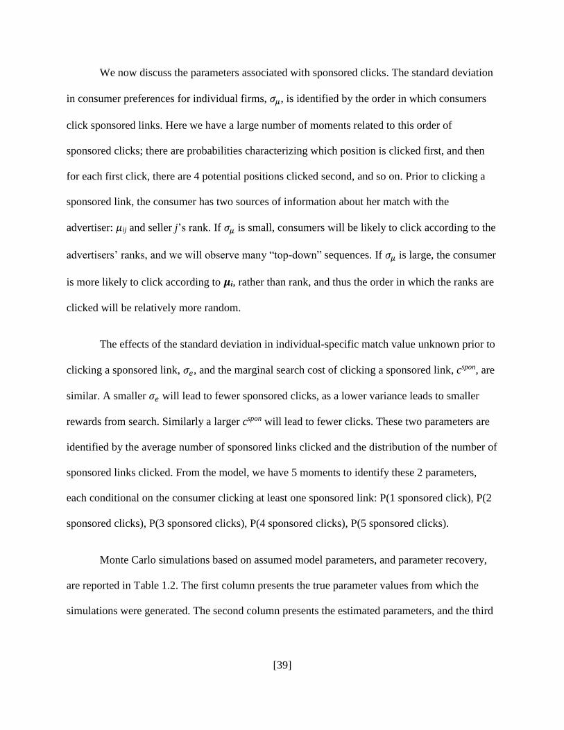
[39]

We now discuss the parameters associated with sponsored clicks. The standard deviation

in consumer preferences for individual firms, 𝜎𝜇, is identified by the order in which consumers

click sponsored links. Here we have a large number of moments related to this order of

sponsored clicks; there are probabilities characterizing which position is clicked first, and then

for each first click, there are 4 potential positions clicked second, and so on. Prior to clicking a

sponsored link, the consumer has two sources of information about her match with the

advertiser: 𝜇ij and seller j’s rank. If 𝜎𝜇 is small, consumers will be likely to click according to the

advertisers’ ranks, and we will observe many “top-down” sequences. If 𝜎𝜇 is large, the consumer

is more likely to click according to 𝝁i, rather than rank, and thus the order in which the ranks are

clicked will be relatively more random.

The effects of the standard deviation in individual-specific match value unknown prior to

clicking a sponsored link, 𝜎𝑒, and the marginal search cost of clicking a sponsored link, cspon, are

similar. A smaller 𝜎𝑒 will lead to fewer sponsored clicks, as a lower variance leads to smaller

rewards from search. Similarly a larger cspon will lead to fewer clicks. These two parameters are

identified by the average number of sponsored links clicked and the distribution of the number of

sponsored links clicked. From the model, we have 5 moments to identify these 2 parameters,

each conditional on the consumer clicking at least one sponsored link: P(1 sponsored click), P(2

sponsored clicks), P(3 sponsored clicks), P(4 sponsored clicks), P(5 sponsored clicks).

Monte Carlo simulations based on assumed model parameters, and parameter recovery,

are reported in Table 1.2. The first column presents the true parameter values from which the

simulations were generated. The second column presents the estimated parameters, and the third

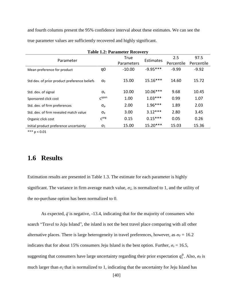
[40]

and fourth columns present the 95% confidence interval about these estimates. We can see the

true parameter values are sufficiently recovered and highly significant.

Table 1.2: Parameter Recovery

Parameter

True Parameters

Estimates 2.5

Percentile 97.5

Percentile

Mean preference for product q̅0 -10.00 -9.95*** -9.99 -9.92

Std dev. of prior product preference beliefs σ0 15.00

15.16*** 14.60 15.72

Std. dev. of signal σs 10.00

10.06*** 9.68 10.45

Sponsored click cost cspon 1.00 1.03*** 0.99 1.07

Std. dev. of firm preferences σµ 2.00 1.96*** 1.89 2.03

Std. dev. of firm revealed match value σe 3.00 3.12*** 2.80 3.45

Organic click cost corg 0.15 0.15*** 0.05 0.26

Initial product preference uncertainty σ1 15.00 15.20*** 15.03 15.36

*** p < 0.01

1.6 Results

Estimation results are presented in Table 1.3. The estimate for each parameter is highly

significant. The variance in firm average match value, σ, is normalized to 1, and the utility of

the no-purchase option has been normalized to 0.

As expected, q̅ is negative, -13.4, indicating that for the majority of consumers who

search “Travel to Jeju Island”, the island is not the best travel place comparing with all other

alternative places. There is large heterogeneity in travel preferences, however, as σ0 = 16.2

indicates that for about 15% consumers Jeju Island is the best option. Further, σs = 16.5,

suggesting that consumers have large uncertainty regarding their prior expectation 𝑞𝑖0. Also, σ0 is

much larger than σ that is normalized to 1, indicating that the uncertainty for Jeju Island has

[41]

larger weight in consumers’ utility than that for advertisers’ offering. Although the magnitude of

the noise of signals from organic results is large, σβ = 13.8, it is less than σ0, indicating that the

organic clicks are informative for consumers to learn about true preferences qi*. The cost

estimates, cspon and corg, are 1.4 and 0.21, respectively, suggesting that browsing advertisers’

websites requires more time and cognitive resources. For sponsored links, σ = 1.6 is larger than

σ . This implies that consumers’ choice of sponsored click is significantly influenced by their

prior knowledge of advertisers. Finally, σe = 2.9, which is also significantly higher than σ,

indicating the importance of individual-specific match values (as compared with the average

match value across consumers j) on consumers’ search and purchase decisions.

Table 1.3: Estimation Results

Parameter Estimate Std. Error

Mean preference for keyword q̅0 -13.36*** 0.27

Std dev. of prior product preference beliefs σ0 16.19*** 0.35

Std. dev. of signal σs 16.47*** 0.25

Std. dev. of signal σβ 13.76*** 0.11

Sponsored click cost cspon 1.37*** 0.00

Std. dev. of firm preferences σqij 1.59*** 0.07

Std. dev. of firm revealed match value σζij 2.90*** 0.14

Organic click cost corg 0.21*** 0.00

*** p < 0.01

With these estimates we can answer the question, how do organic links impact the search

engine’s revenue, the advertisers’ sales, and the consumers’ welfare? Our dynamic model of

consumer learning and search can predict, when aggregated across consumers, how many

organic links are clicked (𝑛𝑖𝑜), and which and in what order sponsored links will be clicked (𝑦𝑖

𝑠).

Based on model assumptions, the model can also predict the outcome of whether a consumer will

purchase and (if yes) from which advertiser she will purchase (i.e. if purchased from advertiser j

the expected Uij, after obtaining information from organic and sponsored links, has to be

[42]

positive, and Uij is larger than the expected Uik from all other links that have been clicked). First,

we simulate consumer clicks and purchases. Then we simulate clicks and purchases again, but

we do not allow consumers to click on organic links.15 Here we can see the impact on search

engine revenue, advertiser sales, and consumer welfare when consumers can click on organic

links and learn about the product that they are considering. These results help us to understand

the value of organic link information to consumers, advertisers, and the search engine. We make

two key assumptions. First, we assume that the utility of the outside option remains unchanged at

0. This is a strong assumption, as the outside option may include other travel destinations about

which consumers would use organic links to obtain information. Second, we assume that

consumers do not find a substitute for the information from organic links (i.e. they do not search

for the same information directly on websites, from friends, or from other search engines). These

information substitutes may reduce the value calculation, as consumers could, at a greater cost

(assuming keyword search at our search engine is cost minimizing), obtain similar information.

Results from the simulation are reported in the second column in Table 1.4. When

consumers can learn about their preference for the product in the organic section, clicks on

sponsored links increase by 18% with organic links. Consumer purchases will also increase by

19%. All five advertisers gain sales, with lower-ranked advertisers benefitting slightly more.

There are two reasons why these results may be underestimated. First, we assume that consumers

are risk-neutral but, when planning an expensive trip, consumers can be very risk averse and,

without sufficient information on Jeju Island, they will not click or buy travel packages from any

of the advertisers. Second, competition among search engines has not been taken into account.

15 The search engine would not consider this strategy; the goal of this counterfactual is to quantify the value of

organic link information so that we can better understand how this information may influence consumer search

behaviors.

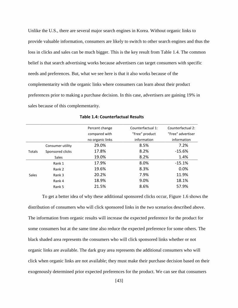
[43]

Unlike the U.S., there are several major search engines in Korea. Without organic links to

provide valuable information, consumers are likely to switch to other search engines and thus the

loss in clicks and sales can be much bigger. This is the key result from Table 1.4. The common

belief is that search advertising works because advertisers can target consumers with specific

needs and preferences. But, what we see here is that it also works because of the

complementarity with the organic links where consumers can learn about their product

preferences prior to making a purchase decision. In this case, advertisers are gaining 19% in

sales because of this complementarity.

Table 1.4: Counterfactual Results

Percent change Counterfactual 1: Counterfactual 2:

compared with "Free" product "Free" advertiser

no organic links information information

Consumer utility 29.0% 8.5% 7.2%

Totals Sponsored clicks 17.8% 8.2% -15.6%

Sales 19.0% 8.2% 1.4%

Rank 1 17.9% 8.0% -15.1%

Rank 2 19.6% 8.3% 0.0%

Sales Rank 3 20.2% 7.9% 11.9%

Rank 4 18.9% 9.0% 18.1%

Rank 5 21.5% 8.6% 57.9%

To get a better idea of why these additional sponsored clicks occur, Figure 1.6 shows the

distribution of consumers who will click sponsored links in the two scenarios described above.

The information from organic results will increase the expected preference for the product for

some consumers but at the same time also reduce the expected preference for some others. The

black shaded area represents the consumers who will click sponsored links whether or not

organic links are available. The dark gray area represents the additional consumers who will

click when organic links are not available; they must make their purchase decision based on their

exogenously determined prior expected preferences for the product. We can see that consumers

[44]

with positive prior preferences for the product will click sponsored links when they cannot learn

about their true preferences. The light gray area represents the additional consumers who will

click sponsored links after having the ability to first click organic links. We now see consumers

with negative prior beliefs about their preferences who have learned that they actually prefer the

product and are now clicking sponsored links. There are consumers who no longer click

sponsored links because they have learned that they do not prefer the product (dark grey area),

but as we can see, the light gray area outweighs the dark gray area, and thus with the ability to

click organic links, more consumers are now clicking sponsored links, and making purchases.

Figure 1.6: Who clicks sponsored links?

Finally, we find that the consumer welfare will increase by 29% with the presence of

organic links. The reason that this percentage increase is larger than clicks or sales increase is

that, with more information on Jeju Island, some consumers who would have visited the island

and later regretted (as their true utility is lower than the outside option) can avoid making the

0.0%

0.5%

1.0%

1.5%

2.0%

2.5%

3.0%

3.5%

4.0%

-20 -15 -10 -5 0 5 10 15 20 25 30 35 40

Den

sity

of

Co

nsu

mer

s

Prior belief about preference for Jeju

BOTH EXOGENOUS Preferences ENDOGENOUS Preferences

[45]

mistake. Clearly the information from organic links provides great value, and this value can be

further enhanced via search engine optimization.

1.6.1 Counterfactuals: Search Engines Providing Information

We have discussed how organic links impact the effectiveness of search advertising. We will

now discuss what the search engines can do to improve their profitability, the consumers’

welfare, and the advertisers’ sales. In these counterfactuals, we compare two potential search

engine policy changes. We assume the search engine may provide information about either the

product or the advertisers’ offerings on the search results page, without the consumer having to

click. Search engines are currently utilizing both strategies. A search of “Jeju Island” at Google,

for example, returns photos of the island, a photo-list of points of interest, and a short summary

about the island along the side of the webpage. Consumers can obtain general information about

the product without having to click into websites from organic links. A search of “Beach resorts

at Jeju Island” at Google, as another example, returns a list of resorts with a photos, a user

ratings, and locations of the resorts. These photos, ratings, and locations provide advertiser-

related information to the consumers. The type of information (product or advertiser) that

delivers more profit to the search engine, sales to the advertisers, and welfare to the consumers

may indicate a prescription for what information the search engine should provide. Note that

while we do not model search engine competition, improving consumer welfare may lead to

increased consumer searches thus brings more revenue to search engines.

In this exercise, we assume the search engine provides "free" information without

incurring search costs for consumers. For the first policy experiment, we assume that the product

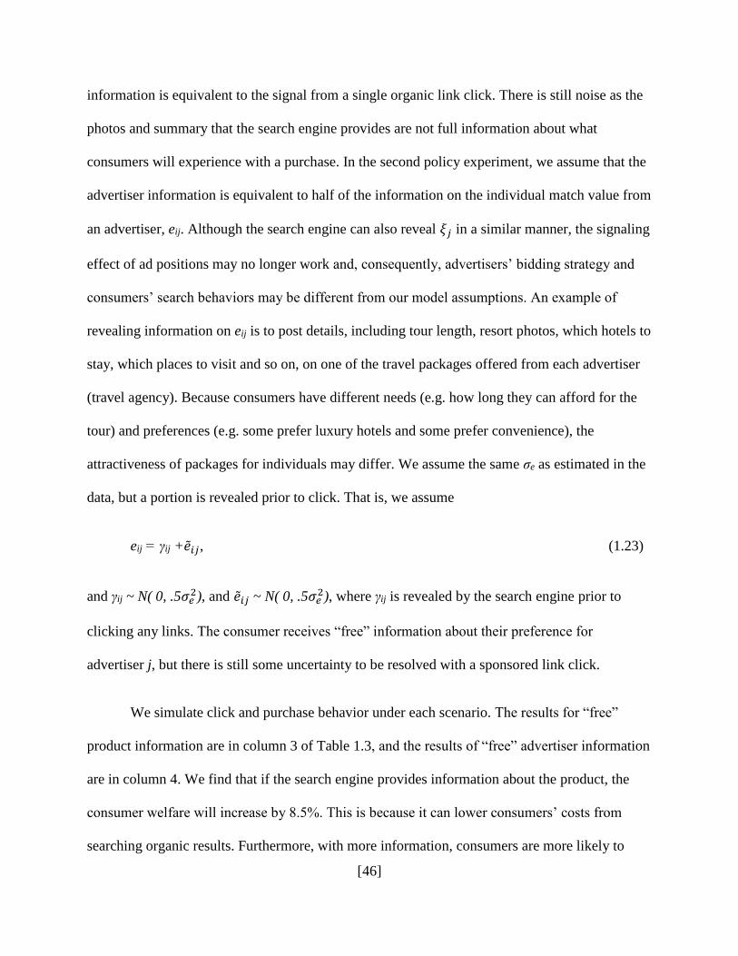
[46]

information is equivalent to the signal from a single organic link click. There is still noise as the

photos and summary that the search engine provides are not full information about what

consumers will experience with a purchase. In the second policy experiment, we assume that the

advertiser information is equivalent to half of the information on the individual match value from

an advertiser, eij. Although the search engine can also reveal 𝜉𝑗 in a similar manner, the signaling

effect of ad positions may no longer work and, consequently, advertisers’ bidding strategy and

consumers’ search behaviors may be different from our model assumptions. An example of

revealing information on eij is to post details, including tour length, resort photos, which hotels to

stay, which places to visit and so on, on one of the travel packages offered from each advertiser

(travel agency). Because consumers have different needs (e.g. how long they can afford for the

tour) and preferences (e.g. some prefer luxury hotels and some prefer convenience), the

attractiveness of packages for individuals may differ. We assume the same σe as estimated in the

data, but a portion is revealed prior to click. That is, we assume

eij = γij +�̃�𝑖𝑗, (1.23)

and γij ~ N( 0, .5𝜎𝑒2), and �̃�𝑖𝑗 ~ N( 0, .5𝜎𝑒

2), where γij is revealed by the search engine prior to

clicking any links. The consumer receives “free” information about their preference for

advertiser j, but there is still some uncertainty to be resolved with a sponsored link click.

We simulate click and purchase behavior under each scenario. The results for “free”

product information are in column 3 of Table 1.3, and the results of “free” advertiser information

are in column 4. We find that if the search engine provides information about the product, the

consumer welfare will increase by 8.5%. This is because it can lower consumers’ costs from

searching organic results. Furthermore, with more information, consumers are more likely to

[47]

avoid regrettable purchase decisions. For the search engine, there is an 8.2% increase in paid

clicks. This is because, for reasons similar to those previously discussed, with more information

on the product, some consumers who would not have clicked on sponsored links learn that they

would prefer the product and these consumers outweigh those who learn that they do not prefer

the product. Consequently, advertisers are also able to generate 8.2% more sales from search

advertising.

When the search engine provides advertiser information instead, it will experience a 15%

drop in paid clicks. This is because there is less uncertainty regarding advertisers’ match value to

resolve, and thus less incentive to click in and resolve such uncertainty. Consumers who would

have been likely to search 4 or 5 advertisers to find their best match are now much more likely to

search 1 or 2 advertisers, be confident that they have found their best match, and stop their

search. Despite receiving fewer clicks, advertisers will generate a 1.4% increase in sales. This

increase is small because consumers are not learning about whether or not they want to purchase

the product, they are learning, if they do wish to purchase, which seller to purchase from. The

top-ranked advertiser, however, has a 15% decrease in sales, while the fifth-ranked advertiser has

a 58% increase in sales. This occurs because, without any advertiser information, consumers who

are indifferent between advertisers will click high-ranked links due to the signaling effect. With

advertiser information, consumers whose revealed preference for the fifth-ranked advertiser, γi5,

is high, may now find it optimal to click that link instead of the top-ranked link. Finally, the

consumer welfare will increase by 7.2% due to reduced search costs and better matching, but this

benefit is smaller than when the search engine provides product information.

The above results only come from partial equilibrium analysis as the impact of the policy

changes on advertisers’ strategy has not been taken into account. Specifically, the free advertiser

[48]

information (the second policy experiment) has two effects on advertiser bidding incentive. First,

the mitigation in rank effect of search ad positions (the top-rank receives 15% fewer sales and

the 5th-rank 58% more sales) may lead to diminished competition among advertisers for these

positions, as there is less incentive to increase bids to obtain higher rankings. Second, in

aggregate, the decrease in paid clicks and the slight increase in sales imply that the conversion

rate will increase, which will increase the value of each ad position. When product information is

provided (the first policy experiment), neither of these effects occurs: the rank effect and the

conversion rates remain relatively constant. To understand the complete impact of these policy

simulations on the search engine and advertisers, we model the optimal advertiser bidding

strategy under both scenarios and quantify the impact on these agents. We use the optimal

bidding strategy in a generalized second price auction, developed in Varian (2007), to study the

change in advertiser bidding following the policy changes. Edelman et al. (2007) show that in a

generalized second price auction, advertisers will not simply bid their willingness-to-pay per

click. They will bid up to their willingness-to-pay and then reduce these bids in order to

maximize profits. Varian derives a range of equilibrium bids, conditional on the mean match

value 𝜉𝑗 and ad position, for each advertiser. We perform two simulations: one assuming firms

bid according to the lower bound, and one assuming firms bid according to the upper bound. The

advertiser’s value per click is calculated as the product of its conversion rate and margins. Both

the conversion rate and margin are estimated as functions of 𝜉𝑗. Given 𝜉𝑗, the advertiser predicts

these values, and then bids according to Varian (2007). We assume the margin to be

proportional16 to the difference in value, averaged across simulated consumers, between the

firm’s offering, 𝐸𝑈𝑖𝑗∗ , and the next best alternative, max {0, 𝑚𝑎𝑥𝑘≠𝑗{𝐸𝑈𝑖𝑘}}, conditional that

16 Advertiser bids are a linear function of this proportion, and thus profit is a linear function of this proportion.

Results, as percent changes in revenue, are unaffected by changes in this proportion.

[49]

𝐸𝑈𝑖𝑗∗ is the consumer’s best option among all sponsored links and the outside option, 𝐸𝑈𝑖𝑗

∗ =

max {0, 𝑚𝑎𝑥𝑘{𝐸𝑈𝑖𝑘}}. This implies that firms with a better offering, a higher 𝜉𝑗, earn a higher

profit per sale. We also assume a 6th advertiser, r, is in the market. This competitor has an

average match value of 𝜉𝑟 drawn from the N(0,1) distribution and truncated above by 𝜉5. Given

𝜉𝑟, advertiser r will bid accordingly. With the generalized second price auction, the advertiser in

the 5th slot will pay according to r’s bid. We also perform this simulation with 5 additional

competitors and obtain similar results.

The simulation results can be found in Table 1.5. We report the changes in average

equilibrium cost-per-click (CPC), determined by advertiser bid amounts, for each ad position as

compared to our original empirical setup (the base model). We also report the changes in

revenue. The results are similar whether advertisers bid according to either the upper or lower

bound. The equilibrium bidding strategy when the search engine provides free product

information is relatively unchanged, as the average winning bid for each ad position is similar to

that of the base model. For the search engine, the 8.2% increase in paid clicks translates to an

8.2% increase in the revenue (see the last two rows in column 3 of Table 1.5). When the search

engine offers free advertiser information, the lower bound and upper bound bid amounts for each

ad position have increased significantly. This is because, in aggregate, the decrease in paid clicks

and the slight increase in advertiser sales (see the last column in Table 1.4) imply an increase in

the conversion rate of each sponsored click. The increase in advertiser bids, however, does not

outweigh the decrease in revenue due to fewer paid clicks, many of which were from the top-

ranked advertiser who is paying the most per click. The net effect is that the search engine’s

revenue decreases by 6% (see the last two rows in the last column of Table 1.5). These results

[50]

are robust to using either upper or lower bounds of advertises’ equilibrium bidding strategy.17

The key results here will reverse if q̅ is positive, rather than negative. This would represent a

product for which the majority of consumers will purchase, if they receive no further information

about the product. Given additional information, some portion of these consumers may learn

about, and then choose, a different preferred option instead. Such a situation is likely to be

uncommon, as the majority of keyword search involves very low click-through and conversion

rates on commercial websites.

Table 1.5: Counterfactual Bidding Results

Percent change from base model

"Free" organic "Free" advertiser

information information

Rank 1 0.0% 11.0%

CPC Rank 2 0.1% 13.8%

Upper Rank 3 0.1% 18.2%

Bound Rank 4 0.2% 18.2%

Rank 5 0.3% 25.2%

Rank 1 -0.1% 11.7%

CPC Rank 2 0.2% 13.8%

Lower Rank 3 0.1% 19.6%

Bound Rank 4 0.2% 20.3%

Rank 5 0.1% 27.0%

Search Engine Upper Bound 8.3% -6.2%

Revenue Lower Bound 8.3% -6.0%

The counterfactual results provide a prescription for search engines on how to utilize

search result page space. If choosing between offering general information about the product or

information about the individual advertisers, we show that product information is likely to

17 To test the robustness of these results to other levels of product and advertiser uncertainty, we recalculate these

results such that the consumers’ uncertainty regarding their match with the product, 𝜎12, and their match with the

advertisers, 𝜎𝑒2, vary from 1/8x to 8x their estimated values. With these manipulations, the results remain highly

robust. Two changes may occur. First, the consumer will gain more welfare from advertiser information, as opposed

to product information, once their uncertainty regarding advertiser fit is sufficiently large. Second, the advertisers

will gain more total sales when advertiser information is provided, as opposed to product information, when the

consumers’ product uncertainty is sufficiently small.

[51]

provide higher consumer welfare, more paid clicks for the search engine, more sales for

advertisers, and increased the revenue from selling keyword ad positions. Search engines,

therefore, should move toward providing more information about the product on the search

results page. It is not clear whether the search engine should discontinue providing advertiser

information because the consumer welfare has increased, which is important for generating more

searches at the search engine.

1.7 Conclusion

The common belief is that search advertising works because advertisers can target consumers

with specific product preferences. We show that for many consumers, sponsored search results

alone are not a sufficient condition for search advertising to work. Organic results, which

primarily lead users to web pages that provide general information on the product, are critical to

induce clicks on sponsored links and convert those clicks into purchases. By allowing consumers

to access content that satisfies their information requirements, informational organic results can

allow consumers to learn about the product category prior to making their purchase decision, and

thus they can make better decisions.

We develop a model characterize the situation in which consumers can search for general

information about the product category as well as for information about the individual sellers’

offerings. We adopt the “ranked search” model to model the sponsored search context in which

consumers can search through a list of options which have been ranked according to average

consumer preferences, in order to find their best match. We estimate this model using a unique

[52]

dataset of search advertising in which commercial websites are restricted in the organic listing.

Organic links are therefore purely for general information, allowing us to identify consumer

clicks as informational (from organic links) or purchase oriented (from sponsored links). With

the estimation results, we show that consumer welfare is improved by 29%, while advertisers

obtain 19% more sales, and search engines receive 18% more paid clicks, as compared to the

scenario without organic links. Furthermore, using counterfactuals we investigate the welfare

changes for consumers, advertisers, and the search engine when the search engine provides

consumers more reliable and precise information about the product or about the advertisers’

offerings in addition to the organic listings. We find that consumers, higher-ranked firms, and the

search engine are likely to be significantly better off when the search engine provides product-

related information rather than advertiser-related information. Based on Varian (2007), we find

that advertiser bids will remain constant when the search engine provides free product

information. When the search engine provides free advertiser information, advertisers will

increase their bids because of the increased conversion rate; however, the search engine still

loses revenue due to the decreased paid clicks. The findings shed important managerial insights

on how to improve the effectiveness of search advertising in terms of attracting clicks and

converting clicks into actions and purchases.

[53]

1.8 References

Agarwal, Ashish, Kartik Hosanagar and Michael D. Smith (2011), “Location, Location,

Location: An Analysis of Profitability of Position in Online Advertising Markets,” Journal of

Marketing Research, 48 (6), 1057-1073.

Aggarwal, Gaurav, Jon Feldman, and S. Muthukrishnan (2006), “Bidding to the Top: VCG and

Equilibria of Position-Based Auctions,” Approximation and Online Algorithms. Lecture

Notes in Computer Science. Springer, Berlin, 15-28.

Athey, Susan and Glenn Ellison (2011), “Position Auctions with Consumer Search,” Quarterly

Journal of Economics, 126 (3), 1213-1270.

Bentley, Taylor, Tat Y. Chan and Young-Hoon Park (2014), “Testing the Signaling Theory

Using Data in Search Advertisements,” Working Paper, Washington University, St. Louis.

Chan, Tat Y., Chunhua Wu, and Ying Xie (2011), “Measuring the Value of Customer

Acquisition from Search Advertising,” Marketing Science, 30 (5)

Chan, Tat Y. and Young-Hoon Park (2014), “The Value of Consumer Search Activities for

Sponsored Search Advertisers,” Working Paper, Washington University, St. Louis.

Chen, Yongmin and Chuan He (2011), “Paid Placement: Advertising and Search on the

Internet,” Economic Journal, 121 (56), F309-F328.

De Los Santos, Babur, Ali Hortacsu, and Matthijs R. Wildenbeest (2012), “Testing Models of

Consumer Search Using Data on Web Browsing and Purchasing Behavior,” American

Economic Review, 102 (6), 2955-2980.

[54]

Edelman, Benjamin and Michael Ostrovsky (2007), “Strategic Bidder Behavior in Sponsored

Search Auctions,” Decision Support Systems, 43 (1), 192-198.

Edelman, Benjamin, Michael Ostrovsky and Michael Schwarz (2007), “Internet Advertising and

the Generalized Second Price Auction: Selling Billions of Dollars Worth of Keywords,”

American Economic Review, 97 (1), 242-259.

Ghose, Anindya and Sha Yang (2009), “An Empirical Analysis of Search Engine Advertising:

Sponsored Search in Electronic Markets,” Management Science, 55 (10), 1605-1622.

Goldfarb, Avi and Catherine Tucker (2011), “Search Engine Advertising: Channel Substitution

When Pricing Ads to Context,” Management Science, 57 (3), 458-470.

Honka, Elisabeth and Pradeep Chintagunta (2014), “Simultaneous or Sequential? Search

Strategies in the U.S. Auto Insurance Industry,” Working Paper, University of Texas, Dallas.

Hortaçsu, Ali and Chad Syverson (2004), "Product Differentiation, Search Costs, and

Competition in the Mutual Fund Industry: A Case Study of S&P 500 Index Funds," Quarterly

Journal of Economics, 119(2), pp. 403.

Jerath, Kinshuk, Liye Ma, and Young-Hoon Park (2014), “Consumer Click Behavior at a Web

Search Engine: The Role of Keyword Popularity,” Journal of Marketing Research,

forthcoming.

Erdem, Tülin and Michael P. Keane (1996), “Decision-Making under Uncertainty: Capturing

Dynamic Brand Choice Processes in Turbulent Consumer Goods Markets,” Marketing

Science, 15 (1), 1-20.

[55]

McCall, J. J. (1970), “The Economics of Information and Job Search,” Quarterly Journal of

Economics, 84 (1), 113-126.

McFadden, Daniel (1989) "A method of simulated moments for estimation of discrete response

models without numerical integration," Econometrica, 57, 995-1026.

Milgrom, Paul R. and Robert J. Weber (1982), “A Theory of Auctions and Competitive

Bidding,” Econometrica, 50 (5), 1089-1122.

Mortensen, Dale T. (1970), “Job Search, the Duration of Employment and the Phillips Curve,”

American Economic Review, 60, 505-517.

Narayanan, Sridhar and Kirthi Kalyanam (2014), “Position Effects in Search Advertising: A

Regression Discontinuity Approach,” Working Paper, Stanford University.

Rutz, Oliver and Randolph E. Bucklin (2011), “From Generic to Branded: A Model of Spillover

in Paid Search Advertising,” Journal of Marketing Research, 48 (1), 87-102.

Stigler, George J. (1961), “The Economics of Information,” Journal of Political Economy, 69

(3), 213-225.

Varian, Hal R. (2007), “Position Auctions,” International Journal of Industrial Organization, 25

(6), 1163-1178.

Vickrey, William (1961), “Counterspeculation, Auctions, and Competitive Sealed Tenders,” The

Journal of Finance, 16 (1), 8-37.

Weitzman, Martin L. (1979), “Optimal Search for the Best Alternative,” Econometrica, 47 (3),

641-654.

[56]

Yang, Sha and Anindya Ghose (2010), “Analyzing the Relationship Between Organic and

Sponsored Search Advertising: Positive, Negative, or Zero Interdependence?,” Marketing

Science, 29 (4), 602-623.

Yao, Song and Carl F. Mela (2011), “A Dynamic Model of Sponsored Search Advertising,”

Marketing Science, 30 (3), 447-468.

[57]

Chapter 2:

Testing the Signaling Theory of Advertising:

Evidence from Search Advertisements

2.1 Introduction

Since Nelson (1970, 1974), a stream of theoretical works (e.g., Klein and Leffler 1981,

Grossman and Shapiro 1984, Milgrom and Roberts 1986, Bagwell and Riordan 1991, Meurer

and Stahl 1994, Anderson and Renault 2006) have been developed to formalize the signaling

theory of advertising. However, empirical evidence supporting the signaling function of

advertising is rather limited. In this paper, we empirically test the theory using a rich micro-level

dataset of search advertising obtained from a search engine. Although alternative explanations

for why advertising helps increase sales, including the persuasive and informative functions of

advertising, are available in the literature, the signaling theory provides unique insights into how

both consumers and advertisers strategically behave in markets with differentiated products. In

such markets, consumers have uncertainty regarding the attributes of product offerings, and it is

costly for them to search for product information. The theory predicts that, under general

conditions, firms with products that can better match with consumer needs and preferences will

spend more on advertising to signal the high “match value” of their products. This is because

advertisers expect that consumers, after being exposed to the advertising signal, will infer that

their products are more likely to meet their needs. At equilibrium, consumers make such rational

inferences based on the signals, leading to the positive correlation between advertisement

[58]

spending and sales or consumer quality perception. Since the theory has major implications for

firm competition and welfare analysis, testing the validity of the theory with real market data is

important to firms, policy makers, and academic researchers.

We choose the search advertising market for this study for several reasons. First, search

advertising has played a dominant role in the advertising industry. According to a report from the

Interactive Advertising Bureau (http://www.iab.net/AdRevenueReport), internet advertising

revenues have soared to $42.8 billion in the U.S. in 2013, surpassing broadcast television

advertising revenues for the first time. Search advertising is the leading internet advertising

format. It has a 43% share of internet advertising revenues, reaching $18 billion, much higher

than all other formats including display advertising ($13 billion) and mobile advertising ($7

billion). Understanding the underlying mechanisms that drive the effectiveness of search

advertising thus is substantively important. Second, the nature of search advertising offers an

ideal environment for testing the signaling theory. In many cases, using keyword search implies

that consumers have uncertainty for keyword-related products or services, a necessary condition

for signaling theory to work. Another key condition is that consumers have knowledge on which

firms spend more on advertising. Since consumers observe the ad positions of sponsored links on

the search results page, it is reasonable to assume that they can infer advertisers at higher

positions pay more for their clicks, via keyword auctions, than advertisers at lower positions. In

contrast, this condition may not be satisfied in other markets such as print and TV advertising.

Finally, although past research has tested the relationship between demand and advertising

spending and, in the case of search advertising, the impact of ad positions on consumer clicks

and purchases, there are no empirical studies testing whether firm strategies are consistent with

the predictions from the signaling theory. The rich micro-level data that we use in the study

http://www.iab.net/AdRevenueReport

[59]

enables us to test the theory not only on consumer but also on firm behaviors. Alternative

explanations for why advertising works have to be examined. As we will discuss in the section of

literature review, testing firm behaviors and ruling out alternative explanations are a challenging

task in previous empirical studies because they use aggregate data sourced from a single

advertising firm which lack data on other advertisers.

In this study, we choose several travel-related keywords that have different properties

associated with consumer needs and preferences. The data provides detailed information on both

consumers and advertisers, including the identity of every advertiser whose sponsored link is

visible to consumers, their ad positions on the search results page, and the entire sequence of

clicks for every keyword search made by consumers. We also observe for each advertiser how

much it pays as well as how much it bids for a click on its sponsored link. Therefore, we are able

to test not only the demand side but also the supply side behaviors predicted by the theory. A

typical advertiser (e.g., travel agency) in data carries a full line of differentiated travel services

(e.g., packaged tours, flights, hotels, car rentals). For many service attributes, it is impossible for

consumers to know all details by just browsing the search results page. Searching for the details

at each advertiser’s website, however, is very time-consuming. Consumers therefore may rely on

the signals they observe from search advertisements to determine their clicking and purchasing

decisions.

We test three main hypotheses that are developed from the signaling theory of

advertising. Our empirical tests show that, on the consumer side, sponsored links at high ad

positions attract more clicks even after controlling for advertiser fixed effects. Furthermore,

consumers are more likely to choose high-positioned sponsored links for terminal clicks, the last

link clicked in the search process. We argue that terminal clicks and the probability that

[60]

consumers find a match should be positively correlated. This result therefore is consistent with

the prediction that the offerings from advertisers at higher (lower) positions match with the needs

and preferences for a larger (smaller) proportion of consumers. We also test the advertiser

behaviors as predicted by the theory using a unique feature in the data. Advertisers frequently

adjust their bids for a click within a day but, because of the uncertainty regarding how much their

competitors will bid, it is possible that their ad positions remain unchanged. Empirical tests using

these observations show that an advertiser’s decision to increase its bids is positively correlated

with terminal clicks. Yet, without changing ad positions, there is no significant correlation

between bid amounts and clicks. This provides significant evidence that advertisers’ bid

decisions are based on the match value that has to be signaled, and not solely the information that

consumers already know prior to clicking sponsored links.

We further examine whether alternative explanations for how advertising works can

account for these results. Making use of the individual-level consumer search data, we test how

consumer clicks are correlated with changes in ad positions within a day and find similar results,

implying that our findings are unlikely to be driven by external factors (e.g., advertising

campaigns in other media) that may increase the click potential which we as researchers do not

observe. We also show that the persuasive and informative functions of advertising, as well as

the consumer non-strategic top-down search behavior, cannot fully explain our findings. In sum,

these results provide thorough support that signaling is at work in our empirical context. Finally,

we further illustrate from data an important phenomenon of informational externality, where a

sponsored link with higher match value has a positive spillover effect on other sponsored links

listed above or below. The signaling theory offers an explanation for this finding.

[61]

2.1.1 Related Literature

Nelson (1970, 1974) argues that firms in an experience goods market have incentive to advertise

heavily to signal the quality of their products. Later works (e.g., Grossman and Shapiro 1984,

Milgrom and Roberts 1986, Meurer and Stahl 1994, Anderson and Renault 2006) formalize the

idea by developing a game-theoretic model in which high-quality firms are incentivized to spend

more on advertising to signal but low-quality firms do not find it profitable to mimic. Klein and

Leffler (1981) endogenize product quality in the signaling model. Bagwell and Riordan (1991)

develop a model for durable goods, where price instead of advertising is used to signal product

quality, and show that at equilibrium high-quality firms will charge more than the full

information price.

A stream of empirical research follows the theoretical development by using aggregate

data to test how the signaling theory applies to advertising. Tellis and Fornell (1988), for

example, use PIMS datasets to examine how product quality (represented by the difference

between the percentage of sales of products superior to competing products and the percentage of

sales inferior) is affected by advertising. Caves and Greene (1996) use Consumer Reports to

examine the relationship between quality ratings and advertising outlays of product brands.

Thomas et al. (1998) use data from the U.S. automobile industry and find a positive association

between future sales and current advertising levels. The challenge with using aggregate data is

that it is difficult to rule out alternative explanations. This is because the relationship between

advertising and sales or quality rankings can be due to other unobserved factors (e.g., changed

product quality) or other functions of advertising unrelated to quality signaling. Because of this

issue, another stream of research uses experimental data to investigate how participants’

[62]

perceived product quality changes under manipulated conditions of advertising spending (e.g.,

Kirmani and Wright 1989, Kirmani 1990, Moorthy and Hawkins 2005).

Our research differs from the existing studies in a few important ways. Our study uses

rich micro-level data that help test the theory against other alternative explanations, instead of

aggregate-level data. It also differs from the experimental literature by using observational data

which is important for the external validity of the study. Most importantly, because we obtain

data on not only how consumers search but also how advertisers bid, we are able to study the

strategic behaviors on the firm side, which has never been tested in the previous literature,

simultaneously with the consumer behavior predicted by the theory.

In the search advertising context, a number of empirical studies have documented the

effects of ad positions on clicks and purchase conversions (e.g., Ghose and Yang 2009, Yang and

Ghose 2010, Agarwal et al. 2011, Goldfarb and Tucker 2011, Rutz and Bucklin 2011, Yao and

Mela 2011, Chan and Park 2014). The common result is that the number of clicks increases as

advertiser position moves up in the sponsored list. Recently, Narayanan and Kalyanam (2014)

find a few moderators of the positions effects, and show that the effects are weaker for smaller

firms and for keywords with less prior consumer experience. These empirical findings have

served as the basis for a large stream of research in search adverting (and also served as a

guideline for practitioners), but limited research is available to examine the underlying

mechanisms of the position effects in search advertising. The exceptions are the theoretical

works of Athey and Ellison (2011) and Chen and He (2011), who apply the signaling theory to

explain the positive position effects. They study the optimal bidding strategy of advertisers with

heterogeneous products or services competing against each other for search ad positions. Their

analyses show that, for consumers with heterogeneous needs and preferences who are searching

[63]

for product information, when they can rationally infer the equilibrium auction outcomes,

advertisers with high match value (i.e., their product offering can match with the needs and

preferences of a large proportion of consumers) will bid more for high ad positions, since more

relevant advertisers will benefit more from attracting consumers to their website. We therefore

observe a separating equilibrium.18 The signaling approach we use in this study is based on their

models.19

To the best of our knowledge, this is the first paper that provides empirical evidence that

firms use ad positions in search advertising to signal advertiser match value, which will influence

consumers’ search behaviors. As the signaling theory has major implications for firm

competition and welfare analysis, our findings are important to firms, policy makers, and

academic researchers.

18 Jerath et al. (2011), however, show that it may also be optimal for a low-quality advertiser to outbid high-quality

competitors. This “Position Paradox” occurs when some portion of the consumers are knowledgeable about the

firms’ offerings and high-quality advertisers drop their bids to save cost, they do not lose too many clicks to inferior

advertisers. It may be optimal for low-quality advertisers to maintain a high bid to attract potential consumers before

they browse and click links from high-quality advertisers. 19 Search advertising has attracted much research interest in the economics and marketing literature. On the firm

side, researchers have focused on the bidding strategies and advertiser competition in position auctions for

keywords. In generalized second price auctions, equilibrium bidding strategies of which bidders bid optimally by

their value per click have been studied (e.g., Edelman et al. 2007, Varian 2007). Chan and Park (2014) model the

decisions of advertisers and propose using the method of moment inequalities when optimal conditions are not well

defined. Yao and Mela (2011) structurally model advertisers’ dynamic bidding decisions assuming asymmetric

valuations of sponsored positions for advertisers. Edelman and Ostrovsky (2007) estimate advertiser valuations

without uncertainty in the search environment, and Athey and Nekipelov (2012) develop a homotopy-based method

for computing equilibria when there is uncertainty about the set of competitors and individual users, and competing

bids. Our research is also closely related to how consumers search for product information in the optimal sequence.

Past literature has studied either non-sequential search (e.g., Stigler 1961) or sequential search (e.g., McCall 1970,

Weitzman 1979). Kim et al. (2009) apply the Weitzman framework to model the optimal dynamic search process of

consumers when shopping for camcorders at Amazon.com. De los Santos et al. (2012) use data on browsing and

prices across websites to test different search models and argue that non-sequential search is more consistent with

the data than sequential search and that consumers may update their belief of the distribution of prices during the

search. Honka and Chintagunta (2014) use data on consumer shopping behavior in the U.S. auto insurance industry

to identify the search strategy consumers use and argue that the largest insurance companies are better off when

consumers search sequentially, while smaller companies profit from consumers searching simultaneously.

[64]

The remainder of the paper is organized as follows. Section 2 discusses the data. We

outline the signaling model and present the key hypotheses to be tested in section 3. Section 4

presents the results of the hypotheses testing. In section 5, we test against several alternative

explanations and conclude that our findings cannot be fully explained by these explanations.

Section 6 explores an extended test of the data. We conclude with directions for future research

in section 7.

2.2 Data

The data are from a leading search engine firm in Korea. In response to a keyword search, a list

of sponsored ads is placed at the top of the search results page, with a maximum of five ads

displayed. The search engine decides which sponsored links are displayed in which order, based

on a second-price position auction similar to what Google uses; however, no quality score based

on a link’s click potential is applied. Each advertiser pays each time the link is clicked, this is

known as the cost-per-click (CPC) pricing. A list of organic links is placed below the list of

sponsored links.20 Our data provider noted that commercial websites, which sell products related

to search queries, are restricted from the organic listing. As such, there is negligible overlap

between the links displayed in the organic (informational) and sponsored (commercial) listings.

To be viewed by the consumer during the search, advertisers must bid to be placed in the

sponsored listing. Organic links are chosen from a proprietary database consisting of different

types of related content, such as general information pages on the topic (e.g., pages from

20 We note that this layout is similar to the layout of popular US search engines such as Google and Bing, which

display several (typically, up to three) sponsored links on the top of the results page following by the organic link.

We refer readers to Jerath, Ma, and Park (2014) for details of the data.

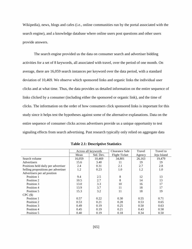
[65]

Wikipedia), news, blogs and cafes (i.e., online communities run by the portal associated with the

search engine), and a knowledge database where online users post questions and other users

provide answers.

The search engine provided us the data on consumer search and advertiser bidding

activities for a set of 8 keywords, all associated with travel, over the period of one month. On

average, there are 16,059 search instances per keyword over the data period, with a standard

deviation of 10,469. We observe which sponsored links and organic links the individual user

clicks and at what time. Thus, the data provides us detailed information on the entire sequence of

links clicked by a consumer (including either the sponsored or organic link), and the time of

clicks. The information on the order of how consumers click sponsored links is important for this

study since it helps test the hypotheses against some of the alternative explanations. Data on the

entire sequence of consumer clicks across advertisers provide us a unique opportunity to test

signaling effects from search advertising. Past research typically only relied on aggregate data

Table 2.1: Descriptive Statistics

Across all keywords Clearance Sale Travel Travel to

Mean Std. Dev. Flight Ticket Agency Jeju Island

Search volume 16,059 10,469 34,801 26,163 19,479

Advertisers 15.6 3.40 11 19 19

Positions held daily per advertiser 2.4 0.31 2.1 2.7 2.8

Selling propositions per advertiser 1.2 0.23 1.0 1.2 1.0

Advertisers per ad position

Position 1 9.4 2.5 8 12 13

Position 2 10.5 2.7 8 14 13

Position 3 13.0 3.3 10 16 17

Position 4 13.9 3.7 11 18 17

Position 5 15.3 3.2 11 18 19

CPC ($)

Position 1 0.57 0.22 0.30 0.55 0.71

Position 2 0.53 0.21 0.28 0.53 0.65

Position 3 0.49 0.19 0.25 0.50 0.63

Position 4 0.45 0.19 0.21 0.43 0.58

Position 5 0.40 0.19 0.18 0.34 0.50

[66]

sourced from a single advertiser. Based on the sequence of clicks made by an individual

consumer, we can correctly identify which link is the last one that a consumer clicks during the

search process; thus, unlike Chan and Park (2014) we do not rely on behavioral assumptions

(e.g., top-down browsing and sequential search) to infer terminal clicks.

We also observe from the data the identity of each advertiser displayed in the sponsored

listing in response to a consumer’s search query. On average, as shown in Table 2.1, there are

15.6 advertisers per keyword competing for ad positions in the sponsored section. This is

different from previous works (e.g., Ghose and Yang 2009, Yang and Ghose 2010, Agarwal et

al. 2011, Rutz and Bucklin 2011) which often lack data on the complete list of sponsored links

presented to consumers, as their data source comes from a single advertiser. In addition, we have

data on advertisers’ bid amounts and the prices they pay. An advertiser’s position may change

throughout the day as it alters its bid. There is significant variation in ad positions obtained by

advertisers within a single day in data. The third row in Table 2.1 shows that the average number

of ad positions per advertiser per keyword is 2.4 per day, with a standard deviation of 1.2. The

table also presents the descriptive statistics for the top three most searched keywords, “Clearance

Sale Flight Ticket”, “Travel Agency”, and “Travel to Jeju Island”, all demonstrating similar

patterns. The information on the advertiser bidding activity in sponsored search advertising is

unique since it helps understand how advertisers indeed behave in sponsored search advertising.

We will explain in later sections how we use this daily variation in ad positions to test the effect

of ad positions on click behavior. We also observe advertisers’ selling propositions which

typically highlight current promotions, special travel packages, a website’s unique attributes, and

so on. Most advertisers use the same proposition throughout the data period. The average number

of unique selling propositions for each specific advertiser-keyword combination is 1.2. Table 2.1

[67]

shows that selling propositions have never been changed for “Clearance Sale Flight Ticket” and

“Travel to Jeju Island” during the data period. The table also provides the information on the

average number of advertisers who obtains each position. On average, 9.4 advertisers are placed

at the topmost position at some point in the data period, while 15.3 advertisers obtain the fifth

position. This indicates significant changes in advertisers’ bidding activity for these keywords in

the data period.

It is worth discussing that the travel-related category satisfies several criteria for

empirically testing the signaling theory in the search advertising context. First, consumers

typically have large uncertainty regarding the travel services that they search. Searches can be

costly as it takes time to browse and process all details provided from travel websites. Second, on

the advertiser side, the travel service market is highly fragmented, with many competing service

providers without anyone dominating. Consumers are not likely to have full information on the

service offerings from every website prior to clicking its sponsored link. Advertisers’ offerings,

and thus their match values, change frequently as airline seats sell out, hotels fill up, they receive

blocks of tickets on promotion, and flight dates approach.

In addition, the travel-related category has a few important data features which help

statistical testing. First, we observe a large number of search instances and active bidding from

advertisers to obtain ad positions, with all five ad positions being occupied for the majority of the

search instances (97.2%). As such, we avoid small sample issues for statistical testing. Second,

each ad position has been occupied by many different advertisers (see Table 2.1). This helps us

to separate the advertiser fixed effects from the effects of ad positions. For each advertiser, ad

positions also vary across search instances, implying intensive competition among the

advertisers. Third, we observe significant variations in CPC across ad positions, ranging from an

[68]

average of $0.57 for the topmost position to an average of $0.40 for the fifth position (see Table

2.1).21 We also observe significant variation in CPC for the same position and the same keyword

during the data period. Fourth, for the purpose of testing alternative explanations for our

findings, it would be desirable to have keywords that are narrowly defined (e.g., “Flight Ticket to

Jeju Island”) and some keywords that are more general (e.g., “Flight Ticket”), and keywords

focusing on a specific attribute (e.g., price in “Clearance Sale Flight Ticket”) and some which are

more comprehensive (e.g., “Flight Ticket”). The purpose for this criterion will become clear later

in the paper. Furthermore, because our research objectives are related to firm sales, we look for

keywords that are relatively more likely to indicate the purchase intention from consumers. For

example, a keyword search for “Flight Ticket to Jeju Island” is likely to be related to the

intention of buying tickets, while a keyword search for “Jeju Island” may only serve for

informational purposes.

2.3 The Signaling Model and Hypotheses

This section outlines the signaling model and describes how it is applied to the search advertising

context. We highlight a set of testable predictions on the behaviors of consumers and advertisers,

which constitute the signaling theory. Since our modeling approach is similar to Athey and

Ellison (2011) and Chen and He (2011), we refer readers who are interested in how the

equilibrium outcomes are derived to their papers for details.

We consider each search instance in the data as a search query made by an individual

consumer. Athey and Ellison (2011) assume that each advertiser differs in the match value, i.e.,

21 We note that all bids are in Korean currency (won), where 1000 won corresponds approximately to $1.

[69]

the probability of meeting a consumer’s needs, of its product or service offering, implying that

advertisers are horizontally differentiated. By focusing on horizontal, rather than vertical,

differentiation, we study the most basic case in search advertising, in which search queries could

be sufficiently broad that users may have many different intentions when searching the same

keyword. In such context, the key differentiation among advertisers is the likelihood that their

offerings fit with heterogeneous consumer needs.

Subsequent to a keyword search, consumer i observes advertiser j in the sponsored

listing. To test the signaling theory from data, we use an empirical specification to measure the

likelihood that the advertiser’s offering matches with the consumer’s needs. We assume that the

likelihood is driven by a latent utility that is determined by the advertiser’s offering for

consumer, which is specified as follows:

𝑉𝑖𝑗 = 𝑢𝑖𝑗 + 𝜐𝑖𝑗 . (2.1)

The first component 𝑢𝑖𝑗 is the portion of the utility which the consumer already has information

about prior to clicking the advertiser’s sponsored link. In empirical testing, it is specified as

𝑢𝑖𝑗 = 𝛼𝑗 + 𝑒𝑖𝑗, (2.2)

where 𝛼𝑗 is the value averaged across consumers, and 𝑒𝑖𝑗 is assumed to be iid across consumers.

By definition the average value of 𝑒𝑖𝑗 across consumers is zero. The second component, 𝜐𝑖𝑗, is

the unknown portion of the utility which the consumer can obtain from the advertiser’s website

[70]

by clicking its sponsored link.22 If Vij is larger than a threshold value (normalized to zero in

empirical testing), the match is one, i.e., the consumer finds a match.

As an illustration, suppose the consumer is planning a vacation to Jeju Island, a popular

vacation destination in Korea. She searches the keyword “Flight Ticket to Jeju Island” and finds

a list of sponsored advertisers, including travel agents and airline carriers. The selling

propositions in the ad, which typically consist of a phrase (such as “We offer flights to Jeju

Island from major cities”), may convey information on what the advertiser offers to the

consumer. This information, and the consumer’s prior knowledge about the advertiser, gives the

consumer 𝑢𝑖𝑗. Still, the consumer may have specific needs or preferences regarding the departure

place, date and time of travel, etc. Detailed information of the advertiser’s offerings, captured by

𝜐𝑖𝑗, is not available on the search results page. To find out what flights are available, she has to

search for details from the advertiser’s website. The higher the value of 𝜐𝑖𝑗, the higher the

likelihood that the consumer finds the advertiser’s offering a good match. In empirical testing,

we use a reduced-form way to specify this component as follows:

𝜐𝑖𝑗 = 𝜉𝑗 + 휀𝑖𝑗 , (2.3)

where 𝜉𝑗 represents the average match value across consumers, and 휀𝑖𝑗 captures the individual-

specific stochastic component whose value is zero averaged across consumers. In the above

example, 𝜉𝑗 will be higher if the advertiser has more flights to Jeju Island from different cities, or

charges lower prices on average. The advertiser can thus match the needs and preferences of

22 For experience goods, consumers still have uncertainty regarding the actual consumption experience which

information is not revealed from the advertiser’s website. We assume that the consumer’s objective is to maximize

the expected value Vij conditional on all of the available information. As long as the uncertainty of post-purchase

experience is independent from the conditional expectation, it will have no impact on the consumer’s search and

purchase decisions.

[71]

more consumers. Some consumers, however, may have low 휀𝑖𝑗 because the advertiser does not

offer a direct flight from their cities to Jeju Island or, even if there is a flight, the price of that

specific flight is higher than the others. Both 𝜉𝑗 and 휀𝑖𝑗 are unknown to consumers by only

seeing selling propositions. We also assume that 휀𝑖𝑗 is iid across advertisers and consumers.

Search advertising is costly for advertisers via second-price auctions. The higher the ad

position the higher the cost an advertiser has to pay for each click. Based on the signaling theory,

consumers use the observed ad positions to infer the unobserved match value of advertisers’

offerings. Therefore, the expected utility of the consumer, prior to clicking the sponsored link,

can be expressed as:

E(𝑉𝑖𝑗|𝑝𝑗) = 𝛼𝑗 + E(𝜉𝑗|𝑝𝑗) + 𝑒𝑖𝑗. (2.4)

Observing that the ad position of advertiser j (𝑝𝑗) is higher than that of advertiser k (𝑝𝑘),

the consumer will rationally infer that E(𝜉𝑗|𝑝𝑗) > 𝐸(𝜉𝑘|𝑝𝑘). At a cost of clicking, 𝑐𝑖, the

consumer can click on the advertiser’s sponsored link. In the above example, the cost comes

from the time of searching for several flights from the departure city to Jeju Island that the

advertiser offers on a specific date, checking for the price information, and possibly searching for

packages with hotels and car rentals. Psychological costs (e.g., processing the information on

flights and their prices) may also incur. Suppose the consumer searches optimally in a sequential

way, she will click on the link if its expected match value, conditional on the ad position of the

link, is higher than other sponsored links that have not been clicked, and the expected benefit of

[72]

clicking the link outweighs the cost of clicking.23 This explains why consumers are more likely

to click on top ad positions, offering us the first hypothesis to be tested:

Hypothesis 1: Top ad positions generate more clicks, after controlling for the partial

information (𝑢𝑖𝑗) that consumers may have prior to clicking.

After the consumer clicks into the advertiser’s website, the match value component 𝜐𝑖𝑗 =

𝜉𝑗 + 휀𝑖𝑗 will be revealed. If the consumer finds the advertiser’s offering a match (i.e., Vij is larger

than the threshold value), she will terminate the search. Otherwise, the consumer will click on

the next link which, among all other links that have not been clicked, has the highest expected

match value, as long as the expected benefit of clicking the link outweighs the cost of clicking.

The process will continue in a similar fashion. When the market is at equilibrium, the

consumer’s belief is consistent with the advertiser’s bidding strategy. That is, if 𝑝𝑗 is higher than

𝑝𝑘 (and thus E(𝜉𝑗|𝑝𝑗) > 𝐸(𝜉𝑘|𝑝𝑘)), 𝜉𝑗 is higher than 𝜉𝑘. Therefore, compared with those who

click at low ad positions, more consumers who click at top ad positions will be able to find a

match.

We do not directly observe the match since we do not have consumer purchase data;

however, we observe the entire sequence of sponsored and organic links that a consumer clicks.

Since consumers will terminate their search after finding a match, we use terminal clicks of

keyword searches to test the prediction. A terminal click refers to the last sponsored or organic

link clicked by a consumer during the search process. We argue that terminal clicks and the

probability that consumers find a match are positively correlated. This assumption is supported

23 In the stylized models in Athey and Ellison (2011) and Chen and He (2011), the link will be the topmost one in

the sponsored listing. In our setup, however, consumer i may start clicking advertiser j listed at a lower position if

the prior knowledge 𝑢𝑖𝑗 is sufficiently high.

[73]

by Chan and Park (2014) who find that, for search advertising, advertisers’ value comes nearly

entirely from such terminal clicks. This result may imply a strong correlation between terminal

clicks and purchase occasions, but the opposite for non-terminal clicks and purchase occasions.

They argue that, since there is little reason why the probability of non-match occasions for

terminal clicks may differ across ad positions, terminal clicks can be a good proxy for the match

likelihood.24 On this logic, non-terminal clicks and terminal clicks on organic links likely

indicate that consumers, after clicking sponsored links, do not find a match from advertisers’

offerings.25 Based on this reasoning, we propose the second hypothesis that focuses on

consumer terminal clicks by ad positions:

Hypothesis 2: Conditional on being clicked, top ad positions have a higher likelihood for

being a terminal click.

Our empirical tests extend beyond the consumer behavior on the search results page. The

signaling theory states that, with a higher match value (𝜉𝑗), an advertiser is willing to bid more

for a high ad position to signal the match value. This is because, after clicking the sponsored

link, a large proportion of consumers will find the offering a good match; thus, each consumer

click is more valuable to the advertiser (see Athey and Ellison 2011). For the theory to work, it is

24 If there is a difference between terminal clicks and the probability of a match across ad positions, it is likely that

lower positions will have a disproportionately lower probability of a match, given a terminal click, for two reasons.

First, a consumer terminating search on a lower link may have searched through higher positioned advertisers and

concluded their search having not found a match. Second, if a consumer were to click multiple links, keeping a tab

with a clicked link open, and then return that link to purchase (we will not observe this in the data), it is relatively

more likely that the observed terminal click will be a lower positioned advertiser and the match was with one in a

higher position. These two points indicate that our results would serve to be conservative due to our use of terminal

clicks. 25 Existing studies use aggregate data sourced from a single advertising firm which includes purchase conversions at

the advertiser. However, they are conducted from the perspective of one single advertiser, and thus lack data on

clicks on sponsored and organic links of other entities on the search results page. In other words, they do not have

sufficient data to give a comprehensive picture of user behavior on the search results page. In this study, we use data

from a search engine and have information on clicks on the full lists of sponsored and organic links presented after a

keyword search.

[74]

important that the bidding decision is driven by 𝜉𝑗, and not entirely by 𝛼𝑗, the part that

consumers already know before clicking the sponsored link. Testing this prediction is difficult,

since consumers’ information set is unobserved to researchers. In this study, we make use of the

panel structure of the data: we observe how bid amounts vary not only across advertisers, but

also over time within advertisers. For each advertiser, 𝜉𝑗 is not necessarily fixed over time.

Available flight times to Jeju Island, for example, may fluctuate within the advertiser, depending

on how many tickets are sold as the flight date gets closer. We observe a unique feature in the

data: often an advertiser’s ad position remains unchanged even when it increases the bid (i.e. the

advertiser cannot outbid any of its competitors at higher positions). This is because the advertiser

has uncertainty regarding how much other advertisers will bid, so the ad position only fluctuates

with bid amounts in a probabilistic way. If the bid decision is driven by the increase in 𝜉𝑗, we

should observe an increase in the likelihood of terminal clicks. However, since 𝜉𝑗 is not observed

by consumers before clicking, the likelihood of clicking the advertiser’s sponsored link should

not increase without the change in ad position. On the other hand, if the bid decision is entirely

driven by the change in 𝛼𝑗, the likelihood of clicking should also change accordingly. Based on

this reasoning, we test the last hypothesis as the following:

Hypothesis 3: The likelihood that an advertiser’s link is chosen for a terminal click

improves (diminishes), as the advertiser bids more (less) even though the ad position

remains unchanged. The likelihood that the link is chosen for a click, however, will not

change.

The three hypotheses constitute the signaling story: Consumers believe higher positioned

advertisers to be of higher match value, advertisers with higher match value are on average in

[75]

higher positions, and when its match value improves, an advertiser increases its bid. This paper

uses rich micro-level data to test these hypotheses. It is important to note that we do not argue

that signaling is the only explanation for observed consumer and advertiser behaviors. A number

of alternative explanations might predict similar outcomes. In a later section, we control for these

non-signaling explanations for the results to investigate whether the signaling effects on both

consumers and advertisers are still present.

2.4 Empirical Analysis and Results

2.4.1 Testing Hypothesis 1

Table 2.2 presents summary statistics about the click-through rate (CTR) and terminal click-

through rate (TCTR) by ad positions. It shows that higher CTR associates with higher ad

positions. This is consistent with the main finding from the empirical work in search advertising

that advertisements at higher positions attract more clicks from consumers (e.g., Agarwal et al.

2009, Feng et al. 2007, Ghose and Yang 2009, Chan and Park 2014). The topmost position is

Table 2.2: Click-Through Rates and Terminal-Click Through Rates



CTR (%)

Position 1 5.1 1.9 6.2 3.3 7.7

Position 2 2.7 1.2 2.9 1.7 5.3

Position 3 2.0 0.7 1.9 1.9 3.5

Position 4 1.6 0.7 1.5 1.2 3.1

Position 5 1.3 0.3 1.2 1.1 1.7

TCTR (%)

Position 1 2.4 0.9 2.8 1.4 3.7

Position 2 1.2 0.6 1.2 0.7 2.3

Position 3 0.8 0.4 0.7 0.7 1.6

Position 4 0.7 0.3 0.6 0.5 1.2

Position 5 0.5 0.2 0.5 0.5 0.6

[76]

especially valuable as its CTR is almost twice that of the second position. We also compare the

CTR across positions for the three most commonly searched keywords and find similar results

(see the last three columns in Table 2.2). These results provide support for Hypothesis 1, which

is consistent with the predictions from the signaling model.

Comparing the average CTR across ad positions, however, does not directly support the

signaling theory on how search advertising works. The theory states that high ad positions are

more likely to be clicked because they signal the unobserved ’s, not because of the observed α’s

(see equation (2.4)). Suppose an advertiser who has a reputation of high match value bids higher

to obtain top positions. If consumers have prior knowledge about the reputation, they will be

more likely to click the advertiser’s link. Another possibility is that the advertiser provides

information about its high match value in the selling propositions (e.g., “50% off flights”). If the

advertiser also bids higher, data will exhibit the positive correlation between ad positions and

CTR; however, these cases are not consistent with the signaling explanation that we study.

Therefore, a regression approach is required for testing Hypothesis 1 to control for the α’s of

advertisers that consumers know prior to clicking sponsored links.

We use a reduced-form regression that is based on equation (2.4). We assume that

consumer i makes a binary choice of whether or not to click on the sponsored link of advertiser j,

and the stochastic term eij has an EV Type 1 distribution (for the identification in the estimation).

We estimate 𝛼𝑗 as a fixed effect. If an advertiser attracts clicks because of its reputation, the

fixed effect will capture such effect thus the variation in the positions of the advertiser’s

sponsored link should have no impact on CTR. To test the signaling effects, we estimate 𝛿𝑝𝑗≡

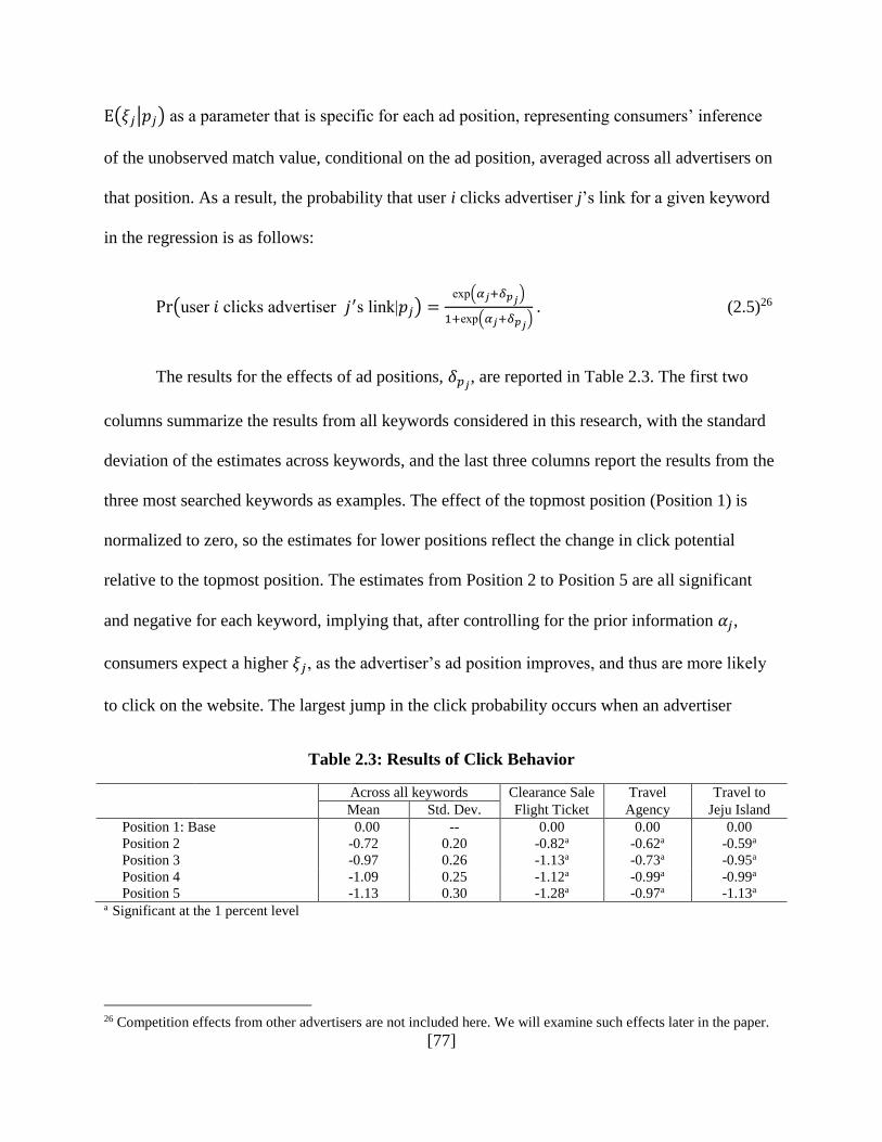
[77]

E(𝜉𝑗|𝑝𝑗) as a parameter that is specific for each ad position, representing consumers’ inference

of the unobserved match value, conditional on the ad position, averaged across all advertisers on

that position. As a result, the probability that user i clicks advertiser j’s link for a given keyword

in the regression is as follows:

Pr(user 𝑖 clicks advertiser 𝑗′s link|𝑝𝑗) =exp(𝛼𝑗+𝛿𝑝𝑗

)

1+exp(𝛼𝑗+𝛿𝑝𝑗) . (2.5)26

The results for the effects of ad positions, 𝛿𝑝𝑗, are reported in Table 2.3. The first two

columns summarize the results from all keywords considered in this research, with the standard

deviation of the estimates across keywords, and the last three columns report the results from the

three most searched keywords as examples. The effect of the topmost position (Position 1) is

normalized to zero, so the estimates for lower positions reflect the change in click potential

relative to the topmost position. The estimates from Position 2 to Position 5 are all significant

and negative for each keyword, implying that, after controlling for the prior information 𝛼𝑗,

consumers expect a higher 𝜉𝑗, as the advertiser’s ad position improves, and thus are more likely

to click on the website. The largest jump in the click probability occurs when an advertiser

Table 2.3: Results of Click Behavior



Position 1: Base 0.00 -- 0.00 0.00 0.00

Position 2 -0.72 0.20 -0.82a -0.62a -0.59a

Position 3 -0.97 0.26 -1.13a -0.73a -0.95a

Position 4 -1.09 0.25 -1.12a -0.99a -0.99a

Position 5 -1.13 0.30 -1.28a -0.97a -1.13a a Significant at the 1 percent level

26 Competition effects from other advertisers are not included here. We will examine such effects later in the paper.

[78]

moves from Position 2 to Position 1. This result is consistent throughout all other analyses. To

conclude, our test results support Hypothesis 1.27


For the signaling theory to work, consumers should also be more likely to find the offering from

advertisers at higher ad positions a match. Under the assumption that terminal clicks are a good

measure for comparing matches, it is expected to find that advertisers at higher positions are

more adept at producing terminal clicks once consumers have clicked the link. To test this

hypothesis, we first look at the TCTR, unconditional on clicks, from the top to the bottom

position in the data. The lower panel of Table 2.2 shows that the higher the ad position the more

likely a sponsored link will be chosen as the terminal click during keyword search. Specifically,

the topmost position generates twice as many terminal clicks as the second position across the

keywords in this study. These patterns are also consistent when comparing the top three searched

keywords.

We further utilize the regression approach to test Hypothesis 2. From equations (1) to (3),

the consumer latent utility can be written as

𝑉𝑖𝑗 = 𝛼𝑗 + 𝜉𝑗 + 𝜔𝑖𝑗,

where 𝜔𝑖𝑗 ≡ 𝜐𝑖𝑗 + 𝑒𝑖𝑗. After clicking into a website, the consumer will terminate search if the

advertiser’s offering matches her needs; otherwise she will continue searching. Conditional on

27 There are additional issues, as 𝛼𝑗 may vary over time and lead to the change in the advertiser’s ad position. In this

case our estimated 𝛿𝑝𝑗 may be biased. Further, consumers may simply search in a non-strategic top-down manner.

Such behavior could also explain our results. We will investigate these issues in the next section when we examine

alternative explanations for the results.

[79]

the ad position pj, the probability that the link is a match implies that 𝑉𝑖𝑗 is larger than a threshold

(normalized to zero) is

Pr(user 𝑖 terminates search after clicking link j |𝑝𝑗) = Pr (𝑉𝑖𝑗≥0|𝑝𝑗) .

The signaling theory predicts that 𝑝𝑗 is monotonically increasing with 𝜉𝑗; therefore, we can

rewrite the above probability function as

Pr(user 𝑖 terminates search after clicking link j |𝑝𝑗) = Pr (𝛼𝑗 + 𝜉(𝑝𝑗) + 𝜔𝑖𝑗≥0), (2.6)

where 𝜉(𝑝𝑗) is a monotonically increasing function of the ad position.

We use a reduced-form regression to test the relationship between 𝜉𝑗 and pj. For the

identification of model estimation, we assume that 𝜔𝑖𝑗 has EV Type 1 distribution, and treat

𝜉(𝑝𝑗) as a position-specific parameter to be estimated. Therefore, probability function (2.6) is as

follows,

Pr(user 𝑖 terminates search after clicking link j |𝑝𝑗) =exp(𝛼𝑗+𝜉(𝑝𝑗))

1+exp(𝛼𝑗+𝜉(𝑝𝑗)) . (2.7)

Let Si be the set of links clicked by consumer i, and tij be an indicator function that is equal to 1

if the user terminates search after clicking link j, and 0 otherwise. At most one link from Si has tij

= 1 and, if none of the clicks are terminal clicks, we have ∑ 𝑡𝑖𝑗𝑗∈𝑺𝑖= 0. The conditional

likelihood of the choice of terminating clicks {𝑡𝑖𝑗; 𝑗 ∈ 𝑺𝑖} is

Pr(𝑡𝑖𝑗; 𝑗 ∈ 𝑺𝑖 |𝒑) = ∏ (exp(𝛼𝑗+𝜉(𝑝𝑗))

1+exp(𝛼𝑗+𝜉(𝑝𝑗)))

𝑡𝑖𝑗

×𝑗∈𝑺𝑖(1 −

exp(𝛼𝑗+𝜉(𝑝𝑗))

1+exp(𝛼𝑗+𝜉(𝑝𝑗)))

1−𝑡𝑖𝑗

, (2.8)

[80]

where p is the vector of all advertisers’ positions. Under this specification, the likelihood is the

product of binary logit probabilities, conditional on the set of links that have been clicked.28

Table 2.4 presents the estimation results. The negative estimates for 𝜉(𝑝𝑗) suggest that the ξ’s at

lower positions are lower than that for the top position, which is normalized to 0. Furthermore,

the lower the ad position the smaller the estimated 𝜉(𝑝𝑗), a monotonic relationship predicted by

the signaling theory. These results provide significant evidence supporting Hypothesis 2 and the

signaling prediction that advertisers at higher positions are more likely to match with consumers

than advertisers at lower positions.

Table 2.4: Results of Terminal Click Behavior



Position 1: Base 0.00 -- 0.00 0.00 0.00

Position 2 -0.18 0.22 -0.21b 0.16 -0.17c

Position 3 -0.25 0.25 -0.22b -0.29b -0.11

Position 4 -0.20 0.24 -0.24c -0.08 -0.24b

Position 5 -0.34 0.49 -0.15 0.08 -0.35b a Significant at the 1 percent level, b 5 percent, c 10 percent


We now test the relationship between an advertiser’s bid decision and the likelihood that its link

will match with a given consumer. As we have discussed before, advertisers in our data

frequently change bids for specific keywords but their ad positions could remain unchanged (i.e.,

they cannot outbid advertisers on top). The signaling theory predicts that, when an advertiser

28 A multinomial logit (MNL) model is not a correct specification. The implicit assumption of the MNL model is

that a consumer first clicks on a number of links and then determines which will be her terminal click. The main

issue is that if only one sponsored link is clicked, the likelihood that the link is a terminal link is 100% no matter

how estimates change; thus, this observation is non-informative for estimating the position effects. In our data most

of these consumers choose the top-positioned link. On the other hand, consumers who click multiple links typically

terminate their search at lower positions. This is because consumers often start searching at top positions and, if the

links are not a match, they will continue down the list and stop searching at lower positions. We estimate such a

model. Results show that, relative to the topmost position, lower-ranked positions are more likely to generate

terminal clicks, clearly inconsistent with the observations from Table 2.2.

[81]

increases its bid, it will generate more terminal clicks, while remaining at the same ad position,

as the bid increase reflects an increase in the match value unobserved to consumers (𝜉𝑗). The

consumer will be more likely to terminate her search with the advertiser because, after clicking

into the advertiser’s website, the consumer will be more likely to find a match.

We test the correlation between the TCTR of an advertiser and its bids. We construct

indicator variables for every advertiser-position combination in the data set, and then model

terminal click as a MNL decision out of all listed sponsored links for each search occasion. The

probability that user i chooses advertiser j at position l for the terminal click is as follows:

Pr(user 𝑖 terminal-clicks advertiser 𝑗′s link at position 𝑙) =exp(BID𝑖𝑗∙𝛽+𝛼𝑗𝑙)

1+∑ exp(BID𝑖𝑗′∙𝛽+𝛼𝑗′𝑙′)𝐽

𝑗′=1

, (2.9)

where 𝛼𝑗𝑙 is the fixed effect for advertiser j listed at position l, and 𝛼𝑗′𝑙′ is the fixed effect for

competing advertiser j’ at position l’. BID𝑖𝑗 is the bid amount of advertiser j for the keyword.

Terminal clicks for organic links, or no clicks at all, are the outside option, whose value is

captured by “1” in the denominator. We estimate 503 advertiser-position fixed effects in the

regression. If changing bid amounts leads to changing positions, the effect on terminal clicks is

captured by such fixed effects. The parameter 𝛽, therefore, is estimated from the variation in

advertisers’ bids which does not alter their positions. The reason that we choose the MNL

specification is because it controls for competitor effects, where other advertisers may also

increase bids and have an effect on the TCTR of advertiser j. Our estimation results show that 𝛽

is positive (0.56) and is significant at the 1% level. This indicates that an advertiser’s bid is

positively correlated with the TCTR, even when its ad position remains unchanged, providing

support for the first part of Hypothesis 3.

[82]

To test whether this positive correlation is due to some “macro shocks”, under which the

advertisers simultaneously increase (decrease) bid amounts, due to increased (decreased)

profitability from search advertising shared by everyone (e.g., advertisers may drop their bids at

night if fewer clicks at night convert to purchases), but remain in the same ad positions, we

further estimate another MNL model, allowing indicators for both the day of the month and the

time of the day as additional explanatory variables in the regression. In this robustness check, 𝛽

remains positive (0.63) and significant at the 1% level. The results are strong evidence

supporting the firm behaviors predicted by the signaling theory.

The second part of Hypothesis 3 states that the change in the advertiser’s bid decision is

not driven by the change in 𝛼𝑗, the part in the latent utility that consumers already know before

clicking into the advertiser’s website. If only 𝜉𝑗 changes, the CTR should not correlate with the

advertiser’s bid decision, since consumers do not observe how much each advertiser bids. To test

this hypothesis, we further run a “placebo” test by using a logit model to regress clicks, rather

than terminal clicks, against advertiser-position fixed effects and bid amounts. Our estimation

results show that the estimated 𝛽 is small in magnitude and statistically insignificant (𝛽 = 0.09,

p-value = 0.48). Therefore, when an advertiser increases its bid, but remains in the same position,

it is more likely to generate terminal clicks, but not more likely to generate clicks. Combining all

of these test results, it suggests that when advertisers increase their bids, it is not entirely due to

the change in their service offering that is known by consumers prior to clicking sponsored links.

They do so because of the improvement in the unknown match value, which they can signal

through their ad positions.

[83]

In total, these tests have provided evidence for the three main predictions of signaling

theory: consumers are more likely to click on advertisers in higher positions, consumers are more

likely to match with advertisers in higher positions, and when advertisers will increase their bids,

their offerings are more likely to match with consumers’ needs. In the next section we will

discuss a number of possible non-signaling explanations for these results.

2.5 Alternative Explanations

In section 4 we have established the key results to support that signaling theory is at work in our

empirical context. However, there may be other, non-signaling, explanations that lead to such

results. In this section we explore several key alternative explanations and show that they cannot

fully explain our findings. We do not argue that these factors do not affect consumer click

behaviors, or that signaling is the only explanation; instead, our goal is to test whether, despite

the existence of other factors, signaling match value plays a significant role in the search

advertising market.

2.5.1 Endogeneity due to External Factors

We have shown a positive relationship between the positions of advertisers and their CTR and

TCTR. Sponsored positions, however, are endogenously determined by the bidding decisions of

advertisers. Suppose advertisers engage in marketing activities (e.g., an ad campaign in radio or

on TV may increase consumers’ interest in the advertiser) that consumers know prior to clicking

into their websites but as researchers we do not observe. If advertisers also bid for higher

positions, this creates an endogeneity issue what can lead to biased results in the tests for

[84]

Hypotheses 1 and 2. Notice that if an advertiser participates in such activities that increase its

match value, and at the same time improves its ad position to send signals to consumers, this is

consistent with the signaling model. We differentiate between the activities of which consumers

are informed only via signaling from ad positions, and activities that do not rely on signaling. To

establish the signaling effect from search advertising, we have to control for the latter

explanation.

Results from testing Hypothesis 3 partly address such a concern, since they suggest that

advertisers’ bid decisions are not entirely driven by the activities that consumers already know.

This strategy of testing, however, relies on the observations in which the advertiser’s ad position

does not change with bids. What about the test results that are conditional on changes in ad

positions? To rule out that they are driven by the external factors that are observed by consumers

prior to clicking, we turn to the binary logit model in equation (2.5) that we use to test

Hypothesis 1, where we assume 𝛼𝑗 to be an advertiser-specific fixed effect. If the advertiser’s

external activities (as well as any other factors that impact consumer clicks) remain unchanged in

the data period, then the effect has been captured by 𝛼𝑗. The concern is that the advertiser effect

may change within the data period because of time-varying external factors. We use a unique

feature in our data to control for this possible explanation: on average, an advertiser in data is

placed in 2.4 (or 2 as the median) positions per day. We estimate the consumer click decision

with a binary logit model, but allow for unique advertiser-day fixed effects. This estimation will

separate out the effects from unobserved external factors that remain constant within a day from

the position effects. The latter effects can only be identified from those advertisers whose ad

positions have changed within a day. The results are presented in Table 2.5. We again find

significant position effects that are of roughly the same magnitude to those estimates presented in

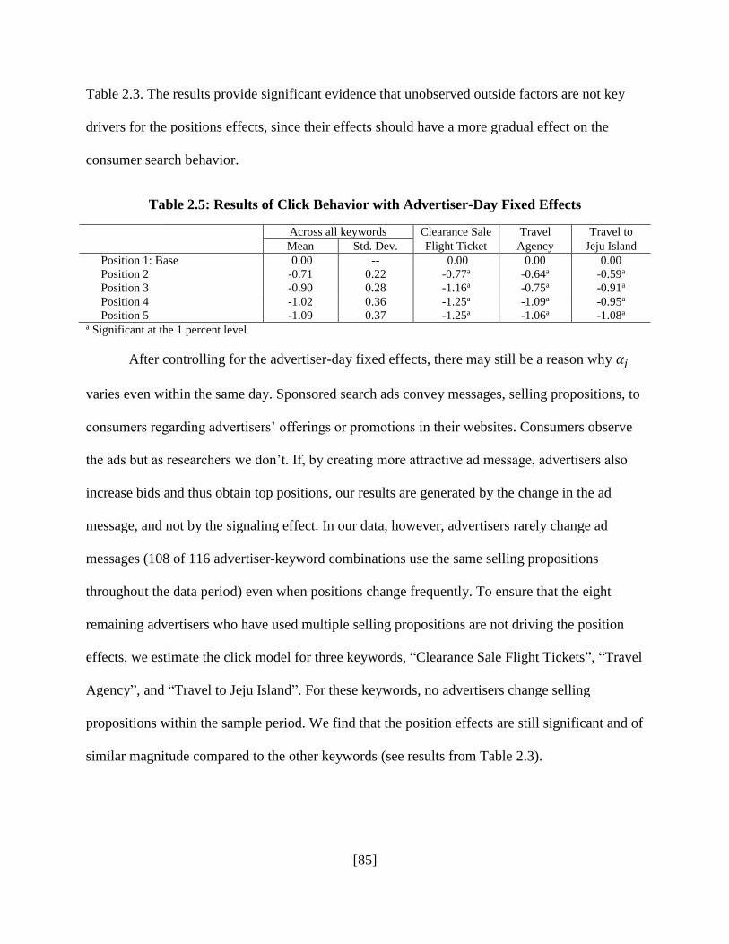
[85]

Table 2.3. The results provide significant evidence that unobserved outside factors are not key

drivers for the positions effects, since their effects should have a more gradual effect on the

consumer search behavior.

Table 2.5: Results of Click Behavior with Advertiser-Day Fixed Effects



Position 1: Base 0.00 -- 0.00 0.00 0.00

Position 2 -0.71 0.22 -0.77a -0.64a -0.59a

Position 3 -0.90 0.28 -1.16a -0.75a -0.91a

Position 4 -1.02 0.36 -1.25a -1.09a -0.95a


After controlling for the advertiser-day fixed effects, there may still be a reason why 𝛼𝑗

varies even within the same day. Sponsored search ads convey messages, selling propositions, to

consumers regarding advertisers’ offerings or promotions in their websites. Consumers observe

the ads but as researchers we don’t. If, by creating more attractive ad message, advertisers also

increase bids and thus obtain top positions, our results are generated by the change in the ad

message, and not by the signaling effect. In our data, however, advertisers rarely change ad

messages (108 of 116 advertiser-keyword combinations use the same selling propositions

throughout the data period) even when positions change frequently. To ensure that the eight

remaining advertisers who have used multiple selling propositions are not driving the position

effects, we estimate the click model for three keywords, “Clearance Sale Flight Tickets”, “Travel

Agency”, and “Travel to Jeju Island”. For these keywords, no advertisers change selling

propositions within the sample period. We find that the position effects are still significant and of

similar magnitude compared to the other keywords (see results from Table 2.3).

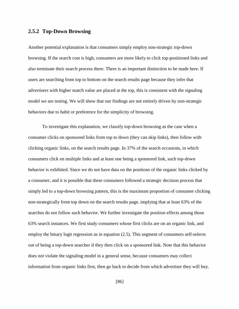
[86]

2.5.2 Top-Down Browsing

Another potential explanation is that consumers simply employ non-strategic top-down

browsing. If the search cost is high, consumers are more likely to click top-positioned links and

also terminate their search process there. There is an important distinction to be made here. If

users are searching from top to bottom on the search results page because they infer that

advertisers with higher match value are placed at the top, this is consistent with the signaling

model we are testing. We will show that our findings are not entirely driven by non-strategic

behaviors due to habit or preference for the simplicity of browsing.

To investigate this explanation, we classify top-down browsing as the case when a

consumer clicks on sponsored links from top to down (they can skip links), then follow with

clicking organic links, on the search results page. In 37% of the search occasions, in which

consumers click on multiple links and at least one being a sponsored link, such top-down

behavior is exhibited. Since we do not have data on the positions of the organic links clicked by

a consumer, and it is possible that these consumers followed a strategic decision process that

simply led to a top-down browsing pattern, this is the maximum proportion of consumer clicking

non-strategically from top down on the search results page, implying that at least 63% of the

searches do not follow such behavior. We further investigate the position effects among those

63% search instances. We first study consumers whose first clicks are on an organic link, and

employ the binary logit regression as in equation (2.5). This segment of consumers self-selects

out of being a top-down searcher if they then click on a sponsored link. Note that this behavior

does not violate the signaling model in a general sense, because consumers may collect

information from organic links first, then go back to decide from which advertiser they will buy.

[87]

Bentley et al. (2015) study why, when there are uncertainties for the keyword and advertisers’

offerings, consumers may search organic results before clicking sponsored links, and how the

Table 2.6: Results of Click Behavior with First Clicks Being on Organic Links



Position 1: Base 0.00 -- 0.00 0.00 0.00

Position 2 -.055 0.30 -0.73a -0.45a -0.47a

Position 3 -0.71 0.20 -1.00a -0.59a -0.72a

Position 4 -0.86 0.21 -1.07a -0.78a -0.74a


information from organic results impacts the probability of clicking sponsored links. Table 2.6

presents the regression results. The position effects are still significant, similar to our previous

findings. These cannot be explained by the top-down browsing behavior.

To further investigate the explanation of top-down browsing behavior, we estimate two

additional models in which consumers select out of top-down browsing. First, we estimate the

model conditional on observations in which consumers first click on the fifth (last) sponsored

link. Very few consumers do so (1,124 out of 128,473 search instances), and even fewer follow

up by clicking more sponsored links. Because of the lack of observations, we pool all keywords

in the estimation and only focus on the effect from the top position. The estimated coefficient is

0.34 (the effects of lower-positions are normalized to zero), significant at the 1% level,

indicating that the topmost position attracts more clicks than all other positions that are above the

fifth link. We also estimate the model conditional on the first click being at any sponsored link

lower than the topmost position. Again, we only estimate the effect from the topmost position,

while normalizing the effects from all lower positions to be zero. Once again we find a

significant positive top rank effect (0.19 at the 5% level). Both results provide further evidence

[88]

that the non-strategic top down behavior is not the sole driver of the results in our empirical

context.

2.5.3 Persuasive Function

Another potential driver of our results on the signaling theory is persuasion in advertising. The

signaling model suggests that consumers believe that advertisers with high match value are more

likely to occupy high ad positions. In a broad sense, the persuasion explanation is consistent with

such a model. The alternative explanation we investigate here is that the consumer belief is not

rational, as advertisers with lower match value outbid advertisers with higher match value to gain

clicks and sales from consumers who follow the belief. Jerath et al. (2011) offer a possible

explanation why such bidding strategy is an equilibrium outcome and rationalize the so-called

“Position Paradox”. They assume that uninformed consumers follow a top-down search strategy

which, in some occasions, may not be optimal given advertisers’ bidding strategy, while

informed consumers begin their search with the superior firm regardless of ad position in

sponsored listing. Our goal is to test whether our findings are only driven by this pure persuasive

advertising explanation.

Suppose consumers’ expectation is not consistent with advertisers’ bidding strategy. In

such case, it is expected to find TCTR not to be positively correlated with the ad position. This is

inconsistent with our findings when testing Hypothesis 2. A potential counter-argument is that,

suppose search is costly for consumers. Consumers are more likely to stop searching after

clicking top positions. However, this argument cannot explain our findings when testing

Hypothesis 3. There should be no reasons that the TCTR increases with increasing bids from

advertisers, when their ad positions remain constant. Also, since the CTR does not change (as we

[89]

have shown in the “placebo” test) in this scenario, the persuasion function of ad positions does

not seem to have improved. Therefore, the tests for Hypotheses 2 and 3 show that our findings

are not solely driven by the pure persuasive function of ad positions.

We follow up with another test comparing the position effects across keywords. There are

some “general” keywords that consist of multiple product or service offerings (e.g., “Flight

Ticket” consists of flights to different destinations), and multiple attributes for the offerings (e.g.,

“Flight Ticket” consists of not only prices but also departure and arrival places and flight

schedules), that consumers care about. For these keywords, the offerings from an advertiser may

be a good match for some consumers but not for the others. The markets are therefore more

horizontally differentiated. In contrast, there are “focused” keywords that are restricted to

specific product or service offerings (e.g., “Flight Ticket to Jeju Island” focuses on a single

destination) or attributes (e.g., “Clearance Sales Flight Ticket” targets consumers looking for low

prices). For such keywords, the needs and preferences of consumers are well defined and less

heterogeneous. The difference can be illustrated from equation (2.3). The magnitude of the

variance of 𝜉’s across advertisers, relative to the magnitude of the variance of 휀’s across

individual consumers and advertisers, should be larger for focused keyword than for general

keywords. For focused keywords, advertisers with high 𝜉’s have a larger likelihood that their

offerings match the needs and preferences of individual consumers who click at their sponsored

links, so they are more likely to bid higher than advertisers with low 𝜉’s. Knowing this, rational

consumers are also more likely to click on high-positioned sponsored links. The signaling

function thus is stronger for focused keywords than general keywords. If our findings are only

driven by persuasive advertising, however, there should not be any difference between “general”

[90]

keywords and “focused” keywords regarding the advertiser and consumer behaviors, as

consumers would not be rationally inferring advertisers’ bidding incentives.

We compare four pairs of keywords in which the first keyword in the pair is more general

than the second, which is more focused, as follows:

1. “Flight Ticket” vs. “Flight Ticket to Jeju Island”

2. “Travel to Jeju Island” vs. “Flight Ticket to Jeju Island”

3. “Travel Agencies” and “Price Comparison of Travel Agencies”

4. “Flight Ticket” and “Clearance Sale Flight Ticket”

“Flight Ticket to Jeju Island” is similar to “Flight Ticket” without the variety of destinations,

“Flight Ticket to Jeju Island” is a specific travel mode of "Travel to Jeju Island,” “Price

Comparison of Travel Agencies” narrows down the attributes of interest for “Travel Agencies”

to price, as does “Clearance Sale Flight Ticket” when compared to “Flight Ticket.”

We run a binary logit model of consumer clicks to estimate the position effects for

general keywords, and the differences in the effects between the two types of keywords for each

ad position. The coefficient for the top position is normalized to zero, so a negative coefficient

for the differences will mean that the signaling effect (of top position, relative to lower positions)

is stronger for focused keywords. Table 2.7 shows the results. All coefficients are negative, with

the majority being significant. These results offer further evidence that the persuasive effect

cannot fully explain our findings. Yet the signaling theory can rationalize why there are

differences between keywords.

[91]

Table 2.7: Results of Click Behavior with

Differences in Position Effects between General and Focused Keywords

Keyword Pairs

1 2 3 4

General keywords Flight Ticket Travel to Jeju Island Travel Agencies Flight Ticket

Focused keywords Flight Ticket to

Jeju Island

Flight Ticket to

Jeju Island

Price Comparison of

Travel Agencies

Clearance Sale

Flight Ticket

Position 1: Base 0.00 0.00 0.00 0.00

Position 2 -0.12 -0.25b -0.46a -0.11

Position 3 -0.31b -0.19 -0.72a -0.32a

Position 4 -0.43a -0.30b -0.58a -0.34a

Position 5 -0.31c -0.13 -0.77a -0.29b a Significant at the 1 percent level, b 5 percent, c 10 percent

2.5.4 Informative Function

Another important role of advertising identified in the literature is the informative function.

Broadly speaking, the signaling function of advertising is also informative to consumers

regarding the match value of advertisers. We examine here the narrow definition of the

informative function, i.e., the selling proposition in an advertisement informs consumers about

the existence of the advertiser’s website, prices, and product or service offerings that affects

consumers’ click and purchase decisions.

If an ad in sponsored listing is to inform consumers of the advertiser’s website, there is

no reason why top positions will get more clicks than lower positions, assuming that consumers

browse all sponsored links before clicking. If consumers browse top-down and decide whether

they will click each sponsored link sequentially, the advertiser at the top position may generate

more clicks. However, our previous tests, using observations in which consumers click organic

links first and click lower positions first, do not support this argument. Therefore, we can rule

out that our findings of the position effects are driven by the informative function of search

advertising on the consumer awareness. Furthermore, since we have included advertiser fixed

[92]

effects when testing Hypothesis 1, the position effects we have identified could be driven by the

changes in selling propositions within advertisers. As we have shown in Section 5.1 when

investigating the alternative explanation that the advertiser effects may be time-varying,

advertisers rarely change ad messages even when positions change frequently. We also find that

the position effects are still significant for the three keywords of which selling propositions have

never changed. Therefore, the position effects we have documented are not driven by the

informative function.

2.6 Spillover Effects of Advertising

We study in this section how the CTR of a sponsored link is influenced by competing sponsored

links, and show the existence of an information externality that is consistent with the signaling

framework. In search advertising, sponsored ads appear so that consumers can navigate through

listings to search for information. The advertisement from an advertiser with good offerings may

send a positive signal about the match value of other sponsored links. Jeziorski and Segal (2014)

suggest that “such updating would generate positive informational externalities across ads, i.e.,

an ad would benefit from having better ads in the same impression.” On the other hand, such an

advertiser will also attract consumers searching its website first and thus may reduce the

likelihood of clicking other sponsored links, creating a competitive effect. Which effect

dominates the other one is an important empirical question for online advertisers as well as

search engines.

The phenomenon of the “informational externality” can be rationalized via the signaling

model. In the model of Athey and Ellison (2011), consumers update the expected value for the

[93]

’s for the links that have not been clicked, conditional on the revealed ’s from links that have

been clicked, as well as the positions of all links, in a Bayesian way. Consider searching the

keyword “Travel to Jeju Island” returns two sponsored links. Let the match value 𝜉’s be

distributed uniformly from 0 to 1, with 1 being the highest possible value. Suppose a consumer

finds that the average match value of the advertiser at the top position is high at 0.8 (e.g., the

advertiser offers low prices for packaged tours to Jeju Island) but nothing matches with her

specific needs (e.g., there are no tours on the dates she wants to travel). Based on the information

of the match value of the advertiser, the consumer will infer the match value of the advertiser

below is between 0 and 0.8, with the updated expectation equal to 0.4. She may continue her

search by clicking the sponsored link below. If, instead, the average match value of the top

advertiser is 0.2, the consumer will infer that the average match value of the advertiser below is

between 0 and 0.2 with the updated expectation at 0.1. The consumer may be more likely to

terminate her search after clicking the sponsored link at the top. This suggests that the existence

of an advertiser with high match value may increase the number of clicks that a competing

advertiser obtains, creating a “market expansion” effect, i.e., increasing the number of consumers

who clicks sponsored links. Competition of course is also important. If most consumers, after

first searching the website of the advertiser at the top, find a match and thus terminate the search,

the advertiser below will not get additional clicks. In this case the negative competitive effect

dominates the positive informational externality.

We use two ways to test the magnitude of the spillover effects. We first use the binary

logit model from equation (2.5) but modify as follows:

Pr(user 𝑖 clicks advertiser 𝑗′s link) =exp(𝛼𝑗+𝛿𝑝𝑗

+SPILLOVER𝑖𝑗∙𝛾)

1+exp(𝛼𝑗+𝛿𝑝𝑗+SPILLOVER𝑖𝑗∙𝛾)

, (2.10)

[94]

where SPILLOVER𝑖𝑗 is a measure of the match value of all other advertisers above and below

advertiser j’s ad position for a given keyword, and 𝛾 is a set of parameters that captures the net

spillover effects. The regression controls for the advertiser fixed effects, 𝛼𝑗, and the position

effect, 𝛿𝑝𝑗. SPILLOVER𝑖𝑗 is specified as a function of {𝛼𝑘, for all 𝑘 ≠ 𝑗}, the set of all

advertisers competing with advertiser j on the search results page. We estimate the above model

with three specifications for SPILLOVER𝑖𝑗 . The first specification (“Mean”) takes the average

of the estimated fixed effects from competing advertisers, from advertisers positioned above

(zero for the topmost position) and positioned below (zero for the lowest position). The second

specification (“Max”) takes the advertiser, positioned above and below, with the highest fixed

effect. For the third specification (“Percent”), we calculate for a specific advertiser the

percentage of advertisers who have a higher fixed effect, positioned above and below.

Since the click probability of each advertiser depends on not only its own fixed effect but

also the fixed effects from advertisers at other ad positions, we estimate all advertiser fixed

effects simultaneously through equation (2.10) for all of the advertisers. Results are reported in

Table 2.8. For each specification, an increase in the match value of higher positioned advertisers

will increase the click potential for a given advertiser, significant at the 1% level. In the Mean

and Max specifications, we also find a positive spillover effect from lower-positioned

advertisers, significant at the 10% and 5% level, respectively. Since the estimates represent the

combined spillover effects and competitive effects, and because the latter is a negative effect,

these results suggest that the positive information externalities from high-match value

competitors are strong in the search advertising context.

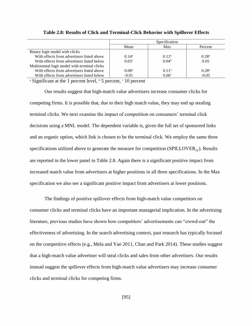
[95]

Table 2.8: Results of Click and Terminal-Click Behavior with Spillover Effects

Specification

Mean Max Percent

Binary logit model with clicks

With effects from advertisers listed above 0.14a 0.12a 0.28a

With effects from advertisers listed below 0.03c 0.04b 0.05

Multinomial logit model with terminal clicks

With effects from advertisers listed above 0.08a 0.11a 0.28a

With effects from advertisers listed below -0.01 0.06c -0.05 a Significant at the 1 percent level, b 5 percent, c 10 percent

Our results suggest that high-match value advertisers increase consumer clicks for

competing firms. It is possible that, due to their high match value, they may end up stealing

terminal clicks. We next examine the impact of competition on consumers’ terminal click

decisions using a MNL model. The dependent variable is, given the full set of sponsored links

and an organic option, which link is chosen to be the terminal click. We employ the same three

specifications utilized above to generate the measure for competition (SPILLOVER𝑖𝑗). Results

are reported in the lower panel in Table 2.8. Again there is a significant positive impact from

increased match value from advertisers at higher positions in all three specifications. In the Max

specification we also see a significant positive impact from advertisers at lower positions.

The findings of positive spillover effects from high-match value competitors on

consumer clicks and terminal clicks have an important managerial implication. In the advertising

literature, previous studies have shown how competitors’ advertisements can “crowd-out” the

effectiveness of advertising. In the search advertising context, past research has typically focused

on the competitive effects (e.g., Mela and Yao 2011, Chan and Park 2014). These studies suggest

that a high-match value advertiser will steal clicks and sales from other advertisers. Our results

instead suggest the spillover effects from high-match value advertisers may increase consumer

clicks and terminal clicks for competing firms.

[96]

2.7 Conclusions

In this paper, we test the empirical validity of the signaling theory of advertising in the search

advertising context. By using detailed data of travel-related keywords which are obtained from a

search engine, we have tested a series of predictions both on consumer and advertiser behaviors

in accordance to the signaling theory of advertising. We have shown that consumers are more

likely to not only click on an advertiser listed at higher positions but also terminate their search

at such link. On the advertiser side, we find that the increase in terminal clicks is positively

correlated with the increase in advertisers’ bid amounts, even when ad positions remain

unchanged. However, there is no increase in CTR. In sum, our empirical results support

predictions from the signaling theory of advertising in the literature. Additionally, we have

controlled for several key alterative explanations for how search advertising works, and find that

our results still hold. Finally, we find that advertisers can generate more clicks and terminal

clicks when competing against advertisers with higher match value, due to an information

externality. This finding can be explained based on the signaling theory.

Our application has two important limitations that should be addressed by further

research. First, we focus on a dataset of travel-related keywords to empirically test the signaling

theory in the search advertising context. We chose the travel category because consumers have

uncertainty regarding the attributes of products or services they search and their searches are

costly in such experience goods markets with differentiated products or services. This means our

conclusions may not generalize to other settings. Future work can build on our approaches and

findings by analyzing other types of keywords and/or obtained from other sources, which can

[97]

possibly lead to the empirical generalization regarding the relevance of the signaling theory in

advertising. Second, we used terminal clicks to proxy whether an advertiser’s offering is a match

for consumer needs, because our data did not include post-conversion behavior. The availability

of data on post-click conversion rates can further enhance our understanding of consumer

behavior. By the same token, the availability of data on advertisers’ other types of marketing

activities can help study the signaling theory in a broader advertising context. We hope that this

study demonstrates the efficacy of the signaling theory and can motivate further research in the

contexts where both consumers and advertisers strategically behave when uncertainty exists.

[98]

2.8 References

Agarwal, A., K. Hosanagar and M. Smith (2011), “Location, Location, Location: An Analysis of

Profitability of Position in Online Advertising Markets,” Journal of Marketing Research, 48

(6), 1057-1073.

Agarwal, N., S. Athey and D. Yang (2009), “Skewed Bidding in Pay per Action Auctions for

Online Advertising,” American Economic Review: Papers & Proceedings, 99 (2), 441-447.

Anderson, S., and R. Renault (2006), “Advertising Content,” American Economic Review, 96

(1), 93-113.

Athey, S., and G. Ellison (2011), “Position Auctions with Consumer Search,” Quarterly Journal

of Economics, 126 (3), 1213-1270.

Athey, S., and D. Nekipelov (2012), “A Structural Model of Sponsored Search Advertising

Markets,” Working Paper, Stanford University.

Bagwell, K., and M. Riordan (1991), “High and Declining Prices Signal Product Quality,”

American Economic Review, 81 (1), 224-239.

Bentley, T., T. Chan and Y.-H. Park (2015), “How Search Advertising Works? A Model of

Consumer Information Search in Informational and Seller Links,” Working Paper,

Washington University in St. Louis.

Caves, R., and D. Greene (1996), “Brands’ Quality Levels, Prices, and Advertising Outlays:

Empirical Evidence on Signals and Information Costs,” International Journal of Industrial

Organization, 14 (1), 29-52.

[99]

Chan, T., and Y.-H. Park (2014), “The Value of Consumer Search Activities for Sponsored

Search Advertisers,” Marketing Science, forthcoming.

Chen, Y., and C. He (2011), “Paid Placement: Advertising and Search on the Internet,”

Economic Journal, 121 (56), F309-F328.

De Los Santos, B., A. Hortacsu, and M. Wildenbeest (2012), “Testing Models of Consumer

Search Using Data on Web Browsing and Purchasing Behavior,” American Economic

Review, 102 (6), 2955-2980.

Edelman, B., and M., Ostrovsky (2007), “Strategic Bidder Behavior in Sponsored Search

Auctions,” Decision Support Systems, 43 (1), 192-198.

Edelman, B., M. Ostrovsky and M. Schwarz (2007), “Internet Advertising and the Generalized

Second Price Auction: Selling Billions of Dollars Worth of Keywords,” American Economic

Review, 97 (1), 242-259.

Feng, J., H. Bhargava and D. Pennock (2007), “Implementing Sponsored Search in Web Search

Engines: Computational Evaluation of Alternative Mechanisms,” INFORMS Journal on

Computing, 19 (1), 137-148.

Ghose, A., and S. Yang (2009), “An Empirical Analysis of Search Engine Advertising:

Sponsored Search in Electronic Markets,” Management Science, 55 (10), 1605-1622.

Goldfarb, A., and C. Tucker (2011), “Search Engine Advertising: Channel Substitution When

Pricing Ads to Context,” Management Science, 57 (3), 458-470.

[100]

Grossman, G., and C. Shapiro (1984), “Informative Advertising with Differentiated Products,”

Review of Economic Studies, 51 (1), 63-81.

Honka, E., and P. Chintagunta (2014), “Simultaneous or Sequential? Search Strategies in the

U.S. Auto Insurance Industry,” Working Paper, University of Texas, Dallas.

Jeziorski, P., and I. Segal (2014), “What Makes Them Click: Empirical Analysis of Consumer

Demand for Search Advertising,” Working Paper, Stanford University.

Jerath, K., L. Ma, and Y.-H. Park (2014), “Consumer Click Behavior at a Web Search Engine:

The Role of Keyword Popularity,” Journal of Marketing Research, 51 (4), 480-486.

Jerath, K., L. Ma, Y.-H. Park and K. Srinivasan (2011), “A ‘Position Paradox’ in Sponsored

Search Auctions,” Marketing Science, 30 (4), 612-627.

Kirmani, A. (1990), “The Effect of Perceived Advertising Costs on Brand Perceptions,” Journal

of Consumer Research, 17 (2), 160-171.

Kirmani, A., and P. Wright (1989), “Money Talks: Perceived Advertising Expense and Expected

Product Quality,” Journal of Consumer Research, 16 (3), 344-353.

Kim, J., P. Albuquerque, and B. Bronnenberg (2010), “Online Demand Under Limited

Consumer Search,” Marketing Science, 29 (6), 1001-1023.

Klein, B., and K. Leffler (1981), “The Role of Market Forces in Assuring Contractual

Performance,” Journal of Political Economy, 89 (4), 615-664.

McCall, J. (1970), “The Economics of Information and Job Search,” Quarterly Journal of

Economics, 84 (1), 113-126.

[101]

Meurer, M., and D. Stahl II (1994), “Informative Advertising and Product Match,” International

Journal of Industrial Organization, 21 (1), 1-19.

Milgrom, P., and J. Roberts (1986), “Price and Advertising Signals of Product Quality,” Journal

of Political Economy, 94 (4), 796-821.

Moorthy, S., and S. Hawkins (2005), “Advertising Repetition and Quality Perception,” Journal

of Business Research, 58 (3), 354-360.

Narayanan, S., and K. Kalyanam (2014), “Position Effects in Search Advertising: A Regression

Discontinuity Approach,” Working Paper, Stanford University.

Nelson, P. (1970), “Information and Consumer Behavior,” Journal of Political Economy, 78 (2),

311-329.

Nelson, P. (1974), “Advertising as Information,” Journal of Political Economy, 82 (4), 729-754.

Rutz, O., and R. Bucklin (2011), “From Generic to Branded: A Model of Spillover in Paid

Search Advertising,” Journal of Marketing Research, 48 (1), 87-102.

Stigler, G. (1961), “The Economics of Information,” Journal of Political Economy, 69 (3), 213-

225.

Tellis, G., and C. Fornell (1988), “Advertising and Quality Over the Product Life Cycle: A

Contingency Theory,” Journal of Marketing Research, 15 (1), 64-71.

Thomas, L., S. Shane and K. Weigelt (1998), “An Empirical Examination of Advertising as a

Signal of Product Quality,” Journal of Economic Behavior & Organization, 37 (4), 415-430.

[102]

Varian, H. (2007), “Position Auctions,” International Journal of Industrial Organization, 25 (6),

1163-1178.

Weitzman, M. (1979), “Optimal Search for the Best Alternative,” Econometrica, 47 (3), 641-

654.

Yang, S., and A. Ghose (2010), “Analyzing the Relationship Between Organic and Sponsored

Search Advertising: Positive, Negative, or Zero Interdependence?,” Marketing Science, 29

(4), 602-623.

Yao, S., and C. Mela (2011), “A Dynamic Model of Sponsored Search Advertising,” Marketing

Science, 30 (3), 447-468.

[103]

Chapter 3

Solving the Similarity and Dominance

Problems: The Elimination-by-Aspects

(EBA) Demand Model for Differentiated

Products

3.1 Introduction

“The EBA functional form has considerable potential for econometric applications” – Daniel

McFadden (1981)

The logit model is used with aggregate scanner data to model brands’ market shares as

functions of their marketing variables. However, the logit suffers from an undesirable

mathematical property called Independence from Irrelevant Alternatives (IIA), which creates two

adverse behavioral consequences, called similarity and dominance problems. The similarity

problem is the following: Suppose a brand (Milky Way) cuts its price at a store this week. One

would expect this price cut to disproportionately, and adversely, impact the market shares of

brands that are perceived to be more similar (Snickers) to the focal brand in terms of underlying

characteristics, rather than the market shares of brands that are perceived to be less similar

(Skittles) to the focal brand. The logit cannot handle this asymmetric impact of price cuts.

In order to solve the similarity problem, three alternative models of brands’ market shares

have been proposed in the literature: probit, nested logit and mixed logit. However, none of these

[104]

three models is well designed to satisfactorily handling the similarity problem. Their deficiencies

in this regard are given below.

1. The probit accommodates only pair-wise inter-brand similarities which severely

restricts the range of similarity structures that the probit can handle,

2. The nested logit, unlike the probit, can handle a broad range of inter-brand similarity

structures, but imposes a long menu of alternative tree structures that need to be

estimated, which renders the nested logit practically infeasible,

3. The mixed logit can handle flexible similarity structures (unlike the probit) and is also

practically wieldy (unlike the nested logit), but it is not theoretically well grounded as

a model of individual consumer choice. Furthermore, the continuous mixed logit, just

like the probit, can only accommodate pair-wise inter-brand similarities.

To the extent that flexibly accounting for similarity patterns in demand in a behavior-

theoretic manner is necessary to obtain superior empirical predictions of brands’ market share

changes in response to changes in brands’ marketing variables, the above-mentioned deficiencies

of existing models is troubling. Further, and even more importantly, none of the above models

can handle the dominance problem. The dominance problem is the following: Suppose a

dominated brand (i.e., one whose price and quality are both simultaneously worse than at least

one existing brand) is introduced to a market. Such a brand would not be expected to steal any

market share from existing brands. The probit, nested logit and mixed logit cannot satisfactorily

handle this either.

Therefore, a satisfactory modeling solution to the similarity and dominance problems is

called for in market share models. In this paper, we propose a closed-form market share model

that, in fact, offers this solution. Our model is called the Elimination-By-Aspects (EBA) demand

[105]

model for differentiated products. This model relies on the specification of shared aspects among

brands to flexibly account for similarity and dominance effects in demand. The shared aspects

represent not just pair-wise inter-brand similarities (as in the probit) but also all possible higher

orders (triple-wise, quarter-wise etc.) of similarities. These shared aspects also end up rendering

our proposed demand model immune to the Invariant Proportion of Substitution (IPS) restriction

that the probit, nested logit and mixed logit all additionally suffer from (Steenburgh 2008). In our

proposed demand model, aspect similarity among brands plays a central role in explaining shifts

in market share among brands in response to relative changes in the marketing mix. This feature

is critical while employing a demand model for differentiated products. This modeling flexibility

presents the potential for profit-improving marketing mix prescriptions for brand managers and

retailers. Using scanner data from 9 product categories, we show that this EBA model

outperforms the mixed logit and probit models in terms of in-sample fit and holdout predictions.

We also show that the retailer can improve gross profits up to 34.4% from pricing based on this

EBA model rather than the mixed logit model (which is generally, but wrongly, regarded as the

most flexible way of addressing similarity and dominance problems in demand). We expand on

these issues in the next section.

3.2 Modeling Brand-Level Market Shares

The logit model is a commonly used predictive model of demand for brands. The theoretical

roots of the logit model can be traced to the Luce choice axiom (Luce 1958) and some early

empirical applications of the logit model in marketing used the logit model to specify market

shares of brands as functions of their marketing variables (e.g., Nakanishi, Cooper and

[106]

Kassarjian 1974, Malhotra 1984 etc.). With the advent of new industrial organization methods in

recent years, the logit model has increasingly become the workhorse model of aggregate demand

for differentiated products for empirical economists and marketing researchers alike (see, for

example, Berry, Levinsohn and Pakes 1995, Sudhir 2001 etc.).

Despite its wide use and predictive ability, the logit model suffers from the undesirable

IIA property (Debreu 1960). An adverse consequence of the IIA property is called the similarity

problem: If a new brand (e.g., Ralph Nader) were introduced to the market (e.g., Presidential

Election), the logit model would imply that the new brand would steal market shares from

existing brands (e.g., George W. Bush and Al Gore) in direct proportion to their existing market

shares (poll numbers). In reality, however, one would expect the new brand (Nader) to steal

greater market share from an existing brand that is relatively similar (Gore) to the new brand

than from an existing brand that is relatively dissimilar (Bush). Addressing the similarity

problem, therefore, warrants the use of a predictive model of market shares that explicitly

accounts for inter-brand similarities.

A predictive model of market shares that accounts for pair-wise inter-brand similarities is

the probit, whose theoretical roots can be traced to Thurstone (1927), which allows for pair-wise

(asymmetric) correlations among brands’ market shares using a correlated random utility

framework. However, the probit model is computationally more difficult to estimate than the

logit model. Further, it can only handle inter-brand similarities among pairs (and not triples,

quartets etc.) of brands, which restricts its modeling flexibility in addressing the similarity

problem. This especially becomes a concern in a situation where three or more brands may share

a relevant aspect (for example, in the soda category, multiple brands share the “cola”

[107]

characteristic). That said, the probit has been shown to have superior predictive ability

comparted to the logit (e.g., Chintagunta 2001).

Another predictive model of market shares that accounts for inter-brand similarities is the

nested logit, first developed by Ben-Akiva (1973) and then derived as a special case of the

Generalized Extreme Value (GEV) model by McFadden (1978). This model groups brands into

different groups, such that relatively similar brands occupy the same group, while relatively

dissimilar brands fall within different groups. This form allows substitutability among brands

within the same group to be higher than substitutability among brands in different groups. Just

like the logit, the nested logit has an analytical closed-form, making it easy to estimate.

However, the nested logit requires a postulated tree-structure as the process model governing the

grouping of brands by consumers. Since the number of possible tree structures that can be

postulated increases in a rapidly convex manner with the number of brands in the category, the

estimation of the nested logit becomes computationally impractical with aggregate scanner data

that typically involve many (>5) brands. With 5 brands, for example, even assuming a one-stage

hierarchy, there are 25 - 1 = 31 possible trees with 2 groups, 35 – 1 - 93 = 149 possible trees with

3 groups and so on. For this reason, researchers have almost never used the nested logit to model

market shares of brands. A few exceptions are Goldberg (1995) and Sudhir (2001), both of

whom estimate the nested logit model, and Hui (2004) who estimates a generalized extreme

value model. However, these market share models are all based on specifically assumed, rather

than endogenously estimated, product characteristics and tree structures. Typically one does not

know what the correct tree structure is, which makes this approach unsatisfactory from an

application standpoint.

[108]

A third predictive model of market shares that accounts for inter-brand similarities is the

mixed logit (McFadden and Train 2000), which postulates a population mixture representation of

unobserved heterogeneity in the parameters of the logit across consumers. When applied to

aggregate market share data, the mixed logit resembles the probit in that the correlated brand

intercepts of the mixed logit are like the correlated error terms of the probit. Furthermore, the

mixed logit additionally allows for randomness in the remaining utility parameters, e.g.,

marketing mix coefficients. The mixed logit can be shown to approximate the choice

probabilities from any discrete choice model derived from random utility maximization

(McFadden and Train 2000). This study has led to the singular use of the mixed logit in

economics and marketing over the past 14 years as the appropriate market share model to

address IIA issues (e.g., Sudhir 2001). However, there is a major theoretical limitation to the

mixed logit. Unlike the probit and nested logit, it theoretically relaxes the similarity problem at

the population level and not at the individual consumer level. Instead, if one directly views the

mixed logit to be a model of individual consumer choice, the mixed logit does not have a natural

theoretical interpretation as does the logit, probit or nested logit. In other words, the mixed logit

is not a theoretically well specified model of individual consumer behavior.

3.2.1 The Dominance Problem

A second adverse consequence of the IIA property is called the dominance problem: in the

presidential election example of the previous section, suppose a new brand (e.g., Donald Trump)

were introduced to the market that is perfectly dominated by one of the existing brands (Bush) in

terms of product characteristics, that is, Bush offers a bundle of characteristics (e.g.,

“conservative values”) to the market that is no worse than the bundle of characteristics offered

[109]

by Trump and is at least better on one characteristic (say, “relevant executive experience as state

governor”). This new brand, then, would be expected to steal no market share from the existing

brands (Bush and Gore), leaving their market shares unchanged. However, if Trump entered the

market solely against Gore, Trump would be expected to steal market share in a magnitude

similar to that of Bush. The logit model would, however, wrongly imply that the new brand

would steal market shares from existing brands in direct proportion to their existing market

shares (poll numbers). The nested logit also cannot handle the dominance problem, but the mixed

logit can (as we will show using numerical examples in the next section).

A behavioral phenomenon that is an extreme manifestation of the dominance problem is

called the attraction problem (also called asymmetric dominance or decoy effect), where the

introduction of the dominated brand (Trump) increases the market share of an existing,

dominating brand (Bush). This effect has been documented in choice data from laboratory

experiments (Huber, Payne and Puto 1982, Huber and Puto 1983). None of the existing market

share models is designed to handle the attraction problem (see Malkoc, Hedgcock and Hoeffler

2013 for a good review).

3.2.2 Contribution of Research

In this research, we propose a model of brand-level market shares that flexibly solves the

similarity and dominance problems associated with existing models by explicitly allowing for all

possible shared aspects among all pairs, triples, quartets etc. of brands. Our model is called the

Elimination-By-Aspects (EBA) demand model for differentiated products. This model relies on

the specification of shared aspects among brands to flexibly account for similarity and

dominance effects in demand. The model extends Tversky’s (1972) EBA model for

[110]

differentiated products to handle time-varying covariates. The model nests the widely used logit

as a special case.

Why is modeling similarity and dominance important? Let us consider similarity effects,

for example. Suppose a brand (Milky Way) cuts its price at a store this week. One would expect

this price cut to disproportionately, and adversely, impact the market shares of brands that are

perceived to be more similar (Snickers) to the focal brand in terms of underlying characteristics,

rather than the market shares of brands that are perceived to be less similar (Skittles) to the focal

brand. A market share model that is flexible enough to represent such asymmetric similarities

across brands would more correctly predict the cross-brand demand impacts of price cuts. The

logit, for example, would severely restrict each cross-brand price elasticity to depend only on,

and be directly proportional to, the market share and price of the brand changing its price.

However, the cross-price elasticity could in reality also depend on the product characteristics of

the brand whose demand is affected, as well as that brand’s similarity to the brand changing its

price. Having a more accurate predictive model of brand-level demand would lead to superior

marketing mix prescriptions for brand managers and retailers.

The probit and nested logit can handle only similarity, but not dominance, effects (while

the logit can handle neither). On the other hand, the mixed logit can handle both similarity and

dominance effects in demand (as will be demonstrated in the next section). Our first goal is to

analytically compare our proposed model to the nested logit and mixed logit to see whether

important differences in their ability to explain similarity and dominance effects emerge. We

show that our proposed model is more flexible, as well as more easily interpretable (in terms of

its underlying behavioral parameters), than the nested logit and mixed logit. Unlike the mixed

logit, our proposed model addresses the similarity and dominance problems directly at the

[111]

individual consumer level, which makes it theoretically more appealing and managerially more

useful. Further, the mixed logit only handles similarity when specified with the correct number of

segments. As we will show, it can be the case that determining segments with the BIC criterion

will lead to an incorrectly specified model and one which does not properly handle similarity.

Theoretical richness notwithstanding, we want to empirically compare our proposed

model to the mixed logit and probit in terms of explaining (in sample) and predicting (out of

sample) observed brand-level market shares. For this purpose, we compare our proposed model

to the mixed logit and probit in terms of their relative abilities to fit and predict share outcomes

using aggregate scanner data in 9 different product categories. We find that our model

empirically outperforms the mixed logit and probit in a majority of product categories in terms of

both in-sample fit as well as holdout prediction. We document significant differences in the

estimated price elasticity matrices between the two models and then derive implications for

retailer and manufacturer pricing. We find that the retailer will obtain a substantively sizeable

increase (34.4 %) in gross profits from using the EBA model over the mixed logit model as the

predictive model of demand in each category, while determining optimal retail prices for brands,

under the assumption that consumers behave according to the EBA model. We also find that the

manufacturer will obtain an average gross profit improvement of 13.2% from unilaterally

embracing the EBA model, while all competitors use the mixed logit instead, as the predictive

model of demand while setting wholesale prices.

While marketing researchers have been well aware of Tversky’s (1972) EBA model, data

limitations have hampered its use. Estimation of the shared aspect parameters of the EBA model

(as discussed in the next section) requires consumers at a store to face different choice sets in

different weeks so that non-IIA switching patterns among brands can be explicitly observed and,

[112]

therefore, exploited in the estimation of shared aspects. The only way to see different choice sets

in scanner data is when product stockouts occur and are observed. However, since product

stockouts are rare, they do not offer enough variation in choice sets across weeks for estimation

purposes. Thus, the only recourse to estimating the EBA model was to use discrete choice

experiments where choice set compositions were systematically varied (Batsell et al. 2003,

Gilbride and Allenby 2006). In this research, we solve this problem by extending the EBA model

to handle time-varying covariates such as marketing variables (price and promotions) without

observing stockouts. We show that what allows the estimation of shared aspects is the temporal

variation in the relative prices of brands across weeks. This is an important and innovative

modeling contribution of this study and will be explained in detail in the next section.

The rest of the paper is organized as follows. In section 3, we develop our proposed

Elimination-By-Aspects (EBA) demand model for differentiated products. We show how

Tversky’s (1972a, b) EBA model and the logit model are important special cases of our proposed

demand model. In section 4, we present a set of numerical illustrations and simulations to

compare the relative ability of our proposed demand model versus that of the probit, nested logit

and mixed logit to handle similarity and dominance effects in demand. In section 5, we present

the empirical results from estimating our proposed demand model, as well as comparison models

(continuous mixed logit, discrete mixed logit, probit) using aggregate scanner data from 9

different packaged goods categories. Section 6 derives pricing implications for the retailer and

the manufacturers. Section 7 concludes with directions for future research.

[113]

3.3 Elimination-by-Aspects (EBA) Demand Model for

Differentiated Products

We develop our model in three stages. First, we present Tversky’s (1972a, b) Elimination-By-

Aspects (EBA) model of consumer choice among differentiated products. Second, we show how

Tversky’s EBA choice model has a mathematically equivalent random utility formulation. Third,

we extend this random utility formulation to handle marketing variables (or, more generally,

time-varying covariates), and create our proposed Elimination-By-Aspects (EBA) demand model

for differentiated products. To simplify model exposition, we assume that the consumer is

choosing among only 3 differentiated products. Once we develop our model, we discuss how to

estimate it using aggregate scanner data on brand sales.

3.3.1 Step 1: Tversky’s (1972) Elimination-by-Aspects (EBA) Model

According to the EBA model, each product contains aspects (or attributes) that are unique to it

(“unique aspects”), as well as aspects that are shared with other products (‘shared aspects”). A

consumer chooses one of the three products by sequentially eliminating products using their

underlying aspects. We will explain this in detail below. Before doing so, we set up notation. Let

C1, C2 and C3 refer to unique aspects of products 1, 2 and 3, respectively. Let C12, C13 and C23

refer to shared aspects of product pairs (1, 2), (1, 3) and (2, 3), respectively.

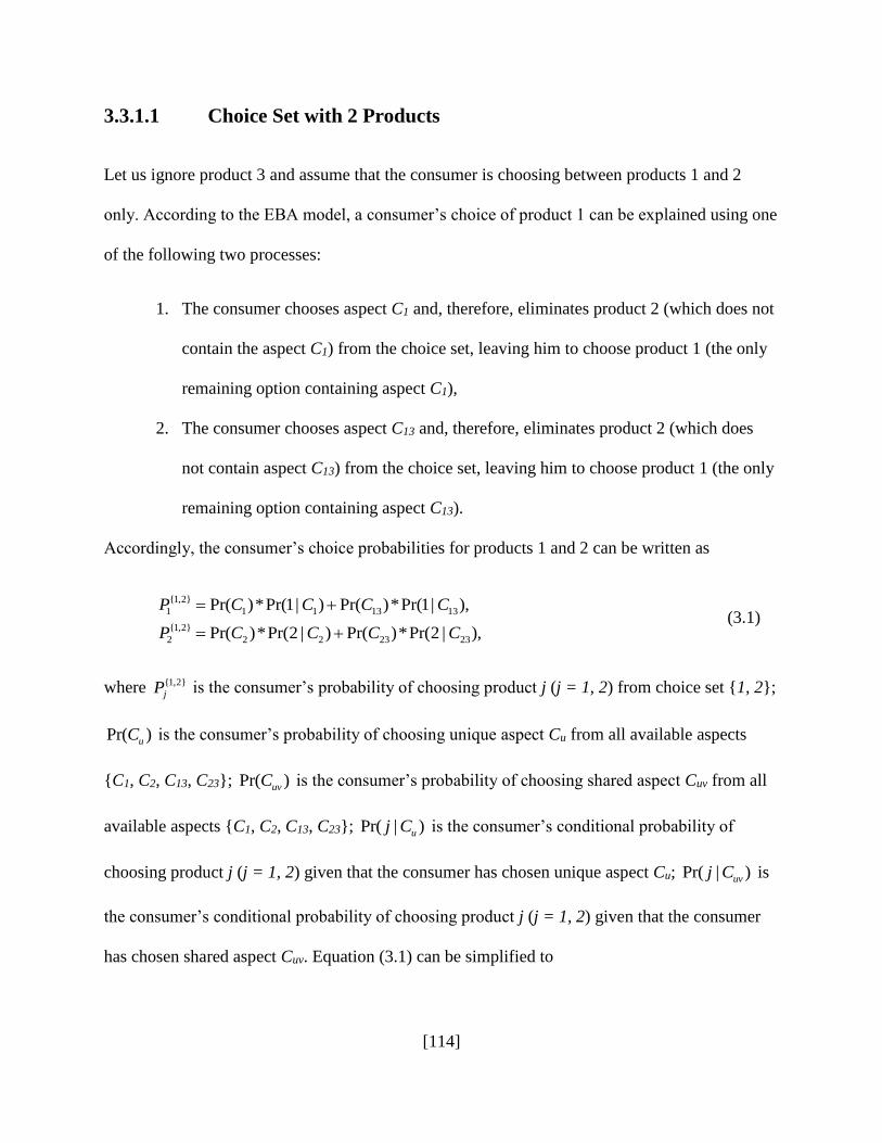
[114]

3.3.1.1 Choice Set with 2 Products

Let us ignore product 3 and assume that the consumer is choosing between products 1 and 2

only. According to the EBA model, a consumer’s choice of product 1 can be explained using one

of the following two processes:

1. The consumer chooses aspect C1 and, therefore, eliminates product 2 (which does not

contain the aspect C1) from the choice set, leaving him to choose product 1 (the only

remaining option containing aspect C1),

2. The consumer chooses aspect C13 and, therefore, eliminates product 2 (which does

not contain aspect C13) from the choice set, leaving him to choose product 1 (the only

remaining option containing aspect C13).

Accordingly, the consumer’s choice probabilities for products 1 and 2 can be written as

{1,2}

1 1 1 13 13

{1,2}

2 2 2 23 23

Pr( )*Pr(1| ) Pr( )*Pr(1| ),

Pr( )*Pr(2 | ) Pr( )*Pr(2 | ),

P C C C C

P C C C C

(3.1)

where {1,2}

jP is the consumer’s probability of choosing product j (j = 1, 2) from choice set {1, 2};

Pr( )uC is the consumer’s probability of choosing unique aspect Cu from all available aspects

{C1, C2, C13, C23}; Pr( )uvC is the consumer’s probability of choosing shared aspect Cuv from all

available aspects {C1, C2, C13, C23}; Pr( | )uj C is the consumer’s conditional probability of

choosing product j (j = 1, 2) given that the consumer has chosen unique aspect Cu; Pr( | )uvj C is

the consumer’s conditional probability of choosing product j (j = 1, 2) given that the consumer

has chosen shared aspect Cuv. Equation (3.1) can be simplified to

[115]

{1,2}

1 1 13

{1,2}

2 2 23

Pr( ) Pr( ),

Pr( ) Pr( ),

P C C

P C C

(3.2)

because each conditional probability (representing the consumer’s probability of choosing a

brand from a singleton choice set containing that brand only) on the right hand side of equation

(3.1) is 1. The aspect choice probabilities are obtained by scaling the aspect parameters to yield

{1,2} 1311

1 2 13 23 1 2 13 23

{1,2} 2322

1 2 13 23 1 2 13 23

,

,

CCP

C C C C C C C C

CCP

C C C C C C C C

(3.3)

which, in turn, reduces to

{1,2} 1 131

1 2 13 23

{1,2} 2 232

1 2 13 23

,

,

C CP

C C C C

C CP

C C C C

(3.4)

which represent the consumer’s EBA choice probabilities for the choice set {1, 2}. Similarly, the

consumer’s EBA choice probabilities for the choice set {1, 3) are

{1,3} 1 121

1 3 12 23

{1,3} 3 233

1 3 12 23

,

,

C CP

C C C C

C CP

C C C C

(3.5)

and the consumer’s choice probabilities for the choice set {2, 3} are

{2,3} 2 122

2 3 12 13

{2,3} 3 133

2 3 12 13

,

.

C CP

C C C C

C CP

C C C C

(3.6)

[116]

To summarize, equations (4) - (6) represent the consumer’s EBA choice probabilities for choice

sets with 2 products. Notice that in a choice set, aspects that are shared by all products do not

play a role in the choice probabilities. For example, {1,2}

jP is not a function of C12. Let us next

consider the full choice set with 3 products.

3.3.1.2 Choice Set with 3 Products

Now the consumer is choosing between products 1, 2 and 3. According to the EBA model, a

consumer’s choice of product 1 can be explained using one of the following two processes:

1. The consumer chooses aspect C1 and, therefore, eliminates products 2 and 3 (neither

of which contains aspect C1) from the choice set, leaving him to choose product 1,

2. The consumer chooses aspect C12 and, therefore, eliminates product 3 (which does

not contain aspect C12) from the choice set, leaving him to choose product 1 from the

choice set {1, 2},

3. The consumer chooses aspect C13 and, therefore, eliminates product 2 from the choice

set, leaving him to choose product 1 from the choice set {1, 3}.

Accordingly, the consumer’s choice probabilities for products 1, 2 and 3 can be written as

{1,2,3} {1,2} {1,3}

1 1 12 1 13 1

{1,2,3} {1,2} {2,3}

2 2 12 2 23 2

{1,2,3} {1,3} {2,3}

3 3 13 3 23 3

Pr( ) Pr( )* Pr( )* ,

Pr( ) Pr( )* Pr( )* ,

Pr( ) Pr( )* Pr( )* ,

P C C P C P

P C C P C P

P C C P C P

(3.7)

which reduces to

[117]

{1,2} {1,3}{1,2,3} 1 12 1 13 1

1

1 2 3 12 13 23

{1,2} {2,3}{1,2,3} 2 12 2 23 2

2

1 2 3 12 13 23

{1,3} {2,3}{1,2,3} 3 13 3 23 3

3

1 2 3 12 13 23

* *,

* *,

* *,

C C P C PP

C C C C C C

C C P C PP

C C C C C C

C C P C PP

C C C C C C

(3.8)

where the probabilities {1,2}

1P , {1,2}

2P , {1,3}

1P , {1,3}

3P , {2,3}

2P , {2,3}

3P are as given in equations (3.4) –

(3.6). Equation (3.8) represents the consumer’s EBA choice probabilities for the choice set {1, 2,

3}.

3.3.2 Step 2: Random Utility Formulation (RUF) of Tversky’s (1972) EBA

Model

Consider a consumer whose indirect utilities for the products in choice set {1, 2} are

{1,2}

1 1 13 1

{1,2}

2 2 23 2

ln ,

ln ,

U C C

U C C

(3.9)

where C1, C2, C13 and C23 represent product aspects as explained earlier, ε1 and ε2 represent the

stochastic components of the consumer’s utilities for the 2 products. Suppose we assume ε1 and

ε2 to be distributed iid Gumbel with location parameter 0 and scale parameter 1, then the

consumer’s choice probabilities for the 2 products are given by equation (3.4). Similarly, if the

consumer’s indirect utilities for the products in choice set {1, 3} are

{1,3}

1 1 12 1

{1,3}

3 3 23 3

ln ,

ln ,

U C C

U C C

(3.10)

[118]

then the consumer’s choice probabilities for the 2 products are given by equation (3.5).

Similarly, if the consumer’s indirect utilities for the products in choice set {1, 3} are

{2,3}

2 2 12 2

{2,3}

3 3 13 3

ln ,

ln ,

U C C

U C C

(3.11)

then the consumer’s choice probabilities for the 2 products are given by equation (3.6). In other

words, equations (3.9) – (3.11) represent random utility formulations of Tversky’s EBA choice

probabilities (3.4) – (3.6). The deterministic component of each random utility is a composite of

all aspects that render the product to be uniquely different from the other product. Extending this

argument, if the consumer’s indirect utilities for the products in the choice set are {1, 2, 3} are

{1,2,3} {1,2} {1,3}

1 1 12 1 13 1 1

{1,2,3} {1,2} {2,3}

2 2 12 2 23 2 2

{1,2,3} {1,3} {2,3}

3 3 13 3 23 3 3

ln * * ,

ln * * ,

ln * * ,

U C C P C P

U C C P C P

U C C P C P

(3.12)

then the consumer’s choice probabilities for the 3 products are given by equation (3.8). Again,

the deterministic component of each random utility represents what is unique about the product

when compared to the other 2 products in the choice set. For example, consider the utility

equation for product 1. There are 3 terms within parentheses. The first term, C1, directly

represents what is unique to product 1. The second term has 2 components, C12 and {1,2}

1P . While

the first component represents what is unique to both products 1 and 2 when compared to

product 3, the second component represents what is unique to product 1 when compared to

product 2 (as explained under equation (3.11)), therefore, the two multiplicative components

collectively represent what is unique to product 1. Similar arguments apply for the third term.

[119]

3.3.3 Step 3: Extending the RUF of Tversky’s (1972) EBA Model to Handle

Marketing Variables

Since we have established a random utility formulation that is mathematically equivalent to

Tversky’s EBA model, extending the model to incorporate the effects of marketing variables (or,

more generally, time-varying covariates) is straightforwardly achieved as follows.

{1,2,3} {1,2} {1,3}

1 1 1 12 1 13 1 1

{1,2,3} {1,2} {2,3}

2 2 2 12 2 23 2 2

{1,2,3} {1,3} {2,3}

3 3 3 13 3 23 3 3

ln * * ,

ln * * ,

ln * * ,

U X C C P C P

U X C C P C P

U X C C P C P

(3.13)

where X1, X2 and X3 represent 3-dimensional row vectors representing the price, display and

feature that are associated with the product, and is the corresponding 3-dimensional column

vector of parameters. Similarly, we get

{1,2}

1 1 1 13 1

{1,2}

2 2 2 23 2

ln ,

ln ,

U X C C

U X C C

(3.14)

and

{1,3}

1 1 1 12 1

{1,3}

3 3 3 23 3

ln ,

ln ,

U X C C

U X C C

(3.15)

and

{2,3}

2 2 2 12 2

{2,3}

3 3 3 13 3

ln ,

ln ,

U X C C

U X C C

(3.16)

where all the error terms are iid Gumbel (0, 1).

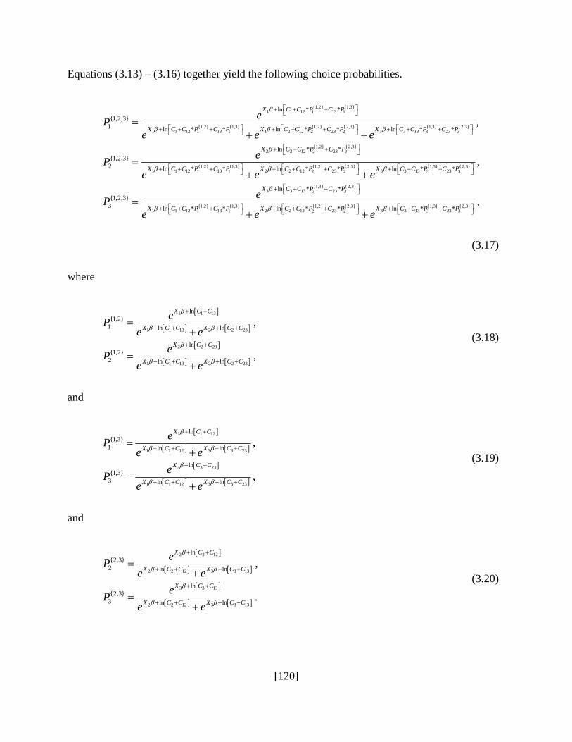
[120]

Equations (3.13) – (3.16) together yield the following choice probabilities.

{1,2} {1,3}1 1 12 131 1

{1,2} {1,3} {1,2} {2,3} {1,3} {2,3}1 1 12 13 1 2 12 23 3 3 13 231 1 2 2 3 3

{1,2} {2 2 12 232 2

ln * *

{1,2,3}

1 ln * * ln * * ln * *

ln * *

{1,2,3}

2

,

X C C P C P

X C C P C P X C C P C P X C C P C P

X C C P C P

eP

e e e

eP

2,3}

{1,2} {1,3} {1,2} {2,3} {1,3} {2,3}1 1 12 13 2 2 12 23 3 3 13 231 1 2 2 3 3

{1,3} {2,3}3 3 13 233 3

{1,2} {1,1 1 12 131 1

ln * * ln * * ln * *

ln * *

{1,2,3}

3 ln * *

,X C C P C P X C C P C P X C C P C P

X C C P C P

X C C P C P

e e e

eP

e

3} {1,2} {2,3} {1,3} {2,3}

2 2 12 23 3 3 13 232 2 3 3ln * * ln * *,

X C C P C P X C C P C Pe e

(3.17)

where

1 1 13

1 1 13 2 2 23

2 2 23

1 1 13 2 2 23

ln

{1,2}

1 ln ln

ln

{1,2}

2 ln ln

,

,

X C C

X C C X C C

X C C

X C C X C C

eP

e e

eP

e e

(3.18)

and

1 1 12

3 3 231 1 12

3 3 23

3 3 231 1 12

ln

{1,3}

1 lnln

ln

{1,3}

3 lnln

,

,

X C C

X C CX C C

X C C

X C CX C C

eP

e e

eP

e e

(3.19)

and

2 2 12

3 3 132 2 12

3 3 13

3 3 132 2 12

ln

{2,3}

2 lnln

ln

{2,3}

3 lnln

,

.

X C C

X C CX C C

X C C

X C CX C C

eP

e e

eP

e e

(3.20)

[121]

This completes the exposition of our proposed model. Equations (3.17) – (3.20) collectively

represent our proposed EBA demand model for differentiated products. When = 0, our

model reduces to Tversky’s (1972) EBA model. When all shared aspects, Cuv, are 0, our model

reduces to the familiar logit model.

The key theoretical difference between the indirect utility formulation of the EBA, as

discussed here, and the indirect utility formulation that is typically invoked in random utility

models (such as the logit, probit etc.) is two-fold: (1) the indirect utility yielded by a brand to the

consumer under our EBA formulation is choice-set specific, as represented by the superscripts on

the left-hand side of equations (3.13) - (3.16), while the indirect utility is not choice-set specific

in existing random utility models; this property of the EBA can be taken to be a manifestation of

what behavioral researchers label context effects in demand, where consumers’ preferences for

brands depend on the choice context (in our case, the choice set); (2) the presence of lower-order

choice probabilities (e.g., {1,2}

1P ) within the consumer’s indirect utility function for brands in

higher-choice choice sets (e.g., {1,2,3}

1U ) appears atheoretical; the reason is that the indirect utility

function in equation (3.13) must be interpreted as a reduced-form solution to a deeper utility-

theoretic specification of the impact of brands’ aspects on consumer’s direct utilities for brands,

much like the use of lagged choice indicators or brand loyalty variables in random utility models

to represent structural state dependence (Guadagni and Little 1983).

In the absence of, or indifference toward, a random utility formulation, one could view

the EBA and, therefore, our proposed extension of the EBA, as a probabilistic model of

consumer choice. In that case, the consumer’s choice probability for a brand is directly specified

by overlaying multiplicative terms, which represent the exponentiated attractiveness of brands in

[122]

terms of their marketing mix, in the numerators and denominators of the original EBA choice

probabilities. This is illustrated below for the choice set (1, 2).

1

1 2

2

1 2

1 13{1,2}

1

1 13 2 23

2 23{1,2}

2

1 13 2 23

,

,

X

X X

X

X X

C C eP

C C e C C e

C C eP

C C e C C e

(3.21)

which is mathematically equivalent to equation (3.18). Whether one directly works with the

choice probabilities, or additionally derives them from random utility primitives (as we do), is a

matter of personal research taste. The modeling flexibility of the EBA accrues regardless of this

taste.

3.4 Estimation of Our Proposed Model Using Aggregate

Scanner Data

Before we discuss estimation, let us first explain what is observed in aggregate scanner data. In

any given day, we observe an outcome vector yt = (y1t y2t … yJt)’, where each element yjt

represents the unit sales for brand j during day t. Further, during each day t, we observe the price

(Pjt), display (Djt), and feature (Fjt) covariates associated with each brand j. We assume the

market size, Mt, to be equal to the total number of transactions observed in the store during day t.

We then assume that each unit of each brand sold in a given day t is to a different household.

Each household, in turn, is assumed to choose among J+1 options (J brands plus the outside

good) in the category. Demand for the outside good, y0t, is imputed in the usual way by

subtracting the summed sales across all J brands from the market size. These assumptions are

[123]

typically invoked in market share models (e.g., Sudhir 2001, Chintagunta 2001, Mantrala et al.

2006) since neither individual household choices nor purchase incidences / quantities are

explicitly observed in aggregate scanner data.

Let Pjt denote the choice probability, under our proposed model, for a household for

brand j in day t. These are given by equation (3.17), suitably extended to the case of J brands

(see Batsell et al. (2003) for a canonical algebraic representation of Tversky’s (1972) original

EBA model for the J-brand case, but without time-varying covariates, within which one could

incorporate marketing variables as in equation (3.17)). In these choice probabilities, each brand’s

intercept term will involve not only the brand’s unique aspect (Cj) but also all shared aspects that

are contained in that brand (i.e., Cjk’s, Cjkl’s etc.). Further the J choice probabilities will each

contain lower-order, i.e., (J-1), (J-2) etc., choice probabilities on the right-hand side, as in

equation (3.17). The following likelihood function is maximized to estimate model parameters.

1 0

,jt

T Jy

jt

t j

L P

(3.22)

where T is the number of days in the aggregate scanner data. For a recent application of

Tversky’s (1972) original EBA model to discrete choice experimental data, see Gilbride and

Allenby (2006).

To obtain model parsimony and, therefore, a clear behavioral explanation of consumer

choice behavior, the estimation of an EBA model should result in a compact number of shared

aspects that can be easily interpreted given what is known about the products, which additionally

renders the model to be managerially actionable. For this purpose, although we begin with the

estimation of all possible aspects (30 in our 5-product case), we sequentially remove

[124]

insignificant aspects from the model. The aspects are removed one-by-one as long as the BIC

improves, much like segments are added in the discrete mixed logit as long as the BIC improves.

Once the removal of an aspect fails to improve the BIC, we then try the removal of other aspects

to see if a better fit can still be established. With regard to which aspect to remove, we use aspect

significance. While it may take some time to calculate aspect significance, aspect magnitude is

highly correlated with significance and can also be used as the determinant of removal (initially,

many aspects will be very close to zero). We have used both removal rules with nearly identical

results.

3.4.1 Identification of Shared Aspects

It is useful to explain what aspect of aggregate scanner data permit the estimation of the shared

aspect parameters, especially since the constitution of the available choice set of brands at a store

does not vary from day to day (which, if it were not the case, would allow one to exploit the

entries and exits of one or more brands, and the consequent impacts on the demands of the

remaining brands, to estimate the shared aspects). When the relative prices, displays and features

of the J brands change from one day to another, the unit sales of the brands change as a

consequence. This variation enables the estimation of shared aspects. For example, if the

decrease in price of brand i decreases the demand of brand j disproportionately more than it

decreases the demand of brand k (beyond what is implied by their current relative market shares),

then it would serve as the source of identification of a shared aspect between brands i and j. If it

decreases the demand of both brands j and l, then it would serve as the source of identification of

a shared aspect between brands i, j and l. On the other hand, if demand of brand i is relatively

immune to the price cuts of any of the other brands, then it would serve to identify the unique

[125]

aspect of brand i. It is the incorporation of these time-varying covariates (such as price, display

and feature) that allows for identification the EBA model on scanner data. Previously, the EBA

model required either survey data with varying choice sets or stock-out data in order to provide

variation in Pr( | )uvj C and, therefore, permit the identification of the shared aspects. In fact, it is

the presence of shared aspects in our proposed demand model that makes it immune to the

Invariant Proportion of Substitution (IPS) restriction of the mixed logit, which was first pointed

out by Steenburgh (2008). In our proposed demand model, attribute similarity among products

plays a central role in explaining shifts in market share among brands in response to relative

changes in the marketing mix. This feature is critical while employing a demand model for

differentiated products.

3.4.2 Comparison Models

We estimate the mixed logit and probit as comparison models. The mixed logit is operationalized

as follows: in equation (3.15), we set all shared aspects, Cuv, to 0, which reduces our model to the

logit; we then assume that the intercept terms of the logit, i.e., the logarithms of the unique

aspects of the products, follow a random distribution. We make two alternative assumptions

about this random distribution: (1) semi-parametric, with discrete support points (“discrete mixed

logit”), (2) multivariate normal with a general covariance structure (“continuous mixed logit”).

The probit is operationalized as follows: in equation (3.15), we set all shared aspects, Cuv,

to 0, plus assume that the error terms are distributed normal (instead of Gumbel) with a general

covariance structure. We do not estimate a nested logit for the reason discussed in the

introduction section, i.e., it requires all possible tree structures to be explicitly allowed for and

[126]

estimated on the data which is computationally impractical, which is why it has been ignored in

the literature on market share models.

An alternative formulation of price within Tversky’s (1972) EBA model has been

proposed by Rotondo (1986). However, that model requires the a priori ad-hoc specification of,

as well the estimation of, a large number of price cut-off parameters. Further, incorporating

additional time-varying covariates beyond price (such as display and feature) vastly increases the

dimensionality of the parameter space. Also, the model is not based on random utility primitives.

Therefore, appropriately specifying and estimating a suitable version of the Rotondo (1986)

model for our aggregate scanner data, for comparison, is beyond the scope of our analyses.

Fader and McAlister (1990) propose a market share model that can handle promotional

variables. However, much like the nested logit, their model also requires a priori specification,

rather than the endogenous determination, of a decision tree. Gilbride and Allenby (2006), as

noted earlier, only estimate a traditional EBA model (without marketing variables) using

experimental choices, and not market shares.

3.5 Numerical Illustrations of Similarity and Dominance

Effects in Demand

First, we illustrate, using two numerical examples, the relative ability of the EBA to handle

similarity and dominance effects in demand when compared to the nested logit and mixed logit.

Second, we illustrate, using a third numerical example, the difference between our proposed

demand model and the logit in explaining demand data with marketing variables, and derive the

[127]

implied differences in price elasticities between the two models. Third, we illustrate, using a

fourth numerical example, the probit’s inability to handle similarities among more than two

brands, unlike the EBA. Fourth, we simulate demand data, with marketing variables included,

using our proposed demand model, and then study the consequences of estimating the mixed

logit and the probit on the simulated data.

3.5.1 EBA versus Nested Logit, Mixed Logit and Logit

Consider the following set of 3 western classical symphonies: (1) Mozart’s 5th Symphony (M),

(2) Beethoven’s 5th Symphony (B1) and (3) Beethoven’s 7th Symphony (B2). Suppose we run a

discrete choice experiment in which consumers in a lab are presented multiple choice sets and

asked to choose one symphony within each choice set, where the choice sets are constructed

using all possible subsets of the above 3 symphonies (with at least two alternatives in a choice

set). The choice sets, along with the observed choice shares are given below in Table 3.1.

Table 3.1: Choice Shares Displaying Similarity Effects in Demand (Numerical Example 1)

(Within parentheses are the choice shares fitted by the logit)

______________________________________________________________________________

Choice Set Observed Choice Share

Composition M B1 B2

(M, B1) 0.58 (0.64) 0.42 (0.36) na

(M, B2) 0.58 (0.64) na 0.42 (0.36)

(B1, B2) na 0.50 (0.50) 0.50 (0.50)

(M, B1, B2) 0.58 (0.47) 0.21 (0.27) 0.21 (0.27)

[128]

As can be observed above, the logit, which allows for only the unique aspect parameters

of the three products (whose maximum likelihood estimates in this case are 0.47, 0.27 and 0.27),

cannot fit the observed choice shares. It overestimates the choice share of M in (M, B1) and

underestimates its share in (M, B1, B2). It is easy to show that a suitably specified nested logit

(which groups B1 and B2 within one nest, and M within another), as well as a mixed logit, and

the EBA can perfectly fit the above shares. However, the EBA and nested logit do so more

parsimoniously (using 3 effective parameters, CMB1, CMB2, CB1B2, with CM normalized) than the

mixed logit (which uses 5 effective parameters). In addition, given that researchers typically use

penalized fit criteria, such as the BIC, to identify the optimal number of support points for a

discrete mixed logit, it is often the case that one stops adding support points sooner than is

warranted to fully relax the similarity and dominance restrictions in the data (in fact, we find this

to be the case in our numerical simulations where we accept the one support solution based on

BIC when, in fact, the two-support solution is required to handle the simulated similarity and

dominance patterns). Therefore, even when the mixed logit is capable of successfully handling

the similarity and dominance patterns in the data, identifying the appropriate mixed logit is often

stymied in the estimation.

Now consider the case of dominance. Suppose that the choice sets, along with the

observed choice shares are as given below in Table 3.2. Again, the logit, (whose unique aspects

in this case are 0.43, 0.48 and 0.09), cannot fit the observed choice shares. It underestimates the

choice share of M in (M, B1) and in (M, B1, B2) and greatly overestimates it in (M, B2).

Interestingly, even the best-fitting, among all possible tree structures, nested logit does almost as

badly as the logit, which shows that the nested logit cannot handle dominance effects. The mixed

logit and the EBA can perfectly fit the above shares. However, the EBA does so more

[129]

parsimoniously (using 2 effective parameters, CM (normalized), CMB1, CB1B2) than the mixed logit

(which uses 5 effective parameters).

Table 3.2: Choice Shares Displaying Dominance Effects in Demand (Numerical Example 2)

(Within parentheses are the choice shares fitted by the logit, nested logit)

______________________________________________________________________________


Composition M B1 B2

(M, B1) 0.58 (0.48, 0.38) 0.42 (0.52, 0.62) na

(M, B2) 0.58 (0.83, 0.78) na 0.42 (0.17, 0.22)

(B1, B2) na 1 (0.84, 0.86) 0 (0.16, 0.14)

(M, B1, B2) 0.58 (0.43, 0.58) 0.42 (0.48, 0.36) 0 (0.09, 0.36)

The above numerical examples show that the mixed logit cannot handle similarity and

dominance effects in general. While the mixed logit can accommodate both similarity and

dominance effects in the simple case of 3 alternatives, identifying the appropriate mixed logit

using fit criteria, such as BIC, leads to an under-specified model that does not adequately handle

similarity and dominance effects. However, the empirically identified EBA always handles

similarity and dominance effects in the data, and does so with far fewer parameters than the

mixed logit and, thus, has greater predictive efficiency. Further, we find that when we impose

only a moderate level of dominance (rather than the extreme dominance in Table 3.2) in the data,

we find that the EBA becomes even more parsimonious compared to the mixed logit in that it

requires fewer effective parameters to fit the data (results are available from the authors). As

noted earlier, the “mixture” in the mixed logit also has no behavioral interpretation at the

individual-level since it represents across-consumer heterogeneity. However, the EBA is

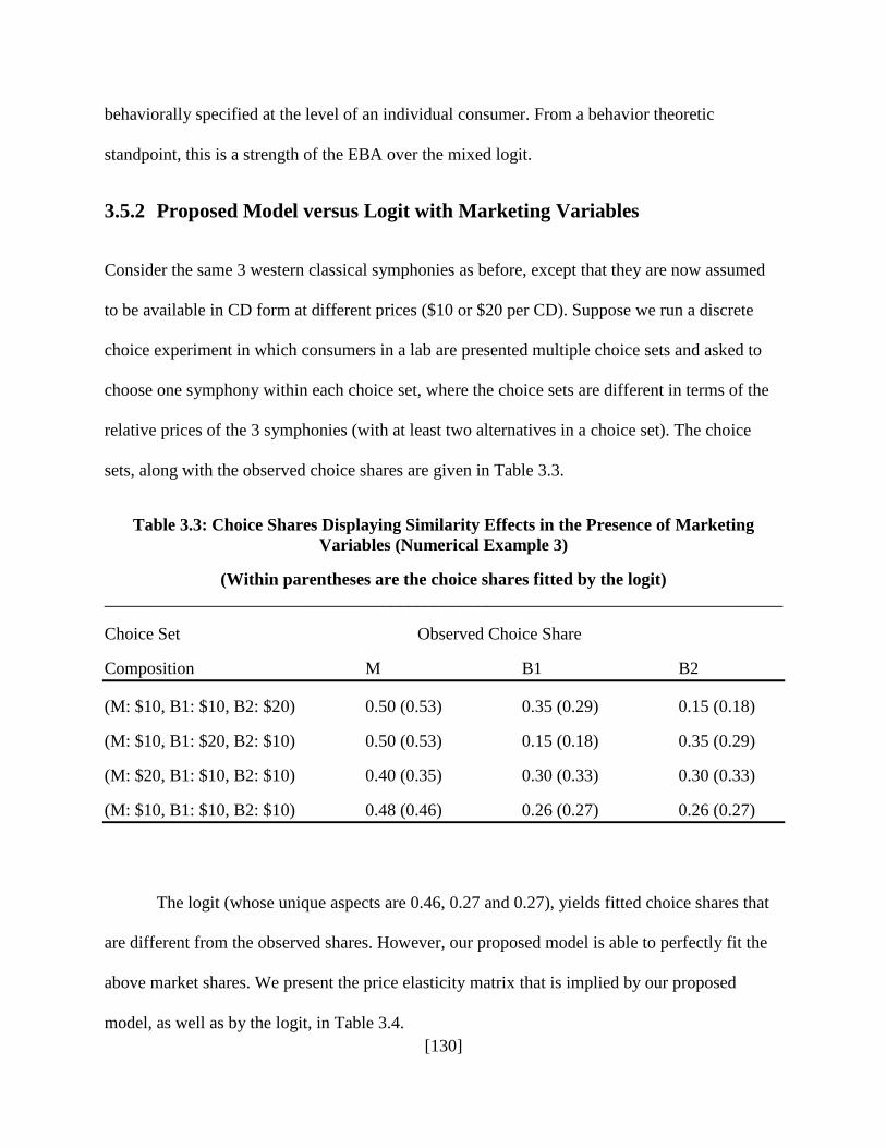
[130]

behaviorally specified at the level of an individual consumer. From a behavior theoretic

standpoint, this is a strength of the EBA over the mixed logit.

3.5.2 Proposed Model versus Logit with Marketing Variables

Consider the same 3 western classical symphonies as before, except that they are now assumed

to be available in CD form at different prices ($10 or $20 per CD). Suppose we run a discrete

choice experiment in which consumers in a lab are presented multiple choice sets and asked to

choose one symphony within each choice set, where the choice sets are different in terms of the

relative prices of the 3 symphonies (with at least two alternatives in a choice set). The choice

sets, along with the observed choice shares are given in Table 3.3.

Table 3.3: Choice Shares Displaying Similarity Effects in the Presence of Marketing

Variables (Numerical Example 3)

(Within parentheses are the choice shares fitted by the logit)

______________________________________________________________________________


Composition M B1 B2

(M: $10, B1: $10, B2: $20) 0.50 (0.53) 0.35 (0.29) 0.15 (0.18)

(M: $10, B1: $20, B2: $10) 0.50 (0.53) 0.15 (0.18) 0.35 (0.29)

(M: $20, B1: $10, B2: $10) 0.40 (0.35) 0.30 (0.33) 0.30 (0.33)

(M: $10, B1: $10, B2: $10) 0.48 (0.46) 0.26 (0.27) 0.26 (0.27)

The logit (whose unique aspects are 0.46, 0.27 and 0.27), yields fitted choice shares that

are different from the observed shares. However, our proposed model is able to perfectly fit the

above market shares. We present the price elasticity matrix that is implied by our proposed

model, as well as by the logit, in Table 3.4.

[131]

Table 3.4: Price Elasticity Matrix Implied by Proposed Model in the Presence of Marketing

Variables (Numerical Example 3)

(Within parentheses are the price elasticities implied by the logit)

______________________________________________________________________________

% Change in demand of column brand for % change in price of row brand

M B1 B2

M -0.21 (-0.27) 0.19 (0.24) 0.19 (0.24)

B1 0.10 (0.14) -0.49 (-0.38) 0.30 (0.14)

B2 0.10 (0.14) 0.30 (0.14) -0.49 (-0.38)

___________________________________________________________________________

The cross-elasticities in the third row of Table 3.4 are seriously mis-estimated by the logit

when compared to our proposed model. For example, the cross-elasticity of B1 demand with

respect to B2 price is 0.30 according to our proposed model, but only 0.14 according to the logit.

To the extent that these price elasticities serve as inputs to figuring out optimal retail prices of

the 3 brands, significant distortions in the estimated price elasticities will lead to seriously sub-

optimal prices and, therefore, lowered retail profits. We explicitly investigate these issues in

section 5.

3.5.3 EBA versus Probit

To illustrate the probit’s inability to handle similarities among three (or more) brands, consider

the following set of four soft drink brands: (1) Sprite (S), (2) Coke (C), (3) Pepsi (P) and (4) RC

Cola (RC). Suppose we run a discrete choice experiment in which consumers in a lab are

presented multiple choice sets and asked to choose one soft drink within each choice set, where

the choice sets are constructed using all possible subsets of the above 4 options (with at least two

[132]

alternatives in a choice set). Suppose that some of these consumers prefer non-cola (i.e., S),

while others prefer cola (i.e., C, P, RC). Suppose further that all of these consumers strictly

prefer C or P over RC, but are indifferent between C and P. The probit cannot fully represent this

situation. While the probit can successfully represent the preference for cola using all possible

pair-wise correlations among C, P and RC, it cannot simultaneously capture the dominance of C

and P over RC. On the other hand, the EBA can. The choice sets, along with the observed

choice shares and the predicted choice shares yielded by the probit are given in Table 3.5. The

probit consistently under-predicts the choice share of S and especially struggles when predicting

Table 3.5: Choice Shares Displaying Dominance Effects in Demand (Numerical Example 4)

(Within parentheses are the choice shares fitted by the probit)

______________________________________________________________________________


Composition S C P RC

(S, C) 0.6 (0.56) 0.4 (0.45) na na

(S, P) 0.6 (0.54) na 0.4 (0.46) na

(S, RC) 0.6 (0.83) na na 0.4 (0.17)

(C, P) na 0.5 (0.48) 0.5 (0.52) na

(C, RC) na 1.0 (0.99) na 0.0 (0.01)

(P, RC) na na 1.0 (0.99) 0.0 (0.01)

(S, C, P) 0.6 (0.55) 0.2 (0.25) 0.2 (0.20) na

(S, C, RC) 0.6 (0.53) 0.4 (0.45) na 0.0 (0.02)

(S, P, RC) 0.6 (0.56) na 0.4 (0.43) 0.0 (0.01)

(C, P, RC) na 0.5 (0.51) 0.5 (0.49) 0.0 (0.00)

(S, C, P, RC) 0.6 (0.55) 0.2 (0.22) 0.2 (0.22) 0.0 (0.01)

[133]

choice shares in the choice set containing S and RC. The EBA perfectly predicts the choice

shares in all choice sets.

3.5.4 Proposed Model versus Discrete Mixed Logit, Continuous Mixed Logit

and Probit

We simulate brands’ market shares in a fictional 5-brand category over 10,000 days using our

proposed demand model and assuming the following demand parameters: C1 = 3.9, C2 = 4, C3 =

3, C45 = 5, C124 = 1, C235 = 3, P = -1.5, D = 0.35, F = 0.25. We draw the prices of the 5

brands independently from Uniform (0, 6) distributions and the displays and features of the 5

brands independently from Uniform (0, 1) distributions. We estimate our proposed demand

model, discrete mixed logit, continuous mixed logit and probit using the first 9000 days of the

simulated data (our proposed model perfectly recovers the assumed parameters). We predict

holdout outcomes in the last 1000 days. The results of the comparison are in Table 3.6 below.

Table 3.6: Performance Comparison of Models on Simulated Data

(Note: The discrete mixed logit is based on a 7-support distribution)

______________________________________________________________________________

Performance Proposed Discrete Continuous Probit

Criterion Model Mixed Logit Mixed Logit

______________________________________________________________________________

In-sample LL -6221 -6269 -6302 -6721

In-sample BIC 12516 13040 12740 13596

Holdout LL -694 -699 -703 -750

Holdout MSE 4.7E-13 0.0012 0.0014 0.0099

Holdout MAD 1.6E-7 0.0241 0.0294 0.0786

[134]

The EBA model dramatically outperforms the comparison models in terms of aggregate

predictive metrics, i.e., Mean Squared Error (MSE) and Mean Absolute Deviation (MAD),

which are of focal interest when making market share predictions. This happens despite our

using a fully saturated discrete mixed logit with 7 support points. Even such a fully saturated

discrete logit cannot explain the simulated data while the EBA can. In practice, since researchers

use the “best-fitting” (in terms of criteria such as BIC) discrete mixed logit, which will have far

fewer support points than 7, for prediction purposes, the difference between the EBA and such a

discrete mixed logit will be even more striking in practice. Next we compare the models using

empirical data.

3.6 Empirical Results

We employ scanner data from a single store in a midwestern market tracking the choices of

panelists in 9 different product categories (which have been identified as representing the typical

shopping basket of a US household, see Bell and Lattin 1998) – bacon, butter, coffee, soda,

crackers, detergent, hot dogs, ice cream, tissue -- over a 104-week period (1993-1995). We use

the aggregate sales across all panelists for analysis purposes. We partition the aggregate sales

data for each category into two subsets: estimation sample (91 weeks of data), and holdout

sample (13 weeks). The top 4 brands in each category are aggregates of all SKUs under the same

brand name, and are treated as the 4 focal brands. They account for the following cumulative

shares in the 9 listed categories: 82%, 58%, 66%, 48%, 43%, 54%, 52%, 59%, 66%,

respectively. We lump the remaining brands in to an alternative called “Other” which is also

taken to represent the outside good for our pricing simulations (discussed in the next section).

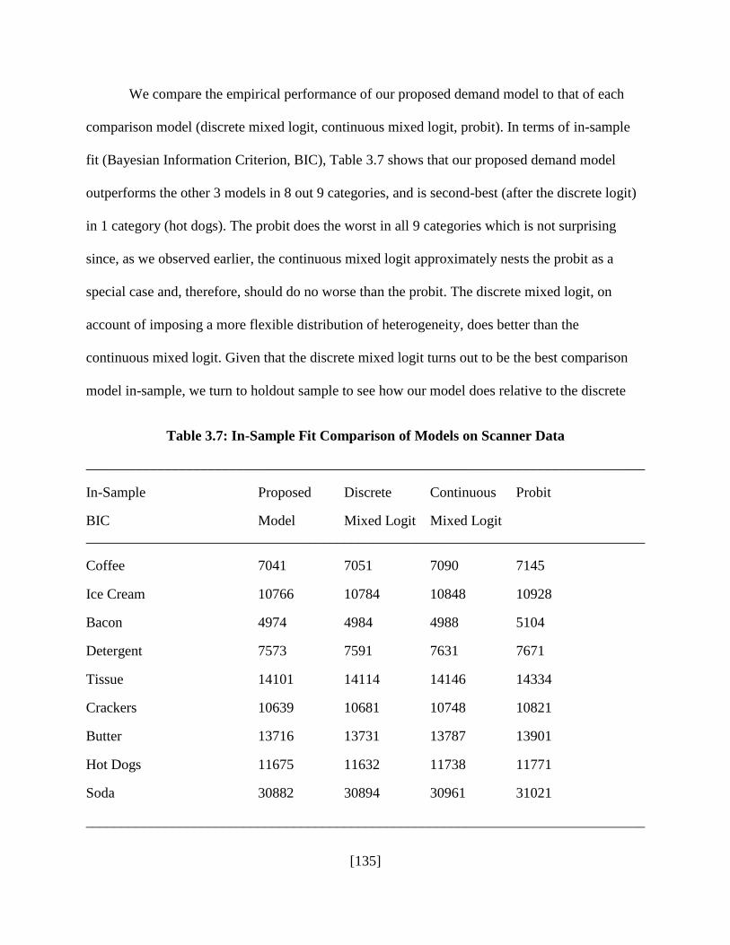
[135]

We compare the empirical performance of our proposed demand model to that of each

comparison model (discrete mixed logit, continuous mixed logit, probit). In terms of in-sample

fit (Bayesian Information Criterion, BIC), Table 3.7 shows that our proposed demand model

outperforms the other 3 models in 8 out 9 categories, and is second-best (after the discrete logit)

in 1 category (hot dogs). The probit does the worst in all 9 categories which is not surprising

since, as we observed earlier, the continuous mixed logit approximately nests the probit as a

special case and, therefore, should do no worse than the probit. The discrete mixed logit, on

account of imposing a more flexible distribution of heterogeneity, does better than the

continuous mixed logit. Given that the discrete mixed logit turns out to be the best comparison

model in-sample, we turn to holdout sample to see how our model does relative to the discrete

Table 3.7: In-Sample Fit Comparison of Models on Scanner Data

______________________________________________________________________________

In-Sample Proposed Discrete Continuous Probit

BIC Model Mixed Logit Mixed Logit

______________________________________________________________________________

Coffee 7041 7051 7090 7145

Ice Cream 10766 10784 10848 10928

Bacon 4974 4984 4988 5104

Detergent 7573 7591 7631 7671

Tissue 14101 14114 14146 14334

Crackers 10639 10681 10748 10821

Butter 13716 13731 13787 13901

Hot Dogs 11675 11632 11738 11771

Soda 30882 30894 30961 31021

______________________________________________________________________________

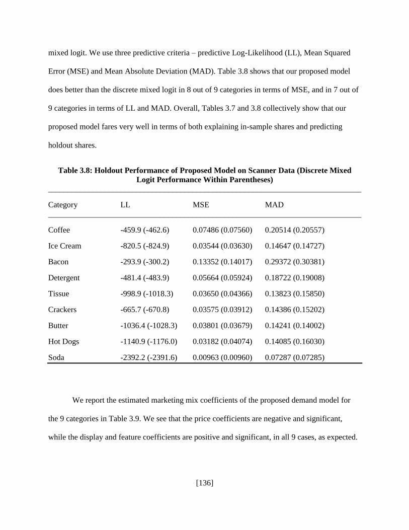
[136]

mixed logit. We use three predictive criteria – predictive Log-Likelihood (LL), Mean Squared

Error (MSE) and Mean Absolute Deviation (MAD). Table 3.8 shows that our proposed model

does better than the discrete mixed logit in 8 out of 9 categories in terms of MSE, and in 7 out of

9 categories in terms of LL and MAD. Overall, Tables 3.7 and 3.8 collectively show that our

proposed model fares very well in terms of both explaining in-sample shares and predicting

holdout shares.

Table 3.8: Holdout Performance of Proposed Model on Scanner Data (Discrete Mixed

Logit Performance Within Parentheses)

______________________________________________________________________________

Category LL MSE MAD

______________________________________________________________________________

Coffee -459.9 (-462.6) 0.07486 (0.07560) 0.20514 (0.20557)

Ice Cream -820.5 (-824.9) 0.03544 (0.03630) 0.14647 (0.14727)

Bacon -293.9 (-300.2) 0.13352 (0.14017) 0.29372 (0.30381)

Detergent -481.4 (-483.9) 0.05664 (0.05924) 0.18722 (0.19008)

Tissue -998.9 (-1018.3) 0.03650 (0.04366) 0.13823 (0.15850)

Crackers -665.7 (-670.8) 0.03575 (0.03912) 0.14386 (0.15202)

Butter -1036.4 (-1028.3) 0.03801 (0.03679) 0.14241 (0.14002)

Hot Dogs -1140.9 (-1176.0) 0.03182 (0.04074) 0.14085 (0.16030)

Soda -2392.2 (-2391.6) 0.00963 (0.00960) 0.07287 (0.07285)

We report the estimated marketing mix coefficients of the proposed demand model for

the 9 categories in Table 3.9. We see that the price coefficients are negative and significant,

while the display and feature coefficients are positive and significant, in all 9 cases, as expected.

[137]

In other words, as price of a brand decreases, its market share increases, while as display

(feature) activity on a brand increases, its market share increases, in each of the 9 categories.

The estimated aspects yielded by the proposed demand model for the 9 categories are

Table 3.9: Estimated Marketing Mix Coefficients (and standard errors)

____________________________________________________________________________

Category Price Display Feature

______________________________________________________________________________

Coffee -0.3 (0.05) 0.41 (0.06) 0.32 (0.06)

Ice Cream -2.9 (0.19) 0.63 (0.41) 0.21 (0.03)

Bacon -0.5 (0.05) 0.27 (0.05) 0.44 (0.05)

Detergent -0.5 (0.24) 0.19 (0.04) 0.39 (0.04)

Tissue -5.8 (0.78) 0.46 (0.05) 0.10 (0.04)

Crackers -0.1 (0.03) 0.26 (0.03) 0.21 (0.03)

Butter -2.2 (0.14) 0.25 (0.04) 0.20 (0.04)

Hot Dogs -0.4 (0.04) 0.31 (0.04) 0.25 (0.04)

Soda -0.6 (0.12) 0.22 (0.02) 0.07 (0.02)

reported in Table 3.10. While the total number of aspects in the 5-brand case is 30 (32 possible

subsets of 5 objects minus the null set and the universal set), the number of “effective” non-zero

aspects in a category turns out to be only either 6 or 7 (with the identities of the significant

aspects varying across categories). The remaining aspects are estimated to be 0. This is an

attractive feature of the EBA model, i.e., while it has 30 aspects in principle, which gives it great

flexibility in handling a wide range of similarity and dominance structures, only a small number

of shared aspects becomes practically necessary in order to handle the market share shifts that

are observed in aggregate scanner data. More importantly, this small number of effective aspects

[138]

is sufficient for our proposed model to outperform the mixed logit and probit, both of which have

a larger number of significantly estimated parameters (in the covariance matrices pertaining to

the marketing mix coefficients and error terms, respectively). Note that we estimate at least one

Table 3.10: Estimated Aspects

______________________________________________________________________________

Category Aspects Estimates

______________________________________________________________________________

Coffee C1 C3 C4 C25 C124 C345

1 4.4a 2.7a 1.4a 3.3a 0.76a

Ice Cream C1 C24 C25 C35 C134 C245

1 16.2a 5.5a 7.1a 6.3a 2.8a

Bacon C1 C3 C14 C123 C125 C145 C245

1 0.12a 0.17a 0.26a 0.18a 0.05c 0.53a

Detergent C1 C2 C4 C5 C123 C135 C235

1 1.9a 1.3a 0.86a 4.7a 2.2a 0.82a

Tissue C1 C2 C3 C4 C5 C1234 C1345

1 275a 32.1a 49.7a 380a 62.6a 862a

Crackers C1 C2 C45 C134 C135 C2345

1 416 155 705 924 0.35a

Butter C1 C2 C4 C5 C13 C45 C234

1 28.4a 51.4a 3.5a 12.8a 22.0a 17.0a

Hot Dogs C1 C2 C3 C5 C134 C245

1 0.34a 0.79a 1.3a 3.5a 2.8a

Soda C1 C5 C34 C235 C1234 C1245

1 0.26a 0.37a 0.81a 2.1a 0.64a

a Significant at the 1 percent level, b 5 percent, c 10 percent

[139]

triple aspect (i.e., similarity among three brands) in each category. This sheds light on our

proposed model’s ability to outperform the probit, given the probit’s limitation of only allowing

for pair-wise brand similarities.

Table 3.11 provides market share and average price, display, and feature statistics for the

5 products in the 9 categories. With this table as a reference, we will take a look at the estimated

aspects for the 3 most heavily purchased categories: soda, butter, and tissue. This exercise will

throw light on the substantive insights that can be gleaned from the EBA model.

For the soda category, we have 5 aspects apart from the normalized C1. C5 represents a

unique aspect for the non-cola private label, a product much like Sprite. To the extent that many

consumers visit the store with a strong preference for the most inexpensive, non-brand name,

option and eliminate all other options in making their choice, this aspect may reflect such

behavior. C34 is an aspect representing cola, but something other than the predominant

supermarket brand, Pepsi. C235 captures the aspect “most popular”, which, by market share,

represents Coke, Pepsi, and non-cola private label (perhaps these options enjoy the most shelf

space at the store). The aspect with the largest value is C1234, which includes all options other

than private label. This aspect reflects “brand name soda.” The final aspect is C1245, which

includes all options other than Coke, which may reflect an “anything but the most expensive”

aspect (since Coke is the most expensive product in the category).

For the butter category, apart from the normalized C1, we have 3 individual aspects, C2,

C4, C5, with the largest aspect being recovered for Land O'Lakes butter. In this category, Land

O'Lakes is the only branded product for true butter. Imperial and Shedds both specialize in non-

butter margarine and vegetable oil spreads. If a consumer wants real butter, they are likely to

[140]

choose Land O' Lakes, and its unique aspect reflects such behavior. C13 represents smaller

brands and the private label, which may reflect a “non-major brand name, but real butter” aspect.

C45 may reflect a “standard for a type of product” aspect since Land O’Lakes is the standard

brand of butter, while Shedds is the standard brand of margarine. The other brand name,

Imperial, typically offers healthier alternatives including vegetable oil and cholesterol-free

spreads. C234 includes the most expensive and most popular options.

The tissue category provides an interesting contrast to the soda category. In tissue, all 5

products have a unique aspect. Further, there are 2 "everything but" aspects. C1234 represents an

“anything but the most expensive” aspect, since it includes all products except Scott, which is

significantly more expensive than the other options. C1345 is the largest aspect in the category and

represents the "not private label" aspect. This represents a preference for a major branded

product.

The above discussion throws light on the kind of substantive insights that can be gleaned

from our proposed EBA demand model. Such rich substantive insights cannot be obtained using

the estimated covariance parameters of the mixed logit or probit. Therefore, in addition to better

explaining and predicting market shares, the EBA has superior substantive value than the mixed

logit and probit models.

Next, we derive the implications of our proposed model for retailer pricing, and compare

the resulting optimal retail prices and, more importantly, retail profits, to those yielded by the

best comparison model, the discrete mixed logit.

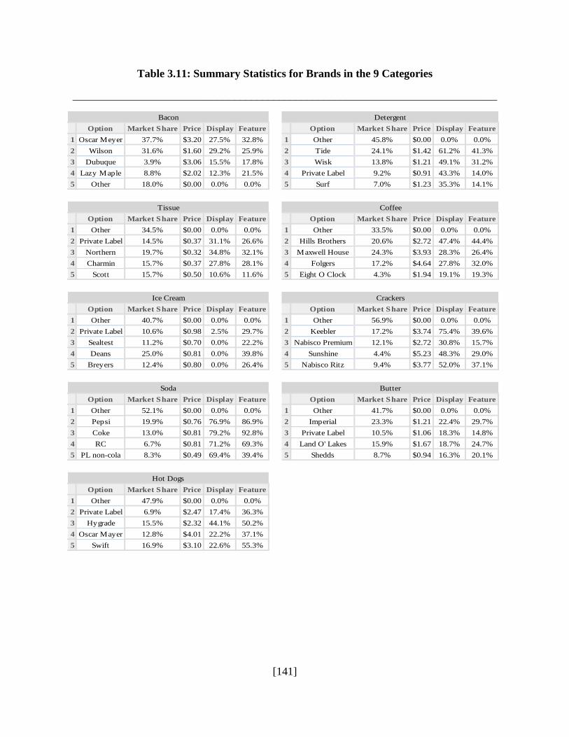
[141]

Table 3.11: Summary Statistics for Brands in the 9 Categories

____________________________________________________________________________

Option Market Share Price Display Feature Option Market Share Price Display Feature

1 Oscar Meyer 37.7% $3.20 27.5% 32.8% 1 Other 45.8% $0.00 0.0% 0.0%

2 Wilson 31.6% $1.60 29.2% 25.9% 2 Tide 24.1% $1.42 61.2% 41.3%

3 Dubuque 3.9% $3.06 15.5% 17.8% 3 Wisk 13.8% $1.21 49.1% 31.2%

4 Lazy Maple 8.8% $2.02 12.3% 21.5% 4 Private Label 9.2% $0.91 43.3% 14.0%

5 Other 18.0% $0.00 0.0% 0.0% 5 Surf 7.0% $1.23 35.3% 14.1%


1 Other 34.5% $0.00 0.0% 0.0% 1 Other 33.5% $0.00 0.0% 0.0%

2 Private Label 14.5% $0.37 31.1% 26.6% 2 Hills Brothers 20.6% $2.72 47.4% 44.4%

3 Northern 19.7% $0.32 34.8% 32.1% 3 Maxwell House 24.3% $3.93 28.3% 26.4%

4 Charmin 15.7% $0.37 27.8% 28.1% 4 Folgers 17.2% $4.64 27.8% 32.0%

5 Scott 15.7% $0.50 10.6% 11.6% 5 Eight O Clock 4.3% $1.94 19.1% 19.3%


1 Other 40.7% $0.00 0.0% 0.0% 1 Other 56.9% $0.00 0.0% 0.0%

2 Private Label 10.6% $0.98 2.5% 29.7% 2 Keebler 17.2% $3.74 75.4% 39.6%

3 Sealtest 11.2% $0.70 0.0% 22.2% 3 Nabisco Premium 12.1% $2.72 30.8% 15.7%

4 Deans 25.0% $0.81 0.0% 39.8% 4 Sunshine 4.4% $5.23 48.3% 29.0%

5 Breyers 12.4% $0.80 0.0% 26.4% 5 Nabisco Ritz 9.4% $3.77 52.0% 37.1%


1 Other 52.1% $0.00 0.0% 0.0% 1 Other 41.7% $0.00 0.0% 0.0%

2 Pepsi 19.9% $0.76 76.9% 86.9% 2 Imperial 23.3% $1.21 22.4% 29.7%

3 Coke 13.0% $0.81 79.2% 92.8% 3 Private Label 10.5% $1.06 18.3% 14.8%

4 RC 6.7% $0.81 71.2% 69.3% 4 Land O' Lakes 15.9% $1.67 18.7% 24.7%

5 PL non-cola 8.3% $0.49 69.4% 39.4% 5 Shedds 8.7% $0.94 16.3% 20.1%

Option Market Share Price Display Feature

1 Other 47.9% $0.00 0.0% 0.0%

2 Private Label 6.9% $2.47 17.4% 36.3%

3 Hygrade 15.5% $2.32 44.1% 50.2%

4 Oscar Mayer 12.8% $4.01 22.2% 37.1%

5 Swift 16.9% $3.10 22.6% 55.3%

Soda

Hot Dogs

Detergent

Coffee

Crackers

Butter

Bacon

Tissue

Ice Cream

[142]

3.7 Pricing Implications

Taking our estimated demand model as an input to the retailer’s profit maximization problem,

we calculate optimal retail prices for the 4 focal brands in each of the 9 categories. In each

category, the retailer is assumed to engage in the following maximization objective.

1{ }

1

*Pr ,Jj j

J

j j jPj

Max P c

(3.22)

where cj for each brand is assumed to obey the following rule: the average observed price of the

brand in the data implies a 20% mark-up over its cost. We call the resulting optimized retail

prices OPTPRICES and the resulting retail profit MAXPROFIT. We then re-compute the

optimal retail prices for the 4 brands taking the discrete mixed logit as the input to the retailer’s

profit maximization problem (as is usually done in the empirical IO literature, see Chintagunta

2001, Sudhir 2001 etc.). Let us call these optimized retail prices SUBOPTPRICES and the

resulting retail profit (calculated by plugging SUBOPTPRICES within our proposed demand

model) SUBMAXPROFIT. We calculate the difference between MAXPROFIT and

SUBMAXPROFIT in order to understand the retail profit implication of using our proposed

demand model, rather than the discrete mixed logit, for retail pricing. In percentage terms, this

difference turns out to be 34.4%, on average, across the 9 product categories. This is a

substantively meaningful increase in retail profit, especially considering that the retailer’s

margins are typically wafer thin. This finding becomes more significant when one considers that

our proposed model is being compared to a fairly sophisticated comparison model (discrete

mixed logit), rather than a naïve model or a subjective decision rule, for pricing purposes. For

example, Mantrala et al. 2006 use the discrete mixed logit in their retail price optimization to

[143]

compute store-specific retail prices of brands and then document a realized gross profit increase

of 30%, from the existing retail profit of the retailer, using a field experiment on 300 stores. Our

findings in this section imply that retail profit could be increased further (in our case, by 34.4%)

if the retailer used our proposed demand model as the predictive model of demand.

Next, we take our estimated demand model as an input to the manufacturer’s profit

maximization problem after assuming that the retailer uses a 20% mark-up on the wholesale

price charged by the manufacturer. In this case, we calculate optimal Bertrand-Nash equilibrium

wholesale prices for the 4 focal brands in each of the 9 categories. In each category, the

manufacturer is assumed to engage in the following maximization objective.

1{ }

1

*Pr ,Jj j

J

j j jwj

Max w c

(3.23)

where cj for each brand is assumed to be 0. We call the resulting optimized wholesale prices

(which are the fixed points to the J profit maximization problems of the J manufacturers)

OPTWPRICES and the resulting wholesale profit MAXWPROFIT. We then assess the

consequence of a single manufacturer determining their optimal price using the discrete logit

instead (while his competitors use our proposed model for pricing purposes). This “less

analytical” manufacturer’s wholesale profit decreases by 8.6%, on average, across all

manufacturers across the 9 product categories. Alternatively, if we assume that all competitors

use the discrete mixed logit, while the focal manufacturer uses our proposed demand model, this

“more sophisticated” manufacturer’s wholesale profit increases by 13.2%, on average, across all

manufacturers across the 9 product categories. Again, this is a substantively meaningful increase

in wholesale profit, especially considering the competitive pressures that exist in each category

on account of the presence of three other major brands.

[144]

These pricing implications for the retailer and the manufacturers show that our proposed

demand model serves an important managerial role beyond explicating the consumer’s choice

process using aspects that are unique to, versus shared among, various brands in a product

category (something that existing models, such as nested logit, mixed logit and probit cannot do).

This role is in determining profit-improving retail and wholesale prices for retailers and

manufacturers, respectively.

3.8 Conclusions

The mixed logit is widely used by structural modelers as a demand model for differentiated

products (see, for example, Sudhir 2001, Thomadsen 2007 etc.). The mixed logit is also used by

analytically enlightened retailers, such as Tesco (in the UK) and Kroger (in the US) for setting

product prices and promotions (see Mantrala et al. 2006 for a recent pricing application by a US

retailer). Given this, our findings in this paper about the descriptive superiority, in terms of

relaxing IIA to better capture similarity and dominance effects in demand, as well as prescriptive

superiority, in terms of yielding significantly higher retail profit when used for retail pricing, of

our proposed EBA demand model for differentiated products call for serious consideration of our

demand model as the preferred market share model for aggregate scanner data. The fact that it

reduces to the logit as a special case would lead to the standard model becoming adequate and

appropriate if warranted by the data. This should facilitate its adoption. We leave it for future

research to integrate our proposed demand model within an oligopoly model of pricing in a

distribution channel and study the implications for inferences about pricing behavior. It is

[145]

possible that inferences about price competition among manufacturers may be sensitive to

whether one uses the mixed logit or our proposed demand model as the market share model.

Another attractive modeling alternative to the mixed logit, in terms of flexibly handling

similarity and dominance effects in demand, is the market share model of Batsell and Polking

(1985). However, extending that model to include marketing variables, as well as giving the

resulting model a utility foundation, would be non-trivial challenges to overcome. If

surmountable, that line of research presents an interesting intellectual alternative to our research.

An interesting modeling extension of our proposed demand model would be to explicitly

incorporate observed brand attributes (such as package size, flavor etc.) within the model. There

is a fairly straightforward way to achieve this in our demand model. We can allow the unique

aspects to be linear functions of unique observed attributes, and the shared aspects to be linear

functions of shared observed attributes among brands, and then test whether the aspects, in fact,

end up significantly depending on these observed attributes. If one does a “variance

decomposition” of the estimated aspects into learning how much of their estimated magnitudes

can be explained using observed attributes versus how much cannot, it gives one an opportunity

to understand how consumers view brands, as in Multidimensional scaling methods. Existing

random utility models, such as the mixed logit and probit, typically lump all brand attributes,

regardless of whether they are unique to, or shared among, brands in to a linear function

specification of the brand intercepts, which is far less flexible than the aspect specification of our

proposed demand model.

Last, but not least, it would be useful to extend our proposed demand model to handle

attraction effects (as in Huber, Payne and Puto 1982, Huber and Puto 1983). Kivetz, Netzer and

[146]

Srinivasan (2004), for example, have shown how to modify existing choice models to handle the

compromise effect, another behavioral bias in consumer choices. The attraction effect remains

unaddressed so far.

[147]

3.9 References

Batsell, R. R., Polking, J. C. (1985). A New Class of Market Share Models, Marketing Science,

4, 3, 177-198.

Batsell, R. R., Polking, J. C., Cramer, R. D., Miller, C. M. (2003). Useful Mathematical

Relationships Embedded in Tversky’s Elimination By Aspects Model, Journal of

Mathematical Psychology, 47, 1, 538-544.

Ben-Akiva, M. (1973). Structure of Passenger Travel Demand Models, Ph.D. Dissertation,

Department of Civil Engineering, MIT, Cambridge, MA.

Berry, S., Levinsohn, J., Pakes, A. (1995). Automobile Prices in Market Equilibrium,

Econometrica, 63, 4, 841-890.

Chintagunta, P. K. (2001). Endogeneity and Heterogeneity in a Probit Demand Model:

Estimation Using Aggregate Data, Marketing Science, 20, 4, 442-456.

Debreu, G. (1960). Individual Choice Behavior: A Theoretical Analysis, American Economic

Review, 50, 1, 186-188.

Fader, P., McAlister, L. (1990). An Elimination by Aspects Model of Consumer Response to

Promotion Calibrated on UPC Scanner Data, Journal of Marketing Research, 27, 3, 322-332.

Gilbride, T., Allenby, G. (2006). Estimating Heterogeneous EBA and Economic Screening Rule

Choice Models, Marketing Science, 25, 5, 494-509.

[148]

Goldberg, P. (1995). Product Differentiation and Oligopoly in International Markets: The Case

of the U.S. Automobile Industry, Econometrica, 63, 4, 891-951.

Guadagni, P. M., Little, J. D. C. (1983). A Logit Model of Brand Choice Calibrated on Scanner

Data, Marketing Science, 27, 1, 29-48.

Huber, J., Payne, J. W., Puto, C. (1982). Adding Asymmetrically Dominated Alternatives:

Violations of Regularity and the Similarity Hypothesis, Journal of Consumer Research, 9, 2,

90-98.

Huber, J., Puto, C. (1983). Market Boundaries and Product Choice: Illustrating Attraction and

Substitution Effects, Journal of Consumer Research, 10, 2, 31-44.

Hui, K. L. (2004). Product Variety under Brand Influence: An Empirical Investigation of

Personal Computer Demand, Management Science, 50, 5, 686-700.

Kivetz, R., Netzer, O., Srinivasan, V. (2004). Alternative Models for Capturing the Compromise

Effect, Journal of Marketing Research, 41, 3, 237-257.

Luce, R. D. (1958). A Probabilistic Theory of Utility, Econometrica, 26, 2, 193-224.

Malhotra, N. (1984). The Use of Linear Logit Models in Marketing Research, Journal of

Marketing Research, 21, 1, 20-31.

Malkoc, S. A., Hedgcock, W., Hoeffler, S. (2013). Between a Rock and a Hard Place: The

Failure of the Attraction Effect Among Unattractive Alternatives, Journal of Consumer

Psychology, 23, 3, 317-329.

[149]

Mantrala, M., Seetharaman, P. B., Kaul, R., Gopalakrishna, S., Stam, A. (2006). Pricing

Strategies for an Automotive Aftermarket Retailer, Journal of Marketing Research, 43, 4,

588-604.

McFadden, D. (1978). Modelling the Choice of Residential Location, in Spatial Interaction

Theory and Residential Location, A. Karlquist et al. (eds.), North Holland, Amsterdam, 75-

96.

McFadden, D. (1981). Econometric Models of Probabilistic Choice, in Structural Analysis of

Discrete Data, C. Manski and D. McFadden (eds.), MIT Press, Cambridge, MA 198-272.

McFadden, D., Train, K. (2000). Mixed MNL Models for Discrete Response, Journal of Applied

Econometrics, 15, 5, 447-470.

Nakanishi, M., Cooper, L., Kassarjian, H. (1974). Voting for a Political Candidate Under

Conditions of Minimal Information, Journal of Consumer Research, 1, 2, 36-43.

Rotondo, J. (1986). Price as an Aspect of Choice in EBA, Marketing Science, 5, 4, 391-402.

Steenburgh, T. (2008). The Invariant Proportion of Substitution (IPS) Property of Discrete

Choice Models, Marketing Science, 27, 2, 300-307.

Sudhir, K. (2001). Competitive Pricing Behavior in the US Auto Market: A Structural Analysis,

Marketing Science, 20, 1, 42-60.

Thomadsen, R. (2007). Product Positioning and Competition: The Role of Location in the Fast

Food Industry, Marketing Science, 26, 6, 792-804.

[150]

Thurstone, L. L. (1927). A Law of Comparative Judgment, Psychological Review, 34, 4, 273-

286.

Tversky, A. (1972a). Elimination by Aspects: A Theory of Choice, Psychological Review, 79, 4,

42-60.

Tversky, A. (1972b). Choice by Elimination, Journal of Mathematical Psychology, 9, 4, 341-367.

essays in modeling the consumer choice process

Documents