ess' statistical learning ability - tel hai...
TRANSCRIPT

On the Statistical Learning Ability of ESs
Ofer M. Shir (Tel-Hai & Migal)Amir Yehudayoff (Technion-IIT)
[email protected] [email protected]
Foundations of Genetic Algorithms (FOGA-XIV)January 12-15, 2017, Copenhagen, Denmark
Shir (THC) & Yehudayoff (IIT) ESs’ Statistical Learning Ability FOGA-XIV 2017 1 / 37

Outline1 Introduction
ModelProbability Functions
2 The Covariance MatrixA Single Winner: (1, λ)-Selection(µ, λ)-Truncation Selection
3 The Inverse RelationProving limλ→∞ αCH = I
4 GEVD ApproximationUnveiling PDFω (J (~x))Covariance Derivation for (1, λ)-Selection
5 Simulation StudyPrimary Propositions CorroborationStatistical DistributionsValidating the Approximated Integral
Shir (THC) & Yehudayoff (IIT) ESs’ Statistical Learning Ability FOGA-XIV 2017 2 / 37
Introduction
ESs’ statistical landscape learning
Shir (THC) & Yehudayoff (IIT) ESs’ Statistical Learning Ability FOGA-XIV 2017 3 / 37

Introduction
the classical hypothesis C → H−1
• Open question since the development of ESs
• Sheer amount of empirical evidence for this relation + extensivebranding “C=inv(H)” made this hypothesis a practical postulatethroughout the years
• Recent proofs published, yet limited to Derandomization (orNatural Gradient); they exercise IGO [Akimoto2012, Beyer2014]
• Current study: “going back to basics” using first principles ofprobability theory on a classical ES model
• This work concerns the absolutely continuous case, but should stillinterest the discrete guys in the audience ...
Shir (THC) & Yehudayoff (IIT) ESs’ Statistical Learning Ability FOGA-XIV 2017 4 / 37

Introduction Model
model
quadratic approximation; optimum’s vicinity
J (~x− ~x∗) = J (~x) = ~xT · H · ~x (1)
samplingλ search-points are generated in each iteration using isotropicmutations, ~z ∼ N (~0, I);i.e., ~x1, . . . , ~xλ are independent and each is N (~0, I)
truncation selection (“winners”)
~y = arg min J(~x1), J(~x2), . . . , J(~xλ) (2)
ω = J(~y) = min J(~x1), J(~x2), . . . , J(~xλ) (3)
Shir (THC) & Yehudayoff (IIT) ESs’ Statistical Learning Ability FOGA-XIV 2017 5 / 37

Introduction Model
statistical sampling by (1, λ)-selection
1 t← 02 S ← ∅3 repeat4 for k ← 1 to λ do
5 ~x(t+1)k ← ~x∗ + ~zk, ~zk ∼ N (~0, I)
6 J(t+1)k ← evaluate
(~x
(t+1)k
)7 end
8 mt+1 ← arg min
(J
(t+1)ı
λı=1
)9 S ← S ∪
~x
(t+1)mt+1
10 t← t+ 1
11 until t ≥ Niter
output: Cstat =statCovariance(S)
Shir (THC) & Yehudayoff (IIT) ESs’ Statistical Learning Ability FOGA-XIV 2017 6 / 37

Introduction Probability Functions
probability functions
isotropic case: H = Iψ = J(~z) is a random variable obeying the χ2-distribution:
Fχ2 (ψ) =1
2n/2Γ (n/2)
∫ ψ
0tn2−1 exp
(− t
2
)dt (4)
fχ2 (ψ) =1
2n/2Γ (n/2)ψn/2−1 exp
(−ψ
2
)(5)
general case: H = UDU−1, D = diag [∆1, . . . ,∆n]
FHχ2(ψ) =∫∞
02π
sin tψ2
t cos(−tψ + 1
2
∑nj=1 tan−1 2∆jt
)×
n∏j=1
(1 + ∆2
j t2)− 1
4 dt,(6)
Shir (THC) & Yehudayoff (IIT) ESs’ Statistical Learning Ability FOGA-XIV 2017 7 / 37

Introduction Probability Functions
approximation for the general case
Fτχ2 (ψ) =Υη
Γ (η)
∫ ψ
0tη−1 exp (−Υt) dt (7)
fτχ2 (ψ) =Υη
Γ (η)ψη−1 exp (−Υψ) (8)
Υ and η account for the first two moments of ~zTH~z:
Υ =1
2
∑ni=1 ∆i∑ni=1 ∆2
i
, η =1
2
(∑n
i=1 ∆i)2∑n
i=1 ∆2i
(9)
Accuracy depends on the eigenvalues’ ∆i standard deviation.
Shir (THC) & Yehudayoff (IIT) ESs’ Statistical Learning Ability FOGA-XIV 2017 8 / 37

The Covariance Matrix
the covariance matrix
Shir (THC) & Yehudayoff (IIT) ESs’ Statistical Learning Ability FOGA-XIV 2017 9 / 37
The Covariance Matrix
the analytical form
The origin is set at the parent search-point, which is located at theoptimum:
Cij =
∫xixjPDF~y (~x) d~x (10)
PDF~y (~x) is an n-dimensional density function characterizingthe winning decision variables about the optimum.
One of the primary goals is to fully understand this expression.
Shir (THC) & Yehudayoff (IIT) ESs’ Statistical Learning Ability FOGA-XIV 2017 10 / 37

The Covariance Matrix A Single Winner: (1, λ)-Selection
winners’ density in (1, λ)-selection
Proposition 0
PDF~y (~x) = PDFω (J (~x)) · PDF~z (~x)
PDFψ (J (~x))(11)
• PDFω : density of the winning value ω
• PDF~z : density for generating an individual by mutation
• PDFψ : density of the objective function values (Eqs. 5 or 8)
sketch: consider the distribution of [~y;ω] on Rn+1
i. sample J1, . . . , Jλ according to PDFψ independentlyii. sample ~x1, . . . , ~xλ conditioned on J1, . . . , Jλ independentlyiii. ω is set to the minimum J`, and ~y is set to ~x`
Shir (THC) & Yehudayoff (IIT) ESs’ Statistical Learning Ability FOGA-XIV 2017 11 / 37

The Covariance Matrix A Single Winner: (1, λ)-Selection
simultaneous diagonalization: (1, λ)-selection
Proposition 1The covariance matrix and the Hessian commute and aresimultaneously diagonalizable, when the objective function follows thequadratic approximation.
sketch:i. the covariance reads:
Cij =
∫xixjPDFω
(~xT · H · ~x
)· PDF~z (~x)
PDFψ (~xT · H · ~x)d~x
ii. apply change of variables
U−1HU ≡ diag [∆1,∆2, . . . ,∆n] , ~ϑ = U−1~x, d~ϑ = d~x
iii. target Tij =(U−1CU
)ij
and show that it vanishes for any i 6= j dueto symmetry considerations.
Shir (THC) & Yehudayoff (IIT) ESs’ Statistical Learning Ability FOGA-XIV 2017 12 / 37

The Covariance Matrix (µ, λ)-Truncation Selection
(µ, λ)-selection
• J1:λ ≤ J2:λ ≤ . . . ≤ Jλ:λ are the order statistics obtained by sortingthe objective function values.
• ω1:λ, . . . , ωµ:λ are the first µ values from this list.
• ~y1:λ, . . . , ~yµ:λ are their corresponding vectors.
To study the covariance in this case, we consider the pairwise densityof the kth-degree and `th-degree winners (` > k):
PDF~yk:λ,~y`:λ (~xk, ~x`) = PDFωk:λ,ω`:λ (J (~xk) , J (~x`))×
×(
PDF~z (~xk)
PDFψ (J (~xk))
)·(
PDF~z (~x`)
PDFψ (J (~x`))
). (12)
Shir (THC) & Yehudayoff (IIT) ESs’ Statistical Learning Ability FOGA-XIV 2017 13 / 37

The Covariance Matrix (µ, λ)-Truncation Selection
simultaneous diagonalization: (µ, λ)-selection
Proposition 2The rank-µ covariance matrix and the Hessian commute and aresimultaneously diagonalizable, when the objective function follows thequadratic approximation.
sketch:i. the covariance reads (up to a factor):
Cij ∝∑k<`≤µ
∫xk,ix`,jPDF~yk:λ,~y`:λ (~xk, ~x`) d~xkd~x`
ii. repeat proof steps of Proposition 1 and apply the same symmetryargumentation
Shir (THC) & Yehudayoff (IIT) ESs’ Statistical Learning Ability FOGA-XIV 2017 14 / 37

The Inverse Relation
the inverse relation
Shir (THC) & Yehudayoff (IIT) ESs’ Statistical Learning Ability FOGA-XIV 2017 15 / 37
The Inverse Relation
winning values’ density & proposition 3
For simplicity, we consider (1, λ)-selection.
CDFω (v) = 1− (1− CDFψ (v))λ (13)
PDFω (v) = λ · (1− CDFψ (v))λ−1 · PDFψ (v) (14)
Proposition 3:For every invertible H and λ ∈ N, there exists a constantα = α(H, λ) > 0 such that
limλ→∞
αCH = I.
Shir (THC) & Yehudayoff (IIT) ESs’ Statistical Learning Ability FOGA-XIV 2017 16 / 37

The Inverse Relation Proving limλ→∞ αCH = I
intuition for proving proposition 3
Proposition 1 tells us that we may assume that both H and C arediagonalizable in the same base.
For a large λ, the winner ~y is close to the origin, which in turn impliesthat (CH)ii does not actually depend on i.
Shir (THC) & Yehudayoff (IIT) ESs’ Statistical Learning Ability FOGA-XIV 2017 17 / 37

The Inverse Relation Proving limλ→∞ αCH = I
proof sketch for proposition 3
i. assume H is diagonal and so off-diagonal of CH vanish
ii. Cii = E[y2i
]=∫x2iλ(1− CDFψ(J(~x)))λ−1f(‖~x‖)
iii. apply change of variables into ri =√
∆i · xi s.t.
∆iCii = cH∫r2i λ(1− CDFψ(‖~r‖2))λ−1 exp
(−J(~r)
)d~r
iv. show that α∆iCii ≥ 1− ε1 and α∆iCii ≤ 1 + ε2 (ε1 and ε2 tend tozero as λ tends to infinity)
v. for a non-diagonal H,
limλ→∞
αCH − I = limλ→∞
U (αT D − I)U−1 = 0
Shir (THC) & Yehudayoff (IIT) ESs’ Statistical Learning Ability FOGA-XIV 2017 18 / 37

GEVD Approximation
limit distributions of order statistics
Shir (THC) & Yehudayoff (IIT) ESs’ Statistical Learning Ability FOGA-XIV 2017 19 / 37

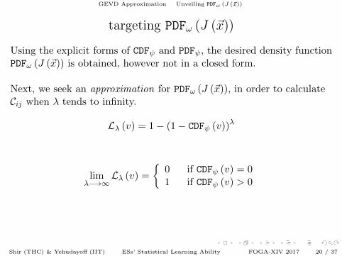
GEVD Approximation Unveiling PDFω (J (~x))
targeting PDFω (J (~x))
Using the explicit forms of CDFψ and PDFψ, the desired density functionPDFω (J (~x)) is obtained, however not in a closed form.
Next, we seek an approximation for PDFω (J (~x)), in order to calculateCij when λ tends to infinity.
Lλ (v) = 1− (1− CDFψ (v))λ
limλ−→∞
Lλ (v) =
0 if CDFψ (v) = 01 if CDFψ (v) > 0
normalization will be needed to avoid degeneracy (the distributionstend to the origin).
Shir (THC) & Yehudayoff (IIT) ESs’ Statistical Learning Ability FOGA-XIV 2017 20 / 37

GEVD Approximation Unveiling PDFω (J (~x))
von-Mises family of distributions
theorem [Fisher-Tippett]the generalized extreme value distributions (GEVD) are the onlynon-degenerate family of distributions satisfying this limit:
Lκ (v;κ1, κ2, κ3) = 1− exp
−[1 + κ3
(v − κ1
κ2
)]1/κ3
(15)
determination of shape parameter:
κ3 = limε−→0
− log2
CDF−1ψ (ε)− CDF−1
ψ (2ε)
CDF−1ψ (2ε)− CDF−1
ψ (4ε),
• If κ3 > 0, CDFψ belongs to the Weibull domain,
• if κ3 = 0, CDFψ belongs to the Gumbel domain, and
• if κ3 < 0, CDFψ belongs to the Frechet domain.
Shir (THC) & Yehudayoff (IIT) ESs’ Statistical Learning Ability FOGA-XIV 2017 21 / 37

GEVD Approximation Unveiling PDFω (J (~x))
CDFψ belongs to Weibull
Proposition 4:For the isotropic and transformed χ2 distributions, Fχ2 (ψ) , Fτχ2 (ψ),the limits exist and read κ3 = 2/n.
Corollary:Under the GEVD approximation for λ→∞, by normalizing therandom variable to v = (v − b∗λ) /a∗λ and using the tail-index result,1/κ3 = n
2 , a single winning event is described by:
CDFGEVDω (v) = 1− exp
(−v
n2
)PDFGEVD
ω (v) =n
2vn2−1 exp
(−v
n2
) (16)
Shir (THC) & Yehudayoff (IIT) ESs’ Statistical Learning Ability FOGA-XIV 2017 22 / 37

GEVD Approximation Covariance Derivation for (1, λ)-Selection
Cij approximated for (1, λ)
Cij =
∫ +∞
−∞· · ·∫ +∞
−∞xixj
n
2J(~x)
n2−1 exp
[−J(~x)
n2
]×
×1√
(2π)nexp
(−1
2~xT~x)
Υη
Γ(η)J(~x)η−1 exp (−ΥJ(~x))dx1dx2 · · · dxn
(17)
J is assumed here to satisfy J (~x) = ~xT · H · ~x ; a∗λ = F−1χ2
(1λ
):
Cij = ΦC
∫ +∞
−∞· · ·∫ +∞
−∞xixj
(~xTH~x
)n2−η ×
× exp
[Υ~xTH~x−
(~xTH~xa∗λ
)n2
− 1
2~xT~x
]dx1dx2 · · · dxn
(18)
Shir (THC) & Yehudayoff (IIT) ESs’ Statistical Learning Ability FOGA-XIV 2017 23 / 37

GEVD Approximation Covariance Derivation for (1, λ)-Selection
integration
For a general positive-definite H, the integral in Eq. 18 has anunknown closed form; it is easy to see that it commutes with H.
isotropic case H = h0I:
C(H=h0I) =Γ(n2 ) · Γ
(1 + 2
n
)· φ (n) · a∗λ
2πn/2· H−1 (19)
with
φ (n) =
πm
m! n = 2m2m+1πm
1·3·5···(2m+1) n = 2m+ 1 .
Shir (THC) & Yehudayoff (IIT) ESs’ Statistical Learning Ability FOGA-XIV 2017 24 / 37

Simulation Study
numerical validation
Shir (THC) & Yehudayoff (IIT) ESs’ Statistical Learning Ability FOGA-XIV 2017 25 / 37

Simulation Study Primary Propositions Corroboration
eigendecomposition and commutator errors10, 30, 80–dimensional separable ellipses (Hellipse)ii = c
i−1n−1 with
Niter = 105.[LEFT] c = 2 . . . 1000 using λ = 100[RIGHT] c = 2 . . . 20 over λ = 20, 100, 1000
Measure: C.E.: ‖HellipseCstat − CstatHellipse‖frob
Condition Number
n=10
n=30
n=80
Condition Number
n=10, =20λ
n=10, =100λ
n=10, =1000λn=30, =20λ
n=30, =100λn=30, =1000λ
n=80, =20λ
n=80, =100λn=80, =1000λ
Shir (THC) & Yehudayoff (IIT) ESs’ Statistical Learning Ability FOGA-XIV 2017 26 / 37

Simulation Study Primary Propositions Corroboration
the inverse relation under a large population
10, 30, 80–dimensional separable ellipses (Hellipse)ii = ci−1n−1 with
Niter = 105.[LEFT] c = 2 . . . 1000 using λ = 100[RIGHT] c = 2 . . . 20 over λ = 20, 100, 1000
Measure: I.D.: cond (HellipseCstat)− 1.0
Condition Number
n=10
n=30
n=80
Condition Number
n=10, =20λ
n=10, =100λ
n=10, =1000λn=30, =20λ
n=30, =100λn=30, =1000λ
n=80, =20λ
n=80, =100λn=80, =1000λ
Shir (THC) & Yehudayoff (IIT) ESs’ Statistical Learning Ability FOGA-XIV 2017 27 / 37

Simulation Study Statistical Distributions
statistical distributions assessment
We consider four quadratic basins of attraction:(H-1) n = 3, H1 =
[√2/2 0.25 0.1; 0.25 1 0; 0.1 0
√2]
(H-2) n = 10, H2 = diag [1.0, 1.5, . . . , 5.5]
(H-3) n = 30, H3 = diag[~I10, 2 · ~I10, 3 · ~I10
](H-4) n = 100, H4 = 2.0 · I100×100
We numerically assess the following distributions:(i) density of J(~x) over a single iteration: fτχ2
(ii) density of winning events: PDFω vs. PDFGEVDω
Shir (THC) & Yehudayoff (IIT) ESs’ Statistical Learning Ability FOGA-XIV 2017 28 / 37

Simulation Study Statistical Distributions
(i) density of J(~x) over a single iteration: fτχ2
H1 (n = 3) H2 (n = 10)
0 5 10 15 20 250
0.05
0.1
0.15
0.2
0.25
0.3
Sampling
0 20 40 60 80 100 120 1400
0.005
0.01
0.015
0.02
0.025
0.03
0.035
Sampling
H3 (n = 30) H4 (n = 100)
0 20 40 60 80 100 120 140 1600
0.005
0.01
0.015
0.02
0.025
0.03
Sampling
100 150 200 250 300 3500
0.002
0.004
0.006
0.008
0.01
0.012
0.014
0.016
Sampling
Shir (THC) & Yehudayoff (IIT) ESs’ Statistical Learning Ability FOGA-XIV 2017 29 / 37

Simulation Study Statistical Distributions
(ii) density of winning events: PDFω vs. PDFGEVDω
H1 (n = 3)(λ = 20, Niter = 105
)
0 0.5 1 1.5 2 2.50
0.5
1
1.5
2
2.5
Raw Sampling
0 1 2 3 4 5 6 70
0.1
0.2
0.3
0.4
0.5
0.6
0.7
0.8
Normalized Sampling
H3 (n = 30)(λ = 1000, Niter = 2 · 105
)
Shir (THC) & Yehudayoff (IIT) ESs’ Statistical Learning Ability FOGA-XIV 2017 30 / 37

Simulation Study Statistical Distributions
density of winning events: H2 feat. various settings(λ = 1000, Niter = 105
)
0 2 4 6 8 10 12 14 160
0.05
0.1
0.15
0.2
0.25
Raw Sampling
0 0.2 0.4 0.6 0.8 1 1.2 1.4 1.6 1.8 20
0.2
0.4
0.6
0.8
1
1.2
1.4
1.6
1.8
2
Normalized Sampling
(λ = 10000, Niter = 106
)vs.
(λ = 20000, Niter = 5 · 106
)
0 0.2 0.4 0.6 0.8 1 1.2 1.4 1.6 1.8 20
0.2
0.4
0.6
0.8
1
1.2
1.4
1.6
1.8
2
Normalized Sampling
Shir (THC) & Yehudayoff (IIT) ESs’ Statistical Learning Ability FOGA-XIV 2017 31 / 37

Simulation Study Validating the Approximated Integral
validating the approximated integral
for the isotropic case, Cstat for the 100-dimensional case (H-4) wasconstructed using λ = 5000 and over 5 · 105 iterations to obtain adiagonal with an expected value
0.5617± 0.0012
Eq. 19 obtained a value of0.5680
Shir (THC) & Yehudayoff (IIT) ESs’ Statistical Learning Ability FOGA-XIV 2017 32 / 37
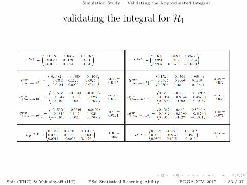
Simulation Study Validating the Approximated Integral
validating the integral for H1
Shir (THC) & Yehudayoff (IIT) ESs’ Statistical Learning Ability FOGA-XIV 2017 33 / 37

Simulation Study Validating the Approximated Integral
wrapping-up
Shir (THC) & Yehudayoff (IIT) ESs’ Statistical Learning Ability FOGA-XIV 2017 34 / 37

discussion
i. C and H commute (for any λ).this learning capability stems only from two components:(1) isotropic Gaussian mutations, and (2) rank-based selection.* learning the landscape is an inherent property of classical ESs.** it does not require Derandomization (adaptation) nor IGO (proofs)
ii. limλ→∞ αCH = I ; this approximation has two parts:(1) guaranteeing that Cstat is pointwise ε-close to C with confidence1− δ. the eigenvalues of C are at least Ω(1/λ2); for Cstat tomeaningfully approach C it requires ε 1/λ2.=⇒ number of samples required for this part is polynomial inλ, 1/ε, ln(n) and ln(1/δ).(2) guaranteeing that C is pointwise ε-close to αH−1 , α (λ,H) > 0.=⇒ upper bound on the number of samples required for this partdepends on ε, λ and on the spectrum of H.
Shir (THC) & Yehudayoff (IIT) ESs’ Statistical Learning Ability FOGA-XIV 2017 35 / 37
next steps
i. what mechanisms can increase the convergence rates?
ii. analogue phenomena near a general point:
Ei =
∫xiPDF~y (~x) d~x
Cij =
∫(xi − Ei) (xj − Ej) PDF~y (~x) d~x
similar behavior was indeed observed in simulations.
* we possess a proof sketch for the general case.
Shir (THC) & Yehudayoff (IIT) ESs’ Statistical Learning Ability FOGA-XIV 2017 36 / 37

next steps
i. what mechanisms can increase the convergence rates?ii. analogue phenomena near a general point:
Ei =
∫xiPDF~y (~x) d~x
Cij =
∫(xi − Ei) (xj − Ej) PDF~y (~x) d~x
similar behavior was indeed observed in simulations.
* we possess a proof sketch for the general case.
Shir (THC) & Yehudayoff (IIT) ESs’ Statistical Learning Ability FOGA-XIV 2017 36 / 37

Acknowledgements to Jonathan Roslund.
tak
Shir (THC) & Yehudayoff (IIT) ESs’ Statistical Learning Ability FOGA-XIV 2017 37 / 37