esl-tr-99-05-01 compilation of diversity factors and
TRANSCRIPT

ESL-TR-99-05-01
COMPILATION OF DIVERSITY FACTORS AND SCHEDULES FOR ENERGY AND COOLING LOAD CALCULATIONS
ASHRAE Research Project 1093
Preliminary Report
LITERATURE REVIEW AND DATABASE SEARCH
Bass Abushakra Jeff S. Haberl, Ph.D., P.E.
David E. Claridge, Ph.D., P.E. Energy Systems Laboratory
Texas A&M University College Station, Texas, 77843-3581
May 1999

ASHRAE RP-1093 page i
May 1999, Preliminary Report Energy Systems Laboratory, Texas A&M University
EXECUTIVE SUMMARY In this report, the first report for the ASHRAE 1093-RP project, we present: (1) our extended literature search of methods used to derive load shapes and diversity factors in the U.S. and Europe, (2) a survey of available databases of monitored commercial end-use electrical data in the U.S. and Europe, and (3) a review of classification schemes of the commercial building stock listed in national standards and codes, and reported by researchers and utility projects. The findings in this preliminary report will help us in performing the next steps of the project where we will identify and test appropriate daytyping methods on relevant monitored data sets of lighting and equipment (and other surrogates for occupancy) to develop a library of diversity factors and schedules for use in energy and cooling load simulations. The goal of this project is to compile a library of schedules and diversity factors for energy and cooling load calculations in various types of indoor office environments in the U.S. and Europe. Two sets of diversity factors, one for peak cooling load calculations and one for energy calculations will be developed. The approach to achieving these goals will be influenced by the results of each succeeding task, and our interactions with the Project Monitoring Subcommittee (PMSC). Major tasks in the approach include the following: (a) Survey existing literature on diversity factors (b) Survey existing data sets relevant to the project (c) Survey of different commercial building classification schemes (d) Survey existing statistical, analytical and empirical approaches to derive the diversity factors (e) Address the uncertainty involved in using the derived results (f) Identify the most appropriate data sets and daytyping routines to compile a library of load
shapes (g) Develop a library of load shapes, tool-kit for deriving new diversity factors, general
guidelines for using the compiled results by analysts and practitioners, and a set of illustrative examples of the use of these diversity factors in the DOE-2 and BLAST simulation programs.
In this report we describe the related literature for the ASHRAE 1093-RP project. To accomplish this we have divided the previous works into three categories: (1) existing literature on diversity factor and load shape calculations, (2) literature that reports on existing databases of monitored data in the U.S. and Europe, and (3) relevant studies about classifications of commercial buildings. In the literature on diversity factors and load shapes, we covered papers reporting the existence of databases of monitored end-uses in commercial building, methods used in developing the daytypes and load shapes, and what classification schemes were used in the commercial building sector. We report the names of the scholars and energy analysts whom we contacted in the U.S. and Europe, that provided detailed information (in a tabulated format) on existing databases on monitored end-uses in commercial buildings in the U.S. Finally, we summarize the classification schemes of the commercial building sector that are reported in national standards and codes.

ASHRAE RP-1093 page ii
May 1999, Preliminary Report Energy Systems Laboratory, Texas A&M University
We reviewed a total of 51 sources on diversity factors and load shapes from conference proceedings and scientific journals (47), internet websites (2), standards (1), and a professional handbook (1). We also consulted 10 bibliographies related to deriving load shapes, and other subjects like commercial buildings end-uses, and we reviewed methods used to calculate uncertainty analysis, that were not directly addressed in this report.
Five papers were reviewed in which the authors reported the existence of databases of monitored commercial building end-uses, from which data was utilized to develop typical load shapes. Besides these reported databases in the literature, we conducted our own search and contacts and located various sources of monitored end-uses in commercial buildings. For methods used in deriving load shapes of end-uses in the U.S., we reviewed 28 papers, one standard, one professional handbook, one thesis, and two reports on an organization websites in which the authors described (either explicitly or briefly) different methods used in daytyping weather-dependent and weather-independent end-uses, and deriving typical load shapes, that we felt could create a basis for our analysis. For methods used in Europe, we have been able to review three papers. From the literature on methods used in deriving load shapes of end-uses in the U.S., we identified 12 unique methods that were used when metered end-uses were not available, and/or employed some sophisticated techniques. Besides these methods, some other simpler methods were also reviewed. The simple methods were based on averages and standard deviations of typical daytypes, and usually utilized whenever metered end-uses existed. From the few European papers that we reviewed, only one paper described the methodology of deriving the load shapes. However, these papers are useful in providing a basis for comparison between the energy use in commercial buildings in the U.S. and Europe.
We will continue to find new methods, and will investigate the methods that we identified. We believe that those methods have a big promise in deriving the diversity factors for lighting, equipment and occupancy. We will replicate the procedures described in these methods with the most appropriate data sets. The selection criteria for the final methods to be used will be based on the usability, usefulness, accuracy, expendability, and flexibility.
In this report we also reviewed previous literature on different classification schemes that
were used in various commercial building energy-use daytyping and determination of load shapes projects. These papers reflect how utility companies and research laboratories divide the commercial building stock. We included these few papers to provide an example of commercial building classification followed in the load shape studies. We also included seven additional papers and one research report that are useful to this project, although they are not directly describing typical load profiles of commercial building end-uses. These papers give an insight on approaches that can be tested to derive the diversity factors in this project, categories of office equipment and their typical energy use, comparing engineering methods with statistical methods of deriving load shapes, and other related material.

ASHRAE RP-1093 page iii
May 1999, Preliminary Report Energy Systems Laboratory, Texas A&M University
Our review of the literature has indicated that there are several useful studies that present actual diversity factors, and provide the algorithms or procedures for deriving the diversity factors. This extensive literature review will provide us with a useful set of load shapes tools and methods for deriving diversity factors from end-use and whole-building electricity data.
On the other hand, an extensive search was conducted in order to locate and identify databases of monitored data in the U.S. and Europe. Direct contacts through e-mail, fax, and phone calls were conducted with scholars, researchers, and energy consultants, and their responses ranged from providing us with further names and references to readiness for help with or without charge to this research project. The available databases and sources of monitored lighting and office equipment data have been compiled in a tabulated format. Major sources of data were found through the ASHRAE FIND database, EPRI-CEED, ELCAP, and the Energy Systems Laboratory database that includes data monitored under the LoanSTAR program and other contracts for buildings inside and outside the state of Texas.
We also reviewed various national standards and codes, and major public surveys to identify commercial building classification schemes proposed and followed. We are proposing to follow the classification followed by the Commercial Buildings Energy Consumption Survey (CBECS), a national survey of commercial buildings and their energy suppliers, in compiling their statistics of the commercial building stock in the U.S. We based our proposal on the detailed compiled survey results of CBECS, that helped us in drawing meaningful conclusions. The CBECS classification scheme agrees with that of ASHRAE Standard 90.1, taking into consideration the small representation, in the whole commercial building stock, of the "Religious Worship" and the "Public Order and Safety" categories that appear in the CBECS classification. Therefore the commercial building classification that we will follow in developing the diversity factors and schedules for energy and cooling load calculations will consist of the following categories: (1) Offices, (2) Education, (3) Health Care, (4) Lodging, (5) Food Service, (6) Food Sales, (7) Mercantile and Services, (8) Public Assembly, and (9) Warehouse and Storage.
We will start our analysis with Office buildings (according to the RFP), and divide the Office buildings subcategory in three different groups: (1) Small (1,001 - 10,000 ft2), (2) Medium (10,001 - 100,000 ft2), and (3) Large (> 100,000 ft2).
After consultation with the PMSC, we will determine if additional categories in the
commercial building sector should be included in the study. We have located many sources of monitored commercial buildings lighting and equipment monitored data in the U.S. and some in Europe. Upon determining out the quality of the data available and its relevance to our ASHRAE 1093-RP work, and its cost, we are planning to fit the appropriate data into the defined commercial buildings categories, for the best representation of available data that meets ASHRAE PMSC needs.
In the next phases of this project we will carry out the following tasks: (1) relevant data sets to be used, (2) classification methods, (3) relevant statistical methods for daytyping and deriving diversity factors, (4) robust uncertainty analysis methodology, (5) compilation of diversity factors and load shapes, (6) development of a tool-kit and general guidelines for deriving new

ASHRAE RP-1093 page iv
May 1999, Preliminary Report Energy Systems Laboratory, Texas A&M University
diversity factors, and (7) development of examples of the use of diversity factors in DOE-2 and BLAST simulation programs.

ASHRAE RP-1093 page v
May 1999, Preliminary Report Energy Systems Laboratory, Texas A&M University
TABLE OF CONTENTS EXECUTIVE SUMMARY ............................................................................................................. i 0. INTRODUCTION ...............................................................................................................1
0.0 ........................................................................................................................... BACKGROUND........................................................................................................1
1.0 ........................................................................................................................... A
PPROACH ...............................................................................................................1 0.0 ........................................................................................................................... S
CHEDULE AND WORK PLAN.............................................................................4 1. LITERATURE REVIEW AND DATABASE SEARCH....................................................7
2.1 EXISTING LITERATURE ON DIVERSITY FACTORS AND LOAD SHAPES...................................................................................................................7 2.1.a Databases of monitored commercial building end-use loads ......................7 2.1.b Methods used in deriving load shapes .........................................................9
2.1.b.1 USA...........................................................................................10 2.1.b.2 Europe .......................................................................................24
2.1.c Classification schemes of commercial buildings.......................................26 2.1.d Other related literature ...............................................................................28 2.1.e Summary ....................................................................................................31
2.2 ANNOTATED BIBLIOGRAPHY ........................................................................37
2.3 EXISTING DATABASES OF MONITORED DATA IN THE U.S. AND EUROPE................................................................................................................50 2.3.a Contacts List in the U.S. and Europe.........................................................50 2.3.b Availability of Databases...........................................................................51
2.4 CLASSIFICATION OF COMMERCIAL BUILDINGS ......................................57
2.4.a Summary ....................................................................................................57 2.4.a.1 ASHRAE FIND ........................................................................57 2.4.a.2 ASHRAE Standard 90.1 ...........................................................57 2.4.a.3 CBECS ......................................................................................58 2.4.a.4 NAICS (new SIC) .....................................................................62 2.4.a.5 ELCAP ......................................................................................62 2.4.a.6 BECA ........................................................................................63

ASHRAE RP-1093 page vi
May 1999, Preliminary Report Energy Systems Laboratory, Texas A&M University
2.4.a.7 EPRI ..........................................................................................63 2.4.b Recommendations......................................................................................63 2.4.c Fitting Existing Databases into Commercial Buildings Categories...........64
3. PROPOSED METHODOLOGY.......................................................................................64
3.1 Relevant Data Sets .................................................................................................64 3.2 Classification Methods...........................................................................................65 3.3 Relevant Statistical Procedures for Daytyping ......................................................65 3.4 Robust Uncertainty Analysis Methodology...........................................................65 3.5 Compilation of Diversity Factors and Load Shapes ..............................................65 3.6 Development of a Tool-Kit and General Guidelines for Deriving New Diversity
Factors....................................................................................................................66 3.7 Development of Examples of the Use of Diversity Factors in DOE-2 and BLAST
Simulation Programs..............................................................................................66 0. CONCLUDING REMARKS...................................................................................................66 1. REFERENCES ........................................................................................................................66 6. BIBLIOGRAPHY..............................................................................................................72 7. APPENDIX........................................................................................................................73

ASHRAE RP-1093 page 1
May 1999, Preliminary Report Energy Systems Laboratory, Texas A&M University
1. INTRODUCTION This is the first report for the ASHRAE 1093-RP project. In this report, we present (1) our extended literature search of methods used to derive load shapes and diversity factors in the U.S. and Europe, (2) a survey of available databases of monitored commercial end-uses in the U.S. and Europe, and (3) a review of reported classification schemes of the commercial building stock used by researchers and utility projects, including those listed in national standards and codes. The findings in this preliminary report will help us in performing the next steps of the project where we will identify and test appropriate daytyping methods on relevant monitored data sets of lighting and equipment (and other surrogates for occupancy) to develop a library of diversity factors and schedules for use in energy and cooling load simulations. A thorough review of uncertainty analysis methods will be also carried out and the relevant methods will be applied to our results to help determine the required quality of the general use of the derived diversity factors. 1.1 BACKGROUND
In most office buildings, internal heat gains from people, office equipment and lighting dominate the cooling load and thus energy calculations used to calculate the cooling load. In order to estimate the impact of the internal heat sources on the energy and cooling load calculations accurately, a dynamic analysis must be performed with a computer simulation program. In many buildings, the energy use and heat gains from office equipment and lighting often deviate from peak operating conditions as people entering and leaving the building switch systems on and off. Energy using devices, also, are often switched to “standby” and “energy savings” modes during the day. Likewise, variable occupancy at the daily and weekly levels causes variable sensible and latent heat gains from people in the cooled space as well. In general these variabilities in the occupancy and operating conditions of office equipment and lighting are accounted for in building simulation programs using diversity factors and hourly schedules.
Previous studies that are relevant to this work are reviewed in this report. These studies
cover various methods used to derive load shapes, daytyping routines, and different commercial building classification schemes. Results of a survey of available end-uses is also included. This research project therefore seeks to determine the most appropriate method for calculating diversity factors from the previous literature, and, using the appropriate monitored data from U.S. and European sources, will develop a library of diversity factors for use in energy simulation programs such as DOE-2 and BLAST for energy load calculations. 1.2 APPROACH The goal of this project is to compile a library of schedules and diversity factors for energy and cooling load calculations in various types of indoor office environments in the U.S.

ASHRAE RP-1093 page 2
May 1999, Preliminary Report Energy Systems Laboratory, Texas A&M University
and Europe. Two sets of diversity factors, one for peak cooling load calculations and one for energy calculations will be developed. The approach to achieving these goals will be influenced by the results of each succeeding task (scheduled in Table 1), and our interactions with the Project Monitoring Subcommittee (PMSC). Major tasks in the approach include the following: (h) Survey existing literature on diversity factors (Tasks 1 and 2) (i) Survey existing data sets relevant to the project (Task 3a) (j) Survey of different commercial building classification schemes (Task 3b) (k) Survey existing statistical, analytical and empirical approaches to derive the diversity factors
(Task 3c) (l) Address the uncertainty involved in using the derived results (Task 4) (m) Identify the most appropriate data sets and daytyping routines to compile a library of load
shapes (Task 5) (a) Develop a library of load shapes, tool-kit for deriving new diversity factors, general
guidelines for using the compiled results by analysts and practitioners, and a set of illustrative examples of the use of these diversity factors in the DOE-2 and BLAST simulation programs (Tasks 6a, 6b, and 6c).
Tasks (a), (b), (c), and (d) have been carried out (Phase 1, and a preliminary investigation for part of Phase 2 of the project), and are reported in this preliminary report. We have also reviewed methods used for daytyping reported in the literature over the last fifteen years. The review of daytyping routines covered work performed in the U.S. and Europe. In Phase 2 of this project, after receiving the PMSC approval, we plan to test the most relevant methods by applying them to the relevant energy consumption and demand data sets. To accomplish this, we propose to test the methods with the data sets used in the Predictor Shootout I (Kreider and Haberl 1994) and the Predictor Shootout II (Haberl and Thamilseran 1996) - data that has been used by many contestants to test energy use prediction models using different statistical methods. The Predictor Shootout I and II tests will help to compare the accuracy of the different methods. The best methods will then be used to compile a library of diversity factors from the most appropriate data sets (Phase 3). Besides the previous work conducted by Haberl and Claridge (1987) which used a daily variable that consisted of counts of people entering and leaving a facility, we reviewed one additional European paper (Olofsson et al. 1998) in which the authors describe using a measured indoor CO2 ratio, which is a good measure of occupants activity, as an input in a combined Principal Component Analysis/Neural Network model to predict the energy consumption of a residential building in Sweden. In another occupancy related paper, Keith and Krarti (1999) summarized a methodology used to develop a simplified prediction tool to estimate peak occupancy rate from readily available information, specifically average occupancy rate and number of rooms within an office building. The study was carried on in a laboratory campus with three similar two and three story buildings in Boulder, CO, comprising approximately 1200 rooms, with 1174 having individual occupancy sensors. A total of 195 sensors were selected for the study. The average hourly occupancy is the monthly average of the occupancy rate in that particular hour of all workdays. To determine the peak occupancy rate, numerous combinations of linear terms were evaluated, starting with just the two independent variables of average

ASHRAE RP-1093 page 3
May 1999, Preliminary Report Energy Systems Laboratory, Texas A&M University
occupancy rate and number of rooms, and increasing the number and variety of terms to develop the best fit. A multiple linear regression model of peak occupancy rate was finally developed which is function of average occupancy rate, number of rooms, and other variables that are combinations of these two variables. The paper shows the derived average and peak typical occupancy profiles for the case study office building. This is a unique paper where the occupancy variable was measured and studied to develop typical occupancy load shapes. Otherwise, we have been unable to locate the existence of any additional data sets which could be used for energy calculations that specifically count people on an hourly basis in the same way that the electricity use of lights and receptacles is recorded at the end-use level. In the expert system that Haberl and Claridge developed for a Recreational Center consumption analysis, they created a daily occupancy parameter which, along with other parameters such as operating hours, custodian schedules, constitute a set of operational parameters (OP) that influenced the building's energy consumption. Other influencing parameters were the environmental parameters (EP), and the system parameters (SP). According to the paper, operational parameters changed on a daily basis, whereas system parameters change less frequently, otherwise they were very similar. In most of the previous work reviewed it is usually assumed that the three variables “Lighting/Receptacles /People” are considered as one variable. For this project, however, we will investigate whether or not we can break down this variable into three separate variables. Therefore, we will look in the literature for available data sets that can be correlated to an occupancy variable. The search also will be expanded to include available data sets of hourly measured data of CO2 concentration levels in office buildings. We anticipate using these data sets, if available, as a surrogate for the occupancy variable.
The LoanSTAR database which is maintained at the Energy Systems Laboratory includes several buildings with channels for monitoring the Lights/Receptacles variable, and the Lights variable separately. Therefore, we also propose to investigate a relationship between the Lights/Receptacles and the Lights variable, and develop the corresponding diversity factors in order to better understand a surrogate for an occupancy diversity factor. After identifying appropriate data sets of lighting and equipment loads in different categories of commercial buildings, and using appropriate routines for daytyping, we intend to produce a practical library of diversity factors that can be applied by practitioners. Practitioners will have access, through this study, to the hourly schedules or diversity factors that will correctly scale, in their studies, maximum expected heat gains from office equipment and lighting in commercial buildings energy and cooling load calculations. We proposed that the compiled library of the diversity factors would include the following elements:
0. Building classification methods based on existing methods such as CBECS (CBECS 1997), ASHRAE Standard 90.1 (ASHRAE 1989), and other organizations and programs, for instance, EPRI-CEED, ELCAP (ELCAP 1989), and BECA (Akbari 1994), to be approved by the PMSC.
1. Electricity use of modern office equipment, based on the work reported in literature, for instance, the “Lighting in Commercial Building” report (EIA-DOE 1992), and the RP-822 report (822-RP).
2. Typical daytypes for the appropriate office buildings.

ASHRAE RP-1093 page 4
May 1999, Preliminary Report Energy Systems Laboratory, Texas A&M University
3. Typical load profiles of occupancy and internal loads (lighting, office equipment) for each defined daytype.
4. Uncertainty factors in using the library of derived results, based on an analysis of acceptable level of uncertainty in the estimates.
5. General guidelines for practitioners and energy analysts for using the library 6. Examples of how the derived diversity factors can be input into the publicly available
simulation programs: BLAST and DOE-2. 7. Any necessary software routines used to compile the diversity factors.
1.3 SCHEDULE AND WORK PLAN The objectives of the project will be achieved by completion of three phases, as described in the RFP, with review and approval by the Project Monitoring Subcommittee (PMSC) provided after the first and second phases, before initiating the next phase. The results of Phase 1 of the project (Literature review and database search, Preliminary Report) are reported in this preliminary report.
To date, we have reviewed the literature relating to different methods for daytyping of weather-dependent and weather-independent loads in both commercial and residential buildings. We covered the residential building sector, as well, as this was useful in our evaluation of all daytyping techniques that has been used in the last fifteen years. We also reviewed daytyping methods that were used in Europe.
So far, we have located relevant data sets of monitored office equipment and lighting
loads of different types of commercial buildings in the U.S. and Europe through direct contacts (e-mail, fax, and phone calls), and also by using the ASHRAE FIND database (ASHRAE 1995) of monitored energy use. Briefly, the data sets that we located are listed below:
0. ESL: 364 monitored commercial sites, from which lighting and equipment loads are either measured or could be derived.
1. EPRI-CEED: Interior lighting monitored in 305 sites in different regions of the U.S., and "Other" end-uses from a total of 378 sites.
2. ASHRAE-FIND database: 34 sources of monitored lighting and equipment loads; each source has a sample with a size ranging from 10 to 1,000 sites.
3. Personal contacts with sources in the U.S. who promised to provide relevant data when/if they could obtain the proper release of the data from the data's owner (please refer to list of contacts in the Appendix).
4. Three European scholars and energy analysts also offered their help in proving us with relevant data from projects carried out in Europe.
5. Load shapes already derived at the Lund Institute of Technology (Sweden) for various subcategories of commercial buildings, based on an extensive monitoring project.
Phase 2, which includes the extraction of diversity factors and identification of robust uncertainty analysis methodologies, will develop a report on the testing of the derived diversity factors and schedules, and Phase 3 (Preparing a library of diversity factors and load shapes for

ASHRAE RP-1093 page 5
May 1999, Preliminary Report Energy Systems Laboratory, Texas A&M University
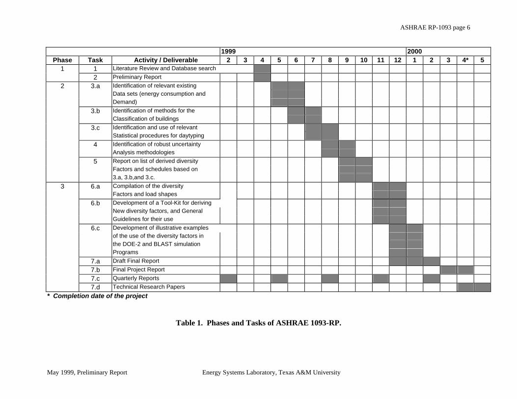
energy and cooling load calculations, Project Reports and Technical Paper) will proceed as soon as comments and suggestions about Phase 2 have been received. Table 1 below shows the scheduled phases and tasks of ASHRAE 1093-RP as proposed in our work plan.
ASHRAE RP-1093 page 6
May 1999, Preliminary Report Energy Systems Laboratory, Texas A&M University
1999 2000 Phase Task Activity / Deliverable 2 3 4 5 6 7 8 9 10 11 12 1 2 3 4* 5
1 1 Literature Review and Database search 2 Preliminary Report
2 3.a Identification of relevant existing Data sets (energy consumption and Demand) 3.b Identification of methods for the Classification of buildings 3.c Identification and use of relevant Statistical procedures for daytyping 4 Identification of robust uncertainty Analysis methodologies 5 Report on list of derived diversity Factors and schedules based on 3.a, 3.b,and 3.c.
3 6.a Compilation of the diversity Factors and load shapes 6.b Development of a Tool-Kit for deriving New diversity factors, and General Guidelines for their use 6.c Development of illustrative examples of the use of the diversity factors in the DOE-2 and BLAST simulation Programs 7.a Draft Final Report 7.b Final Project Report 7.c Quarterly Reports 7.d Technical Research Papers
* Completion date of the project
Table 1. Phases and Tasks of ASHRAE 1093-RP.

ASHRAE RP-1093 page 7
May 1999, Preliminary Report Energy Systems Laboratory, Texas A&M University
2. LITERATURE REVIEW AND DATABASE SEARCH In this section we describe the related literature for the ASHRAE 1093-RP project. To accomplish this we have divided the previous works into three categories: (1) existing literature on diversity factor and load shape calculations, (2) literature that reports on existing databases of monitored data in the U.S. and Europe, and (3) relevant studies about classifications of commercial buildings. In the literature on diversity factors and load shapes, we covered papers reporting the existence of databases of monitored end-uses in commercial building, methods used in developing the daytypes and load shapes, and what classification schemes were used in the commercial building sector. We report the names of the scholars and energy analysts whom we contacted in the U.S. and Europe, that provided detailed information (in a tabulated format) on existing databases on monitored end-uses in commercial buildings in the U.S. Finally, we summarize the classification schemes of the commercial building sector that are reported in national standards and codes. 2.1 EXISTING LITERATURE ON DIVERSITY FACTORS AND LOAD SHAPES We reviewed a total of 51 sources on diversity factors and load shapes from conference proceedings and scientific journals (47), internet websites (2), standards (1), and a professional handbook (1). We also consulted 10 bibliographies related to deriving load shapes, and other subjects like commercial buildings end-uses, and we reviewed methods used to calculate uncertainty analysis, that were not directly addressed in this report. 2.1.a Databases of monitored commercial building end-use loads
Five papers were reviewed in which the authors reported the existence of databases of monitored commercial building end-uses, from which data was utilized to develop typical load shapes including: Heidell (1984), Wall et al. (1984), Baker and Guliasi (1988), Gillman et al. (1990), and Eto et al. (1990). Pratt et al. (1990), Stoops and Pratt (1990), and Hadley (1993) also described different load methods developed with data from the ELCAP database. Akbari et al. (1994) reported on work done on monitored data collected for PG&E and the California Energy Commission (CEC).
Heidell (1984) reported on a comprehensive inventory database of end-use metered data in commercial buildings, conducted by Battelle - Pacific Northwest Laboratory. The inventory was prepared in order to develop an assessment of end-use data on existing commercial buildings and to determine the need for a public domain database. The inventory included 55 metering projects, along with the corresponding building types, location, data type, time resolution, metering technique, and availability of the data (public or private domain). The data type included the construction characteristics, occupancy characteristics (number of occupants and activity levels by day and time of day of the monitoring period), operation characteristics, equipment condition, and microclimate data. Potential data needs of six areas of research were evaluated in this study, which are: (1) utility planning, (2) building design, (3) building equipment design, (4) building energy control systems, (5) public policy, and (6) building energy use simulation techniques. However, most of the 55 listed data sources consist of a single
ASHRAE RP-1093 page 8
May 1999, Preliminary Report Energy Systems Laboratory, Texas A&M University
monitored building except some large projects such as ELCAP of Bonneville Power Administration (250 buildings), Seattle City Light commercial buildings project (11 buildings), and the California Energy Commission project (9 buildings). This study provides some guidelines as to what to look for in the current database search.
Wall et al. (1984) presented an extensive data collection effort for new energy-efficient
commercial buildings, in a continuing systematic compilation and analysis of measured data under the Building Energy-use Compilation and Analysis (BECA-CN) project at the Lawrence Berkeley Laboratory. The compiled database allows meaningful comparison of performance under different climates, occupant densities, operating hours, and internal loads. The study also aimed at correlating efficient energy usage with features of the building envelope, HVAC and lighting systems, and special operating practices, and to analyze the economics of efficient new buildings and the cost effectiveness of added energy features. The data base consisted of 124 buildings, of which 83 have one full year of measured energy usage, and 41 have design values only. Two thirds of the buildings were above 50,000 ft2. The majority of the 83 monitored buildings are large or small office buildings or schools, distributed over the five general U.S. climate zones defined by the Energy Information Administration (EIA). Since this database of monitored data did not include end-use data; only whole building metered consumption, by fuel type, its immediate use in this project may not prove fruitful.
Baker and Guliasi (1988) completed the design of a commercial end-use metering study for Pacific Gas and Electric Company (PG&E) and examined other metering studies conducted earlier. Commercial end-use metering studies were conducted for two analytic purposes: (1) building energy performance analysis, and (2) class load end-use analysis. Class load end-use studies are intended to support the estimation of end-use share, end-use intensity, and load shape (diurnal and seasonal) for the following types of building activities: (1) long-run energy and peak demand forecasts, (2) conservation and load management program assessments, (3) marketing assessments, (4) capacity planning for transmission and distribution, and (5) cost-of-service/rate design. Three distinct models of measurements for class load end-use studies are used: (1) detailed end-use measurements, which is used to establish baseline data on the composition of loads, in addition to identifying the determinants of end-use consumption, (2) summary end-use measurements, to derive class-level estimates of end-use loads for major types of commercial buildings, as well as to understand the primary determinants of loads, and (3) equipment load survey, which is used to identify the schedule and magnitude of equipment loads. PG&E's study included a very extensive end-use metering effort, and covered both residential (1,000 single-family dwellings; two to seven metered end-use in each) and commercial sectors (underway in 1988). The goals of the commercial end-use metering project were: (1) enhance PG&E's ability to establish estimates of end-use loads for important commercial customer markets, (2) focus on basic measures of end-use consumption that would enhance PG&E's ability to reliably model the interactions among major end-use loads, the effect of fuel substitution, and the effects of changing service requirements, and (3) to develop data series that adequately represent diversity within the priority commercial customer markets. The study was designed to cover high priority commercial segments from fourteen business types defined by PG&E covering its six operating regions. The categories to be covered were: (1) Offices, Non-food Retail, (3) Food Retail, (4) Restaurants, and (5) Warehouses. PG&E could be contacted for access to their commercial building data during our analysis in Phase 2 of the project.

ASHRAE RP-1093 page 9
May 1999, Preliminary Report Energy Systems Laboratory, Texas A&M University
Gillman et al. (1990) reported on the End-use Load and Consumer Assessment Program (ELCAP) which collected hourly metered and associated characteristics data for approximately 400 residential and commercial buildings equipped to meter hourly electricity consumption for up to 16 end-uses in residences, and 20 end-uses in commercial buildings. In their paper the authors described four building types: (1) Single-Family Residential (68 buildings), (2) Single-Family Model Conservation Standards (21 buildings), (3) Commercial Office (9 buildings), and (4) Commercial Retail (9 buildings). In the residential sector the end-uses were: (1) Heating, Ventilating, Air Conditioning (HVA), (2) Hot Water (HO), and (3) all Other (OTH). In the commercial sector the end-uses included: (1) Heating, Ventilating, Air Conditioning (HVA), (2) Lighting (TCL), and (3) all Other (TCO). Average load shapes were created, in the ELCAP study, for each building type and end-use by averaging hourly electricity consumption data across sites. Bonneville Power Administration (who performed the ELCAP program) could be contacted for access to their commercial building data during our analysis in Phase 2 of the project. Eto et al. (1990) identified 27 end-use metering projects in the U.S., eleven of which are in the commercial building sector. Sample sizes ranged between 7 and 105 buildings, and included 15 minutes, 30 minutes and hourly data. This paper offers some help as to where to locate sources of commercial building monitored data. Besides these reported databases in the literature, we conducted our own search and contacts and located various sources of monitored end-uses in commercial buildings. The findings are reported in section 2.3 of this report. 2.1.b Methods used in deriving load shapes For methods used in deriving load shapes of end-uses in the U.S., we reviewed 28 papers, one standard, one professional handbook, one thesis, and two reports on an organization websites in which the authors described (either explicitly or briefly) different methods used in daytyping weather-dependent and weather-independent end-uses, and deriving typical load shapes, that we felt could create a basis for our analysis. The papers and other literature included: Akbari et al. (1988), Norford et al. (1988), Parti et al. (1988), ASHRAE (1989), Eto et al. (1990), Finleon (1990), Schon and Rodgers (1990), Stoops and Pratt (1990), ASHRAE (1991), Katipamula and Haberl (1991), Bronson et al. (1992), Mazzucchi (1992), Rohmund et al. (1992), Hadley (1993), Akbari et al. (1994), Halverson et al. (1994), Hamzawi and Messenger (1994), Jacobs et al. (1994), Margossian (1994), Norford et al. (1994), Szydlowski and Chvala (1994), Thamilseran and Haberl (1994), Wilkins and McGaffin (1994), Bou-Saada and Haberl (1995), CEED (1995), Bou-Saada et al. (1996), Emery and Gartland (1996), Katipamula et al. (1996), Nordman et al. (1996), Parker (1996), EPRI (1999), Keith and Krarti (1999), and Thamilseran (1999). For methods used in Europe, we have been able to review three papers that included: De Almeida et al. (1998), Noren and Pyrko (1998), and Olofsson et al. (1998).

ASHRAE RP-1093 page 10
May 1999, Preliminary Report Energy Systems Laboratory, Texas A&M University
2.1.b.1 USA
The Energy-use Disaggregation Algorithm (EDA) developed by Akbari et al. (1988) is an engineering method which primarily utilizes the statistical characteristics of the measured hourly whole-building load and its statistical dependence on temperature. In the EDA the sum of the end uses is constrained at hourly intervals to be equal to the measured whole-building load, providing a reality check not always possible with pure simulation. The primary component of the EDA is the regression of hourly load with outdoor dry bulb temperature. Two season-specific (summer and winter sets of temperature regression coefficients are used to cover the temperature dependency of the building load. Twenty-four regression models (one for each hour) are developed for each season. The temperature regression equations are used to separate the load predicted by the regression, LREG, into a temperature-dependent part, LTD, and a temperature-independent part, LTI. The temperature-dependent load is attributed to space conditioning equipment. The temperature-independent load is the sum of loads such as lighting and miscellaneous equipment, as well as temperature-independent cooling at the base temperature TBASE. The temperature-independent load is then prorated according to the loads predicted by a simulation developed based on a building audit. If the actual load at a particular hour on a particular day does not perfectly lie on the best-fit regression line, so the difference ∆, between the actual load LACT and LREG is split between the two parts of the load, and end-use profiles for average summer and winter days are developed. The EDA method was applied to buildings in the cooling mode (seven buildings in Southern California). It does not account for nonlinearities of load, latent load, heat storage, special load management options such as cool storage and daylighting, and temperature or seasonal dependencies in end-uses other than conditioning. However, the intent of the method is to supply reasonable end-use breakdowns when detailed information is scarce. This method is a hybrid method that uses monitored data, statistical disaggregation, and prorating based on a simulation. The method is fundamental and will be tested in our analysis.
In a study limited to the Office building subsector, Norford et al. (1988) investigated the
measured power densities and load profiles of personal computers and their immediate peripherals such as printers and display terminals. They used portable power meters to make short-term measurements of the actual power requirements of the equipment in both active operation and stand-by mode. The authors found that nameplate ratings overstate actual measured power by factors of 2 to 4 for PCs and 4 to 5 for printers, and thus using nameplate ratings in demand projections and building design decision can be misleading. A typical weekday load profile of internal loads was generated for a 12,000 m2 office building, but included both plug loads and lighting. The authors did not elaborate on how the typical profile was generated, but yet, the study represent an early attempt at using typical load shapes for understanding trends in energy use and opportunities for efficiency for electronic office equipment. This paper may not prove very useful in our project.
Parti et al. (1988) used a Conditional Energy Demand (CED) technique which allows for the development of an estimate residential appliance-specific energy usage and conservation effects without placing end-use meters on the appliances. End-use metered consumption information were used only for comparison to the CED estimates of end-use load shapes. The specific purposes of this load research project were: (1) to measure the contribution to system hourly load of the residential class, (2) to measure the components of this load resulting from the

ASHRAE RP-1093 page 11
May 1999, Preliminary Report Energy Systems Laboratory, Texas A&M University
operation of room ACs and refrigerators on the peak day, (3) to determine the effect of substituting more energy efficient ACs and refrigerators, and (4) to attempt to develop a model for estimating end-use profiles based on total load and demographic data without the need for end-use metering.
The CED carries out the disaggregation of the total load into its end-use components by applying Multiple Linear Regression (MLR) analysis to a data set composed of total load data, survey and weather information. In the MLR estimating equation, the hourly residential load, Eh, is written as the sum of the hourly end-use demand functions for room AC, frost-free refrigerators, non-frost-free refrigerators, pool pumps, central AC, an "unspecified" category, at hour "h". In the MLR model, the hourly AC variable is obtained using regression models function of building thermal mass temperatures, building indoor air temperature, and energy consumed by end-uses other than AC. The refrigerators variables are also obtained using regression models function of the capacity of the refrigerators. The model breaks down the hours of the day into four general hourly categories: (1) Night (12AM-6AM), (2) Morning (7AM-9AM), (3) Midday (10AM-5PM), and (4) Evening (6PM-11PM). Load shapes were developed based on the MLR model and the time categories schemes. This is a statistical method that will be investigated in our analysis.
ASHRAE Standard 90.1 (ASHRAE 1989, Table 13-3), lists diversity factors obtained
from a study conducted at Pacific Northwest Laboratory "Recommendation for Energy Conservation Standards and Guidelines for New Commercial Buildings, Vol. III, App. A., PNL-4870-8, 1983". The compiled table includes diversity factors for: (1) Occupancy, (2) Lighting and Receptacles, (3) HVAC, and (4) Service Water Heating (SWH). Three load shapes (Weekday, Saturday, Sunday) were included for each of the following categories: (1) Assembly, (2) Office, (3) Retail, (4) Warehouse, (5) School, (6) Hotel/Motel, (7) Restaurant, (8) Health, and (9) Multi-Family. No details on the method used in developing these diversity factors were reported in ASHRAE Standard 90.1. However, we will use these diversity factors for comparison reasons with our results.
Eto et al. (1990) discussed the importance of end-use load shape data for utility integrated resource planning, summarized leading utility applications and reviewed the latest progress in obtaining load shape data. The paper suggested that the most promising avenue for cost-effective development of end-use load shape data is an optimal combination of data transfer, simulation, statistical analysis, and end-use metering. The main applications of load shape data include: (1) Demand-side management, (2) Forecasting, and (3) Integrated resource planning.
The authors mentioned that prior to recent end-use metering projects, the only means for obtaining load shapes was the estimation methods relying extensively on engineering judgement to create a single prototype that represent the energy use of a certain building stock, using hourly simulation programs. These simulated end-use load shapes were calibrated at an extremely high level of end-use and temporal aggregation similar to monthly utility bills. The paper described six different methods used in load shape estimation: (1) one dimension application of the Stephan-Deming Algorithm (SRC 1988, ref. Eto et al. 1990), (2) the variance allocation approach (Schon and Rodgers 1990), (3) the End-use Disaggregation Algorithm (EDA) (Akbari et al 1988), (4) the Conditional Demand Approach (Parti and Parti 1980, ref. Eto et al. 1990), (5)

ASHRAE RP-1093 page 12
May 1999, Preliminary Report Energy Systems Laboratory, Texas A&M University
the bi-level regression approach (SSI 1986, ref. Eto et al. 1990), and (6) the Statistically Adjusted Engineering approach (SAE) (CSI, CA, ADM 1985, ref. Eto et al. 1990).
Methods (1) to (3) are Deterministic Methods and rely on exact reconciliation to an hourly control total, which is provided by the hourly whole-building load research data. The starting point for the reconciliation is an engineering simulation of the sort relied upon by the earliest load shape estimation methods. The methods typically rely on much more detailed information to develop the simulation input (minimizing the extensive reliance on engineering judgement). Method (1), the one-dimensional application of the Stephan-Deming Algorithm, is the most straightforward allocation method, and is basically a simple proration of the difference between the observed total and the sum of the simulated end-uses based on the magnitude of the original simulated estimates. This approach has been used to estimate commercial sector end-use load shapes for the Southern California Edison Company. Eto et al. did not elaborate in explaining the details of this method, but we will investigate it in our analysis. Method (2), the variance allocation approach, is also an allocation rule, and involves prorating the difference between the simulated and control totals based on the observed statistical variation in the simulated end-use loads. The basic intuition for this approach is that loads which are highly variable are more likely to account for any differences between a point estimate (simulated) of their magnitudes than loads which are relatively stable. This approach was applied to a study of commercial buildings in the Florida Power and Light Company service territory. This approach is explained further in (Schon and Rodgers 1990), below, and will be considered in our analysis. Method (3), the End-use Disaggregation Algorithm is described in (Akbari et al. 1988), above, and was used to develop end-use utilization intensities (EUIs) and load shapes for commercial buildings in the Southern California Edison service territory. This approach is detailed in (Akbari at al. 1988) above. Methods (4) to (6) are Statistical Methods, and typically rely on regression techniques that correlate explanatory variables with the hourly control total. These variables need not all be physical and the reconciliation to the control total is usually expressed in goodness of fit. Method (4), the Conditional Demand Approach is essentially a correlation analysis of the energy use of many separate premises against the energy using equipment in each of these premises. The analysis seeks to determine the difference in observed load due to the presence of a given energy-using device, all other things being held equal. The difference is taken to be the energy contribution of the device. The technique was first applied to annual and monthly billing data. With the availability of whole-building load shape data, the technique was extended to an hourly time step. This approach is explained in more details in (Parti et al. 1988) above. Unfortunately, purely correlational methods for end-use load shape estimation can ignore engineering principles that affect energy use (like weather effect on heating and cooling loads). Hybrid statistical methods have been introduced to account for this factor. The first method,

ASHRAE RP-1093 page 13
May 1999, Preliminary Report Energy Systems Laboratory, Texas A&M University
Method (5), is called the bi-level regression approach involves two levels of time series and cross section regression analyses. In the first level, the hourly load of individual households is regressed against both weather-related variables, and sine and cosine functions which capture daily, weekly, and seasonal periodicity in loads that are independent of weather.
In the second level, the coefficients estimated in the first level (separately for each household) are regressed as a group against customer characteristics. The second method, Method (6), is called the Statistically Adjusted Engineering approach (SAE), and is very close to the Deterministic methods. First an engineering simulation is developed to provide an initial estimate of end-use loads. Next, the initial estimates are regressed against control totals, which are averages of hourly energy use for typical days. The estimated coefficients can then be thought of as adjustment factors that reconcile the initial estimates to the control total. In other words, correlational analysis is used to perform the allocation of differences statistically, whereas, in the deterministic methods the allocation is performed deterministically. In this paper, the authors noted based on their experience, that the mean end-use loads tend to stabilize with sample sizes of about 20. This valuable note will be investigated and used as a reality check in this project.
Finleon (1990) mentioned that experience has shown that end-use metering which is a traditional method for obtaining end-use load shapes is expensive, data intensive and time consuming. The paper describes a methodology whereby end-use load shapes for residential and commercial/industrial buildings can be developed without undertaking a new end-use metering project. In the residential sectors load shapes were developed for the following end-uses: (1) electric heating, (2) refrigerators, (3) electric dryers, (4) electric water heating, (5) air conditioning, (6) freezers, (7) cooking, and (8) other. The commercial/industrial subcategories included: (1) Offices, (2) Restaurants, (3) Warehouses, (4) Health Facilities, (5) Manufacturing, (6) Retail, (7) Grocery Stores, (8) Schools & Colleges, (9) Hotel/Motels, and (10) Miscellaneous. In the commercial/industrial sector, load shapes were developed for the following end-uses: (1) Electric heating, (2) lighting, (3) refrigeration, (4) air conditioning, (5) water heating, and (6) other. The methodology used in developing the end-use load shapes consisted of the following steps: (1) obtain hourly load research data by customer segment, (2) obtain energy use history by customer segment, (3) combine load research data with energy use history to obtain magnitude of customer segment load shape, (4) obtain initial end-use load shapes for each customer segment, (5) obtain average annual energy use estimates by end-use for each customer segment, (6) obtain saturation data for each end-use by customer segment, (7) combine initial load shape with average energy use and saturation data and reconcile to total customer load shape to obtain first estimate of the total magnitude of the end-use load shapes, and finally (8) review and adjust end-use load shapes until "reasonable". This method is basically developed to overcome the problems associated with end-use metering, and is based on reconciling estimated end-uses load shapes with average end-uses load shapes developed for corresponding customer segment (minimizing sum of the squares), "borrowed" from external sources. The method can be helpful in our analysis, in the cases of having only metered whole-building energy use.
To provide a cost-effective alternative to end-use metering for electric utilities, Schon and Rodgers (1990) have applied a hybrid engineering/statistical approach to end-use load shape estimation for the commercial sector. The authors developed a method which: (1) identifies

ASHRAE RP-1093 page 14
May 1999, Preliminary Report Energy Systems Laboratory, Texas A&M University
systematic biases in engineering model hourly end-use load estimates, (2) adjusts the engineering model to significantly reduce these biases for individual building end-use estimates, (3) uses a variance-weighted approach to reconcile adjusted engineering estimates with whole-building metered data, and (4) offers to estimate end-use load shapes at an order of magnitude less cost than that end-use metering.
The authors stated that end-use metering alone provides only descriptive data and
provides no predictive modeling component. Alternatively, the engineering models provide the predictive modeling component missing from the end-uses. Moreover, the statistical methods that rely on existing end-use and whole building hourly loads have the advantage of capturing the behavioral components of the building operation, in the whole building load variations. Thus, the hybrid method combines the advantages of both engineering and statistical methods. The methods was applied for work at Florida Power and Light (FPL). Hourly data which was collected in 457 statistically sampled commercial facilities. Biases in the engineering models of end-uses, developed using ASHRAE CLTD method, were identified from regressing whole-building metered loads on individual end-use load estimates at each hour. Finally, to reconcile the sum of the hourly end-use load estimates with each individual facility's hourly research data, using the variances observed for each regression coefficient. The difference between simulated and metered totals is prorated based on statistical variation in the simulated end-use loads. The largest and most variant end-uses receive the largest portion of the difference between the engineering simulation and the metered whole-building load. This method is well explained very helpful in deriving load shapes of end-uses when metered end-uses are not available.
Stoops and Pratt (1990) reported a comparison between load shapes developed for a
sample of 14 office buildings metered under the ELCAP project and ASHRAE Standard 90.1 standard profiles. In the ELCAP office load shapes, a "specialized" averaging technique (not described in the paper) was used to maintain the prototypical "hat" shape. The lighting load profile based on ELCAP metered data shows that around 20% of the installed lighting capacity is in use before 8:00 AM, whereas ASHRAE profile shows zero load. Between 9:00 AM and 6:00 PM, ELCAP shows 75% of the capacity in use, whereas ASHARE shows 90%, instead. In the Equipment load profile, ELCAP shows that 50% of the installed equipment capacity is in use before 6:00 AM compared with 0% for ASHRAE. The authors argued that ASHRAE profiles are designed to represent new construction. The method of deriving the load shapes in this paper was not described, and therefore the paper has no immediate benefit for our project. However, comparing the ELCAP load shapes with those of ASHRAE showed important features that should be considered, such as the electricity use in the non-occupied hours of offices.
In the Handbook of HVAC Applications (ASHRAE 1991), load shapes are displayed for
general categories for buildings, for instance, office buildings and warehouses. For example the load profile of the Office buildings is shown to peak at 4:00 P.M. That of the warehouse peaks at 10:00 A.M. to 3:00 P.M. These load profiles could be used in buildings analyzed for heat recovery. Load profiles for two or more energy forms during the same operating period may be compared to determine load-matching characteristics under diverse operating conditions. These curves, together with the load duration curves (accumulated number of hours at each load condition from highest to lowest load per day, month, or a year) will be useful in energy consumption analysis calculations as a basis for hourly input values in energy simulation
ASHRAE RP-1093 page 15
May 1999, Preliminary Report Energy Systems Laboratory, Texas A&M University
programs, and will therefore be considered for inclusion in the library of profiles. However, it is worth noting that it was not mentioned where these ASHRAE profiles came from or how they were estimated or derived.
Katipamula and Haberl (1991) identified typical daytypes for a building, using monitored
non-weather-dependent electricity use. Load shapes were generated from the data for each typical daytype and used as schedules in a DOE-2 building energy simulation model. In deriving the daytypes, the mean and the standard deviation of the energy use at each hour for the entire data group were calculated, and a Regularity Index (RI) was calculated and checked against a maximum acceptable value (10%) for each hour. If the RI for all 24 hours exceeds the 10% value, hourly data is summed to daily totals and the mean and standard deviation of the daily consumption are calculated. Three daytypes are then identified as follows: (1) LOW-D days with daily consumption lower than Y (10%) times one standard deviation below the mean; (2) HIGH-D days with daily consumption higher than Y times one standard deviation above the mean; (3) NORMAL-D , the remaining days. The daytypes were then subdivided to LOW-LOW D, LOW-HIGH D, LOW-NORMAL D, HIGH-LOW D, HIGH-HIGH D, HIGH-NORMAL D, NORMAL-D, NORMAL-LOW D, AND NORMAL-HIGH D. As a result, the hourly load average profile for each daytype was generated. The procedures in this paper are unique, and although simpler than Thamilseran and Haberl (1994) will be considered further for this project. Bronson et al. (1992) used four different daytyping procedures together with a comparative three-dimensional graphical inspection technique to calibrate a DOE-2 simulation to non-weather-dependent loads. The daytyping methods used were: (1) the default DOE-2 daytype profiles from the reference manuals; (2) the ELF-OLF daytype profiles which are based on techniques outlined by Haberl and Komor (1990a, b); (3) the daytyping based on a two-weeks of energy audits, averaging the Monday-through-Friday profiles into a Weekday profile, and Saturday and Sunday profiles into a Weekend profile; and (4) the daytyping approach of Katipamula and Haberl (1991). The study showed that the results using DOE-2 daytype profiles were outperformed by the results of all other methods when the simulated data was compared against the monitored data. This paper provides valuable advice concerning the input of different daytypes on a large office building simulated with DOE-2. Mazzucchi (1992) described a Deterministic technique for determining building end-use energy consumption profiles applied to the DOE Forrestal Building. A hybrid approach was used combining short-term (24 hour) monitoring of a subset of the 131 panels supplying electricity to the fluorescent lights., with instantaneous measurements from all of the remaining panels in the building. The procedure appeared promising due to the regularity of the total building electric load profiles over the year, and the fact that heating and cooling were not provided the building's electrical service. One-time measurements of occupied and unoccupied periods were performed with portable voltage and current meters. The plug transformer loads were subtracted from the totals for each panel and the net lighting load was obtained. Subsequent steps split the logger files by panel and created individual profiles. Missing data were filled as necessary to create 24 hours profiles. Summations were then performed, producing for the monitored sample of panels a profile for occupied hours and another for unoccupied hours. For the weekend profile, only 9 individual panel profiles were collected, while for weekdays 50 profiles were available. Accordingly the weekend profile was slightly

ASHRAE RP-1093 page 16
May 1999, Preliminary Report Energy Systems Laboratory, Texas A&M University
more variable in shape and smoothness than the weekday profile. The diversity of profiles from 50 panels produced a profile that was smooth through all hours and flat during fully occupied and unoccupied hours. The one-time measurements were summed, producing a single value for lighting power consumption in occupied hours and another value for unoccupied hours. The next step combined the collected profile summations with the one-time measurements to produce a total building profile for a typical working and a typical nonworking day. The procedure maintained the profile shapes as collected but adjusted them to reflect the power as recorded from the one-time measurements. In a similar manner, the plug load transformer loads for the entire building were calculated. This paper describes a simple method of deriving load shapes of metered end-uses based on averages for the weekdays and the weekends.
Rohmund et al. (1992) described an end-use disaggregation approach and reported the
results of two studies. In the first study completed for a southern utility, end-use load shapes were estimated for each 450 buildings in a statistical sample. The second study performed for a mid-Atlantic utility, covered a sample of government and private office buildings. The approach combined engineering estimates and hourly whole-building loads with a statistical adjustment algorithm, offering an economical method for developing commercial end-use load shapes. The steps of the approach are: (1) sample selection, where whole-building electricity consumption is metered and analyzed for each site, (2) on-site surveys, where information about lighting and equipment inventories and schedules is gathered, (3) survey analysis, where engineering end-use load shapes are constructed and statistically adjusted, using the survey data and the metered whole building-data, and (4) database preparation, where the adjusted shapes for each case are combined in a single database and organized under building types, rate class, or other customer segments. Deriving the load shapes of weather-dependent and weather independent loads in this paper was based on the EDA approach described by Akbari et al. (1988). Four different daytypes were determined: (1) typical weekday, (2) typical weekend, (3) cold day, and (4) hot day. This paper has no immediate benefit in our analysis, since the load shape method used is not unique, but illustrates the use of a well-defined method (EDA).
Hadley (1993) employed a Temporal Synoptic Index (TSI) approach for weather-
dependent data which uses a combination of principal component analysis (PCA) and cluster analysis on the resultant principal components (PC’s), to identify days which are considered meteorologically homogeneous. He used this technique to determine the response of the HVAC system of four buildings, monitored as part of ELCAP, to different weather conditions. Once the number of daytypes has been specified, each day in the data set analyzed can be assigned to a specific, unique daytype and the average values of each meteorological variable calculated for each daytype. The weather data was obtained from the National Weather Service (NWS). Each weather-daytype was defined in terms of the daily average of the dry-bulb and wet-bulb temperature, extraterrestrial and total global horizontal radiation, clearness index, and wind speed. The unique character of each weather daytype was established by: (1) the mean value of each of the original weather variables within each daytype; (2) the frequency of occurrence of the daytype by month; and (3) the diurnal variation of each variable within each daytype. However, twenty different daytypes were specified arbitrarily which resulted in some daytypes that were not significantly different from others. Finally, average hourly heating and cooling profiles were generated for each of the weather daytypes for three different buildings. In a similar fashion as Bou-Saada and Haberl (1995), this paper describes a very sophisticated

ASHRAE RP-1093 page 17
May 1999, Preliminary Report Energy Systems Laboratory, Texas A&M University
weather-daytyping routine that may prove useful for application for deriving diversity factors from weather dependent whole-building loads. Akbari et al. (1994) applied an end-use load shape estimation technique to develop annual energy use intensities (EUI’s) and hourly end-use load shapes (LS’s) for commercial buildings in the Pacific Gas and Electric company (PG&E) service territory. The results were ready to use as inputs for the commercial sector energy and peak demand forecasting models used by PG&E and California Energy Commission (CEC). First, the initial end-use load shape estimates were developed with DOE-2 using building prototypes based on surveys. Then average measured whole-building load shapes and annual energy use intensities were derived. The initial end-use load shapes were reconciled with the measured whole-building load shape data, by applying the End-use Disaggregation Algorithm (EDA) to obtain reconciled end-use LS’s and corresponding EUI’s. Secondly, the reconciled EUI were combined with additional analysis of the DOE-2 prototypes and additional information from on-site surveys to specify a complete set of revised energy use input for the CEC and PG&E models. Developing these inputs involved: (1) development of EUI’s for electric heating and non-electric end uses; (2) expressing reconciled EUI’s relative to a base year; (3) accounting for fuel saturation effects; (4) accounting for office equipment EUI’s; (5) disaggregating reconciled EUI’s by building and equipment vintage; (6) accounting for the impact of equipment energy efficiency; and (7) accounting for climatic impact on space-conditioning EUI’s. The approach developed by Akbari has several interesting techniques that may prove useful for this project. The EDA method (reported above) will be one of the methods that we will test.
Halverson et al. (1994) developed a short-term monitoring strategy in a study they conducted at the DOE Forrestal Building to: (1) assist in the development of the Shared Energy Savings (SES) request for proposal (RFP) from potential lighting retrofit contractors, and (2) provide empirical data that could be used to confirm predicted results. To accomplish these goals, three distinct but integrated monitoring activities were planned: (1) baseline monitoring of the existing lighting loads, (2) performance monitoring of any proposed lighting retrofit, and (3) post-retrofit monitoring of the new lighting loads. The results of the baseline monitoring were detailed weekday and weekend end-use profiles of the Forrestal electrical consumption. The developed lighting load profile showed that a large amount of lighting occurs 24 hours a day, thus lighting is left on continuously. Post-retrofit monitoring also resulted in weekday and weekend profiles, that showed savings of 55.4% and 57.4% in daily consumption respectively. The paper did not elaborate on how the load profiles were developed and therefore has no immediate benefit in our work. However, it illustrates how an actual load profile may deviate from a typical load profile, whenever there is an improper use of lights or equipment in a certain building.
Hamzawi and Messenger (1994) undertook a project to develop estimates of energy savings and peak demand impacts from the implementation of a host of DSM technologies in 16 commercial and two residential building types. The project was conducted for the California Conservation Inventory Group (CCIG). The overall approach employed involved: (1) collecting data for establishing baseline residential Unit Energy Consumption (UEC), commercial Energy Utilization Intensity (EUI), and average load shape information by building type, vintage, and climate region, (2) collecting and analyzing data to establish base case residential and

ASHRAE RP-1093 page 18
May 1999, Preliminary Report Energy Systems Laboratory, Texas A&M University
commercial building prototypes by building type, vintage, and climate region, (3) simulating energy use from the base case prototypes (using DOE-2.1 program) and reconciling the results with the baseline UEC and EUI, and load shape data for each building type, vintage, and climate region, (4) screening initial list of measures, and developing or selecting the appropriate methodology to analyze and quantify the energy savings, coincident peak demand impacts, and load shapes for each technology, (5) developing programs to process, manage, and store the large amounts of input and output data associated with the estimation of the impacts for all measures, (6) developing the parametric cases associated with the description and application of each measure to the appropriate building types, vintages, and climate regions, and (7) utilizing the base cases and parametric cases, the selected methodology, and the data processing and management programs to estimate the energy savings, coincident peak demand impacts, and load shapes associated with each conservation measure. The paper did not describe any specific method in deriving load shapes, but illustrates the calibration of DOE-2 simulations with load shapes, EUI's, and UEC's. It is not of major benefit in our work.
To reduce the costs associated with true power measurements, Jacobs et al. (1998) developed surrogate measurements techniques. Specialized data loggers were used to monitor some easily observed parameters such as fixture on/off status, fixture light output, or lighting circuit current. This information combined with measurements of lighting fixture power was used to estimate energy consumption and savings resulting from lighting measures. Cost savings from the surrogate measurements resulted from lower hardware costs, lower installation costs, and reduced data analysis costs. In a case study conducted by the authors an estimate of lighting energy consumption in a small office building (3,800 ft2) using fixture status measurements was compared to true electric power measurements on the same set of fixtures over the same monitoring period. Each data logger was downloaded and time-series measurements of fixture on/off status were multiplied by the connected load represented by each sample point. These data were summed to obtain a full building load shape and compared to the true electric power measurements.
Margossian (1994) used a heuristic pattern recognition algorithm to disaggregate
premise-level load profiles. This algorithm, the Heuristic End-use Load Profiler (HELP) uses as input 5-minute or 15 minute residential premise-level load data; it also requires as input connected load estimates of the cooling, heating and water heating appliances. HELP will then generate 5-minute or 15-minute residential cooling, heating, and water heating load profiles for every premise and every day in the sample used. The algorithm first scans the premise-level load profile and identifies all spikes in the profile that are large enough with respect to the connected load of the space conditioning appliance, and categorizes these spikes with various attributes such as shape, timing, magnitude, and duration. In a second stage, the classification stage, the algorithm decides whether or not to attribute each of the identified spikes to the space conditioning appliance. The resulting spikes comprise the end-use load profile for the space conditioning appliance on that day. The load profile of the water heating appliance is derived from the residuals of the premise-level load profile, after subtracting the space conditioning appliance load profile, using the scanning and classification stages. The end-use disaggregation procedure described in this study, although not immediately useful, may be of use in providing diversity factors from a whole-building data set.

ASHRAE RP-1093 page 19
May 1999, Preliminary Report Energy Systems Laboratory, Texas A&M University
To calibrate a DOE-2 model, Norford et al. (1994) used meters on the electrical risers serving tenant office space, measuring the energy used by lights and office equipment as a function of time of day. The data were then used to establish both a schedule and magnitude of tenant energy use for the DOE-2 simulation. Typical load profiles were established for three weekday daytypes: November-April, May-June, and July-October. The typical weekday profiles were computed as an average of Monday through Friday without an attempt to distinguish among the weekdays. This work provides diversity factors from one office building that is immediately useful to this project. Szydlowski and Chvala (1994) measured electric demand of 189 personal computer workstations and surveyed the connected equipment at 1,846 workstations in six buildings to obtain detailed electric demand profiles. The analysis included comparison of nameplate power rating with measured power consumption and the energy savings potential and cost effectiveness of a controller that automatically turns off computer workstation equipment during inactivity. A standard workstation demand profile and a technique for estimating a whole-building demand profile were developed. Average 24-hour demand profiles for workdays and non-workdays were developed. Non-workdays included weekends and holidays. The individual workstation profile were summed to develop a whole-building demand profile scaled on the basis of the number and type of installed workstations. The workday workstation standard demand profile was calculated as a weighted average with a baseload of 18% and peak load of 76% of the maximum load. In addition, a standard power derate of the equipment’s nameplate rating was calculated as 0.231, for estimating the actual energy consumption. This derate indicates that the calculated nameplate wattages were more than four times greater than actual. In a similar fashion as Nordman et al. (1996), this study provides useful diversity factors for personal computers. Thamilseran and Haberl (1994) and Thamilseran (1999) developed a binning approach for non-weather-dependent loads for the purpose of calculating retrofit savings. The general pattern of the energy use is identified graphically to show the effect of weekdays-weekends and holidays and the periodicity of the peak consumption. Then the Pearson’s correlation technique is used to identify the correlation between dependent and independent variables. The “hour of the day” is used as a bin variable in the non-weather-dependent loads model. Duncan’s, Duncan-Waller’s and Scheffe’s multiple comparison tests are used to aggregate the data into daytypes that have means with statistically insignificant differences. The technique includes the following steps: (1) identification of general patterns of data (from database), (2) checking for temperature dependency of Hour of the Day (HOD) dependency, (3) checking for data quality and outliers identification, (4) identification of comprehensive daytypes, (5) checking for impact of ON/OFF mode, (6) calculation of binned energy, (7) correction for missing bins, (8) checking for need for thermal lag, (9) checking for need for humidity sub-binning, (10) final calculation of binned energy and correction for missing bins, (11) prediction of baseline energy use. The technique described in this paper is recommended for consideration for this project. Wilkins and McGaffin (1994) showed that even if accurate nameplate data were available, an accurate load estimate also depends on an accurate estimate of usage diversity. They conducted measurements on modern office equipment in five buildings with a total floor area of 270,000 ft2 to determine actual maximum heat loads and actual diversity factors. They determined the diversity factors as a ratio of the measured power over the maximum possible

ASHRAE RP-1093 page 20
May 1999, Preliminary Report Energy Systems Laboratory, Texas A&M University
power value. With data collected only for weekdays, they found an average actual load factor value of 0.81 W/ ft2 compared to an average value of 3.50 W/ ft2 directly derived from nameplates. The diversity factor averaged 47% and varied from 22% to 98%. This study also provides diversity factors that are immediately useful to this project. Bou-Saada and Haberl (1995) categorized the whole-building electricity consumption of an electrically heated-cooled building into three weather-daytypes (below 45oF, between 45 oF and 75oF, and above 75oF). An average heating profile was chosen to represent all hours when temperatures were below 45 oF, an average cooling profile was selected for temperatures above 75 oF, while non-HVAC profile was assigned for all hours between a temperature of 45 oF and 75
oF. For the non-HVAC profile, two representative days, weekday and weekend days, were chosen by visual inspection of the data. Disaggregation of the non-weather-dependent electric load was then performed by reviewing site plans, hand measurements during site visits and personal interviews. The weather-daytype profiles described in this paper may provide a procedure for daytyping weather-dependent electrically heated-cooled buildings.
CEED's (1995), " Leveraging limited data resources: Developing commercial end-use information: BC Hydro case study", report provides the results of a collaborative research project with BC Hydro where model-based sampling, building total load research data, audits, DOE-2.1 models, and borrowed end-use data were combined to produce statistically reliable end-use information for the commercial office sector. The study demonstrated that end-use data can be developed in shorter time, at less expense, with statistically reliable results than more conventional approaches. The results of the study provide information on how consumers use electricity which is important to utilities expecting competition in their market. Utilities find information on end-use load shapes important to determining the profitability of customer investments and for designing new products and services. This report as described on the EPRI-CEED website did not provide details on the method used to develop the load shapes. We will order the detailed report and review the method used, for probable use in our project.
Bou-Saada et al. (1996) provided an overview of the lighting retrofit and the resultant electricity and thermal savings at the DOE Forrestal Building. The methodology that has been applied to calculate the gross, whole-building electricity, and thermal savings from the lighting retrofit uses a before-after analysis of the whole-building electricity and thermal use. The methodology separately calculates weather-dependent and weather-independent energy use by developing empirical baseline models that are consistent with the known loads on a given channel. In the weather-independent procedure, a baseline statistical model of the 1992 weather independent energy use was calculated using 24-hour, weekday-weekend hourly profiles. The hourly electricity savings were then calculated by forecasting the pre-retrofit baseline electricity use into the post-retrofit period and summing the hourly differences between the pre-retrofit and post-retrofit models. Several passes were required through the data set to determine the best number of 24-hour profiles that accurately represent the building's electricity use using an iterative procedure. A model is deemed adequate when the model-predicted electricity use matches the actual electricity use to an appropriate goodness of fit as determined by the coefficient of variation of the root mean square error CV(RMSE) and the mean bias error (MBE).

ASHRAE RP-1093 page 21
May 1999, Preliminary Report Energy Systems Laboratory, Texas A&M University
The weather-dependent procedure calculated a baseline statistical model of the 1992/1993 pre-retrofit energy use with four parameter heating and cooling change point models based on monthly utility data and average monthly temperatures. The thermal savings were then statistically calculated by forecasting the baseline thermal use into the post-retrofit temperature period and calculating the difference between the pre-retrofit model and post-retrofit measured data. Using the methodology developed by Thamilseran and Haberl (1994) it was determined that three 24-hour daytype profiles would be required to characterize the electricity use for the 1992 baseline period; a weekday profile, a winter weekend profile, and a summer weekend profile. This paper used the Inverse Binning method (Thamilseran and Haberl 1994) described above, and provided a case study where the method was applied successfully.
Emery and Gartland (1996) reported that occupant energy behavior has a major influence
over the amount of energy used in buildings, and only a few attempts have been made to quantify this energy behavior, even though vast amounts of end-use data are available. The authors described analysis techniques developed to extract behavioral information from collected residential end-use data. Four statistical methods have been tested and found useful in their study of energy behavior: (1) daily time-series averages and standard deviations, (2) frequency distributions, (3) assignment of days to pattern groups, and (4) multinomial logit analysis to examine pattern group choice. These four techniques were tested successfully using end-use data for families living in four heavily instrumented residences in a University of Washington project. Energy behaviors were analyzed for individual families during each heating season of the study (1988-1994).
These behaviors (indoor temperature, ventilation load, water heating, large appliance
energy, and miscellaneous outlet energy) capture how occupants directly control the residence. A new algorithm, the Pattern Group Assignment, was developed to group together days with common behavioral load shapes or patterns, instead of grouping energy behaviors together based on the day of the week, as in daytyping algorithms. This new algorithm first assigns each day a pattern code and then iteratively groups days with similar codes together. Pattern codes are assigned in reference to the frequency distribution of a certain behavior. With this technique, there is flexibility in the level of detail available to the pattern code. Different numbers of sections, and different numbers and designations of time periods can be chosen depending on the data and the level of accuracy needed. Once the pattern codes are assigned to each day, the days are iteratively assigned to groups. In the first iteration, days with the same pattern code are grouped together. In the second and proceeding iterations, groups with similar pattern codes and the lowest combination errors are combined until there are no more groups with sufficiently similar pattern group codes. The pattern analysis and multinomial logit model were able to match the occupant behavior correctly 40 to 70% of the time. The steadier behaviors of indoor temperature and ventilation were matched most successfully. This is a unique approach that might prove useful in our study and is worth investigating.
Katipamula et al. (1996) reported that studies show that many personal computers (PC)
are left on 24-hours per day even though they may only be used 30-40% of the normal workday. In an effort to reduce this waste, the U.S. Environmental Protection Agency (EPA) introduced the ENERGY STAR (ES) rating program in June 1993. The ES compliance requires that the power consumption of the PC system must automatically reduce to 30 W or less during periods

ASHRAE RP-1093 page 22
May 1999, Preliminary Report Energy Systems Laboratory, Texas A&M University
of inactivity. To quantify the energy savings potential of ES-compliant PCs, a metering study was conducted at a typical single-story commercial building located in Northern California. The energy consumption of the monitor and the central processing unit (CPU) for the ES-compliant PCs was monitored in 15-minute time series records to emulate the utility billing demand interval. The potential energy savings were computed by comparing the average 24-hour demand profile of an ES-compliant PC to that of standard PC. The savings at the office building represented 59% in PC systems energy consumption. The load profiles in this paper were determined by using simple averages and standard deviations, but the results are helpful for comparisons in our analysis.
Nordman et al. (1996) studied the potential savings generated by the power-managed
personal computers and monitors in offices. The analysis method estimated the time spent in each system operating mode (off, low-, and full-power) and combined these with real power measurements to derive hours of use per mode, energy use, and energy savings. Three schedules were explored in the “as-operated”, “standardized”, and “maximum” savings estimates. Energy savings were established by comparing the measurements to a baseline with power management disabled. As-operated energy savings for the examined personal computers and monitors ranged from zero to 75 kWh/year. Under the standard operating schedule (“On” 20% of nights and weekends), the savings were about 200 kWh/year. The study involved determination of daytypes based on the percentage of operation of the personal computers and monitors. Three different daytypes were considered: Workdays, Absence days, and Weekends. The paper did not describe the method used for developing the load shapes or the detailed procedure for determining the daytypes. This study, however, provides a close look at the diversity factors of computers in an office environment.
Parker (1996) described a new methodology that was developed to help BC Hydro to take advantage of existing load research information and to obtain end-use load data for its commercial office segment in about one year's less time than conventional metering strategies. These data immediately allow the utility to more quickly fine-tune office-segment product development. The method, called the Data Leveraging Method (DLM), utilizes: (1) billing system data, (2) characteristics survey data, (3) audit level DOE-2.1 models, and (4) calibrated DOE-2.1 models. Simulation results are then "expanded" to a population of program participants or market segments, to provide a utility with accurate hourly load shapes, that can be adjusted to investigate different scenarios of DSM measures and other programs. In the reported study, four daytypes were used to summarize the results of ten different end-uses: (1) average January weekday, (2) average January weekend, (3) average August weekday, and (4) average August weekend. This EPRI-CEED website's brief report did not include the details of the DLM method, and we are planning to order the detailed report from EPRI-CEED to get a closer look at the method.
The estimates of average workday energy consumption from surrogate measurements varied from the true power measurements by 4%, while the estimates of average workday peak demand varied from the true power measurements by about 30%. In another test, lighting power consumption estimates from fixture status measurements were compared to lighting power consumption estimates from current measurements in a large office complex (10,600 ft2). The average workday load shapes obtained from the current measurements and status monitoring tests were compared. The difference in the average workday energy consumption predicted by
ASHRAE RP-1093 page 23
May 1999, Preliminary Report Energy Systems Laboratory, Texas A&M University
the two techniques was 30%. Average workday peak demand varied by about 20%. This paper helps in quantifying the errors in using load shapes obtained with short-term or surrogate monitoring, and the derived load shapes are useful for comparing and adjusting our results.
EPRI (1999) has developed load shapes and new tools that can be fed directly into the
EPRI's ProfitManager model and other software, helping participants jump-start efforts to produce accurate load estimates for a host of retail marketing application. Nine Southwestern utilities approached EPRI's CEED (Center for Electric End-Use Data) to develop methods and models to transfer the data to their service areas. The project created a comprehensive set of new load estimation models for ten end-uses, including heat pumps in manufactured homes, air-conditioners in single-family homes, and water heaters. In the commercial sector, the team customized and transferred end-use shapes for small offices, restaurants, food stores, and seven other commercial building segments. A library of load shapes was obtained as a result of the study. These load shapes can be ordered from EPRI-CEED.
Keith and Krarti (1999) summarized a methodology used to develop a simplified
prediction tool to estimate peak occupancy rate from readily available information, specifically average occupancy rate and number of rooms within an office building. The study was carried on in a laboratory campus with three similar two and three story buildings in Boulder, CO, comprising approximately 1200 rooms, with 1174 having individual occupancy sensors. A total of 195 sensors were selected, and the raw data included each room's status as either "occupied" or "unoccupied", and an associated time/date stamp taken from the central facility management computer, at nominal 15 minutes intervals, for a 12 months period. The average occupancy rate was defined as the average over a period of one month, for either the entire 9-hour workday period (8:00 AM to 5:00 PM) or for each hour separately. Calculations include every 5 minutes period within the daily period of interest over the month, counting the occupied and unoccupied records for all the rooms in the specified set. The average occupancy rate is equal to the number of occupied records divided by the number of both occupied and unoccupied records. The average hourly occupancy is the monthly average of the occupancy rate in that particular hour of all workdays. Therefore for any given set of rooms, there are nine average hourly occupancy rates associated with each month. To determine the peak occupancy rate, numerous combinations of linear terms were evaluated, starting with just the two independent variables of average occupancy rate and number of rooms, and increasing the number and variety of terms to develop the best fit. A multiple linear regression model of peak occupancy rate was finally developed which is function of average occupancy rate, number of rooms, and other variables which are combinations of these two variables. Predicting the peak occupancy rate can help in determining potential savings due to occupancy-sensing lighting controls, in order to avoid errors in predicting the effect on peak demand. The paper shows the derived average and peak typical occupancy profiles for the case study office building. This is a unique paper where the occupancy variable was measured and studied to develop typical occupancy load shapes. However, the results are based on measurements conducted in one site only. From the literature on methods used in deriving load shapes of end-uses in the U.S., we identified 12 unique methods (illustrated in Table 3, below) that were used when metered end-uses were not available, and/or employed some sophisticated techniques. Besides these methods, some other simpler methods were also reviewed. The simple methods were based on averages

ASHRAE RP-1093 page 24
May 1999, Preliminary Report Energy Systems Laboratory, Texas A&M University
and standard deviations of typical daytypes, and usually utilized whenever metered end-uses existed. 2.1.b.2 Europe
De Almeida et al. (1998) reported on a large field measurement campaign, MACEBUR, that was carried on in three European countries to assess the power load and electricity consumption of energy efficient (Energy Star, E*) office equipment in office buildings. More than 2000 units were metered in total.
The Danish case study was carried on in four different locations in Denmark. An average
working day load profile of a copier at Copenhagen Energy was developed. The analysis showed that the copier is turned off every night and during weekends. The "suspend" mode was Available but not in use since the users do not want to wait for the copier to recover to "stand-by" mode. A similar load profile was developed for the fax machine and showed that it is turned off at night. For the Personal Computers, a common trend was to find monitors that are turned on and off several times a day.
The French case study included eight different French locations. Data from about 600
machines were analyzed, with particular attention to: (1) the representativeness of the systems in terms of their technology and typical activity, (2) photocopiers, a key electricity use, and (3) complete systems such as CPU/monitor and/or CPU/monitor/printer units. It was decided that all meters should be plugged in for three weeks with data being recorded by steps of 10 minutes. When the MACEBUR campaign began several unexpected sets of results were observed: (1) many E*-compliant units were found to be disabled, (2) E*-compliant equipment represent 30% of the total while only 40% of these is enabled. Data measured on a large sample of copiers (37 units) show that copiers are in suspend mode 65% of the total time and about 27% in OFF modes. As far as the consumption is concerned, only 30% is due to the copying services and the remaining 70% to the suspend mode. The third case study was conducted in Portugal, and the results, in terms of hours of usage per day, were similar to the French results.
It was found that in Denmark where the building standards are very stringent, building
managers are very aware of the internal gains, since they increase the indoor air temperature, and thus lower the employee's productivity. E* is not commonly known and energy management is better performed through a manual turn-off by the user. In France and Portugal, energy policies are not in priority oriented towards energy efficiency. The result is that there is little concern with the electricity end-use sector. In this study, simple average load shapes were reported, and do not offer major benefit for our study. However, the findings in terms of annual energy use indices, and energy use patterns are useful for comparison with results derived from U.S. data sets.
Noren and Pyrko (1998) presented and discussed typical load shapes developed for two
categories of Swedish commercial buildings; schools and hotels. The measurements from 13 schools and nine hotels in the southern part of Sweden were analyzed. Load shapes were developed for different mean daily outdoor temperatures and different daytypes; standard weekdays and standard weekends. The load shapes are presented as non-dimensional
ASHRAE RP-1093 page 25
May 1999, Preliminary Report Energy Systems Laboratory, Texas A&M University
normalized 1-hour loads. The typical load shapes gave a reasonable approximation of the measured load shapes, although the relative error exceed 20% of the mean values during some hours. Daytime (9:00 AM - 5:00 PM) results were generally good with errors of about 10%. Absolute errors remained relatively constant during the year, but as mean values decreased, the relative errors increased, causing relative errors up to 30% during some periods. The methodology consisted of calculating the normalized load by dividing the measured load at time t by the mean annual load. Then the data are split into different groups, depending on the daytype. The data in every group are sorted by hour, and every hour sorted into different temperature intervals. Six different integrals for mean daily outdoor temperature were used to sort the data. A mean normalized value of the load can be calculated for every hour and each temperature interval, by dividing the calculated normalized load by the total number of observations at time t for a category at specified temperature interval.
In the school category, it was found that the loads shape is influenced by the following
parameters: (1) type of school, (2) operational strategy, (3) major difference during the evening hours depending on whether the school has evening activities, (4) schools with some electrical heating, and (5) some schools are not operated efficiently. As a result, the school category is characterized by rather high standard deviations. To verify the results of the derived typical load shapes, measured data during 1995 was used. Data from 14 schools that were not used to develop the typical load shapes were used as a verification means. The total measured demand for the 14 schools was compared to the total model demand. Four weekdays were randomly chosen at different outdoor temperature levels. During some hours the errors exceeded 10% but stayed below 10% most of the time.
In the hotels category, the typical load shapes were compared with measured data of one
hotel during 1993. Different weekdays were randomly chosen. During late night and early morning hours, the errors were approximately 10%. For hotels, typical daytime standard deviations are approximately 8-10% of the mean values. During weekends errors are higher than during weekdays.
In order to compare the load shapes from this study to load shapes from other studies, the
results obtained at Lawrence Berkeley Laboratory (LBL) for schools and lodging buildings were utilized. The school load shapes compared accurately. An interesting observation from the LBL results was that no differences could be observed between standard days and non-standard days. In this European study, major differences between standard weekdays and weekends were observed. In the hotels category, the European load shape showed higher energy use attributed to cooking activities. The paper described clearly the methodology used to derive the weather-dependent load shapes. The technique mixes normalization, and binning techniques and is somehow similar to the weather-daytyping used by Bou-Saada and Haberl (1995). Olofsson et al. (1998) noted that the energy consumption in residential buildings is determined by both technical features and the occupants behaviors. However, the quantification of the occupants contribution to the energy use is generally based on models that could be difficult to collect or only loosely associated to the level of occupant activity. They conducted

ASHRAE RP-1093 page 26
May 1999, Preliminary Report Energy Systems Laboratory, Texas A&M University
an investigation on using monitored CO2 concentrations as a generalized parameter to predict occupant contribution to the variation in the energy consumption. The energy consumption of an occupied single-family building, located in Uema, Sweden, was monitored during the heating season of 1995-96. Data sampled every 30 seconds and stored as 30-minute mean values, included indoor and outdoor temperatures, relative humidity, indoor CO2 ratio and energy consumption for space heating, domestic equipment and water heating. A CO2 ratio gauge equipped with an IR detector was installed in the dining room, which was the center of the building. The data were aggregated into daily averages and carefully investigated by correlation and the Principal Component Analysis (PCA).
Based on the indications from the correlation analysis and the PCA, two parameters describing occupancy have been distinguished: CO2 and the equipment electric load. Then, the CO2 ratio and another occupancy variable, the typical weekly variation of occupants activity (Iw) were used as inputs in a Neural Network model to predict the equipment electric load. The model was trained on daily averages data from one month. The predicted equipment energy consumption showed to be well adapted to the short time fluctuations. The Root Mean Square Error of the predictions (covering a period of six months) was less than 5%. The study indicated that the incorporation of CO2 as a measure of occupant activity improves the accuracy of the predicted energy consumption. In the same paper, (Olofsson et al 1998), the authors reported on other studies conducted in Sweden and Norway. A multiple linear regression analysis indicated that occupants caused more than 80% of the variation in the heating load of 87 single-family buildings in Sweden. An investigation of the uncertainties in the energy consumption for Norwegian conditions indicated that without knowledge of influences from the occupants, the total energy consumption could not be predicted with more accuracy than ±15-20%. This paper proved that monitoring the occupancy improves the energy use prediction models. However, monitored occupancy data are very scarce and the occupancy variable is always derived from other variables as a surrogate or determined from surveys and operation schedules. From the few European papers that we reviewed, only one paper described the methodology of deriving the load shapes. However, these papers are useful in providing a basis for comparison between the energy use in commercial buildings in the U.S. and Europe. We will continue to find new methods, and will investigate the methods that we identified. We believe that those methods have a big promise in deriving the diversity factors for lighting, equipment and occupancy. We will replicate the procedures described in these methods with the most appropriate data sets. The selection criteria for the final methods to be used will be based on the usability, usefulness, accuracy, expendability, and flexibility. 2.1.c Classification schemes of commercial buildings
In this section we report previous literature on different classification schemes that were

ASHRAE RP-1093 page 27
May 1999, Preliminary Report Energy Systems Laboratory, Texas A&M University
used in various commercial building energy-use daytyping and determination of load shapes projects. Section 2.4 of this project also reports on how different national standards, codes, organizations and national laboratories classify the commercial building stock.
Akbari et al. (1990) reviewed and compared existing studies of energy use intensities
(EUI) and load shapes (LS) in the commercial sector, focusing on studies that used California data. The study uncovered two significant features of existing LS estimates. First, the LS's were generally not consistent between studies (for the same end-use in the same type of premises), but these differences could often be related to differences in assumptions for operating hours. Second, for a given type of premises, the LS's were often identical for each month and for peak and standard days, suggesting that, according to some studies, these end-uses were not affected by seasonal or climatic influences. The methodologies used in developing end-use load shapes are principally computer simulations of prototypical buildings, some augmented with reconciliation of the simulated results against measured data. A few of these studies have also developed load shapes using building survey data and statistical methods to reconcile the audit information with annual (sometimes monthly) utility bills. The commercial building categories covered were: (1) Office (Large and Small), (2) Retail (Large and Small), (3) Restaurant, (4) Food Store, (5) Warehouse, (6) School, (7) College, (8) Hospital, (9) Medical Office, (10) Hotel/Motel, and (11) Miscellaneous.
Baker (1990) described guidelines for designing an effective integrated approach to end-
use research, and presented a sample application based on commercial customer data collected in the Pacific Northwest. Baker noted that it is important to specify the appropriate objective for end-use metering by focusing on only the most important market segments. Consequently, the commercial sector comprises the following major, relatively homogeneous market segments: (1) Office, (2) Dry Goods Retail, (3) Grocery, (4) Restaurant, (5) Warehouse, and (6) Education. The rest of the commercial sector comprises minor segments that are nearly impossible to classify.
Barrar et al. (1992) adapted a building prototype technique to estimate the DSM resource potential within the Potomac Electric Power Company (Pepco) commercial sector. A six-step process was developed: (1) define baseline conditions to develop metered baseline load shapes, (2) run baseline simulations to develop simulated baseline load shapes, (3) develop DSM measure scenarios, (4) re-run simulations with DSM measures, (5) bundle passing measures into DSM programs, and (6) re-run simulations with DSM programs. Based on extensive review of data sources, in order to determine what building types to include in the analysis, the following building types were selected for the prototype analysis: (1) Large Private Offices (annual peak demand > 1,000 kW), (2) Large Government Offices (annual peak demand > 1,000 kW), (3) Large Hospitals (annual peak demand > 1,000 kW), (4) Large Hotels (annual peak demand > 1,000 kW), and (5) Master-metered Apartments (all sizes). Hamzawi and Messenger (1994) reported on a project conducted for the California Conservation Inventory Group (CCIG). The study defined 16 different commercial building types: (1) Small Office, (2) Large Office, (3) Small Retail, (4) Large Retail, (5) Sit-down Restaurant, (6) Fast-food Restaurant, (7) Grocery Store, (8) Refrigerated Warehouse, (9) Non-
ASHRAE RP-1093 page 28
May 1999, Preliminary Report Energy Systems Laboratory, Texas A&M University
refrigerated Warehouse, (10) Hospital, (11) Nursing Home, (12) Primary School, (13) Secondary School, (14) College, (15) Hotel / Large Lodging, and (16) Motel / Small Lodging. These papers reflect how utility companies and research laboratories divide the commercial building stock. We included these few papers to provide an example of commercial building classification followed in the load shape studies. 2.1.d Other related literature We include in this section seven papers and one research report that are useful to this project, although they are not directly describing typical load profiles of commercial building end-uses. These papers give an insight on approaches that can be tested to derive the diversity factors in this project, categories of office equipment and their typical energy use, comparing engineering methods with statistical methods of deriving load shapes, and other related material. The papers include: Haberl and Komor (1990a and b), Pratt et al. (1990), Alereza and Faramarzi (1994), Owashi et al. (1994), Floyd et al. (1996), Komor (1997), and a research report (Haberl and Komor 1989).
Haberl and Komor (1990a) conducted an energy audit study of a shopping center in New Jersey, that adopts an approach recommended by ASHRAE. The approach recommends that a commercial building energy analysis be performed interactively using three levels: (1) an analysis of past utility information, (2) a simple walk-through and brief analysis, and (3) a detailed engineering analysis. The authors used calculated indices such as the Monthly Electric Load Factors (ELF) (which are defined as the kWh for a period divided by the product of the Maximum kW in the same period times the hours in the period), and the Monthly Occupancy Load Factors (OLF) (which are defined as the occupied hours in a period divided by total hours in the same period), among other indices. The authors calculated the ELF in a slightly different way than in ASHRAE, since ASHRAE recommends calculating ELF with base-level demand and consumption only. The authors calculated ELF using whole-building demand and consumption, and they noticed that there seems to be significance when ELF calculated with whole-building electricity dips significantly below OLF. Comparing the ELF and the OLF for same periods of time confirmed that equipment or lights were left operating during unoccupied periods, and disparity in peak electric demand and usage occurred during the fall. When ELF exceeds OLF there is reason to believe that electricity is being consumed during unoccupied hours. For instance, it was clear from the analysis that 19% of the electricity of one store audited in the shopping center was consumed when the store was closed. One of the objectives of studying energy usage in commercial businesses was to explore what types of energy conservation measures could be determined in advance of an audit from an analysis of a building's metered energy consumption data. Such a prescreening could guide the auditor during the site visit, thus improving the consistency of the energy audit.
Haberl and Komor (1990b) reported the daily and hourly results of the study conducted on the shopping center described in (Haberl and Komor 1990.a). Daily and hourly presentation of the metered energy consumption were considered to discover what could be learned about each site and whether preliminary indications were present in the indices that suggested possible energy conservation measures. The data were presented in: (1) scatter plot of electricity use vs.

ASHRAE RP-1093 page 29
May 1999, Preliminary Report Energy Systems Laboratory, Texas A&M University
average outdoor dry bulb temperature, (2) time series of electricity use and outdoor dry bulb temperature, (3) 3-D plots of electricity use vs. time of the day, and day of the year. This detailed graphical representation of the data would help in identifying different possible daytypes. Haberl and Komor also described a procedure whereby information, previously gathered for ELF and OLF indices, could be used to synthesize square profiles that worked well at predicting the load profiles for lights and receptacles data (Haberl and Komor 1989). The procedure took the hours of operation and assigned the peak kW to those hours from the monthly non-cooling, non-heating data. Remaining hours were then filled in with the residuals calculated by subtracting the kWh consumed during operating hours from the total monthly data.
Pratt et al. (1990) described how the ELCAP data have been used to estimate three fundamental properties of the various types of equipment in several classes of commercial buildings: (1) the installed capacity per unit floor, (2) utilization of the equipment relative to the installed capacity, and (3) the resulting energy consumption by building type and for the Pacific Northwest commercial sector as a whole. Over 100 commercial sites in the Pacific Northwest have been metered at the end-use level. The equipment categories included: (1) Office equipment, (2) Food preparation - continuous, (3) Food preparation - intermittent, (4) Laboratory, (5) Hot Water, (6) Material handling, (7) Refrigeration - unitary, (8) Refrigeration - central, (9) Sanitation, (10) Vertical Transportation - continuous, (11) Vertical Transportation- intermittent, (12) Shop, (13) Miscellaneous - continuous, (14) Miscellaneous - intermittent, (15) Personal Computer Equipment, (15) Large computer equipment, and (16) Task Lighting.
Eleven commercial building types have been included in the project; the corresponding
sample sizes are between brackets: (1) Small Offices [9], (2) Large Offices [7], (3) Small Retail [19], (4) Large Retail [8], (5) Restaurant [15], (6) Grocery [13], (7) Warehouse [19], (8) Grade School [4], (9) University [5], (10) Hotel/Motel [8], and (11) Other [2]. The ELCAP commercial building sample is principally located in Seattle, and lacks the very large office buildings typical of urban centers. Utilization factors were computed and tabulated for commercial equipment, by dividing the yearly consumption (kWh/year) by the product of the name plate power (kW) and the 8760 hrs/year. These utilization factor can be used as reality checks when developing diversity factors from disaggregated whole-building electricity consumption. This paper is very useful in our analysis, for final comparisons and adjustments of the derived diversity factors.
Alereza and Faramarzi (1994) evaluated how well energy use predicted with building
energy simulation models compares with energy use measured by end-use metered data, and demonstrated how predicted energy use is affected by different levels of data availability. In order to demonstrate the impact that the use of data at different resolution levels have on the estimation of HVAC energy use, the following levels of resolution were defined: (1) detailed building characteristics data collected on-site, (2) monthly energy and peak demand billing information with level (1) data, (3) inspection of working condition of HVAC equipment with level (2) data, (4) measured whole building hourly data with level (3) data, and (5) monitored end-use data for major non-conditioning loads with level (4) data. Load shapes for each step were developed to illustrate the improvement in the general accuracy. The results of the analysis indicated that a combination of detailed audit data with monthly utility bills provides reasonable accuracy for determination of annual consumption of HVAC systems. However for a better understanding of HVAC load shapes, whole-building hourly load profile data can significantly

ASHRAE RP-1093 page 30
May 1999, Preliminary Report Energy Systems Laboratory, Texas A&M University
improve the accuracy. In progressing from Level 1 to Level 5 load estimation procedures, the average error observed for whole building consumption was cut by 77%, with the greatest gains coming from billing data and lighting monitoring data. This paper illustrates a good comparison between the pure engineering and pure statistical approaches, and the hybrid approaches in between. This will help us in quantifying the errors in using different methods in deriving the diversity factors in this project.
Owashi et al. (1994) presented the results of a study (88 metered sites) conducted by San
Diego Gas & Electric which examined the hours of operation used for evaluating load impacts for its Commercial Lighting Retrofit Program. While improving the values for hours of operation improves the estimates of program impacts, there appears to be different usage patterns of lighting within a building that is dependent on the manner in which the space is utilized. There was a significant variation in the hours of operation for various space uses within buildings. The metered hours of operation data were on average over eight percent greater than customer reported hours. The difference in the reported hours and metered hours can be attributed to custodial activities or lights left ON after the working hours. This paper offers an insight on how energy audits based on surveying the occupants (questionnaires, phone calls, etc.) can sometimes be misleading. The paper helps in raising an awareness of the reliability of the data to be used for analysis.
Floyd et al. (1996) reported two studies conducted in Florida on the use of occupancy
sensors. Occupancy sensors have the potential to significantly reduce energy use by switching off electrical loads when normally occupied area is vacated. While occupancy sensors can be used to control a variety of load types, their most popular use has been to control lighting in commercial buildings. In an effort to measure performance, energy savings, and occupant acceptance, occupancy sensors were installed in a small office building and two elementary schools. 15-minute data were collected to assess performance. Aggregate time-of-day lighting load profiles are compared before and after the installation and throughout the commissioning period when the sensors are tuned for optimum performance. Savings of 10% to 19% in small office and 11% in school were reported in this paper. No details were provided as to how the load profile were constructed. However, this paper helps us in comparing our derived lighting load shapes with the derived lighting load shapes shown in it.
Komor (1997) found that nameplates ratings of office equipment are intended for use in
sizing electrical wiring. These ratings are not intended for use in calculating actual non-instantaneous power use or heat output. He added that there maybe times when nameplate power is drawn for very short periods, for instance when starting equipment, which should not influence cooling system sizing decisions. Komor noted the importance of using diversity factors and showed that actual plug loads ranged from 0.4 to 1.1 W/ft2, which is considerably lower than the 4.4 W/ft2 noted by the 1993 ASHRAE Fundamentals Handbook (ASHRAE 1993). These data were drawn from 44 typical office buildings of 1.3 million ft2 total floor area. Komor’s study provides useful snapshot indices of office equipment which will be helpful for determining peak density load factors.

ASHRAE RP-1093 page 31
May 1999, Preliminary Report Energy Systems Laboratory, Texas A&M University
2.1.e Summary
In the existing literature on diversity factors and load shapes, we intended to look for description of methods used, reference to existing databases of monitored whole-building energy use and end-use data in commercial buildings, and different ways of classifying of the commercial building stock. Table 2 represents a chronological list of the available literature describing databases of monitored energy use, load shapes methods, and commercial building classification schemes. However, only one third of the papers described the methods used for deriving the load shapes in detail. Nevertheless, every paper we included offered some helpful information, in terms of type of application, remarks, conclusions, and for comparison purposes when we later derive our load shapes and diversity factors. On the other hand, some papers used simple averaging techniques in deriving the load shapes, while others duplicated some methods used before. Therefore, we present the unique methods used in the US and Europe to develop daytypes and load shapes for weather-dependent and weather-independent end-uses in Table 3. These methods were primarily devised to be used whenever metered end-uses are not available, the fact that monitoring end-uses is labor intensive and costly. These methods will be tested in Phase 2 of this project to identify the most relevant ones and to determine their corresponding accuracies.
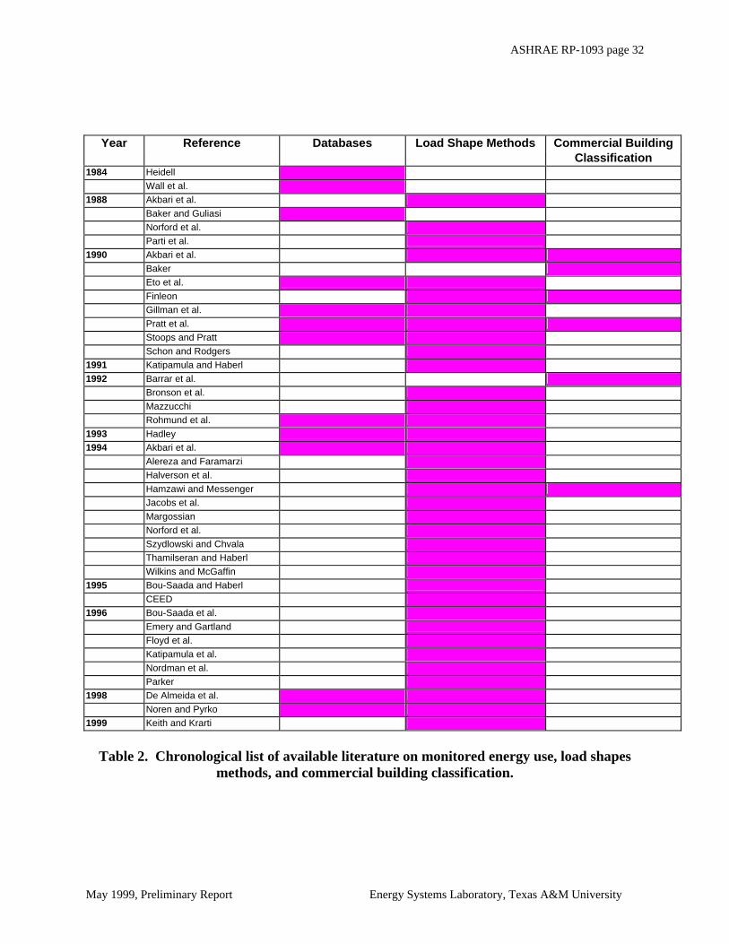
ASHRAE RP-1093 page 32
May 1999, Preliminary Report Energy Systems Laboratory, Texas A&M University
Year Reference Databases Load Shape Methods Commercial Building
Classification 1984 Heidell Wall et al. 1988 Akbari et al. Baker and Guliasi Norford et al. Parti et al. 1990 Akbari et al. Baker Eto et al. Finleon Gillman et al. Pratt et al. Stoops and Pratt Schon and Rodgers 1991 Katipamula and Haberl 1992 Barrar et al. Bronson et al. Mazzucchi Rohmund et al. 1993 Hadley 1994 Akbari et al. Alereza and Faramarzi Halverson et al. Hamzawi and Messenger Jacobs et al. Margossian Norford et al. Szydlowski and Chvala Thamilseran and Haberl Wilkins and McGaffin 1995 Bou-Saada and Haberl CEED 1996 Bou-Saada et al. Emery and Gartland Floyd et al. Katipamula et al. Nordman et al. Parker 1998 De Almeida et al. Noren and Pyrko 1999 Keith and Krarti
Table 2. Chronological list of available literature on monitored energy use, load shapes
methods, and commercial building classification.

ASHRAE RP-1093 page 33
May 1999, Preliminary Report Energy Systems Laboratory, Texas A&M University
Method's Name Nature* Basis** Weather-dependent
Weather-independent
Reference
Stephan-Demming Algorithm Deterministic Engineering/Monitoring
X X (SRC 1988, ref. Eto et al.1990)
End-use Disaggregration Algorithm (EDA)
Deterministic Engineering/Monitoring
X X (Akbari et al. 1988)
Conditional Energy Demand (CED)
Statistical Monitoring X X (Parti et al. 1988)
Variance Allocation Deterministic Engineering/Monitoring
X X (Schon and Rodgers 1990)
Bi-level Regression Statistical Engineering/Monitoring
X X (SSI 1986, ref. Eto et al. 1990)
Statistically Adjusted Engineering approach (SAE)
Statistical Engineering/Monitoring
X X (CSI, CA, ADM 1985, ref. Eto et al. 1990)
Mean / Standard Deviation / Regulatory Index
Statistical Engineering/Monitoring
X (Katipamula and Haberl 1991)
Temporal Synoptic Index (TSI) Statistical Monitoring X (Hadley 1993) Heuristic Pattern Recognition Algorithm
Deterministic Monitoring X X (Margossian 1994)
Inverse Binning Method Statistical Monitoring X (Thamilseran and Haberl 1994)
Temperature-binning Daytyping Statistical Monitoring X (Bou-Saada and Haberl 1995), (Noren and Pyrko 1998)
Pattern Group Assignment Statistical Monitoring X X (Emery and Gartland 1996)
* Deterministic Methods: Methods that rely on exact reconciliation to an hourly control total, which is provided by the hourly whole-building load research data. The starting point for the reconciliation is an engineering simulation of the sort relied upon by the earliest load shape estimation methods. The methods typically rely on much more detailed information to develop the simulation input (minimizing the extensive reliance on engineering judgement) (Eto et al. 1990). Statistical Methods: Methods that typically rely on regression techniques that correlate explanatory variables with the hourly control total. These variables need not all be physical and the reconciliation to the control total is usually expressed in goodness of fit.
** Engineering methods: Methods based on pure simulations of whole-building energy use and/or different end-uses. Monitoring Methods: Methods that involve monitored whole-building energy use.
Note: Simple average and standard deviation deterministic methods, based on metered end-uses, are not included in this table. Only methods that disaggregate whole-building energy use to derive typical load shapes for end-uses are listed, besides some other sophisticated approaches.
Table 3. Existing methods for daytyping and determining load shapes of end-uses.
Table 3 shows that the first Deterministic method used for deriving load shapes was the
Stephan-Deming Algorithm (1988), which is a statistical adjustment procedure in which elements of an end-use matrix are adjusted when the terminal values, for instance total hourly load, are known. When only the hourly whole-building load is known, a weighted distribution of the difference between the measured total and the sum of the simulated end-uses, based on the magnitude of the original simulated estimates, is applied.
The second Deterministic method was the Energy-use Disaggregation Algorithm (EDA)
(1988) which is an engineering method that primarily utilizes the statistical characteristics of the measured hourly whole-building load and its statistical dependence on temperature. In the EDA the sum of the end uses is constrained at hourly intervals to be equal to the measured whole-building load, providing a reality check not always possible with pure simulation. The intent of the method is to supply reasonable end-use breakdowns when detailed information is scarce.

ASHRAE RP-1093 page 34
May 1999, Preliminary Report Energy Systems Laboratory, Texas A&M University
This method is a hybrid method that uses monitored data, statistical disaggregation, and prorating based on a simulation.
The third Deterministic method is the Variance Allocation method (1990) which is a hybrid engineering/ statistical approach to end-use load shape estimation for the commercial sector. The method (1) identifies systematic biases in engineering model hourly end-use load estimates, (2) adjusts the engineering model to significantly reduce these biases for individual building end-use estimates, and (3) uses a variance-weighted approach to reconcile adjusted engineering estimates with whole-building metered data. To reconcile the sum of the hourly end-use load estimates with each individual facility's hourly research data, the variances observed for each regression coefficient are used. The difference between simulated and metered totals is prorated based on statistical variation in the simulated end-use loads. The largest and most variant end-uses receive the largest portion of the difference between the engineering simulation and the metered whole-building load.
The fourth Deterministic method is the Heuristic Pattern Recognition Algorithm (1994)
which is used to disaggregate premise-level load profiles. This algorithm uses as input 5-minute or 15-minute residential premise-level load data; it also requires as input connected load estimates of the cooling, heating and water heating appliances. The algorithm first scans the premise-level load profile and identifies all spikes in the profile that are large enough with respect to the connected load of the space conditioning appliance, and categorizes these spikes with various attributes such as shape, timing, magnitude, and duration. In a second stage, the classification stage, the algorithm decides whether or not to attribute each of the identified spikes to the space conditioning appliance. The resulting spikes comprise the end-use load profile for the space conditioning appliance on that day. The load profile of the water heating appliance is derived from the residuals of the premise-level load profile, after subtracting the space conditioning appliance load profile, using the scanning and classification stages.
The first Statistical method is the Conditional Energy Demand (CED) technique (1988). In this technique the end-use metered consumption information are used only for comparison to the CED estimates of end-use load shapes. The CED carries out the disaggregation of the total load into its end-use components by applying Multiple Linear Regression (MLR) analysis to a data set composed of total load data, survey and weather information. The model breaks down the hours of the day into four general hourly categories: (1) Night, (2) Morning, (3) Midday, and (4) Evening.
The second Statistical method is the Statistically Adjusted Engineering approach (SAE)
(1985) which is very close to the Deterministic methods. First an engineering simulation is developed to provide an initial estimate of end-use loads. Next, the initial estimates are regressed against control totals, which are averages of hourly energy use for typical days. The estimated coefficients can then be thought of as adjustment factors that reconcile the initial estimates to the control total.
The third Statistical method is the Bi-level Regression approach (1986) which involves
two levels of time series and cross section regression analyses. In the first level, the hourly load of individual households is regressed against both weather-related variables, and sine and cosine functions which capture daily, weekly, and seasonal periodicity in loads that are independent of
ASHRAE RP-1093 page 35
May 1999, Preliminary Report Energy Systems Laboratory, Texas A&M University
weather. In the second level, the coefficients estimated in the first level (separately for each household) are regressed as a group against customer characteristics.
The fourth Statistical method is the Mean/Standard Deviation/Regulatory Index method
(1991). The method identifies typical daytypes for a building, using monitored non-weather-dependent electricity use. Load shapes are generated from the data for each typical daytype. In deriving the daytypes, the mean and the standard deviation of the energy use at each hour for the entire data group were calculated, and a Regularity Index (RI) is calculated and checked against a maximum acceptable value (10%) for each hour. If the RI for all 24 hours exceeds the 10% value, hourly data is summed to daily totals and the mean and standard deviation of the daily consumption are calculated. Three daytypes are then identified as follows: (1) LOW-D days with daily consumption lower than Y (10%) times one standard deviation below the mean; (2) HIGH-D days with daily consumption higher than Y times one standard deviation above the mean; and (3) NORMAL-D , the remaining days. The daytypes are then subdivided to LOW-LOW D, LOW-HIGH D, LOW-NORMAL D, HIGH-LOW D, HIGH-HIGH D, HIGH-NORMAL D, NORMAL-D, NORMAL-LOW D, AND NORMAL-HIGH D.
The fifth Statistical method is the Temporal Synoptic Index approach (TSI) (1993) for weather-dependent data which uses a combination of principal component analysis (PCA) and cluster analysis on the resultant principal components (PC’s), to identify days which are considered meteorologically homogeneous. Once the number of daytypes is specified, each day in the data set analyzed can be assigned to a specific, unique daytype and the average values of each meteorological variable calculated for each daytype. Each weather-daytype is defined in terms of the daily average of the dry-bulb and wet-bulb temperature, extraterrestrial and total global horizontal radiation, clearness index, and wind speed. The unique character of each weather daytype is established by: (1) the mean value of each of the original weather variables within each daytype; (2) the frequency of occurrence of the daytype by month; and (3) the diurnal variation of each variable within each daytype. The statistical techniques followed in this method might be helpful in deriving weather-independent load shapes.
The sixth Statistical method is the Inverse Binning approach (1994) for non-weather-
dependent loads. The general pattern of the energy use is identified graphically to show the effect of weekdays-weekends and holidays and the periodicity of the peak consumption. Then the Pearson’s correlation technique is used to identify the correlation between dependent and independent variables. The “hour of the day” is used as a bin variable in the non-weather-dependent loads model. Duncan’s, Duncan-Waller’s and Scheffe’s multiple comparison tests are used to aggregate the data into daytypes that have means with statistically insignificant differences. The technique includes the following steps: (1) identification of general patterns of data (from database), (2) checking for temperature dependency of Hour of the Day (HOD) dependency, (3) checking for data quality and outliers identification, (4) identification of comprehensive daytypes, (5) checking for impact of ON/OFF mode, (6) calculation of binned energy, (7) correction for missing bins, (8) checking for need for thermal lag, (9) checking for need for humidity sub-binning, (10) final calculation of binned energy and correction for missing bins.
ASHRAE RP-1093 page 36
May 1999, Preliminary Report Energy Systems Laboratory, Texas A&M University
The seventh Statistical method is the Tempearture-binning Daytyping technique (1995 and 1998). Bou-Saada and Haberl (1995) categorized the whole-building electricity consumption of an electrically heated-cooled building into three weather-daytypes (below 45oF, between 45 oF and 75oF, and above 75oF). An average heating profile was chosen to represent all hours when temperatures were below 45 oF, an average cooling profile was selected for temperatures above 75 oF, while non-HVAC profile was assigned for all hours between a temperature of 45 oF and 75
oF. For the non-HVAC profile, two representative days, weekday and weekend days, were chosen by visual inspection of the data. Disaggregation of the non-weather-dependent electric load was then performed by reviewing site plans, hand measurements during site visits and personal interviews. In a similar way, Noren and Pyrko (1998) presented load shapes developed for different mean daily outdoor temperatures and different daytypes; standard weekdays and standard weekends. The load shapes are presented as non-dimensional normalized 1-hour loads. The methodology consisted of calculating the normalized load by dividing the measured load at time t by the mean annual load. Then the data are split into different groups, depending on the daytype. The data in every group are sorted by hour, and every hour sorted into different temperature intervals. Six different integrals for mean daily outdoor temperature were used to sort the data. A mean normalized value of the load can be calculated for every hour and each temperature interval, by dividing the calculated normalized load by the total number of observations at time t for a category at specified temperature interval. The statistical techniques used in these two methods can prove helpful in deriving the diversity factors for this project.
Finally, the eighth Statistical method is the Pattern Group Assignment (1996) which
groups together days with common behavioral load shapes or patterns, instead of grouping energy behaviors together based on the day of the week, as in daytyping algorithms. Pattern codes are assigned in reference to the frequency distribution of a certain behavior. With this technique, there is flexibility in the level of detail available to the pattern code. Different numbers of sections, and different numbers and designations of time periods can be chosen depending on the data and the level of accuracy needed. Once the pattern codes are assigned to each day, the days are iteratively assigned to groups. In the first iteration, days with the same pattern code are grouped together. In the second and proceeding iterations, groups with similar pattern codes and the lowest combination errors are combined until there are no more groups with sufficiently similar pattern group codes.
Our review of the literature has indicated that there are several useful studies that present
actual diversity factors, and provide the algorithms or procedures for deriving the diversity factors. This extensive literature review will provide us with a useful set of load shapes tools and methods for deriving diversity factors from end-use and whole-building electricity data.
We propose to test these methods against the Predictor Shootout I (Kreider and Haberl
1994) and Predictor Shootout II (Haberl and Thamilseran 1996) data sets which were used by contestants from within and outside the U.S. to test different energy use prediction methods. The results of this test will be reported in the report of Phase 2 of this project.

ASHRAE RP-1093 page 37
May 1999, Preliminary Report Energy Systems Laboratory, Texas A&M University
2.2 ANNOTATED BIBLIOGRAPHY Akbari, H., J. Eto, S. Konopacki, K. Heinemeier, and L. Rainer. 1994. A new approach to estimate commercial sector end-use load shapes and energy use intensities. Proceedings of the 1994 ACEEE Summer Study on Energy Efficiency in Buildings, pp. 2.2-2.10. This paper describes an end-use load shape estimation technique to develop annual energy use intensities (EUI’s) and hourly end-use load shapes (LS’s) for commercial buildings in the Pacific Gas and Electric company (PG&E) service territory. The results were ready to use as inputs for the commercial sector energy and peak demand forecasting models used by PG&E and California Energy Commission (CEC). The initial end-use load shape estimates were developed with DOE-2 using building prototypes based on surveys. Then average measured whole-building load shapes and annual energy use intensities were derived. The initial end-use load shapes were reconciled with the measured whole building load shape data, by applying the End-use Disaggregation Algorithm (EDA) to obtain reconciled end-use LS’s and corresponding EUI’s. Akbari, H., Heinemeier, K., Le Coniac, P., and Flora, D. 1988. An algorithm to disaggregate commercial whole-building electric hourly load into end-uses. Proceedings of the 1988 ACEEE Summer Study on Energy Efficiency in Buildings, pp. 10.13-10.36. This paper describes an Energy-use Disaggregation Algorithm (EDA), an engineering method which primarily utilizes the statistical characteristics of the measured hourly whole-building load and its inferred dependence on temperature. The primary component of the EDA is the regression of hourly load with outdoor dry bulb temperature. Two season-specific (summer and winter sets of temperature regression coefficients are used to cover the temperature dependency of the building load. Twenty-four regression models (for each hour) are developed for each season. The temperature regression equations are used to separate the load predicted by the regression, LREG, into a temperature-dependent part, LTD, and a temperature-independent part, LTI. The temperature-independent load is then prorated according to the loads predicted by a simulation developed based on a building audit. Akbari, H., Turiel, I., Eto, J., Heinemeier, K., and Lebot, B. 1990. A review of existing commercial energy use intensity and load shapes studies. Proceedings of the 1990 ACEEE Summer Study on Energy Efficiency in Buildings, pp. 3.7-3.18. This paper reviews and compares existing studies of energy use intensities (EUI) and load shapes (LS) in the commercial sector, focusing on studies that used California data. The study uncovered two significant features of existing LS estimates. First, the LS's were generally not consistent between studies (for the same end-use in the same type of premises), but these differences could often be related to differences in assumptions for operating hours. Second, for a given type of premises, the LS's were often identical for each month and for peak and standard days, suggesting that, according to some studies, these end-uses were not affected by seasonal or climatic influences.
Alereza, T., and Faramarzi, R., 1994. More data is better, but how much is enough for impact evaluations? Proceedings of the 1994 ACEEE Summer Study on Energy Efficiency in Buildings, pp. 2.11-2.19.

ASHRAE RP-1093 page 38
May 1999, Preliminary Report Energy Systems Laboratory, Texas A&M University
This paper evaluates how well energy use predicted with building energy simulation models compares with energy use measured by end-use metered data, and demonstrates how predicted energy use is affected by different levels of data availability. The following levels of resolution were defined: (1) detailed building characteristics data collected on-site, (2) monthly energy and peak demand billing information with level (1) data, (3) inspection of working condition of HVAC equipment with level (2) data, (4) measured whole building hourly data with level (3) data, and (5) monitored end-use data for major non-conditioning loads with level (4) data. Load shapes for each step were developed to illustrate the improvement in the general accuracy. In progressing from Level 1 to Level 5 load estimation procedures, the average error observed for whole building consumption was cut by 77%, with the greatest gains coming from billing data and lighting monitoring data. ASHRAE 1989. ASHRAE Standard 90.1. Energy Efficient Design of New Buildings Except Low-Rise Residential Buildings. American Society of Heating, Refrigeration and Air-Conditioning Engineers, Atlanta, Georgia. This ASHRAE Standard lists diversity factors obtained from a study conducted at Pacific Northwest Laboratory. The compiled table includes diversity factors for: (1) Occupancy, (2) Lighting and Receptacles, (3) HVAC, and (4) Service Water Heating (SWH). Three load shapes (Weekday, Saturday, Sunday) were included for each of the following categories: (1) Assembly, (2) Office, (3) Retail, (4) Warehouse, (5) School, (6) Hotel/Motel, (7) Restaurant, (8) Health, and (9) Multi-Family. ASHRAE 1991. ASHRAE Handbook of HVAC Applications. American Society of Heating, Refrigeration and Air-Conditioning Engineers, Atlanta, Georgia. This ASHAR Handbook displays load shapes for general categories for buildings, for instance, office buildings and warehouses. The load profile of the Office buildings is shown to peak at 4:00 PM. That of the warehouse peaks at 10:00 AM to 3:00 PM. Baker, M. 1990. Utility application of commercial sector end-use load measurements: Case studies are not good enough!. Proceedings of the 1990 ACEEE Summer Study on Energy Efficiency in Buildings, pp. 3.27-3.34. This paper describes guidelines for designing an effective integrated approach to end-use research, and presents a sample application based on commercial customer data collected in the Pacific Northwest. The paper emphasizes the importance of specifying the appropriate objective for end-use metering by focusing on only the most important market segments. It categorizes the commercial sector by the following major, relatively homogeneous market segments: (1) Office, (2) Dry Goods Retail, (3) Grocery, (4) Restaurant, (5) Warehouse, and (6) Education. The rest of the commercial sector comprises minor segments that are nearly impossible to classify. Baker, M. and Guliasi, L. 1988. Alternative approaches to end-use metering in the commercial sector: The design of Pacific Gas and Electric Company's commercial end-use metering project. Proceedings of the 1988 ACEEE Summer Study on Energy Efficiency in Buildings, pp. 10.28-10.41. This paper describes the design of a commercial end-use metering study for Pacific Gas and Electric Company (PG&E) and examines other metering studies conducted earlier. It states that commercial end-use metering studies were conducted for two analytic purposes: (1) building
ASHRAE RP-1093 page 39
May 1999, Preliminary Report Energy Systems Laboratory, Texas A&M University
energy performance analysis, and (2) class load end-use analysis. Class load end-use studies are usually intended to support the estimation of end-use share, end-use intensity, and load shape (diurnal and seasonal) for the following types of building activities: (1) long-run energy and peak demand forecasts, (2) conservation and load management program assessments, (3) marketing assessments, (4) capacity planning for transmission and distribution, and (5) cost-of-service/rate design. Three distinct models of measurements for class load end-use studies are usually used: (1) detailed end-use measurements, (2) summary end-use measurements, and (3) equipment load survey. Barrar, J., Ellison, D., Wikler, G., and Hamzawi, E. 1992. Integrating engineering-based modeling into commercial-sector DSM program planning. Proceedings of the 1992 ACEEE Summer Study on Energy Efficiency in Buildings, pp. 3.23-3.32. This paper describes a building prototype technique that estimates the DSM resource potential within the Potomac Electric Power Company (Pepco) commercial sector. A six-step process was developed: (1) define baseline conditions to develop metered baseline load shapes, (2) run baseline simulations to develop simulated baseline load shapes, (3) develop DSM measure scenarios, (4) re-run simulations with DSM measures, (5) bundle passing measures into DSM programs, and (6) re-run simulations with DSM programs. The following building types were selected for the prototype analysis: (1) Large Private Offices, (2) Large Government Offices, (3) Large Hospitals, (4) Large Hotels, and (5) Master-metered Apartments (all sizes). Bou-Saada, T.E., Haberl, J.S., Vajda, E.J., Shincovich, M., D'Angelo, L., and Harris, L. 1996. Total utility savings from the 37,000 fixture lighting retrofit to the U.S. DOE Forrestal Building. Proceedings of the 1996 ACEEE Summer Study on Energy Efficiency in Buildings, pp. 4.31-4.48. This paper provides an overview of the lighting retrofit and the resultant electricity and thermal savings at the DOE Forrestal Building. The methodology that has been applied to calculate the gross, whole-building electricity, and thermal savings from the lighting retrofit uses a before-after analysis of the whole-building electricity and thermal use. The methodology separately calculates weather-dependent and weather-independent energy use by developing empirical baseline models that are consistent with the known loads on a given channel. Bou-Saada, T.E., and J.S. Haberl. 1995. A weather-daytyping procedure for disaggregating hourly end-use loads in an electrically heated and cooled building from whole-building hourly data. Proceedings of the 30th Intersociety Energy Conversion Engineering Conference, July 31-August 4 1995, Orlando, FL, pp. 323-330. This paper presents a weather daytyping procedure capable of disaggregating whole-building electricity signal into end-use loads. Representative days were used to designate the non-weather dependent base load for occupied and non-occupied hours which were then sorted into three additional weather types: one for cooling, one for heating and one for non-heating/non-cooling. Results of applying this methodology to a case study building in Washington, D.C. were also presented. Bronson, D.J., S. Hinshey, J.S. Haberl, and D.L. O’Neal. 1992. A procedure for calibrating the DOE-2 simulation program to non-weather-dependent measured loads. ASHRAE Transactions 98 (1).

ASHRAE RP-1093 page 40
May 1999, Preliminary Report Energy Systems Laboratory, Texas A&M University
This paper describes a procedure to calibrate DOE-2 building simulation program to non-weather dependent (or scheduled) loads. The procedure relies on special purpose 3-D graphics of differences in hourly monitored and simulated data as an aid in the calibration process. Four different methods of daytyping routines were used to demonstrate the effectiveness of the procedure. The study showed that the results using DOE-2 daytype profiles were outperformed by the results of all other methods when the simulated data was compared against the monitored data. CEED 1995. Leveraging limited data resources: Developing commercial end-use information: BC Hydro case study. Technical Report. EPRI's Center for Electric End-Use Data (CEED). Portland, Oregon. This report provides the results of a collaborative research project with BC Hydro where model-based sampling, building total load research data, audits, DOE-2.1 models, and borrowed end-use data were combined to produce statistically reliable end-use information for the commercial office sector. The study demonstrated that end-use data can be developed in shorter time, at less expense, with statistically reliable results than more conventional approaches.
De Almeida, A.T., Saraiva, N., Roturier, J., Anglade, A., and Jensen, M. 1998. Management of the electricity consumption in the office equipment end-use for an improved knowledge of usage in the tertiary sector in Europe. Proceedings of the 1998 ACEEE Summer Study on Energy Efficiency in Buildings, pp. 5.35-5.47. This European paper reports a large field measurement campaign, MACEBUR, that was carried on in three European countries to assess the power load and electricity consumption of energy efficient (Energy Star, E*) office equipment in office buildings. More than 2000 units were metered in total. The Danish case study was carried on in four different locations in Denmark. The French case study included eight different French locations. Data from about 600 machines were analyzed. The third case study was conducted in Portugal, and the results, in terms of hours of usage per day, were similar to the French results. The campaign found that in Denmark where the building standards are very stringent, building managers are very aware of the internal gains, since they increase the indoor air temperature, and thus lower the employee's productivity. Also, E* is not commonly known and energy management is better performed through a manual turn-off by the user. In France and Portugal, energy policies are not in priority oriented towards energy efficiency. The result is that there is little concern with the electricity end-use sector. Emery, A.F., and Gartland, L.M. 1996. Quantifying occupant energy behavior using pattern analysis techniques. Proceedings of the 1996 ACEEE Summer Study on Energy Efficiency in Buildings, pp. 8.47-8.59. This paper describes analysis techniques developed to extract behavioral information from collected residential end-use data. Four statistical methods have been tested and found useful in their study of energy behavior: (1) daily time-series averages and standard deviations, (2) frequency distributions, (3) assignment of days to pattern groups, and (4) multinomial logit analysis to examine pattern group choice. The four techniques were tested successfully using end-use data for families living in four heavily instrumented residences in a University of Washington project. A new algorithm, the Pattern Group Assignment, described in this paper, was developed to group together days with common behavioral load shapes or patterns, instead of grouping energy behaviors together based on the day of the week, as in daytyping algorithms.

ASHRAE RP-1093 page 41
May 1999, Preliminary Report Energy Systems Laboratory, Texas A&M University
The pattern analysis and multinomial logit model were able to match the occupant behavior correctly 40 to 70% of the time. The steadier behaviors of indoor temperature and ventilation were matched most successfully. EPRI 1999. EPRI's Southeast Data Exchange. Information obtained from EPRI-CEED website. Center for Electric End-Use Data (CEED). Portland, Oregon. This information from the EPRI website reports developing load shapes and new tools that can be fed directly into the EPRI's ProfitManager model and other software, helping participants jump-start efforts to produce accurate load estimates for a host of retail marketing application. Nine Southwestern utilities approached EPRI's CEED (Center for Electric End-Use Data) to develop methods and models to transfer the data to their service areas. A library of load shapes was obtained as a result of the study. Eto, J.H., Akbari, H., Pratt, R., and Braithwait, S. 1990. End-use load shape data: Application, estimation, and collection. Proceedings of the 1990 ACEEE Summer Study on Energy Efficiency in Buildings, pp. 10.39-10.55. This paper identifies 27 end-use metering projects in the U.S., eleven of which are in the commercial building sector and discusses the importance of end-use load shape data for utility integrated resource planning, and summarized leading utility applications and reviewed latest progress in obtaining load shape data. The paper described six different methods used in load shape estimation: (1) one dimension application of the Stephan-Deming Algorithm, (2) the variance allocation approach, (3) the End-use Disaggregation Algorithm (EDA), (4) the Conditional Demand Approach, (5) the bi-level regression approach, and (6) the Statistically Adjusted Engineering approach (SAE). Finleon, J. 1990. A method for developing end-use load shapes without end-use metering. Proceedings of the 1990 ACEEE Summer Study on Energy Efficiency in Buildings, pp. 10.57-10.65. This paper describes a methodology whereby end-use load shapes for residential and commercial/industrial buildings can be developed without undertaking a new end-use metering project. In the residential sectors load shapes were developed for the following end-uses: (1) electric heating, (2) refrigerators, (3) electric dryers, (4) electric water heating, (5) air conditioning, (6) freezers, (7) cooking, and (8) other. In this sector, load shapes were developed for the following end-uses: (1) Electric heating, (2) lighting, (3) refrigeration, (4) air conditioning, (5) water heating, and (6) other. Floyd, D.B., Parker, D.S., and Sherwin, J.R. 1996. Measured field performance and energy savings of occupancy sensors: Three case studies. Proceedings of the 1996 ACEEE Summer Study on Energy Efficiency in Buildings, pp. 4.97-4.105. This paper reports two studies conducted in Florida on the use of occupancy sensors. In an effort to measure performance, energy savings, and occupant acceptance, occupancy sensors were installed in a small office building and two elementary schools. 15-minute data were collected to assess performance. Aggregate time-of-day lighting load profiles are compared before and after the installation and throughout the commissioning period when the sensors are tuned for optimum performance. Savings of 10% to 19% in small office and 11% in school were reported in this paper.

ASHRAE RP-1093 page 42
May 1999, Preliminary Report Energy Systems Laboratory, Texas A&M University
Gillman, R., Sands, R.D., and Robert, G.L. 1990. Observations on residential and commercial load shapes during a cold snap. Proceedings of the 1990 ACEEE Summer Study on Energy Efficiency in Buildings, pp. 10.81-10.89. This paper reports on the End-use Load and Consumer Assessment Program (ELCAP) which collected hourly metered and associated characteristics data for approximately 400 residential and commercial buildings equipped to meter hourly electricity consumption for up to 16 end-uses in residences, and 20 end-uses in commercial buildings. Average load shapes were created, in the ELCAP study, for each building type and end-use by averaging hourly electricity consumption data across sites. Haberl, J.S., and P. Komor. 1989. Investigating an analytical basis for improving commercial building energy audits: Results from a New Jersey mall. Center for Energy and Environmental Studies Report No. 264, June 1989. This research report at Princeton University includes the detailed procedures followed to improve energy audits. Specifically, the report describes a method to synthesize square profiles to predict the load profiles for lights and receptacles data, without performing hourly monitoring. Haberl and Komor (1990a, and b) are based on this report. Haberl, J.S., and P. Komor. 1990a. Improving commercial building energy audits: How annual and monthly consumption data can help. ASHRAE Journal (August). This paper describes an energy audit study of a shopping center, that adopts an approach recommended by ASHRAE. The approach recommends that a commercial building energy analysis be performed interactively using three levels: (1) an analysis of past utility information, (2) a simple walk-through and brief analysis, and (3) a detailed engineering analysis. Calculated indices such as the Monthly Electric Load Factors (ELF), and the Monthly Occupancy Load Factors (OLF), were used among other indices. Comparing the ELF and the OLF for same periods of time confirmed that equipment or lights were left operating during unoccupied periods, and disparity in peak electric demand and usage occurred during the fall. Haberl, J.S., and P. Komor. 1990b. Improving commercial building energy audits: How daily and hourly consumption data can help. ASHRAE Journal (August). This paper reports the daily and hourly results of the study conducted on the shopping center described in (Haberl and Komor 1990.a). Daily and hourly presentation of the metered energy consumption were considered to discover what could be learned about each site and whether preliminary indications were present in the indices that suggested possible energy conservation measures. Haberl, J.S., and Thamilseran, S, 1996. The Great Energy Predictor Shootout II: Measuring retrofit savings - Overview and discussion. ASHRAE Transaction 1996, V. 102, Pt. 2. This paper summarizes the comparative prediction accuracy of several models of hourly building energy use data. This second shootout competition, open to anyone who wished to participate, involved the following steps: (1) each contestant was supplied with identical baseline data set consisting of hourly energy use data and climatic variables for a certain period of the year for two buildings, (2) the contestants then developed models (regression, artificial neural networks, etc.) based on this baseline data, and (3) the judges then used these models to predict energy use
ASHRAE RP-1093 page 43
May 1999, Preliminary Report Energy Systems Laboratory, Texas A&M University
into the future for which they alone had monitored data, and ranked the entries based on their predictive accuracy. Hadley, D.L. 1993. Daily variations in HVAC system electrical energy consumption in response to different weather conditions. Energy and Buildings, V.19 (1993), pp. 235-247. This paper describes a very sophisticated weather-daytyping routine that may prove useful for application for deriving diversity factors from whole-building loads. A Temporal Synoptic Index (TSI) approach is developed, which uses a combination of principal component analysis (PCA) and cluster analysis on the resultant principal components (PC’s), to identify days which are considered meteorologically homogeneous. Once the number of daytypes is specified, each day in the data set analyzed can be assigned to a specific, unique daytype and the average values of each meteorological variable calculated for each daytype. The unique character of each weather daytype was established by: (1) the mean value of each of the original weather variables within each daytype; (2) the frequency of occurrence of the daytype by month; and (3) the diurnal variation of each variable within each daytype. Halverson, M.A., Stoops, J.L., Schmelzer, J.R., Chvala, W.D., Keller, J.M., and Harris, L.R. 1994. Lighting retrofit monitoring for the federal sector - Strategies and results at the DOE Forrestal Building. Proceedings of the 1994 ACEEE Summer Study on Energy Efficiency in Buildings, pp. 2.137-2.144. This paper describes a short-term monitoring strategy in a study conducted at the DOE Forrestal Building to: (1) assist in the development of the Shared Energy Savings (SES) request for proposal (RFP) from potential lighting retrofit contractors, and (2) provide empirical data that could be used to confirm predicted results. Three distinct but integrated monitoring activities were planned: (1) baseline monitoring of the existing lighting loads, (2) performance monitoring of any proposed lighting retrofit, and (3) post-retrofit monitoring of the new lighting loads. The results of the baseline monitoring were detailed weekday and weekend end-use profiles of the Forrestal electrical consumption. The developed lighting load profile showed that a large amount of lighting occurs 24 hours a day. Post-retrofit monitoring also resulted in weekday and weekend profiles, that showed savings of 55.4% and 57.4% in daily consumption respectively. Hamzawi, E. H., and Messenger, M., 1994. Energy and peak demand impact estimates for DSM technologies in the residential and commercial sectors for California: Technical and regulatory perspectives. Proceedings of the 1994 ACEEE Summer Study on Energy Efficiency in Buildings, pp. 2.145-2.155. This paper describes estimates of energy savings and peak demand impacts from the implementation of a host of DSM technologies in 16 commercial and two residential building types. The overall approach employed involved collecting data for establishing baseline residential Unit Energy Consumption (UEC), commercial Energy Utilization Intensity (EUI), and average load shape information and base case residential and commercial building prototypes, simulating energy use from the base case prototypes, and reconciling the results with the baseline UEC and EUI, and load shape data, to estimate the energy savings, coincident peak demand impacts, and load shapes associated with conservation measures.

ASHRAE RP-1093 page 44
May 1999, Preliminary Report Energy Systems Laboratory, Texas A&M University
Heidell, J.A. 1984. Development of a data base on end-use energy consumption in commercial buildings. Proceedings of the 1984 ACEEE Summer Study on Energy Efficiency in Buildings, pp. D-49 - D-62. This paper reports on a comprehensive inventory database of end-use metered data in commercial buildings, conducted by Battelle - Pacific Northwest Laboratory. The inventory was prepared in order to develop an assessment of end-use data on existing commercial buildings and to determine the need for a public domain database. The inventory included 55 metering projects, along with the corresponding building types, location, data type, time resolution, metering technique, and availability of the data (public or private domain). Jacobs, P.C., Waterbury, S.S., Frey, D.J., and Johnson, K.F. 1994. Short-term measurements to support impact evaluation of commercial lighting programs. Proceedings of the 1994 ACEEE Summer Study on Energy Efficiency in Buildings, pp. 5.113-5.121. This paper describes surrogate measurements techniques used to reduce the costs associated with true power measurements. Specialized data loggers were used to monitor some easily observed parameters such as fixture on/off status, fixture light output, or lighting circuit current. This information combined with measurements of lighting fixture power was used to estimate energy consumption and savings resulting from lighting measures. In one case study, the estimates of average workday energy consumption from surrogate measurements varied from the true power measurements by 4%, while the estimates of average workday peak demand varied from the true power measurements by about 30%. Katipamula, S., Allen, T., Hernandez, G., Piette, M.A., and Pratt, R.G. 1996. Energy savings from Energy Star personal computer systems. Proceedings of the 1996 ACEEE Summer Study on Energy Efficiency in Buildings, pp. 4.211-4.218. This paper reports on a metering study that was conducted at a typical single-story commercial building located in Northern California, in order to quantify the energy savings potential of Energy Star-compliant PCs. The energy consumption of the monitor and the central processing unit (CPU) for the ES-compliant PCs was monitored in 15-minute time series records to emulate the utility billing demand interval. The potential energy savings were computed by comparing the average 24-hour demand profile of an ES-compliant PC to that of standard PC. The savings at the office building represented 59% in PC systems energy consumption. Katipamula, S., and J.S. Haberl. 1991. A methodology to identify diurnal load shapes for non-weather dependent electric end-uses. Proceedings of the 1991 ASME-JSES International Solar Energy Conference, New York, N.Y., pp. 457-467. This paper reports the identification of typical daytypes for a building, using monitored non-weather-dependent electricity use. Load shapes were generated from the data for each typical daytype and used as schedules in a DOE-2 building energy simulation model. In deriving the daytypes, the mean and the standard deviation of the energy use at each hour for the entire data group were calculate, and a Regularity Index (RI) was calculated and checked against a maximum acceptable value (10%) for each hour. If the RI for all 24 hours exceeds the 10% value, hourly data is summed to daily totals and the mean and standard deviation of the daily consumption are calculated. Three daytypes are then identified. The daytypes are finally subdivided to LOW-LOW D, LOW-HIGH D, LOW-NORMAL D, HIGH-LOW D, HIGH-HIGH

ASHRAE RP-1093 page 45
May 1999, Preliminary Report Energy Systems Laboratory, Texas A&M University
D, HIGH-NORMAL D, NORMAL-D, NORMAL-LOW D, AND NORMAL-HIGH D. As a result, the hourly load average profile for each daytype was generated. Keith, D.M., and Krarti, M. 1999. Simplified prediction tool for peak occupancy rate in office buildings. Journal of the Illuminating Engineering Society, Winter 1999, pp. 43-52. This paper summarizes a methodology used to develop a simplified prediction tool to estimate peak occupancy rate from readily available information, specifically average occupancy rate and number of rooms within an office building. The study was carried on in a laboratory campus with three similar two and three story buildings in Boulder, CO, comprising approximately 1200 rooms, with 1174 having individual occupancy sensors. Calculations include every 5 minutes period within the daily period of interest over the month, counting the occupied and unoccupied records for all the rooms in the specified set. To determine the peak occupancy rate, numerous combinations of linear terms were evaluated, starting with just the two independent variables of average occupancy rate and number of rooms, and increasing the number and variety of terms to develop the best fit. A multiple linear regression model of peak occupancy rate was finally developed which is function of average occupancy rate, number of rooms, and other variables which are combinations of these two variables. Komor, P. 1997. Space cooling demands from office plug loads. ASHRAE Journal (December). This paper reports on a study conducted using nameplate ratings of office equipment data drawn from 44 typical office buildings of 1.3 million ft2 total floor area, to show that ratings are not intended for use in calculating actual non-instantaneous power use or heat output. The study notes the importance of using diversity factors and shows that actual plug loads ranged from 0.4 to 1.1 W/ft2, which is considerably lower than the 4.4 W/ft2 noted by the 1993 ASHRAE Fundamentals Handbook. The study provides useful snapshot indices of office equipment. Kreider, J.F., and Haberl, J.S. 1994. Predicting hourly building energy use: The Great Energy Predictor Shootout - Overview and discussion of results. ASHRAE Transactions 1994, V.100, Pt. 2. This paper summarizes the comparative prediction accuracy of several models of hourly building energy use data based on limited amounts of measured data. This first shootout competition, open to anyone who wished to participate, involved the following steps: (1) each contestant was supplied with identical baseline data set consisting of hourly energy use data and climatic variables for a certain period of the year for two buildings, (2) the contestants then developed models (regression, artificial neural networks, etc.) based on this baseline data. Margossian, B. 1994. Deriving end-use load profiles without end-use metering: Results of recent validation studies. Proceedings of the 1994 ACEEE Summer Study on Energy Efficiency in Buildings, pp. 2.218-2.223. This paper describes a heuristic pattern recognition algorithm to disaggregate premise-level load profiles. This algorithm uses as input 5-minute or 15 minute residential premise-level load data; it also requires as input connected load estimates of the cooling, heating and water heating appliances. It will then generate 5-minute or 15-minute residential cooling, heating, and water heating load profiles for every premise and every day in the sample used.

ASHRAE RP-1093 page 46
May 1999, Preliminary Report Energy Systems Laboratory, Texas A&M University
Mazzucchi, R.P. 1992. End-use profile development from whole-building data combined with intensive short-term monitoring. ASHRAE Transactions 1992, Pt.1, pp. 1180-1184. This paper describes a deterministic technique for determining building end-use energy consumption profiles applied to the DOE Forrestal Building. A hybrid approach was used combining short-term (24 hour) monitoring of a subset of the 131 panels supplying electricity to the fluorescent lights, with instantaneous measurements from all of the remaining panels in the building. The procedure appeared promising due to the regularity of the total building electric load profiles over the year, the fact that heating and cooling were not provided the building's electrical service. Typical working and nonworking day profiles were developed. The profiles were then combined with the one-time measurements. The procedure maintained the profile shapes as collected but adjusted them to reflect the power as recorded from the one-time measurements. Nordman, B., M.A. Piette, and K. Kinney. 1996. Measured energy savings and performance of power-managed personal computers and monitors. Proceedings of the 1996 ACEEE Summer Study on Energy Efficiency in Buildings, pp. 4.267-4.278. This paper provides a close look at the diversity factors of computers in an office environment. The analysis method estimated the time spent in each system operating mode (off, low-, and full-power) and combined these with real power measurements to derive hours of use per mode, energy use, and energy savings. Three schedules were explored in the “as-operated”, “standardized”, and “maximum” savings estimates. The study involved determination of daytypes based on the percentage of operation of the personal computers and monitors. Three different daytypes were considered: Workdays, Absence days, and Weekends. Noren, C., and Pyrko, J. 1998. Typical load shapes for Swedish schools and hotels. Energy and Buildings. Volume 28, Number 3, 1998, pp.145-157. This European paper presents and discusses typical load shapes developed for two categories of Swedish commercial buildings; schools and hotels. Measurements from 13 schools and nine hotels in the southern part of Sweden were analyzed. Load shapes were developed for different mean daily outdoor temperatures and different daytypes; standard weekdays and standard weekends. The load shapes were presented as non-dimensional normalized 1-hour load. The typical load shapes gave a reasonable approximation of the measured load shapes. The methodology consisted of calculating the normalized load by dividing the measured load at time t by the mean annual load. Then the data are split into different groups, depending on the daytype. The data in every group were sorted by hour, and every hour sorted into different temperature intervals. A mean normalized value of the load were calculated for every hour and each temperature interval, by dividing the calculated normalized load by the total number of observations at time t for a category at specified temperature interval. The school load shapes compared accurately with results obtained at Lawrence Berkeley Laboratory (LBL) for schools buildings. In the hotels category, the European load shapes showed higher energy use than that of the LBL results, which was attributed to cooking activities in European hotels. Norford, L.K., R.H. Socolow, E.S. Hsieh, and G.V. Spadaro. 1994. Two to one discrepancy between measured and predicted performance of a “low-energy” office building: insights from a reconciliation based on the DOE-2 model. Energy and Buildings, V.21 (1994), pp. 121-131.

ASHRAE RP-1093 page 47
May 1999, Preliminary Report Energy Systems Laboratory, Texas A&M University
This paper describes a technique for establishing the schedule and magnitude of tenant energy use in an office building, by using meters on the electrical risers serving tenant office space, measuring the energy used by lights and office equipment as a function of time of day. Typical load profiles were established for three weekday daytypes: November-April, May-June, and July-October. The typical weekday profiles were computed as an average of Monday through Friday without an attempt to distinguish among the weekdays. Norford, L.K., Rabl, A., Harris, J., and Roturier, J. 1988. The sum of Megabytes equals Gigawatts: Energy consumption and efficiency of office PCs and related equipment. Proceedings of the 1988 ACEEE Summer Study on Energy Efficiency in Buildings, pp. 3.181-3.196. This paper investigates the measured power densities and load profiles of personal computers and their immediate peripherals such as printers and display terminals in the office buildings sub-sector. Portable power meters were used to make short-term measurements of the actual power requirements of the equipment in both active operation and stand-by mode. The authors found that nameplate ratings overstate actual measured power by factors of 2 to 4 for PCs and 4 to 5 for printers. A typical weekday load profile of internal loads was generated for a 12,000 m2 office building, but included both plug loads and lighting. Olofsson, T., Anderson, S., and Ostin, R. 1998. Using CO2 concentrations to predict energy consumption in homes. Proceedings of the 1998 ACEEE Summer Study on Energy Efficiency in Buildings, pp. 1.211-1.222. This European describes an investigation on using monitored CO2 concentrations as a generalized parameter to predict occupant contribution to the variation in the energy consumption. The energy consumption of an occupied single-family building. Data collected every 30 second and stored as 30 minutes mean values, included indoor and outdoor temperatures, relative humidity, indoor CO2 ratio and energy consumption for space heating, domestic equipment and water heating. The data were aggregated into daily averages and carefully investigated correlation and the Principal Component Analysis (PCA). Two parameters describing occupancy have been distinguished: CO2 and the equipment electric load. Then, the CO2 ratio and another occupancy variable, the typical weekly variation of occupants activity (Iw) were used as inputs in a Neural Network model to predict the equipment electric load. The Root Mean Square Error of the predictions (covering a period of six months) was less than 5%. The study indicated that the incorporation of CO2 as a measure of occupant activity improves the accuracy of the predicted energy consumption. Owashi, L., Schiffman, D.A., and Sickels, A.D. 1994. Lighting hours of operation: Building type versus space use characteristics for the commercial sector. Proceedings of the 1994 ACEEE Summer Study on Energy Efficiency in Buildings, pp. 8.157-8.162. This paper presents the results of a study (88 metered sites) conducted by San Diego Gas & Electric which examined the hours of operation used for evaluating load impacts for its Commercial Lighting Retrofit Program. The paper shows that there was a significant variation in the hours of operation for various space uses within buildings. The metered hours of operation data were on average over 8% greater than customer reported hours.

ASHRAE RP-1093 page 48
May 1999, Preliminary Report Energy Systems Laboratory, Texas A&M University
Parker, J.L. 1996. Developing load shapes: Leveraging existing load research data, visualization techniques, and DOE-2E modeling. Proceedings of the 1996 ACEEE Summer Study on Energy Efficiency in Buildings, pp. 3.105-3.113. This paper describes a new methodology that was developed to help BC Hydro to take advantage of existing load research information and to obtain end-use load data for its commercial office segment in about one year's less time than conventional metering strategies. These data immediately allow the utility to more quickly fine-tune office-segment product development. Parti, M., Sebald, A.V., Charkow, J., and Flood, J. 1988. A comparison of conditional demand estimates of residential end-use load shapes with load shapes derived from end-use meters. Proceedings of the 1988 ACEEE Summer Study on Energy Efficiency in Buildings, pp. 10.203-10.218. This paper describes a Conditional Energy Demand (CED) technique that was developed to estimate residential appliance-specific energy usage and conservation effects without placing end-use meters on the appliances. End-use metered consumption information were used only for comparison to the CED estimates of end-use load shapes. The CED carried out the disaggregation of the total load into its end-use components by applying Multiple Linear Regression (MLR) analysis to a data set composed of total load data, survey and weather information. Load shapes were developed based on the MLR model and the time categories schemes. Pratt, R.G., Williamson, M.A., and Richman, E.E. 1990. Miscellaneous equipment in commercial buildings: The inventory, utilization, and consumption by equipment type. Proceedings of the 1990 ACEEE Summer Study on Energy Efficiency in Buildings, pp. 3.173-3.184. This paper describes how the ELCAP data have been used to estimate three fundamental properties of the various types of equipment in several classes of commercial buildings: (1) the installed capacity per unit floor, (2) utilization of the equipment relative to the installed capacity, and (3) the resulting energy consumption by building type and for the Pacific Northwest commercial sector as a whole. Over 100 commercial sites in the Pacific Northwest have been metered at the end-use level. Eleven commercial building types have been included in the project. Utilization factors were computed and tabulated for commercial equipment, by dividing the yearly consumption (kWh/year) by the product of the name plate power (kW) and the 8760 hrs/year. Rohmund, I., McMenamin, S., and Bogenrieder, P. 1992. Commercial load shape disaggregation studies. Proceedings of the 1992 ACEEE Summer Study on Energy Efficiency in Buildings, pp. 3.251-3.262. This paper describes an end-use disaggregation approach and reports the results of two studies. In the first study completed for a southern utility, end-use load shapes were estimated for each 450 buildings in a statistical sample. The second study performed for a mid-Atlantic utility, covered a sample of government and private office buildings. The approach combined engineering estimates and hourly whole-building loads with a statistical adjustment algorithm, offering an economical method for developing commercial end-use load shapes.

ASHRAE RP-1093 page 49
May 1999, Preliminary Report Energy Systems Laboratory, Texas A&M University
Schon, A., and Rodgers, R. 1990. An affordable approach to end-use load shapes for commercial facilities. Proceedings of the 1994 ACEEE Summer Study on Energy Efficiency in Buildings. This paper describes a hybrid engineering/statistical approach to end-use load shape estimation for the commercial sector that was developed as a cost-effective alternative to end-use metering for electric utilities. The papers stated that end-use metering alone provides only descriptive data and provides no predictive modeling component. Alternatively, the engineering models provide the predictive modeling component missing from the end-uses. Moreover, the statistical methods that rely on existing end-use and whole building hourly loads have the advantage of capturing the behavioral components of the building operation, in the whole building load variations. Thus, the hybrid method combines the advantages of both engineering and statistical methods. Stoops, J., and Pratt, R. 1990. Empirical data for uncertainty reduction. Proceedings of the 1990 ACEEE Summer Study on Energy Efficiency in Buildings, pp. 6.177-6.189. This paper reports a comparison between load shapes developed for a sample of 14 office buildings metered under the ELCAP project and ASHRAE standard profiles. In the ELCAP office load shapes, a "specialized" averaging technique (not described in the paper) was used to maintain the prototypical "hat" shape. The Lighting load profile based on ELCAP metered data showed that around 20% of the installed lighting capacity is in use before 8:00 AM, whereas ASHRAE profile showed zero load. Between 9:00 AM and 6:00 PM, ELCAP showed 75% of the capacity in use, whereas ASHARE showed 90%, instead. In the Equipment load profile, ELCAP showed that 50% of the installed equipment capacity is in use before 6:00 AM compared with 0% for ASHRAE. Szydlowski, R.F., and W.D. Chvala. 1994. Energy consumption of personal computers. Proceedings of the 1994 ACEEE Summer Study on Energy Efficiency in Buildings, pp. 2.257-2.267. This paper reports a study in which the electric demand of 189 personal computer workstations was measured, and the connected equipment at 1,846 workstations in six buildings were surveyed to obtain detailed electric demand profiles. A standard workstation demand profile and a technique for estimating a whole-building demand profile were developed. Average 24-hour demand profiles for workdays and non-workdays were developed. Non-workdays included weekends and holidays. The individual workstation profiles were summed to develop a whole-building demand profile scaled on the basis of the number and type of installed workstations. The workday workstation standard demand profile was calculated as a weighted average. Thamilseran, S., and J.S. Haberl. 1994. A bin method for calculating energy conservation retrofit savings in commercial buildings. Proceedings of the Ninth Symposium on Improving Building Systems in Hot and Humid Climates, Dallas, TX, pp. 142-152. This paper describes a novel inverse bin method for non-weather-dependent loads for the purpose of calculating retrofit savings. The general pattern of the energy use is identified graphically to show the effect of weekdays-weekends and holidays and the periodicity of the peak consumption. Then the Pearson’s correlation technique is used to identify the correlation between dependent and independent variables. The “hour of the day” is used as a bin variable in

ASHRAE RP-1093 page 50
May 1999, Preliminary Report Energy Systems Laboratory, Texas A&M University
the non-weather-dependent loads model. Several statistical tests are used to aggregate the data into daytypes that have means with statistically insignificant differences. Thamilseran, S. 1999. An inverse bin methodology to measure the savings from energy conservation retrofits in commercial buildings. A Ph.D. dissertation in Mechanical Engineering, Texas A&M University, College Station, Texas. This Ph.D. thesis describes a novel inverse bin method for non-weather-dependent loads for the purpose of calculating retrofit savings. The eleven steps that should be followed in the inverse binning methodology are outlined and explained more explicitly in this thesis than in (Thamilseran and Haberl 1994). Wall, L.W., Piette, M.A., and Harris, J.P. 1984. A summary report of BECA-CN: Buildings Energy use Compilation and Analysis of energy-efficient new commercial buildings. Proceedings of the 1984 ACEEE Summer Study on Energy Efficiency in Buildings, pp. D-259 - D-278. This paper presents an extensive data collection effort for new energy-efficient commercial buildings, in a systematic compilation and analysis of measured data under the Building Energy-use Compilation and Analysis (BECA-CN) project. The study also aimed at correlating efficient energy usage with features of the building envelope, HVAC and lighting systems, and special operating practices, and to analyze the economics of efficient new buildings and the cost effectiveness of added energy features. However, this database of monitored data did not include end-use data; only whole building metered consumption, by fuel type were included. Wilkins, C.K., and N. McGaffin. 1994. Measuring computer equipment loads in office buildings. ASHRAE Journal (August). This paper shows that even if accurate nameplate data were available, an accurate load estimate would also depend on an accurate estimate of usage diversity. Measurements were conducted on modern office equipment in five buildings with a total floor area of 270,000 ft2 to determine actual maximum heat loads and actual diversity factors. The diversity factors were determined as a ratio of the measured power over the maximum possible power value. The diversity factor averaged 47% and varied from 22% to 98%. 2.3 EXISTING DATABASES OF MONITORED DATA IN THE US AND EUROPE An extensive search was conducted in order to locate and identify databases of monitored data in the US and Europe. Direct contacts through e-mail, fax, and phone calls were conducted with scholars, researchers, and energy consultants, and their responses ranged from providing us with further names and references to readiness for help with or without charge to this research project. 2.3.a Contacts list in the U.S. and Europe Table 4 below shows the names of scholars, researchers and energy consultants that we contacted during our search, and their corresponding organizations.

ASHRAE RP-1093 page 51
May 1999, Preliminary Report Energy Systems Laboratory, Texas A&M University
2.3.b Availability of databases and diversity factors studies The available databases and sources of monitored lighting and office equipment data have been compiled in a tabulated format. Major sources of data were found through the ASHRAE FIND database, EPRI-CEED, ELCAP, and the Energy Systems Laboratory database that includes data monitored under the LoanSTAR program and other contracts for buildings inside and outside the state of Texas. Initial contacts with European references also produced positive results shown in Table 5 below.
Table 5 is intended to summarize the availability of databases of monitored equipment and lighting loads in commercial buildings, both in the U.S. and Europe. The name of the contact person, the name of the organization, the type of data available and the cost to obtain this data are listed in this table. In the appendix, we provide a more detailed list of contacts who provided us with positive responses (name, organization, phone number, fax number, and email address).
The information from EPRI-CEED was very clear about the type of data available in
terms of commercial building category, type of end-use, sample size, data format and length. The data can be obtained at a cost to be discussed. Table 6 lists the commercial building metered end-use data available at EPRI-CEED. These sample sizes of end-use were obtained by personal communication with Mr. John Farley.
Battelle PNL has offered access to ELCAP data that represents 80 to 90 commercial
buildings in Seattle, Oregon, and Idaho. These data include whole-building electricity consumption, and various sub-metered channels. Square footage, address, city, state, and type of building are associated with the hourly data, and the data can be provided in an ASCII format. A cost for obtaining this data will need to be determined. Table 7 summarizes the data that can be available for this project as compiled in the ASHRAE FIND database. This database summarizes a survey conducted in the U.S. and Canada in order to locate available measured energy use at national laboratories, universities, utility companies, cities, and energy consultant firms. We note here data on lighting and equipment loads from the Commercial building sector only (as required in this project), since the ASHRAE FIND database covers Residential buildings, Agricultural buildings, Industrial buildings, and Multiple Building Complexes, along with Commercial buildings. The data in the table is listed according to the name of the organization, building type, sample size, type of measured end-use, data format, availability of data, cost, and medium of recorded data. Thirty-four appropriate sources of data were found. Table 8, in the Appendix, lists all buildings monitored by the Energy Systems Laboratory (ESL) of Texas A&M University. The table shows the building name, location, square footage, weather-dependency nature of the whole-building electricity consumption, availability of lighting and equipment load, source of data (type of contract), data format, cost, and data quality. The table also shows how the lighting and equipment variables are recorded, either explicitly or implicitly (as the difference between Whole Building Electricity Consumption and Motor Control Center Consumption - AHU, Pumps).
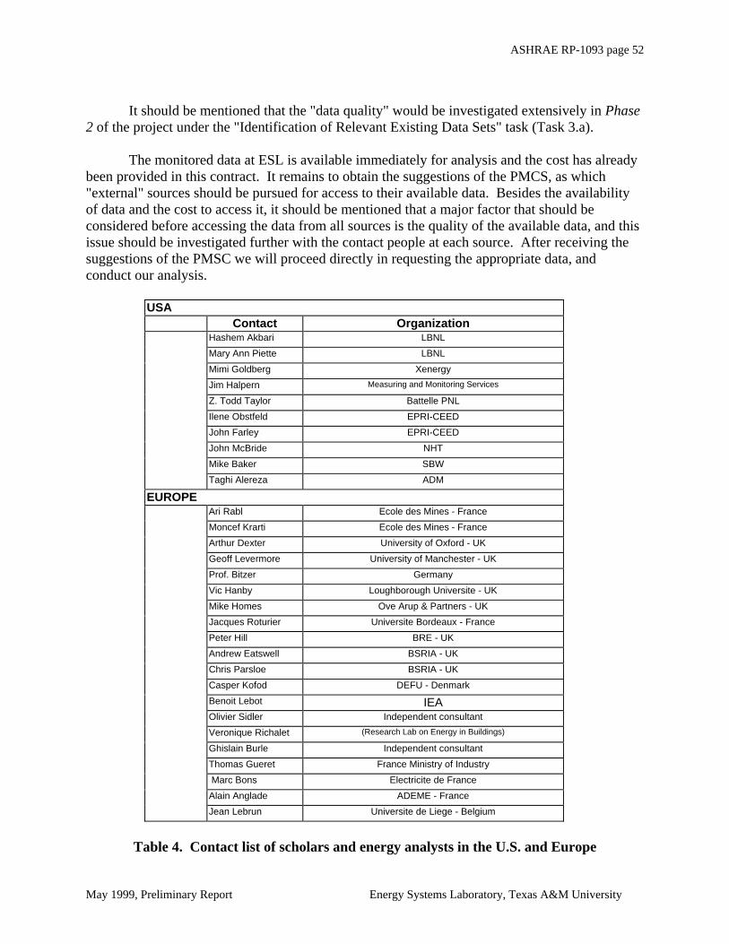
ASHRAE RP-1093 page 52
May 1999, Preliminary Report Energy Systems Laboratory, Texas A&M University
It should be mentioned that the "data quality" would be investigated extensively in Phase
2 of the project under the "Identification of Relevant Existing Data Sets" task (Task 3.a). The monitored data at ESL is available immediately for analysis and the cost has already been provided in this contract. It remains to obtain the suggestions of the PMCS, as which "external" sources should be pursued for access to their available data. Besides the availability of data and the cost to access it, it should be mentioned that a major factor that should be considered before accessing the data from all sources is the quality of the available data, and this issue should be investigated further with the contact people at each source. After receiving the suggestions of the PMSC we will proceed directly in requesting the appropriate data, and conduct our analysis.
USA Contact Organization Hashem Akbari LBNL
Mary Ann Piette LBNL
Mimi Goldberg Xenergy
Jim Halpern Measuring and Monitoring Services
Z. Todd Taylor Battelle PNL
Ilene Obstfeld EPRI-CEED
John Farley EPRI-CEED
John McBride NHT
Mike Baker SBW
Taghi Alereza ADM
EUROPE
Ari Rabl Ecole des Mines - France
Moncef Krarti Ecole des Mines - France
Arthur Dexter University of Oxford - UK
Geoff Levermore University of Manchester - UK
Prof. Bitzer Germany
Vic Hanby Loughborough Universite - UK
Mike Homes Ove Arup & Partners - UK
Jacques Roturier Universite Bordeaux - France
Peter Hill BRE - UK
Andrew Eatswell BSRIA - UK
Chris Parsloe BSRIA - UK
Casper Kofod DEFU - Denmark
Benoit Lebot IEA Olivier Sidler Independent consultant
Veronique Richalet (Research Lab on Energy in Buildings)
Ghislain Burle Independent consultant
Thomas Gueret France Ministry of Industry
Marc Bons Electricite de France
Alain Anglade ADEME - France
Jean Lebrun Universite de Liege - Belgium
Table 4. Contact list of scholars and energy analysts in the U.S. and Europe

ASHRAE RP-1093 page 53
May 1999, Preliminary Report Energy Systems Laboratory, Texas A&M University
Name Organization Data Available Remarks Cost Europe Jean Lebrun Universite de Liege - Belgium European Ministry Council Building Brussels - Belgium, Available "with or without financial support"
Guislain Burle MD3E Database of Office Equipment Use France, Available "cost depends on type of data"
Casper Kofod DEFU - Danmark Office Equipment, Lighting, Will get back to us on May 11 99 ?
Occupancy
USA Mimi Goldberg Xenergy Waiting for final answer Data belongs to clients ?
(100's of buildings)
Jim Halpern Measuring and Monitoring Services Waiting for final answer (100's ?
of buildings) Ilene Obstfeld EPRI-CEED Load shapes for several categories Southwestern Utilities (Waiting for final answer) John Farley EPRI-CEED Load shapes for Offices BC-Hydro - Canada (Waiting for final answer) Z. Todd Taylor Battelle PNL Whole building and submetered ELCAP data Probable charge channels (90 Commercial buildings)
Mary Ann Piette LBNL We are waiting to hear back Mike Baker SBW We are waiting to hear back John McBride NHT 5 to 10 commercial buildings in ? ? Montana and California
Taghi Alereza ADM More than 10 buildings in ? ? California and Louisiana
Table 5. Response obtained from the list of contacts who have data in the U.S. and Europe which will (or may) be available
for use in RP-093 (complete contact information is provided in the Appendix)

ASHRAE RP-1093 page 54
May 1999, Preliminary Report Energy Systems Laboratory, Texas A&M University
Bldg. Type Re-gion
Sam-ple
Total Load HVAC Cooling Heating Electric Water
Heating
Food Service Lighting - Exterior
Lighting - Interior
Refrigeration Other
Education NE 5 NW 4 4 1 3 3 4 4 4 4 5 SE 52 52 41 11 22 12 2 21 117 SW W Entertain NE -ment NW SE 8 8 8 4 3 2 3 15 SW W Grocery / NE Food Store NW 8 8 2 6 6 7 8 8 8 14 SE 12 12 12 5 3 4 8 10 25 SW 5 5 3 4 5 5 4 W Healthcare NE 2 2 NW SE 5 5 1 4 2 1 13 SW W 3 Hotel / Motel NE NW SE 12 11 1 1 2 5 33 SW W 3 Office NE 24 18 NW 17 17 9 14 15 15 17 17 6 28 SE 100 100 90 5 37 4 9 54 158 SW 23 23 21 21 4 4 21 6 W 9 Restaurant NE NW 6 6 6 3 2 4 6 6 6 6 7 SE 17 5 19 2 5 5 3 5 7 65 SW W Retail NE 4 28 NW 15 15 8 13 13 2 11 13 6 24 SE 88 88 79 4 22 1 13 66 5 161 SW 18 18 15 17 5 7 15 W 2
Table 6. List of available commercial building metered load data at EPRI-CEED (Data presented as obtained from EPRI-CEED. Sample sizes do not match with number of metered end-uses for some building categories; we assume
that the sample size figures should be updated to match with number of metered end-uses)

ASHRAE RP-1093 page 55
May 1999, Preliminary Report Energy Systems Laboratory, Texas A&M University
ID# Organization Building Type Sample Size (buildings) Meas'd Light/Equip Data Format Available to Charge Data Medium
1 135 Battelle Pacific Northwest All Commercial 300 - 999 Light., Equip. 5 min, 15 min, Through BPA or No Tape
Laboratory Hourly FOIA
2 213 Seattle City Light Large Offices 1 - 9 Light. ? ? ? ?
3 362 Omaha Public Power District All Commercial 300 - 999 Light., Equip. 5 min, 15 min Upon Request Nominal Disk
Fee
4 367 Energy Systems Laboratory Large Offices, Small Offices, Schools, 50 - 99 (ASHRAE FIND) Light. Equip. 15 min, Hourly General Public, Fee Disk, Tape
Colleges, Grocery Stores, Health Facilities (365 total as of April 99) ASHRAE Charged
5 650.3 The Fleming Group Large Offices, Small Offices, Warehouses, 1 - 9 Light. 15 min ? ? ?
Schools
6 650.4 The Fleming Group All Commercial 10 - 49 Light. Hourly ? ? ?
7 650.5 The Fleming Group All Commercial 10 - 49 Light. Hourly ? ? ?
8 676 Natural Resources Defense Small Offices 1 - 9 Light., Predicted Equip. 15 min General Public, Minimum ?
Council ASHRAE Charge
9 704 Oregon Department of Restaurants, Retail Stores, Grocery Stores, 100 - 299 Equip. ? General Public No Tape
Energy Lodging
10 735 ML Systems All Commercial 11 - 25 Light. ? Limited ? Summary
Database
11 740 Lawrence Berkeley Large Offices, Small Offices, Restaurants, 10 - 49 Light., Equip. Hourly General Public No (BPA Tape
Laboratory Retail Stores, Schools, Health Facil., Lodg. Approval)
12 750 Sierra Pacific Power Large Offices, Small Offices, Retail Stores, 100 - 299 Light., Equip. 15 min CEED No ?
Company Grocery Stores, Schools, Lodging
13 813 CEI Large Offices 1 - 9 Light. Hourly ? ? ?
14 760 BC Hydro & Power Large Offices, Small Offices, Restaurants, Retail St., 300 - 999 Light., Equip. 15 min ? ? ?
Authority Grocery St., Schools, Colleges, Health Facil., Lodging
15 804.1 Seattle City Light Small Offices, Retail Stores, Health Facilities 1 - 9 Light. Hourly ? ? ?
16 1055 Northwest Energy Grocery Stores 10 - 49 Light. 5 min With Owner ? ?
Permission
17 1061 University of Calgary Large Offices 1 - 9 Light. ? ? ? ?
Faculty of Environ. Design
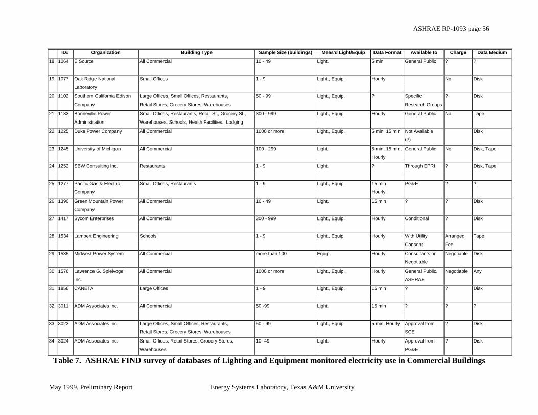
ASHRAE RP-1093 page 56
May 1999, Preliminary Report Energy Systems Laboratory, Texas A&M University
ID# Organization Building Type Sample Size (buildings) Meas'd Light/Equip Data Format Available to Charge Data Medium
18 1064 E Source All Commercial 10 - 49 Light. 5 min General Public ? ?
19 1077 Oak Ridge National Small Offices 1 - 9 Light., Equip. Hourly No Disk
Laboratory
20 1102 Southern California Edison Large Offices, Small Offices, Restaurants, 50 - 99 Light., Equip. ? Specific ? Disk
Company Retail Stores, Grocery Stores, Warehouses Research Groups
21 1183 Bonneville Power Small Offices, Restaurants, Retail St., Grocery St., 300 - 999 Light., Equip. Hourly General Public No Tape
Administration Warehouses, Schools, Health Facilities., Lodging
22 1225 Duke Power Company All Commercial 1000 or more Light., Equip. 5 min, 15 min Not Available Disk
(?)
23 1245 University of Michigan All Commercial 100 - 299 Light. 5 min, 15 min, General Public No Disk, Tape
Hourly
24 1252 SBW Consulting Inc. Restaurants 1 - 9 Light. ? Through EPRI ? Disk, Tape
25 1277 Pacific Gas & Electric Small Offices, Restaurants 1 - 9 Light., Equip. 15 min PG&E ? ?
Company Hourly
26 1390 Green Mountain Power All Commercial 10 - 49 Light. 15 min ? ? Disk
Company
27 1417 Sycom Enterprises All Commercial 300 - 999 Light., Equip. Hourly Conditional ? Disk
28 1534 Lambert Engineering Schools 1 - 9 Light., Equip. Hourly With Utility Arranged Tape
Consent Fee
29 1535 Midwest Power System All Commercial more than 100 Equip. Hourly Consultants or Negotiable Disk
Negotiable
30 1576 Lawrence G. Spielvogel All Commercial 1000 or more Light., Equip. Hourly General Public, Negotiable Any
Inc. ASHRAE
31 1856 CANETA Large Offices 1 - 9 Light., Equip. 15 min ? ? Disk
32 3011 ADM Associates Inc. All Commercial 50 -99 Light. 15 min ? ? ?
33 3023 ADM Associates Inc. Large Offices, Small Offices, Restaurants, 50 - 99 Light., Equip. 5 min, Hourly Approval from ? Disk
Retail Stores, Grocery Stores, Warehouses SCE
34 3024 ADM Associates Inc. Small Offices, Retail Stores, Grocery Stores, 10 -49 Light. Hourly Approval from ? Disk
Warehouses PG&E
Table 7. ASHRAE FIND survey of databases of Lighting and Equipment monitored electricity use in Commercial Buildings

ASHRAE RP-1093 page 57
May 1999, Preliminary Report Energy Systems Laboratory, Texas A&M University
2.4 CLASSIFICATION OF COMMERCIAL BUILDINGS Commercial buildings are classified according to different criteria by national standards and agencies. In the following we list the major classification schemes that are currently followed in the industry. 2.4.a Summary In the following we list major classification schemes of the commercial building sector that were used by various national laboratories and agencies, and published in standards. Our survey of the classification schemes covered: ASHRAE FIND (ASHRAE 1995), ASHRAE Standard 90.1(ASHRAE 1989), CBECS (CBECS 1997a and b), NAICS (NAICS 1997), ELCAP (ELCAP 1989 and Gillman et al. 1990), BECA (Wall et al. 1984), and EPRI -CEED (personal communication with Mr. John Farley). 2.4.a.1 ASHRAE FIND ASHRAE FIND (1995) database of measured energy use in the U.S. and Canada provided a source of commercial buildings classification, in the way the results of the conducted survey were categorized under the "Commercial Buildings" category. The classification scheme appeared as follows:
• Large Offices • Small Offices • Restaurants • Retail Stores • Grocery Stores • Warehouses • Schools • Colleges • Health Facilities • Lodging. The database does not explain how the "Large Offices" and "Small office" are defined in terms of floors of square footage.
2.4.a.2 ASHRAE Standard 90.1
ASHRAE Standard 90.1 (ASHRAE 1989) divided the Commercial Buildings stock in the following categories:
• Assembly • Food Service • Fast Food / Cafeteria • Leisure Dining / Bar • Offices • Retail • Schools

ASHRAE RP-1093 page 58
May 1999, Preliminary Report Energy Systems Laboratory, Texas A&M University
• Preschool / Elementary • Jr. High / High School • Technical / Vocational • Hotel / Motel • Health Care / Institutional • Warehouse Office buildings are divided in separate categories based on the gross area. However, the
square footage defining the categories changes as the purpose of categorizing the buildings change. For instance, for establishing the Prescriptive Unit Lighting Power Allowance (ULPA), W/ft2, the Offices are divided into six categories following this scheme: 0 to 2,000 ft2 2,001 to 10,000 ft2 10,001 to 25,000 ft2 25,001 to 50,000 ft2 50,001 to 250,000 ft2 > 250,000 ft2
For establishing the Average Receptacle Power Densities, W/ft2, the Offices are not considered in subcategories as in the lighting densities scheme. There is one "Office" category only. For establishing the Occupancy densities, ft2/person, there is also one "Office" category only. In establishing the HVAC systems and energy types for prototype buildings, the Offices are divided as follows: 0 ft2 to 20,000 ft2 20,001 ft2 and < 3 floors, or 20,001 to 75,000 ft2 > 75,000 ft2 or > 3 floors
However, for the Occupancy and Lighting and Receptacles Diversity Factors, Offices are
considered as one category only. 2.4.a.3 CBECS This section summarizes basic statistics of the commercial buildings stock in the USA, as published in the CBECS - Commercial Buildings Characteristics 1995 (CBECS 1997-a), and Commercial Buildings Energy Consumption and Expenditures 1995 (CBECS 1997-b), which are relevant to the current project. We included this section in the report to emphasize the criteria behind defining different subcategories of the commercial building stock. Each subcategory is meaningful in terms of the characteristics of operation, size of sample, square footage, energy use, diversity of end-use, and climate zone. These statistics on the commercial building stock in
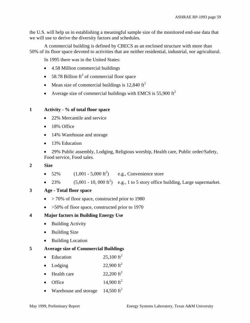
ASHRAE RP-1093 page 59
May 1999, Preliminary Report Energy Systems Laboratory, Texas A&M University
the U.S. will help us in establishing a meaningful sample size of the monitored end-use data that we will use to derive the diversity factors and schedules.
A commercial building is defined by CBECS as an enclosed structure with more than 50% of its floor space devoted to activities that are neither residential, industrial, nor agricultural.
In 1995 there was in the United States:
• 4.58 Million commercial buildings
• 58.78 Billion ft2 of commercial floor space
• Mean size of commercial buildings is 12,840 ft2
• Average size of commercial buildings with EMCS is 55,900 ft2
1 Activity - % of total floor space
• 22% Mercantile and service
• 18% Office
• 14% Warehouse and storage
• 13% Education
• 29% Public assembly, Lodging, Religious worship, Health care, Public order/Safety, Food service, Food sales.
2 Size
• 52% (1,001 - 5,000 ft2) e.g., Convenience store
• 23% (5,001 - 10, 000 ft2) e.g., 1 to 5 story office building, Large supermarket.
3 Age - Total floor space
• > 70% of floor space, constructed prior to 1980
• >50% of floor space, constructed prior to 1970
4 Major factors in Building Energy Use
• Building Activity
• Building Size
• Building Location
5 Average size of Commercial Buildings
• Education 25,100 ft2
• Lodging 22,900 ft2
• Health care 22,200 ft2
• Office 14,900 ft2
• Warehouse and storage 14,500 ft2
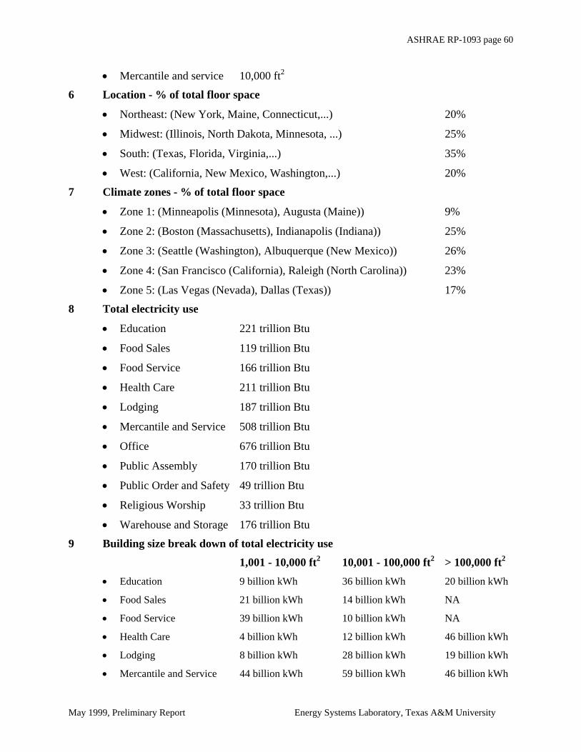
ASHRAE RP-1093 page 60
May 1999, Preliminary Report Energy Systems Laboratory, Texas A&M University
• Mercantile and service 10,000 ft2
6 Location - % of total floor space
• Northeast: (New York, Maine, Connecticut,...) 20%
• Midwest: (Illinois, North Dakota, Minnesota, ...) 25%
• South: (Texas, Florida, Virginia,...) 35%
• West: (California, New Mexico, Washington,...) 20%
7 Climate zones - % of total floor space
• Zone 1: (Minneapolis (Minnesota), Augusta (Maine)) 9%
• Zone 2: (Boston (Massachusetts), Indianapolis (Indiana)) 25%
• Zone 3: (Seattle (Washington), Albuquerque (New Mexico)) 26%
• Zone 4: (San Francisco (California), Raleigh (North Carolina)) 23%
• Zone 5: (Las Vegas (Nevada), Dallas (Texas)) 17%
8 Total electricity use
• Education 221 trillion Btu
• Food Sales 119 trillion Btu
• Food Service 166 trillion Btu
• Health Care 211 trillion Btu
• Lodging 187 trillion Btu
• Mercantile and Service 508 trillion Btu
• Office 676 trillion Btu
• Public Assembly 170 trillion Btu
• Public Order and Safety 49 trillion Btu
• Religious Worship 33 trillion Btu
• Warehouse and Storage 176 trillion Btu
9 Building size break down of total electricity use
1,001 - 10,000 ft2 10,001 - 100,000 ft2 > 100,000 ft2 • Education 9 billion kWh 36 billion kWh 20 billion kWh
• Food Sales 21 billion kWh 14 billion kWh NA
• Food Service 39 billion kWh 10 billion kWh NA
• Health Care 4 billion kWh 12 billion kWh 46 billion kWh
• Lodging 8 billion kWh 28 billion kWh 19 billion kWh
• Mercantile and Service 44 billion kWh 59 billion kWh 46 billion kWh

ASHRAE RP-1093 page 61
May 1999, Preliminary Report Energy Systems Laboratory, Texas A&M University
• Office 30 billion kWh 76 billion kWh 92 billion kWh
• Public Assembly 7 billion kWh 27 billion kWh 16 billion kWh
• Public Order and Safety 1 billion kWh 9 billion kWh NA
• Religious Worship 4 billion kWh 6 billion kWh NA
• Warehouse and Storage 11 billion kWh 22 billion kWh 19 billion kWh
10 Lighting Equipment - % of total lit floor space
• Standard Fluorescent 96%
• Incandescent 63%
• High Intensity Discharge 30%
• Compact Fluorescent 26%
• Halogen 18%
11 Lighting Equipment vs. Average size of buildings
• High Intensity Discharge 41,000 ft2
• Compact Fluorescent 39,200 ft2
• Halogen 32,000 ft2
(Average size of commercial buildings: 12,840 ft2)
12 Peak Watt/ft2 - Activity
• Education 4.29 W/ft2
• Food Sales 14.67 W/ft2
• Food Service 12.67 W/ft2
• Health Care 5.89 W/ft2
• Lodging 4.89 W/ft2
• Mercantile and Service 4.91 W/ft2
• Office 6.00 W/ft2
• Public Assembly 5.52 W/ft2
• Public Order and Safety 5.00 W/ft2
• Religious Worship 4.20 W/ft2
• Warehouse and Storage 2.22 W/ft2
13 Peak Watt/ft2 - Climate zone
• < 2,000 CDD and > 7,000 HDD 5.78 W/ft2
• 5,500 - 7,000 HDD 5.00 W/ft2

ASHRAE RP-1093 page 62
May 1999, Preliminary Report Energy Systems Laboratory, Texas A&M University
• 4,000 - 5,499 HDD 4.00 W/ft2
• < 4,000 HDD 6.67 W/ft2
• > 2,000 CDD and < 4,000 HDD 5.41 W/ft2
2.3.a.4 NAICS (new SIC) The North American Industry Classification System (NAICS 1997) is the government classification system that replaces the Standard Industrial Classification (SIC) that was used in the United States for the last 60 years. The new classification system is more global than the precious one in order to cover the industries in Canada and Mexico as well. The NAICS defines all sectors of Industries, and touches the Construction sector. Under Construction (Sector 23), the "Building, Developing, and General Contracting" (Subsector 233) comprises the Category 233320 "Commercial and Institutional Building Construction" which is defines as follows:
"…. This industry comprises establishments primarily responsible for the entire construction (i.e., new work, additions, alterations, and repairs) of commercial and institutional buildings (e.g., stores, schools, hospitals, office buildings, public warehouses. …." The following categories are listed under Commercial and Institutional Building
Construction (we are not showing the term "construction" in each category, for briefness): • Administration building • Amusement building • Bank building • Casino building • Church, synagogue, mosque, temple, and related building • Cinema • Farm building • Hospital • Hotel • Municipal building • Office building • Prison • Public warehouse • Restaurant • School building • Service station • Shopping center or mall
2.4.a.5 ELCAP ELCAP (End-use Load and Consumer Assessment Program) database of commercial buildings loads contains hourly whole-building electricity consumption and several sub-metered channels for 90 buildings approximately. The data was grouped according to the building type and is associated with the location (city, state), square footage, and address information. Further contact with ELCAP, through personal communication with Mr. Z. Todd Taylor is planned to

ASHRAE RP-1093 page 63
May 1999, Preliminary Report Energy Systems Laboratory, Texas A&M University
specify the building types ELCAP used, and also to decide on the cost that will incur in obtaining their data. We have reviewed the paper written by Pratt et al. (1990), in which they report the work done in the ELCAP commercial building metering project. They categorized and monitored 17 different en-uses, and they divided the commercial buildings category in 11 subcategories. 2.4.a.6 BECA The Building Energy-Use Compilation and Analysis (BECA) is a project conducted by Lawrence Berkeley Laboratory. It included compilations on the energy performance and cost-effectiveness of low-energy homes (BECA-A), existing "retrofitted" homes (BECA-B), energy-efficient new commercial buildings (BECA-CN), existing "retrofitted" commercial buildings (BECA-CR), appliances and equipment (BECA-D), and validations of building performance models (BECA-V). Under BECA-CN 83 buildings were measured, and the majority were large or small office buildings, or schools. The stated that these building categories presented in the study represented 19% of the U.S. commercial building stock, and conversely, other major building types were not represented in BECA-CN. The major building categories that were not represented and was worth studying were:
• Retail • Grocery/Restaurant • Assembly • Warehouse
2.4.a.7 EPRI EPRI's Center for Energy End-use Data (CEED) provides products and services including monitored end-uses in commercial buildings, and derived typical load shapes. The CEED commercial building metered load data is categorized according to U.S. geographic locations, end-use type, and building groups. The geographic locations are: (1)Northeast, (2)Northwest, (3)Southeast, (4)Southwest, and (5) West. The end-use types are: (1) Total load, (2) HVAC, (3) Cooling, (4) Heating, (5) Electric Water Heating, (6) Food Service, (7) Lighting-Exterior, (8) Lighting-Interior, (9) Refrigeration, and (10) Other. The commercial building groups are:
• Education • Entertainment • Grocery / Food Store • Healthcare • Hotel / Motel • Office • Restaurant • Retail
2.4.b Recommendations We are proposing to follow the classification followed by the Commercial Buildings Energy Consumption Survey (CBECS), a national survey of commercial buildings and their energy suppliers, in compiling their statistics of the commercial building stock in the U.S. We

ASHRAE RP-1093 page 64
May 1999, Preliminary Report Energy Systems Laboratory, Texas A&M University
based our proposal on the detailed compiled survey results of CBECS, that helped us in drawing meaningful conclusions. The CBECS classification scheme agrees with that of ASHRAE Standard 90.1, taking into consideration the small representation, in the whole commercial building stock, of the "Religious Worship" and the "Public Order and Safety" categories that appear in the CBECS classification. Therefore the commercial building classification that we will follow in developing the diversity factors and schedules for energy and cooling load calculations will consist of the following categories:
0. Offices 1. Education 2. Health Care 3. Lodging 4. Food Service 5. Food Sales 6. Mercantile and Services 7. Public Assembly 8. Warehouse and Storage
We will start our analysis with Office buildings (according to the RFP), and divide the
Office buildings subcategory in three different groups: • Small (1,001 - 10,000 ft2) • Medium (10,001 - 100,000 ft2) • Large (> 100,000 ft2). After consultation with the PMSC, we will determine if additional categories in the
commercial building sector should be included in the study. 2.4.c Fitting Existing Databases into Commercial Buildings Categories We have located many sources of monitored commercial buildings lighting and equipment monitored data in the U.S. and some in Europe. Upon determining out the quality of the data available and its relevance to our ASHRAE 1093-RP work, and its cost, we are planning to fit the appropriate data into the defined commercial buildings categories, for the best representation of available data that meets ASHRAE PMSC needs. 0. PROPOSED METHODOLOGY
In the next phases of this project we will carry out the following tasks:
0.0 Relevant Data Sets From the available data sets that we located in the U.S. and Europe, we will determine

ASHRAE RP-1093 page 65
May 1999, Preliminary Report Energy Systems Laboratory, Texas A&M University
the quality and the relevance of those sets that will be tested for this project and used for producing the final compiled library of diversity factors and schedules. In choosing the data sets, we will also take into consideration the geographic location in order to obtain a meaningful sample representing various climatic zones of the united states, which might be reflected indirectly in the pattern of the lighting and equipment load shapes.
1.0 Classification Methods
After the consultation with the PMSC, we will include a standard building classification section in the final project report, which will illustrate and simplify the use of the diversity factors and the load shapes. We already reviewed the classification schemes of the commercial building categories and subcategories, and provided our recommendations in this concern (Section 2.4.b above).
2.0 Relevant Statistical Procedures for Daytyping
We have identified different methods used for daytyping and determination of load shapes used in the U.S. and Europe for weather dependent and weather independent energy uses. We categorized these methods in groups of approaches. We will test these methods with the data provided in ASHRAE Shootout I and II, and determine their relevance to the project. After consultation with the PMSC, we will adopt the chosen methodologies to the relevant data set and derive the diversity factors and load shapes.
3.0 Robust Uncertainty Analysis Methodology
The ESL has been investigating issues of uncertainty relating to field data (Reddy et al. 1992; Reddy et a. 1997). We will conduct a survey of other methods reported in the literature and perform a preliminary uncertainty analysis after identifying the relevant energy use data sets and statistical procedures for daytyping, to help determine the required quality of the general use of the derived diversity factors. An uncertainty analysis will also accompany the final project results.
4.0 Compilation of Diversity Factors and Load Shapes We will evaluate and refine our approach(es) in deriving the diversity factors and load shapes by assessing the reliability and the uncertainty of the methods used. A library of the derived diversity factors and load shapes will be derived for energy and cooling load calculations in various types of indoor environments. The library will include a robust uncertainty analysis on the statistically derived results.
ASHRAE RP-1093 page 66
May 1999, Preliminary Report Energy Systems Laboratory, Texas A&M University
5.0 Development of a Tool-Kit and General Guidelines for Deriving New Diversity Factors
We will prepare a Tool-Kit of computer codes in both fully commented source and executable versions, which are necessary for deriving new diversity factors. After receiving the approval of the PMS on the codes, as of the technical content and the compliance with ASHRAE TC 1.5 requirements, we will prepare final versions to be included in the final report. We will also submit General Guidelines on the application of the diversity factors and load shapes to various types of buildings and office environments. 6.0 Development of Examples of the Use of Diversity Factors in DOE-2 and BLAST
Simulation Programs As requested in the RFP, we shall provide illustrative examples of how such diversity factors are to be input into the DOE-2 and BLAST programs. 4. CONCLUDING REMARKS We have completed our literature survey of the available metered end-uses in the commercial building sector in the U.S. and Europe. We have also completed the survey of the methods used in daytyping and determining the load shape factors of commercial (and few residential, for their potential applicability to the commercial buildings), in the U.S. and Europe. Three papers from Europe explained the methods utilized in developing the load shapes. We will identify the relevant methods to determining the lighting/equipment/occupancy diversity factors and test them against the AHRAE Shootout I and II data sets. We also reviewed all schemes of commercial building classification as reported in published projects, and listed in national codes and standards. Phase 2 of the project will be based on our findings reported in this preliminary report, and will be carried out in accordance with the PMSC's comments on this report. 5. REFERENCES 822-RP. Test method for measuring the heat gain and radiant/convective split from equipment in buildings. American Society of Heating, Refrigeration and Air-Conditioning Engineers, Atlanta, Georgia. Akbari, H., J. Eto, S. Konopacki, K. Heinemeier, and L. Rainer. 1994. A new approach to estimate commercial sector end-use load shapes and energy use intensities. Proceedings of the 1994 ACEEE Summer Study on Energy Efficiency in Buildings, pp. 2.2-2.10.

ASHRAE RP-1093 page 67
May 1999, Preliminary Report Energy Systems Laboratory, Texas A&M University
Akbari, H., Heinemeier, K., Le Coniac, P., and Flora, D. 1988. An algorithm to disaggregate commercial whole-building electric hourly load into end-uses. Proceedings of the 1988 ACEEE Summer Study on Energy Efficiency in Buildings, pp. 10.13-10.36. Akbari, H., Turiel, I., Eto, J., Heinemeier, K., and Lebot, B. 1990. A review of existing commercial energy use intensity and load shapes studies. Proceedings of the 1990 ACEEE Summer Study on Energy Efficiency in Buildings, pp. 3.7-3.18. Alereza, T., and Faramarzi, R., 1994. More data is better, but how much is enough for impact evaluations? Proceedings of the 1994 ACEEE Summer Study on Energy Efficiency in Buildings, pp. 2.11-2.19. ASHRAE 1989. ASHRAE Standard 90.1. Energy Efficient Design of New Buildings Except Low-Rise Residential Buildings. American Society of Heating, Refrigeration and Air-Conditioning Engineers, Atlanta, Georgia. ASHRAE 1991. ASHRAE Handbook of HVAC Applications. American Society of Heating, Refrigeration and Air-Conditioning Engineers, Atlanta, Georgia. ASHRAE 1995. ASHRAE FIND, An inventory of Measured Energy-use databases (a diskette and a user manual). American Society of Heating, Refrigeration and Air-Conditioning Engineers, Atlanta, Georgia. Baker, M. 1990. Utility application of commercial sector end-use load measurements: Case studies are not good enough!. Proceedings of the 1990 ACEEE Summer Study on Energy Efficiency in Buildings, pp. 3.27-3.34. Baker, M. and Guliasi, L. 1988. Alternative approaches to end-use metering in the commercial sector: The design of Pacific Gas and Electric Company's commercial end-use metering project. Proceedings of the 1988 ACEEE Summer Study on Energy Efficiency in Buildings, pp. 10.28-10.41. Barrar, J., Ellison, D., Wikler, G., and Hamzawi, E. 1992. Integrating engineering-based modeling into commercial-sector DSM program planning. Proceedings of the 1992 ACEEE Summer Study on Energy Efficiency in Buildings, pp. 3.23-3.32. Bou-Saada, T.E., Haberl, J.S., Vajda, E.J., Shincovich, M., D'Angelo, L., and Harris, L. 1996. Total utility savings from the 37,000 fixture lighting retrofit to the U.S. DOE Forrestal Building. Proceedings of the 1996 ACEEE Summer Study on Energy Efficiency in Buildings, pp. 4.31-4.48. Bou-Saada, T.E., and J.S. Haberl. 1995. A weather-daytyping procedure for disaggregating hourly end-use loads in an electrically heated and cooled building from whole-building hourly data. Proceedings of the 30th Intersociety Energy Conversion Engineering Conference, July 31-August 4 1995, Orlando, FL, pp. 323-330.

ASHRAE RP-1093 page 68
May 1999, Preliminary Report Energy Systems Laboratory, Texas A&M University
Bronson, D.J., S. Hinshey, J.S. Haberl, and D.L. O’Neal. 1992. A procedure for calibrating the DOE-2 simulation program to non-weather-dependent measured loads. ASHRAE Transactions 98 (1). CBECS 1997-a. Commercial buildings characteristics 1995. Commercial Buildings Energy Consumption Survey (CBECS), Energy Information Administration (EIA), Office of Energy Markets and End Use, USDOE, August 1997. CBECS 1997-b. Commercial Buildings Energy Consumption and Expenditures 1995. Commercial Buildings Energy Consumption Survey (CBECS), Energy Information Administration (EIA), Office of Energy Markets and End Use, USDOE, 1995. CEED 1995. Leveraging limited data resources: Developing commercial end-use information: BC Hydro case study. Technical Report. EPRI's Center for Electric End-Use Data (CEED). Portland, Oregon. De Almeida, A.T., Saraiva, N., Roturier, J., Anglade, A., and Jensen, M. 1998. Management of the electricity consumption in the office equipment end-use for an improved knowledge of usage in the tertiary sector in Europe. Proceedings of the 1998 ACEEE Summer Study on Energy Efficiency in Buildings, pp. 5.35-5.47. De La Hunt, M.J. 1990. Trends in electricity consumption due to computers and miscellaneous equipment (CME) in office buildings. Proceedings of the 1990 ACEEE Summer Study on Energy Efficiency in Buildings, pp. 3.67-3.75. EIA-DOE. 1992. Lighting in commercial buildings. Energy Consumption Series. Energy Information Administration, Office of Energy Markets and End Use, USDOE., March 1992. ELCAP. 1989. Description of electric energy use in single-family residences in the Pacific Northwest. End-use Load and Consumer Assessment Program (ELCAP). Pacific Northwest Laboratory, Richland, Washington. EPRI 1999. EPRI's Southeast Data Exchange. Information obtained from EPRI-CEED website. Center for Electric End-Use Data (CEED). Portland, Oregon. Emery, A.F., and Gartland, L.M. 1996. Quantifying occupant energy behavior using pattern analysis techniques. Proceedings of the 1996 ACEEE Summer Study on Energy Efficiency in Buildings, pp. 8.47-8.59. Eto, J.H., Akbari, H., Pratt, R., and Braithwait, S. 1990. End-use load shape data: Application, estimation, and collection. Proceedings of the 1990 ACEEE Summer Study on Energy Efficiency in Buildings, pp. 10.39-10.55. Finleon, J. 1990. A method for developing end-use load shapes without end-use metering. Proceedings of the 1990 ACEEE Summer Study on Energy Efficiency in Buildings, pp. 10.57-10.65.

ASHRAE RP-1093 page 69
May 1999, Preliminary Report Energy Systems Laboratory, Texas A&M University
Floyd, D.B., Parker, D.S., and Sherwin, J.R. 1996. Measured field performance and energy savings of occupancy sensors: Three case studies. Proceedings of the 1996 ACEEE Summer Study on Energy Efficiency in Buildings, pp. 4.97-4.105. Gillman, R., Sands, R.D., and Robert, G.L. 1990. Observations on residential and commercial load shapes during a cold snap. Proceedings of the 1990 ACEEE Summer Study on Energy Efficiency in Buildings, pp. 10.81-10.89. Haberl, J.S., and Claridge, D.E. 1987. An expert system for building energy consumption analysis: Prototype results. ASHRAE Transactions 1987, V.93, Pt.1, pp. 979-998. Haberl, J.S., and P. Komor. 1989. Investigating an analytical basis for improving commercial building energy audits: Results from a New Jersey mall. Center for Energy and Environmental Studies Report No. 264, June 1989. Haberl, J.S., and Komor, P.S. 1990a. Improving commercial building energy audits: How annual and monthly consumption data can help. ASHRAE Journal. August 1990, pp.26-33. Haberl, J.S., and Komor, P.S. 1990b. Improving commercial building energy audits: How daily and hourly consumption data can help. ASHRAE Journal. September 1990, pp.26-36. Haberl, J.S., and Thamilseran, S, 1996. The Great Energy Predictor Shootout II: Measuring retrofit savings - Overview and discussion. ASHRAE Transaction 1996, V. 102, Pt. 2. Hadley, D.L. 1993. Daily variations in HVAC system electrical energy consumption in response to different weather conditions. Energy and Buildings, V.19 (1993), pp. 235-247. Halverson, M.A., Stoops, J.L., Schmelzer, J.R., Chvala, W.D., Keller, J.M., and Harris, L.R. 1994. Lighting retrofit monitoring for the federal sector - Strategies and results at the DOE Forrestal Building. Proceedings of the 1994 ACEEE Summer Study on Energy Efficiency in Buildings, pp. 2.137-2.144. Hamzawi, E. H., and Messenger, M., 1994. Energy and peak demand impact estimates for DSM technologies in the residential and commercial sectors for California: Technical and regulatory perspectives. Proceedings of the 1994 ACEEE Summer Study on Energy Efficiency in Buildings, pp. 2.145-2.155. Heidell, J.A. 1984. Development of a data base on end-use energy consumption in commercial buildings. Proceedings of the 1984 ACEEE Summer Study on Energy Efficiency in Buildings, pp. D-49 - D-62. Jacobs, P.C., Waterbury, S.S., Frey, D.J., and Johnson, K.F. 1994. Short-term measurements to support impact evaluation of commercial lighting programs. Proceedings of the 1994 ACEEE Summer Study on Energy Efficiency in Buildings, pp. 5.113-5.121.

ASHRAE RP-1093 page 70
May 1999, Preliminary Report Energy Systems Laboratory, Texas A&M University
Katipamula, S., Allen, T., Hernandez, G., Piette, M.A., and Pratt, R.G. 1996. Energy savings from Energy Star personal computer systems. Proceedings of the 1996 ACEEE Summer Study on Energy Efficiency in Buildings, pp. 4.211-4.218. Katipamula, S., and J.S. Haberl. 1991. A methodology to identify diurnal load shapes for non-weather dependent electric end-uses. Proceedings of the 1991 ASME-JSES International Solar Energy Conference, New York, N.Y., pp. 457-467. Keith, D.M., and Krarti, M. 1999. Simplified prediction tool for peak occupancy rate in office buildings. Journal of the Illuminating Engineering Society, Winter 1999, pp. 43-52. Komor, P. 1997. Space cooling demands from office plug loads. ASHRAE Journal (December). Kreider, J.F., and Haberl, J.S. 1994. Predicting hourly building energy use: The Great Energy Predictor Shootout - Overview and discussion of results. ASHRAE Transactions 1994, V.100, Pt. 2. Margossian, B. 1994. Deriving end-use load profiles without end-use metering: Results of recent validation studies. Proceedings of the 1994 ACEEE Summer Study on Energy Efficiency in Buildings, pp. 2.218-2.223. Mazzucchi, R.P. 1992. End-use profile development from whole-building data combined with intensive short-term monitoring. ASHRAE Transactions 1992, V.98, Pt.1, pp. 1180-1184. NAICS 1997. North American Industry Classification System. Office of Management and Budget, Executive Office of the President, United States Government, JIST edition. Nordman, B., M.A. Piette, and K. Kinney. 1996. Measured energy savings and performance of power-managed personal computers and monitors. Proceedings of the 1996 ACEEE Summer Study on Energy Efficiency in Buildings, pp. 4.267-4.278. Noren, C., and Pyrko, J. 1998. Typical load shapes for Swedish schools and hotels. Energy and Buildings. Volume 28, Number 3, 1998, pp.145-157. Norford, L.K., Rabl, A., Harris, J., and Roturier, J. 1988. The sum of Megabytes equals Gigawatts: Energy consumption and efficiency of office PCs and related equipment. Proceedings of the 1988 ACEEE Summer Study on Energy Efficiency in Buildings, pp. 3.181-3.196. Norford, L.K., R.H. Socolow, E.S. Hsieh, and G.V. Spadaro. 1994. Two to one discrepancy between measured and predicted performance of a “low-energy” office building: insights from a reconciliation based on the DOE-2 model. Energy and Buildings, V.21 (1994), pp. 121-131. Olofsson, T., Anderson, S., and Ostin, R. 1998. Using CO2 concentrations to predict energy consumption in homes. Proceedings of the 1998 ACEEE Summer Study on Energy Efficiency in Buildings, pp. 1.211-1.222.

ASHRAE RP-1093 page 71
May 1999, Preliminary Report Energy Systems Laboratory, Texas A&M University
Owashi, L., Schiffman, D.A., and Sickels, A.D. 1994. Lighting hours of operation: Building type versus space use characteristics for the commercial sector. Proceedings of the 1994 ACEEE Summer Study on Energy Efficiency in Buildings, pp. 8.157-8.162. Parker, J.L. 1996. Developing load shapes: Leveraging existing load research data, visualization techniques, and DOE-2E modeling. Proceedings of the 1996 ACEEE Summer Study on Energy Efficiency in Buildings, pp. 3.105-3.113. Parti, M., Sebald, A.V., Charkow, J., and Flood, J. 1988. A comparison of conditional demand estimates of residential end-use load shapes with load shapes derived from end-use meters. Proceedings of the 1988 ACEEE Summer Study on Energy Efficiency in Buildings, pp. 10.203-10.218. Powers, J.T., and Martinez, M. 1992. End-use profiles from whole-house data: A rule-based approach. Proceedings of the 1992 ACEEE Summer Study on Energy Efficiency in Buildings, pp. 4.193-4.199. Pratt, R.G., Williamson, M.A., and Richman, E.E. 1990. Miscellaneous equipment in commercial buildings: The inventory, utilization, and consumption by equipment type. Proceedings of the 1990 ACEEE Summer Study on Energy Efficiency in Buildings, pp. 3.173-3.184. Rohmund, I., McMenamin, S., and Bogenrieder, P. 1992. Commercial load shape disaggregation studies. Proceedings of the 1992 ACEEE Summer Study on Energy Efficiency in Buildings, pp. 3.251-3.262. Schon, A., and Rodgers, R. 1990. An affordable approach to end-use load shapes for commercial facilities. Proceedings of the 1994 ACEEE Summer Study on Energy Efficiency in Buildings. Stoops, J., and Pratt, R. 1990. Empirical data for uncertainty reduction. Proceedings of the 1990 ACEEE Summer Study on Energy Efficiency in Buildings, pp. 6.177-6.189. Szydlowski, R.F., and W.D. Chvala. 1994. Energy consumption of personal computers. Proceedings of the 1994 ACEEE Summer Study on Energy Efficiency in Buildings, pp. 2.257-2.267. Thamilseran, S., and J.S. Haberl. 1994. A bin method for calculating energy conservation retrofit savings in commercial buildings. Proceedings of the Ninth Symposium on Improving Building Systems in Hot and Humid Climates, Dallas, TX, pp. 142-152. Thamilseran, S. 1999. An inverse bin methodology to measure the savings from energy conservation retrofits in commercial buildings. A Ph.D. dissertation in Mechanical Engineering, Texas A&M University, College Station, Texas.
ASHRAE RP-1093 page 72
May 1999, Preliminary Report Energy Systems Laboratory, Texas A&M University
Wall, L.W., Piette, M.A., and Harris, J.P. 1984. A summary report of BECA-CN: Buildings Energy use Compilation and Analysis of energy-efficient new commercial buildings. Proceedings of the 1984 ACEEE Summer Study on Energy Efficiency in Buildings, pp. D-259 - D-278. Wilkins, C.K., and N. McGaffin. 1994. Measuring computer equipment loads in office buildings. ASHRAE Journal (August). 6. BIBLIOGRAPHY Akbari, H., Eto, J., Turiel, I., Heinemeier, K., Lebot, B., Nordman, B., and Rainer, L. 1989. Integrated estimation of commercial sector end-use load shapes and energy use intensities. Final Report. Applied Science Division, Lawrence Berkeley Laboratory, University of California, Berkeley, California. Amalfi, J., Jacobs, P.C., and Wright, R.L. 1996. Short-term monitoring of commercial lighting systems - Extrapolation from the measurement period to annual consumption. Proceedings of the 1996 ACEEE Summer Study on Energy Efficiency in Buildings, pp. 6.1-6.7. ASHRAE 1993. ASHRAE Handbook of Fundamentals. American Society of Heating, Refrigeration and Air-Conditioning Engineers, Atlanta, Georgia. Diamond, R., Piette, M.A., Nordman, B., De Buen, O., and Harris, J. 1992. The performance of Energy Edge Buildings: Energy use and savings. Proceedings of the 1992 ACEEE Summer Study on Energy Efficiency in Buildings, pp. 3.47-3.60. Noren, C., and Pyrko, J. 1998. Using multiple Regression analysis to develop electricity consumption indicators for public schools. Proceedings of the 1998 ACEEE Summer Study on Energy Efficiency in Buildings, pp. 3.255-3.266. Noren, C. 1997. Typical load shapes for six categories of Swedish commercial buildings. Technical Report, Lund Institute of Technology, Department of Heat and Power Engineering, Division of Energy Economics and Planning, Lund, Sweden. Powers, J.T., and Martinez, M. 1992. End-use profiles from whole-house data: A rule-based approach. Proceedings of the 1992 ACEEE Summer Study on Energy Efficiency in Buildings, pp. 4.193-4.199. Reddy, T.A., K. Kissock, and D.E. Claridge. 1992. Uncertainty analysis in estimating building energy retrofit savings in the LoanSTAR Program. Proceedings of the 1992 ACEEE Summer Study on Energy Efficiency in Buildings, Vol.3, pp. 225-238.

ASHRAE RP-1093 page 73
May 1999, Preliminary Report Energy Systems Laboratory, Texas A&M University
Reddy, T.A., K. Kissock, and D.K. Ruch. 1997. Uncertainty in baseline regression modeling and in determination of retrofit savings. Accepted by the ASME Journal of Solar Energy Engineering. Schrock, D.W. 1997. Load shape development. Pennwell Books. Pennwell Publishing Company. Tulsa, Oklahoma, 1997. 7. APPENDIX
This appendix includes: (1) a table (Table 8) of all sites monitored, and maintained in the database of the Energy Systems Laboratory, and (2) a complete list of contacts who provided us with positive responses in terms of willingness to offer us access to their databases.
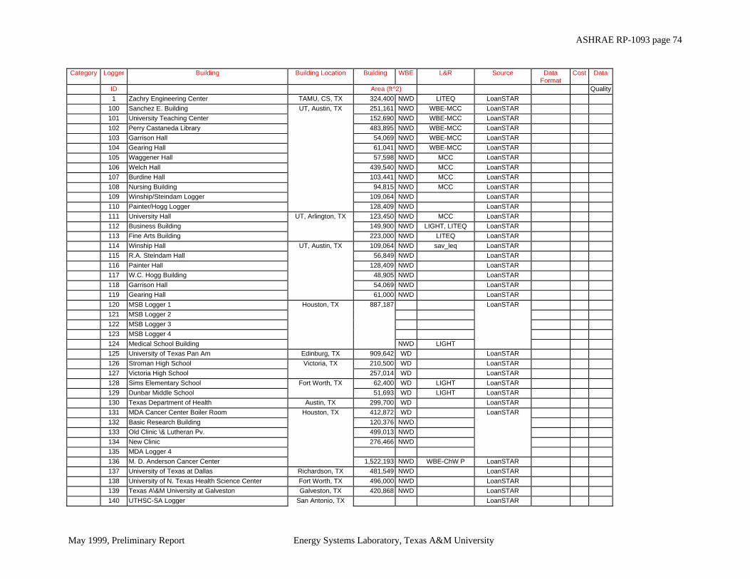
ASHRAE RP-1093 page 74
May 1999, Preliminary Report Energy Systems Laboratory, Texas A&M University
Category Logger Building Building Location Building WBE L&R Source Data Format
Cost Data
ID Area (ft^2) Quality 1 Zachry Engineering Center TAMU, CS, TX 324,400 NWD LITEQ LoanSTAR 100 Sanchez E. Building UT, Austin, TX 251,161 NWD WBE-MCC LoanSTAR 101 University Teaching Center 152,690 NWD WBE-MCC LoanSTAR 102 Perry Castaneda Library 483,895 NWD WBE-MCC LoanSTAR 103 Garrison Hall 54,069 NWD WBE-MCC LoanSTAR 104 Gearing Hall 61,041 NWD WBE-MCC LoanSTAR 105 Waggener Hall 57,598 NWD MCC LoanSTAR 106 Welch Hall 439,540 NWD MCC LoanSTAR 107 Burdine Hall 103,441 NWD MCC LoanSTAR 108 Nursing Building 94,815 NWD MCC LoanSTAR 109 Winship/Steindam Logger 109,064 NWD LoanSTAR 110 Painter/Hogg Logger 128,409 NWD LoanSTAR 111 University Hall UT, Arlington, TX 123,450 NWD MCC LoanSTAR 112 Business Building 149,900 NWD LIGHT, LITEQ LoanSTAR 113 Fine Arts Building 223,000 NWD LITEQ LoanSTAR 114 Winship Hall UT, Austin, TX 109,064 NWD sav_leq LoanSTAR 115 R.A. Steindam Hall 56,849 NWD LoanSTAR 116 Painter Hall 128,409 NWD LoanSTAR 117 W.C. Hogg Building 48,905 NWD LoanSTAR 118 Garrison Hall 54,069 NWD LoanSTAR 119 Gearing Hall 61,000 NWD LoanSTAR 120 MSB Logger 1 Houston, TX 887,187 LoanSTAR 121 MSB Logger 2 122 MSB Logger 3 123 MSB Logger 4 124 Medical School Building NWD LIGHT 125 University of Texas Pan Am Edinburg, TX 909,642 WD LoanSTAR 126 Stroman High School Victoria, TX 210,500 WD LoanSTAR 127 Victoria High School 257,014 WD LoanSTAR 128 Sims Elementary School Fort Worth, TX 62,400 WD LIGHT LoanSTAR 129 Dunbar Middle School 51,693 WD LIGHT LoanSTAR 130 Texas Department of Health Austin, TX 299,700 WD LoanSTAR 131 MDA Cancer Center Boiler Room Houston, TX 412,872 WD LoanSTAR 132 Basic Research Building 120,376 NWD 133 Old Clinic \& Lutheran Pv. 499,013 NWD 134 New Clinic 276,466 NWD 135 MDA Logger 4 136 M. D. Anderson Cancer Center 1,522,193 NWD WBE-ChW P LoanSTAR 137 University of Texas at Dallas Richardson, TX 481,549 NWD LoanSTAR 138 University of N. Texas Health Science Center Fort Worth, TX 496,000 NWD LoanSTAR 139 Texas A\&M University at Galveston Galveston, TX 420,868 NWD LoanSTAR 140 UTHSC-SA Logger San Antonio, TX LoanSTAR

ASHRAE RP-1093 page 75
May 1999, Preliminary Report Energy Systems Laboratory, Texas A&M University
141 Dental School 484,019 NWD LoanSTAR 142 Medical School 606,097 NWD LoanSTAR 143 Delmar College Corpus Christi, TX 636,702 WD LoanSTAR 144 Midland County Courthouse Midland, TX 90,100 WD LoanSTAR 145 Ward Memorial Hospital Monahans, TX 37,000 WD MCC LoanSTAR 146 Government Center Dallas, TX 473,800 WD MCC LoanSTAR 147 SWTSU-E Logger 637,223 WD LoanSTAR 148 SWTSU-W Logger WD 149 Southwest Texas State University 150 TSTC Harlingen Harlingen, TX 245,258 WD Non-Mech LoanSTAR 151 Austin State Hospital Austin, TX 845,435 NWD LoanSTAR 152 Nacogdoches High School Nacogdoches, TX 202,615 WD LIGHT LoanSTAR 153 Chamberlain Middle School 66,778 WD LIGHT LoanSTAR 154 PCL Hot Deck Fans Logger Austin, TX LoanSTAR 155 Whole Campus Harlingen, TX 139,193 LoanSTAR 160 Oppe Elementary School Galveston, TX 80,400 WD MCC LoanSTAR 161 Weis Middle School 80,769 WD MCC LoanSTAR 162 Parker Elementary School 81,742 WD MCC LoanSTAR 163 Morgan Elementary School 76,798 WD MCC LoanSTAR 164 Rosenberg Elementary School 63,044 WD MCC LoanSTAR 165 College of Business Administration UT-Austin, TX 242,857 NWD MCC LoanSTAR 166 Graduate School of Business 146,763 NWD MCC LoanSTAR 167 Main Building 328,752 NWD LITEQ LoanSTAR 168 Engineering II 246,102 NWD LIGHT LoanSTAR 169 Davis Hall 101,580 WD LITEQ LoanSTAR 170 Nursing Hall 155,004 NWD LIGHT LoanSTAR 171 Life Science Building 213,672 NWD Non-Light,LIGHT LoanSTAR 172 Library 201,040 NWD LIGHT LoanSTAR 173 UTA Thermal Energy Plant UT-Arlington 31,555 WD LoanSTAR 174 Thermal Energy Plant Logger 2 175 Thermal Energy Plant Logger 3 176 Thermal Energy Plant WD MCC LoanSTAR 177 Geology Building UT-Austin, TX 127,000 NWD MCC LoanSTAR 178 Jester Hall 157,270 NWD LIGHT LoanSTAR 179 Taylor Hall 100,773 NWD MCC LoanSTAR 180 Whole Campus 181 Battle Hall 47,166 NWD LIGHT LoanSTAR 182 Batts Hall 56,190 NWD LoanSTAR 190 TAMUK- Central Plant-1 TAMU Kingsville 1,695,000 WD LoanSTAR 191 TAMUK- Central Plant-2 WD LoanSTAR 192 TAMUK- College Hall NWD LoanSTAR 193 TAMUK- Whole Campus NWD LoanSTAR 194 TAMUK- Turner-Bishop Hall NWD LoanSTAR 200 Capitol Building AUSTIN 282,499 NWD LoanSTAR 201 Sam Houston Building AUSTIN 182,961 NWD LoanSTAR

ASHRAE RP-1093 page 76
May 1999, Preliminary Report Energy Systems Laboratory, Texas A&M University
202 S.F. Austin Plant AUSTIN 470,000 WD LoanSTAR 203 John H. Reagan AUSTIN 169,746 WD LIGHT LoanSTAR 205 James E. Rudder AUSTIN 80,000 WD LITEQ LoanSTAR 206 Insurance Building AUSTIN 102,000 NWD LITEQ LoanSTAR 207 Insurance Annex AUSTIN 62,000 WD MCC LoanSTAR 208 Archives Building AUSTIN 120,000 NWD LITEQ LoanSTAR 209 W.B. Travis AUSTIN 491,000 NWD LITEQ LoanSTAR 210 L.B. Johnson AUSTIN 308,080 NWD LIGHT, LITEQ LoanSTAR 211 J.H. Winters AUSTIN 503,000 WD LoanSTAR 212 Capitol Extension AUSTIN 592,781 NWD LoanSTAR 213 Sam Houston Physical Plant AUSTIN 1,925,780 WD LoanSTAR 214 S.F. Austin Building AUSTIN 470,000 WD LoanSTAR 220 Treasury Building AUSTIN 203,672 WD LoanSTAR 221 William P. Hobby Building AUSTIN 546,749 WD LoanStar 222 William P. Hobby Building 223 William P. Hobby Building 224 William P. Hobby Building 226 Central Services Building AUSTIN 97,030 NWD LoanStar 227 Supreme Court Building AUSTIN 72,737 NWD LoanStar 228 Price Daniels Building AUSTIN 151,620 NWD LoanStar 229 Tom C. Clark Building AUSTIN 121,654 NWD LoanStar 230 Austin Convention Center AUSTIN 174,456 WD LoanStar 231 Austin Convention Center Logger #2 AUSTIN 108,000 LoanStar 232 A-Lab AUSTIN 56,000 LoanStar 233 Records Building AUSTIN 33,000 NWD LoanStar 234 Main Building (G, F, K Buildings) AUSTIN 81,000 NWD LoanStar 235 Small Labs (A-400, A-500, A-600) AUSTIN 15,700 NWD LoanStar 236 Brown Heatly Building AUSTIN 262,905 WD LoanStar 237 W. P. Clements Building AUSTIN 484,077 WD LoanStar 238 McDermott Library (UTD) Richardson, TX NA NA NA 239 Green Center (UTD) Richardson, TX NA NA NA 240 Police Department Headquarters AUSTIN 110,000 WD LoanStar 241 Municipal Court Building AUSTIN 44,155 WD LoanStar 242 John Henry Faulk Building AUSTIN 110,663 WD LoanStar 243 Waste Water Facility AUSTIN 10,000 NWD LoanStar 244 WFH Whole Campus Wichita Falls 495,802 NWD LIGHT ESL 245 WFH Buildings 683 \& 700 81,164 NWD MCC LoanStar 246 TSH Whole Campus Terrel, TX 644782 LoanStar 247 TSH Bldgs. 537, 725, 686 and 682 WD LoanStar 248 TSH Medical Facility (Building 673) 49,651 WD LoanStar 249 TSH Mech Room (Building 676) 72,140 WD LoanStar 250 TSH Mech Room (Building 680) 88,750 WD LoanStar 251 Waco Center for Youth Waco 124,033 WD LoanStar 252 Dobie Middle School AUSTIN 128,693 WD LoanStar 253 Lanier High School AUSTIN 283,843 WD LoanStar
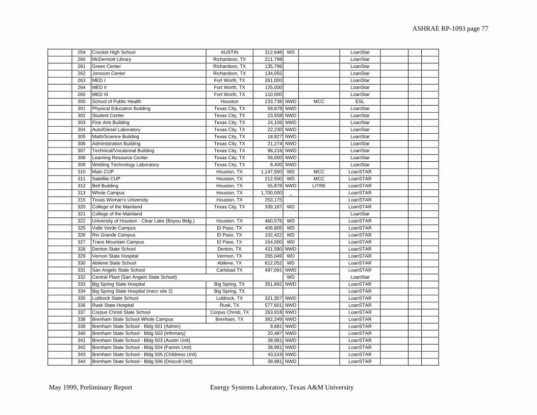
ASHRAE RP-1093 page 77
May 1999, Preliminary Report Energy Systems Laboratory, Texas A&M University
254 Crocket High School AUSTIN 312,648 WD LoanStar 260 McDermott Library Richardson, TX 211,798 LoanStar 261 Green Center Richardson, TX 135,796 LoanStar 262 Jonsson Center Richardson, TX 134,055 LoanStar 263 MED I Fort Worth, TX 261,000 LoanStar 264 MED II Fort Worth, TX 125,000 LoanStar 265 MED III Fort Worth, TX 110,000 LoanStar 300 School of Public Health Houston 233,738 NWD MCC ESL 301 Physical Education Building Texas City, TX 58,678 NWD LoanStar 302 Student Center Texas City, TX 23,558 NWD LoanStar 303 Fine Arts Building Texas City, TX 24,106 NWD LoanStar 304 Auto/Diesel Laboratory Texas City, TX 22,230 NWD LoanStar 305 Math/Science Building Texas City, TX 18,827 NWD LoanStar 306 Administration Building Texas City, TX 21,274 NWD LoanStar 307 Technical/Vocational Building Texas City, TX 96,216 NWD LoanStar 308 Learning Resource Center Texas City, TX 56,000 NWD LoanStar 309 Welding Technology Laboratory Texas City, TX 8,400 NWD LoanStar 310 Main CUP Houston, TX 1,147,500 WD MCC LoanSTAR 311 Satellite CUP Houston, TX 212,500 WD MCC LoanSTAR 312 Bell Building Houston, TX 55,878 NWD LITRE LoanSTAR 313 Whole Campus Houston, TX 1,700,000 _ LoanSTAR 315 Texas Woman's University Houston, TX 253,175 LoanSTAR 320 College of the Mainland Texas City, TX 339,167 WD LoanSTAR 321 College of the Mainland LoanStar 322 University of Houston - Clear Lake (Boyou Bldg.) Houston, TX 460,576 WD LoanSTAR 325 Valle Verde Campus El Paso, TX 406,805 WD LoanSTAR 326 Rio Grande Campus El Paso, TX 102,422 WD LoanSTAR 327 Trans Mountain Campus El Paso, TX 154,000 WD LoanSTAR 328 Denton State School Denton, TX 431,580 NWD LoanSTAR 329 Vernon State Hospital Vermon, TX 265,049 WD LoanSTAR 330 Abilene State School Abilene, TX 612,052 WD LoanSTAR 331 San Angelo State School Carlsbad TX 497,091 NWD LoanSTAR 332 Central Plant (San Angelo State School) WD LoanStar 333 Big Spring State Hospital Big Spring, TX 351,892 NWD LoanSTAR 334 Big Spring State Hospital (mecr site 2) Big Spring, TX LoanSTAR 335 Lubbock State School Lubbock, TX 321,357 NWD LoanSTAR 336 Rusk State Hospital Rusk, TX 577,601 NWD LoanSTAR 337 Corpus Christi State School Corpus Christi, TX 263,918 NWD LoanSTAR 338 Brenham State School Whole Campus Brenham, TX 362,249 NWD LoanSTAR 339 Brenham State School - Bldg 501 (Admin) 9,681 NWD LoanSTAR 340 Brenham State School - Bldg 502 (Infirmary) 20,487 NWD LoanSTAR 341 Brenham State School - Bldg 503 (Austin Unit) 38,981 NWD LoanSTAR 342 Brenham State School - Bldg 504 (Fannin Unit) 38,981 NWD LoanSTAR 343 Brenham State School - Bldg 505 (Childress Unit) 43,519 NWD LoanSTAR 344 Brenham State School - Bldg 506 (Driscoll Unit) 38,981 NWD LoanSTAR
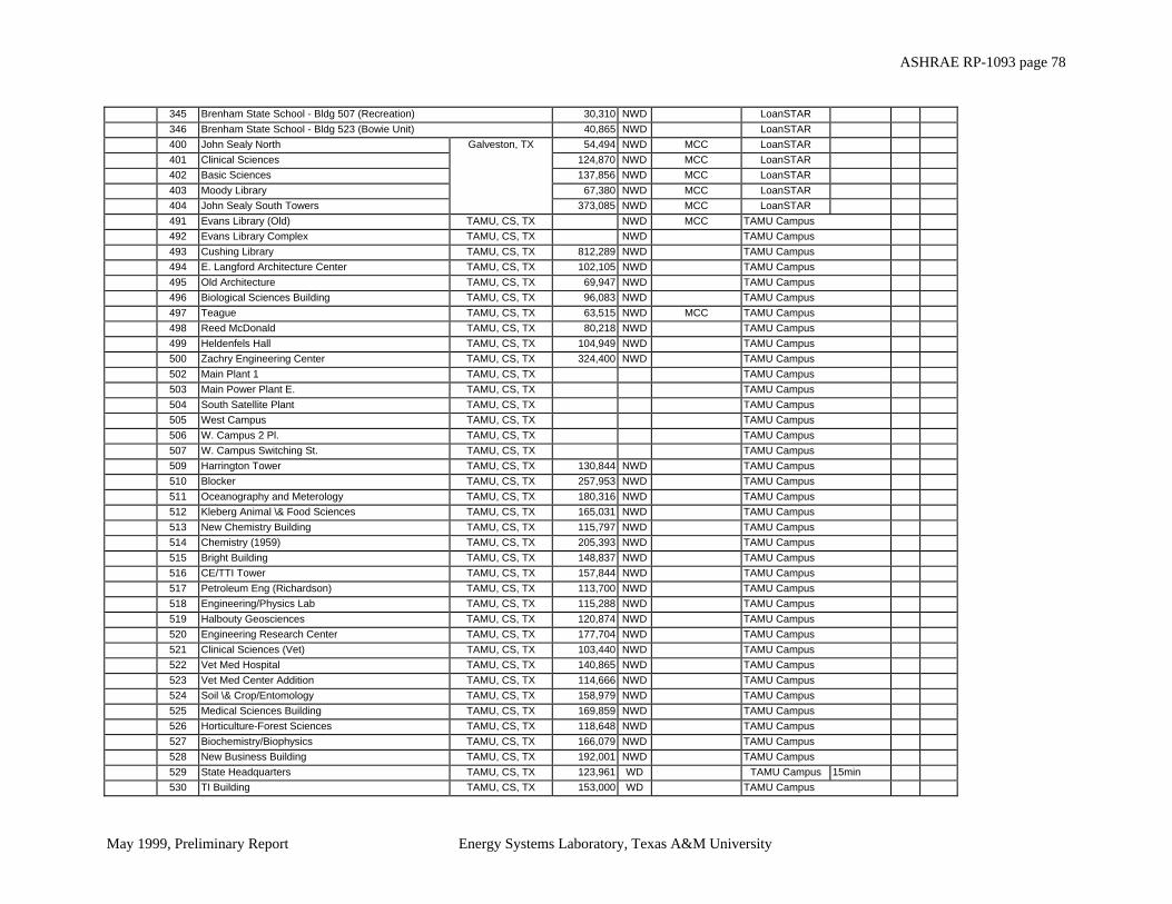
ASHRAE RP-1093 page 78
May 1999, Preliminary Report Energy Systems Laboratory, Texas A&M University
345 Brenham State School - Bldg 507 (Recreation) 30,310 NWD LoanSTAR 346 Brenham State School - Bldg 523 (Bowie Unit) 40,865 NWD LoanSTAR 400 John Sealy North Galveston, TX 54,494 NWD MCC LoanSTAR 401 Clinical Sciences 124,870 NWD MCC LoanSTAR 402 Basic Sciences 137,856 NWD MCC LoanSTAR 403 Moody Library 67,380 NWD MCC LoanSTAR 404 John Sealy South Towers 373,085 NWD MCC LoanSTAR 491 Evans Library (Old) TAMU, CS, TX NWD MCC TAMU Campus 492 Evans Library Complex TAMU, CS, TX NWD TAMU Campus 493 Cushing Library TAMU, CS, TX 812,289 NWD TAMU Campus 494 E. Langford Architecture Center TAMU, CS, TX 102,105 NWD TAMU Campus 495 Old Architecture TAMU, CS, TX 69,947 NWD TAMU Campus 496 Biological Sciences Building TAMU, CS, TX 96,083 NWD TAMU Campus 497 Teague TAMU, CS, TX 63,515 NWD MCC TAMU Campus 498 Reed McDonald TAMU, CS, TX 80,218 NWD TAMU Campus 499 Heldenfels Hall TAMU, CS, TX 104,949 NWD TAMU Campus 500 Zachry Engineering Center TAMU, CS, TX 324,400 NWD TAMU Campus 502 Main Plant 1 TAMU, CS, TX TAMU Campus 503 Main Power Plant E. TAMU, CS, TX TAMU Campus 504 South Satellite Plant TAMU, CS, TX TAMU Campus 505 West Campus TAMU, CS, TX TAMU Campus 506 W. Campus 2 Pl. TAMU, CS, TX TAMU Campus 507 W. Campus Switching St. TAMU, CS, TX TAMU Campus 509 Harrington Tower TAMU, CS, TX 130,844 NWD TAMU Campus 510 Blocker TAMU, CS, TX 257,953 NWD TAMU Campus 511 Oceanography and Meterology TAMU, CS, TX 180,316 NWD TAMU Campus 512 Kleberg Animal \& Food Sciences TAMU, CS, TX 165,031 NWD TAMU Campus 513 New Chemistry Building TAMU, CS, TX 115,797 NWD TAMU Campus 514 Chemistry (1959) TAMU, CS, TX 205,393 NWD TAMU Campus 515 Bright Building TAMU, CS, TX 148,837 NWD TAMU Campus 516 CE/TTI Tower TAMU, CS, TX 157,844 NWD TAMU Campus 517 Petroleum Eng (Richardson) TAMU, CS, TX 113,700 NWD TAMU Campus 518 Engineering/Physics Lab TAMU, CS, TX 115,288 NWD TAMU Campus 519 Halbouty Geosciences TAMU, CS, TX 120,874 NWD TAMU Campus 520 Engineering Research Center TAMU, CS, TX 177,704 NWD TAMU Campus 521 Clinical Sciences (Vet) TAMU, CS, TX 103,440 NWD TAMU Campus 522 Vet Med Hospital TAMU, CS, TX 140,865 NWD TAMU Campus 523 Vet Med Center Addition TAMU, CS, TX 114,666 NWD TAMU Campus 524 Soil \& Crop/Entomology TAMU, CS, TX 158,979 NWD TAMU Campus 525 Medical Sciences Building TAMU, CS, TX 169,859 NWD TAMU Campus 526 Horticulture-Forest Sciences TAMU, CS, TX 118,648 NWD TAMU Campus 527 Biochemistry/Biophysics TAMU, CS, TX 166,079 NWD TAMU Campus 528 New Business Building TAMU, CS, TX 192,001 NWD TAMU Campus 529 State Headquarters TAMU, CS, TX 123,961 WD TAMU Campus 15min 530 TI Building TAMU, CS, TX 153,000 WD TAMU Campus
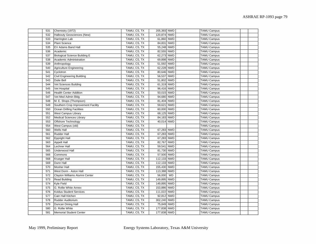
ASHRAE RP-1093 page 79
May 1999, Preliminary Report Energy Systems Laboratory, Texas A&M University
531 Chemistry (1972) TAMU, CS, TX 205,393 NWD TAMU Campus 532 Halbouty Geosciences (New) TAMU, CS, TX 120,874 NWD TAMU Campus 533 Harrington Lab TAMU, CS, TX 61,860 NWD TAMU Campus 534 Plant Science TAMU, CS, TX 84,831 NWD TAMU Campus 535 EV Adams Band Hall TAMU, CS, TX 55,248 NWD TAMU Campus 536 Academic TAMU, CS, TX 82,555 NWD TAMU Campus 537 Biological Science Building E TAMU, CS, TX 62,273 NWD TAMU Campus 538 Academic Administration TAMU, CS, TX 69,898 NWD TAMU Campus 539 Anthropology TAMU, CS, TX 51,592 NWD TAMU Campus 540 Agriculture Engineering TAMU, CS, TX 62,228 NWD TAMU Campus 541 Cyclotron TAMU, CS, TX 80,646 NWD TAMU Campus 542 Civil Engineering Building TAMU, CS, TX 56,537 NWD TAMU Campus 543 Dulie Bell TAMU, CS, TX 51,802 NWD TAMU Campus 544 Vet Sciences Building TAMU, CS, TX 61,319 NWD TAMU Campus 545 Vet Hospital TAMU, CS, TX 96,416 NWD TAMU Campus 546 Health Center Addition TAMU, CS, TX 50,015 NWD TAMU Campus 547 Vet Med Admin Bldg TAMU, CS, TX 94,680 NWD TAMU Campus 548 M. E. Shops (Thompson) TAMU, CS, TX 81,404 NWD TAMU Campus 549 Southern Crop Improvement Facility TAMU, CS, TX 59,621 NWD TAMU Campus 550 Ocean Drilling Facilities TAMU, CS, TX 60,000 NWD TAMU Campus 551 West Campus Library TAMU, CS, TX 68,125 NWD TAMU Campus 552 Medical Sciences Library TAMU, CS, TX 84,183 NWD TAMU Campus 553 Offshore Technology TAMU, CS, TX 40,014 NWD TAMU Campus 554 West Campus (old) TAMU, CS, TX TAMU Campus 560 Wells Hall TAMU, CS, TX 67,283 NWD TAMU Campus 561 Rudder Hall TAMU, CS, TX 67,283 NWD TAMU Campus 562 Eppright Hall TAMU, CS, TX 67,283 NWD TAMU Campus 563 Appelt Hall TAMU, CS, TX 82,767 NWD TAMU Campus 564 Lechner Hall TAMU, CS, TX 59,541 NWD TAMU Campus 565 Underwood Hall TAMU, CS, TX 81,730 NWD TAMU Campus 566 Commons TAMU, CS, TX 57,500 NWD TAMU Campus 568 Krueger Hall TAMU, CS, TX 112,133 NWD TAMU Campus 569 Dunn Hall TAMU, CS, TX 112,133 NWD TAMU Campus 570 Mosher Hall TAMU, CS, TX 155,430 NWD TAMU Campus 571 West Dorm - Aston Hall TAMU, CS, TX 113,388 NWD TAMU Campus 572 Clayton Williams Alumni Center TAMU, CS, TX 56,000 WD TAMU Campus 573 Read Building TAMU, CS, TX 149,895 NWD TAMU Campus 574 Kyle Field TAMU, CS, TX 149,895 NWD TAMU Campus 575 G. Rollie White Annex TAMU, CS, TX 153,886 NWD TAMU Campus 576 Koldus Student Services TAMU, CS, TX 111,022 NWD TAMU Campus 577 Cain Hall Kitchen TAMU, CS, TX 92,812 NWD TAMU Campus 578 Rudder Auditorium TAMU, CS, TX 302,240 NWD TAMU Campus 579 Duncan Dining Hall TAMU, CS, TX 75,849 NWD TAMU Campus 580 G. Rollie White TAMU, CS, TX 177,838 NWD TAMU Campus 581 Memorial Student Center TAMU, CS, TX 177,838 NWD TAMU Campus

ASHRAE RP-1093 page 80
May 1999, Preliminary Report Energy Systems Laboratory, Texas A&M University
582 MSC Annex TAMU, CS, TX 368,935 NWD TAMU Campus 583 Sbisa Dining Hall TAMU, CS, TX 137,913 NWD TAMU Campus 586 Clements Hall TAMU, CS, TX 62,156 NWD TAMU Campus 587 Haas Hall TAMU, CS, TX 69,668 NWD TAMU Campus 588 McFadden Hall TAMU, CS, TX 62,156 NWD TAMU Campus 589 Neely Hall TAMU, CS, TX 69,668 NWD TAMU Campus 590 Hobby Hall TAMU, CS, TX 62,156 NWD TAMU Campus 591 McKenzie Terminal TAMU, CS, TX 32,188 WD TAMU Campus 593 Recreational Sports \& Natorium TAMU, CS, TX 289,000 NWD TAMU Campus 599 A&M westinghouse data TAMU, CS, TX NA NA 601 Torres Unit Huntsville, TX NA NA 602 Boyd Unit Huntsville, TX NA NA 604 Stevesson Unit Huntsville, TX NA NA 605 Brisco Unit Huntsville, TX NA NA 606 Lynaugh Unit Huntsville, TX NA NA 607 Smith Unit Huntsville, TX NA NA 608 Wallace Unit Huntsville, TX NA NA 609 Roach Unit Huntsville, TX NA NA 610 Neal Unit Huntsville, TX NA NA 611 Jordan Unit Huntsville, TX NA NA 612 Dalhart Unit Huntsville, TX NA NA 701 Power Plant Chillers Capitol Complex 42,116 WD Minnesota 702 Power Plant WD 703 Administration Bldg. Capitol Complex 80,000 WD Minnesota 704 Judicial Building Capitol Complex 200,829 NWD Minnesota 705 Health Building Capitol Complex 197,260 WD Minnesota 706 Ford Building Capitol Complex 57,047 NWD Minnesota 707 State Office Bldg. Capitol Complex 281,850 NWD Minnesota 708 Dept. of Transportation Bldg. Capitol Complex 378,100 NWD Minnesota 709 Veterans Building Capitol Complex 87,664 NWD Minnesota 710 Capitol Building Capitol Complex 366,805 NWD Minnesota 711 Centennial Building Capitol Complex 317,286 NWD Minnesota 712 Criminal Apprehension Bldg. Capitol Complex 77,630 NWD Minnesota 713 Capitol Square Building Capitol Complex 225,479 WD Minnesota 714 Somsen Hall Winona S U, MN 176,221 WD Minnesota 715 Phelps Hall Winona S U, MN 41,058 NWD Minnesota 716 Pasteur Hall Winona S U, MN 60,752 NWD Minnesota 717 Kryzsko Building Winona S U, MN 108,825 NWD Minnesota 718 Whole Campus Winona S U, MN 1,263,428 Minnesota 719 Lourdes Hall Winona S U, MN 50,000 NWD Minnesota 721 Howell Hall Winona S U, MN 23,117 NWD Minnesota 722 Prentiss Hall Winona S U, MN 45,503 NWD Minnesota 723 Memorial Hall Winona S U, MN 142,241 NWD Minnesota 724 Performance Art Center Winona S U, MN 86,291 NWD Minnesota 725 Maxwell Library Winona S U, MN 87,567 NWD Minnesota
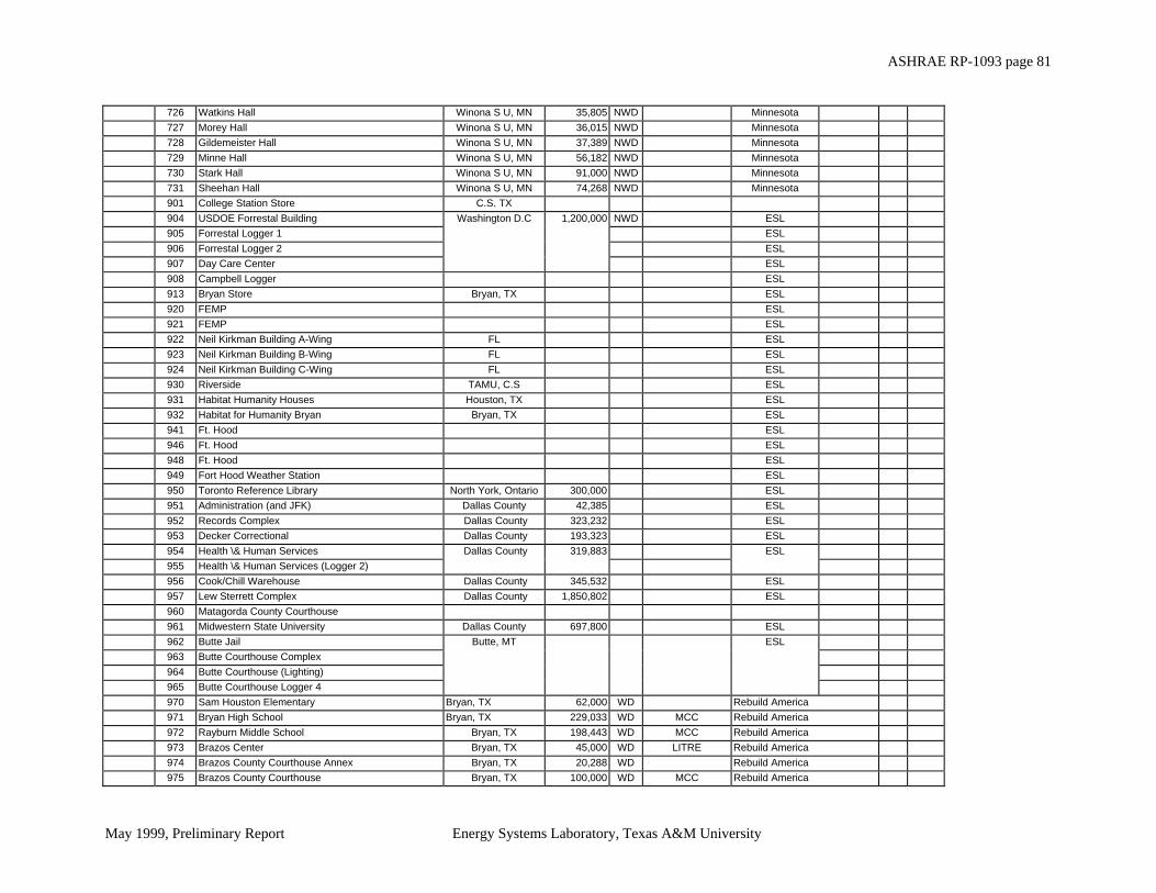
ASHRAE RP-1093 page 81
May 1999, Preliminary Report Energy Systems Laboratory, Texas A&M University
726 Watkins Hall Winona S U, MN 35,805 NWD Minnesota 727 Morey Hall Winona S U, MN 36,015 NWD Minnesota 728 Gildemeister Hall Winona S U, MN 37,389 NWD Minnesota 729 Minne Hall Winona S U, MN 56,182 NWD Minnesota 730 Stark Hall Winona S U, MN 91,000 NWD Minnesota 731 Sheehan Hall Winona S U, MN 74,268 NWD Minnesota 901 College Station Store C.S. TX 904 USDOE Forrestal Building Washington D.C 1,200,000 NWD ESL 905 Forrestal Logger 1 ESL 906 Forrestal Logger 2 ESL 907 Day Care Center ESL 908 Campbell Logger ESL 913 Bryan Store Bryan, TX ESL 920 FEMP ESL 921 FEMP ESL 922 Neil Kirkman Building A-Wing FL ESL 923 Neil Kirkman Building B-Wing FL ESL 924 Neil Kirkman Building C-Wing FL ESL 930 Riverside TAMU, C.S ESL 931 Habitat Humanity Houses Houston, TX ESL 932 Habitat for Humanity Bryan Bryan, TX ESL 941 Ft. Hood ESL 946 Ft. Hood ESL 948 Ft. Hood ESL 949 Fort Hood Weather Station ESL 950 Toronto Reference Library North York, Ontario 300,000 ESL 951 Administration (and JFK) Dallas County 42,385 ESL 952 Records Complex Dallas County 323,232 ESL 953 Decker Correctional Dallas County 193,323 ESL 954 Health \& Human Services Dallas County 319,883 ESL 955 Health \& Human Services (Logger 2) 956 Cook/Chill Warehouse Dallas County 345,532 ESL 957 Lew Sterrett Complex Dallas County 1,850,802 ESL 960 Matagorda County Courthouse 961 Midwestern State University Dallas County 697,800 ESL 962 Butte Jail Butte, MT ESL 963 Butte Courthouse Complex 964 Butte Courthouse (Lighting) 965 Butte Courthouse Logger 4 970 Sam Houston Elementary Bryan, TX 62,000 WD Rebuild America 971 Bryan High School Bryan, TX 229,033 WD MCC Rebuild America 972 Rayburn Middle School Bryan, TX 198,443 WD MCC Rebuild America 973 Brazos Center Bryan, TX 45,000 WD LITRE Rebuild America 974 Brazos County Courthouse Annex Bryan, TX 20,288 WD Rebuild America 975 Brazos County Courthouse Bryan, TX 100,000 WD MCC Rebuild America

ASHRAE RP-1093 page 82
May 1999, Preliminary Report Energy Systems Laboratory, Texas A&M University
980 St Paul Place Dallas, TX 100,000 WD ESL 981 Harwood Center Dallas, TX 750,000 WD ESL 982 9700 Richmond Dallas, TX 89,000 WD ESL 983 3300 Gessner Dallas, TX 65,500 WD ESL 984 McKinney Place Dallas, TX 100,000 MCC ESL 985 Pittman Atrium Dallas, TX 100,000 WD MCC ESL 986 Brooke Army Medical Center Fort Sam Houston 1,200,000 WD ESL 15 min Legend: WBE Measured Whole Building Electricity Consumption NWD for buildings without Chillers WD for buildings with Chillers L&R Measured Lights and Receptacles WBE-MCC L&R derived from the difference between measured Whole Building Electricity and Motor Control Center (Pumps) Consumptions LIGHT Measured Lighting consumption LITEQ Measured Lighting and Equipment consumption EQUIP Measured Equipment consumption
Table 8. All buildings monitored by ESL

ASHRAE RP-1093 page 83
May 1999, Preliminary Report Energy Systems Laboratory, Texas A&M University
List of contacts who provided us with positive responses in terms of availability of metered commercial building end-uses in their organizations
From Europe: 0. Jean Lebrun
Professor Laboratoire de Thermodynamique Universite de Liege, Campus du Sart Tilman, Batiment B49, Parking P33 B4000 Liege, Belgium Phone: +32 4 366 48 01 Fax: +32 4 366 48 12 Email: [email protected] Web: http://www.ulg.ac.be/labothap
1. Casper Kofod DEFU Denmark Email: [email protected]
2. Guislain Burle
MD3E SA Manager France Email: [email protected]
From the U.S.: 0. Mimi Goldberg
Xenergy 2001 West Beltine Highway, Suite 200 Madison, WI 53713 Phone: (608) 277-9696 FAX: (608) 277-9690 Email: [email protected]
1. Jim Halpern
President Measuring & Monitoring Services 620 Shrewsbury Avenue Tinton Falls, NJ 07701 Phone: (732) 530-3280

ASHRAE RP-1093 page 84
May 1999, Preliminary Report Energy Systems Laboratory, Texas A&M University
Fax: (732) 576-8067 Email: [email protected]
2. Ilene Obstfeld
EPRI-CEED Phone: (503) 768-4680 Email: [email protected]
3. John Farley EPRI-CEED Vice President EPS Solutions One Richmond Square, Suite 122C Providence, Rhode Island 02906 Phone: (401) 621-2240 Fax: (401) 621-2260 Email: [email protected]
4. Z. Todd Taylor
Research Engineer Energy Sciences Department Battelle PNNL Battelle Boulevard Richland, WA 99352 Phone: (509) 375-2676 Fax: (509) 375-3614
5. Maryanne Piette
Environmental Energy Technologies Division 90-2074 Lawrence Berkeley Laboratory University of California 1 Cyclotron Road Berkeley, CA 94720 Phone: (415) 486-6286 Fax: (415) 486-4673 Email: [email protected]
6. John McBride
President NCAT Development Corporation P.O. 5000 Butte, MT 59702 Phone: (406) 494-4572 Fax: (406) 494-2905

ASHRAE RP-1093 page 85
May 1999, Preliminary Report Energy Systems Laboratory, Texas A&M University
7. Taghi Alereza ADM & Associates 3299 Ramos Circle Sacramento, CA 95827 Phone: (916) 363-8383 Fax: (916) 363-1788