r bulletin 107 — august 2001

42

ESCOUBET 24-08-2001 13:29 Page 2

Rumba, Salsa, Samba and Tango in theMagnetosphere- The Cluster Quartet’s First Year in Space

C.P. Escoubet & M. FehringerSolar System Division, Space Science Department, ESA Directorate of ScientificProgrammes, Noordwijk, The Netherlands

P. BondCranleigh, Surrey, United Kingdom

IntroductionCluster is one of the two missions – the otherbeing the Solar and Heliospheric Observatory(SOHO) – constituting the Solar TerrestrialScience Programme (STSP), the first‘Cornerstone’ of ESA’s Horizon 2000Programme. The Cluster mission was firstproposed in November 1982 in response to anESA Call for Proposals for the next series ofscientific missions.

Launch and commissioning phaseWhen the first Soyuz blasted off from theBaikonur Cosmodrome on 16 July 2000, weknew that Cluster was well on the way torecovery from the previous launch setback.However, it was not until the second launch on9 August 2000 and the proper injection of thesecond pair of spacecraft into orbit that weknew that the Cluster mission was truly backon track (Fig. 1). In fact, the experimenters saidthat they knew they had an ideal mission onlyafter switching on their last instruments on thefourth spacecraft.

After the two launches, a quite lengthyverification phase for all spacecraft subsystemsand the payload of 44 instruments (Table 1)started. The 16 solid booms, eight for themagnetometers and eight for communications,were successfully deployed. A few days later,the spacecraft had to survive the first longeclipses, with up to 4 h of darkness, which theydid with very good performances from theonboard batteries.

Then started the verification phase for the 11 sets of instruments. This phase wascomplicated by the fact that, to perform theirmeasurements, some instruments had todeploy very long wire antennas. These 44 mantennas altered the spin rate of thespacecraft, which was incompatible with theparticle instruments that needed a fixed spinrate. Altogether, more than 1100 individualtasks were performed on the instruments. At the end of this phase, in early December, a two-week ‘interference campaign’ wasconducted to test how much the instrumentsinfluenced each other. After successfully testingall the instruments, the nominal operationsphase began on 1 February 2001. Some of theresults that are presented below were obtainedduring the commissioning and verification phase.

The four Cluster spacecraft were successfully launched in pairs bytwo Russian Soyuz rockets on 16 July and 9 August 2000. On 14August, the second pair joined the first pair in highly eccentric polarorbits, with an apogee of 19.6 Earth radii and a perigee of 4 Earth radii.The very accurate orbital injection and low fuel consumption meanthat spacecraft operations could continue for at least two more yearsafter the nominal two-year mission.

This is the first time that the Earth’s magnetic field and its environmenthave been explored by a small constellation of four identicalspacecraft. Preliminary results show that, as predicted, with fourspacecraft we can obtain a detailed three-dimensional view of theSun-Earth connection processes taking place at the interfacebetween the solar wind and the Earth’s magnetic field.

the cluster quartet’s first year in space

After the Ariane-5 launcher failure on 4 June1996 and the destruction of the four originalCluster spacecraft, the Cluster scientistsconvinced the ESA Science ProgrammeCommittee (SPC) that it was essential for theEuropean scientific community to rebuild themission. This was agreed by the SPC in April1997. In the meantime, SOHO, launched inDecember 1995, had begun to make somevery exciting discoveries about the Sun and itsenvironment. Now, with the successful launchof the rebuilt Cluster satellites, the STSPCornerstone is complete and it is possible tocombine these two missions in order to studythe full chain of processes from the Sun’sinterior to the Earth.

43

ESCOUBET 24-08-2001 13:29 Page 3

Figure 1. The two launchesof the Cluster spacecraft on

two Soyuz-Fregat rockets,on 16 July and 9 August

2000. An onboard cameratook 27 pictures when

Rumba-SC1 separated fromTango-SC4. Tango is shown

in the upper-right corner.The Earth can be seen in

the background

The Earth’s magnetosphere is a very largevolume of space extending about 65 000 km inthe Sun’s direction, and more than two million kmin the opposite direction. The Earth’s magneticfield dominates this space. Without thecontinuous flow of plasma (electrically chargedparticles) from the Sun, the Earth’s magneticfield would be a dipole with a symmetricmagnetic field around the polar axis. Instead,the solar wind compresses the magnetosphereon the front side and shapes it into a long tail inthe anti-sunward direction (Fig. 2). During thefirst months of operations, the spacecraft orbitsallowed Cluster to visit key regions of themagnetosphere – the bow shock, the

r bulletin 107 — august 2001

44

Table 1. The 11 instruments on each of the four Cluster spacecraft

Instrument Principal Investigator

ASPOC (Spacecraft potential control) K. Torkar (IWF, A)

CIS (Ion composition) H. Rème (CESR, F)

EDI (Plasma drift velocity) G. Paschmann (MPE, D)

FGM (Magnetometer) A. Balogh (IC, UK)

PEACE (Electrons) A. Fazakerley (MSSL, UK)

RAPID (High-energy electrons and ions) P. Daly (MPAe, D)

DWP * (Wave processor) H. Alleyne (Sheffield, UK)

EFW * (Electric field and waves) M. André (IRFU, S)

STAFF * (Magnetic and electric fluctuations) N. Cornilleau (CETP, F)

WBD * (Electric field and wave forms) D. Gurnett (IOWA, USA)

WHISPER * (Electron density and waves) P. Décréau (LPCE, F)

* Wave Experiment Consortium (WEC)

magnetopause and the polar cusp. In addition,unique data were obtained during a strongsolar storm that occurred in November 2000.

The bow shockThe bow shock is the surface that forms in frontof the Earth’s magnetosphere when thesupersonic solar wind slams into it at a speedof about 400 km/s (around 1.5 million km/h).This is similar to the shock wave (or sonicboom) when a plane flies faster than the speedof sound in the atmosphere. The bow shockslows down the solar wind and deflects itaround the magnetosphere. In the process, theparticles – electron and ions – are heated andthe strength of the magnetic field is increased.Intense electromagnetic waves are alsoproduced at the shock.

Figure 3 shows the electric waves detected bythe WHISPER instrument during two crossingsof the bow shock by the four Clusterspacecraft. On the plot, which covers a periodof 40 minutes, the wave frequency is shown asa function of time. The power of the waves isplotted in false colours: red/brown for the mostintense and blue for the less intense.

The bow shock is characterised by an intensewave-emission enhancement below 20 kHzthat is observed around 08:25 and 08:35 UT.The crossings do not occur at the same timefor all spacecraft due to their different positions,which were about 600 km from each other atthat time. The right panel of Figure 3 shows thespacecraft configuration at the first crossing,when they were located on the right flank of thebow shock. A closer view of the spacecraftconfiguration is shown in the middle-right andbottom-right panels.

16 July 2000

9 August 2000

SC4 and SC1 separation

ESCOUBET 24-08-2001 13:29 Page 4

the cluster quartet’s first year in space

45

Figure 2. The Cluster orbitand the regions crossedduring the first phase of themission

Figure 3. Bow-shockcrossings by each of the four Cluster spacecraft on 22 December 2000. The left panels show thefrequency/time spectrogramsof the electric wavesobserved by the WHISPERinstrument. Between about08:25 and 08:35 UT, thespacecraft were in the solarwind. The diagrams on theright show the Clusterconfiguration during thebow-shock crossing, in anoverall view (upper panel)and two enlarged views at08:23 UT (middle panel) and08:27 UT (bottom panel). The spacecraft and theirtrajectories are colour-coded:spacecraft 1 (Rumba-SC1) isshown in black, Salsa-SC2 in red, Samba-SC3 in green,and Tango-SC4 in magenta.Data courtesy of WHISPERPrincipal Investigator, P. Décréau (LPCE, France)

Sign

al le

vel (

dB0)

Fp(kHz)

50

60

40

20

0

20

50

20

50

20

50

20

80

40

08:05 08:15Universal Time (HH:MM)

Solar wind

Magnetosheath

08:25 08:35 08:45

Ne

(cm

-3)

ESCOUBET 24-08-2001 13:30 Page 5

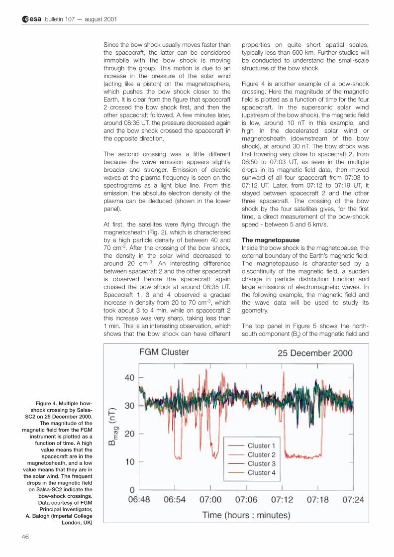
Figure 4. Multiple bow-shock crossing by Salsa-

SC2 on 25 December 2000.The magnitude of the

magnetic field from the FGMinstrument is plotted as a

function of time. A highvalue means that thespacecraft are in the

magnetosheath, and a lowvalue means that they are inthe solar wind. The frequent

drops in the magnetic fieldon Salsa-SC2 indicate the

bow-shock crossings.Data courtesy of FGMPrincipal Investigator,

A. Balogh (Imperial CollegeLondon, UK)

Since the bow shock usually moves faster thanthe spacecraft, the latter can be consideredimmobile with the bow shock is movingthrough the group. This motion is due to anincrease in the pressure of the solar wind(acting like a piston) on the magnetosphere,which pushes the bow shock closer to theEarth. It is clear from the figure that spacecraft2 crossed the bow shock first, and then theother spacecraft followed. A few minutes later,around 08:35 UT, the pressure decreased againand the bow shock crossed the spacecraft inthe opposite direction.

The second crossing was a little differentbecause the wave emission appears slightlybroader and stronger. Emission of electricwaves at the plasma frequency is seen on thespectrograms as a light blue line. From thisemission, the absolute electron density of theplasma can be deduced (shown in the lowerpanel).

At first, the satellites were flying through themagnetosheath (Fig. 2), which is characterisedby a high particle density of between 40 and 70 cm-3. After the crossing of the bow shock,the density in the solar wind decreased toaround 20 cm-3. An interesting differencebetween spacecraft 2 and the other spacecraftis observed before the spacecraft againcrossed the bow shock at around 08:35 UT.Spacecraft 1, 3 and 4 observed a gradualincrease in density from 20 to 70 cm-3, whichtook about 3 to 4 min, while on spacecraft 2this increase was very sharp, taking less than 1 min. This is an interesting observation, whichshows that the bow shock can have different

properties on quite short spatial scales,typically less than 600 km. Further studies willbe conducted to understand the small-scalestructures of the bow shock.

Figure 4 is another example of a bow-shockcrossing. Here the magnitude of the magneticfield is plotted as a function of time for the fourspacecraft. In the supersonic solar wind(upstream of the bow shock), the magnetic fieldis low, around 10 nT in this example, and high in the decelerated solar wind ormagnetosheath (downstream of the bowshock), at around 30 nT. The bow shock wasfirst hovering very close to spacecraft 2, from06:50 to 07:03 UT, as seen in the multipledrops in its magnetic-field data, then movedsunward of all four spacecraft from 07:03 to07:12 UT. Later, from 07:12 to 07:19 UT, itstayed between spacecraft 2 and the otherthree spacecraft. The crossing of the bowshock by the four satellites gives, for the firsttime, a direct measurement of the bow-shockspeed - between 5 and 6 km/s.

The magnetopauseInside the bow shock is the magnetopause, theexternal boundary of the Earth’s magnetic field.The magnetopause is characterised by adiscontinuity of the magnetic field, a suddenchange in particle distribution function andlarge emissions of electromagnetic waves. Inthe following example, the magnetic field andthe wave data will be used to study itsgeometry.

The top panel in Figure 5 shows the north-south component (Bz) of the magnetic field and

r bulletin 107 — august 2001

46

ESCOUBET 24-08-2001 13:30 Page 6

Figure 5. Magnetopausecrossing by the fourspacecraft on 10 December2000. The Bz component ofthe magnetic field is plottedas a function of time (highvalue means inside themagnetosphere, and lowvalue means outside). Inaddition, the integratedwave power from the STAFFinstrument is plotted as afunction of time. Themaximum in the wave power(marked at the bottom by an arrow) indicates themagnetopause crossing.The diagram at the bottomshows the magnetopausesurface and its normal planedetected by the fourspacecraft. A wave passingby the spacecraft is shownin red.Data courtesy of STAFFPrincipal Investigator, N. Cornilleau-Wehrlin (CETP,France), and FGM PrincipalInvestigator, A. Balogh(Imperial College London,UK)

panel). Given their location at the outerboundary of the magnetosphere, the polarcusps react rapidly to changes that occur in thesolar wind. For instance, when the solar windchanges from a north- to a south-pointingmagnetic field, the cusp moves to lowerlatitudinal positions. On the other hand, whenthe solar-wind magnetic field changes to anazimuthal direction, the polar cusp moveslongitudinally. The motion of the cusp is,therefore, a key element in the Sun – Earthinteraction.

Until now, the polar cusp had only beenobserved by single spacecraft, so its motioncould only be deduced indirectly from statisticalanalysis by combining many crossings. WithCluster, four spacecraft are visiting this regionfor the first time, allowing the speed of the polarcusp to be measured directly.

the cluster quartet’s first year in space

47

the total emission power of the magnetic wavesgenerated around the magnetopause. Themagnetopause is defined by the maximumpower of the waves corresponding to thechange in sign of Bz. The arrows at the bottomof the plot show the exact time of themagnetopause crossing. It is interesting to notethat spacecraft 1 crossed the magnetopausefirst, then spacecraft 2 and 4 at the same time,and finally spacecraft 3.

Using a minimum-variance analysis, whichmeans looking for a system where thevariations in B are minimal, the magnetopauseplane can be defined for each spacecraftcrossing. The result is shown in the bottompanel of Figure 5. The individual spacecraftpositions as well as the magnetopause planeare shown. It is clear that spacecraft 1, 3 and 4detected the magnetopause in approximatelythe same plane, while spacecraft 2 detected it in an almost perpendicular plane. Thisobservation cannot be explained by a usualplanar magnetopause surface, but instead by awave propagating along the magnetopause.The speed of this wave has been estimated ataround 70 km/s. A simulation of this wave isshown in Figure 6. It is clear from this examplethat all four spacecraft are needed to measurethe three-dimensional properties of themagnetopause. With two or three spacecraft,we could have missed the wave.

The polar cuspThe polar cusp is the ‘window’ above thenorthern and southern polar regions where theparticles from the solar wind can penetratedirectly into the magnetosphere (Fig. 7, top

ESCOUBET 24-08-2001 13:30 Page 7

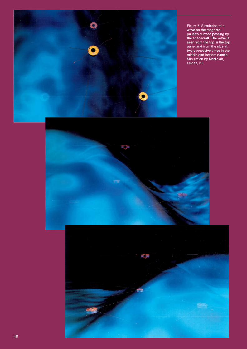
Figure 6. Simulation of awave on the magneto-pause’s surface passing bythe spacecraft. The wave isseen from the top in the toppanel and from the side attwo successive times in themiddle and bottom panels.Simulation by Medialab,Leiden, NL

48

ESCOUBET 24-08-2001 13:30 Page 8

the cluster quartet’s first year in space

49

Figure 7. Cusp crossing on14 January 2001. Top panel:sketch of the polar cuspwith the four spacecraft.Bottom panel: energy/timespectrograms of ions fromRumba-SC1, Samba-SC3and Tango-SC4. The totalion density is also plotted in the panel above eachspectrogram.Data courtesy of CISPrincipal Investigator H. Rème and Co-Investigator J.P. Bosqued(CESR, France)

ESCOUBET 24-08-2001 13:31 Page 9

Figure 8. Ground-basedradar observations on

14 January 2001. The leftpanel shows the projection

of the Cluster trajectory overthe northern polar cap. Thefields of view of the Eiscat(red) and Superdarn (grey)radars are indicated. The

right panels show theplasma convection patternrecorded by Superdarn at

13:20 UT (top) and at 13:30UT (bottom). An

enhancement of the flowtowards the east is detected

at 13:30 (yellow bright spotin the centre of the figure).

Data courtesy of H. Opgenoorth (Uppsala,

Sweden), M. Lockwood(RAL, UK) and R. Greenwald

(APL, USA).

The bottom panel in Figure 7 shows the datafrom the ion detectors on spacecraft 1, 3 and 4in the cusp region. The spacecraft were movingfrom above the pole at around 09:00 UT to the magnetosheath after 15:00 UT (Fig. 2). Inbetween these two regions, the spacecraftcrossed the polar cusp for about 30 minutes ataround 13:30 UT. A few other shorter crossingsof the polar cusp are also visible before andafter that time.

The polar cusp is characterised by ions, mainlyH+ and He++ of solar origin, with energiesbetween 100 eV and a few keV. On the largetime scale shown in this figure, all spacecraftshow the same data. However, as we will seebelow, clear differences are visible if we look atmore detailed data. The top panel in Figure 7sketches the spacecraft entering the polarcusp. Two spacecraft are in the cusp, one is atthe border, and the fourth one is still outside.The precise timing of the crossing by eachspacecraft and the spacecraft position will givethe speed of the cusp.

This crossing on 14 January 2001 wassupported by ground-based data sets, as theEiscat and Superdarn radars were just belowthe spacecraft and providing additionalinformation on the cusp region (Fig. 8). In fact,

just before the cusp crossing by Cluster, theradar detected a change in ionosphericconvection, which was an indication that thecusp was moving towards the east (bottom-right panel). This motion is sketched in Figure 9.

The left panel is a view from the Sun and showsthe motion of the cusp towards the Clusterposition (blue dot). The right panel shows theelectron data for one of these cusp crossingsby the four spacecraft. The entry of the spacecraftinto the cusp is marked by a red arrow and theexit by a white arrow. It is clear that the entryand exit do not occur at the same time for eachspacecraft. Using the time of the crossing andthe position of the spacecraft, we can estimatethat the polar cusp was moving at between 10and 30 km/s. This is the first time that thespeed of the cusp has been measured directly.

Solar storm in November 2000With the Sun now at maximum activity in its 11-year cycle, numerous powerful solar storms areexpected to occur. On 8 November 2000, thefourth biggest storm since 1976 was detectedby SOHO. A huge cloud of plasma, in the formof a Coronal Mass Ejection (CME), was directedtowards the Earth (Fig. 10). About 8 min later,the WHISPER instrument on Cluster detectedthe first consequence of the storm – an intense

r bulletin 107 — august 2001

50

ESCOUBET 24-08-2001 13:31 Page 10

In fact, single-event upsets, due to bit flips inthe solid-state memory, were detected on-board Cluster about 100 times more often thanunder normal conditions. The last manifestationof the storm, which occurred about 1 day later,was the arrival of the CME. This acted as apiston on the magnetosphere and reduced itssize by half.

radio emission from 20 kHz to above 80 kHz.Then, about 20 min later, the first energeticprotons accelerated during the storm arrived atthe Earth (Fig. 11). Their flux was 100 000 timeshigher than during quiet conditions.

These particles penetrate spacecraft andinstruments and may damage vital components.

the cluster quartet’s first year in space

51

Figure 9. Detailed dataobtained during the cuspcrossing on 14 January 2001.The left panel sketches themotion of the cusp towardsCluster, which enabled thespacecraft to enter the cuspunexpectedly. The rightpanels show the energy/timespectrograms of the electronpopulation observed by thefour spacecraft. The redarrows indicate when thespacecraft entered the cusp,and the white arrows whenthey left the cusp.Data courtesy of PEACEPrincipal Investigator, A. Fazakerley (MSSL, UK)

Figure 10. Solar storm on 8 - 10 November 2000. TheSOHO image taken on 8 November is shown in theupper left panel. The positionof Cluster is shown in theupper-right diagram. Thefrequency/time spectrogramsshowing the electric fieldwave measurements areshown at the bottom. Thelarge band emission (from 20 to more than 80 kHz) isobserved on Samba-SC3about 8 min after the stormstarted on the Sun. Data courtesy of WHISPERPrincipal Investigator, P. Décréau (LPCE, France)

Polarcusp

Polar cusp

Cluster

Normal position

Eastward shift

xy

80

60

40

20

Freq

ency

(kH

z)

Sign

al L

evel

(dB

)

2

21:30 22:00 22:30 23:00 23:30 00:00 00:30

7155

50

45

40

35

30

25

20

15

10

5

0

Universal Time

ESCOUBET 24-08-2001 13:31 Page 11

Figure 11. Protons producedduring the solar storm on

8 November 2000. The fluxis plotted for different

proton energies, from above10 MeV to above 100 MeV.

The protons were stillreaching the Earth, although

with decreasing fluxes,several days later.

Data courtesy of NOAA/SECBoulder, USA

When we received the early warning fromSOHO that the storm was coming, we decidedto record data for about one day on eachCluster spacecraft. Although not all instrumentswere operating at that time due to on-goingcommissioning activities, the FGM magneto-meter was switched on and so it was able todetect Cluster’s first excursion outside themagnetosphere.

Figure 12 shows the magnetohydrodynamic(MHD) model that simulates the magneto-sphere’s status during the storm. This modelreproduces the global interaction of the solarwind with the magnetosphere. All key physicalparameters - magnetic field, density andtemperature - are calculated in three dimensionsusing solar-wind data measured by the Windspacecraft upstream of the bow shock. In thetop panel, the magnetosphere is shown in darkblue, while to the left the magnetosheath isshown in green/yellow, and further to the leftthe solar wind is in light blue.

Due to the increased pressure coming from thesolar wind at 07:00 UT, the colours of theabove regions changed slightly, the solar windbecoming light yellow and the magnetosheathbecoming red. Before the arrival of the cloud, at05:48 UT, the magnetosphere was normal (toppanel) and Cluster was located inside it. Afterthe CME’s arrival (bottom panel), themagnetosphere was compressed to about halfof its normal size, and Cluster passed outside itand into the solar wind for many hours. Thiswas about 10 days earlier than expected by themission team.

Figure 13 shows the magnetometer data fromone excursion outside the magnetosphere

r bulletin 107 — august 2001

52

Figure 12.Magnetohydrodynamic

(MHD) model of themagnetosphere on

10 November 2000. The top panel shows the

magnetosphere before thearrival of the CME at 05:48

UT, and the bottom panelafter the arrival of the CME

at 07:00 UT.Data courtesy of J. Berchem

(UCLA/IGPP, USA)

Z(RE)

PLASMA BETA

0548 UT

0700 UT

PLASMA BETA

20

0.2

0.2

1

1

10

10

50

50

2020

0

0

20 0

0 -20

-20 -40

-40

-60

-60

-20

-20

Z(RE)

X (RE)

X (RE)

ESCOUBET 24-08-2001 13:32 Page 12

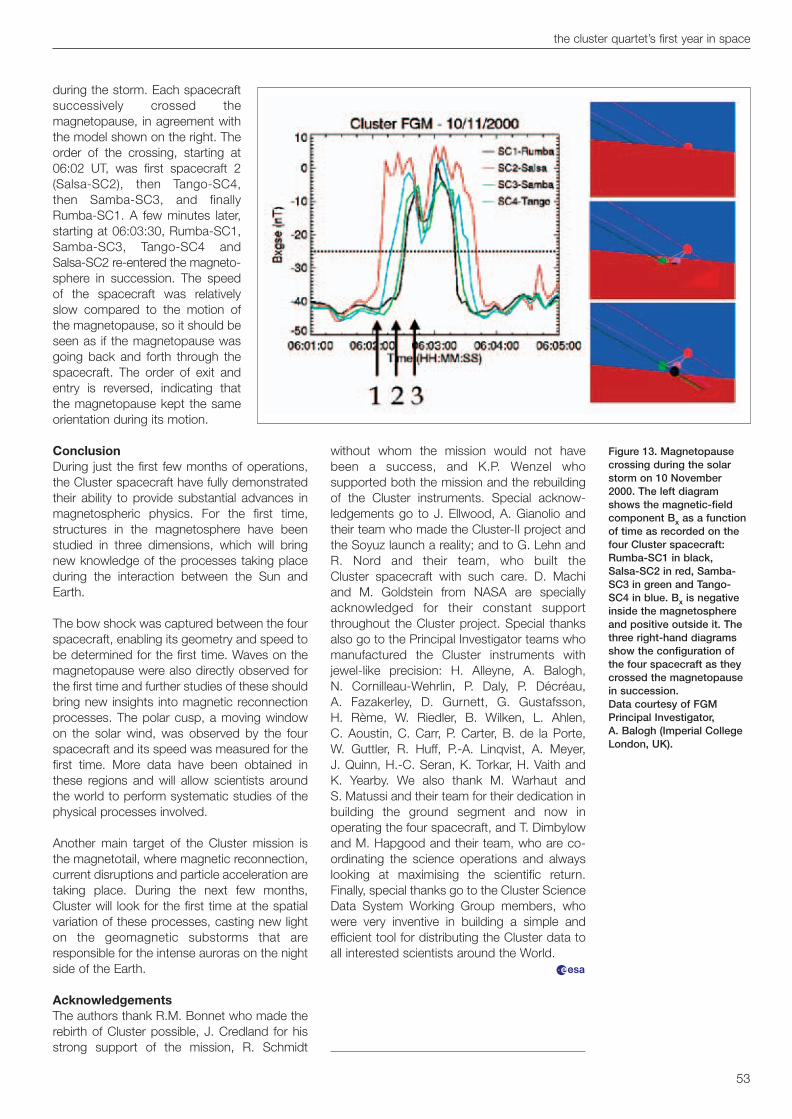
Figure 13. Magnetopausecrossing during the solarstorm on 10 November2000. The left diagramshows the magnetic-fieldcomponent Bx as a functionof time as recorded on thefour Cluster spacecraft:Rumba-SC1 in black, Salsa-SC2 in red, Samba-SC3 in green and Tango-SC4 in blue. Bx is negativeinside the magnetosphereand positive outside it. Thethree right-hand diagramsshow the configuration ofthe four spacecraft as theycrossed the magnetopausein succession.Data courtesy of FGMPrincipal Investigator, A. Balogh (Imperial CollegeLondon, UK).

without whom the mission would not havebeen a success, and K.P. Wenzel whosupported both the mission and the rebuildingof the Cluster instruments. Special acknow-ledgements go to J. Ellwood, A. Gianolio andtheir team who made the Cluster-II project andthe Soyuz launch a reality; and to G. Lehn andR. Nord and their team, who built the Cluster spacecraft with such care. D. Machiand M. Goldstein from NASA are speciallyacknowledged for their constant supportthroughout the Cluster project. Special thanksalso go to the Principal Investigator teams whomanufactured the Cluster instruments withjewel-like precision: H. Alleyne, A. Balogh, N. Cornilleau-Wehrlin, P. Daly, P. Décréau, A. Fazakerley, D. Gurnett, G. Gustafsson, H. Rème, W. Riedler, B. Wilken, L. Ahlen, C. Aoustin, C. Carr, P. Carter, B. de la Porte, W. Guttler, R. Huff, P.-A. Linqvist, A. Meyer, J. Quinn, H.-C. Seran, K. Torkar, H. Vaith andK. Yearby. We also thank M. Warhaut and S. Matussi and their team for their dedication inbuilding the ground segment and now inoperating the four spacecraft, and T. Dimbylowand M. Hapgood and their team, who are co-ordinating the science operations and alwayslooking at maximising the scientific return.Finally, special thanks go to the Cluster ScienceData System Working Group members, whowere very inventive in building a simple andefficient tool for distributing the Cluster data toall interested scientists around the World.

s

during the storm. Each spacecraftsuccessively crossed themagnetopause, in agreement withthe model shown on the right. Theorder of the crossing, starting at06:02 UT, was first spacecraft 2(Salsa-SC2), then Tango-SC4,then Samba-SC3, and finallyRumba-SC1. A few minutes later,starting at 06:03:30, Rumba-SC1,Samba-SC3, Tango-SC4 andSalsa-SC2 re-entered the magneto-sphere in succession. The speedof the spacecraft was relativelyslow compared to the motion ofthe magnetopause, so it should beseen as if the magnetopause wasgoing back and forth through thespacecraft. The order of exit andentry is reversed, indicating thatthe magnetopause kept the sameorientation during its motion.

ConclusionDuring just the first few months of operations,the Cluster spacecraft have fully demonstratedtheir ability to provide substantial advances inmagnetospheric physics. For the first time,structures in the magnetosphere have beenstudied in three dimensions, which will bringnew knowledge of the processes taking placeduring the interaction between the Sun andEarth.

The bow shock was captured between the fourspacecraft, enabling its geometry and speed tobe determined for the first time. Waves on themagnetopause were also directly observed forthe first time and further studies of these shouldbring new insights into magnetic reconnectionprocesses. The polar cusp, a moving windowon the solar wind, was observed by the fourspacecraft and its speed was measured for thefirst time. More data have been obtained inthese regions and will allow scientists aroundthe world to perform systematic studies of thephysical processes involved.

Another main target of the Cluster mission isthe magnetotail, where magnetic reconnection,current disruptions and particle acceleration aretaking place. During the next few months,Cluster will look for the first time at the spatialvariation of these processes, casting new lighton the geomagnetic substorms that areresponsible for the intense auroras on the nightside of the Earth.

AcknowledgementsThe authors thank R.M. Bonnet who made therebirth of Cluster possible, J. Credland for hisstrong support of the mission, R. Schmidt

the cluster quartet’s first year in space

53

ESCOUBET 24-08-2001 13:32 Page 13