esa eo based energy - connecting repositories4 market overview 4.1 general in contrary to other...
TRANSCRIPT

ESA ‐ RESGrow Expansion of the Market for EO Based Information Services in Renewable Energy Biomass Energy sector

Expansion of the Market for EO Based Information Services
in Renewable Energy
Biomass Energy Sector
Biomass study
submitted by
Deutsches Zentrum für Luft‐ und Raumfahrt e.V. (DLR)
Oberpfaffenhofen D‐82234 Wessling
Tel: ++49 8153 28 15 72 Fax: ++49 8153 28 14 58
ESA Contract No. 4000107680/13/I‐AM

Ref :4000107680/13/l‐AM Biomass study Page: 3
Preparation and signature list
Name and role Company
Prepared by Dr. Markus Tum
Dr. Kurt P. Günther
Dr. Marion Schroedter‐Homscheidt
DLR
Approved by Dr. Zoltan Bartalis
Ann Fitzpatrick
ESA
TechWorks Marine Ltd.
Date February 25th, 2014

Ref :4000107680/13/l‐AM Biomass study Page: 4
Table of contents
Biomass Energy Sector ............................................................................................................... 2
Biomass study ............................................................................................................................ 2
Table of contents ....................................................................................................................... 4
1 Summary ............................................................................................................................ 6
2 Study Concept .................................................................................................................... 8
3 Definitions .......................................................................................................................... 9
4 Market Overview ............................................................................................................. 11
4.1 General ...................................................................................................................... 11
4.2 Global ........................................................................................................................ 14
4.3 Europe ....................................................................................................................... 17
4.4 Stakeholder ............................................................................................................... 23
5 Technology Overview ....................................................................................................... 25
5.1 Need for Geoinfomation ........................................................................................... 32
5.1.1 Feasibility study and potential analysis ............................................................. 32
5.1.2 Site selection ...................................................................................................... 33
5.1.3 Permit stage ....................................................................................................... 35
5.1.4 Optimized design and engineering .................................................................... 35
5.1.5 Construction ....................................................................................................... 35
5.1.6 Operation, maintenance and monitoring .......................................................... 35
5.1.7 Decommissioning ............................................................................................... 36
6 Energy Crops .................................................................................................................... 37
7 Biomass Modelling ........................................................................................................... 39
7.1 Types of models and choice of the model and data ................................................. 39
7.2 Overview of institutions existing models .................................................................. 41
7.2.1 AGROSIM ............................................................................................................ 41
7.2.2 BETHY/DLR ......................................................................................................... 42
7.2.3 CERES and DSSAT ............................................................................................... 43
7.2.4 DNDC .................................................................................................................. 44
7.2.5 ECGM ................................................................................................................. 45

Ref :4000107680/13/l‐AM Biomass study Page: 5
7.2.6 EPIC .................................................................................................................... 46
7.2.7 FAO ..................................................................................................................... 47
7.2.8 G4M .................................................................................................................... 49
7.2.9 IBSAL .................................................................................................................. 49
7.2.10 MARS .................................................................................................................. 50
7.2.11 Further models approaches ............................................................................... 53
7.3 Empirical estimation of biomass potentials using remote sensing .......................... 54
8 Availability of EO and identified limitations .................................................................... 56
8.1 Biomass potentials .................................................................................................... 58
8.2 Land cover classification ........................................................................................... 59
8.2.1 Global Land Cover Characterisation (GLCC) ....................................................... 61
8.2.2 University of Maryland (UMD) 1km Global Land Cover .................................... 66
8.2.3 CORINE Land Cover Project................................................................................ 67
8.2.4 GLC 2000 ............................................................................................................ 69
8.2.5 MODIS LCC product ............................................................................................ 71
8.2.6 GLOBCOVER ....................................................................................................... 71
8.2.7 Future activities ................................................................................................. 73
8.3 Leaf Area Index .......................................................................................................... 73
8.3.1 LAI derived from the VEGETATION instrument ................................................. 73
8.3.2 GEOLAND LAI ..................................................................................................... 75
8.3.3 MODIS LAI .......................................................................................................... 76
8.4 Net Primary Productivity ........................................................................................... 78
8.5 Meteorological parameters ...................................................................................... 79
8.6 Photosynthetic active radiation ................................................................................ 79
9 References ....................................................................................................................... 80

Ref :4000107680/13/l‐AM Biomass study Page: 6
1 Summary
Biomass energy is of growing importance as it is widely recognised, both scientifically and politically, that the increase of atmospheric CO2 has led to an enhanced efficiency of the greenhouse effect and, as such, warrants concern for climate change. It is accepted (IPCC 2011 and just recently in the draft version of the IPCC 2013 report) that climate change is partly induced by humans notably by using fossil fuels. For reducing the use of oil or coal, biomass energy is receiving more and more attention as an additional energy source available regionally in large parts of the world. Effective management of renewable energy resources is critical for the European and the global energy supply system. The future contribution of bioenergy to the energy supply strongly depends on its availability, in other words the biomass potential. Biomass potentials are currently mainly assessed on a national to regional or on a global level, with the bulk biomass potential allocated to the whole country. With certain biomass fractions being of low energy density, transport distances and thus their spatial distribution are crucial economic and ecological factors. For other biomass fractions a super‐regional or global market is envisaged. Thus spatial information on biomass potentials is vital for the further expansion of bioenergy use. This study, which is an updated version of a study carried out in 2007 in frame of the ENVISOLAR project, analyses the potential use of Earth Observation data as input for biomass models in order to assessment and manage of the biomass energy resources especially biomass potentials of agricultural and forest areas with high spatial resolution (typical 1km x 1km). In addition to a sorrow review of recent developments in data availability and approaches in comparison to its 2007’ version, this study also includes a review on approaches to directly correlate remote sensing data with biomass estimations. An overview of existing biomass models is given covering models using remote sensing data as input as well as models using only meteorological and/or management data as input. It covers the full life cycle from the planning stage to plant management and operations (Figure 1). Several groups of stakeholders were identified. Limitations in Earth Observation data and downstream value adding chains were identified:
Land cover classification (LCC) databases typically do not distinguish between different energy crops or list only a small subset of them.
The moisture content of energy crops is not modelled.
Net primary productivity (NPP) is provided operationally by NASA and planned for by ESA, but not for different energy crops. Actual land cover classification is missing to extend NPP modelling.

Ref :4000107680/13/l‐AM Biomass study Page: 7
Therefore, spatial and temporal variability of the bioenergy resources is difficult to assess with the help of EO data in this case. Only experimental information restricted to a few crops based on a study level are available.
For forests, an initial database of biomass for a reference year is needed as NPP modelling provides only a yearly increment to be added to a reference year.
For forests, additionally information about the age of a tree population is needed to choose appropriate allocation rules for the estimation of trunk volume growth as a function of NPP.
However these limitations might be at least to some extend lowered with the possibilities the forthcoming Sentinel missions and the Biomass mission in special.
Figure 1: Decision support systems in different steps of the energy supply system

Ref :4000107680/13/l‐AM Biomass study Page: 8
2 Study Concept
The study focuses only on using biomass as an energy resource. The use of biomass as a resource for biodegradable materials and natural fibre reinforced plastics might be a future market. Nevertheless, the study concentrates on the energy market only as these other markets are not yet developed. Additionally, the already well‐established use of biomass for biogeneous lubricants, insulating and building materials is out of the focus of this study. Biomass consists of residues from forestry and agriculture, dedicated energy crops and the waste and residuals produced during the use of these substances. Excrements from human and animal origins, organic sludge, domestic and commercial waste of organic origin and paper is also part of the biomass used for energy supply in many cases. Concerning this study, waste is outside the scope of this study as such biomass is outside the monitoring capabilities of Earth Observation. Basis of this report is an extensive literature review based also on websites, scientific, and non‐scientific publications from other institutions. Focus is laid on the usage of Earth Observation to derive the technical potentials – further spatial information as e.g. population growth, per capita food consumption, efficiency of animal production systems, etc. are needed to address economic potentials. This is outside the scope of this study. After a definitions section of relevant terms used in the biomass / bioenergy discussion, section 3 gives a short overview on the global and the European market and its stakeholders. Section 4 provides a technology overview and reviews the need for geo‐information in different lifecycle steps. Section 5 gives an overview on energy crops used and section 6 reviews biomass modelling and resource assessment methods, before an analysis of availability of Earth Observation based information and a gap analysis is made in section 7.

Ref :4000107680/13/l‐AM Biomass study Page: 9
3 Definitions
This study follows the definitions as set up by the European Commission (2009) in its directive on biofuels. biomass biodegradable fraction of products, waste and residues from biological
origin from agriculture (including vegetal and animal substances), forestry and related industries including fisheries and aquaculture, as well as the biodegradable fraction of industrial and municipal waste.
biofuels liquid or gaseous fuel for transport produced from biomass. bioethanol ethanol produced from biomass. biodiesel methyl‐ester produced from vegetable or animal oil, of diesel quality,
to be used as biofuel. biogas a fuel gas produced from biomass and/or from the biodegradable
fraction of waste, that can be purified to natural gas quality, to be used as biofuel, or wood gas.
biobutanol butanol produced from biomass, to be used as biofuel biomethanol methanol produced from biomass, to be used as biofuel. biodimethyl‐ ether methanol produced from biomass, to be used as biofuel bio‐ETBE ethyl‐tertio‐butyl‐ether produced on the basis of bioethanol. bio‐MTBE methyl‐tertio‐butyl‐ether produced on the basis of bio‐methanol. Fischer‐Tropsch diesel a synthetic hydrocarbon or mixture of synthetic hydrocarbons
produced from biomass. hydrotreated vegetable oil vegetable oil thermo‐chemically treated with hydrogen. pure vegetable oil oil produced from oil plants through pressing, extraction or
comparable procedures, crude or refined but chemically unmodified,

Ref :4000107680/13/l‐AM Biomass study Page: 10
when compatible with the type of engines involved and the corresponding emission requirements.
Potential analysis generally distinguishes between: theoretical potential the theoretical maximum potential is limited by factors such as
the physical or biological barriers that cannot be altered given the current state of science. E.g. the theoretical potential yield of a crop is the yield that is limited by the efficiency of photosynthesis, other yield limiting factors can be compensated through technology.
technical potential the potential that is limited by the technology used and the
natural circumstances. E.g. the yield of a crop based a certain level of technology. The technical potential is the same as the theoretical potential if the technologies used that do not limit productivity.
economic potential the technical potential that can be produced at economically
profitable levels, depicted by a cost‐supply curve of secondary biomass energy.
implementation potential the potential that can be implemented within a certain timeframe, taking (institutional and social) constraints and incentives into account. The implementation potential can be smaller than the economic potential or larger – e.g. due to government aid.

Ref :4000107680/13/l‐AM Biomass study Page: 11
4 Market Overview
4.1 General
In contrary to other renewable energy sources, such as wind, solar and hydro, the nature of biomass is extremely variable and there are many possible routes for the conversion of biomass to bioenergy. Attention has to be paid not only to the energy conversion technology employed but also to the whole bioenergy supply chain starting from the energy crop resources as a function of space and time, logistics, stock keeping, the energy conversion module and the specific needs of the regional customer group. Failures in the past showed that profitability can only be achieved, if the whole chain is analysed and made consistent. Therefore, the choice of a certain energy conversion module is extremely dependent on the regional conditions, especially the availability of biomass resources which are needed to ensure secure energy supply. Up to now, mostly regional resources are used in bioenergy plants. Therefore, regional differences in price and quality levels are usual. Unified commodities as known from fossil fuels exist only for pellets, old timber and biofuels (e.g. biodiesel or palm oil). Both, old timber and pellets are relatively easy to transport and to store. Therefore, a supra‐regional market exists. Examples are Austrian wood chips sold in Germany or old timber collected on a European level. Until the mid of the 20th century, trading cereals was a regional or national market. Transport of corn was too expensive in contrary e.g. to the trade of spices which have been transported between continents for centuries. Only due to a strong decrease in transportation costs since 1950 e.g. for the line USA‐Europe an international and nowadays global market for cereals was created. It has to be taken into account that energy crops could face a similar development in the next decades. In case the market turns from a regional to an international or even global market, spatial geo‐information on energy crop yields will be needed. First signs are reports on existing or planned transports of wood chips from Austria to Germany or other European countries. For other biomass resources without supra‐regional markets yet, the biomass supply chain has to be optimised for each bioenergy plant individually. A supply chain relies on:
minimized transport costs
optimized storage to cope with seasonal availability and necessary drying processes
purchase in low price seasons as much as storage facilities allow
increased supply security through storage facilities or highly reliable suppliers

Ref :4000107680/13/l‐AM Biomass study Page: 12
long‐term supply contracts
reliable estimates of future biomass availability and competing demand
quality control of resources and probably a mixture of charges to ensure a continuous quality level
In future according to IEA (2011), a global market for biomass products can be envisaged taking advantage of different climates and types of vegetation around the world. There is an increasing interest in ethanol as an alternative transport fuel but currently few countries plant significant amounts of plants such as sugar cane for this purpose. Brazil, one of the forerunners in this field, is a major producer and exporter of this product with a volume of about 21100 billion litres and some 25% of the world's ethanol production market. The Netherlands forecast a significant biomass market in Europe in their energy transition strategy with major supplies expected to come from Scandinavian forestry. The boundaries that seasonal cycles put on the maximum amount of energy derived from biomass can thus be extended, but will ultimately run into competition from other land use interests and possibly competing uses of biomass itself. If current growth forecasts of biomass usage become reality seasonal cycles will surface more prominently on the policy agenda. A variety of technologies is available to generate heat, liquid fuels and/or electrical power from energy crops, agricultural and forest residues, organic residues and organic waste. Concerning energy crops and residues, bioenergy can be seen as a manifestation of the solar energy (Fehler! Verweisquelle konnte nicht gefunden werden.) as biomass growth is dependent on solar energy provided by the sun.

Ref :4000107680/13/l‐AM Biomass study Page: 13
Figure 2: Overview on renewable energies (BMU, 2011a)

Ref :4000107680/13/l‐AM Biomass study Page: 14
4.2 Global
More than a quarter of the world’s population has no access to electricity, and two‐fifths still rely mainly on traditional biomass for their basic energy needs (IEA, 2011). This explains that global primary energy consumption shows a large share of more than 10% for biomass while the renewable energy sources overall contribute to 19% (Figure 3).
Figure 3: Global primary energy consumption (REN21, 2013) Following the World Energy Outlook (IEA, 2011), poor people in developing countries rely heavily on traditional biomass – wood, agricultural residues and dung – for their basic energy needs e.g. for cooking and heating. Over half of all people relying heavily on biomass live in India and China, but the proportion of the population depending on biomass is heaviest in sub‐Saharan Africa. The share of the world’s population relying on biomass for cooking and heating is projected to decline in most developing regions, but the total number of people will rise. Most likely this increase will occur in e.g. South Asia and sub‐Saharan Africa. The World Energy Outlook estimates, that more than 50% of the increase in world primary energy demands between 2000 and 2035 will come from developing countries, especially in Asia. The surge in demand in the developing regions results from their rapid economic and population growth. Industrialisation and urbanisation will also boost demand. The replacement of traditional biomass by commercially traded energy will increase recorded demand. For renewables, it is expected that wind power and biomass will grow most rapidly, especially in OECD countries. Non‐hydro renewables grow faster than any other source, at an annual rate of 4% world‐wide, and the total output from renewables increases almost
Ref :4000107680/13/l‐AM Biomass study Page: 15
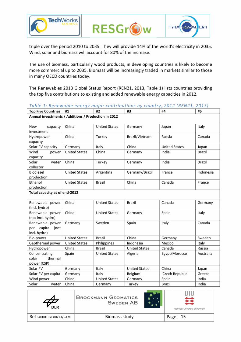
triple over the period 2010 to 2035. They will provide 14% of the world’s electricity in 2035. Wind, solar and biomass will account for 80% of the increase. The use of biomass, particularly wood products, in developing countries is likely to become more commercial up to 2035. Biomass will be increasingly traded in markets similar to those in many OECD countries today. The Renewables 2013 Global Status Report (REN21, 2013, Table 1) lists countries providing the top five contributions to existing and added renewable energy capacities in 2012. Table 1: Renewable energy major contributions by country, 2012 (REN21, 2013) Top Five Countries #1 #2 #3 #4 #5
Annual investments / Additions / Production in 2012
New capacity investment
China United States Germany Japan Italy
Hydropower capacity
China Turkey Brazil/Vietnam Russia Canada
Solar PV capacity Germany Italy China United States Japan
Wind power capacity
United States China Germany India Brazil
Solar water collector
China Turkey Germany India Brazil
Biodiesel production
United States Argentina Germany/Brazil France Indonesia
Ethanol production
United States Brazil China Canada France
Total capacity as of end‐2012
Renewable power (incl. hydro)
China United States Brazil Canada Germany
Renewable power (not incl. hydro)
China United States Germany Spain Italy
Renewable power per capita (not incl. hydro)
Germany Sweden Spain Italy Canada
Bio‐power United States Brazil China Germany Sweden
Geothermal power United States Philippines Indonesia Mexico Italy
Hydropower China Brazil United States Canada Russia
Concentrating solar thermal power (CSP)
Spain United States Algeria Egypt/Morocco Australia
Solar PV Germany Italy United States China Japan
Solar PV per capita Germany Italy Belgium Czech Republic Greece
Wind power China United States Germany Spain India
Solar water China Germany Turkey Brazil India

Ref :4000107680/13/l‐AM Biomass study Page: 16
collector (heating)
Solar water collector (heating) per capita
Cyprus Israel Austria Barbados Greece
Geothermal heat capacity
United States China Sweden Germany Japan
Table 2 adds an overview on global existing capacities for power generation, heating, transport fuels and rural off‐grid energy from renewable energies including biomass use (REN21, 2013). Biomass power generation and heat supply continued to increase at both large and small scales, with an estimated 9 GW power capacity added in 2012, bringing existing biomass power capacity to about 83 GW. Annual increases of up to 100 % in biomass power production were registered in the past years in several OECD countries. There is an increasing proliferation of small and bigger projects in developing countries, such as Pakistan’s “Alternative Energy Developing Board”, which will result in the next years in five or more biomass power plants with altogether 57 GW. Bagasse power plants are under development by the sugar industry in several countries, such as the Philippines, Pakistan and Brazil. Geothermal power saw continued growth as well. Ethanol production slightly decreased to 83.1 billion litres in 2012, down from 84.0 billion litres in 2011 ‐ a 1.1 % decrease, with most of this in the United States and Brazil. Overall, the United States accounted for 61% (63% in 2011) of global ethanol production and Brazil for 26% (25% in 2011). Fuel ethanol consumption in Brazil was fairly stable, whereas it dropped by 4% in the U.S. Brazil’s vehicle market is constantly shifting towards “flex‐fuel” vehicles, which already attained a 70 % share of the (non‐diesel) vehicle market in 2005 and gained of more importance until now. In total bioethanol far outpaced ethanol. Global production of biodiesel reached 22.5 billion litres, whereas ethanol reached 83.1 billion litres. The ethanol fuel market is already dominated by trade flows as e.g. from Brazil to the USA and in future exports from Brazil and USA to the EU, Asia and the USA are expected. In this sector bioenergy has become a tradable good already and world‐wide markets exist. It is expected that the ethanol fuel market will get an equal importance as the nowadays sugar market. For other bioenergy types this development is foreseen for the upcoming years.

Ref :4000107680/13/l‐AM Biomass study Page: 17
Table 2: Renewable Energy added and existing capacities, 2012 (REN21, 2013)
4.3 Europe
Biomass contributes to 13% of total EU primary energy production (Figure 4), predominantly in heat and to a lesser extent, in combined heat and power (CHP) applications. A rather new trend is the cooling of buildings, technical facilities (e.g. IT infrastructures) or industrial buildings based on bioenergy. By 2020, renewables are forecasted to cover as much as 20.7% of the total EU energy supply (BMU, 2011b). The heat/cold sector will continue to be dominated by biomass, with a share

Ref :4000107680/13/l‐AM Biomass study Page: 18
of 77.6 %. According to the predictions by the EU Member States, biodiesel will make the largest renewable contribution in the transport sector with 64.8 %.
Figure 4: Production of primary energy, EU‐27, 2009 (BMU, 2011b)
Nowadays, there are large differences between the European countries. While Norway, Latvia Sweden, Austria and Finland reach a biomass share of primary energy consumption above 20% (Figure 5 and Table 3), other countries as Belgium, Irleand, The Netherlands and the United Kingdom achieve only a few percent (below 5 %) contribution (EU, 2012).

Ref :4000107680/13/l‐AM Biomass study Page: 19
Figure 5: Structure of renewable energy sources as a share of primary energy consumption (EU, 2012)

Ref :4000107680/13/l‐AM Biomass study Page: 20
Table 3: Use of renewable energy sources and installed capacity in the EU, 2009/2010 (BMU, 2011b)

Ref :4000107680/13/l‐AM Biomass study Page: 21
On the policy level, two European directives on renewable energy sources and biofuels need to be mentioned: The directive 2009/28/EC of the European parliament and of the council of 23 April 2009 on the promotion of the use of energy from renewable sources and amending and subsequently repealing Directives 2001/77/EC and 2003/30/EC defines a global indicative a target of 20 % for the overall share of energy from renewable sources and a target of 10 % for energy from renewable sources in transport by 2020. The directive 2003/30/EC of the European parliament and of the council of 8 May 2003 on the promotion of the use of biofuels or other renewable fuels for transport which now is embedded in the directive 2009/28/EC emphasizes:
There is a wide range of biomass that could be used to produce biofuels, deriving from agricultural and forestry products, as well as from residues and waste from forestry and the forestry and agrifoodstuffs industry.
The transport sector accounts for more than 30 % of final energy consumption in the Community
The Commission White Paper ‘European transport policy for 2010: time to decide’ expects CO2 emissions from transport to rise by 50 % between 1990 and 2010, to around 1 113 million tonnes, the main responsibility resting with road transport, which accounts for 84 % of transport‐related CO2 emissions. From an ecological point of view, the White Paper therefore calls for dependence on oil (currently 98 %) in the transport sector to be reduced by using alternative fuels such as biofuels.
As a result of technological advances, most vehicles currently in circulation in the European Union are capable of using a low biofuel blend without any problem. The most recent technological developments make it possible to use higher percentages of biofuel in the blend. Some countries are already using biofuel blends of 10 % and higher.
Pure vegetable oil from oil plants produced through pressing, extraction or comparable procedures, crude or refined but chemically unmodified, can also be used as biofuel in specific cases where its use is compatible with the type of engines involved and the corresponding emission requirements.
Bioethanol and biodiesel, when used for vehicles in pure form or as a blend, should comply with the quality standards laid down to ensure optimum engine performance. It is noted that in the case of biodiesel for diesel engines, where the processing option is esterification, the standard prEN 14214 of the

Ref :4000107680/13/l‐AM Biomass study Page: 22
European Committee for Standardisation (CEN) on fatty acid methyl esters (FAME) could be applied.
Promoting the use of biofuels in keeping with sustainable farming and forestry practices laid down in the rules governing the common agricultural policy could create new opportunities for sustainable rural development in a more market‐orientated common agriculture policy geared more to the European market and to respect for flourishing country life and multifunctional agriculture, and could open a new market for innovative agricultural products with regard to present and future Member States.
The Commission Green Paper ‘Towards a European strategy for the security of energy supply’ sets the objective of 20 % substitution of conventional fuels by alternative fuels in the road transport sector by the year 2020.
In its resolution of 18 June 1998, the European Parliament called for an increase in the market share of biofuels to 2 % over five years through a package of measures, including tax exemption, financial assistance for the processing industry and the establishment of a compulsory rate of biofuels for oil companies.
National indicative targets: o A reference value for these targets shall be 2 %, calculated on the basis of
energy content, of all petrol and diesel for transport purposes placed on their markets by 31 December 2005. A reference value for these targets shall be 5,75 %, calculated on the basis of energy content, of all petrol and diesel for transport purposes placed on their markets by 31 December 2010.
Biofuels may be made available in any of the following forms: o as pure biofuels or at high concentration in mineral oil derivatives, in
accordance with specific quality standards for transport applications; o as biofuels blended in mineral oil derivatives, in accordance with the
appropriate European norms describing the technical specifications for transport fuels;
o as liquids derived from biofuels, such as ETBE (ethyl‐tertiobutyl‐ether), where the percentage of biofuel is as specified in Article 2(2).
Member States shall report to the Commission, before 1 July each year, on: the national resources allocated to the production of biomass for energy uses other than transport, and the total sales of transport fuel and the share of biofuels, pure or blended, and other renewable fuels placed on the market for the preceding year. Where appropriate, Member States shall report on any exceptional conditions in the supply of crude oil or oil products that have affected the marketing of biofuels and other renewable fuels.
Ref :4000107680/13/l‐AM Biomass study Page: 23
4.4 Stakeholder
In the following chapter stakeholders relevant for bioenergy power plants as well as their functions are summarized. Suppliers of combustibles: Function:
treatment
storage to cope with temporal shift between production and usage
storage to cope with regional and seasonal variability in supply and demand
guarantee of secure supply structures
transport and logistics
organising distribution channels for overproducts in the agricultural sector
acting as brokers between producers and customers Typical stakeholders
individual farmers and farmer associations for arable crops
forest enterprises for thinning material and forest residuals
regional nature conservation authorities for material from landscape conservation
local authorities and road operation centres for logging
wood industries and dealers for timber and forest residuals
recycling companies for timber Operator/Owner of a bioenergy power plant Function:
financing
building
regular operations
maintenance
secure commodity supply
selling bioenergy Typically this role is fulfilled by a dedicated operating company or a electrical utility. Customers needing heat and electricity
private households
building contractors
cooperatives
public buildings
commercial and industrial companies
trading companies
users of thermal heat and processing water
Ref :4000107680/13/l‐AM Biomass study Page: 24
sometimes process heat
electric utilities
electricity grid operators Financing companies and funding authorities Function: investment, funding Authorising agencies Function: permit Planning companies Function:
project development
preliminary, blueprint and approval planning
implementation planning
tendering and awarding of contracts
coordination of suppliers Power plant engineers Function: Building of the power plant Further stakeholders: International organisations like Food and Agriculture Organisation (FAO) of the United Nations, the International Energy Agency (IEA) and the World Bank. Participants of the International Energy Agency technology agreements ‚Short rotation crops’, ‚Biomass production for energy from sustainable forestry’, ‚Biomass combustion and co‐firing’, ‚Greenhouse gas balances of biomass and bioenergy systems’, ‚Liquid biofuels from biomass’, ‚Sustainable international bioenergy trade’, and ‚Bioenergy systems analysis’. Industry associations like the European Biodiesel Board (EBB), the European Bioethanol Fuel Association (eBIO) or the national U.S. Renewable Fuels Association (RFA), and the Canada Renewable Fuels Association. Public bodies like European Commission, its Joint Research Centre (JRC), national ministries and public authorities in the fields of energy production and environmental protection.

Ref :4000107680/13/l‐AM Biomass study Page: 25
5 Technology Overview
Bioenergy can be roughly divided into three classes:
Solid biomass as e.g. wood chips and pellets
Liquid biofuels as e.g. biodiesel, bioethanol or second generation biofuels
Biogas as e.g. from municipal or agricultural waste
In this chapter an overview on different energy conversion techniques from biomass to bioenergy is given (Figure 6). This chapter follows widely a description taken from (BMU, 2011a and IPCC, 2011)
Figure 6: Schematic view of commercial bioenergy routes (IPCC, 2011a). Notes: 1. Parts of each feedstock, for example, crop residues, could also be used in other routes. 2. Each route also gives co‐products. 3. Biomass upgrading includes any one of the densification processes (pelletization, pyrolysis, etc.). 4. Anaerobic digestion processes release methane and CO2 and removal of CO2 provides essentially methane, the main component of natural gas; the upgraded gas is called biomethane
Biomass has so far mainly been cultivated for the production of food and fodder. However, it is increasingly used for energy or substance (renewable resources for the chemical, pharmaceutical, or construction industries). Today, mostly organic residuals and waste materials are used for electricity and heat generation. To an increasing degree, energy crops are also being cultivated for the production of biofuels.

Ref :4000107680/13/l‐AM Biomass study Page: 26
The oldest and simplest way of using energy is to burn the biomass. Different types of burning were developed for various plant sizes to assure complete combustion and low emissions, considering the ash content, the fuel composition, and the shape and size of the fuel particles. They essentially differ in the type of fuel processing and the fuel feed method. Present‐day use of biogenous solid fuels is mostly in very small systems (less than 15 kW) or in small‐scale systems. Automated fuel feed, together with a suitable combustion control system, have increased the ease of operation. Wood‐pellet furnaces are currently enjoying a wave of popularity. Wood pellets are small compressed beads of untreated wood, usually from sawdust and plane shavings. They can be delivered like heating oil by tank trucks, or sold in sacks. Pellets can be fired in chimney stoves just like in large‐scale, fully‐automated and low emission central heating systems. The pellets are automatically transported from a storage container to the furnace chamber by means of screw conveyors or suction feeders. The space needed for storing this type of fuel is hardly larger than for an oil‐fired central heating system. Generating heat is not limited to small‐scale systems only. Firing wood can also be used for district heating networks. In Austria, a country which has been systematically supporting the use of biomass for many years now, there are already several hundred district heating plants running on biomass. It is worthwhile to invest in greater technical optimisation of these larger incineration facilities. Both the efficiencies and the emissions of modern furnaces have been improved. For example, the efficiency can be increased considerably by condensing the flue gases, since the transformation energy when the water vapour condenses into liquid can be used, and by predrying the biomass. Electricity from biomass The interest in producing electricity from biomass has increased considerably and different principles for converting solid biomass to electricity are possible (Figure 7). The preferred fuel in the newly constructed power stations is almost exclusively cost‐effective old timber. Economic operation of the plants is not possible with the more expensive untreated wood. The days of being able to charge a disposal fee for accepting contaminated wood are long gone because of the considerably increased demand for this wood. Biomass for electricity generation is particularly important to the power industry because it is always available and can be converted to electricity according to the demand. In modern wood‐fuelled power plants, the biomass is burned and steam is usually generated with the heat. This steam then drives a turbine or a motor. It is particularly efficient to use the waste heat for heating buildings or for drying processes as combined heat and power generation, instead of simply dissipating it into the surrounding environment.

Ref :4000107680/13/l‐AM Biomass study Page: 27
The Organic Rankine Cycle (ORC) is particularly suited for heat sources at a low temperature level. In this process the combustion heat – or heat from any other source, e.g. geothermal – is not used to generate steam for a steam turbine. Instead, an organic solvent, e.g. toluene, pentane, or ammonia, is evaporated and used to drive a turbine. Of the plants under construction in Germany at the end of 2010, already 52 % employ the innovative ORC method which is particularly suitable for central biomass cogeneration plants. A promising alternative to burning is the gasification of biomass. In this process, the biomass is decomposed at high temperatures and transformed into a gas, which is then cooled off, cleaned, and then fired in a motor cogeneration plant or a turbine. The future use of biomass in fuel cells, which provide high yields of electricity even from small‐power units, is possible with gasified wood. The principle of wood gasification is not new. It was used e.g. after the war for powering lorries due to the lack of more motor‐gentle fuels. The trick is to produce a high‐quality and tar‐free gas, whose continuous use is tolerated by motors, from varying fuel qualities. Biogas can also be used to generate electricity, preferably in cogeneration units. Biogas is liberated when organic material is decomposed by special methane bacteria. This process is called fermentation. Two major prerequisites must be met to obtain an energy‐rich gas: anaerobic (oxygen‐free) conditions must prevail, and the temperatures in the biogas reactor must be suitable for the desired bacteria. Most biogas systems operate at temperatures between 30 and 37 °C. The bacteria decompose the organic matter in several stages. The final products of this decomposition chain are the gases methane (CH4) and carbon dioxide (CO2). One hundred cubic meters of biogas develop from between a half and one ton of bio‐waste, corresponding to the daily excrement from 90 cows or 12,000 chickens. With a calorific value of about 6 kWh, one cubic meter of biogas is equivalent to 0.6 litres of heating oil or 0.6 m3 of natural gas. Biogas is suitable as a fuel for combustion engines. In Germany, reactor‐formed biogas is almost exclusively used in cogeneration units. The biogas can also be cleaned and fed into a natural gas grid or used as a rather efficient fuel in the transport sector.

Ref :4000107680/13/l‐AM Biomass study Page: 28
Figure 7: General principle of generating electricity from biomass (BMU, 2011a)
Biofuels All in all, transportation is the second largest energy consumer after households, closely followed by industry. Biofuels offer a good opportunity to partially substitute petroleum as an energy carrier in the transport sector. There is not just the one biofuel, but rather a whole range of liquid and gaseous bio‐energy carriers which can be used in the transportation sector. Possible pathways to produce fuels from renewable energy carriers are presented in Figure 8. Best known among the liquid biofuels are the vegetable oils from rapeseed and sunflower seeds, and the processed form of rapeseed oil called biodiesel (methyl ester from rapeseed oil). Ethanol from sugar beets, grain, potatoes, etc., and fuels made from lignocellulosis material like the so‐called biomass‐to‐liquid (BTL) fuels are major liquid biofuels derived through fermentation. Several kinds of gaseous biofuels are being discussed, like e.g. biogas, sewage gas, and landfill gas, as well as bio‐hydrogen and wood gas, which are more or less suitable for use in transportation. The feedstock is equally diverse, as they originate from agriculture, forestry, and fishery, from residual and waste materials, or as products from thermo‐chemical processes.

Ref :4000107680/13/l‐AM Biomass study Page: 29
Figure 8: Some possible pathways to produce fuels from renewable energy carriers (BMU, 2011a)
Right from the start, the inventor of the diesel engine foresaw the use of biofuel for his engine. “The use of vegetable oil as a fuel might be insignificant today. Yet, over time, these fuels could become as important as paraffin and the coal‐tar products of today”, noted Rudolf Diesel 1912 in his patent. Rape‐seed biodiesel (RME), also known as FAME (fatty acid methyl ester), is the most widespread biofuel in Germany – with a strongly increasing trend. A third of the biodiesel was admixed with conventional diesel; the rest was used in its pure form to fuel lorries and passenger cars. Unresolved problems are the coldstart properties of the cold‐sensitive oil, compliance with the more stringent EURO‐4 emission control requirements, and the energy balance if fertilisation and yield effort ist taken into account, so that its use will remain limited to niche applications. In Germany, e.g. tax reductions will decrease in the upcoming years, while the research effort to second generation biofuels (see below) is increased currently overall in Europe. Besides rapeseed and other oilseeds like soy or sunflower, imported palm oil is also being considered, and to a certain extent already employed, as a raw material for the production of biodiesel. However, new oil palm plantations must be cultivated in order to achieve an appreciable market share – in no way at the expense of tropical rainforests. The alcohols ethanol and methanol are very suitable for use as fuels in transportation, proven by years of experience. Even Nikolaus August Otto, the inventor of the spark‐ignition engine, used ethanol as the fuel when developing his engine and Henry Ford also designed his famous Model T to run on ethanol. Pure ethanol can only run special motors, like those found in Brazil’s vehicle fleet in the eighties, or those used in the so‐called “Flexible Fuel Vehicles”. A small fleet of these is operating in Sweden and in the United States. A more simple method is to add bioethanol to petrol, by which means bio‐ethanol could be introduced into the market with little effort. Up to 5 % by volume are allowed by the German standards without causing any problems to today’s vehicles. Pure bio‐ethanol can

Ref :4000107680/13/l‐AM Biomass study Page: 30
be used or – with an additional positive environmental effect – its derivative ETBE (ethyl tertiary butyl ether). ETBE could replace the octane enhancer MTBE (methyl tertiary butyl ether), which is added to petrol, and thereby reduce the emission of air pollutants. However, it has not yet been clarified whether ETBE, compared to MTBE, is less hazardous to the ground water. In any case, MTBE has already been banned in both California and Denmark for this reason. The almost legendary Brazilian bio‐ethanol vehicle fleet is however declining strongly. Besides biodiesel and bio‐ethanol, both of which are already commercialised, other processes are still being developed. The development goals for these “second generation biofuels” are to expand the range of possible application, to develop efficient processes, and to lower the production costs. Some of the processes rely on the gasification of biomass. If wood, straw, or other biomass sources are converted into a liquid fuel by means of a so‐called Fischer‐Tropsch process after gasification, then the energy of the entire plant can be utilised – which is not the case for biodiesel production from rapeseed. From the environmental and natural conservation point of view, these innovative technologies are more promising than biodiesel and bioethanol. Experts call this fuel BTL, for “biomass‐to‐liquid”; marketing experts named it “SunDiesel”. These fuels possess excellent combustion properties, which is why the automotive industry is waiting for these fuels to be produced. It would allow using the existing infrastructure of vehicles and petrol station infrastructure. None of the many manufacturing techniques have reached technical maturity yet. Gasified biomass does not necessarily need to be converted into a liquid fuel. The gas can also be conditioned and fed into the natural gas grid – known as biomethane – or the hydrogen can be separated from it and used in fuel cell vehicles or special hydrogen combustion engines. Biogas which is not produced through the gasification of biomass, but rather through the bacterial fermentation of manure, maize, or other energy plants can be employed in motor vehicles just like natural gas or bio‐methane. For this purpose, it must then be conditioned until it has the same quality as natural gas and is chemically identical with bio‐methane from biomass gasification. Although this option is technically possible, it is prohibitively expensive so far. However, the interest in biogas (biomethane) is clearly increasing with the growing popularity of natural‐gas vehicles in Germany. Biogas has already been employed as a fuel for some years in Switzerland, Sweden, and other countries. A feature of biogas, like BTL, is that the energy content of the entire plant is utilised through the fermentation of energy plants. The processes in bioethanol production are also being optimised. A technique is being developed which allows the utilisation of cellulose from wood and straw to produce fuel. It uses, e.g., enzymes to break down the cellulose molecule. The cellulose treated in this way can then be fermented. Overall, a variety of different technologies is used to derive heat and power from energy crops, agricultural and forest residues, organic residues and organic waste (Figure 9).

Ref :4000107680/13/l‐AM Biomass study Page: 31
Figure 9: Examples of stages of development of bioenergy: thermochemical (orange), biochemical (blue), and chemical routes (red) for heat, power, and liquid and gaseous fuels from solid lignocellulosic and wet waste biomass streams, sugars from sugarcane or starch crops, and vegetable oils. (IPCC, 2011)

Ref :4000107680/13/l‐AM Biomass study Page: 32
5.1 Need for Geoinfomation
In the next sections the life cycle of a bioenergy system is analysed for its needs for geoinformation. A large variety of environmental information needs to be considered (Figure 10).
Figure 10: Various environmental and social issues have to be addressed in bioenergy projects (IEA, 2007)
5.1.1 Feasibility study and potential analysis This first step is typically dedicated to the analysis of larger regions investigating where and how much biomass is expected. This analysis requires large scale information on the bioenergy resources. As we focus in this study on bioenergy derived from energy crops and forests, mainly vegetation monitoring on a large scale (region, country, continent) is required. Chapter 5 focuses more specifically on resource assessment methods for biomass using Earth Observation data. Typical is that first information on a region is needed if a stakeholder company starts its activities in a certain region. This includes information on local and regional bioenergy resources including their inter‐annual variability.

Ref :4000107680/13/l‐AM Biomass study Page: 33
It should be noted, that nowadays biomass is traded only partly which means that also taxes are applied only partly. This leads to gaps in the accurate statistical assessment of the actual use and potential of biomass. Also, in nowadays statistics the yield of crops as e.g. seeds or grain is monitored as known from traditional agriculture monitoring, but for the upcoming 2nd generation of bioenergy the full crop can be used. Partly, this can be calculated from the knowledge about crop yields as seeds using statistical information on the grain/stem relationship. Such relationships are relatively constant for each crop type, only the yield is variable as a function of environmental conditions. But besides these ‚conventional’ energy crops used in 1st generation bioenergy products, for the 2nd generation usage other energy crops and vegetation materials are used. Statistics about these resources are restricted as there has been no interest in these up to now. Resource management should include information about variability due to weather conditions with their inter‐annual variability. As global change is expected to cause more weather extremes, the focus on yield variability due to weather conditions is of increasing importance. This calls for dynamic vegetation modelling on the basis of yearly updated vegetation and land use information. Geoinformation is also needed to address issues like spatial clustering and trends of bioenergy resources. This allows analysing export potentials and European material flows. For the assessment of competitive use of land, information about local food demand and population growth is useful. In some areas of the world a specific wood demand for the traditional biomass use for heating and cooking has to be taken into account.
5.1.2 Site selection After a first potential analysis on a typically regional or country wide scale a more detailed analysis is undertaken to identify optimum sites for bioenergy power plants. This requires more detailed information on bioenergy resources in a better spatial and temporal resolution on a regional level. Chapter 5 focuses on resource assessment methods for biomass from energy crops and forests also on the regional scale. Typically, the choice of bioenergy technologies is dominated by the local availability of biomass resources of a certain type e.g. wood chips, waste, perennial crop etc. This is due to rather large costs for transport and storage of biomass. Often, the distance between farmland and the first storage facility (at the plant or an intermediate supplier) is only 5‐10 km. A wrong decision on combustibles/biomass types can result in higher costs than
Ref :4000107680/13/l‐AM Biomass study Page: 34
expected and necessary. Often, assumptions on available amounts of different biomass types turn out to be wrong. Therefore, a first step in project development is setting up a concept for biomass usage related to the local and regional conditions and taking into account knowledge on the supra‐regional resource market. This concept needs to address:
a typical mean transport distance relevant for the bioenergy plant
the seasonal cycle of regional biomass as a basis for a concept of long term centralised or de‐centralised storage
typical water content and calorific value of available biomass
bulk density to assess the necessary transport and storage volumes
delivery format in bales, pellets, wood chips, or bulk commodities
necessary treatment steps of biogenic combustibles used The long‐term storage is typically placed at the suppliers premises, but a short‐term storage is also needed next to the bioenergy plant. Its storage dimension is dependent on the harvesting and processing steps of the different combustibles used as e.g. wood chips have a storage need 10 times higher than mineral oil, while straw bales have a factor of 17 and wood pellets a factor of 3 (FNR, 2007). Additionally, the heating value of biomass can be compared against fossil combustibles: Related to mass the heating value of solid biomass is lower by a factor of 2 to 3, while the volume related heating value is lower by a factor of 10 (FNR, 2007). Again, this draws the attention on optimised transport and storage capacities adapted to regional and local resources. Also, short‐term storage allows coping with seasonal variability of biomass prices and should be dimensioned suitable for this. De‐central small systems (100 kW) for single buildings and medium plants (up to 10 MW) for housing or commercial areas are typical. These systems have an urgent need for local biomass supply to reduce transportation costs. Larger plants (up to 100 MW) are only used in cogeneration plants with fossil fuel usage for peak load situations and co‐firing of biomass (FNR, 2007). Bioenergy plants using mainly forest residues will also be preferably placed close to the local resources due to large transportation costs. In contrary, wood chips and pellets are more suitable for transportation, but need further processing steps to increase energy yield per cubic metre transport volume. Typically, storage of biomass generates extra costs and the optimum between constant biomass availability through storage and storage costs has to be looked for. For crops

Ref :4000107680/13/l‐AM Biomass study Page: 35
without longer drying periods, the time of harvest influences the market and thus annual cost optimization. Therefore, yield predictions concerning biomass amount, but also harvest time are useful. Cumulative NPP information on a weekly and monthly basis is of help for such an approach. In agricultural areas, a large slope angle is also a criterion for the definition of exclusion areas.
5.1.3 Permit stage Geo data needs in the permit stage are mostly related with land register databases and standard geoinformation as used in the approval process for any industrial building. Additional data bases are e.g. nature conservation area listings. Typically, such data is provided by local or regional authorities. Land use data might be used on the basis of satellite remote sensing depending on local conditions. Geo data might be also needed to address environmental and societal issues as local water supply, food production, nature conservation, health protection and air pollution etc.
5.1.4 Optimized design and engineering An optimized design follows the principles already mentioned in chapter ‚site selection’. Again, the seasonal variability in combustibles has to be taken into account together with an annual variability according to environmental conditions. And as mentioned before, logistics are relevant depending on harvesting and processing steps due to the low energy density of biomass. As an example, wood pellets and chaffed straw has a relation of 1:8 in the need of storage volume and requires different design strategies.
5.1.5 Construction Geo data on existing infrastructure might be of interest.
5.1.6 Operation, maintenance and monitoring Annual yield forecasts of biomass resources based on continuous monitoring of the vegetation state will help to deal with inter‐annual variability. The moisture content of biomass is a function of local weather conditions and can be included in operation strategies. Higher moisture content reduces the heating value in

Ref :4000107680/13/l‐AM Biomass study Page: 36
combustibles as some of the heat liberated during combustion is used up in evaporating the water. Higher moisture content also increases the water content in oil pressed e.g. from rape seed. Both effects create the need of changing technical process parameters (e.g. air/fuel ratio in combustion) for heating or oil production each year to cope with changing moisture content. Also, emissions of CO and NOx are a function of combustion parameters and therefore the moisture content (FNR, 2007). Moisture content in biomass causes also further problems in storage facilities: losses due to bio‐degradation, spontaneous combustion due to fermentation processes, high mould concentrations which affect human health, and odour (FNR, 2007). Therefore, storage duration has to be minimized. All these effects doesn’t occur if the moisture content is below 15 % which needs to be gained through dedicated drying processes and storage principles e.g. with good air circulation and coarse material structure which allows air to flow inside the storage. Drying effort depends on the water content at the harvesting time and is dependent on environmental conditions. These conditions might be monitored on spatial scales using meteorological and EO information. Technical drying procedures are typically too expensive. Therefore, passive drying is performed while wood is stored in the forest for over a year. This reduces the water content from approx. 45‐55 % down to below 30 %. In case of unsustainable agricultural management e.g. in tropical areas, the monitoring of degradation of surrounding areas and typical delivery regions will be of help for the supply management. Typically, storage of biomass generates extra costs and the optimum between constant biomass availability through storage and storage costs has to be looked for. For crops without longer drying periods, the time of yield influences the market and this search for optimized costs. Therefore, yield predictions concerning biomass amount, but also time of the year of production are useful. Cumulative NPP information on a weekly and monthly basis is of help for such an approach.
5.1.7 Decommissioning In contrary e.g. to offshore wind power with its need for wind and wave statistics and forecasts for the decommissioning phase, the decommissioning of bioenergy power plants has no specific needs on geoinformation other than infrastructure information

Ref :4000107680/13/l‐AM Biomass study Page: 37
6 Energy Crops
Energy crops are specifically cultivated to produce some form of energy either by direct combustion, gasification or by converting them to liquid fuels such as ethanol. Energy crops can be divided into herbaceous and woody crops. A general overview on the use of energy crops for renewable energy is shown in Figure 9. Wood today provides by far the largest contribution of biomass for energy purposes. Part of the wood that has been grown in the forests cannot be sold to the timber‐processing industry. This leftover material includes young slender tree trunks from thinning out plantations, and thick branches and other waste from felling mature forestry stock. Other sources of untreated timber are the waste and residuals in sawmills (the so‐called “by‐products”) and in the remaining wood and timber‐processing industry. A large proportion of this wood can be processed in the papermaking and particle‐board industry, so that only the surplus can be used for energy purposes. Furthermore, wooden products at the end of their useful life are usually available as contaminated old timber, some of which can still be materially recycled. The share of wood used as a material or for energy production varies depending on the selling price. Straw is needed as litter for animal husbandry and must often be returned to the fields in order to maintain the quality of the soil. Conservatively only approx. 20 % of the total amount of available straw could be used as a source of energy. Agricultural residues and by‐products (harvesting residues as straw, residues from processing wood e.g. sawdust, bark chippings, wood shavings, plywood residues and black liquor as by‐product of paper manufacture) can be used as well. Besides these, dedicated energy crops are cultivated:
Cereals as Wheat, Rye, Barley, Triticale
Corn
Fibrous plants such as giant reed (arundo donax) and globe artichoke (cynara)
Grass (e.g. miscanthus, switchgrass, giant reed)
Leguminous plants (e.g. alfalfa or lucerne)
Palm‐oil (tropical, e.g. Indonesia)
Peanut (tropical)
Rapeseed (1st generation fuels only rapeseed, 2nd generation full plant)
Rice straw (mainly Southern Europe and Asia)
Sweet sorghum (mainly Southern Europe and tropical regions)
Sugar beet

Ref :4000107680/13/l‐AM Biomass study Page: 38
Sugar cane (mainly in Brasilia)
Sun flowers
Short rotation forestry as e.g. poplar, alder, pastures, eucalyptus or willow (salix) for boreal regions
Marine biomass such as algae is not well exploited yet, but is a subject of continued research. Organic leftovers are also suitable energy sources. Liquid manure, bio‐waste, sewage sludge, and municipal sewage and food leftovers can be converted into high‐energy biogas. Even landfills release biogas which can also be utilised.
Ref :4000107680/13/l‐AM Biomass study Page: 39
7 Biomass Modelling
The future contribution of bioenergy to the energy supply strongly depends on its availability, in other words the biomass potential. Biomass potentials are currently mainly assessed on a national to regional or global level with the bulk biomass potential allocated to the whole country or region. With certain biomass fractions being of low energy density transport distances and thus their spatial distribution are crucial economic and ecological factors. Thus spatial information on the distribution of biomass potential is vital for the further expansion of bioenergy use.
7.1 Types of models and choice of the model and data
Currently there exist four applicable model approaches to estimate NPP, biomass and related parameters:
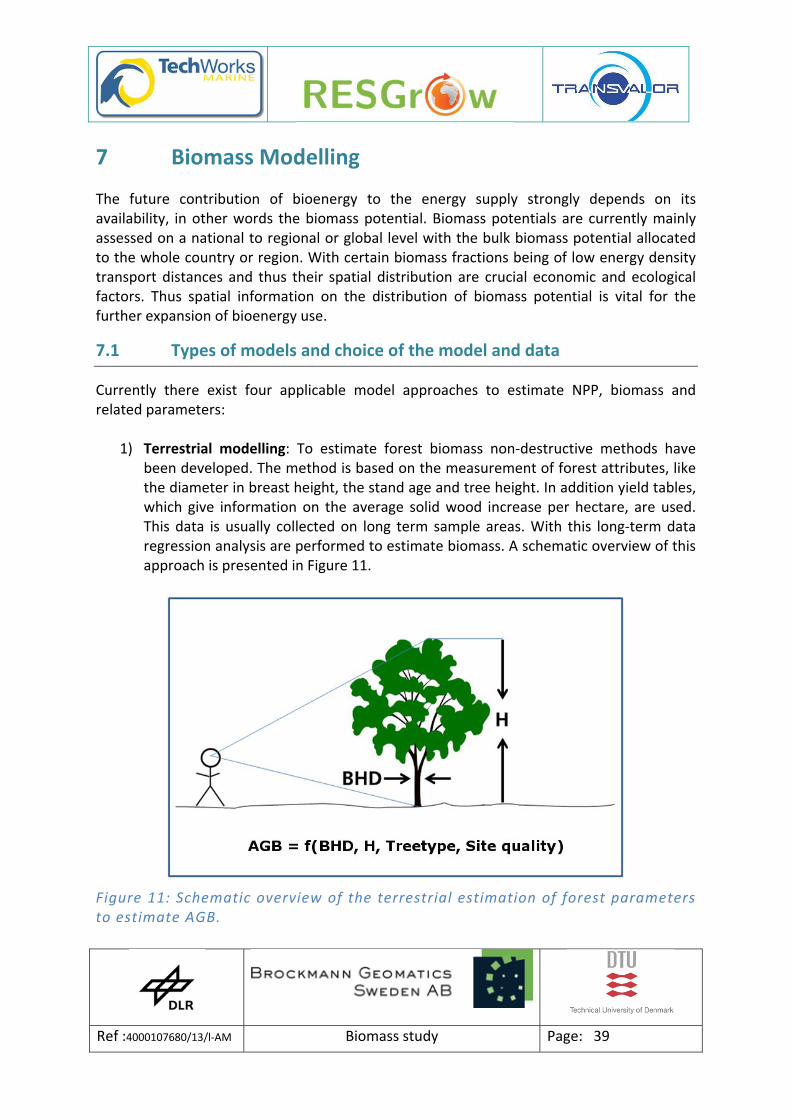
1) Terrestrial modelling: To estimate forest biomass non‐destructive methods have been developed. The method is based on the measurement of forest attributes, like the diameter in breast height, the stand age and tree height. In addition yield tables, which give information on the average solid wood increase per hectare, are used. This data is usually collected on long term sample areas. With this long‐term data regression analysis are performed to estimate biomass. A schematic overview of this approach is presented in Figure 11.
Figure 11: Schematic overview of the terrestrial estimation of forest parameters to estimate AGB.

Ref :4000107680/13/l‐AM Biomass study Page: 40
2) Empirical estimates with help of remote sensing: Empirical models are based on
statistical relationships between yield and environmental parameters, which can be derived using various techniques of remote sensing. Many statistical approaches have been developed during the last years which link e.g. EO data to crop yields. In addition so called vegetation health indices (VH) have been developed to link temperature and water stress to satellite signals.
3) Mechanistical models: Mechanistical models, often also called “Production Efficiency Model (PEM)” describe the temporal change of biomass in a simplified way. Here mainly the light energy controls vegetation growth, assuming photosynthesis, modelled after Monsi and Saeki (1953) and Monteith (1965), is linearly related to the absorbed PAR. A schematic overview of the general approach is presented in Figure 12.
Figure 12: Schematic overview of PEM models.
4) Dynamic and SVAT models: Dynamic models and Soil‐vegetation‐atmosphere‐
transfer (SVAT) models describe bio‐physical and bio‐chemical processes explicit and quantitative. Interactions of Vegetation, Atmosphere and Pedosphere are regarded, also including processes like the water cycle. Photosynthesis is calculated following the approaches of Farquhar et al. (1980) and Collatz et al. (1992). A schematically overview is presented in Figure 13.

Ref :4000107680/13/l‐AM Biomass study Page: 41
Figure 13 Scheme of interactions regarded in dynamic and SVAT models.
To guide the choice of which modelling approach is most suitable for application, the following questions should be answered:
Which values should be estimated (e.g. crop yield or potential energy output)?
At which time yield forecasts have to be available?
Which precision of the forecasts is necessary?
Which kinds of input data shall be used? The applied data are limited due to their costs and the time at which they are available.
Which effort in data processing and data management is accepted?
Which spatial coverage is necessary and can the method be adapted to other regions? The spatial resolution of input data is dependent on the scale at which the simulations shall take place.
Is the forecast objective, transparent and reproducible
7.2 Overview of institutions existing models
This chapter will shortly introduce some of the exiting vegetation models and their applications and gives reference to more detailed information. The sorting follows alphabetical order.
7.2.1 AGROSIM

Ref :4000107680/13/l‐AM Biomass study Page: 42
At the Center for Agricultural Landscape and Land Use Research, Institute for Landscape Systems Analysis, in Eberswalde (Germany) the agro ecosystem model family AGROSIM was developed for simulating the yield of homogeneous crop stands (winter wheat, winter barley, winter rye and sugar beet) under field conditions for limited and unlimited water and nitrogen supply (Mirschel et al., 1995). All models only need meteorological standard values as driving forces and regional available inputs and parameters. The AGROSIM models base on the same modelling philosophy, have a similar model structure on the basis of modules (meteorology, plant soil), use rate equations for describing process dynamics as e.g. photosynthesis, respiration, transpiration, dry matter allocation and root growth, calculate on a minimum time step level of one day and are weather, site and management sensitive. In all models the plant growth module active interacts with a soil process module. One of the most important sub processes within AGROSIM models is the process of ontogenesis (biological time scale) which acts as a time‐related control variable on other sub processes. Other processes are initiated, stopped, accelerated or slowed down by ontogenesis. The second important sub process within AGROSIM models is the photosynthesis which acts as the source of daily biomass production. The daily assimilation rate bases on a maximum photosynthetic rate per unit green biomass and is influenced by water and nitrogen stress. The soil processes are based on daily calculations for soil layers up to 2 meters. In recent time, AGROSIM was coupled with hyper‐spectral, high‐resolution remote sensing data (HyMapTM data) within a model‐GIS structure. Regional yield estimation for winter wheat and sugar beet within a test side of about 65 square kilometres in the Uckermark region were calculated and validated with site‐specific in‐situ data. Deviation from measured data of less than 20% could be achieved for all investigated sites (Wegehenkel et al., 1999).
7.2.2 BETHY/DLR The German Remote Sensing Data Center (DFD) is operating the SVAT model BETHY/DLR (Biosphere Energy Transfer Hydrology Model) to estimate the Net Primary Productivity (NPP) of agricultural and forested areas. It was developed by Knorr and Heimann (2001) and further expanded by Wisskirchen (2005) and Tum (2012). The model is driven by remote sensing data and meteorological data. As remotely sensed datasets time series about the Leaf Area Index (LAI), which describes the condition of the vegetation, and a land cover classification, which provides information about the type of land use, are needed. Currently the LAI time series and the land cover (GLC2000) are derived from the sensor VEGETATION are used. Both data have spatial resolutions of about 1 km x 1 km and are freely available globally. Furthermore monthly averages of CO2 concentration derived from the GOSAT sensor. This dataset is available on a 2.5° x 2.5° global grid.

Ref :4000107680/13/l‐AM Biomass study Page: 43
The meteorological input parameters, which are as the air temperature at 2m height, precipitation, cloud cover and wind speed at 10m above ground, are derived from the European Centre for Medium range Weather Forecast (ECMWF). They have a spatial resolution of about 0.25° x 0.25° and a temporal resolution of up to four times a day. The NPP output of BETHY/DLR has been used to estimate e.g. the sustainable energy potential of agriculture and forest areas in Europe. For this conversion factors of the above to below ground biomass, the carbon and water content and lower heating values were applied. A detailed description of this approach is presented in Tum et al. (2011) and Tum et al. (2013). An example of the sustainable straw potential is presented in Figure 14.
Figure 14: Sustainable straw potential for 2010.
7.2.3 CERES and DSSAT The daily growth of plants is modelled in CERES according to the Radiation Use Efficiency (RUE) approach, which is based on the concepts of Monsi and Saeki (1953) and Monteith (1965). In this approach, the potential maximum dry matter production is linearly correlated with the absorbed light. As in most mechanistic models, RUE also varies with temperature,

Ref :4000107680/13/l‐AM Biomass study Page: 44
nitrogen and water availability, CO2 level and fertilization. The allocation of assimilated carbon to particular plant components is modelled, with daily time steps. Phenology, the timing of biological processes, is driven by temperature, expressed as either thermal temperature or growing‐degree‐days. In order to calibrate the CERES model, field data are needed, especially the number of plants planted per unit area and the timing of phonological events such as tilling, stem elongation, and maturation. Grain yield metrics are also mandatory. The CERES model is now integrated in the Crop Simulation Model (CSM) of the Decision Support System for Agrotechnology Transfer (DSSAT) distributed by the International Consortium for Agricultural Systems Applications in Honolulu (Jones and Kiniry, 1986). In its earliest form the DSSAT model was developed to simulate maize growth and development, but in the DSSATCSM, 27 different cropping system models are combined. At a minimum, it needs input data regarding incoming solar radiation, minimum and maximum temperatures, and rainfall. It can additionally utilize several soil‐related metrics, such as bulk density, carbon content, and pH, as well as management‐related metrics such as planting density, fertilization rates and irrigation data. Another important crop growth
7.2.4 DNDC Another important crop growth model is the DeNitrification and DeComposition (DNDC) model, originally developed by Li et al. (1992). In DNDC, crop growth is parameterized by generalized crop growth curves together with a crop‐specific potential maximum grain yield. The actual grain yield is determined by the availability of nitrogen in the soil. Nitrogen uptake by the plants is controlled by the soil temperature profile and soil moisture. With this approach, the effects of differences in tilling, fertilizer use and irrigation can be taken into account by DNDC, because all of these management practices modify the soil regime and thus affect plant growth. DNDC also integrates crop growth processes with biogeochemical processes by including important nitrogen‐ and carbon related processes like mineralization, ammonia volatilization, denitrification and nitrification, nitrogen uptake and leaching. The DNDC model, presently implemented with a daily time step, has been validated and used for many subnational and national case studies (e.g.: Stange et al., 2000, Cai et al., 2003).

Ref :4000107680/13/l‐AM Biomass study Page: 45
7.2.5 ECGM
The EARS Crop Growth Model (http://www.ears.nl/crop_yield_forecasting.php) is developed by EARS (Environmental Analysis & Remote Sensing), a remote sensing company in the Netherlands. One of the activities is crop yield forecasting in Africa, China and Europe. Crop yield forecasting is based on a crop growth model, which uses the satellite derived radiation and actual evapotranspiration data as input. The model is based on the observation by Monteith (1977), that all crops have about the same growth rate per unit leaf area and that differences in production can be explained by differences in crop geometry and corresponding light interception. This model was extended to include the effects of drought and photosynthetic efficiency.
Crop growth conditions are characterized by the relative evapotranspiration during the month passed, which is the average actual evapotranspiration divided by the average net radiation. They are both derived from METEOSAT noon and midnight images in the visible and thermal infrared, by means of EARS‐EPS, the energy balance processing system. The relative evapotranspiration is a measure of water availability to the crop. It can be considered equal to the relative growth of a wheat crop under water limitation.
Crop growth is simulated on the basis of a dedicated crop growth model, which is fed with the distributed radiation and actual evapotranspiration data generated by the EARS‐EPS. In this way the estimated crop biomass is obtained at the end of each month. With the same model the potential biomass is obtained assuming no water limitation. The ratio of the actual to the potential biomass is called the crop yield indicator. Two to three months after the beginning of the growing season it gives a good forecast of the end of season relative yield. A product example is given in Figure 15.

Ref :4000107680/13/l‐AM Biomass study Page: 46
Figure 15: Sorghum/millet Difference Yield forecast for the Horn of Africa, starting from the first decade of July until the last decade of September 2007. The forecast early July and early August do predict the end of season result (Sept D3) quite well. Source: http://www.ears.nl/crop_yield_forecasting.php
7.2.6 EPIC In the early 80s of the last century, the Erosion Productivity Impact Calculator (EPIC) was developed by a modelling team of the USDA to assess the status of U.S. soil and water resources (Williams, 1995). Since that time EPIC has been continuously expanded and refined to allow simulation of many processes important in agricultural land management resulting in renaming the model to Environmental Policy Integrated Climate (EPIC) model. The new EPIC model now includes carbon cycling routines and the emission of greenhouse gases (e.g. N2O, CH4). The major components in EPIC are weather simulation, hydrology, erosion‐sedimentation, nutrient and carbon cycling, pesticide fate, plant growth and competition, soil temperature and moisture, tillage, cost accounting, and plant environment control. EPIC operates on a daily time step and can simulate plant growth for hundreds of years. The spatial resolution of EPIC is adjusted to the field size (Homogeneous Response Unit, HRU) assuming that weather, soil, topography, and management systems are homogeneous. Heterogeneous landscapes can be modelled by identifying a reasonable

Ref :4000107680/13/l‐AM Biomass study Page: 47
number of representative homogenous HRUs. A schematic set‐up of EPIC is shown in Figure 16. The input data for EPIC are weather (precipitation [mm], minimum and maximum air temperature [°C], and solar radiation [MJ/m²]), physical and chemical soil parameters describing the soil layer with depth, topography (field size [ha], slope length [m] and steepness [%]) and management practices (e.g. planting day, harvesting day, harvesting index, date and depth of each tillage operation, scheduling options for timing and rate of irrigation water, fertilizer, lime, pesticide, grazing, and drainage systems).
Figure 16: Schematic set‐up of data processing and information flow of EPIC. Source: Schneider et al., 2009.
7.2.7 FAO
FAO's mandate is to raise levels of nutrition, improve agricultural productivity, better the lives of rural populations and contribute to the growth of the world economy. FAO uses a so called AEZ agro‐ecological zones methodology model approach in order to achieve information about potential crop yields.

Ref :4000107680/13/l‐AM Biomass study Page: 48
Over the past twenty years, the term agro‐ecological zones methodology (AEZ) has become widely used (Fischer et al. 2000). However, it has been associated with a wide range of different activities that are often related yet quite different in scope and objectives. FAO and the International Institute for Applied Systems Analysis (IIASA) differentiate the AEZ methodology in the following activities: First, AEZ provides a standardized framework for the characterization of climate, soil and terrain conditions relevant to agricultural production. In this context, the concepts of Length of Growing Period (LGP) and of latitudinal thermal climates have been applied in mapping activities focussing on zoning at various scales, from sub‐national to global level. Second, AEZ matching procedures are used to identify crop‐specific limitations of prevailing climate, soil and terrain resources, under assumed levels of inputs and management conditions. This part of the AEZ methodology provides estimates of maximum potential and agronomical attainable crop yields for basic land resources units. Third, AEZ provides the frame for various applications. The previous two sets of activities result in very large databases. The information contained in these data sets form the basis for a number of AEZ applications, such as quantification of land productivity, extents of land with rain‐fed or irrigated cultivation potential, estimation of the land’s population supporting capacity, and multi‐criteria optimization of land resources use and development. The AEZ methodology utilizes a land resources inventory to assess, for specified management conditions and levels of inputs, all feasible agricultural land‐use options and to quantify expected production of cropping activities relevant in the specific agro‐ecological context. The characterization of land resources includes components of climate, soils and landform. Recent availability of digital global databases of climatic parameters, topography, soil and terrain, and land cover has allowed for revisions and improvements in calculation procedures and to expand assessments of AEZ crop suitability and land productivity potentials to temperate and boreal environments. This effectively enables global coverage for assessments of agricultural potentials.
For practical purposes, FAO intends to continue work on the two main components of bioenergy: wood energy and agro‐energy. The Forestry Department will continue to take the lead on wood energy and the Sustainable Development Department on agro‐energy. Areas of work with potential for improved collaboration include:
statistics on wood and agro‐energy; biofuels resources and supply/demand outlook; information on energy from crops, residues and wastes; bioenergy for rural industries, specially food industries; analysis of competition between raw materials for food, fuels and other uses; cost‐benefit analyses of the various forms of bioenergy production both from the
producers and ’the overall society’s perspectives; assessments of the potential and the impacts of a monetization of positive external
effects, particularly for developing countries;
Ref :4000107680/13/l‐AM Biomass study Page: 49
analyses of possible impacts on food prices and availability associated with a growing use of land, water and other agricultural resources for bioenergy production, particularly for poor, food and energy importing countries;
energy and climate change and carbon balances; trade in biofuel; information on bioenergy policies, institutional and legal aspects; technical, economic, social and environmental aspects of bioenergy systems; and land tenure and other socio‐economic issues, including rural livelihoods, gender and
farming systems.
7.2.8 G4M The Global Forest Model (G4M), developed at IIASA (Kindermann et al., 2013), predicts the annual above ground wood increment and stocking biomass. The Global Forest Model was developed to decide if afforestation or deforestation of a managed forest area can result in a higher income than alternative land use on the same place. Therefore, the income of managed forest (difference of wood price and harvesting costs, income by storing carbon in forests) is compared to the income of alternative land use. G4M needs a yield description as an input parameter as e.g. the net primary productivity (NPP) for a certain species at a specific region. The NPP can be supplied by NPP‐maps or by models. Currently the species beech, birch, fir, larch, oak, pine and spruce are parameterised. The model can estimate the current rotation time assuming a normal forest out of a biomass map and a given yield. It is also possible to use observed age structures to initialize a forest. As management it's possible to select a target rotation time, if thinning is done or not and which species are regenerated. It's also possible to let the model chose the rotation time by own with the task to either have the highest wood growth rate or to have the highest biomass in the forest. Currently in development is to include an estimate of forest fire risk and a management option to react on this risk like shorter rotation time and lower stand densities in case of fire risk. As G4M is spatially explicit (currently on a 0.5°x0.5° resolution grid which is planned to bring down to 30"x30") the different deforestation pressure at the forest frontier can also be handled.
7.2.9 IBSAL
The Integrated Biomass Supply Analysis & Logistics (IBSAL) Model is developed at Oak Ridge National Laboratory (ORNL) with support from the Office of Biomass Programs. The IBSAL Model is made of a network of operational modules and connectors threading the modules. Each module represents a process or event. For example grain combining, swathing grasses, baling, grinding and sizing, storing, transporting are each a module. Modules may also be processes such as drying, wetting, and chemical reactions such as breakdown of
Ref :4000107680/13/l‐AM Biomass study Page: 50
carbohydrates. Costing and energy calculations common to all operations are gathered into individual modules as well. Each module is independently constructed as a black box with a set of inputs and outputs. The module may also interact with an external EXCEL spread sheet to receive data from or write data to. The biomass flows from one module to the next through a connector. The time the biomass spends in the system is determined by the modules and not by the connectors.
A typical model starts from defining the logistical features of the supply such as number of farms involved, average yield, the start and progress of harvest schedule, and the moisture content of the crop. The model also requires daily weather data such as temperature, relative humidity, wind speed, rainfall and snow fall. A spread sheet containing equipment specifications provides data for calculating service times. This information is used in calculating drying and wetting of the biomass and workability of the soil. The user also defines the safe moisture content for baling and minimum temperature below which farm operations will cease. Once all input parameters are identified, the model calculates costs per ton of biomass, energy input and emissions (CO2) from equipment.
7.2.10 MARS The aim of the European Commission when starting the 10 year project "Monitoring Agriculture with Remote Sensing" (MARS / STAT) in 1988 was (Council decision 88/503/EEC of 26 September 1998)
to improve and harmonise European agricultural statistics using a range of new methods notably remote sensing and
to produce regular crop status bulletins by the Integrated Agricultural Information System (IAIS) providing early statistical information about crop surfaces and potential yields to the Directorate General of Agriculture (DG VI) and to EUROSTAT, the European Statistical Office.
The regional inventories were designed to meet the need for accurate and objective annual information on acreage at regional level covering the main crops by establishing close links between satellite data and observations on the ground. In parallel objective observations in the field (ground truth) with a sample design established or enhanced by remote sensing, with full coverage of the region with SPOT or LANDSAT images were performed. For the ground survey, the basic unit is a 700 m x 700 m square named "segment". The segments of the sample are located and drawn on maps and aerial photographs, and then visited. Agronomic information per field (e.g. farming practice, sowing, planting and harvesting date, plant density, variety, soil type, irrigation, species...) were added as well as qualitative appreciation of the status of the crops (Figure 17).

Ref :4000107680/13/l‐AM Biomass study Page: 51
Figure 17: The MARS yield forecast system
Most of the activities in the MARS project are the continuation of existing activities that were previously known under names like MARS‐STAT, for area statistics and yield monitoring, and MARS‐PAC, for all activities related to the implementation of the Common Agricultural Policy. These activities have a strong regulatory basis as they are linked to specific requests from DG VI and the member states. http://www.marsop.info/marsop3/
The MARS Project has developed, tested and implemented new methods and tools specific to agriculture using remote sensing. The project is divided into four main activities:

Ref :4000107680/13/l‐AM Biomass study Page: 52
Anti fraud measures: This is, in fact, a multifaceted activity, with measures to combat fraud related to the implementation of the CAP as central theme. Tasks include the management of the control with remote sensing program, and related quality checks, tests and further developments of evaluation methods, land parcel identification systems and collection of production statistics of vineyards and olive trees, as well as support to the management of agro environmental subsidies.
Crop and yield monitoring: crop yield monitoring with agro‐meteorological models and low resolution remote sensing methods and area estimates using high resolution data combined with ground surveys.
Specific surveys: application of area frame sampling techniques to provide rapid and specific information needed for the definition or reform of agricultural policies
New Sensors and methods: following technological developments in new sensors, precision farming techniques and alternative data collection and processing techniques for large scale agricultural applications
The crop and yield activity is structured along the following activities:
Agro‐meteorological models (Crop Growth Monitoring System ‐ CGMS) Low resolution remote sensing methods Area estimates using high resolution data combined with ground surveys
The results of the yield monitoring activities are synthesized as the MARS Bulletin, a report published regularly through the European growing season which include:
Full Analysis is published from 6 to 8 times a year on European Crop Monitoring and Yield Forecasting. These publications are also available on request in paper format.
Quick Look releases (i.e. shorter digital versions or e‐mail versions) of the same analyses are available to facilitate downloading and are loaded in the site before the final full analysis.
Climatic Updates are brief intermediate analyses between two main bulletins and are available only in digital version.
The Crop Growth Monitoring System developed by MARS Project provides the European Commission (DG Agriculture) with objective, timely and quantitative yield forecasts at regional and national scale. CGMS monitors crops development in Europe, driven by meteorological conditions modified by soil characteristics and crop parameters. This mechanistic approach describes crop cycle in combination with phonological development from sowing to maturity on a daily time scale. The main characteristic of CGMS lies in its specialisation component, integrating interpolated meteorological data, soils and crops parameters, through elementary mapping units used for simulation in the crop model WOFOST.

Ref :4000107680/13/l‐AM Biomass study Page: 53
7.2.11 Further models approaches The following Table 4 gives an overview of further models, which have been used to estimate above ground biomass and/or NPP. A good overview is also given in Fatoyinbo, 2012. An interesting comparison of eight widely used, easily accessible and well‐documented crop growth models for winter wheat can be found in Palosuo et al. (2011). The authors simulated winter wheat yields and its variability in different climates of Europe for 49 growing seasons. They found that “none of the models perfectly reproduced recorded observations at all sites and in all years, and none could unequivocally be labelled robust and accurate in terms of yield prediction across different environments and crop cultivars with only minimum calibration.” But they also summarized that “the mean model predictions were in good agreement with observed yields.”
Table 4: Models to estimate above ground biomass / NPP. The nomenclature of references is as follows: First author, Journal abbreviation (see footnote below table), Issue, Pages, Year.
Model Sensor Dynamic input
data Spatial
resolution Landcover R2 Sources
C-Fix (det) VGT NDVI 1km x 1km All LCLU
Classes
Veroustrate_RSE_83_376-399_2002
EARS-CGS (det)
Meteosat; MSG; FY-
2
LST, Cloudiness,
AOT
>3km x 3km
All LCLU Classes
0.72 – 0.94
(NUTS)
Roebeling_IJRS_25_5389-5401_2004
RBM (det) MODIS NDVI, LST, water vapour
deficit 1km x 1km Agriculture 0.82
Richters_Thesis_2005
VPM (det) MODIS;
VGT NDWI, EVI,
NDVI 1km x 1km
Tropical forest
0.32 - 0.61
Xiao_RSE_94_105-122_2005
Simplified BIOME-BGC (MOD17) (det)
MODIS LCC, LAI 1km x 1km All LCLU
Classes 0.77
Zhao_RSE_95_164-176_2005
BETHY/ DLR (dyn)
AVHRR VGT
LCC, LAI 1km x 1km All LCLU
Classes 0.61 – 0.86
Wißkirchen_Thesis_2005; Tum_BB_35_4665-4674_2011
Miami-Modell (det)
-
Temperature, Precipitation,
Annual evapotranspirati
on
4 zones Forest and Agriculture
Lieth_SpingerVerlag_1975
TREEDYN3 (det)
- Location, Time, average annual
temperature Forest
Bossel_EM_90_187-227_1996

Ref :4000107680/13/l‐AM Biomass study Page: 54
Biome/Forest-BGC (det)
- Yield table,
Met. data, LCC Stock Forest
Running_TP_9_147-160_2004; White_EI_4_1-85_2000
PnET_model family (det)
- Met. data Stock Forest > 0.8 Aber_O_92_463-474_1992
EPIC (det) - LCC 10km x
10km und 1km x 1km
Agriculture Williams_TASAE_27_129-144_1994
G4M (det) - Yield table, NPP, LCC
1km x 1km Forest 0.43 – 0.75
Kindermann_CBM_8:2_2013
FORUG (det) - Met. data, LAI,
LCC Stock Forest
0.67 - 0.85
Verbeeck_EC_210-85-103_2008
FORGRO (dyn)
- Forest
parameter 1ha x 1ha Forest Mohren_Thesis_1987
3-PG (dyn) - Met. data, LCC, LAI (optional)
Stock Forest > 0.9 Landsberg_FEM_95_209-228_1997
BALANCE (dyn)
- Met. data, LCC Stock,
single trees Forest > 0.81
Grote_PB_4_167-180_2002
CASTANEA (dyn)
- Met. data, LCC Stock Forest 0.88 Dufrêne_EM_185_407-436_2005
ORCHIDEE (dyn)
- Met. data, LCC 0.25° x 0.25°
All LCLU Classes
0.47 - 0.93
Krinner_GBC_19_2005; Abramowitz_JC_21_5468-5481_2008
FORUG (dyn)
- Met. data, LAI,
LCC Stock,
single trees Forest
0.69 - 0.87
Verbeeck_EC_210-85-103_2008
SILVA (hybrid)
-
Site characteristics, tree condition
(crown), spatial structure
Stock Forest Pretzsch_FEM_162_3-21_2002
7.3 Empirical estimation of biomass potentials using remote sensing
In the following chapter results of today’s experimental and operational remote sensing based methods to estimate biomass potentials will be described. Most methods base on the general approach to correlate remote sensing products with in situ measurements or estimations of biomass, its yield or plant specific parameter as e.g. the diameter in breast height (BHD). Experimental methods usually consist of methods, which in principle show, that biomass can directly be derived using remote sensing data. These approaches however, have been applied for few time steps and regions only. Investigation showed that these experimental approaches often deliver, compared to operational methods, products with higher spatial and temporal resolution, with also a higher level of accuracy. Operational methods however, provide biomass maps for larger areas (national, continental up to global) and longer time series.
Ref :4000107680/13/l‐AM Biomass study Page: 55
In literature many approaches of experimental approaches to correlate measurements of optical and microwave sensors with above ground biomass can be found (see Table 5). The highest coefficient of determination with r² = 0.96 was found for biomass in Spanish forests, which was derived using an average annual NDVI (Gonzales‐Alonso et al. 2006). To derive NDVI they used data from the French Sensor VEGETATION, installed on the SPOT satellite, which has a spatial resolution of approximately 1km x 1km. VEGETATIN is a multi‐spectral sensor with 4 channels. As NDVI represents a vegetation parameter which is widely used to monitor the greening condition of vegetation, it can be correlated with biomass. Other approaches which are based on the use of sensors with higher spatial resolution as e.g. Enhanced Thematic Mapper (ETM+) on Landsat 7 (30m x 30m resolution) revealed comparable results (Zheng et al. 2004). However, a major shortcoming of these approaches lies within the lack of possibility of easy transferability to other regions. Thus to estimate above ground biomass for other forest areas with different tree species, growing conditions and age structure, these experimental approaches need to be basically reinvented from start. Also active systems, like Light detection and ranging (Lidar) and Radio detection and ranging (Radar) have been used. With Radar the intensity and polarization of the backscatter signal is measured and correlated with above ground biomass. Here the relationship between backscatter (intensity and depolarization) and canopy structure is used. High correlative results show investigations done with the Radar system SIR‐C (Spaceborne Imaging Radar using the C‐Band), which however was used only for an 11 day experiment in April 1994 at the American Space Shuttle (Bergen and Dobson 1999). The wavelength of a C‐band Radar is at approximately 5 cm and thus within the range of smaller tree branches, which thus contribute at maximum to the backscatter signal. Further investigation with Radar sensors using various wave lengths and spectral resolutions prove the high correlation of backscatter signal and above ground biomass. Thus in 2013 the European Space Agency (ESA) launched the “Biomass” mission as the seventh Earth‐Explorer‐Mission. Its aim will be to measure the intensity of the backscatter and depolarization of a Radar signal, to monitor biomass of thicker branches and the stem of forests. Start of “Biomass” is foreseen to be in 2020 (ESA 2012). First tries to install and use Laser instruments onboard aircrafts to work on forest biomass monitoring were performed in the early 80s (Nelson et al. 1984). These so called Lidar systems are comparable to Radar systems, however the wavelength of Laser scanners lays within the bandwidth of near infrared (~ 1µm). With Lidar the distance between aircraft and tree canopy and aircraft and ground is measured. With this approach the tree height can be calculated. Using auxiliary information like tree species, tree age it is possible to estimate above ground biomass. The Geoscience Laser Altimeter System (GLAS) onboard of ICESat (Ice, Cloud and land Elevation Satellite) has been used to produce a map, showing the above ground biomass of forests (Pflugmacher, 2007). ICESAT was originally planned to monitor the polar ice thickness. Every 150 meters GLAS measures the Earth surface at Nadir with a
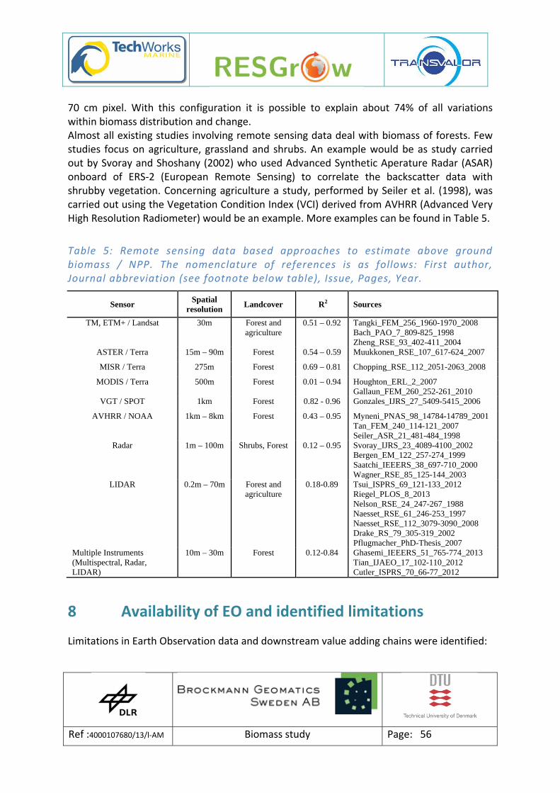
Ref :4000107680/13/l‐AM Biomass study Page: 56
70 cm pixel. With this configuration it is possible to explain about 74% of all variations within biomass distribution and change. Almost all existing studies involving remote sensing data deal with biomass of forests. Few studies focus on agriculture, grassland and shrubs. An example would be as study carried out by Svoray and Shoshany (2002) who used Advanced Synthetic Aperature Radar (ASAR) onboard of ERS‐2 (European Remote Sensing) to correlate the backscatter data with shrubby vegetation. Concerning agriculture a study, performed by Seiler et al. (1998), was carried out using the Vegetation Condition Index (VCI) derived from AVHRR (Advanced Very High Resolution Radiometer) would be an example. More examples can be found in Table 5.
Table 5: Remote sensing data based approaches to estimate above ground biomass / NPP. The nomenclature of references is as follows: First author, Journal abbreviation (see footnote below table), Issue, Pages, Year.
Sensor Spatial
resolution Landcover R2 Sources
TM, ETM+ / Landsat 30m Forest and agriculture
0.51 – 0.92 Tangki_FEM_256_1960-1970_2008 Bach_PAO_7_809-825_1998 Zheng_RSE_93_402-411_2004
ASTER / Terra 15m – 90m Forest 0.54 – 0.59 Muukkonen_RSE_107_617-624_2007
MISR / Terra 275m Forest 0.69 – 0.81 Chopping_RSE_112_2051-2063_2008
MODIS / Terra 500m Forest 0.01 – 0.94 Houghton_ERL_2_2007 Gallaun_FEM_260_252-261_2010
VGT / SPOT 1km Forest 0.82 - 0.96 Gonzales_IJRS_27_5409-5415_2006
AVHRR / NOAA 1km – 8km Forest 0.43 – 0.95 Myneni_PNAS_98_14784-14789_2001 Tan_FEM_240_114-121_2007 Seiler_ASR_21_481-484_1998
Radar 1m – 100m Shrubs, Forest 0.12 – 0.95 Svoray_IJRS_23_4089-4100_2002 Bergen_EM_122_257-274_1999 Saatchi_IEEERS_38_697-710_2000 Wagner_RSE_85_125-144_2003
LIDAR 0.2m – 70m Forest and agriculture
0.18-0.89 Tsui_ISPRS_69_121-133_2012 Riegel_PLOS_8_2013 Nelson_RSE_24_247-267_1988 Naesset_RSE_61_246-253_1997 Naesset_RSE_112_3079-3090_2008 Drake_RS_79_305-319_2002 Pflugmacher_PhD-Thesis_2007
Multiple Instruments (Multispectral, Radar, LIDAR)
10m – 30m Forest 0.12-0.84 Ghasemi_IEEERS_51_765-774_2013 Tian_IJAEO_17_102-110_2012 Cutler_ISPRS_70_66-77_2012
8 Availability of EO and identified limitations
Limitations in Earth Observation data and downstream value adding chains were identified:

Ref :4000107680/13/l‐AM Biomass study Page: 57
Land cover classification (LCC) databases typically do not distinguish between different energy crops or list only a small subset of them.
The moisture content of energy crops is not modelled.
Net primary productivity (NPP) is provided operationally by NASA and planned for by ESA, but not for different energy crops. Actual land cover classification is missing to extend NPP modelling.
Therefore, spatial and temporal variability of the bioenergy resources is difficult to assess with the help of EO data in this case. Only experimental information restricted to a few crops based on a study level are available.
For forests, an initial database of biomass for a reference year is needed as NPP modelling provides only a yearly increment to be added to a reference year.
For forests, additionally information about the age of a tree population is needed to choose appropriate allocation rules for the estimation of trunk volume growth as a function of NPP.
Due to the limitations identified above for an high spatial resolution and actual biomass assessment, research groups and industries from the energy sector typically rely on biomass potentials based on statistical yield data of different energy crops. Such statistical data is typically available as an average value for a larger region or on the country level. As the supply radius of bioenergy power plants is typically much smaller, a gap in information occurs. Secondly, inter‐annual variability is typically not taken into account. Therefore, further disaggregation of such statistical data based on geophysical parameters is needed. So far, JRC and DLR used land cover classification, leaf area index, radiation and meteorological parameters for net primary productivity derivation as a basis for disaggregation. These are examples for the use of EO information for biomass potential assessment. However these limitations might be at least to some extend lowered with the possibilities the forthcoming Sentinel missions and the Biomass mission in special. Fehler! Verweisquelle konnte nicht gefunden werden. summarises the potential of applying Earth Observation based information for the management of the biomass energy resource.

Ref :4000107680/13/l‐AM Biomass study Page: 58
Table 6: Potential for remote sensing data use in the life cycle of a bioenergy power plant.
Needs for Potential of EO use
Status of EU use
Feasibility study / Potential analysis
Large scale resource assessment
High Experimental for few crops
Vegetation monitoring High Established but gaps
Land use information High Established but gaps
Site selection Regional resource assessment
High Experimental for few crops
Vegetation monitoring High Established but gaps
Land use information High Established but gaps
Digital elevation model High Established
Permit stage Register databases Medium Established
Environmental impact Medium To be tested
Design & Engineering
Logistics Medium To be tested
Variability information High Experimental for few crops
Construction Infrastructure information High Established
Operation & Maintenance
Logistics Medium To be tested
Trading High To be tested
Yield monitoring High Established but gaps
Decommissioning No specific needs
8.1 Biomass potentials
There exists a variety of methods on the derivation of above‐ground‐biomass (AGB) from remote sensing data. The review paper by Lu (2006) gives an excellent overview on different approaches tested in several regions, for different crops and forest types and with a variety of different sensors. Overall, model transferability is often a major point of interest in model development, but in reality it is difficult to directly transfer one model to different study areas because of limitation of the model and the remotely sensed data.’ Therefore, general approaches suitable for large area mapping seem to be still an issue of on‐going research. Some citations on problems frequently observed are given here:
Fine spatial resolution data (up to 10 m resolution): one important application may be its use as reference data for validation or accuracy assessment for medium and coarse spatial‐resolution data applications. The drawback is that the high spectral variation and shadows caused by canopy and topography may create difficulty in developing AGB estimation models. Another drawback is the lack of a shortwave

Ref :4000107680/13/l‐AM Biomass study Page: 59
infrared image, which is often important for AGB estimation. Also, the need for large data storage and the time required for image processing prohibit its application in large areas. Last but not least, high spatial resolution imagery is much more expensive, and requires much more time to implement data analysis than medium spatial resolution images.’
Medium spatial resolution data (10 – 100 m resolution): not all vegetation indices are significantly correlated with AGB. In practice, it is still difficult to identify which texture measures, window sizes, and image bands are suitable for a specific research topic, and the lack of a guideline on how to select an appropriate texture further complicates the process.’
Coarse spatial resolution data (> 100 m resolution): ‚Overall, the AGB estimation using coarse spatial‐resolution data is still very limited because of the common occurrence of mixed pixels and the huge difference between the size of field‐measurement data and pixel size in images. A synthetic analysis of multi‐scale data with a combination of different modelling approaches may be needed for AGB estimation in a large area.’
Radar data: ‚The saturation problem is also common in radar data. The saturation levels depend on the wavelengths, polarization, and the characteristics of vegetation stand structure and ground condition.’
‚radiometric and atmospheric correction is an important but difficult task’ Due to the lack in methods suitable for an overall biomass assessment, research groups and industries from the energy sector typically rely on biomass potentials based on statistical yield data of different energy crops. Such statistical data is typically available as an average value for a larger region as an administrative district or on the country level. As the supply radius of bioenergy power plants is typically much smaller, a gap in information occurs. Also, the temporal resolution of such databases is inadequate as they often refer to a single reference year. Inter‐annual variability is not taken into account. Therefore, further disaggregation of such statistical data based on further geophysical parameters is needed. JRC uses land cover classification and DLR uses land cover classification, leaf area index, radiation and meteorological parameters for net primary productivity derivation as a basis for disaggregation.
8.2 Land cover classification
For biomass resource assessment a unit of tons per hectare biomass yield is needed for each energy crop of interest. A fundamental question is where each energy crop type is grown.

Ref :4000107680/13/l‐AM Biomass study Page: 60
An optimum data base would be a satellite‐based land cover classification with an update each year with a classification legend distinguishing between the different energy crops. A spatial resolution of few hundred meters or would be sufficient, but a better resolution would be of help. For a general overview (e.g. continental or global assessment) a resolution up to 1 km can also be used. The range of projects, programs, and organisations that use land cover data to meet their planning, management, development and assessment objectives has expanded significantly. In general, land use ‐ / land cover data are needed for inventory purposes as classification of vegetation type, canopy closure, wildlife habitat, urban development, agricultural land use, damage from natural hazards and snow‐pack for water supply. In the moment a lot of modelling activities begin which need as basic input knowledge about land use / land cover and soil characteristics. Examples are modelling irrigation depletion and drought forecast, fire danger assessment, risk of disturbance, flooding within suitable catchments, landslide forecast and risk assessment, urban growth, forecast of coastal storms, climate effects and global change. Despite the high demand of natural resources information, many existing maps (also in digital format) are not developed to really meet multi ‐ user requirements. One of the basic causes of such a situation is the type of classification / legend used to describe basic information as land cover and / or land use depends on the spatial resolution. From a remote sensing point of view, a (spatial) high resolution sensor with 1 x 1 m2 pixel size will give detailed information about e.g. single trees (which might be classified) while sensors with a resolution like MERIS (300 m x 300 m pixel size) gives information on forests rather than trees. The spatial resolution of a land use / land cover map is also interesting from the user’s point of view. Climatologists working in the field of global weather forecast are more interested in general classes as e.g. forest or arable land than in detailed information about regional or local features as maize or wheat fields. Global land cover / land use maps are typically scaled to 1:2,000,000 supporting national operational programs global change research, international studies and global climate modelling. For regional applications as e.g. regional land management, planning, and environmental assessment the scale of land cover / land use maps is typically 1:100,000 mostly fitting to national‐level raster database with 30 m x 30 m (e.g. Landsat) grid cell size. More detailed activities as e.g. urban planning of rapidly growing metropolitan areas, infrastructure resources, water studies, natural hazards analysis and pollution monitoring need maps at a scale of typically 1:25,000 covering detailed land use and land cover information with 5‐acre minimum mapping unit. For small areas this can be archived by using sensors like e.g. Rapideye (6.5 m x 6.5 m) or worldview (2.4 m x 2.4 m).

Ref :4000107680/13/l‐AM Biomass study Page: 61
Many of these classifications / legends are therefore generally not comparable one to another. In addition, maps and statistics from different countries and in many cases even from the same country are incompatible with each other. Therefore, detailed and in‐depth knowledge of potentials and limitations of the present land use and land cover is required. In the following section, a short overview of global and European activities concerning land use ‐ and land cover classification will be presented in order to show the wide variety of classification systems and innumerable map legends. A global, international agreement on the definition and classification of both land use and land cover does not exist. Unfortunately, nowadays land cover classification fails in distinguishing between different energy crops. They are all treated as e.g. ‚arable land’. Therefore, land cover classification as nowadays available is often not used for biomass resource assessment and statistical data on yield statistics is used instead. The following section gives some examples for illustration. Classes relevant for bioenergy, but mostly not specific enough are marked in bold face.
8.2.1 Global Land Cover Characterisation (GLCC) Based on 10‐day NDVI ‐ composites (from April 1992 until March 1993) derived from 1 km AVHRR data multi‐spectral, multi‐temporal unsupervised classification resulted in a global land cover classification with a scale of 1 : 1.000.000. The global land cover characteristics data base (named in the literature as the International Geosphere Biosphere Project (IGBP)) was developed on a continent‐by‐continent basis (Africa, Australia Pacific, Eurasia, North America and South America). In addition, a core set of derived thematic maps produced through the aggregation of seasonal land cover regions are included in each continental data base. The different legends are:
Global Ecosystems Legend is based on their land cover mosaic, floristic properties, climate and physiognomy and presents 94 classes. (Table 7)
IGBP Land Cover Classification presenting 17 classes (Table 8)
U.S. Geological Survey Land Use/Land Cover System presenting 24 classes has been used nationally (from the United States point of view) and internationally for more than 20 years (Table 9)
Simple Biosphere Model presenting 10 classes (Table 10)
Simple Biosphere 2 Model presenting 10 classes (Table 11)
Biosphere‐Atmosphere Transfer Scheme presenting 20 classes (Table 12)

Ref :4000107680/13/l‐AM Biomass study Page: 62
A full description of the different legends for global applications is given in the following tables:
Table 7: Global Ecosystems Legend in GLCC
Value Description
1 Urban
2 Low Sparse Grassland
3 Coniferous Forest
4 Deciduous Conifer Forest
5 Deciduous Broadleaf Forest
6 Evergreen Broadleaf Forests
7 Tall Grasses and Shrubs
8 Bare Desert
9 Upland Tundra
10 Irrigated Grassland
11 Semi Desert
12 Glacier Ice
13 Wooded Wet Swamp
14 Inland Water
15 Sea Water
16 Shrub Evergreen
17 Shrub Deciduous
18 Mixed Forest and Field
19 Evergreen Forest and Fields
20 Cool Rain Forest
21 Conifer Boreal Forest
22 Cool Conifer Forest
23 Cool Mixed Forest
24 Mixed Forest
25 Cool Broadleaf Forest
26 Deciduous Broadleaf Forest
27 Conifer Forest
28 Montane Tropical Forests
29 Seasonal Tropical Forest
30 Cool Crops and Towns
31 Crops and Town
32 Dry Tropical Woods
33 Tropical Rainforest
34 Tropical Degraded Forest
35 Corn and Beans Cropland
36 Rice Paddy and Field
37 Hot Irrigated Cropland
38 Cool Irrigated Cropland
39 Cold Irrigated Cropland
40 Cool Grasses and Shrubs
41 Hot and Mild Grasses and Shrubs
42 Cold Grassland
43 Savanna (Woods)
44 Mire, Bog, Fen
45 Marsh Wetland
46 Mediterranean Scrub
47 Dry Woody Scrub
48 Dry Evergreen Woods
49 Volcanic Rock
50 Sand Desert
51 Semi Desert Shrubs

Ref :4000107680/13/l‐AM Biomass study Page: 63
52 Semi Desert Sage
53 Barren Tundra
54 Cool Southern Hemisphere Mixed Forests
55 Cool Fields and Woods
56 Forest and Field
57 Cool Forest and Field
58 Fields and Woody Savanna
59 Succulent and Thorn Scrub
60 Small Leaf Mixed Woods
61 Deciduous and Mixed Boreal Forest
62 Narrow Conifers
63 Wooded Tundra
64 Heath Scrub
65 Coastal Wetland, NW
66 Coastal Wetland, NE
67 Coastal Wetland, SE
68 Coastal Wetland, SW
69 Polar and Alpine Desert
70 Glacier Rock
71 Salt Playas
72 Mangrove
73 Water and Island Fringe
74 Land, Water, and Shore
75 Land and Water, Rivers
76 Crop and Water Mixtures
77 Southern Hemisphere Conifers
78 Southern Hemisphere Mixed Forest
79 Wet Sclerophylic Forest
80 Coastline Fringe
81 Beaches and Dunes
82 Sparse Dunes and Ridges
83 Bare Coastal Dunes
84 Residual Dunes and Beaches
85 Compound Coastlines
86 Rocky Cliffs and Slopes
87 Sandy Grassland and Shrubs
88 Bamboo
89 Moist Eucalyptus
90 Rain Green Tropical Forest
91 Woody Savanna
92 Broadleaf Crops
93 Grass Crops
94 Crops, Grass, Shrubs

Ref :4000107680/13/l‐AM Biomass study Page: 64
Table 8: IGBP land cover units in GLCC
Value Name Description
Natural Vegetation
1 Evergreen Needle leaf Forests Lands dominated by woody vegetation with a percent cover >60% and height exceeding 2 meters. Almost all trees remain green all year. Canopy is never with out green foliage.
2 Evergreen Broadleaf Forests Lands dominated by woody vegetation with a percent cover >60% and height exceeding 2 meters. Almost all trees and shrubs remain green year round. Canopy is never without green foliage.
3 Deciduous Needle‐leaf Forests Lands dominated by woody vegetation with a percent cover >60% and height exceeding 2 meters. Consists of seasonal needle‐leaf tree communities with an annual cycle of leaf‐on and leaf‐off periods.
4 Deciduous Broadleaf Forests Lands dominated by woody vegetation with a percent cover >60% and height exceeding 2 meters. Consists of broadleaf tree communities with an annual cycle of leaf‐on and leaf‐off periods.
5 Mixed Forests Lands dominated by trees with a percent cover >60% and height exceeding 2 meters. Consists of tree communities with interspersed mixtures or mosaics of the other four forest types. None of the forest types exceeds 60% of landscape.
6 Closed Shrublands Lands with woody vegetation less than 2 meters tall and with shrub canopy cover >60%. The shrub foliage can be either evergreen or deciduous.
7 Open Shrublands Lands with woody vegetation less than 2 meters tall and with shrub canopy cover between 10‐60%. The shrub foliage can be either evergreen or deciduous.
8 Woody Savannas Lands with herbaceous and other understory systems, and with forest canopy cover between 30‐60%. The forest cover height exceeds 2 meters.
9 Savannas Lands with herbaceous and other understory systems, and with forest canopy cover between 10‐30%. The forest cover height exceeds 2 meters.
10 Grasslands Lands with herbaceous types of cover. Tree and shrub cover is less than 10%.
11 Permanent Wetlands Lands with a permanent mixture of water and herbaceous or woody vegetation. The vegetation can be present in either salt, brackish, or fresh water.
Developed and Mosaic Lands
12 Croplands Lands covered with temporary crops followed by harvest and a bare soil period (e.g., single and multiple cropping systems). Note that perennial woody crops will be classified as the appropriate forest or shrub land cover type.
13 Urban and Built‐Up Lands Land covered by buildings and other man‐made structures.
14 Cropland/Nat. Vegetation Mosaics
Lands with a mosaic of croplands, forests, shrubland, and grasslands in which no one component comprises more than 60% of the landscape.
Non‐Vegetated Lands
15 Snow and Ice Lands under snow/ ice cover throughout the year.
16 Barren Lands with exposed soil, sand, rocks, or snow and never has more than 10% vegetated cover during any time of the year.
17 Water Bodies Oceans, seas, lakes, reservoirs, and rivers. Can be either fresh or salt‐water bodies.
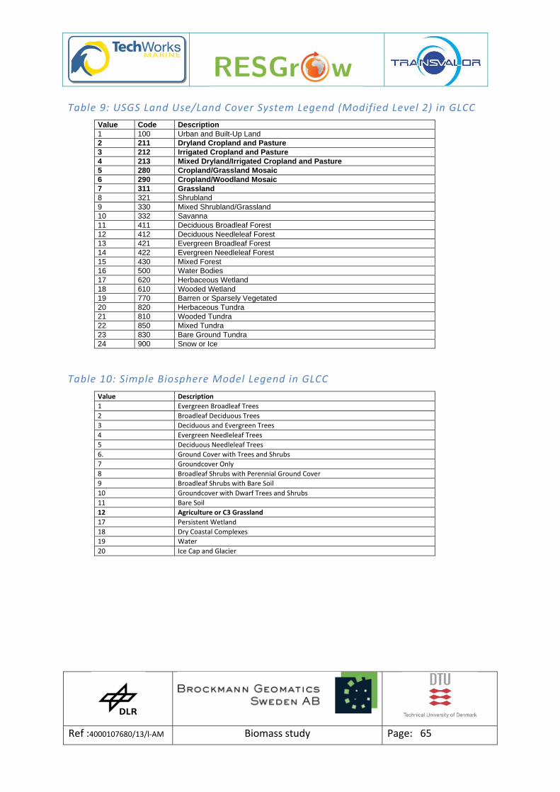
Ref :4000107680/13/l‐AM Biomass study Page: 65
Table 9: USGS Land Use/Land Cover System Legend (Modified Level 2) in GLCC
Value Code Description 1 100 Urban and Built-Up Land 2 211 Dryland Cropland and Pasture 3 212 Irrigated Cropland and Pasture 4 213 Mixed Dryland/Irrigated Cropland and Pasture 5 280 Cropland/Grassland Mosaic 6 290 Cropland/Woodland Mosaic 7 311 Grassland 8 321 Shrubland 9 330 Mixed Shrubland/Grassland 10 332 Savanna 11 411 Deciduous Broadleaf Forest 12 412 Deciduous Needleleaf Forest 13 421 Evergreen Broadleaf Forest 14 422 Evergreen Needleleaf Forest 15 430 Mixed Forest 16 500 Water Bodies 17 620 Herbaceous Wetland 18 610 Wooded Wetland 19 770 Barren or Sparsely Vegetated 20 820 Herbaceous Tundra 21 810 Wooded Tundra 22 850 Mixed Tundra 23 830 Bare Ground Tundra 24 900 Snow or Ice
Table 10: Simple Biosphere Model Legend in GLCC
Value Description
1 Evergreen Broadleaf Trees
2 Broadleaf Deciduous Trees
3 Deciduous and Evergreen Trees
4 Evergreen Needleleaf Trees
5 Deciduous Needleleaf Trees
6. Ground Cover with Trees and Shrubs
7 Groundcover Only
8 Broadleaf Shrubs with Perennial Ground Cover
9 Broadleaf Shrubs with Bare Soil
10 Groundcover with Dwarf Trees and Shrubs
11 Bare Soil
12 Agriculture or C3 Grassland
17 Persistent Wetland
18 Dry Coastal Complexes
19 Water
20 Ice Cap and Glacier

Ref :4000107680/13/l‐AM Biomass study Page: 66
Table 11: Simple Biosphere 2 Model Legend in GLCC
Value Description
1 Broadleaf Evergreen Trees
2 Broadleaf Deciduous Trees
3 Broadleaf and Needleleaf Trees (Mixed trees)
4 Needle leaf Evergreen Trees
5 Needle leaf Deciduous Trees
6 Short Vegetation/C4 Grassland (Grass with 10 ‐ 40% woody cover)
7 Shrubs with Bare Soil (Grass with <10% woody cover)
8 Dwarf Trees and Shrubs
9 Agriculture or C3 Grassland
10 Water, Wetlands, Ice/Snow
Table 12: Biosphere‐Atmosphere Transfer Scheme Legend in GLCC
Value Description
1 Crops, Mixed Farming
2 Short Grass
3 Evergreen Needleleaf Trees
4 Deciduous Needleleaf Tree
5 Deciduous Broadleaf Trees
6 Evergreen Broadleaf Trees
7 Tall Grass
8 Desert
9 Tundra
10 Irrigated Crops
11 Semidesert
12 Ice Caps and Glaciers
13 Bogs and Marshes
14 Inland Water
15 Ocean
16 Evergreen Shrubs
17 Deciduous Shrubs
18 Mixed Forest
19 Interrupted Forest
20 Water and Land Mixtures
8.2.2 University of Maryland (UMD) 1km Global Land Cover Nearly at the same time as the Global Land Cover Characterisation Project was started, the University of Maryland began to develop the UDM global land cover dataset. This product is also based on AVHRR data (starting from 1981to 1994). In the UMD project not only the NDVI composites are used for classification but also all 5 spectral bands of AVHRR. Minimum annual red reflectance, peak annual Normalized Difference Vegetation Index (NDVI), and minimum brightness temperature of channel three were among the most used metrics (Hansen et al., 2000). The UMD utilized a simplified IGBP legend with only 14 classes (Table 13).

Ref :4000107680/13/l‐AM Biomass study Page: 67
Table 13: UMD Land Cover codes
Value Land Cover Type 0 Water 1 Evergreen Needleleaf Forest 2 Evergreen Broadleaf Forest 3 Deciduous Needleleaf Forest 4 Deciduous Broadleaf Forest 5 Mixed Forest 6 Woodland 7 Wooded Grassland 8 Closed Shrubland 9 Open Shrubland
10 Grassland 11 Cropland 12 Bare Ground 13 Urban and Built
8.2.3 CORINE Land Cover Project In 1985, the CORINE (Coordination of information on the environment) programme of the Commission European was initiated. The idea was to to compile information on the state of the environment with regard to certain topics of whole Europe with an area of more than 2.3 million km2 in the 12 countries (as member of the European Community in 1986) from 62° N (The Faeroes) to 28° S (Canary Islands) and from 14' W (Canary Islands) to 29° E (Kastellorizon) investigated at a scale of 1:100 000 i.e. 1500 standard map sheets produced using 10 different projection systems. The area of the smallest mapping unit is defined as 25 hectares (500m x 500 m). For more technical details see Büttner et al. 2002. . The land cover nomenclature is defined in three major levels, combining in the first level five headings, in the second level 15 headings and in the third level 44 headings. A full list of the land cover categories is given in Table 14. Together with the work to find environmental indicators, it is necessary to find methods for a quick and cost‐effective updating of the CORINE Land Cover data base. For many purposes the data sets will be more useful if the classes increase from today's 44 in three levels. A fourth and fifth level with regional assumptions may be developed. This could be relevant for bioenergy resource assessment.

Ref :4000107680/13/l‐AM Biomass study Page: 68
Table 14: CORINE Legend
Level 1 Level 2 Level 3
1. Artificial 1.1. Urban fabric 1.1.1. Continuous urban fabric surfaces
1.1.2. Discontinuous urban fabric
1.2. Industrial, commercial and transport units 1.2.1. Industrial or commercial units
1.2.2. Road and rail networks and associated land
1.2.3. Port areas
1.2.4. Airports
1.3. Mine, dump 1.3.1. Mineral extraction sites and construction sites
1.3.2. Dump sites
1.3.3. Construction sites
1.4. Artificial non‐agricultural vegetated areas 1.4.1. Green urban areas
1.4.2. Sport and leisure facilities
2. Agricultural 2.1.Arable land 2.1.1. Non‐irrigated arable land areas
2.1.2. Permanently irrigated land
2.1.3. Rice fields
2.2. Permanent crops 2.2.1. Vineyards
2.2.2. Fruit trees and berry plantations
2.2.3. Olive groves
2.3. Pastures 2.3.1. Pastures
2.4. Heterogeneous agricultural areas 2.4.1. Annual crops associated with permanent crops
2.4.2. Complex cultivation
2.4.3. Land principally occupied by agriculture, with significant areas of natural vegetation
2.4.4. Agro‐forestry areas
3. Forests and semi‐natural areas
3.1. Forests 3.1.1. Broad‐leaved forest
3.1.2. Coniferous forest
3.1.3. Mixed forest
3.2. Shrub and/or herbaceous vegetation association 3.2.1. Natural grassland
3.2.2. Moors and heathland
3.2.3. Sclerophyllous vegetation
3.2.4. Transitional woodland shrub
3.3. Open spaces with little or no vegetation 3.3.1. Beaches, dunes, and sand plains
3.3.2. Bare rock
3.3.3. Sparsely vegetated areas
3.3.4. Burnt areas
3.3.5. Glaciers and perpetual snow
4. Wetlands 4.1. inland wetlands 4.1.1. Inland marshes
4.1.2. Peatbogs
4.2. Coastal wetlands 4.2.1. Salt marshes
4.2.2. Salines
4.2.3. Intertidal flats
5. Water bodies 5.1. Inland waters 5.1.1. Water courses
5.1.2. Water bodies
5.2. Marine waters 5.2.1. Coastal lagoons
5.2.2. Estuaries
5.2.3. Sea and ocean
In 2004 the CORINE 2000 update was available for EU member states as well as associated countries after signing a letter of agreement at the European Environmental Agency (EEA). In 2006 the CORINE was updated for 37 European States with the reference year 2006, which was finished in 2010. Here the minimal classification unit was 25 ha, while a land cover change was investigated if 5 ha and more are influenced. As for CORINE 2000 the
Ref :4000107680/13/l‐AM Biomass study Page: 69
legend will comprise in total 44 classes in three hierarchical layers. The last step for monitoring the European land cover was started in 2011 by the Global Monitoring for Environment and Security (GMES) initiative (now called European Copernicus programme) by setting up the GIO‐land service. This service has the focus on
- a land cover change product between 2006 and 2012, - a land cover product for 2012 and - five pan‐European high‐resolution layers on land cover characteristics as
artificial surfaces, forest areas (including forest crown cover density and forest type
composition), agricultural areas (permanent grasslands) with continuous degree of
intensity wetlands (according to RAMSAR definition and wetland indicator),
and water bodies.
GIO‐land builds on the pre‐cursor Copernicus‐related FP7 project geoland2, which addressed amongst other both the local component (i.e. the Urban Atlas) and the continental component. The minimum mapping unit for the continental component is 1 ha (validated).
8.2.4 GLC 2000 In the framework of the Global Land Cover 2000 (GLC 2000), a land‐cover map has been produced at a spatial resolution of 1km x 1km using data from four sensors on‐board four different Earth observing satellites. Most of these data were acquired on a daily basis by the VEGETATION sensor on‐board the SPOT‐4 satellite between 01 November 1999 and 31 December 2000. A description of GLC 2000 is given by Bartholomé et al. 2005, while the GLC 2000 legend is presented in Table 15.

Ref :4000107680/13/l‐AM Biomass study Page: 70
Table 15: GLC 2000 legend
GLC Global Class (according to LCCS terminology)
1 Tree Cover, broadleaved, evergreed
2 Tree Cover, broadleaved, deciduous, closed
3 Tree Cover, broadleaved, deciduous, open
4 Tree Cover, needle-leaved, evergreen
5 Tree Cover, needle-leaved, deciduous
6 Tree Cover, mixed leaf type
7 Tree Cover, regularly flooded, fresh water (& brackish)
8 Tree Cover, regularly flooded, saline water,
9 Mosaic: Tree cover / Other natural vegetation
10
Tree Cover, burnt
11
Shrub Cover, closed-open, evergreen
12
Shrub Cover, closed-open, deciduous
13
Herbaceous Cover, closed-open
14
Sparse Herbaceous or sparse Shrub Cover
15
Regularly flooded Shrub and/or Herbaceous Cover
16
Cultivated and managed areas
17
Mosaic: Cropland / Tree Cover / Other natural vegetation
18
Mosaic: Cropland / Shrub or Grass Cover
19
Bare Areas
20
Water Bodies
21
Snow and Ice
22
Artificial surfaces and associated areas
Ref :4000107680/13/l‐AM Biomass study Page: 71
8.2.5 MODIS LCC product The MODIS Land Cover Type product contains five classification schemes, which describe land cover properties derived from observations spanning a year’s input of Terra‐ and Aqua‐MODIS data. The primary land cover scheme identifies 17 land cover classes defined by the International Geosphere Biosphere Programme (IGBP), which includes 11 natural vegetation classes, 3 developed and mosaicked land classes, and three non‐vegetated land classes. The MODIS Terra and Aqua Land Cover Type Yearly L3 Global 500 m SIN Grid product incorporates five different land cover classification schemes, derived through a supervised decision‐tree classification method:
Land Cover Type 1: IGBP global vegetation classification scheme
Land Cover Type 2: University of Maryland (UMD) scheme
Land Cover Type 3: MODIS‐derived LAI/fPAR scheme
Land Cover Type 4: MODIS‐derived Net Primary Production (NPP) scheme
Land Cover Type 5: Plant Functional Type (PFT) scheme V051 Land Cover Type products are produced with revised training data and certain algorithm refinements. The Land Cover Dynamics product (MOD12Q2) provides estimates of the timing of vegetation phenology at global scales. The data layers included identify the timing of vegetation growth, maturity, and senescence that mark the seasonal cycles. The bi‐annual product uses 24 months of data as input, cantered on a 12‐month focus period of interest that is bracketed with six months of data on either end. Using this input, the land cover dynamics product provides estimates of vegetation phenology twice a year. The two 12‐month focus periods are July through June, and January through December, allowing for hemispheric differences in the growing seasons, and enabling the product to capture two growth cycles if necessary.
8.2.6 GLOBCOVER Within the ESA funded project GlobCover a global land cover map with 300 m resolution was developed. The map represents the land cover of 2005, especially the time from 1st December 2004 to 31st March 2006. The map is based on MERIS full resolution (FR) data (level 1B) in full swath width ranging from 86° N to 56° S depending on the season. The classification is performed in a spectro‐temporal procedure supported by the FAO Land Cover Classification System (FAO‐LCCS). It is designed to be compatible with the Global Land Cover map previously produced for the JRC for the year 2000, a one‐kilometre resolution

Ref :4000107680/13/l‐AM Biomass study Page: 72
map produced from SPOT‐4 Vegetation instrument data and known as GLC2000. It comprises 22 vegetation classes which are presented in Table 15. In 2010, the GlobCover chain was run by ESA and the Université Catholique de Louvain (UCL) in order to produce bimonthly and annual MERIS FR mosaics for the year 2009 and to derive a new global land cover map from this time series of MERIS FR 2009 mosaics.
Table 16: GlobCover classes
Value GlobCover legend
1 Post‐flooding or irrigated croplands
2 Rainfed croplands
3 Mosaic Cropland (50‐70%) / Vegetation (grassland, shrubland, forest) (20‐50%)
4 Mosaic Vegetation (grassland, shrubland, forest) (50‐70%) / Cropland (20‐50%)
5 Closed to open (>15%) broadleaved evergreen and/or semi‐deciduous forest (>5m)
6 Closed (>40%) broadleaved deciduous forest (>5m)
7 Open (15‐40%) broadleaved deciduous forest (>5m)
8 Closed (>40%) needleleaved evergreen forest (>5m)
9 Open (15‐40%) needleleaved deciduous or evergreen forest (>5m)
10 Closed to open (>15%) mixed broadleaved and needleleaved forest (>5m)
11 Mosaic Forest/Shrubland (50‐70%) / Grassland (20‐50%)
12 Mosaic Grassland (50‐70%) / Forest/Shrubland (20‐50%)
13 Closed to open (>15%) shrubland (<5m)
14 Closed to open (>15%) grassland
15 Sparse (>15%) vegetation (woody vegetation, shrubs, grassland)
16 Closed (>40%) broadleaved forest regularly flooded ‐ Fresh water
17 Closed (>40%) broadleaved semi‐deciduous and/or evergreen forest regularly flooded ‐ Saline water
18 Closed to open (>15%) vegetation (grassland, shrubland, woody vegetation) on regularly flooded or waterlogged soil ‐ Fresh, brackish or saline water
19 Artificial surfaces and associated areas (urban areas >50%)
20 Bare areas
21 Water bodies
22 Permanent snow and ice

Ref :4000107680/13/l‐AM Biomass study Page: 73
8.2.7 Future activities
8.2.7.1 Land Cover ECV As part of the ESA Climate Change Initiative (CCI), the Land_Cover_cci project is concerned with the generation of a global land cover map as one Essential Climate Variable (ECV) based on EO data. More particularly, the overall Land_Cover_cci objective is to critically revisit all algorithms required for the generation of a global land product in the light of GCOS requirements, and to design and demonstrate a prototype system delivering in a consistent way over years and from various EO instruments global land cover information matching the needs of key users’ belonging to the climate change community. In total three global maps will be produced for 2000, 2005 and 2010
8.3 Leaf Area Index
The Leaf Area Index (LAI) is the ratio of total upper leaf surface of a crop divided by the surface area of the land on which the crop grows. The LAI is a dimensionless number.
Forestry scientists define Leaf Area Index as the one‐sided green leaf area per unit ground area in broadleaf canopies. In conifers, three different definitions have been used:
Total needle surface area per unit ground area
Half of the total needle surface area per unit ground area
Projected needle area per unit ground area (source: http://en.wikipedia.org/wiki/Leaf_Area_Index)
8.3.1 LAI derived from the VEGETATION instrument In version 3 of the CYCLOPES algorithms LAI, Fraction of Cover (Fcover) and Fraction of Absorbed Photosynthetic Active Radiation (FAPAR) are assessed by inverting the radiative transfer model SAIL (Verhoef, 1984) using neural networks. First, the FAPAR is calculated using as network input the solar zenith angle at 10:00 local time and the normalized nadir reflectances in red, NIR and SWIR wavebands. In a second step, the LAI and Fcover are assessed by 2 different networks using the same input plus the FAPAR. This method, defined by the CSE team of Inra Avignon, is applied to VEGETATION data (Figure 18).
The CYCLOPES LAI participates in a validation exercise of existing global LAI products, coordinated by GSFC/NASA in collaboration with POSTEL and other product providers. The procedure consists of:
the intercomparison with LAI products derived in the frame of other projects (MODIS, GLOBCARBON, ECOCLIMAP, CCRS)

Ref :4000107680/13/l‐AM Biomass study Page: 74
the comparison with in‐situ measurements collected over the experimental site of ground networks (VALERI, BIGFOOT,...), and up‐scaled using high resolution satellite images.
First results, presented at the Global Land Monitoring Workshop, held in Missoula, from August 8th to 10th, 2006, show that the CYCLOPES LAI displays the best spatio‐temporal consistency, and fits best with the ground measurements, in spite of a low LAI level over the densest vegetation (source: http://smsc.cnes.fr/VEGETATION/lien1_appli.htm)
Figure 18: CYCLOPES 10‐day LAI derived from VEGETATION data (1km spatial resolution) for the period Julian day 182 of 2000.

Ref :4000107680/13/l‐AM Biomass study Page: 75
8.3.2 GEOLAND LAI The aim of the Geoland2 project is to constitute a step forward the implementation of the GMES Land Monitoring Core Service (LMCS). It is subdivided into three components: Local, Continental, and Global. The architecture of geoland2 is made of two different layers:
the Core mapping Services (CMS)
the Core Information services (CIS)
Bio‐geophysical Parameters (BioPar) CMS aims at setting‐up pre‐operational infrastructures for providing regional, European, and global bio‐geophysical variables, both in near real time and off‐line mode, to describe the continental vegetation state, the radiation budget at the surface, and the water cycle. The user‐driven service BioPar CMS aims at a portfolio to fulfil the needs of geoland‐2 CIS and CMS, which is considered as good proxies of a large community of users. The derivation of the product is based on the previous work of (Verger et al., 2008) demonstrating that neural networks could be trained to consistently estimate a given product from the reflectance measured by different sensors. Neural networks were trained to estimate LAI from SPOT VEGETATION daily time series of reflectance observations. Then, the resulting daily products are composited and gap filled to provide a smooth and continuous series of observations. The gap filling and smoothing is mainly based on the use of the climatology of daily products. Finally, the resulting smoothed and gap filled products based on climatology are fused with a product derived more closely to the daily observations. The customized 10‐day LAI products are currently available from 1999 onwards until today. A product example is presented in Figure 19.

Ref :4000107680/13/l‐AM Biomass study Page: 76
Figure 19: Geoland2 10‐day LAI composite derived from VEGETATION data (1 km spatial resolution) for the period 01.‐10.09.2012.
8.3.3 MODIS LAI The University of Boston, Department of Geography, delivers global LAI products based on Terra/Aqua‐MODIS Fraction of Absorbed Photosynthetic Active Radiation (FPAR) products (MOD15A2, MYD15A2). The FPAR products were re‐processed in January 2005 due to a bug in the original calculation of FPAR. FPAR under diffuse radiation was produced instead of FPAR under direct solar radiation, as required by the product specifications.
LAI is derived from FPAR products taking into account a six biome land cover classification which is based on the MODIS land cover product (MOD12). Each biome represents a pattern of the architecture of an individual tree (leaf normal orientation, stem‐trunk‐branch area fractions, leaf and crown size) and the entire canopy (trunk distribution, topography), as well as patterns of spectral reflectance and transmittance of vegetation elements. The soil and/or understory type are also characteristics of the biome, which can vary continuously within given biome‐dependent ranges. The distribution of leaves is described by the leaf area density distribution function which also depends on some continuous parameters. The six biomes are:

Ref :4000107680/13/l‐AM Biomass study Page: 77
grasses and cereal crops (biome 1)
shrub (biome 2)
broad leaf crops (biome 3)
savannah (biome 4)
broad leaf forest (biome 5)
needle forest (biome 6)
The following land cover classes are excluded from the calculation:
Urban, built‐up class
Permanent wetlands, marshes
Perennial snow, ice, tundra
Barren, desert, or very sparsely vegetated
Water (ocean or in land)
The level‐4 MODIS global Leaf Area Index (LAI) and Fraction of Photosynthetic Active Radiation (FPAR) product is composited every 8 days at 1‐kilometer resolution on a Sinusoidal grid. The product is available from February 2000 until now.
A summary of the available global LAI time series is shown in Table 17.
Table 17: Summary of available LAI products
Project Coverage Period Spat. resolution
Time resolution Sensor
UNI Boston Global 07/1981 – 05/2001 0.5° monthly AVHRR
UNI Boston Global 07 / 1981 – 05 / 2001 16 km monthly AVHRR
ISLSCP Global 1987 ‐ 1988 1° monthly AVHRR
Cyclopes Global 1999 ‐ 2007 1 km
10 day
VEGETATION
Geoland Global 1999 ‐ present 1 km VEGETATION
Polder
Global
1996 ‐ 1997 6km POLDER‐1
2003 POLDER‐2
AMMA
West Africa
1996 ‐ 1997 0.05°
10 day POLDER‐1
2003 POLDER‐2
2000 ‐ 2005 0.01° monthly MODIS
Atlantic
1981 ‐ 2001 0.25° monthly AVHRR
1996 ‐ 1997
0.05°
10 day POLDER‐1
2003 POLDER‐2

Ref :4000107680/13/l‐AM Biomass study Page: 78
ECOCLIMAP Global 1992 – 1993, 1997 1 km monthly AVHRR
GLOBCARBON Global 1998 ‐ 2007 1 km, 10 km,
0.25°, 0.5°
10 day ATSR, VEGETATION
MOD15A2 Global 2000 – present 1 km Daily and 8 day
MODIS Terra/Aqua
MOD15_BU / MYD15_BU
Global 2000 ‐ 2006 1 km, 4 km, 0.25°
monthly MODIS Terra/Aqua
MOD15_BU / MYD15_BU
Global 2000 ‐ 2006 0.25° 8 day MODIS Terra/Aqua
Land‐SAF Atlantic 2010 ‐ present 1 km 10 days and monthly
MSG SEVIRI
GLOBMAP Global 1981 – 2011 8 km Half monthly (1981 – 2000) and 8 day (2000
‐ 2011
MODIS Terra/Aqua and AVHRR
8.4 Net Primary Productivity
Net primary productivity (NPP) can be taken as a measure of carbon uptake and biomass growth for perennials which are completely harvested every year. The uptake of carbon starts at zero and growth is described directly by NPP. For forests and shrubs, this approach is not applicable, as trees have a much longer lifetime and the carbon uptake in different parts of the tree is a function of the tree’s age. Therefore, an initial biomass database describing both biomass amount and age of forests e.g. for the year 2000 as reference year is needed to calculate the annual growth on the basis of NPP. Radar data could be a source, but unfortunately saturation of the signal is reached at approx. 150 t/ha biomass which means that only boreal forests can be treated. Generally, there are only a few operational net primary productivity products available from remote sensing, but none of the products provides NPP separated for all relevant energy crops. The DLR approach using the BETHY/DLR model (Wißkirchen et al., 2013; Tum, 2012) provides NPP for C3 and C4 grass separately and for arable crops. Rice, maize, sugar beet, barley, wheat and sugar cane are treated separately and provide information on dedicated energy crops.

Ref :4000107680/13/l‐AM Biomass study Page: 79
The NASA MODIS NPP product is a 1 km global product provided once every 8 days. This product is currently in the experimental stage. The MYD17A2 algorithm uses input from MODIS LAI/FPAR (MYD15A2), land cover (MOD12), and biome‐specific climatology data from NASA's Data Assimilation Office (DAO). The MOD12 land cover product consists of the land cover classes broadleaf evergreen forest, coniferous evergreen forest, high latitude deciduous forest, tundra, mixed deciduous and evergreen forest, wooded grassland, grassland, bare ground, cultivated, broadleaf deciduous forest, shrubs and bare ground
8.5 Meteorological parameters
Besides solar radiation, meteorological parameters used for dynamic vegetation modelling are temperature and precipitation. They are typically obtained from meteorological numerical weather modelling as e.g. provided by ECMWF or NCEP meteorological centres. Satellite‐based data is widely used in numerical weather modelling as input data, but we don’t see a direct relationship of the use of EO data for this purpose.
8.6 Photosynthetic active radiation
Photosynthetic active radiation is defined as the photon flux density (photons per second per square meter) within the visible wavelength range (usually 400 to 700 nm). It indicates the total energy available to plants for photosynthesis, and is thus a key parameter for biological and ecological studies. PAR can be derived via a statistical approach from global radiation. For dynamic vegetation modelling daily values of global irradiation needs to be provided, for statistical approaches monthly or yearly sums are used.

Ref :4000107680/13/l‐AM Biomass study Page: 80
9 References
Bartholome, E., Belward, A. S., 2005: GLC2000: a new approach to global land cover mapping from Earth observation data. Int. J. Remote Sensing, 26 (9), 1959‐1977. doi:10.1080/01431160412331291297 Bergen, K.M., Dobson, M.C., 1999: Integration of remotely sensed radar imagery in modelling and mapping of forest biomass and net primary production. Ecological Modelling 122, 257–274. doi:10.1016/S0304‐3800(99)00141‐6 BMU, 2011a: Renewable Energies – Perspectives for a Sustainable Energy Future, Federal Ministry for the Environment, Nature Conservation and Nuclear Safety, Germany. http://www.erneuerbare‐energien.de/fileadmin/ee‐import/files/pdfs/allgemein/application/pdf/ee_innovationen_energiezukunft_en_bf.pdf BMU, 2011b: Renewable Energy Sources in Figures – National and International Development, Federal Ministry for the Environment, Nature Conservation and Nuclear Safety, Germany. http://www.erneuerbare‐energien.de/fileadmin/Daten_EE/Dokumente__PDFs_/ee_in_zahlen_en_bf.pdf BMU, 2006: Renewable Energies – Innovations for the Future, Federal Ministry for the Environment, Nature Conservation and Nuclear Safety, Germany. http://www.bmu.de/fileadmin/bmu‐import/files/pdfs/allgemein/application/pdf/ee_innovationen_energiezukunft_en_bf.pdf Büttner, G., Feranec, J., Jaffrain, G., 2002: Corine, Land Cover Update 2000. Technical guidelines. Technical Report 89, European Environment Agency. http://edz.bib.uni‐mannheim.de/daten/edz‐bn/eua/02/techrep89.pdf Cai, Z., Sawamoto, T., Li, C., Kang, G., Boonjawat, J., Mosier, A., et al., 2003: Field validation of the DNDC model for greenhouse gas emissions in East Asian cropping systems. Glob Biogeochem Cycles, 17(4), 1e10. doi:10.1029/2003GB002046 Collatz, G.J., Ribas‐Carbo, M., Berry, J.A., 1992: Coupled Photosynthesis – stomatal conductance model for leaves of C4 plants. Aust. J. Plant Physiol., 19, 519‐538. doi:10.1071/PP9920519 ESA, 2012: Report for Mission Selection: Biomass. ESA SP‐1324/1 (3 volume series), European Space Agency, Noordwijk, The Netherlands. http://esamultimedia.esa.int/docs/EarthObservation/SP1324‐1_BIOMASSr.pdf

Ref :4000107680/13/l‐AM Biomass study Page: 81
European Commission, 2009: Directive 2009/28/EC of the European parliament and of the council of 23 April 2009 on the promotion of the use of energy from renewable sources and amending and subsequently repealing Directives 2001/77/EC and 2003/30/EC. http://eur‐lex.europa.eu/LexUriServ/LexUriServ.do?uri=OJ:L:2009:140:0016:0062:EN:PDF European Commission, 2012: Europe in figures – Eurostat yearbook 2012. http://epp.eurostat.ec.europa.eu/cache/ITY_OFFPUB/KS‐CD‐12‐001/EN/KS‐CD‐12‐001‐EN.PDF Farquhar, G.D., von Caemmerer, S., Berry, J.A., 1980: A biochemical model of photosynthesis in leaves of C3 species. Planta, 149, 58‐90. doi:10.1007/BF00386231 Fatoyinbo, A., 2012: Remote Sensing of Biomass – Principles and Application. InTech. doi:10.5772/696. Fischer, G., van Velthuizen, H., Nachtergaele, F.O., 2000: Global Agro‐Ecological Zones Assessment: Methodology and Results. Interim Report IR‐00‐064, FAO (Food and Agriculture Organization of the United Nations), International Institute for Applied Systems Analysis (IIASA). http://www.iiasa.ac.at/publication/more_IR‐00‐064.php FNR (Fachagentur Nachwachsende Rohstoffe e.V.), 2007: Leitfaden Bioenergie – Planung, Betrieb und Wirtschaftlichkeit von Bioenergieanlagen, ISBN 3‐00‐015389‐6. http://fnr‐server.de/cms35/fileadmin/biz/pdf/leitfaden/leitfaden_bioenergie.pdf Hansen, M.C., DeFries, R.S., Townshend, J.R.G., Sohlberg, R., 2000: Global land cover classification at 1 km spatial resolution using a classification tree approach. Int. J. Remote Sensing, 21 (6/7), 1331‐1364. http://modis.gsfc.nasa.gov/sci_team/pubs/abstract.php?id=03529 Gonzales‐Alonso, F., Merion‐Demiguel, S., Roldan‐Zamarron, A., Garccia‐Gigorro, S., Cuevas, J. M., 2006: Forest biomass estimation through NDVI composites. The role of remotely sensed data to assess Spanish forests as carbon sinks. International Journal of Remote Sensing 27 (24), 5409–5415. doi:10.1080/01431160600830748 International Energy Agency (IEA), 2011: World Energy Outlook. http://www.worldenergyoutlook.org International Energy Agency (IEA), 2007: Bioenergy Project Development and Biomass Supply – Good Practise Guidelines. http://www.iea.org/publications/freepublications/publication/biomass.pdf

Ref :4000107680/13/l‐AM Biomass study Page: 82
IPCC, 2011: Edenhofer, O., Pichs‐Madruga, R.,, Sokona, Y., Seyboth, K., Matschoss, P., Kadner, S., Zwickel, T., Eickemeier, P., Hansen, G., Schloemer, S., von Stechow, C. (Eds.) Cambridge University Press, Cambridge, United Kingdom and New York, NY, USA, 1075 pp. Available from Cambridge University Press, The Edinburgh Building Shaftesbury Road, Cambridge CB2 2RU England. http://www.ipcc.ch/publications_and_data/publications_and_data_reports.shtml Jones, C.A., Kiniry, J.R., 1986: CERES‐Maize: a simulation model of maize growth and development. Texas A & M University Press. ISBN‐13: 978‐0890962695 Kindermann, G., Schörghuber, S., Linkosalo, T., Sanchez, A., Rammer, W., Seidl, R., Lexer, M., 2013: Potential stocks and increments of woody biomass in the European Union under different management and climate scenarios. Carbon Balance and Management, 8:2, http://www.cbmjournal.com/content/8/1/2 Knorr, W., Heimann, M., 2001: Uncertainties in global terrestrial biosphere modeling 1. A comprehensive sensitivity analysis with a new photosynthesis and energy balance scheme. Glob. Biogeochem. Cycles, 15, 207‐225. doi:10.1029/1998GB001059 Li, C., Frolking, S., Frolking, T.A., 1992: A model of nitrous oxide evolution from soil driven by rainfall events: 1. Model structure and sensitivity. J. Geophys. Res. ,97(D9): 9769e76. doi:1 0.1029/92JD00509 Lu, D., 2006: The potential and challenge of remote sensing‐based biomass estimation. International Journal of Remote Sensing, 27(7), 1297‐1328. doi:10.1080/01431160500486732 Mirschel, W., Pommerening, J., Wenkel, K.‐O., 1995: Pflanzenwachstumsmodelle für Winterroggen und Wintergerste (AGROSIM‐WR, AGROSIM‐WG). In: Wenkel, K.‐O.; Mirschel, W. [Hrsg]: Agroökosystemmodellierung ‐ Grundlage für die Abschätzung von Auswirkungen möglicher Landnutzungs‐ und Klimaänderungen.‐ ZALF‐Bericht 24: 88‐132. Monsi, S., Saeki, T., 1953: Über den Lichtfaktor in den Pflanzengesellschaften und seine Bedeutung für die Stoffproduktion. Jpn. J. Bot., 14, 22‐52. doi:10.1093/aob/mci052 Monteith, J.L., 1965: Evaporation and Environment in the State and Movement of Water in Living Organisms. Symposia of the Society for Experimental Biology, 19, 205‐234. http://www.unc.edu/courses/2007fall/geog/801/001/www/ET/Monteith65.pdf Monteith, J.L., 1977: Climate and the efficiency of crop production in Britain. Philosophical Transactions of the Royal Society, London B, 281, 277‐294. doi:10.1098/rstb.1977.0140

Ref :4000107680/13/l‐AM Biomass study Page: 83
Palosue, T., Kersebaum, K.C., Angulo, C., Hlavinka, P., Moriondo, M., Olesen, J.E., Patil, R.H., Ruget, F., Rumbaur, C., Takác, J., Trnka, M., Bindi, M., Caldag, B., Ewert, F., Ferrise, R., Mirschel, W., Saylan, L., Siska, B., Rötter, R., 2011: Simulation of winter wheat yield and its variability in different climates of Europe: A comparison of eight crop growth models. Europ. J. Agronomy, 35, 103– 114. doi:10.1016/j.eja.2011.05.001 Pflugmacher, D., 2007. Remote Sensing of Forest Aboveground Biomass using the Geoscience Laser Altimeter System. Master thesis, Oregon State University. REN21, 2013: Renewables Global Status Report. http://www.ren21.net/REN21Activities/GlobalStatusReport.aspx Seiler, R.A., Kogan, F., Sullivan, J., 1998: AVHRR‐based vegetation and temperature condition indices for drought detection in Argentina. Advances in Space Research 21, 481 – 484. doi:10.1016/S0273‐1177(97)00884‐3 Stange, F., Butterbach‐Bahl, K., Papen, H., Zechmeister‐Boltenstern, S., Li, C., Aber, J., 2000: A process‐oriented model of N2O and NO emissions from forest soils e 2. Sensitivity analysis and validation. J. Geophys. Res., 105(D4):4385e98. doi:10.1029/1999JD900948 Svoray, T., Shoshany, M., 2002: SAR‐based estimation of areal aboveground biomass (AAB) of herbaceous vegetation in the semi‐arid zone: a modification of the water‐cloud model. International Journal of Remote Sensing, 23, 4089–4100. doi:10.1080/01431160110115924 Tum, M., Buchhorn, M., Günther, K.P., Haller, B.C., 2011: Validation of modelled forest biomass in Germany using BETYH/DLR. Geosci. Model Dev., 4, 1019‐1034. doi:10.5194/gmd‐4‐1019‐2011 Tum, M., 2012: Modelling and validation of agricultural and forest biomass potentials for Germany and Austria. PhD Thesis, Göttingen. http://ediss.uni‐goettingen.de/handle/11858/00‐1735‐0000‐000D‐F07B‐A Tum, M., McCallum, I., Kindermann, G., Günther, K.P., Schmid, E. 2013: Sustainable Bioenergy Potentials for Europe and the Globe. Geoinfor Geostat: An Overview S1. doi:10.4172/2327‐4581.S1‐010 Verhoef, W., 1984: Light scattering by leaf layers with applications to canopy reflectance modelling: the SAIL model. Remote Sensing of Environment, 16,125‐141. doi:10.1016/0034‐4257(84)90057‐9

Ref :4000107680/13/l‐AM Biomass study Page: 84
Verger, A., Baret, F., Weiss, M., 2008: Performances of neural networks for deriving LAI estimates from existing CYCLOPES and MODIS products. Remote Sensing of Environment, 112(6), 2789‐2803. doi:10.1016/j.rse.2008.01.006 Wegehenkel, M., Brozio, S., Mirschel, W., Prietzsch, C., Zbell, B., 1999: Simulation Tool for the Evaluation of Agricultural Productivity (STEAP (Ertragspotential)). ProSmart‐Forschungs‐Endbericht (DLR‐Förderkennzeichen: 50EE9816), DaimlerChrysler Aerospace, Dornier Satellitensysteme, Dok.No.: EB‐DSS‐REP‐0001, 1999, S. 11/1 ‐ 11/62. Williams, J.R., 1995: The EPIC model. In: Singh, V.P. (Ed.): Computer Models of Watershed Hydrology. Water Resources Publications, Highlands Ranch, CO, 909‐1000. Wißkirchen, K., Tum, M., Günther, K.P., Niklaus, M., Eisfelder, C., Knorr, W., 2013: Quantifying the carbon uptake by vegetation for Europe on a 1 km² resolution using a remote sensing driven vegetation model. Geoscientific Model Development. 6, 1623‐1640. doi:10.5194/gmd‐6‐1623‐2013 Wißkirchen, K., 2005: Modellierung der regionalen CO2‐Aufnahme durch Vegetation. Dissertation an der Rheinischen Friedrich‐Wilhelms Universität Bonn, Mathematisch‐Naturwissenschaftliche Fakultät. Zheng, D., Rademacher, J., Chen, J., Crow, T., Bresee, M., Le MoineE, J., Ryu, S.‐R., 2004. Estimating aboveground biomass using Landsat 7 ETM+ data across a managed landscape in northern Wisconsin, USA. Remote Sensing of Environment 93, 402– 411. doi:10.1016/j.rse.2004.08.008