erm-ghana 09-051 final-2: 24 july 2009

ERM-Ghana 09-051 Final-2: 24 July 2009

Applied Science Associates

34

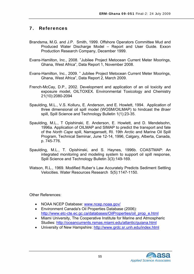
Figure 30. 48-hour spill of 1000 Tonnes crude at Well M1: model predicted water surface signature of the significant impacts spill.

Figure 31. 48-hour spill of 1000 Tonnes crude at Well M1: model predicted mass balance of the significant impacts spill.



35

Figure 32. 2-hour spill of 1000 Tonnes crude at the FPSO: model predicted water surface signature of the significant impacts spill.

Figure 33. 2-hour spill of 1000 Tonnes crude at the FPSO: model predicted mass balance of the significant impacts spill.



36

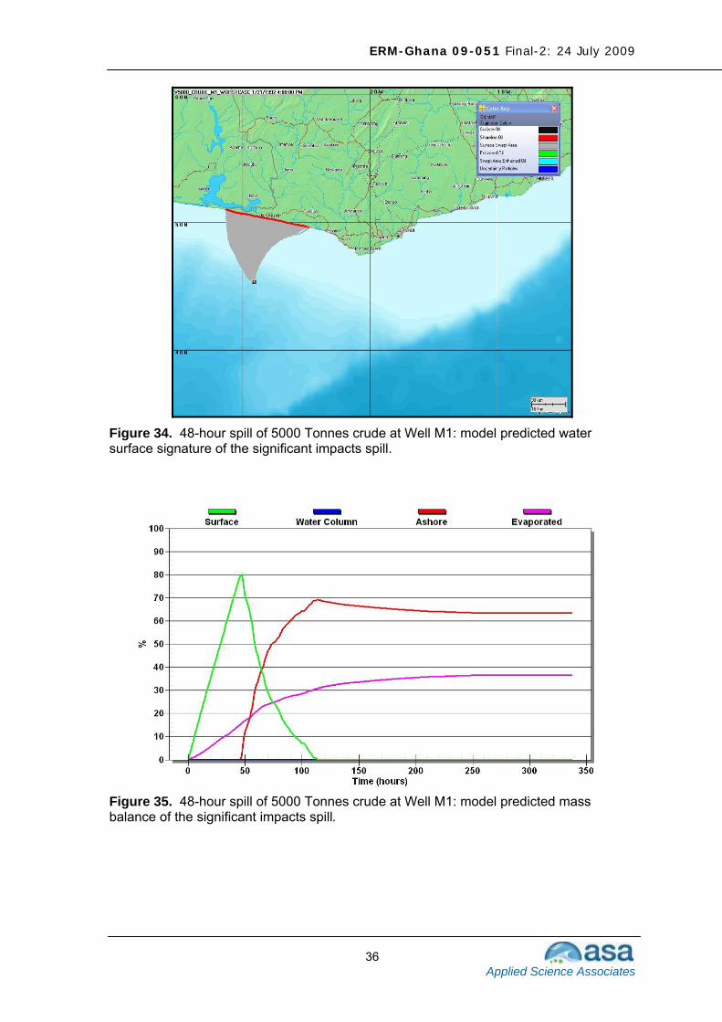
Figure 34. 48-hour spill of 5000 Tonnes crude at Well M1: model predicted water surface signature of the significant impacts spill.

Figure 35. 48-hour spill of 5000 Tonnes crude at Well M1: model predicted mass balance of the significant impacts spill.



37

Figure 36. 168-hour spill of 20,000 Tonnes crude at Well M1: model predicted water surface signature of the significant impacts spill.

Figure 37. 168-hour spill of 20,000 Tonnes crude at Well M1: model predicted mass balance of the significant impacts spill.



38

Figure 38. 48-hour spill of 28,000 Tonnes crude at Well M1: model predicted water surface signature of the significant impacts spill.

Figure 39. 48-hour spill of 28,000 Tonnes crude at Well M1: model predicted mass balance of the significant impacts spill.



39

Figure 40. 2-hour spill of 28,000 Tonnes crude at the FPSO: model predicted water surface signature of the significant impacts spill.

Figure 41. 2-hour spill of 28,000 Tonnes crude at the FPSO: model predicted mass balance of the significant impacts spill.



40

4. Produced Water Simulations Produced water discharges were simulated using ASA’s MUDMAP modeling system with ADCP current data input. Based on the operational production forecast (provided by the client), three discharge rates were chosen: 80, 18.4 and 6 Million Standard Barrels per Day (MSTB/D). These values represent the maximum the FPSO can process in a day, and maximum and average predicted discharges, respectively. Produced waters with a hydrocarbon concentration of 42 ppm are assumed to be discharged at the water surface at the FPSO. As previously described, the regional circulation is characterized by two periods: westward and eastward surface flows. These combinations lead to six simulations as defined in Table 5.

Table 5. Summary of produced water simulations

Simulation number

Discharge rate (MSTB/D)

Hydrocarbon concentration

(ppm) Flow

direction 1 80 42 westward 2 18.4 42 westward 3 6.0 42 westward 4 80 42 eastward 5 18.4 42 eastward 6 6.0 42 eastward

In each simulation, produced water is discharged continuously for 30 days, a period sufficiently long to capture variations of current speed and direction. Figures 44-49 show simulated 30 day average hydrocarbon distributions for the six scenarios listed in Table 5. Each figure shows both the horizontal and vertical extent of elevated hydrocarbon concentrations. Hydrocarbons rapidly disperse within a short distance and the vertical extent of the effluent is limited to less than 5 m for the predicted discharges and 7-8 m for the maximum possible discharge. In response to the westward currents, the hydrocarbon plume is transported to the northwest (Figures 42-44), whereas the eastward currents transport the plume to the east (Figures 45-47). The outermost concentration contour on the figures represents 0.005 ppm. This concentration represents a conservative estimate of the threshold for toxic effects to sensitive biota (French-McCay, 2002). The maximum distance from the discharge point to the 0.005 ppm contour is 2000-2200 m for the 80 MSTB/D discharge, 600-700 m for the 18.4 MSTB/D discharge, and 300-400 m for the 6.0 MSTB/D discharge. The results shown in Figures 42-47 assume a hydrocarbon concentration of 42 ppm in the produced water discharge. The contours scale linearly with the discharge hydrocarbon concentration. Thus if the produced water hydrocarbon concentration is 30 ppm, the contours are 71% of the values shown for 42 ppm; and for 20 ppm the contours are 48% of the values shown. For example, for a 30 ppm discharge, the 0.005 ppm contour shown in the figures represents 0.0036 ppm, the 0.01 ppm contour represents 0.007 ppm, the 0.02 ppm contour represents 0.014 ppm, et cetera. The area impacted by concentrations greater than 0.005 ppm is reduced for discharge concentrations of 30 or 20 ppm, but does not necessarily scale linearly with the 42 ppm discharge results.



41

Figure 42. Simulated hydrocarbon distribution with discharge conditions of 80 MSTB/D, 42 ppm, and westward flow.

Figure 43. Simulated hydrocarbon distribution with discharge conditions of 18.4 MSTB/D, 42 ppm, and westward flow.



42

Figure 44. Simulated hydrocarbon distribution with discharge conditions of 6.0 MSTB/D, 42 ppm, and westward flow.

Figure 45. Simulated hydrocarbon distribution with discharge conditions of 80 MSTB/D, 42 ppm, and eastward flow.



43

Figure 46. Simulated hydrocarbon distribution with discharge conditions of 18.4 MSTB/D, 42 ppm, and eastward flow.

Figure 47. Simulated hydrocarbon distribution with discharge conditions of 6.0 MSTB/D, 42 ppm, and eastward flow.



44

5. Drill Cuttings and Mud Discharge Simulations 5.1. Discharge Scenarios Drill cuttings and mud discharge simulations were conducted for Well M1, during both the westward- and eastward-directed current season. Water depth at the well site is 1193 m. The ADCP-observed current data described in Section 2.4 was used for the current input data in these dispersion simulations. A drilling program of up to four different sections was assumed. Error! Reference source not found.provides scenario specifications for the drill cuttings and mud modeling based on the expected drilling program provided by the client. The table lists the season, and the discharge amount, duration and location for each drilling section.

Table 6. Scenario specifications for the drill cutting scenarios

Season Section Diameter (inches)

Mud Discharged

(tonnes)

Cuttings Discharged

(tonnes) Start Date Duration

(hours) Discharge Location

1 36 7.3 115.2 2008-Oct-01 24 Seabed

2 26 185.7 456 2008-Oct-05 93.3 Seabed

3 17.5 8.8 352.8 2008-Oct-15 33.1 surface*

Westward Current Period

4 12.25 5.3 211.2 2008-Oct-21 90.2 surface*

1 36 7.3 115.2 2009-Jan-01 24 Seabed

2 26 185.7 456 2009-Jan-05 93.3 Seabed

3 17.5 8.8 352.8 2009-Jan-15 33.1 surface*

Eastward Current Period

4 12.25 5.3 211.2 2009-Jan-21 90.2 surface*

* Discharge: 15 m below the surface. The grain size distribution used in this study for the drill cuttings is adapted from Brandsma and Smith (1999), and is given in Table 7. The mud grain size distribution was adapted from Brandsma and Smith (1999), and is given in Table 8. The bulk density of the cuttings and mud are 2,400 kg/m3 and 1,198 kg/m3, respectively.

Table 7. Drill cuttings grain size distribution (adapted from Brandsma and Smith, 1999)

Particle Size (microns)

Percent Volume

Typical Settling Velocity (cm/s)

1 8 0.00014 3.5 6 0.00173

12.5 7 0.02233 41.1 3 0.23810 107.7 2 1.47659 217.2 18 4.07169 616.8 16 9.89828

1049.5 15 13.64825 3585.1 25 26.21170



45

Table 8. Mud grain size distribution for each drilling section (size distribution adapted from Brandsma and Smith, 1999)

Particle Size (microns)

Percent Volume

Typical Settling Velocity (cm/s)

3.7 1 0.0003 5.5 4 0.0006 8.6 19.2 0.0015 12.2 19.2 0.0031 14.8 13.3 0.0045 16 13.3 0.0053

17.9 10 0.0066 20.3 5 0.0085 46.5 8 0.0446 77.2 7 0.1222

5.2. Mud and Drilling Simulation Results Results of the mud and drill cuttings simulations are presented in terms of maximum predicted water column concentrations (Section 5.2.1) and predicted seabed deposition thickness (Section 5.2.2).

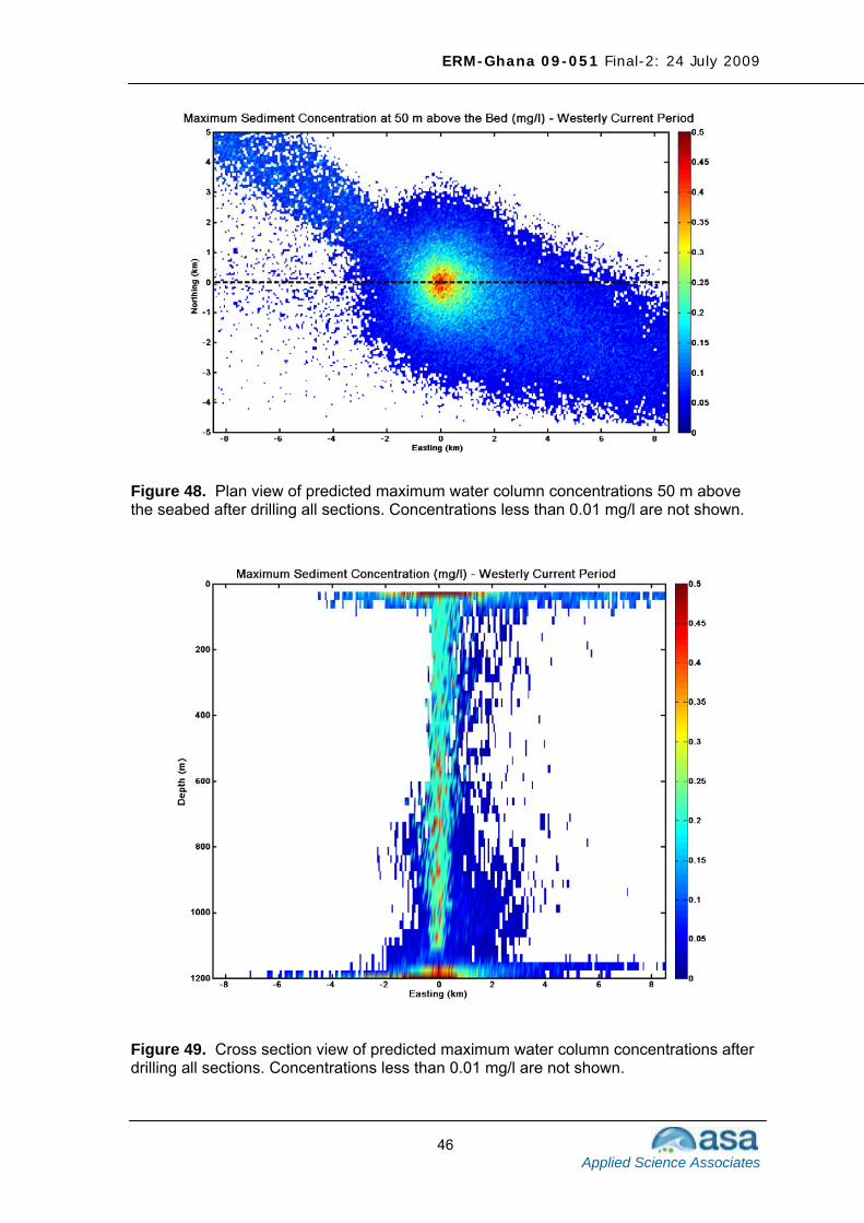
5.2.1. Predicted Water Column Concentration The water column concentrations of discharged material are a function of the discharge amount and ambient current strength/direction. Predicted water column concentrations were examined to determine maximum concentrations in the horizontal and vertical directions over the duration of the drilling period. The maximum concentrations are presented in Figures 48-51. The minimum water column concentration considered was 0.01 mg/l. This concentration is significantly below the threshold concentration for impacts to biota, but was selected to show the distribution of fine muds in the water column. The water column concentrations are primarily due to mud solids, since these particles have lower settling velocities and remain suspended in the water column for longer periods of time. In contrast, discharged cuttings settle to the seabed very quickly. Figures 48 and 49 show horizontal and vertical section views, respectively, of the maximum sediment concentrations during the westward current period. The main direction of suspended sediment dispersion is along a northwest-southeast axis following the flow pattern variation over the water column. The northwest plume is composed primarily of mud discharged at the surface during drilling sections 3 and 4, while the southeast plume contains the cuttings and muds discharged at the sea bed while drilling sections 1 and 2. The sediment plume with concentrations greater than 0.5 mg/l (the maximum concentration level shown in the figures) covers an area of approximately 0.015 km2 and does not extend more than 200 m from the well. Figures 50 and 51 show horizontal and vertical section views, respectively, of the maximum sediment concentrations for the eastward current period. As expected from the flow pattern, the sediment plume is primarily transported toward the east. The sediment plume with concentrations greater than 0.5 mg/l extends less than 100 m from the drilling position.



46

Figure 48. Plan view of predicted maximum water column concentrations 50 m above the seabed after drilling all sections. Concentrations less than 0.01 mg/l are not shown.

Figure 49. Cross section view of predicted maximum water column concentrations after drilling all sections. Concentrations less than 0.01 mg/l are not shown.



47

Figure 50. Plan view of predicted maximum water column concentration 50 m above the sea bed after drilling all sections. Concentrations less than 0.01 mg/l are not shown.

Figure 51. Cross section view of predicted maximum water column concentration after drilling all sections. Concentrations less than 0.01 mg/l are not shown.



48

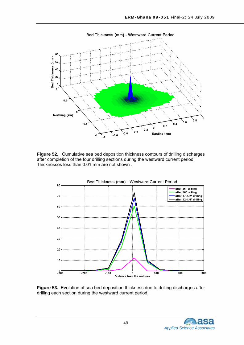
5.2.2. Predicted Seabed Deposition Thickness As a result of the particle settling velocities (Tables 7 and 8), cuttings settle relatively quickly compared to the discharged mud. Simulations were run under both westward and eastward current conditions; the results are similar for both. Table 9 presents the maximum predicted deposition thickness at any location at the end of drilling operations due to the discharge of cuttings and mud. This value represents the cumulative predicted deposition after all well sections have been drilled and the cuttings discharged. It occurs in the immediate vicinity of the well site. Table 9 also shows the percent of the discharged cuttings and mud deposited within the study area. Table 9. Maximum predicted deposition thickness of drill cuttings and mud and percent deposited after drilling all four sections

Season Maximum

Deposition Thickness (mm)

Percent Deposited

Westward currents 73.2 88.8

Eastward currents 78.9 89.1

Figures 52 and 53 present the predicted deposition of the cuttings and mud released from all well sections during the westward current period. The majority of the deposited material is concentrated around the release location. The deposition pattern is roughly uniform in all directions with a slight bias to the north and east. Deposition is greater than 0.1 mm over an area of approximately 0.353 km2 and greater than 1 mm over an area of approximately 0.053 km2 (Table 10). Figure 54 depicts the cumulative mass of cuttings and mud deposited over time (as a percent of the total), showing 88.8 percent deposited. Figures 55 and 56 present the predicted deposition of the cuttings and mud released from all well sections during the eastward current period. The majority of the deposited material is concentrated near the release location. The deposition pattern is skewed toward the north and east. Deposition is greater than 0.1 mm over an area of approximately 0.343 km2 and greater than 1 mm over an area of approximately 0.053 km2 (Table 10). Figure 57 depicts cumulative mass of cuttings and mud deposited over time (as a percent of the total), showing 89.1 percent deposited. Table 10. Areal extent of seabed deposition by thickness interval.

Thickness (mm) Area for Westward Current Period (km2)

Area for Eastward Current Period (km2)

≤ 0.1 1.0625 1.1000 0.1 - 1.0 0.3000 0.2900

1.0 - 10.0 0.0450 0.0475 ≥ 10.0 0.0075 0.0050



49

Figure 52. Cumulative sea bed deposition thickness contours of drilling discharges after completion of the four drilling sections during the westward current period. Thicknesses less than 0.01 mm are not shown .

Figure 53. Evolution of sea bed deposition thickness due to drilling discharges after drilling each section during the westward current period.



50

Figure 54. Percent total mass of bulk material deposited over time during the westward current period.



51

Figure 55. Cumulative sea bed deposition thickness contours of drilling discharges after completion of the four drilling sections during the eastward current period. Thicknesses less than 0.01 mm are not shown .

Figure 56. Evolution of sea bed deposition thickness due to drilling discharges after drilling each section during the eastward current period.



52

Figure 57. Percent total mass of bulk material deposited over time during the eastward current period.



53

6. Conclusions Oil Spill Simulations OILMAP’s stochastic model was applied to eleven potential surface spill scenarios using WANE wind and current data. For all scenarios the predominant transport of spilled oil is to the east. The footprint for the area of potential impact varies with spill size, with the maximum length of the footprint ranging from 40 km for a marine gasoil spill of 10 Tonnes to more than 600 km for crude oil spills of 1000 Tonnes or more. Spilled oil could reach the Ghana shoreline in a minimum of 1-1.25 days although the average time to reach shore is 2.5-4.5 days. Roughly 200-300 km of shoreline is at risk for oiling with the larger spill sizes having the potential for more shoreline impact. The shoreline with the highest probability of being oiled is the 100 km west of Cape Three Points. East of Cape Three Points a longer reach of shoreline could potentially be oiled, but the probability of oiling is generally less than 10 percent. The shoreline east of Cape Three Points has the highest probability of oiling due to a 168-hour release of 20,000 Tonnes of crude oil from Well M1. For this scenario some areas have up to a 15 percent probability of being oiled. The stochastic simulations use winds and currents generated by model hindcasts. Such data is valuable for providing long time series of environmental conditions and is accurate in a statistical sense. However model-generated data may not replicate the very short-term or anomalous behavior that is often seen in observations. Such anomalous conditions represent a very low probability of occurrence and may not be reflected in the oil spill results. A trajectory/fate simulation was done for each spill scenario with shoreline impacts using the same simulation start date for each. The simulation time was chosen to encompass a period with winds and currents that result in a greater transport of oil to the shore than most other time periods. For these scenarios, the first oil reached shore, north and slightly west of the spill site, 45 hours after the spill began. The extent of shoreline oiling was directly related to the duration of the oil release. An instantaneous or 2-hour duration spill resulted in a relatively short (10-12 km) length of shoreline impacted. Longer duration spills contribute to wider spreading of surface oil due variations in the wind and current directions. For the 48-hour release 75 km of shoreline were impacted, and for the 168-hour release 125 km were oiled. The mass balance indicated 20-30% of the crude oil and approximately 60% of the marine gasoil evaporated before the oil reached shore.

Produced Water Simulations Produced water discharges were simulated using ADCP current data as input to ASA’s MUDMAP modeling system. Westward and eastward flow conditions were considered for maximum possible, and maximum and average predicted discharge rates. Based on a continuous surface discharge for 30 days, elevated hydrocarbon concentrations were found to be confined within a short distance of the release location for the maximum and average predicted discharges. The



54

maximum distance from the discharge point to the 0.005 ppm contour is 2000-2200 m for the maximum possible discharge (80 MSTB/D), 600-700 m for the maximum predicted discharge rate (18.4 MSTB/D), and 300-400 m for the average predicted discharge rate (6 MSTB/D). The vertical extent of the effluent remains within 5 m of the surface for the predicted discharge rates, and within 7-8 m of the surface for the maximum possible discharge. Drilling Discharge Simulations For the westward and eastward-current periods, four drilling section discharges were simulated. Water column concentrations are primarily due to mud solids, while the accumulated seabed deposition is primarily due to cutting discharges. The majority of deposition occurs close to the discharge site due to the relatively low current velocity. During the westward current period, the maximum horizontal extent of the discharge plume with a concentration greater than 0.5 mg/l is approximately 0.015 km2 and extends less than 200 m from the well. The larger size particles of the cutting discharges are deposited in the immediate vicinity of the well site, slightly oriented towards the north and east. The maximum deposition thickness is 73 mm within 25 m of the drilling site; the area covered by deposits more than 1 mm thick is approximately 0.053 km2. During the eastward current period, the maximum horizontal extent of the discharge plume with a concentration greater than 0.5 mg/l extends approximately 100 m from the drilling position. The maximum deposition thickness is 79 mm within 25 m of the drilling site, indicating that the majority of the deposited material is concentrated below the release location. The area with deposition greater than 1 mm is predicted to be approximately 0.053 km2.



55

7. References Brandsma, M.G. and J.P. Smith, 1999. Offshore Operators Committee Mud and

Produced Water Discharge Model – Report and User Guide. Exxon Production Research Company, December 1999.

Evans-Hamilton, Inc., 2008. ”Jubilee Project Metocean Current Meter Moorings,

Ghana, West Africa”, Data Report 1, November 2008. Evans-Hamilton, Inc., 2009. ” Jubilee Project Metocean Current Meter Moorings,

Ghana, West Africa”, Data Report 2, March 2009. French-McCay, D.P., 2002. Development and application of an oil toxicity and

exposure model, OILTOXEX. Environmental Toxicology and Chemistry 21(10):2080-2094

Spaulding, M.L., V.S. Kolluru, E. Anderson, and E. Howlett, 1994. Application of

three dimensional oil spill model (WOSM/OILMAP) to hindcast the Braer spill, Spill Science and Technology Bulletin 1(1):23-35.

Spaulding, M.L., T Opishinski, E. Anderson, E. Howlett, and D. Mendelsohn,

1996a. Application of OILMAP and SIMAP to predict the transport and fate of the North Cape spill, Narragansett, RI. 19th Arctic and Marine Oil Spill Program, Technical Seminar, June 12-14, 1996, Calgary, Alberta, Canada, p. 745-776.

Spaulding, M.L., T. Opishinski, and S. Haynes, 1996b. COASTMAP: An

integrated monitoring and modeling system to support oil spill response, Spill Science and Technology Bulletin 3(3):149-169.

Watson, R.L., 1969. Modified Ruber’s Law Accurately Predicts Sediment Settling

Velocities. Water Resources Research 5(5):1147-1150. Other References:

• NOAA NCEP Database: www.ncep.noaa.gov/ • Environment Canada's Oil Properties Database (2006):

http://www.etc-cte.ec.gc.ca/databases/OilProperties/oil_prop_e.html • Miami University, The Cooperative Institute for Marine and Atmospheric

Studies: http://oceancurrents.rsmas.miami.edu/atlantic/guiana.html • University of New Hampshire: http://www.grdc.sr.unh.edu/index.html



A-1

Appendix A: MUDMAP Model Description MUDMAP is a personal computer-based model developed by ASA to predict the near and far field transport, dispersion, and bottom deposition of drill muds and cuttings and produced water (Spaulding et al; 1994; Spaulding, 1994). In MUDMAP, the equations governing conservation of mass, momentum, buoyancy, and solid particle flux are formulated using integral plume theory and then solved using a Runge Kutta numerical integration technique. The model includes three stages: convective descent/ascent, dynamic collapse and far field dispersion. It allows the transport and fate of the release to be modeled through all stages of its movement. The initial dilution and spreading of the plume release is predicted in the convective descent/ascent stage. The plume descends if the discharged material is more dense than the local water at the point of release and ascends if the density is lower than that of the receiving water. In the dynamic collapse stage, the dilution and dispersion of the discharge is predicted when the release impacts the surface, bottom, or becomes trapped by vertical density gradients in the water column. The far field stage predicts the transport and fate of the discharge caused by the ambient current and turbulence fields. MUDMAP is based on the theoretical approach initially developed by Koh and Chang (1973) and refined and extended by Brandsma and Sauer (1983) for the convective descent/ascent and dynamic collapse stages. The far field, passive diffusion stage is based on a particle based random walk model. This is the same random walk model used in ASA’s OILMAP spill modeling system (ASA, 1999). MUDMAP uses a color graphics-based user interface and provides an embedded geographic information system, environmental data management tools, and procedures to input data and to animate model output. The system can be readily applied to any location in the world. Application of MUDMAP to predict the transport and deposition of heavy and light drill fluids off Pt Conception, California and the near field plume dynamics of a laboratory experiment for a multi-component mud discharged into a uniform flowing, stratified water column are presented in Spaulding et al. (1994). King and McAllister (1997, 1998) present the application and extensive verification of the model for a produced water discharge on Australia’s northwest shelf. GEMS (1998) presents the application of the model to assess the dispersion and deposition of drilling cuttings released off the northwest coast of Australia. MUDMAP References APASA (2004). “ Modelling studies to assess the fate of sediments released during June

2004 reclaimer jetty dredging operation.” Asia-Pacific Applied Science Associates report to Oceanica Consulting Pty.

Brandsma, M.G. and T.C. Sauer, Jr., 1983. “The OOC model: prediction of short term fate of drilling mud in the ocean, Part I model description and Part II model results”. Proceedings of Workshop on An Evaluation of Effluent Dispersion and Fate Models for OCS Platforms, Santa Barbara, California.

Brandsma, M.G. & Smith, J.P., 1999. Offshore Operators Committee Mud and Produced Water Discharge Model - Report and User Guide. Exxon Production Research Company, December 1999.



A-2

Burns, K., Codi, S., Furnas. M., Heggie. D., Holdway, D., King, B., and McAllister, F, 1999. “Dispersion and Fate of Produced Formation Water Constituents in an Australian Northwest Shelf Shallow Water Ecosystem”. Marine Pollution Bulletin Vol. 38, No 7 pp 593 – 603.

GEMS - Global Environmental Modelling Services, 1998. Quantitative assessment of the dispersion and seabed depositions of drill cutting discharges from Lameroo-1 AC/P16, prepared for Woodside Offshore Petroleum, prepared by Global Environmental Modelling Services, Australia, June 16, 1998.

King, B. and F.A. McAllister ,1997. "Modeling the Dispersion of Produced Water Discharge in Australia, Volume I and II". Australian Institute of Marine Science report to the APPEA and ERDC.

King, B. and F.A. McAllister ,1998. Modelling the dispersion of produced water discharges. APPEA Journal 1998, pp. 681-691.

Koh, R.C.Y. and Y.C. Chang, 1973. “Mathematical model for barged ocean disposal of waste”. Environmental Protection Technology Series EPA 660/2-73-029, U.S. Army Engineer Waterways Experiment Station, Vicksburg, Mississippi.

Khondaker, A. N., 2000. “Modeling the fate of drilling waste in marine environment – an overview”. Journal of Computers and Geosciences Vol 26, pp 531-540.

Nedweed, T, 2004. “ Best practices for drill cuttings and mud discharge modelling.” SPE 86699. Paper presented at the Seventh SPE International Conference on Health, Safety and Environment in Oil and Gas Exploration and Production, Calgary, Alberta, Canada. Society of Petroleum Engineers, P6.

Neff, J, 2005. “Composition, environment fates, and biological effect of water based drilling muds and cuttings discharged to the marine environment: A synthesis and annotated bibliography.” Report prepared for Petroleum Environment Research Forum and American Petroleum Institute.

Gallo. A and A. Rocha, 2006. “Computational modelling of drill cuttings and mud released in the sea from E&P activities in Brazil.” 9th International Marine Environmental Modelling Seminar.

Spaulding, M. L., T. Isaji, and E. Howlett, 1994. MUDMAP: A model to predict the transport and dispersion of drill muds and production water, Applied Science Associates, Inc, Narragansett, RI.



B-1

Appendix B: OILMAP Modeling System Description OILMAP is a state-of-the-art, personal computer based oil spill response system applicable to oil spill contingency planning and real time response and applicable for any location in the world (Jayko and Howlett, 1992; Spaulding et al., 1992a,b). OILMAP was designed in a modular fashion so that different types of spill models could be incorporated within the basic system, as well as a suite of sophisticated environmental data management tools, without increasing the complexity of the user interface. The model system employs a Windows based graphics user interface that extensively utilizes point and click and pull down menu operation. OILMAP is configured for operation on standard Pentium PCs and can be run on laptop and notebook computers to facilitate use in the field. The OILMAP suite includes the following models: a trajectory and fates model for surface and subsurface oil, an oil spill response model, and stochastic and receptor models. The relevant models are described in more detail below. The trajectory and fates model predicts the transport and weathering of oil from instantaneous or continuous spills. Predictions show the location and concentration of the surface and subsurface oil versus time. The model estimates the temporal variation of the oil’s areal coverage, oil thickness, and oil viscosity. The model also predicts the oil mass balance or the amount of oil on the free surface, in the water column, evaporated, on the shore, and outside the study domain versus time. The fate processes in the model include spreading, evaporation, entrainment or natural dispersion, and emulsification. As an option OILMAP can also estimate oil-sediment interaction and associated oil sedimentation. A brief description of each process algorithm is presented here. ASA (1999) provides a more detailed description for the interested reader. The oil sedimentation algorithm is described in French et al. (1994), ASA (1999) and Kirstein et al. (1985). Spreading is represented using the thick slick portion of Mackay et al.’s (1980, 1982) thick-thin approach. Evaporation is based on Mackay’s analytic formulation parameterized in terms of evaporative exposure (Mackay et al., 1980, 1982). Entrainment or natural dispersion is modeled using Delvigne and Sweeney’s (1988) formulation which explicitly represents oil injection rates into the water column by droplet size. The entrainment coefficient, as a function of oil viscosity, is based on Delvigne and Hulsen (1994). Emulsification of the oil, as function of evaporative losses and changes in water content, is based on Mackay et al. (1980, 1982). Oil-shoreline interaction is modeled based on a simplified version of Reed et al. (1989) which formulates the problem in terms of a shore type dependent holding capacity and exponential removal rate. For the subsurface component, oil mass injection rates from the surface slick into the water column are performed by oil droplet size class using Delvigne and Sweeney’s (1988) entrainment formulation. The subsurface oil concentration field is predicted using a particle based, random walk technique and includes oil droplet rise velocities by size class. The vertical and horizontal dispersion coefficients are specified by the user. Resurfacing of oil droplets due to buoyant effects is explicitly included and generates new surface slicks. If oil is resurfaced in the vicinity of surface spillets the oil is incorporated into the closest surface spillet. A more detailed presentation of the subsurface oil transport and fate algorithm is given in Kolluru et al. (1994). The basic configuration of the model also includes a variety of graphically based tools that allow the user to specify the spill scenario, animate spill trajectories, currents and winds, import and export environmental data, grid any area within the model operational domain, generate mean and/or tidal current fields, enter and edit oil types in the oil



B-2

library, enter and display data into the embedded geographic information system (GIS) and determine resources impacted by the spill. The GIS allows the user to enter, manipulate, and display point, line, poly line, and polygon data geographically referenced to the spill domain. Each object can be assigned attribute data in the form of text descriptions, numeric fields or external link files. In the stochastic mode spill simulations are performed stochastically varying the environmental data used to transport the oil. Either winds, currents, or both may be stochastically varied. The multiple trajectories are then used to produce contour maps showing the probability of surface and shoreline oiling. The trajectories are also analyzed to give travel time contours for the spill. These oiling probabilities and travel time contours can be determined for user selected spill durations. If resource information is stored in the GIS database a resource hit calculation can be performed to predict the probability of oiling important resources. OILMAP has been applied to hindcast a variety of spills. These hindcasts validate the performance of the model. Hindcasts of the Amoco Cadiz, Ixtoc and Persian Gulf War spills and an experimental spill in the North Sea by Warren Springs Laboratory are reported in Kolluru et al. (1994). Spaulding et al. (1993) also present a hindcast of the Gulf War spill. Spaulding et al. (1994) present the application of the model to the Braer spill where subsurface transport of the oil was critical to understanding the oil’s movement and impact on the seabed. Spaulding et al. (1996a) describes how the model had been applied to hindcast the surface and subsurface transport and fate of the fuel oil spilled from the North Cape barge. Integration of OILMAP with a real time hydrodynamic model and the hindcast of the movement of oil tracking buoys in Narragansett Bay are presented in Spaulding et al (1996b). OILMAP References Applied Science Associates, Inc. (ASA), 1999. OILMAP Technical and Users Manual

Applied Science Associates, Inc., Narragansett, RI.

Delvigne, G.A.L., and C.E. Sweeney. 1988. Natural dispersion of oil, Oil and Chemical Pollution 4:281-310.

Delvigne, G.A.L., and L.J.M. Hulsen, 1994. Simplified laboratory measurement of oil dispersion coefficient – Application in computations of natural oil dispersion. Proceedings of the Seventeenth Arctic and Marine Oil Spill Program, Technical Seminar, June 8-10, 1994, Vancouver, British Columbia, Canada, pp. 173-187.

French, D., E. Howlett, and D. Mendelsohn, 1994. Oil and chemical impact model system description and application, 17th Arctic and Marine Oil Spill Program, Technical Seminar, June 8-10, 1994, Vancouver, British Columbia, Canada, pp. 767-784.

Jayko, K. and E. Howlett, 1992. OILMAP an interactive oil spill model, OCEANS 92, October 22-26, 1992, Newport, RI.

Kirstein, B., J.R. Clayton, C. Clary, J.R. Payne, D. McNabb, G. Fauna, and R. Redding, 1985. Integration of suspended particulate matter and oil transportation study, Mineral Management Service, Anchorage, Alaska.

Kolluru, V., M.L. Spaulding, and E. Anderson, 1994. A three dimensional subsurface oil dispersion model using a particle based technique, 17th Arctic and Marine Oil



B-3

Spill Program, Technical Seminar, June 8-10, 1994, Vancouver, British Columbia, Canada, pp. 767-784.

Mackay, D., S. Paterson, and K. Trudel, 1980. A mathematical model of oil spill behavior, Department of Chemical Engineering, University of Toronto, Canada, 39 pp.

Mackay, D., W. Shui, K. Houssain, W. Stiver, D. McCurdy, and S. Paterson, 1982. Development and calibration of an oil spill behavior model, Report No. CG-D027-83, US Coast Guard Research and Development Center, Groton, CT.

Reed, M., E. Gundlach, and T. Kana, 1989. A coastal zone oil spill model: development and sensitivity studies, Oil and Chemical Pollution 5:411-449.

Spaulding, M. L., E. Howlett, E. Anderson, and K. Jayko, 1992a. OILMAP a global approach to spill modeling. 15th Arctic and Marine Oil Spill Program, Technical Seminar, June 9-11, 1992, Edmonton, Alberta, Canada, pp. 15-21.

Spaulding M. L., E. Howlett, E. Anderson, and K. Jayko, 1992b. Oil spill software with a shell approach. Sea Technology, April 1992. pp. 33-40.

Spaulding, M.L., E.L. Anderson, T. Isaji and E. Howlett, 1993. Simulation of the oil trajectory and fate in the Arabian Gulf from the Mina Al Ahmadi Spill, Marine Environmental Research 36(2):79-115.

Spaulding, M. L., V. S. Kolluru, E. Anderson, and E, Howlett, 1994. Application of three dimensional oil spill model (WOSM/OILMAP) to hindcast the Braer spill, Spill Science and Technology Bulletin 1(1):23-35.

Spaulding, M.L., T. Opishinski, E. Anderson, E. Howlett, and D. Mendelsohn, 1996a. Application of OILMAP and SIMAP to predict the transport and fate of the North Cape spill, Narragansett, RI. 19th Arctic and Marine Oil Spill Program, Technical Seminar, June 12-14, 1996, Calgary, Alberta, Canada, pp. 745-776.

Spaulding, M.L., T. Opishinski, and S. Haynes, 1996b. COASTMAP: An integrated monitoring and modeling system to support oil spill response, Spill Science and Technology Bulletin 3(3):149-169.



C-1

Appendix C: Selected Spill Scenarios

Typical, Representative Production Phase Oil Spill Scenarios Representative Oil Spill Size Drilling Scenarios Subsea Scenarios Production/ Topsides Scenarios Offloading/ Transfer Scenarios

ASA Oil Spill Modeling Scenario

Production Blowout (Small, Medium, Isolated) Well Release Production Blowout (Large, Isolated)

Release From Transfer Hose (Small) 1 (Crude from M1)

Manifold Release (Small, Medium Isolated) Drains Release

Manifold Release (Large, Isolated)

Riser Release(Small, Medium Isolated)

10 te (~73 bbls)

Well Test Release (Small) Riser Release Large Isolated)

Turret Leak (Small) Diesel/Marine Fuel Oil Transfer Release (Small, Medium) Vessel release (small) from collision

2 (Diesel from FPSO)

Diesel/Marine Fuel Oil Transfer Release (Large) Turret Leak (Medium)

Release From Transfer Hose (Medium) Vessel/FPSO release (medium) from collision

3 (Crude from MI) 3A (Crude from FPSO) 100 te

(~730 bbls) Reservoir Blowout (short duration)

Liquid Carry Over From Flare Diesel/Marine Fuel Oil Transfer Release (Large)

4 (Diesel from FPSO)

Turret Leak (Large) 1000 te (~7300 bbls)

Reservoir Blowout (48 hrs)

Crude Oil Tank Explosion

Transfer Hose Rupture (Isolated) Vessel/FPSO release (large) from collision

5 (Crude from MI) 5A (Crude from FPSO)

Production Blowout (Small, Unisolated) Manifold Release (Small, Unisolated)

5000 te (~37,000 bbls)

Reservoir Blowout (48 hrs) Riser Release (Small, Unisolated)

Turret Explosion (Escalated) 6 (Crude from MI)

Reservoir Blowout (> 5 days) Production Blowout (Medium, Large, Crude Oil Tank Explosion (Escalated)

Turret Leak (Escalated) 20,000 te (~146,000 bbls

Well Test Release (Un-isolated)

Manifold Release (Medium, Large, Unisolated) Escalated FPSO Loss Events

Transfer Hose Rupture (Unisolated) FPSO release (very large) from collision

7 (Crude from MI)

~28,000 te (~210,000 bbls) Riser Release (Medium, Large, Unisolated)

8 (Crude from MI) 8A (Crude from FPSO)

erm-ghana 09-051 final-2: 24 july 2009

Documents