erdc/itl tr-12-3 'simplified analysis procedures for
TRANSCRIPT
ERD
C/IT
L TR
-12
-3
Navigation Systems Research Program
Simplified Analysis Procedures for Flexible Approach Wall Systems Founded on Groups of Piles and Subjected to Barge Train Impact
Info
rmat
ion
Tec
hn
olog
y La
bor
ator
y
Robert M. Ebeling, Ralph W. Strom, Barry C. White, and Kevin Abraham
September 2012
Approved for public release; distribution is unlimited.

Navigation Systems Research Program ERDC/ITL TR-12-3 September 2012
Simplified Analysis Procedures For Flexible Approach Wall Systems Founded on Groups of Piles And Subjected To Barge Train Impact
Robert M. Ebeling, Barry C. White, and Kevin Abraham
Information Technology Laboratory U.S. Army Engineer Research and Development Center 3909 Halls Ferry Road Vicksburg, MS 39180-6199
Ralph W. Strom
9474 S.E. Carnaby Way Happy Valley, OR 97086
Final report
Approved for public release; distribution is unlimited.
Prepared for U.S. Army Corps of Engineers Washington, DC 20314-1000
Under Work Unit 88L1G1

ERDC/ITL TR-12-3 ii
Abstract
One type of flexible substructure used for new flexible approach wall structural system designs in the Corps is flexible pile groups. Simplified analysis procedures for flexible approach wall systems founded on groups of piles and subjected to barge train impact is discussed in this report. Pile bent groups of vertical piling and batter piling are investigated.
A “balance of energy” design procedure is presented. This procedure assumes that all the kinetic energy (KE) of the approaching barge train (normal to the wall) is converted to potential energy (PE), or strain energy, through deformation of the flexible piling. A pushover analysis technique is used to establish the potential energy (PE) capacity and displacement capacity of individual pile groups accounting for the various pile failure mechanisms. The total stored energy (PE) of the approach wall system will be the sum of the stored energy of all the pile groups reacting to the barge impact.
With three-dimensional (3-D) structural detailing of the impact deck (or beam), a model can be created where barge train impact loading may be shared by nearby supporting pile bents. The performance of this type of flexible approach wall system is also investigated.
DISCLAIMER: The contents of this report are not to be used for advertising, publication, or promotional purposes. Citation of trade names does not constitute an official endorsement or approval of the use of such commercial products. All product names and trademarks cited are the property of their respective owners. The findings of this report are not to be construed as an official Department of the Army position unless so designated by other authorized documents. DESTROY THIS REPORT WHEN NO LONGER NEEDED. DO NOT RETURN IT TO THE ORIGINATOR.

ERDC/ITL TR-12-3 iii
Contents Abstract ................................................................................................................................................... ii
Figures and Tables ................................................................................................................................. vi
Preface ..................................................................................................................................................... x
Unit Conversion Factors ...................................................................................................................... xii
1 Background and Proposed Engineering Procedures for the Simplified Analysis of Pile-Founded Flexible Approach Walls ........................................................................................ 1
1.1 Introduction .................................................................................................................. 1 1.2 Impact wall systems .................................................................................................... 6 1.3 Overview ....................................................................................................................... 7 1.4 Kinetic energy (KE) ...................................................................................................... 8 1.5 Barge impact velocities ............................................................................................... 9 1.6 Barge impact angle .................................................................................................... 11 1.7 Barge train size .......................................................................................................... 11 1.8 Hydrodynamic added mass ....................................................................................... 12 1.9 Load factors ............................................................................................................... 12 1.10 Potential energy (PE) and displacement capacity .................................................... 12 1.11 Performance objectives ............................................................................................. 13
1.11.1 Serviceability performance ..................................................................................... 13
1.11.2 Damage control performance ................................................................................ 13
1.11.3 Collapse prevention performance .......................................................................... 14 1.12 Load sharing .............................................................................................................. 14 1.13 Pushover analysis and force-deflection response ................................................... 15
1.13.1 Origin of pushover analysis in earthquake engineering ........................................ 17
1.13.2 Incremental analysis technique for barge impact loading in a pushover analysis ............................................................................................................................... 19
1.14 Non-linear conservation of energy ............................................................................ 21 1.15 Report contents ......................................................................................................... 22
2 Analytical Models For Drilled-In Place And Batter Piles .......................................................... 25
2.1 Introduction ................................................................................................................ 25 2.2 Drilled-in-pile (DIP) bent systems .............................................................................. 25
2.2.1 Point of fixity (POF) models .......................................................................................... 27
2.2.2 Analytical models suitable for pushover analyses ..................................................... 28
2.2.3 Capacity ........................................................................................................................ 28
2.2.4 Displacement limit state .............................................................................................. 29
2.2.5 Effective stiffness ......................................................................................................... 29 2.3 BP bent systems ........................................................................................................ 31
2.3.1 Analytical models ......................................................................................................... 32
2.3.2 Axial and flexural capacity ........................................................................................... 33

ERDC/ITL TR-12-3 iv
2.3.3 Pile axial and flexural interaction capacity effects ..................................................... 33 2.4 Simple interaction diagrams for piles ....................................................................... 33 2.5 Buckling effects on pile capacity .............................................................................. 36 2.6 Flexural hinge rotational capacity of piles ................................................................ 37 2.7 Cap beams ................................................................................................................. 39
3 Pushover Analysis of Drilled-In-Pile Bent Systems ................................................................... 41
3.1 Introduction ................................................................................................................ 41 3.2 Formulation of a pushover example problem .......................................................... 41 3.3 Determination of minimum embedment depth ....................................................... 43
3.3.1 Long pile behavior ........................................................................................................ 43
3.3.2 Depth of embedment by second zero deflection – p-y models ................................. 48
3.3.3 Depth of embedment by maximum negative deflection – p-y models ...................... 51
3.3.4 Depth of embedment by iteration – p-y models ......................................................... 52
3.3.5 Other observations regarding the design length and partial fixity ............................ 53
3.4 Equivalent depth to fixity for analytical models ....................................................... 56 3.4.1 Davisson (1970) equivalent free standing pile .......................................................... 56
3.4.2 Budeket al. (2000) analytical model ........................................................................... 56
3.4.3 Yang (1966) equivalent free standing pile ................................................................. 59 3.5 Effective stiffness – drilled in place piles ................................................................. 60 3.6 Pushover analysis of drilled-in-pile bents ................................................................. 61 3.7 DIP bent system ......................................................................................................... 62
3.7.1 Pushover analysis using Yang (1966) approach ........................................................ 63
3.7.2 Pushover analysis using Saul (1968) approach......................................................... 67
3.8 Results from pushover analysis ................................................................................ 69 3.9 Pile interaction effects ............................................................................................... 72 3.10 Summary and conclusions ........................................................................................ 74 3.11 Recommendations for further research ................................................................... 75
4 Pushover Analysis of Batter Pile Bent Systems ........................................................................ 76
4.1 Pushover analysis approach ..................................................................................... 76 4.2 Pushover analysis summary ..................................................................................... 80 4.3 Batter pile system kinetic energy absorption efficiency .......................................... 83 4.4 Practical consideration for pile batter ...................................................................... 88
5 Distribution of Barge Impact Loads to Adjacent Bents ........................................................... 90
5.1 Introduction ................................................................................................................ 90 5.2 Analytical approach ................................................................................................... 90 5.3 Maxwell’s Theorem .................................................................................................... 95
6 Conclusions and Future Research ............................................................................................. 97
6.1 Introduction ................................................................................................................ 97 6.2 Conclusions ................................................................................................................ 98 6.3 Future research .......................................................................................................... 99
6.3.1 Background .................................................................................................................. 99
6.3.2 Extending the research .............................................................................................. 102

ERDC/ITL TR-12-3 v
References ......................................................................................................................................... 108
Appendix A: Pushover analysis of drilled-in caisson, Fixed-head system Using Yang (1966), Saul (1968) and nonlinear p-y curve analysis........................................................... 113
Appendix B: Pushover analysis for batter-pile bent system ......................................................... 140
Appendix C: GROUP 7 Pushover analysis for batter-pile bent system ......................................... 170
Appendix D: Skin friction and tip capacities of piles ..................................................................... 177
Appendix E: Dynamic Response of Impact Wall Systems ............................................................ 192
Report Documentation Page

ERDC/ITL TR-12-3 vi
Figures and Tables
Figures
Figure 1-1. Conservation of energy for the barge train/flexible wall impact. ....................................... 2
Figure 1-2. Balance of energy approach. ................................................................................................. 3
Figure 1-3a. Impulse momentum approach. ........................................................................................... 4
Figure 1-3b. Steps in the impulse momentum analysis. ........................................................................ 5
Figure 1-3c. Pulse loading. ........................................................................................................................ 5
Figure 1-4. Barge train and velocity vector transformation – from local barge train to global (wall) axis (Arroyo-Caraballo and Ebeling (2006). ...................................................................... 10
Figure 1-5a. Load versus displacement plot for fixed-head bent - Serviceability performance of the usual load case. .................................................................................................... 15
Figure 1-5b. Load versus displacement plot for fixed-head bent - Damage control performance of the unusual load case. ................................................................................................. 16
Figure 1-5c. Load versus displacement plot for fixed-head bent - Collapse prevention performance of the extreme load case. ................................................................................................. 17
Figure 1-6a. Load versus displacement plot for BP bent - Serviceability performance. ................... 18
Figure 1-6b. Load versus displacement plot for pipe pile system - Damage control performance. ............................................................................................................................................ 18
Figure 1-6c. Load versus displacement plot for pipe pile system - Collapse prevention performance. ............................................................................................................................................ 19
Figure 1-7. Analysis of 3-D effects due to sharing of the impact load among pile groups. ............... 20
Figure 1-8. Load-displacement plot for fixed-head bent....................................................................... 22
Figure 2-1. DIP bent system. ................................................................................................................... 26
Figure 2-2. BP bent. ................................................................................................................................. 31
Figure 2-3. Pile axial behavior and spring model. ................................................................................. 32
Figure 2-4a. Interaction diagrams for concrete piles. ........................................................................... 34
Figure 2-4 b. Interaction diagram for steel piles. .................................................................................. 35
Figure 2-4 c. Interaction diagrams for concrete-filled pipe piles. ........................................................ 36
Figure 3-1. Plan view of the vertical drilled-in-pile pushover example problem. ............................. 42
Figure 3-2. Section view of bent supported by two vertical piles embedded in sand. ...................... 42
Figure 3-3. Soil properties and how they affect the depth of embedment of a “long”, vertical pile substructure. ........................................................................................................................ 44
Figure 3-4. Recommended coefficient of subgrade reaction as a function of relative density and friction angle (After ATC-32 1996). .................................................................................... 46
Figure 3-5. Limits for embedment depth (after Davisson, 1970). ....................................................... 48
Figure 3-6. Design length by 2nd zero deflection point service load conditions. ................................ 50
Figure 3-7.Design length by maximum negative deflection point factored loads and strength design. ........................................................................................................................................ 51
Figure 3-8. Design length between first zero deflection point and maximum negative deflection point factored loads and strength design. ........................................................................... 53

ERDC/ITL TR-12-3 vii
Figure 3-9. Davisson fixed base equivalent that retains “long pile” behavior at top of pile ............. 54
Figure 3-10. Moment patterns in free and fixed head piles. ............................................................... 57
Figure 3-11. Winkler beam model of soil-to-pile substructure ............................................................. 58
Figure 3-12. Equivalent depth to fixity, free-head pile in sand. ............................................................ 58
Figure 3-13. Equivalent depth to fixity, fixed-head pile in sand ........................................................... 59
Figure 3-14. DIP bent flexural yielding. .................................................................................................. 62
Figure 3-15. Effective embedment of pile (after Figure 2 Yang, 1966). ............................................. 64
Figure 3-16. Coefficient of horizontal load capacity (Figure 7, after Yang 1966). ............................. 65
Figure 3-17. Coefficient of horizontal deflection (after Figure 8 Yang, 1966). ................................... 66
Figure 3-18. Fixed-head bent system analysis by Yang (1966) method. ............................................ 67
Figure 3-19. Fixed-head bent system analysis by Saul (1968) method 3.7.3 nonlinear p-y curve approach. ........................................................................................................................................ 68
Figure 3-20. Fixed-head bent system analysis by nonlinear p-y curve (COM624G) analysis. .......... 70
Figure 3-21. Load-displacement plots - Single pile of fixed-head bent. .............................................. 71
Figure 3-22. Limits for interaction between piles in a pile group. ....................................................... 72
Figure 3-23. Curve giving reduction factors for piles in a single row ................................................... 73
Figure 4-1. Pushover for batter-pile bent system. ................................................................................. 77
Figure 4-3. Coefficient of critical buckling strength .............................................................................. 79
Figure 4-4. Coefficient decrement of buckling strength ....................................................................... 80
Figure 4-5. Load – displacements plot for batter pipe pile system. .................................................... 81
Figure 4-6. Elastic center for Lock and Dam 3 batter pile bent. .......................................................... 84
Figure 4-7. Elastic center equations. ...................................................................................................... 85
Figure 4-8. Force diagram for Lock and Dam 3 batter pile bent system. ........................................... 85
Figure 4-9. Force diagram for Lock and Dam 3 batter pile bent system with 2 on 1 batter. ............ 86
Figure 4-10. Elastic center for Lock and Dam 3 batter pile bent alternative. .................................... 87
Figure 4-11. Load – displacements plot for batter pipe pile system indicating regions of elastic and inelastic response. ............................................................................................................... 88
Figure 5-1. Impact beam. ........................................................................................................................ 91
Figure 5-2. Impact beam properties. ...................................................................................................... 92
Figure 5-3. 3-D analytical model. ............................................................................................................ 93
Figure 5-4. Load sharing – Top of bent displacements. ....................................................................... 94
Figure 5-5. Load sharing - shear distribution among bents. ................................................................ 94
Figure 5-6a. Load sharing by Maxwell’s Theorem. ................................................................................ 95
Figure 5-6b. Maxwell’s Theorem. ............................................................................................................ 96
Figure 6-a. 3-D finite element model of a loaded pile bent founded in layered soils. ..................... 104
Figure 6-b. Actual approach wall design and corresponding simplified model. ............................... 105
Figure 6-c. Example problem for impact_deck with dynamic impact force time-history. ................ 107
Figure A-1. Plan view - approach wall monolith. .................................................................................. 113
Figure A-2. Fixed-head bent system – Idealized lateral displacement response. ............................ 114
Figure A-3. Section view - Approach wall monolith. ............................................................................. 116
Figure A-4. 6-ft diameter drilled-in caisson section............................................................................. 117

ERDC/ITL TR-12-3 viii
Figure A-5. Effective embedment of pile at buckling .......................................................................... 122
Figure A-6. Coefficient of horizontal load capacity. ............................................................................. 123
Figure A-7. Coefficient of horizontal deflection. ................................................................................... 124
Figure A-8. Load-displacement plot single pile of fixed-head bent. ................................................... 138
Figure B-1. Pipe pile approach wall. ..................................................................................................... 140
Figure B-2. CPGA analytical model. ...................................................................................................... 141
Figure B-3. Simple interaction diagram for 24-in. diameter pipe pile. .............................................. 142
Figure B-4. (After Figure 3 Yang, 1966) Coefficient of critical buckling strength. ............................ 144
Figure B-5. (After Figure 9 Yang, 1966) Coefficient decrement of buckling strength. .................... 144
Figure B-6. (After Figure 7 Yang, 1966) Coefficient of horizontal load capacity. ............................. 148
Figure B-7. (After Figure 2 Yang, 1966) Effective embedment of pile at buckling. .......................... 152
Figure B-8. Load – displacement plot for pipe pile system. ............................................................... 153
Figure C-1. Three pipe pile approach wall. ........................................................................................... 170
Figure C-2. GROUP 7 analytical model of the pipe pile approach wall. ............................................. 171
Figure C-3. Group 7 Input File used in the pushover analysis (for Run Set 8). ................................. 173
Figure C-4. GROUP 7 and CPGA push-over results for the of the three pipe pile approach wall (Run Set 8). ..................................................................................................................................... 175
Figure D-1. Bearing capacity factor. ...................................................................................................... 181
Figure D-2. a) Values of versus undrained shear strength b) Values of 12 applicable for very long piles.................................................................................................................................... 182
Figure D-3 Unit side resistance for piles in sand versus relative length. ....................................... 189
Figure D-4 Unit tip resistance for piles in sand versus relative length .............................................. 190
Figure E-1. Fixed-head bent system -Analytical model and general mode shape. .......................... 198
Figure E-2. Natural period and mass participation factor - Demonstration calculations. ............... 199
Figure E-3. Fixed-head bent system. .................................................................................................... 202
Figure E-4. Proposed impact wall – Lock 22. ...................................................................................... 203
Figure E-5. Properties of upstream impact wall – Lock 22. ............................................................... 204
Figure E-6. Lock 22 upstream wall – normal pool condition. ............................................................ 205
Figure E-7. MathCAD calculations for upstream wall. ......................................................................... 205
Figure E-8. Impact meam - Mode 1. ..................................................................................................... 209
Figure E-9. Impact beam - Mode 3. ...................................................................................................... 210
Tables
Table 1-1. Load condition probabilities (EM 1110-2-2100, 2005). ...................................................... 9
Table 1-2. Non-site specific impact velocities for barge impact (ETL 1110-2-563, 2004). .............. 10
Table 1-3. Non-site specific impact angles for barge impact (ETL 1110-2-563, 2004). ................... 11
Table 1-4. Barge train weight and mass (Arroyo et al. 2003). ............................................................. 11
Table 1-5. Load factors for barge impact. .............................................................................................. 12
Table 2-1.Plastic rotation capacity for prestressed piles square, round, and octagonal sizes varying from 10 – 36 in. conventional and special transverse reinforcement ..................... 37

ERDC/ITL TR-12-3 ix
Table 2-2. Rotational capacity (θ) for collapse protection performance steel piles controlled by flexure. ................................................................................................................................ 38
Table 3-1. Correlation of kh1 [in units of force/length3] to the strengths of clays and rock. .............. 45
Table 3-2. Constant of horizontal subgrade reaction, nh (in units of force/length3). ......................... 46
Table 3-4. Laterally loaded pile group reduction factors, Rg (after EM 1110-2-2906). ......................74
Table B-1. Euler critical buckling load – translating pile top – pinned head condition. .................. 146
Table B-2. Euler critical buckling load – translating pile top – fixed head condition. ...................... 147
Table B-3. Euler critical buckling load – translating pile top – pinned head condition. .................. 159
Table B-4. Euler critical buckling load – translating pile top – fixed head condition. ...................... 160
Table C-1. CPGA and Group 7 pushover analysis comparisons. ........................................................ 174
Table D-1. Values of ............................................................................................................................ 179
Table D-2. Values of K. ........................................................................................................................... 179
Table D-3. Common Values for Corrected K. ....................................................................................... 180
Table D-4. S Case shear strength. ........................................................................................................ 183
Table E-1. Fixed-head pile bent. Range of natural periods Tn. MathCAD file: Fixed head bent 3. ..................................................................................................................................................... 201
Table E-2. Batter-pile bent natural periods (CPGA Files: LO10, LO20, LO30, LO40, LO50). ........... 202
Table E-3. Impact beam with simple supports. Range of natural periods (Tn). ................................ 208
Table E-4. Impact beam with fixed supports. Range of natural periods (Tn). ................................... 209

ERDC/ITL TR-12-3 x
Preface
More than 50 percent of the Corps locks and their approach walls have continued past their economic lifetimes. As these structures wear out they need to be retrofitted, replaced, or upgraded with a lock extension. Energy absorbing flexible approach wall structural systems are being considered for these retrofits, replacements, and upgrades. The next generation flexible structures feature reduced replacement costs, as well as provide additional protection for barge train traffic and barge train personnel.
This technical report describes engineering methodologies for the analysis of flexible approach wall systems founded on groups of piles and subjected to barge train impact loading. Groups of vertical piling and groups of batter piling are investigated. A “balance of energy” design procedure for pile-founded substructures is presented based on deformation calculations made for design impact events.
The investigation reported herein was authorized by the Headquarters, U.S. Army Corps of Engineers and was performed during the period of July 2011 to September 2012 under the Navigation Systems Research Program. The research was performed under Work Unit 88L1G1, entitled “Flexible Approach Walls”. James E. Walker is the HQUSACE Navigation Business Line Manager.
The Program Manager for the Navigation Systems Research Program is Charles E. Wiggins in the Coastal and Hydraulics Laboratory (CHL), U.S. Army Engineer Research and Development Center (ERDC). Dr. John Hite, CHL, was the Inland Focus Area Leader. W. Jeff Lillycrop is the Technical Director for Navigation in CHL. The research is being led by Dr. Robert M. Ebeling of the Information Technology Laboratory under the general supervision of Dr. Reed L. Mosher, Director ITL: Dr. Deborah F. Dent, Deputy Director ITL; Dr. Robert M. Wallace, Chief of the Engineering and Informatic Systems Division, ITL. Dr. Ebeling is the Principal Investigator of the Navigation Systems “Flexible Approach Walls” work unit under which this research was performed.
This report was authored by Dr. Ebeling and Barry C. White of ITL, and Ralph W. Strom, consultant. Dr. Kevin Abraham conducted a suite of

ERDC/ITL TR-12-3 xi
pushover analyses of a batter-pile bent system using the GROUP 7 software and summarized these results in Appendix C. Mr. White and Dr. Abraham are in the Computational Analysis Branch, ITL.
COL Kevin J. Wilson was Commander and Executive Director of ERDC. Dr. Jeffery P. Holland was Director.

ERDC/ITL TR-12-3 xii
Unit Conversion Factors
Multiply By To Obtain
feet 0.3048 meters
inches 0.0254 meters
knots 0.5144444 meters per second
miles (nautical) 1,852 meters
miles (U.S. statute) 1,609.347 meters
miles per hour 0.44704 meters per second
pounds (force) 4.448222 newtons
pounds (mass) 0.45359237 kilograms
slugs 14.59390 kilograms
tons (force) 8,896.443 newtons
tons (force) per square foot 95.76052 kilopascals
tons (long) per cubic yard 1,328.939 kilograms per cubic meter
tons (2,000 pounds, mass) 907.1847 kilograms
tons (2,000 pounds, mass) per square foot 9,764.856 kilograms per square meter
tons (force) 2 kips
kips 1,000 pounds

ERDC/ITL TR-12-3 1
1 Background and Proposed Engineering Procedures for the Simplified Analysis of Pile-Founded Flexible Approach Walls
1.1 Introduction
More than 50 percent of the Corps locks and their approach walls have continued past their economic lifetimes. As these structures wear out, they need to be retrofitted, replaced, or upgraded with a lock extension and energy absorbing flexible approach wall structural systems are being considered. These next-generation flexible structures feature reduced replacement costs as well as provide additional protection for barge train traffic and personnel. Innovative flexible structures would provide cost savings by taking advantage of “in-the-wet” construction. Flexible structures would help to protect barge train traffic by “flexing” to absorb energy from impacts to maintain barge train integrity, and reduce the possibility of broken lashings and runaway barges.
Guide walls, guard walls, and other impact wall systems adjacent to navigation locks must be capable of absorbing and dissipating energy in a manner consistent with performance objectives established for Usual, Unusual, and Extreme barge impact events. Energy dissipation for Extreme events is often accompanied by nonlinear behavior, especially in approach wall systems that are not protected by adequate energy absorbing fendering systems. Two different approaches are available for assessing the response of impact wall systems to barge impact loads. They are the balance of energy approach and the impulse momentum approach.
In the balance of energy approach, all the kinetic energy of the approaching barge train (normal to the wall) is converted to an equal amount of potential energy, or strain energy, through the deformation of the impact wall. This assumes that the load-displacement characteristics of the impact wall system meet established performance objectives. These performance objec-tives are linear elastic behavior for the Usual load case; damage control with minor yielding for the Unusual load case; or collapse prevention without loss of load carrying capacity for the Extreme load case.
The balance of energy approach is based on the conservation of energy. This approach requires that load-deformation characteristics of all elements of

ERDC/ITL TR-12-3 2
the impact wall system be defined. In a linear elastic system for a barge or barge train represented as a single mass “super-barge” with a known mass (mB) and known approach velocity (vBI) colliding with an impact wall with mass (mW) that has an initial velocity (vWI) equal to zero and an assumed final velocity equal to zero, the conservation of energy equation (Figure 1-1) is:
( )2 2.5 .5B Bim v kx=0 0 (1.1)
Figure 1-1. Conservation of energy for the barge train/flexible wall impact.
where
k = the stiffness of the impact wall system, and x = displacement of the impact wall system.
Considering that the load-displacement response of the impact wall system is nonlinear, the conservation of energy equation above, which assumes an

ERDC/ITL TR-12-3 3
equal energy response (i.e., the energy dissipated by the nonlinear system is equivalent to that dissipated by the linear elastic system), becomes:
( )2.5 B Bi EQUIVm v A=0 (1.2)
where
AEQUIV = The potential energy that is required to be provided by deflection of the flexible approach wall structural system to absorb the kinetic energy (normal to the wall) imposed by the barge train during the design impact event.
The above equations assume no energy (normal to the wall) is lost during the collision. The balance of energy approach is described in Figure 1-2.
Figure 1-2. Balance of energy approach.

ERDC/ITL TR-12-3 4
In the impulse momentum approach, a given impact wall system is subjected to a barge-train impact characterized by a pulse waveform to determine the wall’s response history. This dynamically loaded approach involves the application of Newton’s Second Law of Motion:
F m a= (1.3)
where for dynamic barge impact loading conditions, the barge impact force pulse waveform (with a total force F) is a function of time and of:
m = total mass (mass of barge + added hydrodynamic mass) a = acceleration due to the change of barge velocity with time after
initial impact with the approach wall.
This formulation for a barge impact problem is discussed in detail in Ebeling et al. (2010). This type of analysis of the flexible approach wall structural system requires an understanding of the impact force pulse waveform representing the dynamic impact event and the deformation characteristics of the impact wall system. The impact momentum approach is illustrated in Figure 1-3, with the impulse momentum equation presented in Figure 1-3a, the steps in the analysis presented in Figure 1-3b, and an impulse loading idealized in Figure 1-3c.
Figure 1-3a. Impulse momentum approach.

ERDC/ITL TR-12-3 5
Figure 1-3b. Steps in the impulse momentum analysis.
Figure 1-3c. Pulse loading.
ERDC/ITL TR-12-3 6
In summary, the problem formulation and solution technique for a balance of energy approach differs from the impulse momentum approach. A key difference is the need for an impact force pulse time-history by the impulse momentum approach. The pulse time-history may be generated using the PC-based software Impact_Force (Ebeling et al. 2010). The basis for the Impact_Force formulation is the impulse momentum principle.
Load-deformation characteristics of the impact wall systems described in the next section are used with both the balance of energy approach and the impulse momentum approach to assess performance of the flexible approach wall structural system under Usual, Unusual, and Extreme barge impact events.
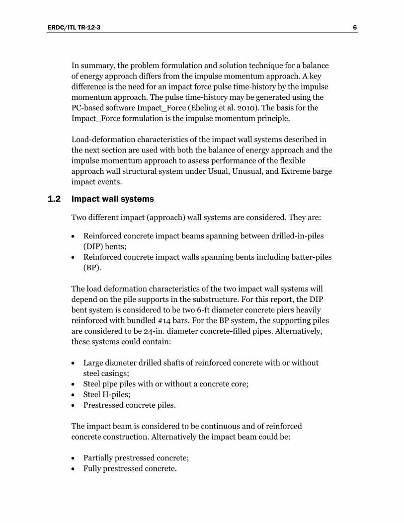
1.2 Impact wall systems
Two different impact (approach) wall systems are considered. They are:
Reinforced concrete impact beams spanning between drilled-in-piles (DIP) bents;
Reinforced concrete impact walls spanning bents including batter-piles (BP).
The load deformation characteristics of the two impact wall systems will depend on the pile supports in the substructure. For this report, the DIP bent system is considered to be two 6-ft diameter concrete piers heavily reinforced with bundled #14 bars. For the BP system, the supporting piles are considered to be 24-in. diameter concrete-filled pipes. Alternatively, these systems could contain:
Large diameter drilled shafts of reinforced concrete with or without steel casings;
Steel pipe piles with or without a concrete core; Steel H-piles; Prestressed concrete piles.
The impact beam is considered to be continuous and of reinforced concrete construction. Alternatively the impact beam could be:
Partially prestressed concrete; Fully prestressed concrete.

ERDC/ITL TR-12-3 7
Load-displacement related characteristics for the types of piles and impact beams described above will be discussed in Chapter 2 of the report.
1.3 Overview
The balance of energy approach requires that the initial kinetic energy (KE) acting normal to the impact wall of the approaching barge train is equal to the potential energy (PE), or strain energy, built up by deformation of the impact wall structural system when the normal barge train velocity becomes equal to 0.0.
A conservative approach is taken with respect to the balance of energy approach by assuming that all the barge train KE occurring in a direction normal to the wall must be converted to strain energy by the impact wall system. KE may be dissipated in other ways. With respect to low velocity impacts that occur when mooring ships to pile dolphins, which absorb the full energy of the moving vessel, it is assumed by Reese et al. (1970) that not more than half the ship’s KE will be transferred to the mooring structure. Other means for absorbing the total energy of the vessel include:
Deformation in the vessel itself (in the case of a barge train, the deformations of individual barges and the lashings that tie them together);
Hydraulic-related resistance when any change of angular velocity of the vessel occurs (this is also valid for a barge train);
Friction between the vessel and the impact structure (frictional forces occur in a direction tangent to the wall, but may affect the length of time for the barge train kinetic energy in a direction normal to the wall to be converted to the potential energy due to deflection of the wall).
However, little is known regarding other possible KE dissipation mechanisms with respect to higher velocity barge impact events. Therefore, no mechanism other than strain energy absorption by the impact wall system in a direction normal to the wall surface is considered in the balance of energy approach.
The impulse moment approach uses a pulse loading to represent the impact of a barge train with the wall. Peak displacement demands from the pulse loading response history are compared with wall displacement capacities. Both the balance of energy approach and the impulse moment approach lend themselves to a performance-based analysis. For the

ERDC/ITL TR-12-3 8
balance of energy approach, strain energy absorption must take place in a manner that represents a suitable response to Usual, Unusual, and Extreme barge impact events. For the impulse momentum approach, the peak displacement demand must take place within limits representing an acceptable response to Usual, Unusual, and Extreme barge impact events.
Upon barge impact, it is important that the approach wall cap beam distribute the potential energy and displacement demands to adjacent supports whether they are individual piles or caissons, vertical pile bents, or batter pile bents. Continuity of the cap beam is important for load sharing to take place. The relative stiffness of the cap beam to its support system will determine how the impact demands will be shared among supports.
Pushover analysis techniques are used to establish the potential energy capacity and displacement capacity of individual supports. The total stored energy (PE) of the approach wall system will be the sum of the stored energy of all the supports reacting to barge impact. To simplify the analysis with respect to bent supported systems, any strain energy absorbed by cap beam flexural deformation is ignored.
It is not possible to provide a unique barge impact loading that can be used for design purposes. The approach truly needs to be one that considers the balance of energy or impulse momentum analysis. It should be recognized that potential energy capacity and displacement capacity are a function of load-displacement response and that strengthening a system, if it means making the system stiffer, may not always be the most efficient way of meeting performance objectives.
1.4 Kinetic energy (KE)
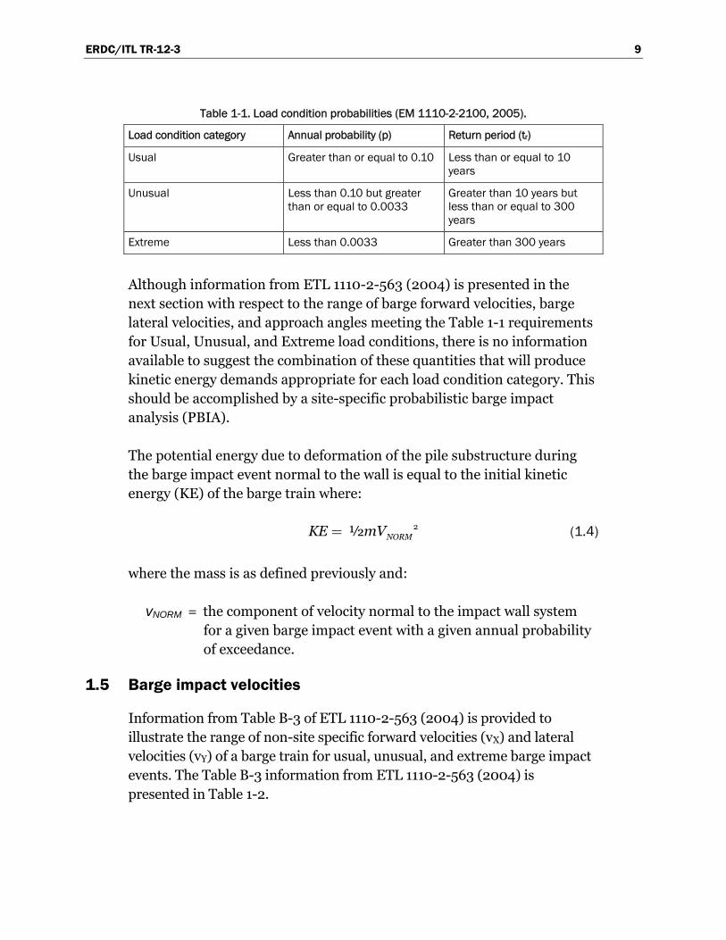
In the balance of energy approach and the impulse momentum approach, it is not only necessary to know the kinetic energy (KE) and displacement demands associated with a given barge train impact event, but also the probability of the event. Usual, Unusual, and Extreme events are defined in probabilistic terms per EM 1110-2-2100 (2005). Information regarding these three design loading categories from Table 3-1 of EM 1110-2-2100 (1991) is presented in Table 1-1.
ERDC/ITL TR-12-3 9
Table 1-1. Load condition probabilities (EM 1110-2-2100, 2005).
Load condition category Annual probability (p) Return period (tr)
Usual Greater than or equal to 0.10 Less than or equal to 10 years
Unusual Less than 0.10 but greater than or equal to 0.0033
Greater than 10 years but less than or equal to 300 years
Extreme Less than 0.0033 Greater than 300 years
Although information from ETL 1110-2-563 (2004) is presented in the next section with respect to the range of barge forward velocities, barge lateral velocities, and approach angles meeting the Table 1-1 requirements for Usual, Unusual, and Extreme load conditions, there is no information available to suggest the combination of these quantities that will produce kinetic energy demands appropriate for each load condition category. This should be accomplished by a site-specific probabilistic barge impact analysis (PBIA).
The potential energy due to deformation of the pile substructure during the barge impact event normal to the wall is equal to the initial kinetic energy (KE) of the barge train where:
2 ½ NORMKE mV= (1.4)
where the mass is as defined previously and:
vNORM = the component of velocity normal to the impact wall system for a given barge impact event with a given annual probability of exceedance.
1.5 Barge impact velocities
Information from Table B-3 of ETL 1110-2-563 (2004) is provided to illustrate the range of non-site specific forward velocities (vX) and lateral velocities (vY) of a barge train for usual, unusual, and extreme barge impact events. The Table B-3 information from ETL 1110-2-563 (2004) is presented in Table 1-2.

ERDC/ITL TR-12-3 10
Table 1-2. Non-site specific impact velocities for barge impact (ETL 1110-2-563, 2004).
Load Condition
Forward Velocity (VX) (fps)
Lateral Velocity (VY)
(fps)
Usual 0.5 – 2.0 0.01 – 0.1
Unusual 3.0 – 4.0 0.4 – 0.5
Extreme 4.0 – 6.0 > 1.0
The component of velocity normal to the approach wall can be determined if the impact angle is known. The relationship between barge train velocities and velocities normal and parallel to the flexible approach wall as related to the impact angle (θ) is illustrated in Figure 1-4.
Figure 1-4. Barge train and velocity vector transformation – from local barge train to global
(wall) axis (Arroyo-Caraballo and Ebeling (2006).

ERDC/ITL TR-12-3 11
1.6 Barge impact angle
The non-site specific impact angles for usual, unusual, and extreme events per Table B-4 of ETL 1110-2-563 (2004) are provided below in Table 1-3.
Table 1-3. Non-site specific impact angles for barge impact (ETL 1110-2-563, 2004).
Load Condition Approach Angle (θX) (deg)
Usual 5 - 10
Unusual 10 - 20
Extreme 20 - 35
1.7 Barge train size
Barge trains selected for use in probabilistic barge impact analyses (PBIA) often contain jumbo size barges. The weight of a single, ballasted jumbo barge may be obtained from Table A4 in Arroyo et al. (2003). This table is a summary of barge train weights used in the 1998 full-scale, low velocity, controlled barge impact experiments conducted at the decommissioned Gallipolis Lock at Robert C. Byrd Lock and Dam. The total tonnage weight for 15 barges is 29,125.35 tons ÷ 15 barges ≈ 1940 tons / barge. Information for a 2 x 2 barge trains, a 2 x 3 barge train, and a 3 x 3 barge train is presented in Table 1-4. Using information from Table A4 of Arroyo et al. (2003), an MVS JAR-Raike tow has a weight of 550 tons.
Table 1-4. Barge train weight and mass (Arroyo et al. 2003).
Barge Train Size
Barge Train Weight (kips)
Tow Weight (kips)
Total Weight Without Hydrodynamic Added Weight (kips)
Total Mass Without Hydrodynamic Added Mass (kip-s2 / ft)
2 x 2 15520 1100 16620 516
2 x 3 23280 1100 24380 757
3 x 3 34920 1100 36020 1118
Table 2.3 in Chapter 2 of Ebeling et al. (2010) provides additional information on barge train weights for different types of barges. Tow weights are also discussed in Section 2.3 of Ebeling et al. (2010).

ERDC/ITL TR-12-3 12
1.8 Hydrodynamic added mass
The components of barge mass including hydrodynamic mass normal to and parallel to the approach wall are determined as described in Equation 2-3 and 2-4 of ETL 1110-2-338 (1993). These are repeated below:
cos sin
X BARGE TRAIN Y BARGE TRAINNORM
X BARGE TRAIN Y BARGE TRAIN
m mm
M θ m θ- -
- -
·=
· + ·2 2 (1.5)
cos sin
X BARGE TRAIN Y BARGE TRAINPAR
Y BARGE TRAIN X BARGE TRAIN
m mm
M θ m θ- -
- -
·=
· + ·2 2 (1.6)
where mX-BARGE TRAIN and mY-BARGE TRAIN are the total barge masses (including hydrodynamic added mass) expressed in the local coordinate system of the barge train and:
.X BARGEM M- =1 05 (1.7)
.Y BARGEM M- =1 40 (1.8)
with M equal to the total mass of the barge train and tug without accounting for hydrodynamic mass.
1.9 Load factors
The load factors for usual, unusual, and extreme events, based on EM 1110-2-2104 (1992) and EM 1110-2-563 (2004) are provided in Table 1-5. These load factors are often the basis for original designs and indirectly establish the load-displacement characteristics of the impact wall system.
Table 1-5. Load factors for barge impact.
Load Condition Load Factor
Usual 1.7
Unusual 1.4
Extreme 1.1
1.10 Potential energy (PE) and displacement capacity
The strain energy due to deformation of a flexible approach wall system in response to a given barge impact event is defined as its potential energy

ERDC/ITL TR-12-3 13
(PE). The potential energy used in the balance of energy approach and the displacement capacity used in the impulse momentum approach is that associated with its force-deflection response, but does not include:
Energy lost to barge damage; Friction losses due to barge contact with the approach wall; Energy feedback (i.e. radiation feedback from the structure to the
foundation); Strain energy absorbed by the cap beam in flexure (flexible bent
systems); Energy dissipation due to the swing of the vessel (Equation B-2
COM624G Users Manual).
1.11 Performance objectives
Performance-based design techniques are used to evaluate approach wall systems for barge impact loads. Three performance levels are to be considered when evaluating the response of approach walls to barge impact events: serviceability performance, damage control performance, and collapse prevention performance. The premise of the performance-based approach is that a greater risk of damage can be tolerated when the probability of event occurrence is low. Therefore serviceability performance is required for usual barge impact events, damage control performance is required for unusual barge impact events, and collapse prevention performance is all that is required for extreme barge impact events.
1.11.1 Serviceability performance
The structure is expected to be serviceable and operable with no damage (linear elastic performance) for barge impact loadings that have return periods of 10 years or less (usual loading). For the usual design event, the maximum displacement of the approach wall will have a load-displacement response at the upper limit of the linear elastic range (i.e., before the first yield mechanism develops). The potential energy (PE) of the approach wall system under usual load conditions is limited by this maximum displace-ment.
1.11.2 Damage control performance
Elements of the approach wall system can perform near or beyond first yield for barge impact loadings that have return periods between 10 years and

ERDC/ITL TR-12-3 14
300 years (unusual loading) provided damage is minor and repairable. Damage should be concentrated in discrete locations above the mud line to achieve the performance goal of being easily repairable and having economically feasible repairs.
1.11.3 Collapse prevention performance
Collapse prevention performance requires that collapse of the structure be prevented and that the load capacity be substantially undiminished for barge impact loadings that have return periods greater than 300 years (extreme loading). Damage may be significant and difficult to repair, but should be limited to regions above the mudline to make damage assessment possible.
The above performance objectives are illustrated by load-deflection curves for a DIP system Figures 1-5 (a, b, and c).
The above performance objectives are illustrated by using the Figures 1-6 (a, b, and c) example taken from the load-deflection curve of a pushover analysis made for a BP system. This pushover analysis will be discussed in detail in Chapter 4 and Appendix B.
1.12 Load sharing
It is important to remember that barge train impact loading may be shared by nearby supporting pile bents, depending on the structural details of the impact beam or impact deck. With structural continuity provided through the structural detailing of the impact superstructure, load sharing among the pile groups can be achieved. In this case, pushover analyses and the establishment of potential energy (PE) capacity for a particular pile bent represents only a fraction of the energy delivered to the impact wall system. Impact effects will be shared between adjacent bents based on several factors including:
Cap beam continuity (simply supported or continuous); Relative flexibility of the cap beam with respect to its support system; Impact location; Boundary conditions at approach wall end supports.
Distribution of barge impact to adjacent bents should be evaluated using a 3-D analytical model similar to that shown in Figure 1-7.

ERDC/ITL TR-12-3 15
Figure 1-5a. Load versus displacement plot for fixed-head bent - Serviceability performance of the usual load case.
Impact at various locations that can place maximum kinetic energy (KE) demands on the pile bents and cap beam should be investigated. The cap beam should be investigated for displacement actions associated with flexure and force-controlled actions associated with shear.
1.13 Pushover analysis and force-deflection response
The potential energy (PE) absorption capacity, as represented by the load deformation characteristics of impact wall systems, will be determined by pushover analysis. The pushover method defines the path of least energy resistance and the area under the load-displacement diagram approximates the energy absorption capacity of the system. The pushover analysis described below applies to an individual support. Its use in the design of an

ERDC/ITL TR-12-3 16
individual pile group for vertical (i.e. plumb) piles is discussed in Chapter 3 and in Chapter 4 for a batter pile group system. Flexible impact beams that are simply supported by either type of pile group are envisioned for these cases. Its use in the design of an approach wall system containing many supports and with sufficient structural detailing contained within the superstructure to accommodate load sharing is described in Chapter 5.
Figure 1-5b. Load versus displacement plot for fixed-head bent - Damage control performance of the unusual
load case.

ERDC/ITL TR-12-3 17
Figure 1-5c. Load versus displacement plot for fixed-head bent - Collapse prevention performance of the
extreme load case.
1.13.1 Origin of pushover analysis in earthquake engineering
Pushover analyses were introduced in earthquake engineering to reconcile the capacity of a structure such as a building or bridge with the demands of an earthquake as represented by an elastic response spectrum. This methodology was first designated as the capacity spectrum method and used by the Corps to evaluate the ability of buildings to withstand major earthquakes (TM 5-809-10.1 1986). The construction of the capacity curve is accomplished using pushover analysis techniques and is therefore of interest for this report. In TM 5-809-10.1 (1986) the capacity curve is developed in a step-by-step procedure using superposition, where the

ERDC/ITL TR-12-3 18
Figure 1-6a. Load versus displacement plot for BP bent - Serviceability performance.
Figure 1-6b. Load versus displacement plot for pipe pile system - Damage control performance.

ERDC/ITL TR-12-3 19
Figure 1-6c. Load versus displacement plot for pipe pile system - Collapse prevention performance.
structure is laterally distorted to some limiting capacity value, frozen in that position, local yielding elements are relaxed, and the structure is laterally distorted to the next limiting capacity value. The procedure is repeated until the structure has reached a limit state consistent with an established performance objective. The procedure is illustrated in Priestley et al. (1996) with respect to a bridge bent where the displacement response is limited by flexure.
1.13.2 Incremental analysis technique for barge impact loading in a pushover analysis
In a pushover analysis for barge impact, suitable analytical models are developed and a barge impact load is applied in increasing increments until first yield occurs. The yielding element is relaxed and the process repeated until all yield mechanisms have formed and a potential collapse mechanism develops. A collapse mechanism is considered to exist when the most critical element has reached its ultimate rotational capacity, axial capacity, or foundation support capacity. Brittle failure mechanisms (shear, etc.) should be monitored during the pushover analysis to assure that performance objectives associated with the assumed limiting response

ERDC/ITL TR-12-3 20
Figure 1-7. Analysis of 3-D effects due to sharing of the impact load among pile groups.
are not compromised. The pushover technique used will be dependent on the characteristics of the particular approach wall system. Descriptions of pushover analysis techniques contained in this report are not intended to be prescriptive with respect to analytical modeling or with respect to the sequence of failure mechanisms. The pushover analysis technique with respect to DIP bent and BP bent systems are summarized in Chapters 3 and 4, respectively, of this report. Details of the pushover analysis example for a DIP bent system is provided in Appendix A. Details of the pushover analysis example for a BP bent system are provided in Appendix B.

ERDC/ITL TR-12-3 21
To capture hinge formation sequencing and proper load displacement response it is necessary to use analytical techniques that account for pile-soil interaction effects. Three analytical techniques that account for pile-soil interaction effects are:
Yang (1966) approach Saul (1968) approach Nonlinear p-y curve approach
These techniques are discussed in detail in Chapters 3 and 4 of this report.
1.14 Non-linear conservation of energy
A pushover analysis of a pile-based flexible system proceeds until the barge train velocity is reduced to 0.0 fps normal to the approach wall. This is the point where the barge train’s kinetic energy normal to the wall has been fully converted to the potential energy of the pile-based, flexible system as a result of the deformations of the piles and the beam. During this pushover analysis, the pile-based system undergoes mechanisms (e.g., flexural yielding of the pile at the pile cap) that affect the rate with which potential energy can be stored, resulting in a non-linear curve as shown in Figure 1-8. For the pile-based, flexible system to survive the impact, the normal displacement at the superstructure of the pile based system should not reach the point where any of the piles form a plastic hinge beneath the mudline. Repair of a “hinge” may be accommodated above water but is prohibitive below the mudline.
The Potential Energy of the pile-based flexible system contained within the Figure 1-8 load-deflection relationship represents the conclusion of the first stage of the impulse as defined in terms of the Kinetic Energy of the barge train during its initial contact until the velocity of the barge train normal to the wall has been reduced to 0.0 fps. The “unload” stage of the impulse releases a portion of the stored potential energy from the pile group, accelerating the barge train in the opposite direction along the wall normal. The pushover analysis does not proceed into the “unload” stage of the pile response because, at this point, the peak deflection (and peak potential energy) has occurred in the system and a determination of whether a plastic hinge will form below the mudline can be made.

ERDC/ITL TR-12-3 22
Figure 1-8. Load-displacement plot for fixed-head bent.
1.15 Report contents
Chapter 2 discusses the analytical models that represent drilled-in-place and batter pile bents (or group of piles). These models allow the user to establish capacities, limits, fixities, and the stiffness of the pile system. Failure mechanisms are discussed as they relate to each pile group model.
Chapter 3 discusses the details regarding the pushover analysis for vertical pile bent systems. The pushover analysis is introduced as a method to define the load versus displacement relationship for a single pile group and thus establish the potential energy capacity for the specific pile group configura-tion being analyzed. Loading is applied incrementally so as to establish specific failure mechanisms within the pile group and therefore, accurately

ERDC/ITL TR-12-3 23
define the load versus deflection curve. Yielding of individual piles (e.g., below the mud line), flexural failure of connections of pile to the pile cap, failure of the soil by pull-out, or soil bearing failure due to pile plunging are constantly being evaluated during the incremental analysis. Each failure mechanism affects the load versus deflection curve for the pile-based system. Various methods to define the required length of vertical (i.e., plumb) piling founded in different soil and rock types are discussed. There is also a discussion of how these pushover analyses can be used to optimize the structure (i.e., the length of piles). Attention is also paid to pile-soil interactions considering proximity effects between piles.
Chapter 4 continues the discussion of pushover analysis, but for batter pile systems. A discussion is given about the limitations of analytical models in this situation, and the efficiencies and deficiencies of batter pile systems. The physical limitations of placement for batter piles are also taken into consideration.
Chapter 5 discusses a 3-D analytical procedure to account for load sharing among the pile groups when the impact beam (or impact deck) is struc-turally detailed to accommodate this behavior. In this type of 3-D structural system model, impact loading does not have to be specified at the center-line of an individual pile bent but can be specified anywhere along the impact superstructure. The distribution of loading between the impact superstructure and the substructure (consisting of multiple pile groups) is discussed, as well as the interactions occurring between the super- and sub-structural elements.
Chapter 6 provides the conclusions of the research conducted to-date, summarizes the viability of the analytical tools used during the course of this research, and describes the next stages of Research & Development that extend the capabilities of analyzing flexible approach wall systems containing a flexible, pile-based substructure.
Appendix A provides the example pushover analyses based on proposed designs for vertical pile systems that pertain to Chapter 3. Inputs for the different analytical models and the corresponding software (e.g., CPGA, COM624G, etc.) are presented.

ERDC/ITL TR-12-3 24
Appendix B provides example pushover analyses based on proposed designs for batter pile systems that pertain to Chapter 4. Inputs for the analytical models and the CPGA software are presented.
Appendix C provides the example pushover analyses based on proposed designs for batter pile systems that pertain to Chapter 4. Inputs for the analytical model and the GROUP7 software are presented.
Appendix D provides guidance for the determination of skin friction and tip capacities of piles and pile groups founded in clay and sand.
Appendix E discusses the fact that impacts with flexible pile-founded structures are dynamic events. A discussion is provided for how these dynamic events are largely affected by the geometry of beams and place-ment of piles and bents in a multi-degree of freedom (MDOF) system. Procedures for computing modal periods for various pile founded substructures are presented.

ERDC/ITL TR-12-3 25
2 Analytical Models For Drilled-In Place And Batter Piles
2.1 Introduction
Analytical models to be used in the (1) balance of energy approach and (2) the dynamic response analysis of the flexible approach wall to a pulse force time-history vary in complexity. Simplified analytical models are often used in preliminary analyses but more comprehensive analytical models are often required for final designs of flexible approach walls or in the evaluation of existing approach walls.
Demand: The impact demand is characterized in terms of the kinetic energy normal to the approach wall in engineering methodologies presented in this report. For the dynamic response analysis of the wall approach, the kinetic energy demand is transformed to a pulse force time-history using the method outlined in Ebeling et al. (2010).
Capacity: Capacity methods are needed to determine potential yield levels. Capacity can be governed by the strength of the materials used in the piles or pile cap, and/or can be governed by the capacity of the (soil or rock) founda-tion to support the piles. Force-displacement relationships depend on the yield and ultimate strain characteristics of the structure and its foundation. These relationships become nonlinear after yield levels are exceeded.
This chapter will focus on analytical models, capacities, and load-displacement characteristics of elements that comprise drilled-in-pile (DIP) bent systems and batter-pile (BP) bent systems. Elements include partially embedded piles, cap beams, and foundation materials.
2.2 Drilled-in-pile (DIP) bent systems
Large diameter, vertical drilled-in piles can be used to support approach wall structural systems. Piles are a minimum of 2.5 ft in diameter, but more commonly they range from five to seven ft in diameter and can be as large as 10 ft in diameter. Excavation is usually accomplished by drilling. Generally, a steel casing 3/8 to 1/2 in. thick is installed to protect against collapse or cave-in of the side walls. Reinforcing steel is inserted into the casing protected shaft and the shaft is filled with concrete. Drilled-in

ERDC/ITL TR-12-3 26
caissons systems used to support approach walls are heavily reinforced to provide the moment capacity needed to resist barge impact loadings. Design and construction procedures for drilled-in caisson systems are described in ACI Committee Report 336 (1972), “Suggested Design and Construction Procedures for Pier Foundations”. The characteristics important to the balance of energy approach and the dynamic response analysis of the flex-ible approach wall to a pulse force time-history are the displacements at the point of barge impact as a function of the barge impact load. This requires knowledge about the effective stiffness (EI) of the flexural system and the spread of plasticity (plastic hinge length) as the system nears its ultimate (structural) displacement capacity.
A typical DIP bent system and its response to barge impact loadings is illustrated in Figure 2-1. The DIP system considered in this chapter is a two-pile bent system with moment fixity at the pile-to-pile cap connection. Other types of multiple rows of vertical pile systems may be analyzed by adapting the engineering procedure discussed in this chapter.
Figure 2-1. DIP bent system.
ERDC/ITL TR-12-3 27
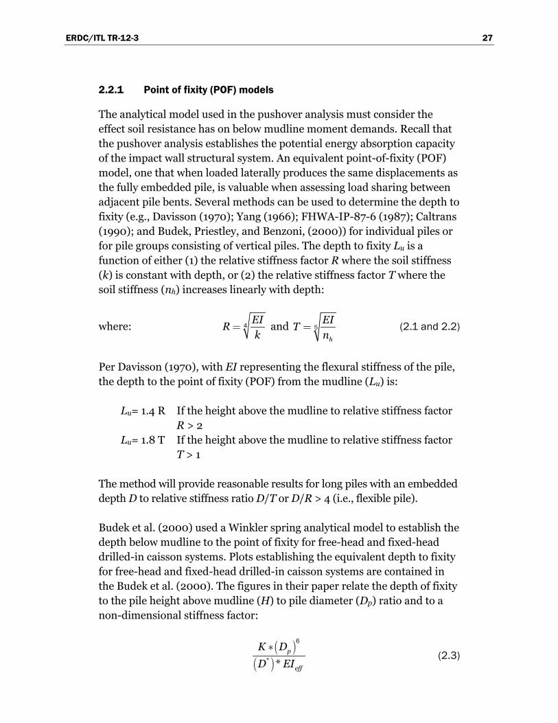
2.2.1 Point of fixity (POF) models
The analytical model used in the pushover analysis must consider the effect soil resistance has on below mudline moment demands. Recall that the pushover analysis establishes the potential energy absorption capacity of the impact wall structural system. An equivalent point-of-fixity (POF) model, one that when loaded laterally produces the same displacements as the fully embedded pile, is valuable when assessing load sharing between adjacent pile bents. Several methods can be used to determine the depth to fixity (e.g., Davisson (1970); Yang (1966); FHWA-IP-87-6 (1987); Caltrans (1990); and Budek, Priestley, and Benzoni, (2000)) for individual piles or for pile groups consisting of vertical piles. The depth to fixity Lu is a function of either (1) the relative stiffness factor R where the soil stiffness (k) is constant with depth, or (2) the relative stiffness factor T where the soil stiffness (nh) increases linearly with depth:
where: EI
Rk
= 4 and h
EIT
n= 5 (2.1 and 2.2)
Per Davisson (1970), with EI representing the flexural stiffness of the pile, the depth to the point of fixity (POF) from the mudline (Lu) is:
Lu= 1.4 R If the height above the mudline to relative stiffness factor R > 2
Lu= 1.8 T If the height above the mudline to relative stiffness factor T > 1
The method will provide reasonable results for long piles with an embedded depth D to relative stiffness ratio D/T or D/R > 4 (i.e., flexible pile).
Budek et al. (2000) used a Winkler spring analytical model to establish the depth below mudline to the point of fixity for free-head and fixed-head drilled-in caisson systems. Plots establishing the equivalent depth to fixity for free-head and fixed-head drilled-in caisson systems are contained in the Budek et al. (2000). The figures in their paper relate the depth of fixity to the pile height above mudline (H) to pile diameter (Dp) ratio and to a non-dimensional stiffness factor:
( )
( )* *p
eff
K D
D EI
*6
(2.3)

ERDC/ITL TR-12-3 28
where:
K = subgrade reaction modulus (force per length3); Dp = Diameter of drilled-in caisson; D* = the “standard” pile diameter of 6 ft (1.83 m); EIeff = Effective (cracked section) stiffness of caisson.
Observe that the depth to the point of fixity is a function of the ratio of the soil stiffness divided by the flexural stiffness of the pile. This topic is discussed in further detail in Chapter 3.
2.2.2 Analytical models suitable for pushover analyses
Analytical models are needed for use in pushover analyses so as to establish the potential energy (PE) capacity and displacement capacity of drilled-in pile bent systems. A key aspect of the analytical models being used is that they include the computation of structural displacements. The area under the load-deflection curve, as established by pushover analysis, represents the PE capacity. The analytical models with capacity to account for the influence of below mudline soil resistance are described in Chapters 3 and 4 of the report. For flexible approach walls with vertical piling (Chapter 3), linear p-y curve pushover analysis can be accomplished using the Yang (1966) Method or the Saul (1968) Method (i.e., Corps CPGA computer program, X0080). Nonlinear p-y curve pushover analysis can be performed for drilled-in piles using the Corps COM624G computer program, I0012. The pushover analysis is accomplished using CPGA for batter pile groups (Chapter 4).
2.2.3 Capacity
For properly designed bent systems, pile yielding will occur in flexure due to lateral impact loading of the deck, impact beam or impact skirt of the approach wall. The engineering evaluations conducted while preparing this report indicates that initial flexural yielding will occur at the pile to pile cap connection. With additional lateral loading, this will be followed by flexural yielding at the point of maximum moment below the mudline.
Flexural yielding at each of the potential yield locations described above can be assumed to occur when the pile reaches it nominal (yield) capacity in flexure. The axial load ratio in large diameter drilled-in caissons is likely to be low and therefore the nominal moment capacity can often be
ERDC/ITL TR-12-3 29
assumed as that associated with pure bending. This nominal moment capacity can be determined by moment-curvature analysis. The Corps CASE program M-PHI (X2002) can be used for this. Alternatively, the nominal moment capacity can be determined by constructing the axial load-moment interaction diagram. This process is illustrated with respect to the DIP and BP bent system analyses. The Corps CASE program CGSI (X0061) can be used to construct the interaction diagram for drilled-in caissons. Often simple hand calculations can be made to establish critical points on the interaction diagram.
2.2.4 Displacement limit state
After the below mudline flexural yield mechanisms take place, the post-yield displacement capacity associated with plastic hinge rotation (θp) can be estimated. Displacement associated with below mudline plastic rotation is assumed to occur without significant increase in lateral load. The plastic hinge rotation capacity for reinforced drilled-in caissons can be estimated using procedures described in Budek et al. (2000). This process requires a moment-curvature analysis to obtain the ultimate curvature capacity and the curvature capacity at first yield. The plastic rotation and associated displacement capacity can be determined with this information and knowledge about the extent of yielding (plastic hinge length). The additional (structural) displacement capacity due to below mudline plastic hinge rotation, however, may not be important with respect to meeting estab-lished performance objectives; damage associated with this type of pile performance below the mud line is costly to repair and therefore, will not satisfy the Corps performance objectives for usual and unusual loading.
2.2.5 Effective stiffness
To properly assess the potential energy (PE) capacity of DIP bent systems, a reasonable estimate of the (structural) system displacement must be deter-mined for each increment of lateral loading. For DIP and other bent systems containing reinforced concrete piles, this is best accomplished using cracked section stiffness rather than gross section stiffness, since the gross section stiffness can significantly underestimate the displacement response. Formulations provided by Priestley in Appendix G, Section G.2 of Strom and Ebeling (2005) are proposed for use in estimating the deflection response of drilled-in piles subjected to barge impact loading. The effective moment of inertia, Ieff, of reinforced concrete piles at near yield conditions can be significantly less than that represented by the gross section moment

ERDC/ITL TR-12-3 30
of inertia, IG. The effective moment of inertia is an average value for the entire pile and considers the distribution of cracking along the pile length. The effective moment of inertia of reinforced concrete piles can be esti-mated based on the relationship between the cracking moment MCR (i.e., the moment required to initiate cracking while ignoring the reinforcing steel) and the nominal moment capacity MN of the reinforced concrete pile section. The nominal moments and cracking moments used to estimate effective moment of inertia are for those regions where moments are at their maximums. For caissons, this will be near the point of fixity and/or pile to cap connection. Once the cracking moment MCR and the nominal moment capacity MN for the pile have been determined the ratio of the effective moment of inertia Ieff to the gross moment of inertia IG can be estimated as follows:
. .eff N
G CR
I M
I M
é ùê ú= - -ê úë û
0 8 0 9 1 (2.4)
The ratio of Ieff/IG shall not be greater than 0.8, nor less than 0.25 for Grade 60 steel, or less than 0.35 for 40 Grade steel.1 The nominal moment strength can be determined in accordance with standard ACI 318 (2002) procedures using moment-curvature analysis, or axial/moment interaction analysis. The cracking moment MCR can be determined by the following expression:
CR r b
PM f S
A
æ ö÷ç= + ÷ç ÷çè ø (2.5)
where:
f r = Modulus of rupture = '5.7 cf (psi units)
P = Axial load (pounds) A = Area (in2) Sb = IG/c = Section modulus (in3)
Equation 2-4 is a simplification of the Bronson Equation as described by Priestley in Appendix G, Section G.2 of Strom and Ebeling (2005). Drilled-in piles generally have longitudinal steel reinforcing ratios that are high (2-3 percent) and therefore it is likely that the effective moment of inertia Ieff
1 Refer to Appendix G, Section G.2 in Strom and Ebeling (2005).

ERDC/ITL TR-12-3 31
will be at its minimum (25 percent of IG for 60 grade steel and 35 percent of IG for 40 grade steel).1
2.3 BP bent systems
Batter pile (BP) bent systems can be open-end pipe piles, H-piles, or prestressed concrete piles. Open-end pipe piles are steel pipe piles installed with the bottom end open. Wall thicknesses range from ¼ to ½ in. Open end pipe piles may be installed by driving or jacking. For maximum bearing capacity they are installed to rock, cleaned out and filled with concrete. H-piles are heavy steel pile sections that are typically driven to obtain the required bearing capacity. Prestressed piles are generally pretensioned. The prestressing is used to overcome tensile stresses that can develop in the pile under certain driving conditions.
An example BP bent system is illustrated in Figure 2-2. The BP system considered in this report consists is a three-pile bent system with two batter piles and a single vertical pile. Piles are 24-in. diameter concrete-filled pipe piles. Pile groups are spaced on six ft six in. centers along the flexible approach wall. Moment fixity is assumed to be provided at the pile to pile cap connection.
Figure 2-2. BP bent.
1 Refer to Appendix G, Section G.2 in Strom and Ebeling (2005).

ERDC/ITL TR-12-3 32
The response of batter pile systems to barge impact loadings is varied with respect to the formation of yield mechanisms and the sequence in which they form. The structural system response depends upon the structural configuration and the structural members and foundation soil(s) properties. One possible scenario is illustrated in the Appendix B example and summarized in Chapter 4.
2.3.1 Analytical models
Unlike all-vertical piling systems (e.g., Figure 2-1), flexural yielding in a batter-pile bent system may not be as important as its response to axial tensile and axial compressive loads. Since the piles in a batter pile bent system are partially embedded it is necessary to account for the load-deformation effects associated with the pile section above the mudline as well as that below the mudline.
Since the axial stiffness of the various piles in a batter pile bent system can have significant influence on the response of the system to lateral barge impact forces, a spring model that captures soil-pile interaction effects, similar to that described in EM 1110-2-2906 (1991) and illustrated in Figure 2-3 for compression and tension piles, is recommended for the final barge impact evaluation of batter pile bent systems.
Figure 2-3. Pile axial behavior and spring model.
End Bearing
Axial Compressive Load
Axial Tensile Load
Axial Stiffness of Pile (AE)
Shear Resistance of Soil
Tension Pile Compression Pile
ERDC/ITL TR-12-3 33
As described in Chapter 4 of the report, the Saul (1968) method, implemented in the Corps computer program CPGA (X0080), is useful when performing pushover (load-displacement capacity response analyses) of batter pile bents. Although restricted to rigid pile caps and linear p-y curves, it can accommodate batter pile systems that are cantilevered above the mudline. COM624G (Corps computer program I0012) although having nonlinear p-y capability is limited to the evaluation of a single vertical pile. CPGA has the ability to accommodate axial and flexural stiffness values determined by comprehensive analysis, or load testing thereby making useful for both preliminary and final analysis.
2.3.2 Axial and flexural capacity
The axial capacity of the pile can be governed by the strength of the materials that make up the pile, the buckling capacity of the pile, or the capacity of the soils that support the pile. Flexural capacity will be governed by the strength of the materials that make up the pile.
2.3.3 Pile axial and flexural interaction capacity effects
Limited engineering evaluations conducted during the preparation of this report indicate that it is unlikely that the axial capacity of the pile will be governed by the strength of the materials that make up the pile (for normal-sized piles used on Corps approach wall projects). However, this is not true for flexure. Since the axial load in the pile will influence its flexural capacity, interaction diagrams should be constructed for the type (or types) of piles used in the batter pile bent system. The construction of the axial load / moment diagram can be accomplished in a simple manner using manual calculations to identify various control points, or by computer programs to generate a complete interaction curve.
2.4 Simple interaction diagrams for piles
Simple interaction diagrams can be developed for drilled-in caisson (concrete) piles and the various types of piles (steel open-end pipe piles, concrete-filled pipe piles, steel H-piles, and prestressed concrete piles) used in batter pile bent systems. Corps computer programs are available to develop the complete interaction diagram for concrete and prestressed concrete piles (Corps CGSI program X0061 and Corps CPGC program X0088), which may be a better choice considering the complexity in establishing the pure moment capacity for circular sections. With the
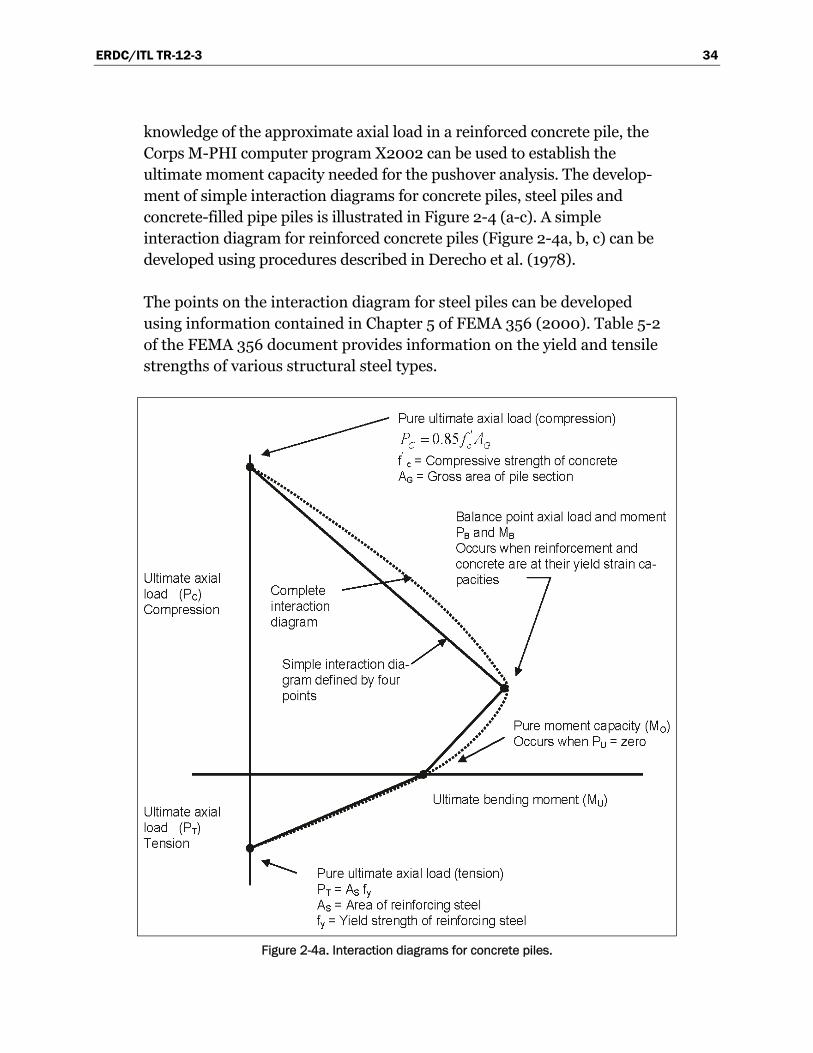
ERDC/ITL TR-12-3 34
knowledge of the approximate axial load in a reinforced concrete pile, the Corps M-PHI computer program X2002 can be used to establish the ultimate moment capacity needed for the pushover analysis. The develop-ment of simple interaction diagrams for concrete piles, steel piles and concrete-filled pipe piles is illustrated in Figure 2-4 (a-c). A simple interaction diagram for reinforced concrete piles (Figure 2-4a, b, c) can be developed using procedures described in Derecho et al. (1978).
The points on the interaction diagram for steel piles can be developed using information contained in Chapter 5 of FEMA 356 (2000). Table 5-2 of the FEMA 356 document provides information on the yield and tensile strengths of various structural steel types.
Figure 2-4a. Interaction diagrams for concrete piles.

ERDC/ITL TR-12-3 35
Figure 2-4 b. Interaction diagram for steel piles.
The simple interaction diagram for steel piles (Figure 2-4b) does not include P•Δ or buckling effects. The effect lateral deflection has on pile axial compressive capacity will be discussed later.
The interaction diagram for concrete-filled pipe piles can be developed using procedures described in Ragan and Joyce (1992). A similar approach can be used to develop a simple interaction diagram for a concrete-filled pipe pile. This process is illustrated in Figure 2-4c.
Knowing the axial load on the pile, interaction diagrams similar to those illustrated in Figure 2-4 (a, b, and c) can be used to estimate pile moment capacities. The pile moment capacity is helpful to determine when, or if, flexural yielding will occur.

ERDC/ITL TR-12-3 36
Figure 2-4 c. Interaction diagrams for concrete-filled pipe piles.
2.5 Buckling effects on pile capacity
During the pushover capacity analysis, it is possible that the displacement of the batter pile bent systems will reach limits where pile buckling is possible after local yielding occurs. Second-order displacements can reduce axial load capacity and eventually cause a pile or group of piles to buckle. A simple procedure for evaluating second-order displacement effects on piles is described in Yang (1966). This information is presented in Chapter 3 of the report. This issue is of concern for standard sized piles that extend (cantilever) above the mud line and is of greater concern if they are embedded in soils which possess low shear strength and low lateral stiffness in the region immediately below the mud line.

ERDC/ITL TR-12-3 37
2.6 Flexural hinge rotational capacity of piles
It is unknown whether or not the ultimate rotational capacity and assoc-iated (structural) displacement capacity will be important with respect to meeting established performance objectives. The ultimate rotational capa-city of flexural hinges in the piles of batter pile bent systems will depend on whether the member is of reinforced concrete, prestressed concrete, or steel. The method used to determine the ultimate rotational capacity of reinforced concrete members, which can include drilled-in caissons and other reinforced concrete piling is as described in Budek et al. (2000).
Prestressed concrete piling with conventional W3.5 spiral steel spaced at 6-in. is subject to sudden brittle failures at curvatures between 2.5 x 10⁻⁴ in-1 and 3.0 x 10⁻⁴ in-1 (Sheppard 1983). Prestressed concrete piling specially reinforced with W3.5 spiral steel spaced at 1.5-in. (percent spiral reinforce-ment equals 1.2 percent; ρs = 0.012) exhibit ductile performance with curvatures of about 6.0 x 10⁻⁴ in-1 (Sheppard 1983). Assuming a plastic hinge length (Lp) equal to the pile cross-sectional dimension (width for square piles, diameter for circular piles, etc.) the rotational capacity for various size conventionally reinforced and specially reinforced piling is as indicated in Table 2-1.
Table 2-1.Plastic rotation capacity for prestressed piles square, round, and octagonal sizes varying from 10 – 36 in. conventional and special transverse reinforcement
Size (in.)
Plastic Rotation Capacity (θ) Conventional Reinforcement
Plastic Rotation Capacity (θ) Special Reinforcement
10 0.0025 0.0060
12 0.0030 0.0072
14 0.0035 0.0084
16 0.0040 0.0096
18 0.0045 0.0108
20 0.0050 0.0120
24 0.0060 0.0144
30 0.0075 0.0180
36 0.0090 0.0216

ERDC/ITL TR-12-3 38
Note that Table 2-1 assumes
a curvature capacity of 2.5 x 10⁻⁴ in-1 for conventional transverse reinforcement
a curvature capacity of 6.0 x 10⁻⁴ in-1 for special transverse reinforcement
The plastic rotational capacity (θ) of steel pipe piles and H-piles can be determined using information contained in Table 5-6 of FEMA 356 (2000). Information pertinent to the pushover analysis of steel piling is shown in Table 2-2.
Table 2-2. Rotational capacity (θ) for collapse protection performance steel piles controlled by flexure.
f
f ye
b
t F£
522
and
w ye
ht F
£300
Plastic Rotation Angle (θ) Radians 9 θy
f
f ye
bd
t F³
652
or
w ye
ht F
³460
Plastic Rotation Angle (θ) Radians 4 θy
where:
bf = Flange width (in.); tf = Flange thickness (in.); h = Distance from inside compression flange to inside tension
flange (in.); Fye = Expected yield strength (psi).
( )ye c
yc ye
Z F I Pθ
EI P
æ ö÷ç ÷= -ç ÷ç ÷çè ø1
6 Yield rotation – Piles (2.10)
Z = Plastic section modulus; Ib = Moment of inertia for beam;
ERDC/ITL TR-12-3 39
Ic = Moment of inertia for column; E = Modulus of elasticity; P = Axial force on column; Pye = Expected yield axial strength of column.
2.7 Cap beams
The capacity of concrete cap beams in flexure and shear can be determined using methods described in ACI 318 (2002) and modified for older struc-tures as described in Appendices A and B of Strom and Ebeling (2005). In most instances when impact beams are on a deformable bent system all yield mechanisms will take place in the supporting bent system.
The ultimate rotational capacity for concrete cap beams that are fully prestressed, partially prestressed, or conventionally reinforced can be determined by:
cue
εθ d
c= (2.11)
where:
εcu = Ultimate strain capacity of concrete (0.0030);
c = depth from extreme fiber in compression to neutral axis; de = depth to tensile force in steel.
Using Naaman’s formulation as presented in Skogman et al. (1988)
ps ps ps ns y nse
ps ps ns y
A f d A f dd
A f A f
+=
+ (2.12)
where:
Aps = Area of prestressing steel; Ans = Area of non-prestressed (conventional) reinforcement; fps = Ultimate strength of prestressing steel; fns = Ultimate strength of non-prestressed (conventional)
reinforcement; dps = depth to tensile force in prestressing steel; dns = depth to tensile force in non-prestressed (conventional)
reinforcement.

ERDC/ITL TR-12-3 40
In Naaman’s formulation:
.e
cd
£0 425 (2.13)
This means the minimum plastic rotation capacity for a cap beam will be:
min . ..
cue
εθ d
c= = =
10 003 0 007
0 425
Barge impact can occur anywhere along the cap beam (i.e., approach wall). A key impact case to be investigated when evaluating flexure is the case where the cap beam will be impacted at center span where the moment demand is at a maximum. The magnitude of maximum flexural demand will depend on whether the cap beam is continuous or simple span, whether contraction/construction joints are keyed or unkeyed, and whether the support system is flexible or rigid. Barge impact distribution effects are examined in Chapter 5. When evaluating shear, a key impact case to be investigated is where a barge impact occurs near a support where shear will be at a maximum. Shear is considered to be a force-controlled action and as such the shear capacity of the cap beam should exceed the shear demand. This and other force-controlled actions are discussed in Section 4.1 of Strom and Ebeling (2005).

ERDC/ITL TR-12-3 41
3 Pushover Analysis of Drilled-In-Pile Bent Systems
3.1 Introduction
This chapter discusses the evaluation of drilled-in-place (DIP) bent systems using a pushover analysis. This research effort adapts the push-over analysis to the analysis of deformable (i.e., flexible) approach walls for the problem of dynamic loading that occurs during barge impacts. The pushover analysis was first developed by the earthquake structural engineering community. It was initially presented in TM 5-809-10.1 (1986) as a capacity spectrum method for use in evaluating the seismic performance of buildings. It later appeared in FEMA 356 (1997) as a nonlinear static analysis procedure to be used for the seismic evaluation of existing buildings. A pushover analysis approach with respect to bridge support systems is described in Priestley et al. (1996) A pushover analysis is a deformation based earthquake engineering procedure that explicitly accounts for nonlinear, plastic, and limiting material and structural performance of individual structural members that comprise the structural system. Nonlinear structural performance is accounted for in the deforma-tion analysis with a limiting case corresponding to the collapse of the structural system (should the earthquake loading be so severe so as to cause a collapse mechanism to form within the structural system). The results of a pushover analysis of deformable approach walls are used to establish the capacity of the structural system to barge impact loadings.
3.2 Formulation of a pushover example problem
The example problem in this chapter is a vertical pile system designed for a guard wall constructed of 34-ft-wide and 81-ft-long bent sections. Each section is supported by three groups of six-ft-diameter, drilled-in-pile caissons. The pile groups are separated by 27 ft from centerline to centerline. The normal component of the barge impact force acts in a direction along the line of the pile group, as shown in Figure 3-1.
Figure 3-2 shows a section view of the loaded pile group and the supported bent structure. The piles are fixed into the bent, allowing for no rotation at the pile cap. For the example problem, the piles are exposed for 40 ft from the base of the bent to the top of the sand (i.e., the “unembedded”

ERDC/ITL TR-12-3 42
Figure 3-1. Plan view of the vertical drilled-in-pile pushover example problem.
Figure 3-2. Section view of bent supported by two vertical piles embedded in sand.

ERDC/ITL TR-12-3 43
length, Lu). The complete pushover analysis of this flexible approach wall structure using Yang, COM624G, and CPGA methods is described in detail in Appendix A.
3.3 Determination of minimum embedment depth
One of the fundamental design issues for a laterally loaded vertical pile or group of vertical piles, and a prerequisite to a pushover analysis, is establishing the minimum depth of embedment (i.e., depth of penetration below the ground surface). The intent is to establish a depth of embedment that will assure the in-place piling will exhibit “long pile” behavior rather than “pole” behavior1. There are several methods that may be used for establishing a vertical pile’s depth of embedment; eleven of these methods have been discussed by Lien (2011). After careful evaluation, four methods have been selected to determine this dimension and will be discussed in this section. The first method to be discussed is associated with establishing the depth of embedment using a procedure for establishing what is referred to as the minimum depth of embedment for “long pile” behavior. The other three methods to be discussed are associated with determining what is referred to by Lien (2011) as the “Point of Fixity (POF)”. Either the mini-mum depth of embedment for “long pile” behavior or the point of fixity is then used to establish the design depth (for pile embedment).
3.3.1 Long pile behavior
To compute the response of a pile to the horizontal barge impact force, the horizontal reactions of the supporting soil to the lateral deformation of the pile must be taken into account. For vertical piles subjected to lateral loads, the relative stiffness of the sand to the pile stiffness may be used to approximate the necessary depth of embedment of a (vertical) pile for flexible pile response, i.e., “long pile” response. “Long pile” behavior results when further lengthening of the pile will result in the moment and shear at the lower end (i.e., tip) of the flexible pile being negligible (see Figure 2 in Davisson 1970). This further implies that lengthening the pile does not reduce lateral displacement at yield (Budek et al. 2000).
1 “Pole” behavior is sometimes referred to as “short pile” behavior: Broms (1965) indicates that with a
“short” free-headed pile, the pile length (with respect to pile diameter) and soil response will not allow the pile to flex, so the pile rotates as a rigid unit about some point below the ground surface with the tip of the pile moving in the opposite direction of the applied load. This magnitude of pile tip lateral movement contrasts with negligible pile tip movement of a flexible “long pile”.

ERDC/ITL TR-12-3 44
Figure 3-3 shows different soil types and for rock, each of the soil/rock type’s properties, and guidelines for embedded length for “long pile” behavior. The relative stiffness terms R and T cited in this figure are discussed later in this subsection and are defined by Equations 3-5 and 3-6, respectively.
Figure 3-3. Soil properties and how they affect the depth of embedment of a “long”,
vertical pile substructure.
The material properties listed in Figure 3-3 are:
’ = effective angle of internal friction (degrees); nh = constant of horizontal subgrade reaction (force/length3); Su = undrained shear strength (force/length2); qu = unconfined compressive strength (qu = 2 Su); kh1 = horizontal coefficient of subgrade reaction for a one-ft square
plate (force/length3).
The horizontal coefficient of subgrade reaction (kh in units of force/length3) for clay and rock follows the equation

ERDC/ITL TR-12-3 45
.h hk k
d= ⋅1
11 5
(3.1)
where d designates the pile diameter.
The horizontal subgrade modulus Es (in units of force/length2) is related to the horizontal coefficient of subgrade reaction according to the formula
s hE k d= ⋅ (3.2)
which, after substitution of the equation above and subsequent simplification, becomes
.s hE k= ⋅1
11 5
(3.3)
Using the data cited in Terzaghi (1955), the value of kh1 for clay is related to the undrained shear strength Su. This relationship is given in Table 3-1. The second relationship listed in this table relates the value for kh1 to the unconfined compressive strength of rock, qu.
Table 3-1. Correlation of kh1 [in units of force/length3] to the strengths of clays and rock.
Clay Rock
kh1 96 Su 48 qu
For sands, the value for horizontal subgrade modulus, Es, (in units of force/length2) is computed using the equation
s hE n x= ⋅ (3.4)
where x is the depth below the sand surface. This equation implies that the “stiffness” increases with confining pressure, i.e., with depth of embedment. Values of nh may be determined from Table 3-2 (after Table 3 in Terzaghi, 1955).
From Table 3-2 it can be seen that the constant of horizontal subgrade reaction is lower for submerged sites than for “dry” (or more precisely, moist) sites. This is expected since the confining pressure associated with buoyant weight is less than that associated with dry or moist weight. The relationship between the constant of horizontal subgrade reaction for submerged sites and dry or moist sites can be seen in Figure 3-4.
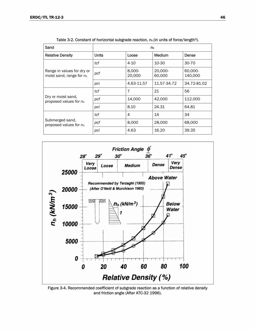
ERDC/ITL TR-12-3 46
Table 3-2. Constant of horizontal subgrade reaction, nh (in units of force/length3).
Sand nh
Relative Density Units Loose Medium Dense
Range in values for dry or moist sand, range for nh
tcf 4-10 10-30 30-70
pcf 8,000-20,000
20,000-60,000
60,000-140,000
pci 4.63-11.57 11.57-34.72 34.72-81.02
Dry or moist sand, proposed values for nh
tcf 7 21 56
pcf 14,000 42,000 112,000
pci 8.10 24.31 64.81
Submerged sand, proposed values for nh
tcf 4 14 34
pcf 8,000 28,000 68,000
pci 4.63 16.20 39.35
Figure 3-4. Recommended coefficient of subgrade reaction as a function of relative density
and friction angle (After ATC-32 1996).

ERDC/ITL TR-12-3 47
Assuming the soil is a well-graded medium dense sand with a relative density of 50 percent/and referring to Table 8 of FHWA-RD-97-130, Design Manual for Ground Anchor Walls, one would expect a moist unit weight of 118 pcf and an angle of internal friction of 34 degrees. The buoyant unit weight of the submerged sand is obtained by subtracting from its dry weight a quantity equal to its displaced volume. Assuming 30 percent voids; the buoyant unit weight of the submerged sand is approximately equal to 118 – [(100 – 30) / 100) x 62.4] or 74.3 pcf.
The proposed constant of horizontal subgrade reaction from Table 3-2 would be 21 pci for dry or moist sand and 16.2 pci for submerged sand.
Referring to Figure 3-4: For a relative density of 50 percent the constant of subgrade reaction is 3500 kN/m3 (12.89 pci) for a submerged sand and 5800 kN/m3 (21.37 pci) for a dry or moist sand, producing a wet to dry coefficient of subgrade reaction ratio of 0.60. The ratio of buoyant unit weight of submerged sand to moist unit weight is 74.3/118 = 0.63. This confirms that the lower constant of horizontal subgrade reaction for submerged sand is due to the lower confining pressure exerted by submerged sand.
The pushover analyses presented in Appendices A and B compare results for both submerged (wet) and dry sites recognizing that with respect pile bents subjected to barge impact submerged site conditions will always prevail.
The preliminary depth of embedment of the “long” vertical pile is deter-mined from the relative stiffness factor equations
/R EI k= 4 (3.5)
for a constant k (i.e., independent of depth), which would be found in clays and rock, and
/ (3.6)
for k = nhx (where the “stiffness” increases with increasing confining pressure with depth) in sands. Figure 3-5 shows these equations and their relationship with the embedded depth of the pile, as per the discussions by Davisson (1970).
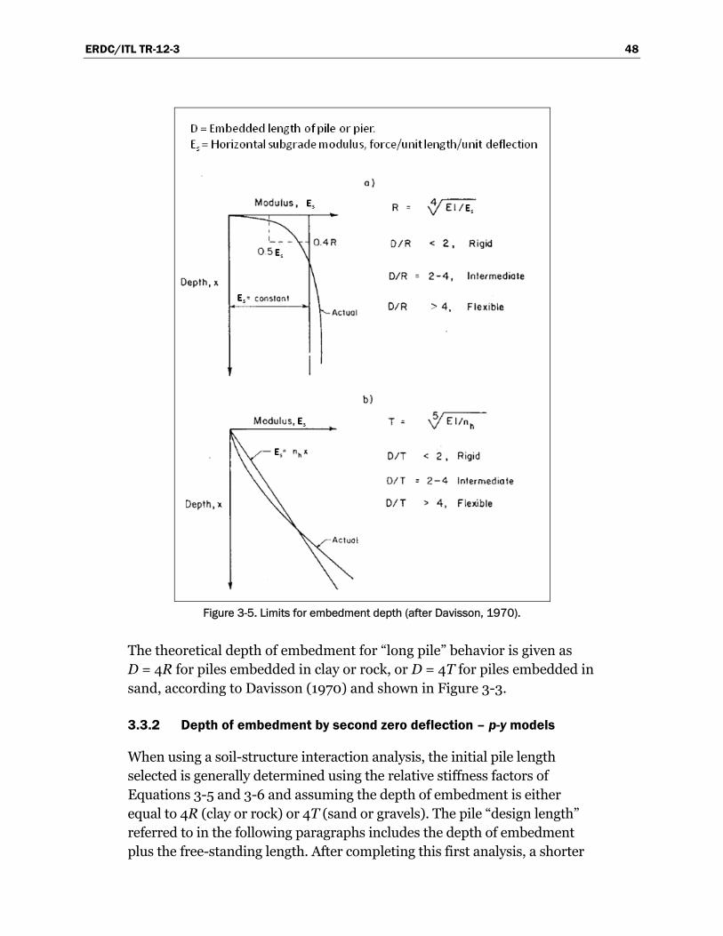
ERDC/ITL TR-12-3 48
Figure 3-5. Limits for embedment depth (after Davisson, 1970).
The theoretical depth of embedment for “long pile” behavior is given as D = 4R for piles embedded in clay or rock, or D = 4T for piles embedded in sand, according to Davisson (1970) and shown in Figure 3-3.
3.3.2 Depth of embedment by second zero deflection – p-y models
When using a soil-structure interaction analysis, the initial pile length selected is generally determined using the relative stiffness factors of Equations 3-5 and 3-6 and assuming the depth of embedment is either equal to 4R (clay or rock) or 4T (sand or gravels). The pile “design length” referred to in the following paragraphs includes the depth of embedment plus the free-standing length. After completing this first analysis, a shorter

ERDC/ITL TR-12-3 49
“design length” is established. This is done either by using the greater design length required for axial load support, or by using one of the three Lien (2011) methods described and illustrated subsequently. The final “design length” chosen makes use of a point along the pile that is referred to by Lien (2011) as the Point of Fixity (POF). It should be recognized however that the Lien (2011) POF differs with respect to the “depth to fixity” used in structural design to obtain an equivalent analytical model where the deflection and rotation at the top of the fixed base equivalent pile as well as the critical buckling load are the same as for the actual pile. As Lien (2011) points out, there is no universal agreement on how to define the POF needed to achieve long pile behavior. However, it is clear that the Lien (2011) POF, defined as the minimum design length required for long pile behavior, will be greater than the depth to fixity described in Figure 3-9b and labeled “Fixed Base Equivalent”.
Lien (2011) has cited eleven separate definitions for Point of Fixity (POF) and thus several methods for determining the design length, i.e., minimum length of pile that is required below the impact deck. In an assessment made by Lien (2011), it was concluded that three of these are potential candidates for determining design pile length for layered soil systems where a soil-structure interaction analysis (such as COM624G, CBEAMC, or LPILE) has been used for the analysis. The methods require that the designer review the displacement output for each pile increment and select the particular pile location as defined by one of the three figures provided below.
The first of three methods recommended by Lien (2011) for determining the design length is described and illustrated in Figure 3-6. It uses the deflected shape of the pile under service load conditions for establishing the design length based on the second zero deflection point.
Greater design lengths may result from greater impact loads, since with increased load there can be a greater number of p-y curves reaching their passive limit state capacities thereby requiring embedment to be deepened to achieve stability, or in the case of CBEAMC, a deeper embedment to obtain solution convergence. Since extreme barge impact loads are greater than usual or unusual loads (refer to Table 1-1), the extreme loading condition will be that controlling minimum pile design length and depth of embedment. This is the case for all three methods recommended by Lien (2011).
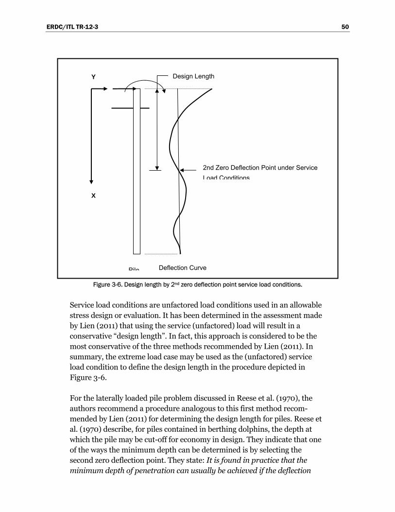
ERDC/ITL TR-12-3 50
Figure 3-6. Design length by 2nd zero deflection point service load conditions.
Service load conditions are unfactored load conditions used in an allowable stress design or evaluation. It has been determined in the assessment made by Lien (2011) that using the service (unfactored) load will result in a conservative “design length”. In fact, this approach is considered to be the most conservative of the three methods recommended by Lien (2011). In summary, the extreme load case may be used as the (unfactored) service load condition to define the design length in the procedure depicted in Figure 3-6.
For the laterally loaded pile problem discussed in Reese et al. (1970), the authors recommend a procedure analogous to this first method recom-mended by Lien (2011) for determining the design length for piles. Reese et al. (1970) describe, for piles contained in berthing dolphins, the depth at which the pile may be cut-off for economy in design. They indicate that one of the ways the minimum depth can be determined is by selecting the second zero deflection point. They state: It is found in practice that the minimum depth of penetration can usually be achieved if the deflection
Y
X
Pile Deflection Curve
2nd Zero Deflection Point under Service
Load Conditions
Design Length

ERDC/ITL TR-12-3 51
diagram under load corresponding to the design energy crosses the zero deflection point at least twice.
3.3.3 Depth of embedment by maximum negative deflection – p-y models
The second of three methods recommended by Lien (2011) for determining the design length is described and illustrated in Figure 3-7. The design length, the length to POF, is to the point along the pile possessing the maximum negative deflection. Like the previous method (depicted in Figure 3-6), this method utilizes the deflected shape of the pile but differs in that the deflected shape is computed using factored loads rather than service (unfactored) loads. Load factor information with respect to extreme barge impact events is provided in Section 1.9 of Chapter 1. It has been determined in the assessment made by Lien (2011) that this approach will provide a conservative “design length”.
Figure 3-7.Design length by maximum negative deflection point factored loads and strength
design.

ERDC/ITL TR-12-3 52
According to Lien (2011), this method (shown in Figure 3-7) for deter-mining the design length seems to be the most suitable because; (1) it is considered to be conservative, and (2) because it is based on “factored” rather than “service” loads. He states that this approach is used by the North Carolina Department of Transportation (NCDOT). It is important to observe that determining the design length by maximum negative deflection is not as conservative as basing it on the second zero deflection point (see Figure 3-6).
3.3.4 Depth of embedment by iteration – p-y models
The last of the three methods recommended by Lien (2011) for determining the design length is illustrated using Figure 3-8. In this method, the design length lies somewhere between the first zero deflection point and the maxi-mum negative deflection point. This method requires several iterations to develop a pile length vs. pile deflection plot. This approach would be possible if COM624G or LPILE were used for the analysis. It would not be possible with CBEAMC (Dawkins 1994) because the program may be unable to converge on a solution for the shorter pile lengths. The method provides a depth of penetration representing the onset of “long pile” behavior. Referring to Figure 3-8, the procedure is as follows:
An initial “trial pile length” of 16 ft is assumed and a simplified SSI analysis is conducted (e.g., using COM624G). The lateral displacement at the top of pile is computed and recorded, as shown in the right insert figure.
The assumed “trial pile length” is extended to 17 ft and the lateral displacement at the top of pile is computed and recorded in Figure 3-8.
The “trial pile length” is extended in subsequent analyses with the displacement results recorded in the right insert figure.
The minimum “design length” is set equal to “trial pile length” at which the top of pile displacements start increasing at a faster rate for reduction in pile length; 22 ft in this problem.
The “design length” would be set equal to the 22-ft depth identified in this figure. When applying this procedure, it is important to check that the computed depth length is greater than the first zero deflection cross-over point. Like the previous method (depicted in Figure 3-7), this method utilizes the deflected shape of the pile. The deflected shape is computed using factored loads (rather than service unfactored loads).
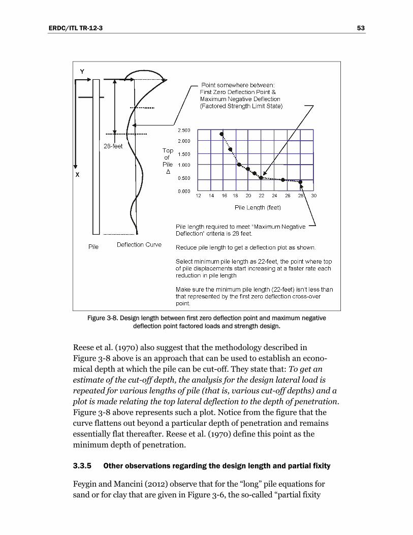
ERDC/ITL TR-12-3 53
Figure 3-8. Design length between first zero deflection point and maximum negative
deflection point factored loads and strength design.
Reese et al. (1970) also suggest that the methodology described in Figure 3-8 above is an approach that can be used to establish an econo-mical depth at which the pile can be cut-off. They state that: To get an estimate of the cut-off depth, the analysis for the design lateral load is repeated for various lengths of pile (that is, various cut-off depths) and a plot is made relating the top lateral deflection to the depth of penetration. Figure 3-8 above represents such a plot. Notice from the figure that the curve flattens out beyond a particular depth of penetration and remains essentially flat thereafter. Reese et al. (1970) define this point as the minimum depth of penetration.
3.3.5 Other observations regarding the design length and partial fixity
Feygin and Mancini (2012) observe that for the “long” pile equations for sand or for clay that are given in Figure 3-6, the so-called “partial fixity

ERDC/ITL TR-12-3 54
point” is the first zero-deflection point along the pile embedment length that has developed at least two zero-slope points. This “partial fixity point” (located at the depth Lf in Figure 3-91) can be described by a rotational spring, given by Equation 3.7. They further observe that some traditional designs based on full-fixity at the zero-deflection point greatly under-estimate flexural movement at the pile-to-pile cap interface and is a likely reason for failures during extreme seismic events.
Figure 3-9. Davisson fixed base equivalent that retains “long pile” behavior at top
of pile (after Davisson, 1970).
Feygin and Mancini (2012) endorse Tsinker’s (2004) suggestion of another model utilizing non-linear springs (i.e., P-y nonlinear curves) for pile-soil supports in finite element software packages; and that these non-linear supports predict forces at the pile-to-cap interface better. They observe that linear Winkler springs, traditionally used for pile bent analysis, have a tendency to place the zero-deflection point significantly higher on the piles, underestimating soil crushing. It is also recognized that the use of non-linear soil springs increases the complexity of the pile bent analysis.
1 Lf is shown in Figure 3-9 and calculated using Equation 3-8 or Equation 3-9 for a clay site and sand
site, respectively.

ERDC/ITL TR-12-3 55
Current design practice according to Gaythwaite (2004) use analytical models developed by Davisson (1970) that assume piles in a pile bent have a depth to fixity some distance Lf below the mud-line and assume that this depth to fixity plus the free-standing length are equal to half the critical buckling length. Gaythwaite emphasized that this approach only applies when the total pile embedment exceeds three times Lf. Feygin and Mancini (2012) state that Gaythwaite was only partially correct and that what Gaythwaite has identified is nothing more than the zero-deflection point whose partial fixity is represented by a rotational spring with stiffness defined as:
Θr
Mk = (3.7)
where:
M is the flexural moment at zero-deflection point, and is the slope of the elastic curve at zero-deflection point.
Feygin and Mancini (2012) also state that:
To produce a partial fixity condition, the pile embedment length should be sufficient to develop at least two zero-slope points within the soil medium.
The Gaythwaite (2004) “arbitrary” requirement that the total pile embedment length exceed three times Lf sometimes falls short of the requirement posited in their first statement.
Subsequently discussed in Subsection 3.4.1, the depth of fixity (Lf) recom-mended by Davisson (1970) to obtain an equivalent structural analytical model (where the deflection and rotation at the top of the fixed base equivalent pile as well as the critical buckling load are the same as for the actual pile) is equal to 1.4R for clays and 1.8T for sands. The Gaythwaite (2004) requirement that the total pile embedment length exceed three times Lf gives a minimum depth of embedment for vertical piles equal to 4.2R for clays and 5.2T for sands which is greater than the Davisson (1970) Figure 3-5 “long pile” behavior guidance of 4R for clays or 4T for sands. Feygin and Mancini’s (2012) comments about Gaythwaite above imply that the Davisson guidance is unconservative, also.

ERDC/ITL TR-12-3 56
The Davisson (1970) “long pile” guidance is used by many engineers to establish a minimum depth of embedment for vertical piles subjected to lateral loading. Considering the expense for placement of a pile foundation, additional research into guidance for minimum depth of embedment criteria (for vertical piles) is warranted.
3.4 Equivalent depth to fixity for analytical models
In engineering practice there are methods where a simple “depth to fixity” analytical model can be used to approximate the behavior of partially embedded piles. Three of these methods; Davisson (1970), Budeket al. (2000) and Yang (1966) are described in the following paragraphs.
3.4.1 Davisson (1970) equivalent free standing pile
For those problems in which the computation of maximum moments is the only concern, Davisson (1970) suggests that maximum moments can be approximated by modeling a portion of the pile with the embedded length (Lf) fixed at the depth as illustrated in Figure 3-9.
If k = constant and (Lu/R)>2, then Lf = 1.4R, or (3.8)
If k = nh x and (Lu/T)>1, then Lf = 1.8T (3.9)
The Davisson fixed model solution (i.e., the fixed base equivalent in Figure 3-6b) satisfies the conditions that the deflection and rotation at the top of the equivalent pile as well as the critical buckling load are the same as for the complete, non-fixed pile of Figure 3-6a.
3.4.2 Budeket al. (2000) analytical model
Budek et al. (2000) researched the topic of seismic response of drilled-shaft columns in sand, using finite elements to model the pile. As a result of this research, recommendations were made for the depth of fixity required in their analytical model to obtain results representative of long pile behavior. The models that they were working with were a free and a fixed head sys-tem, as shown in Figure 3-10. This figure also shows the differing distribu-tion of moments along a pile for a free head versus fixed head pile system. The results showed that the controlling hinge forms at the pile-cap connec-tion for a fixed head pile because the moments peak there. A second, sub-grade hinge usually results when the fixed head pile attains its full inelastic potential.

ERDC/ITL TR-12-3 57
Figure 3-10. Moment patterns in free and fixed head piles.
For these systems, the pile shaft length selected for the analytical model was the pile shaft length required to simulate “long” pile behavior. A six-ft diameter drilled-shaft was the basis for their model studies. According to Budek et.al. (2000), “long” pile behavior results when further lengthening of the pile will not reduce lateral displacement at yield.
The Budek et al. (2000) method of analysis uses a Winkler beam sand-to-pile model which is consistent with the method employed by COM624G (Figure 3-11). The Winkler beam model models a pile as a cantilever beam fixed against translation and rotation at the point of effective fixity and supported by sand-to-pile springs with a stiffness that models the soil behavior. For sand possessing a constant value for subgrade reaction modulus nh and a node’s tributary length Li (between vertical pile nodes), there is a linear increase in “stiffness” with depth (x) by the relationship
i i i hk x L n= (3.10)
The depth of the pile end is chosen by Budek et al. (2000) for “pile” behavior where the end displacement is less than 0.001 times the head displacement. This end depth can be determined from Figures 3-12 and 3-13 for free and fixed pile head boundary conditions, respectively. The plots show depth versus nondimensional system stiffness, given by:
*h
e
n d
d EI
6
(3.11)

ERDC/ITL TR-12-3 58
Figure 3-11. Winkler beam model of soil-to-pile substructure
(d=pile diameter) (after Budek et al. 2000).
Figure 3-12. Equivalent depth to fixity, free-head pile in sand (After Budek et al. 2000).

ERDC/ITL TR-12-3 59
Figure 3-13. Equivalent depth to fixity, fixed-head pile in sand (After Budek et al., 2000).
where nh is the subgrade reaction modulus of the sand, d is the pile diameter, d* is the “base” pile diameter of six ft, and EIe is the effective cracked-section stiffness for the reinforced concrete pile (Budek et al. 2000 refers to Ie as Ieff) . The vertical axis in these two figures report the depth to fixity as a multiple of pile diameter. The equivalent depth of fixity will be greater than 2.5 but less than 6 times the pile diameter d, and depends on the value for the nondimensional system stiffness.1
Recall that Figures 3-12 and 3-13 were developed from a six ft diameter drilled-shaft column SSI modeling and analysis effort. Budek et al. (2000) did not provide guidance on the applicability of these diagrams to other types of piles, e.g., H-piles or pipe piles.
3.4.3 Yang (1966) equivalent free standing pile
Yang (1996) uses the solution for the buckling strength of piles with variable subgrade reaction as proposed by Davisson (1963) to obtain a depth to fixity analytical model for application in the design of partially embedded piles.
The Yang (1966) methodology has been incorporated as input into the analysis using the Corps CPGA computer program. This combined method is used as the basis for the pushover examples of Appendices A and B. It has 1 This follows the form of Equation 2.3, but using nh rather than K for this sand site.

ERDC/ITL TR-12-3 60
the advantage over the other analytical models that the buckling capacity of piling and various levels of pile head displacement demand can be deter-mined. As with Davisson (1970) the depth to fixity is a function of the relative stiffness factor T, but also takes into account the free-standing length, as well as pinned-head nontranslating, pinned-head translating, fixed-head nontranslating, and fixed-head translating conditions. The Yang (1966) method is described in detail in subsequent paragraphs of this Chapter.
3.5 Effective stiffness – drilled in place piles
The material contained in this section was first presented in Strom and Ebeling (2005), which states that the effective stiffness of structural systems consisting of reinforced concrete drilled in place piles under yield conditions can be significantly less than that represented by gross section properties.
To obtain a best estimate of force and displacement demands on reinforced concrete members, the cracked section (i.e., effective) stiffness rather than the gross stiffness is often used for those members. The effective stiffness is an average value for the entire member and considers the distribution of cracking along the member length. The effective stiffness of reinforced concrete structures can be estimated based on the relationship between the cracking moment (i.e., the moment required to initiate cracking while ignoring the reinforcing steel) and the nominal moment capacity of the reinforced concrete section. For fixed head piles, these regions will be where the pile intersects the top of bent, as well as just below the “mud” line (i.e., top of soil) when secondary “hinging” occurs. For free head piles, it will be just below the “mud” line. Once the cracking moment MCR and the nominal moment capacity MN have been determined, the ratio of the effective stiffness Ie to the gross stiffness IG can be estimated as follows:
. .e N
G CR
I M
I M
é ùê ú= - -ê úë û
0 8 0 9 1 (3.12)
The ratio of Ie/IG should not be greater than 0.8, nor less than 0.25, according to Priestley (1987) and presented in Appendix G of Strom and Ebeling (2005).
This equation is a simplified version of American Concrete Institute (ACI) (2002) 318-02 equations commonly used for the deflection evaluation of
ERDC/ITL TR-12-3 61
reinforced concrete structures. The basis for the simplified version is contained in Priestly (1997) and also discussed in Moehle (1997) (which is presented in Appendix G of Strom and Ebeling, 2005) with respect to lightly reinforced concrete structures.
The nominal moment strength can be determined in accordance with standard ACI 318-02 (2002) procedures. The cracking moment MCR can be determined by equating the maximum tensile stress in a member (gross section) subjected to an axial load and the bending moment to the modulus of rupture as defined by ACI 318-02 (2002).
This process results in the following expression:
CR r b
PM f S
A
æ ö÷ç= + ÷ç ÷çè ø (3.13)
where:
fr = modulus of rupture = 7.5 (psi units) P = axial load A = area Sb = section modulus
It is the relative stiffness as defined by Equations 3-5 and 3-6 that is important to the pushover analysis; and for this reason it is recommended that, as a reasonable approximation, an Ie/IG ratio equal to 0.5 should be used for depth to fixity and embedment depth calculations.
3.6 Pushover analysis of drilled-in-pile bents
This chapter summarizes the pushover analysis procedure as it applies to drilled-in-pile (DIP) bent systems. As stated previously, the pushover analysis is a step-by-step procedure using superposition. The structure is laterally distorted to some limiting capacity value, frozen in that position, local yielding elements are relaxed, and the structure is laterally distorted to the next limiting capacity value. The procedure is repeated until the structure has reached a limit state consistent with an established performance objective.

ERDC/ITL TR-12-3 62
3.7 DIP bent system
In the drilled-in pile system (Figure 3-14), flexural yielding mechanisms take place at the caisson to reinforced concrete cap connection followed by yielding at the point of moment fixity below the mud line. A key aspect of this type of deformable approach wall, with regard to the analysis procedures being used in this section, is that all piles are vertical, i.e., without batter.
Figure 3-14. DIP bent flexural yielding.
To account for soil-pile interaction effects below the mudline the pushover analysis can be performed by one of the following three methods:

ERDC/ITL TR-12-3 63
Yang (1966) approach Saul (1968) approach Nonlinear p-y curve approach
3.7.1 Pushover analysis using Yang (1966) approach
This method is based on a coefficient of subgrade reaction approach in which the stiffness of the sand varies linearly with depth. A relative stiffness factor T for a drilled in place pile is calculated by the following:
c e
h
E IT
n= 5 (3.14)
where:
Ec = the modulus of elasticity of concrete used for drilled-in caisson;
Ie = the effective moment of inertia of the drilled-in caisson; nh = the coefficient of subgrade reaction for the sand.
In all the pushover analyses for drilled-in caissons, a constant effective moment of inertia Ie is used to develop the load-deflection response. The effective moment of inertia Ie may be for a section that has cracked. This is a simplification that is conservative with respect to potential energy capacity.
In the Yang (1966) approach a coefficient of free standing length m is used to estimate moments at the fixed-head and below the mudline:
oLm
T= (3.15)
where:
Lo = the free standing length of the pile above the mudline.
With a known value for the coefficient of free standing length m and assuming a fixed-head condition, Yang (Figure 2, 1966) reports that a coefficient of effective embedment, designated a in Figure 3-15, and total length (Lo + aT) from top of pile to the point of effective embedment can

ERDC/ITL TR-12-3 64
be determined1. The first increment of horizontal force that brings the pile moment at the cap to ultimate can be estimated as:
Figure 3-15. Effective embedment of pile (after Figure 2 Yang,
1966).
( )
UTH
O
MP
L aT=
+1
2 (3.16)
where:
MUT = ultimate moment capacity at top of pile.
According to Yang (Figure 7, 1966) and assuming a fixed top condition, the coefficient of horizontal load H1 can be selected from Figure 3-16 and the moment demand (MB) below the mudline determined by:
1 The effective embedment length of Figure 3-15 term a times the Equation 3-14 T value is referred to as
the “depth of fixity” in this report. Observe in Figure 3-15 that the depth of fixity (i.e., a times T) is a function of both the free standing length and the boundary condition at the pile cap. Recall that the Davisson’s (1970) depth of fixity relationships for Lf are independent of these two factors. Figure 3-15 indicates that these factors are important considerations for estimating the depth of fixity.
Coefficient of free standing length (m)
Coef
ficie
nt o
f eff
ectiv
e em
bedm
ent (
a)

ERDC/ITL TR-12-3 65
Figure 3-16. Coefficient of horizontal load capacity (Figure 7, after
Yang 1966).
[ ]
HB
P TM
H= 1
1
(3.17)
and the reserve moment capacity below the mudline (MBR) determined by:
BR UT BM M M= - (3.18)
The second increment of horizontal force PH2 that brings the pile moment below the mudline to ultimate can be estimated by assuming a pinned top condition and using Figure 3-15 to select a the coefficient of horizontal load H2, then performing the following calculation.
[ ]BR
H
M HP
T= 2
2 (3.19)
Coefficient of free standing length (m)
Coef
ficie
nt o
f hor
izon
tal l
oad
(H)

ERDC/ITL TR-12-3 66
According to Yang (Figure 8, 1966), assuming a fixed top condition, and using Figure 3-17 to select a coefficient of horizontal deflection D1, the displacement (y1) associated with hinging at the pile cap due to the first increment of loading PH1 can be determined by:
Figure 3-17. Coefficient of horizontal deflection (after Figure 8 Yang,
1966).
[ ]H
c e
P Ty D
E I=
31
1 1 (3.20)
By assuming a pinned top condition and using Figure 3-17 to select a coefficient of horizontal deflection D2, the displacement y2 associated with hinging below the mudline due to the second increment of loading PH2 can be determined by:
[ ]H
c e
P Ty D
E I=
32
2 2 (3.21)
The pushover process, using the graphical solution procedures proposed by Yang (1966), is illustrated in Figure 3-18.
Coefficient of free standing length (m)
Coef
ficie
nt o
f hor
izon
tal d
efle
ctio
n (D
)

ERDC/ITL TR-12-3 67
Figure 3-18. Fixed-head bent system analysis by Yang (1966) method.
3.7.2 Pushover analysis using Saul (1968) approach
Saul (1968) suggested an engineering approach for which a rigid pile cap is assumed and the stiffness of each pile determined for either a pinned head condition or fixed-head condition based on a supporting soil that is represented as Winkler springs with a stiffness that is either constant with depth (cohesive soils) or varies linearly with depth (granular soils). The stiffness coefficients of all piles are summed to determine a stiffness matrix for the pile group. The stiffness matrix considers axial load effects as well as lateral load effects. The Saul (1968) analysis approach can be accomplished using the Corps CPGA computer program. For a fixed-head pile bent system

ERDC/ITL TR-12-3 68
the piles would first be considered as fixed. The pile group would be laterally loaded, incrementally, until the horizontal force creates a moment equal to the ultimate moment capacity of the pile at the pile head. The displacement associated with this action is provided by the CPGA program as well as the maximum moment demand below the mudline. The reserve moment capacity of the pile below the mudline is determined. The piles are then modeled as pinned (moment at the pile head released) and the incremental lateral loading of the pile is resumed until the horizontal force creates a moment equal to the reserve moment capacity. The forces and displacements associated with each of the two load increments is then used to develop a load-displacement curve. The Saul (1968) pushover analysis process is illustrated in Figure 3-19.
Figure 3-19. Fixed-head bent system analysis by Saul (1968) method 3.7.3 nonlinear p-y curve approach.

ERDC/ITL TR-12-3 69
A nonlinear p-y curve approach can also be used to evaluate the load displacement response of a fixed-head bent system. This can be accomp-lished using the Corps COM624G computer software. This software is limited to the response of a single laterally loaded pile. With a rigid cap, it can be assumed that each pile responds the same and as such a COM624G analysis is suitable. In COM624G the soil response is nonlinear; therefore, it is necessary to capture the response from the first load increment before starting the second load increment. The nonlinear response that occurs during the first load increment would be lost if the second increment of loading were started from a no-load condition. The first increment assumes fixed-head conditions until the moments at the top of pile have reached the ultimate moment capacity. This occurs when the moment demands at the pile cap, as observed from the COM624G analysis, are equal to the moment capacity as determined by an axial load – moment interaction analysis of the types described in Chapter 2. The second increment, to accommodate the nonlinear response of the soil, assumes a free-head condition and applies a moment equal to the ultimate moment capacity of the pile at the cap. This is accomplished in the COM624G analysis by using a free head boundary condition and specifying a moment equal to the moment capacity at the top of the pile. With the cap moment locked in, the pile lateral load is increased until the moment capacity of the pile below the mudline is reached. Using the force and displacements obtained from the COM624G analysis a load-displacement curve can be developed. The nonlinear p-y curve pushover analysis process is illustrated in Figure 3-20.
3.8 Results from pushover analysis
For the pushover analyses presented in Appendix A, the total length of the pile specified was 100 ft, with 40 ft being the unembedded length and 60 ft being the embedded length. Because this embedded length is longer than 39.4 ft for the dry site1 and longer than 44.8 ft for the wet site2, long pile behavior is accurately modeled.
Load displacement plots for all three methods as presented in Appendix A are summarized in Figure 3-21. The load displacement plots are for a single pile of a two-pile bent. The single pile approach is employed to accommo-date the limitations of Yang (1966) and COM624G which only accommo-date a single pile analysis approach. When using the single pile approach,
1 Referring to Section A-4 in Appendix A for the dry site; D = 4T = 4 times 9.85 feet = 39.4 feet. 2 Referring to Section A-7 in Appendix A for the wet site; D = 4T = 4 times 11.2 feet = 44.8 feet.

ERDC/ITL TR-12-3 70
for fixed-head conditions, it is assumed that rotation at the pile cap is prevented; and for a free-head condition, it is assumed that rotation for both piles is unrestrained and equal. These assumptions, although approximate, are commonly used in the design/evaluation of bridge bents. The load-displacement results for a two pile bent will have similar displacement points, but the two-pile bent loads will be twice those for a single pile. Likewise the potential energy capacity will be twice that for a single pile.
Figure 3-20. Fixed-head bent system analysis by nonlinear p-y curve (COM624G) analysis.
Fixed-Head
Two-pile bent system
Push single pile of two-pile fixed-head bent system
∆
Increment 1 Model boundary conditions at cap for a specified lateral load and a specified slope at pile head (slope = 0). Increase lateral load incrementally until the ultimate moment capacity of the pile at the pile cap is reached. Record load increments and displacements.
Increment 2 Model boundary conditions at cap as free head and specify moment at cap as the ultimate moment capacity. Increase lateral load incrementally until the ultimate moment capacity of the pile below the mudline is reached. Record load increments and displacements.
Ultimate moment capacity of pile at cap
Ultimate moment capacity of pile below mudline
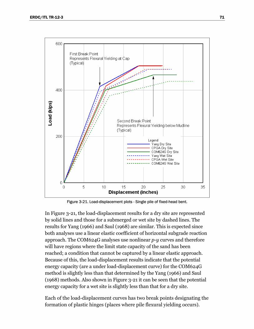
ERDC/ITL TR-12-3 71
Figure 3-21. Load-displacement plots - Single pile of fixed-head bent.
In Figure 3-21, the load-displacement results for a dry site are represented by solid lines and those for a submerged or wet site by dashed lines. The results for Yang (1966) and Saul (1968) are similar. This is expected since both analyses use a linear elastic coefficient of horizontal subgrade reaction approach. The COM624G analyses use nonlinear p-y curves and therefore will have regions where the limit state capacity of the sand has been reached; a condition that cannot be captured by a linear elastic approach. Because of this, the load-displacement results indicate that the potential energy capacity (are a under load-displacement curve) for the COM624G method is slightly less than that determined by the Yang (1966) and Saul (1968) methods. Also shown in Figure 3-21 it can be seen that the potential energy capacity for a wet site is slightly less than that for a dry site.
Each of the load-displacement curves has two break points designating the formation of plastic hinges (places where pile flexural yielding occurs).

ERDC/ITL TR-12-3 72
The first break point (with lowest displacement demand) occurs when flexural yielding takes place at the pile to pile cap connection. The second break point occurs when flexural yielding takes place at the point of maximum moment below the mudline.
The termination of the load displacement curve occurs when the rotation of the pile in the plastic hinge region below the mudline has reached its ultimate rotational capacity. This is illustrated by calculations contained in Appendix A.
3.9 Pile interaction effects
When piles are placed in close proximity to each other, the effects of the pile interacting with the embedding soil can be propagated to nearby piles. This affects the stiffness of the entire pile group. Davisson (1970) alluded to this, and provided “rule of thumb” guidelines for establishing the stiffness of a pile system according to the distance between piles (for both in-line piles and side-by-side piles, as defined by the direction of loading), as shown in Figure 3-22. He did not cite studies or provide calculations supporting these guidelines.
Figure 3-22. Limits for interaction between piles in a pile group.
Experimental studies conducted by Prakash (1962), Cox et al. (1984), Wang and Reese (1986), and Lieng (1988) have included loading tests on side-by-side piles with loading applied perpendicular to the line of piling. Reese et
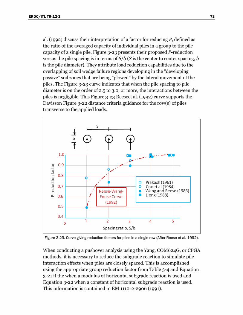
ERDC/ITL TR-12-3 73
al. (1992) discuss their interpretation of a factor for reducing P, defined as the ratio of the averaged capacity of individual piles in a group to the pile capacity of a single pile. Figure 3-23 presents their proposed P-reduction versus the pile spacing is in terms of S/b (S is the center to center spacing, b is the pile diameter). They attribute load reduction capabilities due to the overlapping of soil wedge failure regions developing in the “developing passive” soil zones that are being “plowed” by the lateral movement of the piles. The Figure 3-23 curve indicates that when the pile spacing to pile diameter is on the order of 2.5 to 3.0, or more, the interactions between the piles is negligible. This Figure 3-23 Reeseet al. (1992) curve supports the Davisson Figure 3-22 distance criteria guidance for the row(s) of piles transverse to the applied loads.
Figure 3-23. Curve giving reduction factors for piles in a single row (After Reese et al. 1992).
When conducting a pushover analysis using the Yang, COM624G, or CPGA methods, it is necessary to reduce the subgrade reaction to simulate pile interaction effects when piles are closely spaced. This is accomplished using the appropriate group reduction factor from Table 3-4 and Equation 3-21 if the when a modulus of horizontal subgrade reaction is used and Equation 3-22 when a constant of horizontal subgrade reaction is used. This information is contained in EM 1110-2-2906 (1991).

ERDC/ITL TR-12-3 74
Table 3-4. Laterally loaded pile group reduction factors, Rg (after EM 1110-2-2906).
Center-Line-to-Center-Line Pile Spacing in Direction of Loading (d=pile diameter) Group Reduction Factor Rg
3d 3.0
4d 2.6
5d 2.2
6d 1.8
7d 1.4
8d 1.0
For soils with a linearly increasing modulus of horizontal subgrade reaction, the following equation applies:
group
hh
g
nn
R= (3.22)
For soils with a constant modulus of horizontal subgrade reaction, the following equation applies:
group
ss
g
EE
R= (3.23)
3.10 Summary and conclusions
This chapter summarizes the various engineering procedures and corresponding software that may be used to conduct a pushover analysis of drilled-in-place pile bent systems. The focus of this effort is to compute the pushover capacity of a group of vertical (i.e., plumb) piles to obtain the load versus deformation relationship of the pile group. This load-deflection relationship is used with a balance of energy evaluation procedure to design a pile-founded flexible approach wall system for the usual, unusual and extreme barge train impact design load cases.
An important step in the design of groups of vertical piles subjected to lateral loading is determining the minimum required depth of embedment. The simplified procedure of Davisson (1970), that is summarized in Figure 3-3, as well as more rigorous procedures that make use of the computed results from non-linear SSI analyses (using nonlinear p-y soil-to-pile models) were discussed. The software COM624G is used in this latter
ERDC/ITL TR-12-3 75
category of SSI analysis. The authors of this report recommend that a non-linear SSI analyses be conducted when finalizing the minimum depth of embedment for the vertical piling contained within a pile group.
Three procedures have been outlined in this chapter for determining the depth of fixity for vertical piling. An example of the application of this depth of fixity in a simplified 3-D structural modeling effort for barge impact loading will be shown in Chapter 5. Three procedures for determining the depth of fixity were discussed; Davission’s (1970) Equations 3.8 and 3.9 for clay and sand sites, respectively (also see Figure 3-9b); Budek et al. (2000), Figures 3-12 and 3-13 for free-head and fixed-head, respectively, drilled-shaft columns in sand; and Yang’s (1966) Figure 3-15. Among these three procedures, the authors of this report recommend the use of Yang (1966).
3.11 Recommendations for further research
Considering the expense for placement of a pile foundation, additional research into guidance for minimum depth of embedment criteria is warranted. Specifically, further research is needed to determine which of the procedures discussed in Section 3.3 is best for interpreting the results nonlinear SSI analyses (e.g., using COM624G) to determine the minimum depth of embedment and to determine if the Davisson simplified relation-ships for minimum “long pile” behavior are adequate or unconservative.

ERDC/ITL TR-12-3 76
4 Pushover Analysis of Batter Pile Bent Systems
4.1 Pushover analysis approach
This chapter discusses the evaluation of batter pile bent systems using a pushover analysis.1 As with the Chapter 3 (and Appendix A) drilled-in-pile (DIP) system, the results of a pushover analysis of deformable approach walls are used to establish the capacity of the structural system to barge impact loadings. The pushover analysis for the batter-pile bent system is illustrated in Figure 4-1. The impact deck is supported on multiple rows of three-pile groups centered every six ft six in. along the deck. Each pile group consists of a row of three piles: Pile number one is vertical and piles number two and three possess a one horizontal to four vertical batter (i.e., a 3:12 slope).
Piling contained in a batter pile system must have sufficient strength to resist driving stresses. As a result, the axial capacity of the piling in either tension or compression is most often greater than the capacity of the soil. As the piles are loaded laterally the pile cap must move vertically as well as horizontally eventually causing sufficient tension in vertical piling (and possibly some batter piling) to cause some of the piles to pullout. Methods are described herein to improve the lateral load capacity of the system and the efficiency of the system.
Piles used in batter pile systems can be open end pipe piles, concrete-filled pipe piles, H-piles, or prestressed concrete piles. This system behaves differently from the drilled-in pile system (of vertical piles) because major yielding takes place as axial tension or axial compression, rather than flexure. The batter-pile bent system and its analytical model is illustrated in Figure 4-1.a. Without pile tip movement, the axial deformation due to pile compression or tension occurring between top of pile and the pile tip could be easily determined. However with pile tip movement, the pile axial stiffness must capture both axial deformations in the pile as well as tip movement due to pile-soil interaction.
1 Complete details of the pushover example problem discussed in this chapter are provided in Appendix B.

ERDC/ITL TR-12-3 77
Figure 4-1. Pushover for batter-pile bent system.
The Saul (1968) method (Computer Program CPGA) provides an excellent preliminary analysis tool for evaluation the load-displacement charac-teristics of batter-pile bent systems. Actual values for the axial stiffness modifier C33 used in CPGA for compression and tension piles should be determined by appropriate analytical models and pile load tests. However, simple assumptions with respect to stiffness modifiers can be used for preliminary load-displacement analyses. Assuming that the flexural response is insignificant, a first increment of lateral loading PH1 would be applied until the tensile capacity of the vertical pile or one of the batter piles is reached. Tensile capacity will be governed by skin-friction capacity. The skin friction capacity of a pile founded in sand may be determined using the procedures discussed in EM 1110-2-2906 (1991), including the methodology recommended by Mosher (1984), as presented in Appendix D.

ERDC/ITL TR-12-3 78
Once the axial tensile capacity of a tension pile is reached during the incremental load application in a pushover analysis, the pile is released for the second stage PH2 loading by introducing an axial stiffness modifier C33 that is negligible such that the pile will attract a negligible amount (nearly zero) of axial load during the second increment of loading.
Δ
Cδ
=33 (4.1)
where:
ΔPLAE
= (4.2)
The calculation of Δ assumes the pile is supported at its tip with all axial load P transferred to the tip and where:
δ = actual displacement of the pile under axial load P
During the second stage PH2 loading it is possible to reach and exceed:
The flexural capacity of the piles at the cap and below the mudline; The compressive capacity of piles as limited by foundation strengths; The buckling capacity of the piles.
During this stage, all three possible yield mechanisms must be monitored. Once a particular yield mechanism is identified the analytical model is altered by reducing member stiffness in a manner that simulates the yield mechanism. The new analytical model is then incrementally loaded and the process repeated until a collapse mechanism develops. As displacements from each increment accumulate, pile buckling becomes more likely. In general, the larger the top of pile lateral displacement the lower the bucking load.
The load increments and the associated failure mechanisms are indicated in a general manner in Figure 4-1b. The final load-displacement relationship is illustrated in a plot of the accumulation of load and displacement for each increment shown in Figure 4-1c. The area under the load-displacement response represents the energy absorbed, or potential energy capacity of the system.
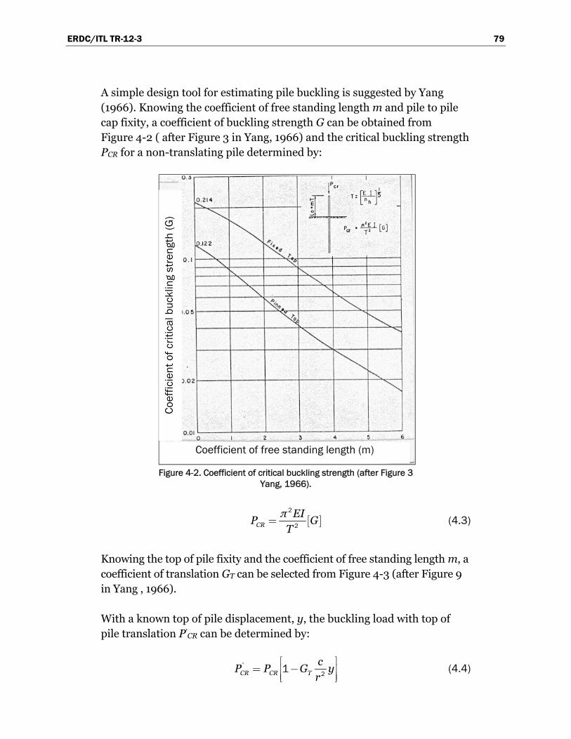
ERDC/ITL TR-12-3 79
A simple design tool for estimating pile buckling is suggested by Yang (1966). Knowing the coefficient of free standing length m and pile to pile cap fixity, a coefficient of buckling strength G can be obtained from Figure 4-2 ( after Figure 3 in Yang, 1966) and the critical buckling strength PCR for a non-translating pile determined by:
Figure 4-2. Coefficient of critical buckling strength (after Figure 3
Yang, 1966).
[ ]CR
π EIP G
T=
2
2 (4.3)
Knowing the top of pile fixity and the coefficient of free standing length m, a coefficient of translation GT can be selected from Figure 4-3 (after Figure 9 in Yang , 1966).
With a known top of pile displacement, y, the buckling load with top of pile translation P’CR can be determined by:
'CR CR T
cP P G y
r
é ù= -ê ú
ê úë û21 (4.4)
Coefficient of free standing length (m)
Coef
ficie
nt o
f crit
ical
buc
klin
g st
reng
th (G
)

ERDC/ITL TR-12-3 80
Figure 4-3. Coefficient decrement of buckling strength (after Figure 9
Yang, 1966).
where:
c = distance from pile neutral axis to extreme fiber; r = pile radius of gyration.
4.2 Pushover analysis summary
The pushover analysis is an approximate method for predicting deformation demands (elastic and inelastic) and for predicting the redistribution of internal forces occurring as yield mechanisms develop in response to incrementally applied barge impact loadings to a deformable approach wall. The method, though approximate, requires a reasonable characterization of the system and member force-displacement responses. For preliminary analysis this can be accomplished using simple force-displacement models. The resulting structural system versus displacement plot is illustrated in Figure 4-4 below. It characterizes the potential energy capacity of the particular batter pile bent being analyzed.
Load displacement plots for free-head and fixed-head bent systems analyzed in Appendix B are depicted in Figure 4-4.
Coefficient of free standing length (m)
Coef
ficie
nt o
f tra
nsla
ltion
(GT)
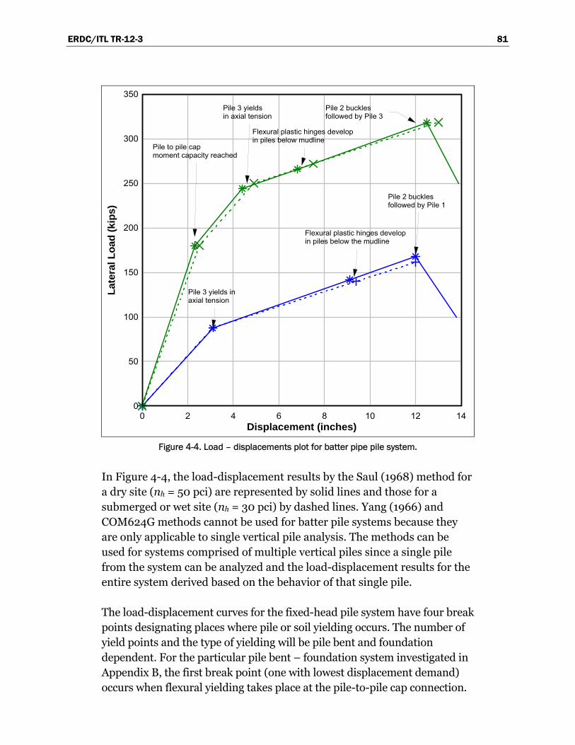
ERDC/ITL TR-12-3 81
Figure 4-4. Load – displacements plot for batter pipe pile system.
In Figure 4-4, the load-displacement results by the Saul (1968) method for a dry site (nh = 50 pci) are represented by solid lines and those for a submerged or wet site (nh = 30 pci) by dashed lines. Yang (1966) and COM624G methods cannot be used for batter pile systems because they are only applicable to single vertical pile analysis. The methods can be used for systems comprised of multiple vertical piles since a single pile from the system can be analyzed and the load-displacement results for the entire system derived based on the behavior of that single pile.
The load-displacement curves for the fixed-head pile system have four break points designating places where pile or soil yielding occurs. The number of yield points and the type of yielding will be pile bent and foundation dependent. For the particular pile bent – foundation system investigated in Appendix B, the first break point (one with lowest displacement demand) occurs when flexural yielding takes place at the pile-to-pile cap connection.
Displacement (inches)
Late
ral L
oad
(kip
s)
0 2 4 6 8 10 12 140
50
100
150
200
250
300
350
Pile to pile capmoment capacity reached
Pile 3 yields in axial tension
Flexural plastic hinges developin piles below mudline
Pile 2 bucklesfollowed by Pile 3
Pile 3 yields in axial tension
Flexural plastic hinges developin piles below the mudline
Pile 2 bucklesfollowed by Pile 1

ERDC/ITL TR-12-3 82
The second break point occurs when Pile number 3 yields in axial tension (a foundation to pile transfer mechanism).1 The third break point occurs when flexural yielding takes place in the piles below the mudline. The fourth break point occurs when Pile number 2 buckles. Pile buckling quickly results in pile bent system failure with little reserve potential energy capacity in the system.
There is little difference between the behaviors of submerged (wet) sites and dry sites, recognizing that lock approach wall bent systems will always be submerged. With batter pile systems, the resistance to lateral load comes principally from pile axial stiffness and not from flexural stiffness, as is the case with vertical pile systems. Therefore, changes in lateral subgrade resistance (e.g, nh) have little effect on system load-displacement behavior.
It can be recognized from Figure 4-4 that the fixed-head system has much greater potential energy capacity than the free-head system. The free-head system does not possess the added lateral force resistance provided by rigid pile-to-pile cap connections (which is the first break point for the fixed-head system).
An attempt was made to use the Group 7 software in a pushover analysis to develop a load-displacement response for the batter pile system of Appen-dix B. The Group 7 software permits various nonlinear actions to occur suggesting a more comprehensive load-displacement response was possible. The Group 7 analysis is presented in Appendix C. The computed displace-ment responses from Group 7 of the “dry” site closely mirrored those from CPGA for applied lateral loads greater than 80 kips and less than 140 kips. The Group 7 results show nonlinear force-displacement response for lateral loading less than 80 kips compared to linear response from the CPGA results, indicating that “softer” springs are being used at this lower load level in the CPGA push-over analysis. In this study, the Group 7 analyses did not provide critical insight on the formation of (failure) mechanisms as was indicated by results from the CPGA push-over analyses. The authors of this report speculate that this is a direct result of all nonlinear response features contained within the Group 7 analysis package. In addition, the Group 7 results for horizontal loading less than 80 kips indicate the soil springs in the CPGA analysis to be “soft”. The authors of this report therefore recommend the continued use of CPGA for pushover analyses.
1 Pile numbers are reported in Figure 4-1a.

ERDC/ITL TR-12-3 83
4.3 Batter pile system kinetic energy absorption efficiency
The batter pile system used herein to illustrate the pushover method was based on the system proposed for Lock and Dam 3 as illustrated in Appen-dix B. As a result of additional CPGA analyses, an alternative configuration of the pile groups was made, resulting in better pile group efficiency for the design barge impact loadings. A discussion of the procedure for improving pile group efficiency follows. Batter pile systems are rigid when compared to the vertical pile system described in Appendix A. This aspect of batter pile systems is discussed in Reese et al. (1970). The batter pile systems resists impact loads through a combination of axial thrust and flexural reaction in the piles. The lateral stiffness of the batter pile system is significantly increased due to the axial stiffness contribution of the batter piles. This leads to reduction in lateral displacement and a less-than-optimum response with respect to energy absorption.
As described previously, the first below grade yield mechanism for the Lock and Dam 3 batter pile system is likely to be caused by excess tension in Piles 1 or 3. Referring to Figure 4-5 below:
Figure Pile 1 will likely be in tension if the batter of the Pile 2-3 group is closer to vertical than the resultant of the applied loads;
Pile 3 will be in tension when the moment about the elastic center (R x DEC) causes an axial tensile force in the pile greater than its pure axial load compressive component (refer to equations in Figure 4-6).
It is unknown whether the tension in Pile 1 or the tension in Pile 3 will govern. This is problem dependent. The tensile loads in Piles 1 and 3 can be eliminated or reduced with a pile arrangement that is better suited to barge impact.
It is useful to use the elastic center method to see how axial performance can be improved. Figure 4-5 shows the Lock and Dam 3 bent system and its elastic center. Figure 4-6 provides the elastic center equations. Figure 4-7 provides the force diagram for the Lock and Dam 3 batter pile bent system and Figure 4-8 provides the force diagram assuming the batter was increased to 1 on 2.
As can be seen from the force diagram shown in Figure 4-7, Pile 1 will be in tension any time the barge impact load (BI) exceeds 25 percent of the dead load (DL) or at the point where the batter is steeper that the resultant (R).

ERDC/ITL TR-12-3 84
Figure 4-5. Elastic center for Lock and Dam 3 batter pile bent.

ERDC/ITL TR-12-3 85
Figure 4-6. Elastic center equations.
Figure 4-7. Force diagram for Lock and Dam 3 batter pile bent system.
1
4
DL
BI
R
Resultant compression in batter pile group (Group B) Resultant
tension in vertical pile (Group A)

ERDC/ITL TR-12-3 86
Figure 4-8. Force diagram for Lock and Dam 3 batter pile bent system with 2 on 1 batter.
By increasing the batter from 4 on 1 (i.e., a 3:12 slope) to 2 on 1 (i.e., a 6:12 slope) it can be seen from the force diagram shown in Figure 4-8 that Pile 1 is now in compression for the same barge impact (BI) load and tension in Pile 1 will not develop until the barge impact load (BI) exceeds 50 percent of the dead load (DL).
By rearranging the piles and increasing the batter (as shown in Figure 4-9), the problem related to axial tension can be reduced or eliminated. The piling foundations system consists of two alternating rows of pile groups; pile Group A consists of three vertical piles (labeled pile numbers 1, 2 and 3 in this figure) and pile Group B consists of three batter piles (labeled pile numbers 4, 5 and 6). Observe in Figure 4-9 that the batter of Group B has been increased to 1 horizontal to 2 vertical (i.e., 6:12 slope) from the Figure 4-1 batter of 1 horizontal to 4 vertical (i.e., 3:12 slope). The increased batter keeps the vertical piles in compression. The new pile arrangement places the load resultant close to the elastic center of the pile groups, as depicted in Figure 4-9. By keeping the load resultant close to the elastic center, an improvement in pile group efficiency is achieved with respect to linear elastic performance.
Performance characterized as linear elastic would fall within the range limited by the origin and Point A, as illustrated in Figure 4-10. Figure 4-10 depicts the response of the fixed-head bent system at a wet site as originally presented in Figure 4-4. Absorption of barge train kinetic energy (KE) in the nonlinear range is essential to meeting performance objectives associated

ERDC/ITL TR-12-3 87
Figure 4-9. Elastic center for Lock and Dam 3 batter pile bent alternative.
with extreme barge impact loadings. Performance characterized as non-linear includes the region from Point B to Point D in Figure 4-10. Efforts made to improve lateral load capacity in the linear elastic range (i.e., from the origin to Point A) may decrease KE absorption in the nonlinear range (i.e., from Point A to Point D). Increasing batter or the number of piles may cause certain yield mechanisms to occur at lower displacements, thereby leading to a decrease in total KE absorption.
It needs to be remembered that the absorption of barge train kinetic energy (KE) is key to meeting performance objectives described in Chapter 1. Therefore, pile group performance must be investigated with every change in configuration (i.e., batter, number of piles, pile arrangement) using a complete pushover analysis.
It should be noted that the Corps computer program CPGA provides elastic center information to help engineers evaluate the behavior and efficiency of a given pile group to a given barge impact loading. When developing pile group models of the types shown in Figure 4-9, pairs of

ERDC/ITL TR-12-3 88
Figure 4-10. Load – displacements plot for batter pipe pile system indicating regions of
elastic and inelastic response.
vertical and batter piles should be modeled, alternating one row of vertical pile group with a row of batter pile group. If a tributary area of impact deck were to be used in the CPGA model, the number of rows of vertical pile groups should equal the number of rows of batter pile groups. The CPGA impact deck model assumes the impact deck is sufficiently rigid; i.e., the deck does not “flex” between rows of piles when it is subjected to an impact loading.
4.4 Practical consideration for pile batter
There are practical engineering and cost constraints on batter pile configurations: Tschebotarioff (1973) indicates (on page 217) the maximum inclination, or batter, of the piles depends on the design of the pile driving equipment available and may reach 45-degrees (1:1 slope). He also observes
Displacement (inches)
Lat
eral
Lo
ad (
kip
s)
0 2 4 6 8 10 12 140
50
100
150
200
250
300
350
Pile to pile capmoment capacity reached
Pile 3 yields in axial tension
Flexural plastic hinges developin piles below mudline
Pile 2 bucklesfollowed by Pile 3
A
B
C
D

ERDC/ITL TR-12-3 89
(on page 399) that normally, the batter should not be steeper than 1 horizontal in 3 vertical because driving costs may be increased and may raise the bid price, too. More recently, Harn (2004) observes that batters from 2:12 to 4:12 are typically economical. These observations indicate that the 1:2 batter for the Figure 4-9 batter pile groups of the pile foundation system may result in an increase in bid prices, warranting further investigation prior to finalizing the design.

ERDC/ITL TR-12-3 90
5 Distribution of Barge Impact Loads to Adjacent Bents
5.1 Introduction
While 2-D analyses can provide in-line load-deflection response for individual pile bents, it does not consider the effects of non-centric loading and 3-D load sharing among the pile bents. 3-D load sharing is a conse-quence of the individual structural features (e.g., the individual pile bents, impact beams or decks, etc.) being connected together through moment and/or shear connections that transfer 3-D moments and/or shear loads to structural features adjacent to the point of impact. This is sometimes referred to as load sharing in a multi-degree of freedom structural system. A 3-D analysis provides a less conservative response estimate because the impact demand, expressed by the kinetic energy normal to the deformable wall, is balanced by the potential energy that is provided by not only the structural features (especially the two pile bents) closest to the point of impact, but also the cumulative contributions of adjacent structural features. Special attention is paid to the structural connection details among impact beams (or decks) and how moments and shears are transferred across these structural connections between the beams (or decks).
Impact wall performance will be a function of how well impact loads distribute among pile bents nearest the point of impact.
5.2 Analytical approach
The following 3-D analytical model, developed for an impact beam spanning between drilled-in caisson (pile) bents, illustrates how distribution effects might be ascertained. The impact beam contains keyed construction joints at uniform spacing. These joints are treated as hinges that permit free rotation transferring shear but no moment. The impact beam – bent system (same as that used for the example in Appendix A) is illustrated in Figure 5-1. Characteristics of the impact beam are illustrated in Figure 5-2 A point of fixity (POF) approach is used to idealize the piles by selecting a below mudline fixed support condition that will provide a displacement response similar to that produced by a beam on an elastic foundation (Winkler Spring) analysis.

ERDC/ITL TR-12-3 91
Figure 5-1. Impact beam.
Fixed support at concrete-filled cell
Fixed support at concrete-filled cell Assume barge impact at
location chosen Keyed joints No moment capacity
Vertical elements represent two 6.0 foot diameter drilled-in caissons
A
A
B
B
Section A - A
40 ft
Section B - B
13.5 ft 27.0 ft 27.0 ft 13.5 ft
POF
17.73 ft
Weight of impact beam = 2253 kips/ ft
Isometric view of system

ERDC/ITL TR-12-3 92
Figure 5-2. Impact beam properties.

ERDC/ITL TR-12-3 93
Any structural analysis program with 3-D capability can be used for the analysis. The 3-D analytical model is illustrated in Figure 5-3.
Figure 5-3. 3-D analytical model.
An arbitrary force equal to 1000 kips is placed at a bent location near center span and an analysis performed to determine how an impact event would be shared among adjacent bents. The 1000 kip force is applied normal to the deck at the middle bent of a three-bent monolith of the type illustrated in Figure 5-1. Note that although the 1000 kip normal loading was applied to the center bent of a three-bent monolith, all three bents provide approximately the same resisting force due to the load sharing provided by a wide, stiff deck section. If each three-bent monolith were separated from adjacent monoliths by isolation joints, a bent receiving a center hit would be required to carry 333 kips rather than 203 kips as indicated by the 3-D analysis. This translates into a 130 kip load increase indicating that impact beam continuity is beneficial. The 333 kip force would increase even further for an eccentric hit (one not in line with the monolith center of rigidity) due to torsional effects. With isolation jointing, this valuable redundancy is lost meaning that there would be no capability to shed yield level loadings to adjacent monoliths.
The distribution effect for the linear elastic system of Figure 5-1 where impact beam joints are keyed to allow shear transfer between monoliths is illustrated in Figures 5-4 and 5-5.

ERDC/ITL TR-12-3 94
Figure 5-4. Load sharing – Top of bent displacements.
Figure 5-5. Load sharing - shear distribution among bents.
In this particular example, the maximum force carried by the center DIP bent is equal to about 20 percent of the total barge impact force. This demonstrates the load sharing capability of a grade beam system that is continuous and shows the importance of providing shear transfer capability (load sharing capacity) across monolith joints. It should be noted that the above static force analysis is a linear elastic analysis and therefore predicts load sharing up to first yield occurring in the pile bent nearest the point of impact. A nonlinear analysis is needed to estimate load sharing after first yield. This can be accomplished using a beam on nonlinear concentrated
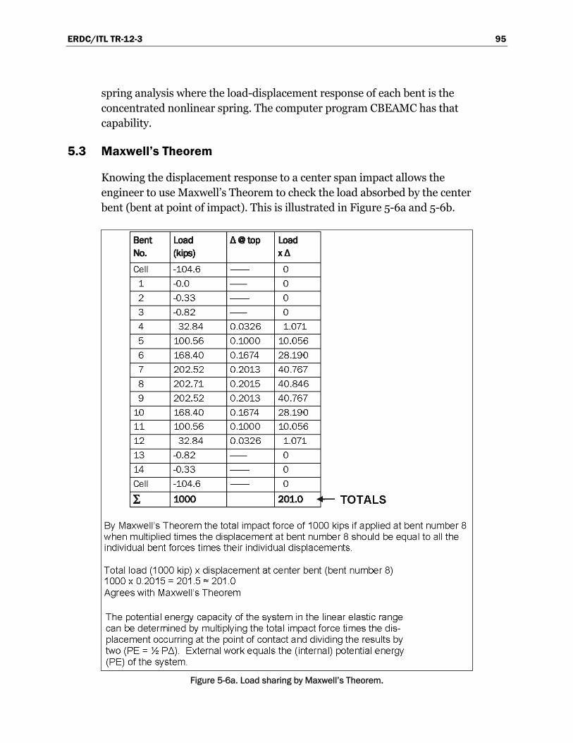
ERDC/ITL TR-12-3 95
spring analysis where the load-displacement response of each bent is the concentrated nonlinear spring. The computer program CBEAMC has that capability.
5.3 Maxwell’s Theorem
Knowing the displacement response to a center span impact allows the engineer to use Maxwell’s Theorem to check the load absorbed by the center bent (bent at point of impact). This is illustrated in Figure 5-6a and 5-6b.
Figure 5-6a. Load sharing by Maxwell’s Theorem.
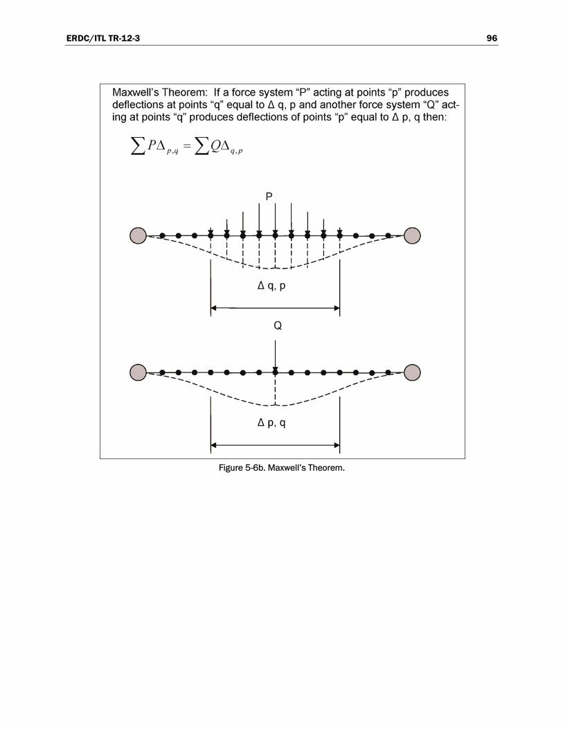
ERDC/ITL TR-12-3 96
Figure 5-6b. Maxwell’s Theorem.

ERDC/ITL TR-12-3 97
6 Conclusions and Future Research
6.1 Introduction
More than 50 percent of the Corps locks and their approach walls have continued past their economic lifetimes. As these structures wear out they need to be retrofitted, replaced, or upgraded with a lock extension. Energy absorbing flexible approach wall structural systems are being considered for these retrofits, replacements, and upgrades. The next generation flexible structures feature reduces replacement costs as well as provides additional protection for barge train traffic and barge train personnel.
Innovative flexible structures would provide cost savings by taking advantage of “in-the-wet” construction. Flexible structures would help to protect barge train traffic by “flexing” to absorb energy from impacts in order to maintain barge train integrity, and reduce the possibility of broken lashings and runaway barges.
The engineering procedures contained within this report make use of flexible pile-founded substructures for energy absorption. Two different impact approach wall flexible substructure piling systems have been considered and discussed:
Reinforced concrete impact beams spanning between (vertical) drilled-in-piles (DIP) bents;
Reinforced concrete impact walls spanning bents including batter-piles (BP).
The load versus deformation characteristics of the two impact wall systems will depend on the loading configuration and its magnitude, as well as numerous aspects of the pile supports in the substructure (e.g., geometry, capacities, limits, fixities, and the stiffness of the pile system) and the engineering characteristics of the soil (or rock) foundation (e.g., strength and stiffness).
Guide walls, guard walls, and other impact wall systems adjacent to naviga-tion locks must be capable of absorbing and dissipating energy in a manner consistent with performance objectives established for usual, unusual, and extreme barge impact events. Serviceability performance is required for

ERDC/ITL TR-12-3 98
usual barge impact events, damage control performance is required for unusual barge impact events, and collapse prevention performance that is required for extreme barge impact events. Energy dissipation for extreme events is often accompanied by nonlinear behavior, especially in approach wall systems that are not protected by adequate energy absorbing fendering systems.
6.2 Conclusions
A pushover capacity analysis combined with a balance of energy approach has been developed to generate a non-linear load versus displacement relationship for specified pile-founded flexible approach wall system.
Various failure mechanisms have been identified that need to be evaluated during a pushover capacity analysis for a pile group. These failure mechan-isms include yielding of individual piles (e.g., below the mud line), flexural failure of connections of pile to the pile cap, failure of the soil by pull-out, and soil bearing failure due to pile plunging. Non-linear load versus deflec-tion relationships result when these failure mechanisms develop. When a sufficient number of mechanisms occur among the piles, structural instability will result and the structure will no longer be able to support additional loading. In this way, the engineer will be able to determine if a pile-founded structural system will be able to withstand usual, unusual, and extreme load conditions.
CPGA has been shown to be a viable and robust software tool for performing pushover capacity analyses of pile-founded flexible approach wall systems. Examples of pile-founded approach wall systems with bents containing vertical piles exclusively and bents combining batter piles with vertical piles have been analyzed successfully to determine load versus deflection non-linear relationships:
For an example pile bent consisting exclusively of vertical piles in dry and wet conditions, pushover analyses were performed with three analytical techniques: the Yang (1966) approach, the nonlinear p-y curve approach, and the Saul (1968) approach (as implemented in the computer software CPGA). The load versus deflection curves for the CPGA analyses compared favorably with the curves developed with the other two approaches.
For an example pile bent consisting of vertical and batter piles in dry conditions, pushover analyses were performed with two computer

ERDC/ITL TR-12-3 99
software packages: GROUP7 and CPGA. The load versus deflection curve for the CPGA analysis compared favorably with the curve developed with GROUP7.
Preliminary research using a 3-D analytical procedure has shown that, when the impact deck system is structurally detailed to accommodate load sharing among multiple pile bents, loading on any individual pile bent is reduced from the case when an individual pile bent must resist the entire impact loading or the case of a simply supported impact beam supported on each end by a pile bent.
6.3 Future research
6.3.1 Background
The current guidance for determining the soil-to-pile interaction para-meters is given by the engineering manual EM 1110-2-2906, published in 1991. There has been no Corps guidance documents published on this topic since that time. EM 1110-2-2906 (1991) is geared toward pile founded locks, dams and spillway structures. These types of hydraulic structures have traditionally been constructed “in-the-dry”, involve far larger groups of pilings than flexible approach walls and rest directly on the soil foundation. These are a different type of hydraulic structure than the next generation flexible approach wall. However, some information contained within this engineering manual is relevant to the design of the flexible approach walls. Relevant EM 1110-2-2906 (1991) guidance and observations on soil-to-pile interaction parameters is as follows:
a. Soil and Pile Properties. The soil-pile stiffness is a function of the pile structural properties, soil properties, degree of pile restraint against rota-tion, and pile-head movement. The pile properties needed to determine the spring stiffnesses are the modulus of elasticity, moment of inertia, cross-sectional area, width, and length. The soil properties needed to determine the spring stiffnesses are the undrained shear strength or angle of internal friction, and the unit weight. An estimate of pile-head movement is needed to determine the linear spring stiffnesses. This is accomplished by using a secant modulus corresponding to an estimated pile-head movement. If the calculated pile head movements agree reasonably with the estimated values, then the solution is acceptable; if not, then a new estimate of pile head movements must be used. Paragraph 4-2e in EM 1110-2-2906 (1991) discusses displacement limitations at the pile cap for proper operations at

ERDC/ITL TR-12-3 100
locks and dams. These limitations should be maintained in the calculated pile head movements.1
b. Axial Stiffness. The axial pile stiffness is expressed as:
AE
b CL
=33 33 (6.1)
where:
b33 = axial pile stiffness; C33 = constant which accounts for the interaction between the soil
and the pile; A = cross-sectional area of the pile; E = modulus of elasticity of the pile; L = length of the pile.
The term AE/L is the elastic stiffness of the pile acting as a short column with no soil present. The coefficient (C33) accounts for the stiffness of the soil-pile system. An overview of various soil-to-pile relationships for vertical piles between axial load capacity, movements of the pile head and tip, and load transfer along the shaft of friction piles is presented in Chapter 2 of Mosher and Dawkins (2000). These relationships are used in simplified one-dimensional numerical analyses of axially loaded piles to predict the distribution of pile movement (relative to the soil) and the shear transfer along the length of the pile. Some of these formulations are implemented in the 1984 CASE software CAXPILE (Dawkins 1984).
a. For design purposes, C33 for a compression pile ranges between 1.0 and 2.0 although values as low as 0.1 and as high as 3.0 have been noted in the literature. There appears to be a relationship between C33 and pile length. Longer piles tend to have higher values of C33 than shorter piles. C33 for tension piles in sand can be taken as one half of the value used for compression piles. For tension piles in clay, use 75 to 80 percent of the value of C33 for compression piles.
1 It is cautioned that this EM 1110-2-2906 displacement guidance needs to be adapted for use with next generation, flexible approach walls. Specifically, loadings of the impact beam or deck can occur tens of feet above the pile-to-soil foundation interface. The additional deflections that occur in these piles where the pile extends above the ground surface will need to be accounted for in the displacement criteria for flexible approach walls. This will be part of this next research effort.

ERDC/ITL TR-12-3 101
b. Long-term loading, cyclic loading, pile group effects, and pile batter can affect C33. In sand, long-term loading has little effect on the value of C33; however consolidation in clay due to long-term loading can reduce C33. At present, the effect of cyclic loading on C33 is neglected. For design purposes, if piles are driven to refusal in sand or to a hard layer, there is no change in the value of C33 for pile groups; however, C33 may be reduced for groups of friction piles.
c. The value of C33 for single piles can be calculated using the following equation:
Δ
Cδ
=33 (6.2)
where:
∆
= axial movement of the pile head due to axial load P P = allowable axial design load for the pile
For axial stiffness, the load-deflection curve is essentially linear to one-half of the ultimate pile capacity (the design load), so nonlinearity of the axial pile stiffness can be neglected. Methods for calculating C33 from the above equations include empirical methods (Vesic 1977), Winkler foundation analysis (Scott 1981), t-z curve analyses (Mosher 1984; Coyle and Reese 1966; Coyle and Sulaiman 1967; Kraftet al. 1981; and Vijayrergiya 1977), finite element methods, and elastic method (Poulos and Davis, 1980).1 Values of C33 can be determined most accurately from pile load tests, where C33 can be determined to approximate the linear portion of the pile load-deflection curve.2
1 In the post- EM 1110-2-2906 time frame (i.e., since 1991), the authors of this research report were
unable to locate any studies of this nature. This type of research is still needed and will therefore be part of this next research effort.
2 Pile load tests are expensive. They have been justified on previous Corps projects when a very large amount of production piles are used, such as in the foundations of locks, dams, and/or spillways. The authors of this report question the practicality of in-the-wet pile load tests to determine the value for the C33 term due to increased costs of testing in-the-wet and considering the fewer number of piles involved for flexible approach walls.

ERDC/ITL TR-12-3 102
6.3.2 Extending the research
“In the wet” driving of piles requires driving piles from a barge or barges. A pile driving operation with the crew working on the water is more expensive that “in-the-dry” construction. Moving the pile driving crane barge across the project site during piling installation, as well as providing for delivery of the piling and other construction materials, requires the use of supply barges and a tow boat. All of these items add additional expense. Consideration of the expense of the placement of a pile foundation using “in the wet” construction is the motivation for the research discussed in this subsection. The research objective is to minimize the length of piles required for pile bents of flexible approach walls to minimize costs. This goal will be achieved by determining the engineering design procedures for vertical and for batter pile groups that provide for the minimum length of pile embedment while satisfying Corps design criteria1.
Barge train impact events with Flexible Approach Wall impact beams and impact decks occur far above the top-of-soil, foundation level. The 1991 guidance document for the design of pile foundations (EM 1110-2-1906) is geared towards a different type of hydraulic structure; pile founded locks, dams, and spillway structures. These types of hydraulic structures have traditionally been constructed “in-the-dry”, involve far larger groups of pilings than flexible approach walls, and rest directly on the soil foundation. Groups of vertical piles for flexible approach walls involve a far smaller pile group, have been typically oriented in a single row along a line perpen-dicular to the face of the impact wall and extend above the ground surface. This contrasts with the piling footprint that extends in both directions (when viewing in plan) under the base of soil-founded lock, dam and spillway monoliths. This “forest” of piling in two-dimensions allows for “redundancy” and load sharing among neighboring piles so that the design procedure being used to account for group response effects does not have to be precise. The eccentricity of horizontal loading of flexible approach walls relative to the region of soil-pile interaction response, in conjunction with a far smaller group of “in-line” piles, means that proper assessment of soil loading, lateral pile deformations, and pile-to-pile interactions are very important to the assessment of pile depth and size requirements. There is far less “redundancy” in this smaller, more “one-dimensional” pile group alignment. These issues are not addressed in EM 1110-2-1906 (1991) as they pertain to the design of next-generation flexible approach walls. 1 Flexible Approach Walls are designed for Usual, Unusual, and Extreme barge train impact loadings.

ERDC/ITL TR-12-3 103
Accurately accounting for pile shadowing effects of an “in-line” pile group is very important to the design of flexible approach walls. This knowledge and design procedure gap will be closed by additional research for devising the most accurate engineering procedure(s) to determine minimum pile embedment lengths. Pile bents with single or parallel rows of “in-line” groups of vertical piles will be investigated. In addition, batter piles in pile bents resisting the barge train impacts with flexible approach walls will also be investigated. Longitudinal and transverse pile-to-soil-to-pile interactions become far more important when dealing with these smaller “in-line” pile groups for the next generation flexible approach walls.
The items for subsequent research in this flexible approach walls research program are:
a. Conduct complete Soil-Structure Interaction (SSI) 3-D finite element modeling (FEM) of pile systems to provide quantitative information for modifying, as necessary, the discussion of pile proximity effects (sometimes called “pile shadowing”) in Chapter 3, section 3.9 (especially Figure 3-22). The quantitative information will include properties based on varying soil types and with differing load conditions. Davisson (1970) discussed “pile shadowing” effects, or the effects of pile-to-soil-to-pile interactions that occur when piles are in close proximity. In this discussion, Davisson provided an estimation of pile shadowing effects that varied based on the distance between pile centers normalized by the pile diameter. In-line1 pile shadowing effects varied from 3-pile diameters to 8-pile diameters with pile shadowing effects diminished at 8-pile diameters, as shown in Table 3.4 (from EM 1110-2-2906 1991). The relationship for pile shadowing effects that is given in Table 3-4 and Davisson guidance is without reference to field measurements or analytical results. Pile shadowing is an important issue for SSI analysis of pile founded approach walls using CPGA, especially for flexible approach walls. Both the Davisson guidance as well as Table 3-4 criteria (from EM 1110-2-2906 1991) is presented without supporting site-specific or analytical data and without guidance on the (statistical) variance about the relationship. With a suite of generalized sites (for homogenous and layered soils), Figures 3-22
1 In-line pile effects are defined to be the effects that occur between piles in a bent that are along the
line of action of the applied load.

ERDC/ITL TR-12-3 104
and 3-231 and Table 3-4 in-line and perpendicular relationships, will be refined and made more accurate using 3-D FEM analysis results (Figure 6-1). This effort will include an assessment that will result in a characterization of the dispersion contained within the resulting relationship.
Figure 6-1. 3-D finite element model of a loaded pile bent founded in layered soils.
b. CPGA is an important analytical tool for evaluating the response of groups of piles in soil to applied loads. The input values assigned to the soil-to-pile interaction parameters have a large impact on computed results. The user provided value for C33 is an important parameter for axial SSI response, especially for batter piles systems where the elastic center of the pile group is non-coincident with the resultant force line of action. Complete 3-D SSI finite element analyses of pile groups are essential for developing guidance for the accurate assignment of the site-dependent C33 stiffness term in the CPGA simplified model (shown in Figure 6-2). The suite of 3D FEA analyses will be performed with input of varying soil types and differing loading conditions, as well as pile geometry to include proximity effects. A statistical assessment of the range in C33 term values will be developed (i.e., mean, standard deviation, and distribution) for the soil foundation using 3-D finite element Complete SSI pile group response analysis results. These results will then be adapted and included in a new Reliability
1 Figure 3-23 shows the curve fit for field measurements (with differing soil types and load conditions)
for loads that were applied perpendicular to a row of piles in a bent.

ERDC/ITL TR-12-3 105
version of the CPGA software. The Reliability method of analysis is a statistical method of analysis that formally accounts for uncertainties in the parameters that impact the results computed by CPGA and provide insight into the probability of unsatisfactory performance for the structural system being analyzed. The goal of the engineering evaluation is to specify the procedure requiring the minimum depth of pile embedment that satisfies Corps design criteria.
Figure 6-2. Actual approach wall design and corresponding simplified model.
c. Four plausible engineering methodologies, including Davisson’s simplified relationships for minimum “long pile” behavior, were identified in this report. These methodologies may be used to determine the depth of embedment for vertical piles subjected to lateral loading. Considering the expense for placement of a pile foundation “in-the-wet”, additional research into guidance for minimum depth of embedment criteria for vertical piles is warranted. This additional research will include the determination of the optimum procedure of the three procedures discussed in Section 3.3 for interpreting the results of nonlinear SSI analyses (e.g., using COM624G) for determining the minimum depth of embedment for vertical piles.
d. CPGA is limited to modeling the response of groups of piles connected to a “rigid” pile cap. Impact decks are more likely to be “flexible” than “rigid”. Analyses will be made to determine how SSI responses will be affected by the addition of a flexible pile cap in the model, including proximity effects. An evaluation of the importance of “flexible” pile caps on the SSI response of pile groups will be performed and the need for including a flexible pile cap in the model will be assessed.
e. The simplified model that has been discussed (CPGA) is limited to static pile group analysis (with constant applied loads and/or moment). A

ERDC/ITL TR-12-3 106
formulation will be developed for the dynamic structural time-history analysis of an impact beam-pile founded system and corresponding software (e.g., Impact_Deck) for use by District Engineers. Recall that Impact_Force software (Ebeling et al. 2010) allows for the development of a barge train specific impact force pulse time-history that can be used as input to Impact_Deck. This will allow District Engineers to design and analyze two flexible approach wall system features in a single dynamic analysis (i.e., both the flexible pile groups and the flexible approach wall structural system) for a realistic barge impact. This formulation accounts for flexible response from the pile group substructure and the flexible impact beam superstructure that allows load-sharing between pile bents. The Impact_Deck software will allow for different pile group configurations (i.e., vertical and batter bents with piles that are in-line or 2-D in plan, as seen in the plan view of Figure 6-3) and for various deck and/or beam configurations (i.e., different structural boundary conditions at joints). Load-sharing between pile bents will allow for a more optimal determination of pile bent layout (e.g., number of piles and their geometry), spacing between pile bents, and individual drilled in place pile diameters (or pile sizes for driven piles) and embedment depths. All of these features contribute to lower construction costs.
The results of these research efforts will be published in subsequent ERDC Technical Reports and the PC-based software will be distributed through the ERDC CASE Library (http://case.wes.army.mil/).

ERDC/ITL TR-12-3 107
Figure 6-3. Example problem for Impact_Deck with dynamic impact force time-history.

ERDC/ITL TR-12-3 108
References
ACI 318. 2002. American Concrete Institute. Building Code Requirements for Structural Concrete (ACI 318) Box 19150, Redford Station, Detroit, MI 48219.
ACI Committee 336. 1972. American Concrete Institute Committee 336 Report, Suggested Design and Construction Procedures for Pier Foundations, ACI Box 19150, Redford Station, Detroit, MI 48219
Anderson, A. R., and S. E. Moustafa. 1970. Ultimate Strength of Prestressed Piles and Columns, ACI Journal, 1970.
Arroyo-Caraballo, J. R., and R. M. Ebeling. 2006. Glancing-Blow Impact Forces by a Barge Train on a Lock Approach Wall. ASCE Journal of Infrastructure Systems, 12(2):135-143.
Arroyo-Caraballo, J. R., R. M. Ebeling, and B. C. Barker. 2003. ERDC/ITL TR-03-3. Analysis of Impact Loads from Full-Scale Low-Velocity, Controlled Barge Impact Experiments.
Broms, B. B. 1965. Design of laterally loaded piles. ASCE Journal of the Soil Mechanics and Foundations Division, Vol. 91, No. SM 3, 1965 (May), pp. 79-99.
Budek, A. M., M. J. N. Priestley, and G. Benzoni. 2000. Inelastic Seismic Response of Bridge Drilled-Shaft RC Pile/Columns, ASCE Journal of Structural Engineering.
Castello, R. R. 1980. Bearing capacity of driven piles in sand. Ph.D. Thesis, Texas A&M University, College Station, Texas.
Chopra, A. K. 1995. Dynamics of Structures, Theory and Applications to Earthquake Engineering. Prentice-Hall Inc. Upper Saddle River, NJ 07458, 1995
Coyle, H. M., and L. C. Reese. 1966 (Mar). Load-Transfer for Axially Loaded Piles in Clay. Journal, Soil Mechanics and Foundations Division, American Society of Civil Engineers, Vol 92, No. SM2, pp 1-26.
Coyle, H. M., and I. H. Sulaiman. 1967 (Nov). Skin Friction for Steel Piles in Sand. Journal, Soil Mechanics and Foundations Division, American Society of Civil Engineers, Vol 93, No. SM-6, pp 261-278.
Cox, W. R., D. A. Dixon, and M. W. O’Neil. 1984. Lateral load tests of 25.4 mm diameter piles in very soft clay in side-by-side and in-line groups, Laterally Loaded Deep Foundations: Analysis and Performance. ASTM. STP835.
Davisson, M. T. 1963 (July). Estimating Buckling Loads for Piles. Proc. Second Pan American Conference on Soil Mechanics and Foundation Engineering, Vol. 1, pp. 351-71.
Davisson, M. T. 1970. Lateral Load Capacity of Piles. Highway Research Record, Number 133, Pile Foundations, Highway Research Board, Washington DC

ERDC/ITL TR-12-3 109
Dawkins, W. P. 1984. Users Guide: Computer Program for Soil-Structure Interaction Analysis of Axially Loaded Piles (CAXPILE). Technical Report K-84-4. US Army Engineer Waterways Experiment Station, Vicksburg, MS.
Dawkins, W. P. 1994. Users Guide: Computer Program for Analysis of Beam-Column Structures with Nonlinear Supports (CBEAMC). Instruction Report ITL-94-6. US Army Engineer Waterways Experiment Station, Vicksburg, MS.
Derecho, A. T., D. M. Schultz, and M. Fintel. 1978. Analysis and Design of Small Reinforced Concrete Buildings for Earthquake Forces. Portland Cement Association.
Ebeling, R. M., A. N. Mohamed, J. R. Arroyo, B. C. White, R. W. Strom, and B. C. Barker. 2011. Dynamic Structural Flexible-Beam Response to a Moving Barge Train Impact Force Time-History Using Impact_Beam. EDRC/ITL TR-11-1. Department of the Army, Army Corps of Engineers, Engineer Research and Development Center, Vicksburg, MS.
Ebeling, R. M., B. C. White, A. N. Mohamed, and B. C. Barker. 2010. Force Time History During the Impact of a Barge Train with a Lock Approach Wall Using Impact_Force. EDRC/ITL TR-10-3. Department of the Army, Army Corps of Engineers, Engineer Research and Development Center.
Engineering Manual. EM. 1110-2-2104. 1992. Strength Design for Reinforced-Concrete Hydraulic Structures, US Army Corps of Engineers, Washington, DC 20314-1000.
Engineering Manual. EM 11110-2-2906. 1991. Design of Pile Foundations, US Army Corps of Engineers, Washington, DC 20314-1000.
Engineering Manual. EM 1110-2-2100. 1995. Stability Analysis of Concrete Hydraulic Structures, US Army Corps of Engineers, Washington, DC 20314-1000.
ETL 1110-2-563. 2004. Barge Impact Analysis for Rigid Walls. US Army Corps of Engineers, Washington, DC 20314-1000
ETL 1110-2-338. 1993. Barge Impact Analysis. US Army Corps of Engineers, Washington, DC 20314-1000
Ehsani, M. R., and M. E. Marine. 1994. User’s Guide for Moment-Curvature Relationship (M-PHI). US Army Corps of Engineers Contract Report SL-94. MRE and Associates, Tucson, AZ 85715.
FEMA 356. 2000. Prestandard and Commentary for the Seismic Rehabilitation of Buildings, Federal Emergency Management Agency, Washington, DC.
FEMA 356. 2000. Prestandard and Commentary for the Seismic Rehabilitation of Buildings. Federal Emergency Management Agency, Washington, DC.
FHWA-IP-87-6. May 1987. U.S. Department of Transportation, Federal Highway Administration. Seismic Design and Retrofit Manual for Highway Bridges
Feygin, V. B., and R. J. Mancini. 2012. Seismic Design of Pile-to-Pile Cap Connections in Flexible Pier Structures. Structure Magazine, pp. 21-24, 2012 (March)

ERDC/ITL TR-12-3 110
Gaythwaite, J. W. 2004. Design of Marine Facilities for Birthing, Mooring, and Repair of Vessels, 2nd edition. published by American Society of Civil Engineers, Reston, VA, 2004.
Goyal, A., and A. K. Chopra. 1989. Earthquake Analysis and Response of Intake Towers. Report No. UBC/EERC-89-04. Earthquake Engineering Research Center, University of California, Berkeley, California.
Harn, R. E. 2004. Displacement Design of Marine Structures on Batter Piles, 13th World Conference on Earthquake Engineering. Vancouver, B.C. Canada, Paper 543.
Hartman, J. P., J. J. Jaeger, J. J. Jobst, and D. K. Martin. 1989. User’s Guide: Pile Group Analysis (CPGA) Computer Program X0080. Technical Report ITL-89-3. US Army Engineer Waterways Experiment Station, Vicksburg, MS.
Headquarters, U.S. Army Corps of Engineers (HQUSACE). 2005. Stability Analysis of Concrete Structures. EM 1110-2-2100. Washington, DC.
Headquarters, Department of the Army. 2004. Barge impact analysis for rigid walls. Engineer Technical Letter 1110-2-563. Washington, DC
Kraft, L. M., J. A. Focht, and S. F. Amerasinghe. 1981 (Nov). Friction Capacity of Piles Driven Into Clay. Journal, Geotechnical Engineering Division, American Society of Civil Engineers, Vol 107, No. GT11, pp 1521-1541.
Lien, B. 2011. Where is the Fixity below Top of an Embedded Laterally Loaded Pile or Drilled Shaft?, The 6th Geotechnical, Geophysical and Geoenvironmental Technology Transfer Conference and Expo. Raleigh, North Carolina.
Lieng, J. T. 1988. Behavior of Laterally Loaded Piles in Sand – Large Scale Model Tests. Ph.D. Thesis. Department of Civil Engineering, Norwegian Institute of Technology, 206 pages.
MathCAD 8, 1998 (August). Mathsoft, Inc., Cambridge, MA.
Mosher, R. L. 1984 (Jan). Load-Transfer Criteria for Numerical Analysis of Axially Loaded Piles in Sand, Part 1: Load-Transfer Criteria. Technical Report K-84-1. US Army Engineer Waterways Experiment Station, Vicksburg, MS.
Mosher, R. L., and W. P. Dawkins. 2000. Theoretical Manual for Pile Foundations. Technical Report ERDC/ITL TR-00-5, Department of the Army, Army Corps of Engineers, Engineer Research and Development Center, Vicksburg, MS.
Naaman, A. E., H. H. Harajli, and J. K. Wright. 1986. Analysis of Ductility in Partially Prestressed Concrete Flexural Members. PCI Journal.
Paz, M. 1991. Structural Dynamics, Theory and Computation. Third Edition, Van Nostrand Reinhold, New York.
Poulos, H. G., and E. H. Davis. 1980. Pile Foundation Analysis and Design. Wiley, New York.
Prakash, S. 1962. Behavior of Pile Groups Subjected to Lateral Loads. Unpublished Dissertation, University of Illinois.

ERDC/ITL TR-12-3 111
Price, W. A., M. D. Davister, and M. E. George. 1984. User’s Guide for Strength Analysis of Non-Hydraulic Structural Elements, Report 1, Concrete General Strength Investigation (CGSI). Corps Program X0061, Instruction Report K-84-10, US Army Engineer Waterways Experiment Station, Vicksburg, MS,.
Priestley, M. J. N., F. Seible, and G. M. Calvi. 1996. Seismic Design and Retrofit of Bridges, John Wiley & Sons, Inc.
Rangan, B. V., and M. Joyce. 1992. Strength of Eccentrically Loaded Slender Steel Tubular Columns Filled with High-Strength Concrete. ACI Structural Journal.
Reese, L. C., L. A. Cooley, M. W. and N. Radhakrishnan. 1984. Laterally Loaded Piles and COM624G Computer Program I0012), Technical report K-84-2, U.S. Army Waterways Experiment Station, Vicksburg, MS, April 1984
Reese, L. C., M. W. O’Neill, and N. Radhakrishnan. 1970. Rational Design Concept for Breasting Dolphins. ASCE Journal of the Waterways and Harbors Division.
Reese, L. C., S. T. Wang, and J. L. Fouse. 1992. Use of Drilled Shafts in Stabilizing a slope. ASCE Stability and Performance of Slopes and Embankments-II, Volume 2. Proceedings of a Speciality Conference sponsored by the Geotechnical Engineering Division of the American Socielty of Civil Engineers, ASCE, Geotechnical Special Publication No. 31, pp. 1318-1332.
Reese, L. C., S. T. Wang, J. A. Arrellaga, J. Hendrix, and L. Vasquez. 2006 (February). Computer Program Group Version 7, A Program for the Analysis of a Group of Piles Subjected to Axial and Lateral Loading. Ensoft, Inc., Austin, Tx
Saul, W. E. 1968. Static and Dynamic Analysis of Pile Foundations. Journal of the Structural Division. ASCE, Volume 94, Number ST5, Proceeding Paper 5936, May 1968
Scott, F. S. 1981. Foundation Analysis, Prentice-Hall, Englewood Cliffs, NJ.
Semple, R. M., and W. J. Rigden. 1984(Oct). Shaft Capacity of Driven Pile in Clay. Analysis and Design of Pile Foundations, American Society of Civil Engineers, J.R. Meyer, Ed., pp 59-79
Sheppard, D. A. 1983. Seismic Design of Prestressed Concrete Piling, PCI Journal
Skogman, B. C., M. K. Tadros, and R. Grasmick. 1988. Ductility of Reinforced Concrete Flexural Members. PCI Journal
Strom, R. W., K. Abraham, and H. W. Jones. 1996. User’s Guide: Concrete Pile Analysis (CPGA) Computer Program X0088. Technical Report ITL-90-2. US Army Engineer Waterways Experiment Station, Vicksburg, MS.
Strom, R. W., and R. M. Ebeling. 2005 Seismic Structural Considerations for the Stem and base of Retaining Walls Subjected to Earthquake Ground Motions. EDRC/ITL-05-3. Department of the Army, Army Corps of Engineers, Engineer Research and Development Center, Vicksburg, MS
ERDC/ITL TR-12-3 112
Strom, R. W., and R. M. Ebeling. 2001 (Dec). State of Practice in the Design of Tall, Stiff and Flexible Tieback Retaining Walls. ERDC/ITL TR-01-1. Department of the Army, Army Corps of Engineers, Engineer Research and Development Center, Vicksburg, MS.
Terzaghi, K. 1955. Evaluation of coefficient of subgrade reaction. Geotechnique, Vol. 5, pp. 297-326.
Tschebotarioff, G. P. 1973. Foundations, Retaining and Earth Structures, The Art of Design and Construction and Its Scientific Basis in Soil Mechanics. Second Edition. McGraw-Hill Book Company, New York, NY.
Terzaghi, Z., and R. B. Peck. 1967. Soil Mechanics in Engineering Practice. Second Edition. Wiley, New York.
Technical Manual. TM 5-809-10-1. 1986. Seismic Design Guidelines for Essential Buildings, Departments of the Army, Navy and Air Force.
The CASE Task Group on Pile Foundations. Technical Report. K-83-1. 1983. Basic Pile Group Behavior, US Army Engineer Waterways Experiment Station, PO Box 631, Vicksburg, MS 391809
Tsinker, G. 2004. Port Engineering, Planning, Construction, Maintenance and Security. John Wiley and Sons, New York, NY, 2004.
Vesic, A. S. 1977. Design of Pile Foundations. National Cooperative Highway Research Program, Synthesis of Highway Practice No. 42, Transportation Research Board, Washington, DC.
Vijayrergiya, V. N. 1977 (Mar). Load - Movement Characteristics of Piles. Ports ’77, Proceedings, 4th Annual Symposium of the Waterways, Port, Coastal and Ocean Division of American Society of Civil Engineers, Vol 2, pp 269-284.
Wang, S. T., and L. C. Reese. 1984. Study of design methods for vertical drilled shaft retaining walls. Texas Department of Highways and Public Transportation, Austin, Texas.
Yang, N. C. 1966. Buckling Strength of Pile. Highway Research Record, Number 147, Bridges and Structures. Highway Research Board. Washington DC

ERDC/ITL TR-12-3 113
Appendix A: Pushover analysis of drilled-in caisson, Fixed-head system Using Yang (1966), Saul (1968) and nonlinear p-y curve analysis
A.1 Fixed-head system to be used in the pushover analyses
A fixed-head approach wall impact system supported on 6-ft diameter drilled-in caissons is illustrated in Figures A-1 and A-2. This bent structural system, consisting of pairs of drilled in place piles placed 27 ft on center will be analyzed in three pushover analyses in this appendix. The appendix concludes with a comparison of results from three engineering calculation methods based on Yang (1966), Saul (1968) using CPGA, and nonlinear p-y analysis using COM624G.
For the pushover analyses model used in the CPGA and COM624G analyses, the total length of the pile specified was 100 ft (1200 in.), with 40 ft (480 in.) being the unembedded length and 60 ft being the embedded length. Because this embedded length is longer than the longest Le values from Table 3-3 in Chapter 3, “long pile” behavior is accurately modeled. Recall that “long pile” behavior results when further lengthening of the pile will result in the moment and shear at the lower end (i.e., tip) of the flexible pile being negligible (see Figure 2 in Davisson, 1970).
Figure A-1. Plan view - approach wall monolith.
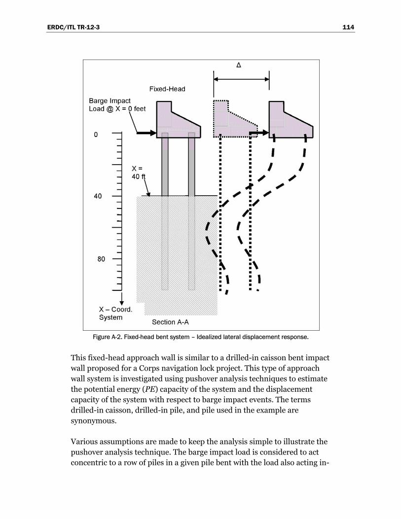
ERDC/ITL TR-12-3 114
Figure A-2. Fixed-head bent system – Idealized lateral displacement response.
This fixed-head approach wall is similar to a drilled-in caisson bent impact wall proposed for a Corps navigation lock project. This type of approach wall system is investigated using pushover analysis techniques to estimate the potential energy (PE) capacity of the system and the displacement capacity of the system with respect to barge impact events. The terms drilled-in caisson, drilled-in pile, and pile used in the example are synonymous.
Various assumptions are made to keep the analysis simple to illustrate the pushover analysis technique. The barge impact load is considered to act concentric to a row of piles in a given pile bent with the load also acting in-
ERDC/ITL TR-12-3 115
line with the axis of the cap beam as shown in Figures A-1 and A-2. The cap beam is assumed to act as a rigid member.
It has been observed in the analyses to be described that for this fixed-head (two-pile bent) system, flexural hinges are likely to first form at the pile to cap connections followed by flexural hinging in each pile below the mudline. For the fixed-head system a collapse mechanism is proposed to be reached after hinges below the mudline have reached ultimate rotation capacity. However due to the difficulty in inspecting for this action in piles below the mudline and, the cost for repair/replacement and the disruption in usage, this type of performance is objectionable except for highly unlikely extreme barge impact events. This pushover analysis calculation assumes that other mechanisms such as pile pullout, pile shear, etc. do not occur.
A sand foundation with a stiffness that varies linearly with depth is investi-gated. The coefficient of subgrade reaction (nh) is assumed to be 50 pci. This value for nh is corresponds to Terzaghi’s (1955) “recommended” value for a moist medium-dense sand and within the scatter considering nh values cited in other technical literature (e.g., Davisson, 1970).
Flexural moment capacity is a function of axial load. The axial load ratio for large drilled-in-caissons are likely to be low for approach walls, so the axial load effects with respect to increased moment capacity will be low. The influence of axial load on moment capacity can be evaluated by axial load – moment interaction analysis of moment curvature analysis. This is demonstrated later in this Appendix.
A.2. Pile properties
Concrete compressive strength: f’c = 4000 psi Concrete modulus Ec = w1.5 33 (f’ c)1/2 = 504,000 ksf =
3500 ksi Diameter of drilled-in pile (DIP) Dp = 6.0 ft = 72.0 in Area of DIP Ap = 28.274 ft2 = 4070 in2 Moment of inertia of DIP Ip = π (Dp)4 ÷ 64 = 63.617 ft4 =
1,319,160 in4 Effective moment of inertia of DIP Ie = 0.25 (Ip) = 15.90 ft4 =
330,000 in4

ERDC/ITL TR-12-3 116
A.3. Nominal moment capacity of drilled-in piles
Flexural hinge moment capacity depends on the axial load in the caisson which changes with each lateral barge impact load increment for the fixed-head two-pile bent system. The levels of axial load representing the point of first yield will be estimated assuming the impact beam weight and pile weight to mudline is equally distributed to the impact side and far side caissons. These computations are provided in Figure A-3.
Figure A-3. Section view - Approach wall monolith.

ERDC/ITL TR-12-3 117
The flexural capacity at the top and bottom of each pile is determined first using the Corps M-PHI Computer Program X2002. An axial load – moment interaction analysis is also performed to establish moment capacity using the Corps CGSI Computer Program X0061. The pile section with reinforce-ment to be evaluated by moment – curvature and load – moment interac-tion is illustrated in Figure A-4.
Figure A-4. 6-ft diameter drilled-in caisson section.
The Corps computer program M-PHI is first used to determine the moment capacities at the plastic hinge located at the pile cap and below the mudline based on the simplifying assumptions for axial load described above. These moment curvature analyses are provided below.

ERDC/ITL TR-12-3 118
Axial load – moment interaction points for the Figure A-4 pile section is generated using the Corps Program CGSI. Input and output are provided below.
M-PHI Input and Output for Axial Load at Top of Pile (960 k) DP1 6-FOOT DIA DRILLED PILE 1 60.0 29000.0 0.01 0.05 60.01 4.0 3500.0 0.003 50 4 4 1 72.0 1.0 6.0 18 4.50 1 960.0 36.0 MOMENT VS. CURVATURE (K-FT) CRACKING MOMENT AND CURVATURE MOMENT... 0.2555E+04 CURVATURE... 0.5249E-05 YIELDING MOMENT AND CURVATURE MOMENT... 0.9153E+04 CURVATURE... 0.5173E-04 ULTIMATE MOMENT AND CURVATURE MOMENT... 0.1199E+05 (143880 in-k) CURVATURE... 0.1420E-03
M-PHI Input and Output for Axial Load of Pile BML (1130 k) DP1 6-FOOT DIA DRILLED PILE 1 60.0 29000.0 0.01 0.05 60.01 4.0 3500.0 0.003 50 4 4 1 72.0 1.0 6.0 18 4.50 1 1130.0 36.0 MOMENT VS. CURVATURE (K-FT) CRACKING MOMENT AND CURVATURE MOMENT... 0.2691E+04 CURVATURE... 0.5520E-05 YIELDING MOMENT AND CURVATURE MOMENT... 0.9423E+04 CURVATURE... 0.5240E-04 ULTIMATE MOMENT AND CURVATURE MOMENT... 0.1222E+05 (146640 in-k) CURVATURE... 0.1387E-03
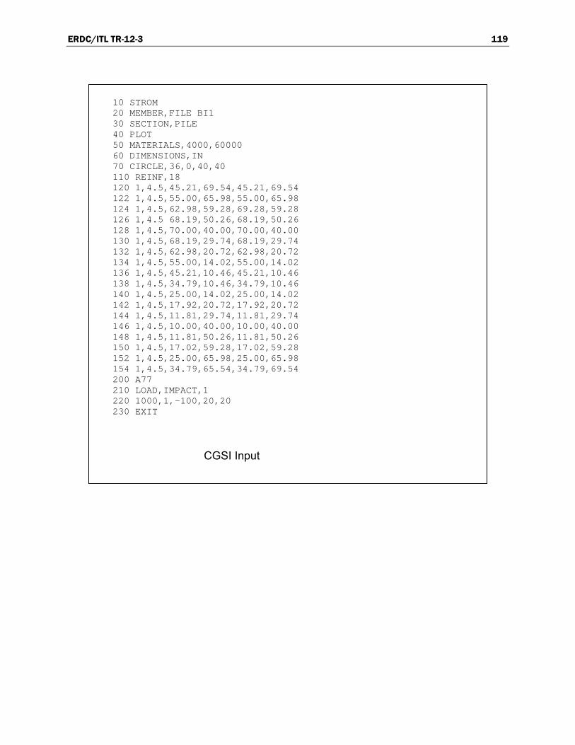
ERDC/ITL TR-12-3 119
10 STROM 20 MEMBER,FILE BI1 30 SECTION,PILE 40 PLOT 50 MATERIALS,4000,60000 60 DIMENSIONS,IN 70 CIRCLE,36,0,40,40 110 REINF,18 120 1,4.5,45.21,69.54,45.21,69.54 122 1,4.5,55.00,65.98,55.00,65.98 124 1,4.5,62.98,59.28,69.28,59.28 126 1,4.5 68.19,50.26,68.19,50.26 128 1,4.5,70.00,40.00,70.00,40.00 130 1,4.5,68.19,29.74,68.19,29.74 132 1,4.5,62.98,20.72,62.98,20.72 134 1,4.5,55.00,14.02,55.00,14.02 136 1,4.5,45.21,10.46,45.21,10.46 138 1,4.5,34.79,10.46,34.79,10.46 140 1,4.5,25.00,14.02,25.00,14.02 142 1,4.5,17.92,20.72,17.92,20.72 144 1,4.5,11.81,29.74,11.81,29.74 146 1,4.5,10.00,40.00,10.00,40.00 148 1,4.5,11.81,50.26,11.81,50.26 150 1,4.5,17.02,59.28,17.02,59.28 152 1,4.5,25.00,65.98,25.00,65.98 154 1,4.5,34.79,65.54,34.79,69.54 200 A77 210 LOAD,IMPACT,1 220 1000,1,-100,20,20 230 EXIT
CGSI Input

ERDC/ITL TR-12-3 120
Moment (Ft-k) Axial Load (k) 1010 52 1020 .00000000E+00 .14616090E+05 PO = 14616 kips 1030 .68866790E+04 .14616090E+05 1040 .75204550E+04 .14226560E+05 1050 .81205270E+04 .13837050E+05 1060 .86823940E+04 .13447520E+05 1070 .92081300E+04 .13058000E+05 1080 .97025080E+04 .12668480E+05 1090 .10167610E+05 .12278950E+05 1100 .10604900E+05 .11889430E+05 1110 .11014070E+05 .11499910E+05 1120 .11396150E+05 .11110390E+05 1130 .11752500E+05 .10720870E+05 1140 .12084640E+05 .10331350E+05 1150 .12394090E+05 .99418200E+04 1160 .12682290E+05 .95522980E+04 1170 .12950290E+05 .91627800E+04 1180 .13199400E+05 .87732540E+04 1190 .13431650E+05 .83837380E+04 1200 .13645660E+05 .79942090E+04 1210 .13839670E+05 .76046920E+04 1220 .14020900E+05 .72151670E+04 1230 .14190260E+05 .68256440E+04 1240 .14340570E+05 .64556210E+04 1250 .14345870E+05 .64361250E+04 1260 .14446430E+05 .60466060E+04 1270 .14497010E+05 .56570830E+04 1280 .14524310E+05 .52675710E+04 MB = 14524 ft-k 1290 .14468460E+05 .48780450E+04 PB = 5268 kips 1300 .14337210E+05 .44885250E+04 1310 .14189140E+05 .40990060E+04 1320 .14026960E+05 .37094790E+04 1330 .13790990E+05 .33199580E+04 1340 .13495270E+05 .29304390E+04 1350 .13181490E+05 .25409170E+04 1360 .12851670E+05 .21513940E+04 1370 .12471690E+05 .17618760E+04 1380 .12013860E+05 .13723460E+04 1390 .11511810E+05 .98283240E+03 1400 .10992570E+05 .59330760E+03 1410 .10460530E+05 .20378510E+03 MO = 10000 ft-k 1420 .98722650E+04 -.18573570E+03 1430 .92083850E+04 -.57525400E+03 1440 .85173870E+04 -.96477610E+03 1450 .78122610E+04 -.13543000E+04 1460 .70914590E+04 -.17438230E+04 1470 .63037500E+04 -.21333440E+04 1480 .54684130E+04 -.25228650E+04 1490 .46227630E+04 -.29123920E+04 1500 .37619760E+04 -.33019120E+04 1510 .28473300E+04 -.36914300E+04 1520 .19068080E+04 -.40809580E+04 1530 .89998660E+02 -.48600000E+04 PT = 4860 kips

ERDC/ITL TR-12-3 121
Both the moment curvature analyses and the axial load – moment interaction analysis give similar results. Those from the moment - curvature analyses will be used for the following pushover analyses.
A.4. Pushover analyses for fixed-head system using Yang (1966) graphical procedure of analysis – dry site
The ultimate moment capacities from the previous moment curvature analyses will be used to represent the yield points at the top and bottom of the piles. These represent average values for the impact side and far side piles. Average values are used to simplify the analysis. Recall the soil supporting the piles is a moist medium-dense sand with a coefficient of horizontal subgrade reaction (nh) equal 50 pci. The relative stiffness factor (T) is:
( ), , ,
.c e
h
E IT
n= = =55
3 500 000 330 000118 2
50 in = 9.85 ft
The coefficient of free-standing length (m) needed for the Yang (1966) analysis is equal to the free-standing length (LO) divided by the relative stiffness factor (T).
..
OLm
T= = =
404 06
9 85
The depth to fixity for a fixed-top translating can be obtained from Figure A-5 (after Figure 2 in Yang, 1966). Using this figure (provided below) it can be seen for an m-value equal to 4.06, the coefficient of effective embedment (a) is equal to 1.8 providing a depth to fixity (L) equal to 1.8 (9.851) = 17.732 ft and a total length (LT) from pile cap to point of fixity equal to 40.00 + 17.732 = 57.732 ft. Knowing that the moment capacity at the cap (MCC) is 143,880 in-k and assuming a point of inflection occurs midway between the cap and point of fixity, the horizontal load applied to the top of the pile that causes flexural yielding to occur is:
( , )
.. ( )
CChf
T
MP
L= = =
2 2 143 880415 367
57 732 12 kips

ERDC/ITL TR-12-3 122
Figure A-5. Effective embedment of pile at buckling (after Figure 2 Yang,
1966).
The moment below the mudline occurring at the time the moment at the pile to pile cap connection reaches ultimate can be determined using Figure A-6 (after Figure 7 in Yang, 1966).
From Figure A-6, it can be seen that for an m-value of 4.06, the coefficient of horizontal load capacity for a fixed top (Hf) is equal to 0.51. The moment below the mudline (Mmf) occurring at the time the moment at the pile to pile cap connection reaches ultimate is equal to:
( ) ( )( ). .
,.
hfmf
f
P TM
H= = =
415 367 9 851 1296 280
0 51in-k
The reserve moment capacity of the piles below the mudline is equal to their ultimate capacity (146,640 in-k) determined by moment curvature analysis less the moment demand (96,280 in-k), or 50,360 in-k.
Coefficient of free standing length (m)
Coef
ficie
nt o
f eff
ectiv
e em
bedm
ent (
a)

ERDC/ITL TR-12-3 123
Figure A-6. Coefficient of horizontal load capacity (after Figure 7 Yang,
1966).
Assuming pinned conditions at the top of pile since flexural moment capacity has already been reached at that location and determining by Figure A-6 that for a pinned top condition that the coefficient of horizontal load capacity (Hp) is equal to 0.21, the horizontal load at the top of the pile (Php) needed to use up the reserve moment capacity is:
( ) ( , ) .
.. ( )
r php
M HP
T= = =
50 360 0 2189 464
9 851 12 kips
The top of pile displacements associated with each increment of loading (Phf and Php) can be determined using Figure A-7 (after Figure 8 in Yang, 1966). With an m-value equal to 4.06, the coefficient of horizontal displacement (D) is equal to 15.0 for a fixed top condition and 75.0 for a pinned top condi-tion providing the following top of pile displacements for each increment of horizontal loading:
Coefficient of free standing length (m)
Coef
ficie
nt o
f hor
izon
tal l
oad
(H)
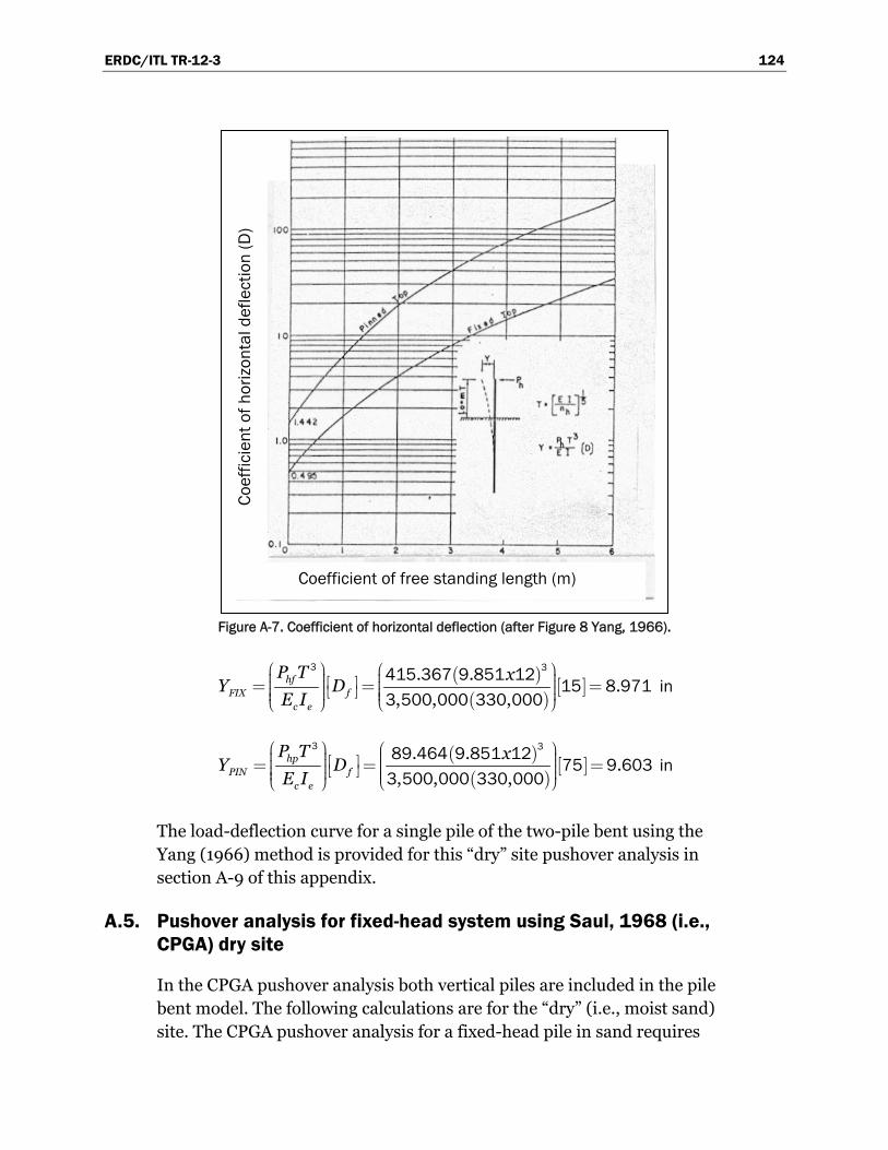
ERDC/ITL TR-12-3 124
Figure A-7. Coefficient of horizontal deflection (after Figure 8 Yang, 1966).
( )
( )[ ]
. ..
, , ,hf
FIX fc e
P T xY D
E I
æ ö æ ö÷ ÷ç çé ù÷ ÷= = =ç ç÷ ÷ë ûç ç÷ ÷çç è øè ø
3 3415 367 9 851 1215 8 971
3 500 000 330 000 in
( )
( )[ ]
. ..
, , ,hp
PIN fc e
P T xY D
E I
æ ö æ ö÷ ÷ç çé ù÷ ÷= = =ç ç÷ ÷ë ûç ç÷ ÷çç è øè ø
3 389 464 9 851 1275 9 603
3 500 000 330 000 in
The load-deflection curve for a single pile of the two-pile bent using the Yang (1966) method is provided for this “dry” site pushover analysis in section A-9 of this appendix.
A.5. Pushover analysis for fixed-head system using Saul, 1968 (i.e., CPGA) dry site
In the CPGA pushover analysis both vertical piles are included in the pile bent model. The following calculations are for the “dry” (i.e., moist sand) site. The CPGA pushover analysis for a fixed-head pile in sand requires
Coefficient of free standing length (m)
Coef
ficie
nt o
f hor
izon
tal d
efle
ctio
n (D
)

ERDC/ITL TR-12-3 125
that CPGA input items FUNSMOM and PMAXMOM be computed using Figures A-5 and A-6 above.
O
f
L aT TFUNSMOM
H
+= + = 578
2 in.
p
TPMAXMOM
H= =563 in.
For the first pushover increment a lateral load is applied at the pile cap. This load is varied until the moment in the pile at the pile to pile cap connection is at its ultimate moment capacity. The lateral load achieving this objective is something that can be obtained in short order using trial and error techniques.
The CPGA input and output for this is presented below.
In the second increment of horizontal loading, the moments at the pile to pile cap connection have reached their ultimate capacities and hinges will be introduced at that location (i.e., piles pinned at top). This can be accomplished in CPGA. The moment demand below the mudline for the first increment of loading as given by FUNSMOM is 97,975.5 in-kip.
CPGA INPUT FOR FIXED-HEAD BENT – Load increment 1 10 CANTILEVER BATTER PILE BENT FILE:DIP1 15 PROP 3500. 330000. 330000. 4070. 1.0 0.0 1 20 PROP 3500. 330000. 330000. 4070. 1.0 0.0 2 30 SOIL NH .050 L 100. 40. 1 TO 2 40 FIX 1 TO 2 50 ALLOW R 14600. 4860. 14600. 4860. 5270. 14500. 1 TO 2 70 UNSP C 0.6 0.6 14600. 14600. N 1 TO 2 80 FUNSMOM 578. 578. 1 TO 2 90 BATTER 0. 1 TO 2 100 ANGLE 0. 1 2 110 PILE 1 0. 0. 0. 120 PILE 2 20. 0. 0. 140 LOAD 1 836. 0. 960. 0. 0. 0. 190 TOUT 1 2 3 4 5 6 7 200 FOUT 1 2 3 4 5 6 7 210 PFO 1 TO 2

ERDC/ITL TR-12-3 126
In the second increment of loading the moment at the pile to pile cap connection is released and the horizontal load at the top of the piles increased (trial and error) until the reserve moment capacity equal to the moment capacity from the moment curvature analysis (146,640 in-kip) less the moment demand (97,975.5 in-kip), or 48,664 in-kip is reached. The input and output for this is provided below.
CPGA INPUT FOR FIXED-HEAD BENT– Load increment 2 10 CANTILEVER BATTER PILE BENT FILE:DIP2 15 PROP 3500. 330000. 330000. 4070. 1.0 0.0 1 20 PROP 3500. 330000. 330000. 4070. 1.0 0.0 2 30 SOIL NH .050 L 100. 40. 1 TO 2 40 PIN 1 TO 2 50 ALLOW R 14600. 4860. 14600. 4860. 5270. 14500. 1 TO 2 70 UNSP C 0.6 0.6 14600. 14600. N 1 TO 2 80 PMAXMOM 563. 563. 1 TO 2 90 BATTER 0. 1 TO 2 100 ANGLE 0. 1 2 110 PILE 1 0. 0. 0. 120 PILE 2 20. 0. 0. 140 LOAD 1 174. 0. 1130. 0. 0. 0. 190 TOUT 1 2 3 4 5 6 7 200 FOUT 1 2 3 4 5 6 7 210 PFO 1 TO 2
CPGA OUTPUT FOR FIXED-HEAD BENT– Load increment 1 PILE CAP DISPLACEMENTS LOAD CASE DX DY DZ RX RY RZ IN IN IN RAD RAD RAD 1 .1049E+02 .0000E+00 -.1996E-01 .0000E+00 -.5033E-03 .0000E+00 PILE FORCES IN LOCAL GEOMETRY PILE F1 F2 F3 M1 M2 K K K IN-K IN-K 1 418.0 .0 -236.9 .0 143628.5 FUNSMOM .0 -97975.5 2 418.0 .0 1196.9 .0 143628.5 FUNSMOM .0 -97975.5

ERDC/ITL TR-12-3 127
The load-deflection curve for the Saul (1968) analysis using CPGA is provided for this “dry” site pushover analysis in section A.9 of this appendix.
A.6. Pushover analysis for fixed-head system using nonlinear p-y curve analysis (i.e., COM624G) – dry site
For the first pushover increment, a lateral load is applied at the pile cap. This load is varied until the moment in the pile at the pile to pile cap connection is at its ultimate moment capacity. The lateral load achieving this objective is something that can be obtained in short order using trial and error techniques.
The p-y curve was input at two depths. Interpolation between these depths provided an elasto-plastic soil spring that increased linearly with depth, becoming nonlinear at a displacement of 0.5 in. (Weatherby Reference Deflection Method as summarized FHWA-RD-97-130 by Weatherby, 1998, and in Section 6.2.6.2 of ERDC/ITL TR-01-1 by Strom and Ebeling, 2001). Input and output for the first increment of loading is provided below. The value for the maximum moment below the mudline was taken from COM624G output information provided for each increment of depth requested. It occurred at a depth of 132 in. (11 ft) below the mudline.
CPGA OUTPUT FOR FIXED-HEAD BENT - Load increment 2 PILE CAP DISPLACEMENTS LOAD CASE DX DZ R IN IN RAD 1 .8333E+01 .9519E-01 .3966E-03 PILE FORCES IN LOCAL GEOMETRY PILE F1 M1 M2 K IN-K IN-K 1 87.0 .0 -48981.0 2 87.0 .0 -48981.0
Slightly greater than 48,864 in-k but okay

ERDC/ITL TR-12-3 128
Since the p-y curves are nonlinear (Yang 1966 and Saul 1968 analyses use linear p-y curves), it is necessary to keep the springs at their displacements resulting from the first increment of loading when performing the second increment of loading. This can be accomplished by specifying a free-head pile boundary condition at the cap, applying a moment equal to that
PILE LOADING CONDITION LATERAL LOAD AT PILE HEAD = 0.400E+06 LBS SLOPE AT PILE HEAD = 0.000E+00 IN/IN AXIAL LOAD AT PILE HEAD = 0.960E+06 LBS OUTPUT SUMMARY PILE HEAD DEFLECTION = 0.104E+02 IN MAXIMUM BENDING MOMENT AT CAP = -0.144E+09 IN-LBS MAXIMUM BENDING MOMENT BELOW MUDLINE = 0.415E+04 IN-LBS
100 TITLE 110 FIXED HEAD BENT FILE:FXH4 120 UNITS 130 ENGL IN LBS 140 PILE 200 1 1200 875000 480 150 0 72 1327000 4070 160 SOIL 2 170 1 5 480 840 50 180 2 5 840 1200 50 190 PY 3 3 200 492 210 0 0 220 0.5 600 230 24 600 240 840 250 0 0 260 0.5 18000 270 24 18000 280 1188 290 0 0 300 0.5 35400 310 24 35400 320 BOUNDARY 2 1 330 1 400000 0 960000 340 CYCLIC 1 0 350 OUTPUT 1 2 1 4 360 600 650 700 750 370 CONTROL 100 0.001 54 380 END

ERDC/ITL TR-12-3 129
occurring with the first increment of loading (-144,000,000 in-lbs) and increasing the horizontal loads from the first increment analysis.
This is accomplished in the second increment COM624G input presented below.
The maximum moment occurred at a depth of 132 in. below the mudline. This was determined from the COM624G output information provided for each increment of depth. The load-deflection curve for the COM624G analysis is provided for this “dry” site pushover analysis in section A.9 of this appendix.
100 TITLE 110 FIXED HEAD BENT FILE:FXH5 120 UNITS 130 ENGL IN LBS 140 PILE 200 1 1200 875000 480 150 0 72 1327000 4070 160 SOIL 2 170 1 5 480 840 50 180 2 5 840 1200 50 190 PY 3 3 200 492 210 0 0 220 0.5 600 230 24 600 240 840 250 0 0 260 0.5 18000 270 24 18000 280 1188 290 0 0 300 0.5 35400 310 24 35400 320 BOUNDARY 1 1 330 1 466000 -1.44E+08 1130000 340 CYCLIC 1 0 350 OUTPUT 1 2 1 4 360 600 650 700 750 370 CONTROL 100 0.001 54 380 END

ERDC/ITL TR-12-3 130
A.7. Pushover analyses for fixed-head system using Yang (1966) graphical procedure of analysis – wet site
The ultimate moment capacities from the previous moment curvature analyses will be used to represent the yield points at the top and bottom of the piles. These represent average values for the impact side and far side piles. Average values are used to simplify the analysis.
Referring to Table 3-2 of Chapter 3, the constant of horizontal subgrade reaction (nh) for a submerged medium-dense sand is approximately 60 percent of that for a dry or moist medium-dense sand. It is assumed that nh = 50 pci for a dry site, and nh=30 pci for a submerged site. The relative stiffness factor (T) is:
( ), , ,
.c e
h
E IT
n= = =55
3 500 000 330 000134 473
30 in = 11.206 ft
The coefficient of free-standing length (m) needed for the Yang (1966) analysis is equal to the free-standing length (LO) divided by the relative stiffness factor (T).
..
OLm
T= = =
403 57
11 206
The depth to fixity for a fixed-top translating can be obtained from Figure A-5 (after Figure 2 in Yang, 1966). Using this figure, it can be seen for an m-value equal to 3.57 that the coefficient of effective embedment (a) is equal to 1.85 providing a depth to fixity (L) equal to 1.85 (11.206) =
PILE LOADING CONDITION LATERAL LOAD AT PILE HEAD = 0.466E+06 LBS APPLIED MOMENT AT PILE HEAD = -0.144E+09 LBS-IN AXIAL LOAD AT PILE HEAD = 0.113E+07 LBS OUTPUT SUMMARY PILE HEAD DEFLECTION = 0.224E+02 IN MAXIMUM BENDING MOMENT = 0.146E+09 IN-LBS

ERDC/ITL TR-12-3 131
20.731 ft and a total length (LT) from pile cap to point of fixity equal to 40.00 + 20.731 = 60.731 ft. Knowing that the moment capacity at the cap (MCC) is 143,880 in-k and assuming a point of inflection occurs midway between the cap and point of fixity, the horizontal load applied to the top of the pile that causes flexural yielding to occur is:
( , )
.. ( )
CChf
T
MP
L= = =
2 2 143 880394 856
60 731 12 kips
The moment below the mudline occurring at the time the moment at the pile to pile cap connection reaches ultimate can be determined using Figure A-6 (after Figure 7 in Yang, 1966).
From Figure A-6 it can be seen that for an m-value of 3.57 the coefficient of horizontal load capacity for a fixed top (Hf) is equal to 0.60. The moment below the mudline (Mmf) occurring at the time the moment at the pile to pile cap connection reaches ultimate is equal to:
( ) ( )( ). .
,.
hfmf
f
P TM
H= = =
394 856 11 206 1288 495
0 60in-k
The reserve moment capacity of the piles below the mudline is equal to their ultimate capacity (146,640 in-k) determined by moment curvature analysis less the moment demand (88,495 in-k), or 58,145 in-k.
Assuming pinned conditions at the top of pile since flexural moment capacity has already been reached at that location, and determining by Figure A-6 for a pinned top condition that the coefficient of horizontal load capacity (Hp) is equal to 0.22, the horizontal load at the top of the pile (Php) needed to use up the reserve moment capacity is:
( ) ( , ) .
.. ( )
r php
M HP
T= = =
58 145 0 2295 127
11 2061 12 kips
The top of pile displacements associated with each increment of loading (Phf and Php) can be determined using Figure A-7 (after Figure 8 in Yang, 1966). With an m-value equal to 3.57, the coefficient of horizontal displacement [D] is equal to 11.0 for a fixed top condition and 60.0 for a pinned top
ERDC/ITL TR-12-3 132
condition providing the following top of pile displacements for each increment of horizontal loading:
( )( )
[ ]. .
., ,
hfFIX f
c e
P T xY D
E I
æ ö æ ö÷ ÷ç çé ù÷ ÷= = =ç ç÷ ÷ë ûç ç÷ ÷çç è øè ø
3 3394 856 11 203 1211 9 14
3 500 330 000 in
( )( )
[ ]. .
., ,
hpPIN f
c e
P T xY D
E I
æ ö æ ö÷ ÷ç çé ù÷ ÷= = =ç ç÷ ÷ë ûç ç÷ ÷çç è øè ø
3 395 127 11 203 1260 12 00
3 500 330 000 in
The load-deflection curve for the Yang(1966) analysis is provided for this “wet” site pushover analysis in section A.9 of this appendix.
A.8. Pushover analysis for fixed-head system using Saul, 1968 (i.e., CPGA) wet site
Referring to Table 3-2 of Chapter 3, the constant of horizontal subgrade reaction (nh) for a submerged medium-dense sand is approximately 60 percent of that for a dry or moist medium-dense sand. It is assumed that nh = 50 pci for a dry site and nh=30 pci for a submerged site. The CPGA pushover analysis for a fixed-head pile in sand is then repeated for a wet site as follows.
The relative stiffness factor (T) is:
( ), , ,
.c e
h
E IT
n= = =55
3 500 000 330 000134 473
30 in = 11.206 ft
The coefficient of free-standing length (m) needed for the Yang (1966) analysis is equal to the free-standing length (LO) divided by the relative stiffness factor (T).
..
OLm
T= = =
403 57
11 206
CPGA input items FUNSMOM and PMAXMOM be computed using Figures A-5 and A-6 above.
O
f
L aT TFUNSMOM
H
+= + =589
2 in.

ERDC/ITL TR-12-3 133
p
TPMAXMOM
H= =611 in.
For the first pushover increment a lateral load is applied at the pile cap. This load is varied until the moment in the pile at the pile-to-pile cap connection is at its ultimate moment capacity. The lateral load achieving this objective is something that can be obtained in short order using trial and error techniques.
The CPGA input and output for this is presented below.
PILE CAP DISPLACEMENTS LOAD CASE DX DY DZ IN IN IN 1 .1128E+02 .0000E+00 -.2009E-01 PILE FORCES IN LOCAL GEOMETRY LOAD CASE - 1 PILE F1 F2 F3 M1 M2 K K K IN-K IN-K 1 405.0 .0 -238.5 .0 143823.1 FUNSMOM .0 -94721.9 2 405.0 .0 1198.5 .0 143823.1 FUNSMOM .0 -94721.9
CPGA INPUT FOR FIXED-HEAD BENT – Load increment 1 10 CANTILEVER BATTER PILE BENT FILE:DIP3 15 PROP 3500. 330000. 330000. 4070. 1.0 0.0 1 20 PROP 3500. 330000. 330000. 4070. 1.0 0.0 2 30 SOIL NH .050 L 100. 40. 1 TO 2 40 FIX 1 TO 2 50 ALLOW R 14600. 4860. 14600. 4860. 5270. 14500. 1 TO 2 70 UNSP C 0.6 0.6 14600. 14600. N 1 TO 2 80 FUNSMOM 589. 589. 1 TO 2 90 BATTER 0. 1 TO 2 100 ANGLE 0. 1 2 110 PILE 1 0. 0. 0. 120 PILE 2 20. 0. 0. 140 LOAD 1 810. 0. 960. 0. 0. 0. 190 TOUT 1 2 3 4 5 6 7 200 FOUT 1 2 3 4 5 6 7 210 PFO 1 TO 2
Moment demand = 143,823 in-k. Approximately equal to moment capacity of 143,880 in-k.
OKAY

ERDC/ITL TR-12-3 134
For the first pushover increment, a lateral load is applied at the pile cap. This load is varied until the moment in the pile at the pile to pile cap connection is at its ultimate moment capacity. The lateral load achieving this objective is something that can be obtained in short order using trial and error techniques.
This can be accomplished in CPGA. The moment demand below the mudline for the first increment of loading as given by FUNSMOM is 94,721.9 in-kips.
In the second increment of loading, the moment at the pile to pile cap connection is released. Below the mudline, there remains a reserve capacity of 51,918 in-kips. This is determined by the moment capacity from the moment curvature analysis (146,640 in-kips) less the moment demand (94,721.9 in-kips). The horizontal load at the top of the piles is increased incrementally until the reserve moment capacity is 51,918 in-kips. The input and output for this is provided below.
The load-deflection curve for the Saul (1966) analysis using CPGA is provided for this “wet” site pushover analysis in section A.9 of this appendix.
CPGA INPUT FOR FIXED-HEAD BENT– Load increment 2 10 CANTILEVER BATTER PILE BENT FILE:DIP4 15 PROP 3500. 330000. 330000. 4070. 1.0 0.0 1 20 PROP 3500. 330000. 330000. 4070. 1.0 0.0 2 30 SOIL NH .030 L 100. 40. 1 TO 2 40 PIN 1 TO 2 50 ALLOW R 14600. 4860. 14600. 4860. 5270. 14500. 1 TO 2 70 UNSP C 0.6 0.6 14600. 14600. N 1 TO 2 80 PMAXMOM 611. 611. 1 TO 2 90 BATTER 0. 1 TO 2 100 ANGLE 0. 1 2 110 PILE 1 0. 0. 0. 120 PILE 2 20. 0. 0. 140 LOAD 1 174. 0. 1130. 0. 0. 0. 190 TOUT 1 2 3 4 5 6 7 200 FOUT 1 2 3 4 5 6 7 210 PFO 1 TO 2

ERDC/ITL TR-12-3 135
PILE CAP DISPLACEMENTS LOAD CASE DX DZ R IN IN RAD 1 .8992E+01 .9519E-01 .3966E-03 PILE FORCES IN LOCAL GEOMETRY LOAD CASE - 1 PILE F1 F2 F3 M1 M2 K K K IN-K IN-K 1 85.0 .0 1130.0 .0 -51935.0 2 85.0 .0 .0 .0 -51935.0
A.9. Pushover analysis for fixed-head system using nonlinear p-y curve analysis (i.e., COM624G) – wet site
For the first increment of the nonlinear p-y curve analysis (COM624G), the pile bent is loaded with increasing lateral loads (by trial and error) until the lateral load level causes the pile at the pile-to-pile cap connection to reach its maximum moment capacity. The p-y curve was input at two depths. Interpolation between these depths provided an elasto-plastic soil spring that increased linearly with depth, becoming nonlinear at a displacement of 0.5 in. (Weatherby Reference Deflection Method as summarized FHWA-RD-97-130 by Weatherby, 1998, and in Section 6.2.6.2 of ERDC/ITL TR-01-1 by Strom and Ebeling, 2001). Input and output for the first increment of loading is provided below. The value for the maximum moment below the mudline was taken from COM624G output information provided for each increment of depth requested. It occurred at a depth of 180 in. (15 ft) below the mudline.
Note: The p-y curve passive limit states were 0.60 times those of a dry site to reflect the buoyant weight effects of submerged soil. Equivalent to the reduction taken for the dry site constant of horizontal subgrade reaction
100 TITLE 110 FIXED HEAD BENT FILE:FXH4 120 UNITS 130 ENGL IN LBS 140 PILE 200 1 1200 875000 480 150 0 72 1327000 4070 160 SOIL 2 170 1 5 480 840 30

ERDC/ITL TR-12-3 136
180 2 5 840 1200 30 190 PY 3 3 200 492 210 0 0 220 0.5 360 230 24 360 240 840 250 0 0 260 0.5 10800 270 24 10800 280 1188 290 0 0 300 0.5 21240 310 24 21240 320 BOUNDARY 2 1 330 1 376470 0 960000 340 CYCLIC 1 0 350 OUTPUT 1 2 1 4 360 600 650 700 750 370 CONTROL 100 0.001 54 380 END PILE LOADING CONDITION LATERAL LOAD AT PILE HEAD = 0.376E+06 LBS SLOPE AT PILE HEAD = 0.000E+00 IN/IN AXIAL LOAD AT PILE HEAD = 0.960E+06 LBS OUTPUT SUMMARY PILE HEAD DEFLECTION = 0.115E+02 IN MAXIMUM BENDING MOMENT = -0.143E+09 IN-LBS MAXIMUM TOTAL STRESS = 0.412E+04 LBS/IN**2 MAXIMUM SHEAR FORCE = 0.398E+06 LBS
Since the p-y curves are nonlinear (Yang 1966 and Saul 1968 analyses use linear p-y curves) it is necessary to keep the springs at their displacements resulting from the first increment of loading when performing the second increment of loading. This can be accomplished by specifying a free-head pile boundary condition at the cap, applying a moment equal to that occurring with the first increment of loading (-143,000,000 in-lbs) and increasing the horizontal loads from the first increment analysis. This is accomplished in the second increment COM624G input presented below.
100 TITLE 110 FIXED HEAD BENT FILE:FXH7 120 UNITS 130 ENGL IN LBS 140 PILE 200 1 1200 875000 480 150 0 72 1327000 4070 160 SOIL 2 170 1 5 480 840 30 180 2 5 840 1200 30

ERDC/ITL TR-12-3 137
190 PY 3 3 200 492 210 0 0 220 0.5 360 230 24 360 240 840 250 0 0 260 0.5 10800 270 24 10800 280 1188 290 0 0 300 0.5 21240 310 24 21240 320 BOUNDARY 1 1 330 1 438000 -1.39E+08 960000 340 CYCLIC 1 0 350 OUTPUT 1 2 1 4 360 600 650 700 750 370 CONTROL 100 0.001 54 380 END
The maximum moment occurred at a depth of 132 in. below the mudline. This was determined from the COM624G output information provided for each increment of depth. The load-displacement results from the COM624G analysis are provided in Figure A-8.
PILE LOADING CONDITION LATERAL LOAD AT PILE HEAD = 0.438E+06 LBS APPLIED MOMENT AT PILE HEAD = -0.139E+09 LBS-IN AXIAL LOAD AT PILE HEAD = 0.960E+06 LBS OUTPUT SUMMARY PILE HEAD DEFLECTION = 0.264E+02 IN MAXIMUM BENDING MOMENT = 0.145E+09 IN-LBS MAXIMUM TOTAL STRESS = 0.417E+04 LBS/IN**2 MAXIMUM SHEAR FORCE = 0.482E+06 LBS
Note: For entire bent (two-piles) the loads will double (due to the presence of two piles) when processing the Yang and in the COM624G analyses when plotting pushover results in Figure A-8 but the displacements remain the same. Since the CPGA analysis includes both vertical piles in its model, there is no doubling of loads.
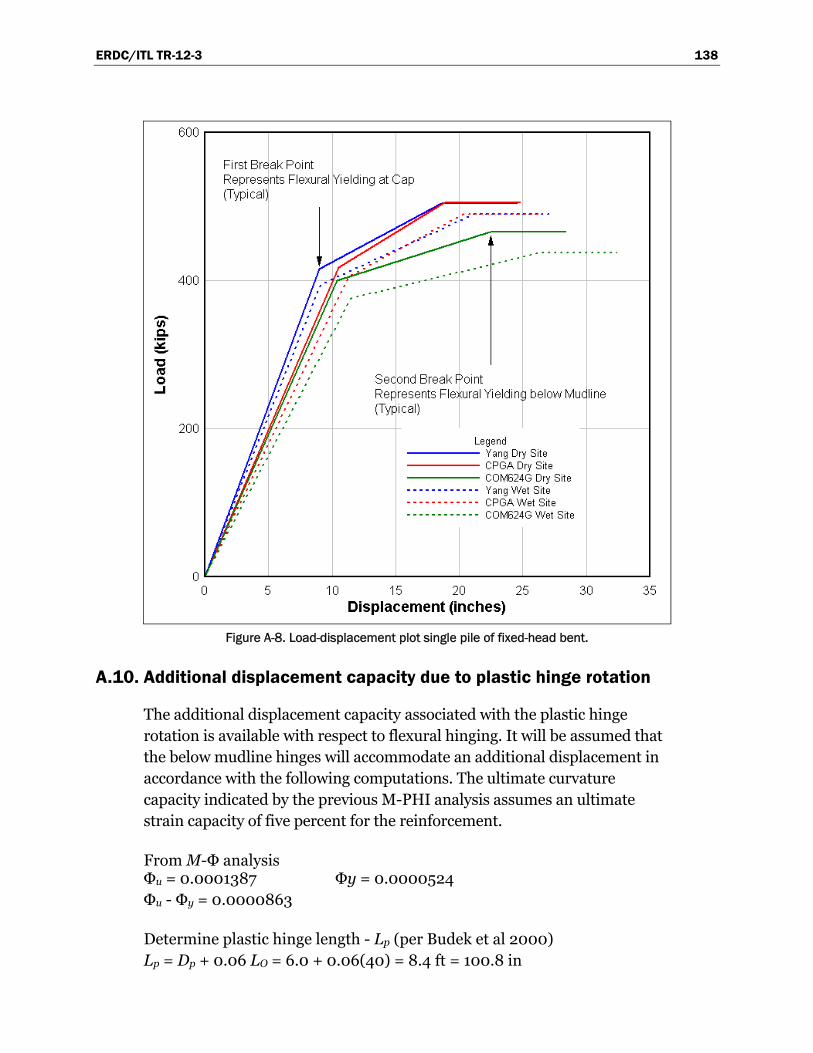
ERDC/ITL TR-12-3 138
Figure A-8. Load-displacement plot single pile of fixed-head bent.
A.10. Additional displacement capacity due to plastic hinge rotation
The additional displacement capacity associated with the plastic hinge rotation is available with respect to flexural hinging. It will be assumed that the below mudline hinges will accommodate an additional displacement in accordance with the following computations. The ultimate curvature capacity indicated by the previous M-PHI analysis assumes an ultimate strain capacity of five percent for the reinforcement.
From M-Φ analysis Φu = 0.0001387 Φy = 0.0000524 Φu - Φy = 0.0000863
Determine plastic hinge length - Lp (per Budek et al 2000) Lp = Dp + 0.06 LO = 6.0 + 0.06(40) = 8.4 ft = 100.8 in
ERDC/ITL TR-12-3 139
Determine plastic hinge rotational capacity – θ θ = (Φu - Φy) Lp = 0.0000863 (100.8) = 0.0087 rads
Determine additional displacement at top of pile due to plastic rotation ΔP = (Φu - Φy) Lp (LO + aT) = 0.0087 [40 + 1.8 (9.851) = 0.50 ft ≈ 6 in.
Figure A.8 shows this additional displacement capacity of the piling for the three methods of analysis.
A.8. Discussion of results from three pushover analyses
In terms of load-displacement plots, Figure A.8 shows that similar results are provided by all three methods of analysis with respect to dry and wet sites. It is surmised that the COM624G analysis provides less potential energy (PE) capacity (i.e., area under the load versus deformation curve) because the nonlinearity of the soil springs near the mudline provide significantly less in the way of soil resistance that do linear elastic springs. Also the COM624 analysis includes pile deformations due to P•Δ effects which may influence results when compared with Yang (1966) and Saul (1968) CPGA analyses.

ERDC/ITL TR-12-3 140
Appendix B: Pushover analysis for batter-pile bent system
B.1. Bent geometry and analytical model used in the pushover analysis
The pipe pile bent of Figure B-1 is examined by pushover analysis to determine its load-displacement characteristics. The Saul (1968), CPGA analytical model used in the analysis is shown in Figure B-2.1 The pipe pile bent is comprised of 24-in. diameter concrete-filled pipe piles. Load-displacement plots will be determined by pushover analysis for pinned-head and fixed-head conditions.
Figure B-1. Pipe pile approach wall.
1 Pile numbers are reported in Figure B-2.
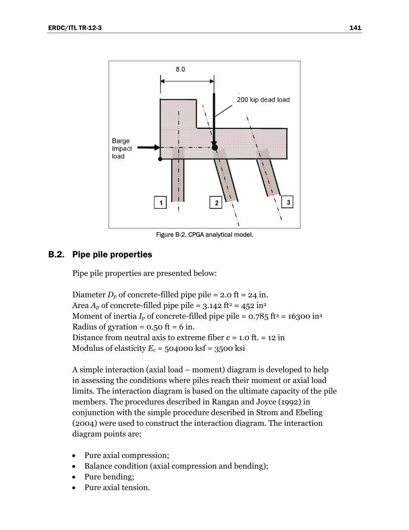
ERDC/ITL TR-12-3 141
Figure B-2. CPGA analytical model.
B.2. Pipe pile properties
Pipe pile properties are presented below:
Diameter Dp of concrete-filled pipe pile = 2.0 ft = 24 in. Area Ap of concrete-filled pipe pile = 3.142 ft2 = 452 in2 Moment of inertia Ip of concrete-filled pipe pile = 0.785 ft4 = 16300 in4 Radius of gyration = 0.50 ft = 6 in. Distance from neutral axis to extreme fiber c = 1.0 ft. = 12 in Modulus of elasticity Ec = 504000 ksf = 3500 ksi
A simple interaction (axial load – moment) diagram is developed to help in assessing the conditions where piles reach their moment or axial load limits. The interaction diagram is based on the ultimate capacity of the pile members. The procedures described in Rangan and Joyce (1992) in conjunction with the simple procedure described in Strom and Ebeling (2004) were used to construct the interaction diagram. The interaction diagram points are:
Pure axial compression; Balance condition (axial compression and bending); Pure bending; Pure axial tension.

ERDC/ITL TR-12-3 142
The value for pure axial compression is based only on the compressive strength of the concrete. The 0.25-in. thick steel pipe casing was not included in this calculation. The value for pure axial tension is based only on the tensile strength of the steel pipe. Balance point and pure moment conditions assumes the contribution only of the concrete in compression on the compressive side of the neutral axis and contribution only of the steel in tension on the tensile side of the neutral axis.
The interaction diagram for a 24-in. diameter concrete-filled pipe pile is presented in Figure B-3.
The interaction diagram assumes that the pipe piles in axial compression fail as a result of the materials (i.e., concrete and steel) reaching their ultimate capacities, rather than by buckling. However buckling computa-tions will be needed to assure that this is the case. If buckling loads are less than the ultimate axial compressive loads predicted by the interaction diagram, then the buckling loads are to be used in the pushover analysis.
Figure B-3. Simple interaction diagram for 24-in. diameter pipe pile.

ERDC/ITL TR-12-3 143
Piles are generally founded in soils that will not allow them to develop their ultimate capacities. It is up to the engineer performing the pushover analysis to consider axial load limitations imposed by the foundation materials. This example also considers pile axial capacities that are limited by side friction and tip resistance provided by the soil foundation.
B.3. Soil properties
A sand foundation with a stiffness that varies linearly with depth is investigated. The coefficient of subgrade reaction (nh) is assumed to be 50 pci. This value for nh is corresponds to Terzaghi’s (1955) “recommended” value for a moist medium-dense sand and within the scatter considering nh values cited in other technical literature (e.g., Davisson, 1970). There is no water table present in this case (i.e., a “dry” site).
The axial capacity based on soil limitations are 250 kips for piles in tension and 1000 kips for piles in compression.
Relative stiffness factor (T):
.c p
h
E IT
n= =5 5 4 ft
B.4. Buckling evaluation
Buckling loads for the concrete-filled pipe piles are determined using methods described in Yang (1996). Figures B-4 and B-5, after Figures 3 and 9 of Yang (1966), are provided for use in the analysis.
The coefficient of free standing length m is equal to the free standing length Lo divided by the relative stiffness factor T, or m = Lo÷ T = 24 ÷ 5.4 = 4.45.
The critical buckling load assuming no translation can be determined using Figure B-4 (after Figure 3 in Yang, 1966).
For pinned-top non-translating pile cap for Figure B-4, the coefficient of critical buckling strength G is equal to 0.026 and the Euler critical buckling load is:
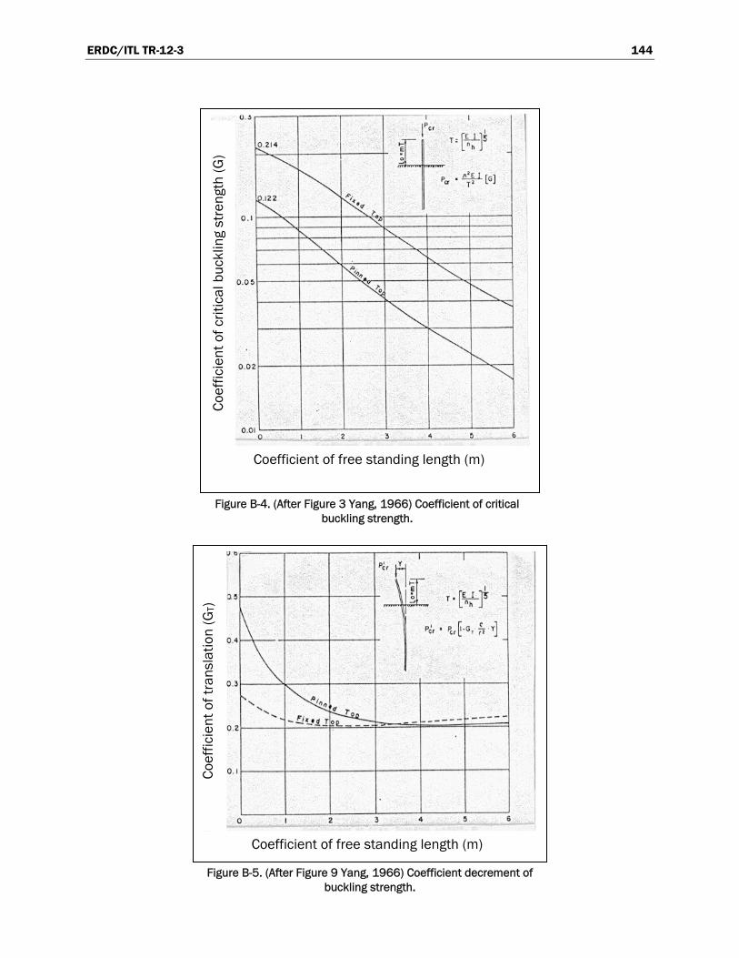
ERDC/ITL TR-12-3 144
Figure B-4. (After Figure 3 Yang, 1966) Coefficient of critical
buckling strength.
Figure B-5. (After Figure 9 Yang, 1966) Coefficient decrement of
buckling strength.
Coefficient of free standing length (m)
Coef
ficie
nt o
f crit
ical
buc
klin
g st
reng
th (G
)
Coefficient of free standing length (m)
Coef
ficie
nt o
f tra
nsla
tion
(GT)

ERDC/ITL TR-12-3 145
[ ]c pCR
π E IP G
T= =
2
2 3847 kips
For fixed-top non-translating pile cap from Figure B-4, the coefficient of critical buckling strength G is equal to 0.056 and the Euler critical buckling load is:
[ ]c pCR
π E IP G
T= =
2
2 7509 kips
The critical buckling load with translation can be determined using Figure B-5 (after Figure 9 of Yang, 1966). Entering Figure B-5 with a coefficient of free standing length (m) equal to 4.45, the coefficient of translation (GT) is approximately equal to 0.21 for both pinned-head and fixed-head piles. The critical buckling load assuming a translation (PCRΔ) is:
Δ ΔCR CR T
cP P G
r
é æ ö ù÷ç= -ê ú÷ç ÷çè øê úë û21 (B.1)
It is desirable for the pushover analysis to have the critical buckling load for various lateral displacements when performing a pushover analysis. This has been accomplished with the aid of MathCAD (1998) for pinned-head piles (Table B-1) and fixed-head piles (Table B-2).
B.5. Pushover analysis for pinned-head condition – dry site
The first pushover analysis is performed for a pinned-head condition at a dry site using Saul’s (1968) method and the CPGA software. The results are summarized in this section. The first incremental analysis was run using an axial stiffness modifier (C33) for the embedded portion of the pile with a value of 1.00 for compression piles and 0.50 for tension piles where:
Δ
Cδ
=33 (B.2)
where:
ΔPLAE
= (B.3)

ERDC/ITL TR-12-3 146
Table B-1. Euler critical buckling load – translating pile top – pinned head condition.
This assumes that the pile is supported at its tip with all axial load (P) transferred to the tip and:
δ = actual displacement of the pile under axial load (P)
This is a crude approximation of axial stiffness used to illustrate the pushover method. The actual value of the stiffness modifier (C33) should be determined by appropriate analytical t-z models and/or pile load tests. To obtain the maximum moment below the mudline it is necessary to include a PMAXMOM data line where:
p
TPMAXMOM
H=
é ùë û (B.4)
Euler critical buckling load - Translating pile top
G T 0.21 Figure 9, Reference 1Pinned top
rI p
A p
0.5
r 0.5 ft c 1.0 ft
3 in 4 in 14 in
P cr ( ) P cr 1 G Tc
r2 x ( )
P cr ( )
2.754·10 3
2.51·10 3
2.266·10 3
2.022·10 3
1.778·10 3
1.534·10 3
1.29·10 3
1.046·10 3
801.897
557.842
313.786
69.73
kip x ( )
3
4
5
6
7
8
9
10
11
12
13
14
in

ERDC/ITL TR-12-3 147
Table B-2. Euler critical buckling load – translating pile top – fixed head condition.
And (Hp), the coefficient of horizontal load for pinned-head conditions, is obtained from Figure B-6 (after Figure 7 of Yang, 1966) and is equal to 0.20.
Therefore:
.
.p
TPMAXMOM
H= = =
é ùë û
5 427
0 20 ft = 324 in.
The “ALLOW” and “UNSP” data lines for CPGA do not represent actual allowable loads and buckling loads but were included only to obtain pile force and displacement results.
Euler critical buckling load - Translating pile top
G T 0.21 Figure 9, Reference 1Fixed top
rI p
A p
0.5
r 0.5 ft c 1.0 ft
3 in 4 in 14 in
P cr ( ) P cr 1 G Tc
r2 x ( )
P cr ( )
5.932·10 3
5.407·10 3
4.881·10 3
4.355·10 3
3.83·10 3
3.304·10 3
2.778·10 3
2.253·10 3
1.727·10 3
1.202·10 3
675.846
150.188
kip x ( )
3
4
5
6
7
8
9
10
11
12
13
14
in

ERDC/ITL TR-12-3 148
Figure B-6. (After Figure 7 Yang, 1966) Coefficient of horizontal load
capacity.
For the first increment of lateral loading, a trial and error process is used to determine the lateral load driving Pile #3 to its axial tensile capacity of 250 kips. This is accomplished with a lateral load of 88 kips. CPGA input and output for this loading increment is presented below.
By trial and error pushover investigations, it can be shown that the next failure mechanism will occur due to flexural yielding of the piles below the mudline. This will be followed by buckling of Pile 2 followed by buckling of Pile 1 as load is shifted from Pile 2 to Pile 1. In the next CPGA run, a low stiffness modifier (C33 = 0.0001) is given to Pile 3 to eliminate its ability to attract axial load. This amounts to releasing Pile 3 in its axial direction since it has reached 250 kips of axial tensile capacity.
Coefficient of free standing length (m)
Coef
ficie
nt o
f hor
izon
tal l
oad
(H)
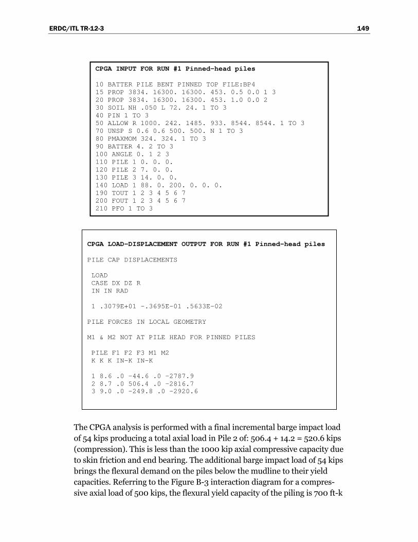
ERDC/ITL TR-12-3 149
The CPGA analysis is performed with a final incremental barge impact load of 54 kips producing a total axial load in Pile 2 of: 506.4 + 14.2 = 520.6 kips (compression). This is less than the 1000 kip axial compressive capacity due to skin friction and end bearing. The additional barge impact load of 54 kips brings the flexural demand on the piles below the mudline to their yield capacities. Referring to the Figure B-3 interaction diagram for a compres-sive axial load of 500 kips, the flexural yield capacity of the piling is 700 ft-k
CPGA LOAD-DISPLACEMENT OUTPUT FOR RUN #1 Pinned-head piles PILE CAP DISPLACEMENTS LOAD CASE DX DZ R IN IN RAD 1 .3079E+01 -.3695E-01 .5633E-02 PILE FORCES IN LOCAL GEOMETRY M1 & M2 NOT AT PILE HEAD FOR PINNED PILES PILE F1 F2 F3 M1 M2 K K K IN-K IN-K 1 8.6 .0 -44.6 .0 -2787.9 2 8.7 .0 506.4 .0 -2816.7 3 9.0 .0 -249.8 .0 -2920.6
CPGA INPUT FOR RUN #1 Pinned-head piles 10 BATTER PILE BENT PINNED TOP FILE:BP4 15 PROP 3834. 16300. 16300. 453. 0.5 0.0 1 3 20 PROP 3834. 16300. 16300. 453. 1.0 0.0 2 30 SOIL NH .050 L 72. 24. 1 TO 3 40 PIN 1 TO 3 50 ALLOW R 1000. 242. 1485. 933. 8544. 8544. 1 TO 3 70 UNSP S 0.6 0.6 500. 500. N 1 TO 3 80 PMAXMOM 324. 324. 1 TO 3 90 BATTER 4. 2 TO 3 100 ANGLE 0. 1 2 3 110 PILE 1 0. 0. 0. 120 PILE 2 7. 0. 0. 130 PILE 3 14. 0. 0. 140 LOAD 1 88. 0. 200. 0. 0. 0. 190 TOUT 1 2 3 4 5 6 7 200 FOUT 1 2 3 4 5 6 7 210 PFO 1 TO 3

ERDC/ITL TR-12-3 150
(8400 in-k) and the flexural demand on Pile #2 is 2817 in-k + 5524 in-k = 8341 in-k. This occurs at a total lateral displacement of 3.1 + 6.0 = 9.1 in. Referring to previous buckling calculations, an axial compressive load of 558 kip with 12.0 in. of lateral displacement will induce buckling. Therefore when subjected to an additional 3-in. of lateral displacement, buckling of Pile #2 is expected to be followed by buckling of Pile #3. It should be noted that CPGA does not have the capability to introduce below mudline flexural hinges and therefore it will be assumed for the purpose of constructing the load-deformation curve that the stiffness of the system remains unchanged between the points below mudline where flexural hinging develops and buckling takes place.
A load-displacement plot for the pinned-head bent at a dry site is presented in Figure B-8 that is located at the end of this Appendix. This figure summarizes the resulting load displacement curves from this and three other CPGA analyses that will be discussed subsequently for pinned-head and fixed-head conditions at dry and wet sand sites. These other three pushover analyses will be summarized prior to discussing the resulting pushover load-displacement curves so that comparisons can be made among the results four analyses.
CPGA INPUT FOR RUN #2 Pinned-head piles 10 CANTILEVER BATTER PILE BENT FILE:BP5 15 PROP 3834. 16300. 16300. 453. 0.0001 0.0 3 20 PROP 3834. 16300. 16300. 453. 1.0 0.0 1 2 30 SOIL NH .047 L 72. 24. 1 TO 3 40 PIN 1 TO 3 50 ALLOW R 1000. 242. 1485. 933. 8544. 8544. 1 TO 3 70 UNSP S 0.6 0.6 500. 500. N 1 TO 3 80 PMAXMOM 324. 324. 1 TO 14 90 BATTER 4. 2 TO 3 100 ANGLE 0. 1 2 3 110 PILE 1 0. 0. 0. 120 PILE 2 7. 0. 0. 130 PILE 3 14. 0. 0. 140 LOAD 1 54. 0. 200. 0. 0. 0. 190 TOUT 1 2 3 4 5 6 7 200 FOUT 1 2 3 4 5 6 7 210 PFO 1 TO 3

ERDC/ITL TR-12-3 151
B.6. Pushover analysis for fixed-head condition – dry site
This section summarizes a second pushover analysis conducted for a fixed-head condition at a dry site using the CPGA software. The first incremental analysis was run using an axial stiffness modifier (C33) for the embedded portion of the pile with a value of 1.00 for compression piles and 0.50 for tension piles. This is a crude approximation of axial stiffness used to illustrate the pushover method. The actual value of the stiffness modifier (C33) should be determined by appropriate analytical t-z models and/or pile load tests. To obtain the maximum moment below the mudline it is necessary to include a FUNSMOM data line where:
O
f
L aTTFUNSMOM
H
+= +
é ùë û 2 (B.5)
where (Hf), the coefficient of horizontal load for fixed-head conditions, is obtained from Figure B-6 (after Figure 7 of Yang, 1966) and is equal to 0.47, and:
LO = free standing length = 24 ft a = coefficient of effective embedment obtained from Figure B-7
for “fixed top translating” = 1.7
CPGA LOAD-DISPLACEMENT OUTPUT FOR RUN #2 Pinned-head piles PILE CAP DISPLACEMENTS LOAD CASE DX DZ R IN IN RAD 1 .5986E+01 .9708E-01 .1889E-01 PILE FORCES IN LOCAL GEOMETRY PILE F1 F2 F3 M1 M2 K K K IN-K IN-K 1 16.5 .0 195.2 .0 -5360.6 2 17.0 .0 14.2 .0 -5524.0 3 18.1 .0 -.5 .0 -5868.6

ERDC/ITL TR-12-3 152
Figure B-7. (After Figure 2 Yang, 1966) Effective embedment of pile at
buckling.
Therefore:
( ). ..
..
O
f
L aTTFUNSMOM
H
++= + = + =
é ùë û
24 1 7 5 45 428 1
2 0 47 2 ft = 337 in.
As before, the “ALLOW” and “UNSP” data lines for CPGA do not represent actual allowable loads and buckling loads but were included only to obtain pile force and displacement results.
For the first increment of lateral loading, a trial and error process is used to determine the lateral load causing the pile to reach their moment capacities at the pile-to-pile cap connection. This is accomplished with a lateral load of 180 kips. CPGA input and output for this loading increment is presented below.
Coefficient of free standing length (m)
Coef
ficie
nt o
f eff
ectiv
e em
bedm
ent (
a)

ERDC/ITL TR-12-3 153
Figure B-8. Load – displacement plot for pipe pile system.
Displacement (inches)
Late
ral L
oad
(kip
s)
0 2 4 6 8 10 12 140
50
100
150
200
250
300
350
Pile to pile capmoment capacity reached
Pile 3 yields in axial tension
Flexural plastic hinges developin piles below mudline
Pile 2 bucklesfollowed by Pile 3
Pile 3 yields in axial tension
Flexural plastic hinges developin piles below the mudline
Pile 2 bucklesfollowed by Pile 1
CPGA INPUT FOR RUN #1 Fixed-head piles 10 BATTER PILE BENT FIXED TOP FILE:BF4 15 PROP 3834. 16300. 16300. 453. 0.5 0.0 1 3 20 PROP 3834. 16300. 16300. 453. 1.0 0.0 2 30 SOIL NH .050 L 72. 24. 1 2 3 40 FIX 1 TO 3 50 ALLOW R 1000. 242. 1485. 933. 8544. 8544. 1 2 3 70 UNSP S 0.6 0.6 1000. 1000. N 1 2 3 80 FUNSMOM 337. 337. 1 3 85 FUNSMOM 337. 337. 2 90 BATTER 4. 2 TO 3 100 ANGLE 0. 1 2 3 110 PILE 1 0. 0. 0. 120 PILE 2 7. 0. 0. 130 PILE 3 14. 0. 0. 140 LOAD 1 180. 0. 200. 0. 0. 0. 190 TOUT 1 2 3 4 5 6 7 200 FOUT 1 2 3 4 5 6 7 210 PFO 1 TO 3

ERDC/ITL TR-12-3 154
For the second increment of lateral loading, a trial and error process is used to determine the lateral load causing pile #3 to reach its tensile load capacity (250 k). This occurs with a lateral load increase of 64 kips. The pile to pile cap connection is changed from fix to pin to capture the yielding that occurred in Run #1.
CPGA INPUT FOR RUN #2 Fixed-head piles 10 BATTER PILE BENT FIXED TOP FILE:BF5 15 PROP 3834. 16300. 16300. 453. 0.5 0.0 1 3 20 PROP 3834. 16300. 16300. 453. 1.0 0.0 2 30 SOIL NH .050 L 72. 24. 1 TO 3 40 PIN 1 TO 3 50 ALLOW R 1000. 242. 1485. 933. 8544. 8544. 1 TO 3 70 UNSP S 0.6 0.6 500. 500. N 1 TO 3 80 PMAXMOM 324. 324. 1 TO 3 90 BATTER 4. 2 TO 3 100 ANGLE 0. 1 2 3 110 PILE 1 0. 0. 0. 120 PILE 2 7. 0. 0. 130 PILE 3 14. 0. 0. 140 LOAD 1 64. 0. 200. 0. 0. 0. 190 TOUT 1 2 3 4 5 6 7 200 FOUT 1 2 3 4 5 6 7 210 PFO 1 TO 3
CPGA LOAD-DISPLACEMENT OUTPUT FOR RUN #1 Fixed-head piles PILE CAP DISPLACEMENTS LOAD CASE DX DY DZ RX RY RZ IN IN IN RAD RAD RAD 1 .2309E+01 .0000E+00 -.1013E+00 .0000E+00 .3155E-02 .0000E+00 PILE FORCES IN LOCAL GEOMETRY PILE F1 F2 F3 M1 M2 K K K IN-K IN-K 1 32.1 .0 -122.1 .0 7002.7 FUNSMOM .0 -3817.5 2 32.3 .0 411.6 .0 7046.6 FUNSMOM .0 -3846.5 3 33.0 .0 -63.2 .0 7188.6 FUNSMOM .0 -3940.4

ERDC/ITL TR-12-3 155
By trial and error pushover investigations it can be seen that next failure mechanism will occur due to flexural yielding of the piles below the mud-line. This will be followed by buckling of Pile 2 followed by buckling of Pile 1 as load is shifted from Pile 2 to Pile 1. In the next CPGA run, a low stiffness modifier (C33 = 0.0001) is given to Pile 3 to eliminate its ability to attract axial load. This amounts to releasing Pile 3 in its axial direction since it has reached 250 kips of axial tensile capacity.
The CPGA analysis is performed with a final incremental barge impact load of 22 kips producing a total axial load in Pile 2 of: 411.6 + 376.7 + 5.8 = 794.1 kips (compression). This is less than the 1000 kips axial compressive capacity due to skin friction and end bearing. The additional barge impact load of 22 kips brings the flexural demand on the piles below the mudline to their yield capacities. Referring to the Figure B-3 interaction diagram for a compressive axial load of 800 kips, the flexural yield capacity of the piling is 670 ft-k (8040 in-k) and the flexural demand on Pile #2 is 3846 in-k + 1937 in-k + 2246 in-k = 8029 in-k indicating demand is approximately equal to capacity. This occurs at a total lateral displacement of 2.3+ 2.1 + 2.4 = 6.8 in. Referring to previous buckling calculations, an axial compressive load of 800 kips at about 12.5 in. of lateral displacement will cause buckling. Therefore when subjected to an additional 6-in. of lateral displacement, buckling of Pile #2 is expected to be followed by buckling of Pile #3. It
CPGA LOAD-DISPLACEMENT OUTPUT FOR RUN #2 Fixed-head piles PILE CAP DISPLACEMENTS LOAD CASE DX DZ R IN IN RAD 1 .2121E+01 .1493E-01 .4192E-02 PILE FORCES IN LOCAL GEOMETRY PILE F1 F2 F3 M1 M2 K K K IN-K IN-K 1 5.9 .0 18.0 .0 -1920.8 2 6.0 .0 376.7 .0 -1937.50 3 6.2 .0 -186.0 .0 -2014.8
Pile #3 has a tensile load of 63.2 k from Run #1 and 186.0 k from Run #2 giving a total axial tensile load of 249.2 k ≈ 250 k. tensile capacity reached.

ERDC/ITL TR-12-3 156
should be noted that CPGA does not have the capability to introduce below mudline flexural hinges; therefore, it will be assumed, for the purpose of constructing the load-deformation curve, that the stiffness of the system remains unchanged between the points below mudline where flexural hinging develops and buckling takes place.
A load-displacement plot for the fixed-head bent at a dry site is presented in Figure B-8.
CPGA OUTPUT FOR RUN #3 Fixed-head piles PILE CAP DISPLACEMENTS LOAD CASE DX DZ R IN IN RAD 1 .2407E+01 .9850E-01 .9300E-02 PILE FORCES IN LOCAL GEOMETRY PILE F1 F2 F3 M1 M2 K K K IN-K IN-K 1 6.7 .0 198.0 .0 -2179.2 2 6.9 .0 5.8 .0 -2245.7 3 7.4 .0 -.2 .0 -2398.8
CPGA INPUT FOR RUN #3 Fixed-head piles 10 BATTER PILE BENT FIXED TOP FILE:BF6 15 PROP 3834. 16300. 16300. 453. 1.0 0.0 1 2 20 PROP 3834. 16300. 16300. 453. 0.0001 0.0 3 30 SOIL NH .050 L 72. 24. 1 TO 3 40 PIN 1 TO 3 50 ALLOW R 1000. 242. 1485. 933. 8544. 8544. 1 TO 3 70 UNSP S 0.6 0.6 500. 500. N 1 TO 3 80 PMAXMOM 324. 324. 1 TO 3 90 BATTER 4. 2 TO 3 100 ANGLE 0. 1 2 3 110 PILE 1 0. 0. 0. 120 PILE 2 7. 0. 0. 130 PILE 3 14. 0. 0. 140 LOAD 1 22. 0. 200. 0. 0. 0. 190 TOUT 1 2 3 4 5 6 7 200 FOUT 1 2 3 4 5 6 7 210 PFO 1 TO 3

ERDC/ITL TR-12-3 157
B.7. Submerged site
A submerged sand foundation with a stiffness that varies linearly with depth is investigated. The coefficient of subgrade reaction (nh) is assumed to be 30 pci. This value for nh is corresponds to Terzaghi’s (1955) “recommended” value for a submerged medium-dense sand per Table 3-2 of Chapter 3. This is sometimes referred to as a “wet” site in this report.
The axial capacity based on soil limitations are 250 kips for piles in tension and 1000 kips for piles in compression.
Relative stiffness factor (T):
.c p
h
E IT
n= =5 6 0 ft
B.8. Buckling evaluation
Buckling loads for the concrete-filled pipe piles are determined using methods described in Yang (1996). Figures B-4 and B-5, after Figures 3 and 9 of Yang (1966), are provided for use in the analysis.
The coefficient of free standing length m is equal to the free standing length Lo divided by the relative stiffness factor T, or m = Lo÷ T = 24 ÷ 6.0 = 4.0.
Assuming no translation, the critical buckling load can be determined using Figure B-4 (after Figure 3 in Yang, 1966).
For pinned-top non-translating pile cap from Figure B-4, the coefficient of critical buckling strength (G) is equal to 0.030 and the Euler critical buckling load is:
[ ]c pCR
π E IP G
T= =
2
2 3256 kips
For fixed-top non-translating pile cap from Figure B-4, the coefficient of critical buckling strength (G) is equal to 0.062 and the Euler critical buckling load is:

ERDC/ITL TR-12-3 158
[ ]c pCR
π E IP G
T= =
2
2 6728 kips
The critical buckling load with translation can be determined using Figure B-5 (after Figure 9 of Yang, 1966). Entering Figure B-5 with a coeffi-cient of free standing length (m) equal to 4.0, the coefficient of translation (GT) is approximately equal to 0.20 for both pinned-head and fixed-head piles. Assuming a translation (PCRΔ), the critical buckling load is:
Δ ΔCR CR T
cP P G
r
é æ ö ù÷ç= -ê ú÷ç ÷çè øê úë û21 (B.6)
It is desirable for the pushover analysis to have the critical buckling load for various lateral displacements when performing a pushover analysis. This has been accomplished with the aid of MathCAD (1998) for pinned-head piles (Table B-3) and fixed-head piles (Table B-4).
B.9. Pushover analysis for pinned-head condition – wet site
This section summarizes a third pushover analysis conducted for a pinned-head condition at a wet site using Saul’s (1968) method and the CPGA software. The first incremental analysis was run using an axial stiffness modifier (C33) for the embedded portion of the pile with a value of 1.00 for compression piles and 0.50 for tension piles where:
Δ
Cδ
=33 (B.7)
where:
ΔPLAE
= (B.8)
This assumes that the pile is supported at its tip with all axial load (P) transferred to the tip and:
δ = actual displacement of the pile under axial load (P)

ERDC/ITL TR-12-3 159
Table B-3. Euler critical buckling load – translating pile top – pinned head condition.
Euler critical buckling load - Translating pile top
GT 0.20 Figure 9, Reference 1Pinned top
rI p
A p
0.5
r 0.5 ft c 1.0 ft
3 in 4 in 14 in
P cr ( ) P cr 1 GTc
r2 x ( )
P cr ( )
2.605·10 3
2.387·10 3
2.17·10 3
1.953·10 3
1.736·10 3
1.519·10 3
1.302·10 3
1.085·10 3
868.176
651.132
434.088
217.044
kip x ( )
3
4
5
6
7
8
9
10
11
12
13
14
in
This is a crude approximation of axial stiffness used to illustrate the pushover method. The actual value of the stiffness modifier (C33) should be determined by appropriate analytical t-z models and/or pile load tests. To obtain the maximum moment below the mudline it is necessary to include a PMAXMOM data line where:
p
TPMAXMOM
H=
é ùë û (B.9)
where (Hp), the coefficient of horizontal load for pinned-head conditions, is obtained from Figure B-6 (after Figure 7 of Yang, 1966) and is equal to 0.21.

ERDC/ITL TR-12-3 160
Table B-4. Euler critical buckling load – translating pile top – fixed head condition.
Euler critical buckling load - Translating pile top
GT 0.20 Figure 9, Reference 1Fixed top
rI p
A p
0.5
r 0.5 ft c 1.0 ft
3 in 4 in 14 in
P cr ( ) P cr 1 GTc
r2 x ( )
P cr ( )
5.383·10 3
4.934·10 3
4.486·10 3
4.037·10 3
3.588·10 3
3.14·10 3
2.691·10 3
2.243·10 3
1.794·10 3
1.346·10 3
897.115
448.557
kip x ( )
3
4
5
6
7
8
9
10
11
12
13
14
in
Therefore:
.
..p
TPMAXMOM
H= = =
é ùë û
6 028 57
0 21 ft = 343 in.
The “ALLOW” and “UNSP” data lines for CPGA do not represent actual allowable loads and buckling loads but were included only to obtain pile force and displacement results.
For the first increment of lateral loading, a trial and error process is used to determine the lateral load driving Pile #3 to its axial tensile capacity of 250 kips. This is accomplished with a lateral load of 88 kips. CPGA input and output for this loading increment is presented below.

ERDC/ITL TR-12-3 161
***************************************************************** PILE CAP DISPLACEMENTS LOAD CASE DX DZ R IN IN RAD 1 .3096E+01 -.3789E-01 .5660E-02 ***************************************************************** PILE FORCES IN LOCAL GEOMETRY LOAD CASE - 1 PILE F1 F2 F3 M1 M2 K K K IN-K IN-K 1 7.9 .0 -45.7 .0 -2700.6 2 8.0 .0 508.5 .0 -2728.53 3 8.2 .0 -251.2 .0 -2829.1 *****************************************************************
By trial and error pushover investigations, it can be shown that the next failure mechanism will occur due to flexural yielding of the piles below the
CPGA INPUT FOR RUN #1 Pinned-head piles 10 BATTER PILE BENT PINNED TOP FILE:BP8 15 PROP 3834. 16300. 16300. 453. 0.5 0.0 1 3 20 PROP 3834. 16300. 16300. 453. 1.0 0.0 2 30 SOIL NH .030 L 72. 24. 1 TO 3 40 PIN 1 TO 3 50 ALLOW R 1000. 242. 1485. 933. 8544. 8544. 1 TO 3 70 UNSP S 0.6 0.6 500. 500. N 1 TO 3 80 PMAXMOM 343. 343. 1 TO 3 90 BATTER 4. 2 TO 3 100 ANGLE 0. 1 2 3 110 PILE 1 0. 0. 0. 120 PILE 2 7. 0. 0. 130 PILE 3 14. 0. 0. 140 LOAD 1 88. 0. 200. 0. 0. 0. 190 TOUT 1 2 3 4 5 6 7 200 FOUT 1 2 3 4 5 6 7 210 PFO 1 TO 3
Horizontal displacement equals 3.1 inch
Pile #3 reaches its axial load capacity of 250 kips
Maximum moments below the mudline

ERDC/ITL TR-12-3 162
mudline. This will be followed by buckling of Pile 2 followed by buckling of Pile 1 as load is shifted from Pile 2 to Pile 1. In the next CPGA run, a low stiffness modifier (C33 = 0.0001) is given to Pile 3 to eliminate its ability to attract axial load. This amounts to releasing Pile 3 in its axial direction since it has reached 250 kips of axial tensile capacity.
The CPGA analysis is performed with a final incremental barge impact load of 52 kips producing a total axial load in Pile 2 of: 508.5 + 13.8 = 522.3 kip (compression). This is less than the 1000 kips axial compressive capacity due to skin friction and end bearing. The additional barge impact load of 52 kips brings the flexural demand on the piles below the mudline to their yield capacities. Referring to the Figure B-3 interaction diagram for a compressive axial load of 500 kips, the flexural yield capacity of the piling is 700 ft-k (8400 in-k) and the flexural demand on Pile #2 is 2728.5 in-k + 5630.7 in-k = 8359.2 in-k. This occurs at a total lateral displacement of 3.1 + 6.3 = 9.4 in. Referring to previous buckling calculations, an axial compressive load of 560 kips with 12.0 in. of lateral displacement will induce buckling. Therefore when subjected to an additional 3-in. of lateral displacement, buckling of Pile #2 is expected to be followed by buckling of Pile #3. It should be noted that CPGA does not have the capability to introduce below mudline flexural hinges and therefore it will be assumed for the purpose of constructing the load-deformation curve that the stiffness of the system remains unchanged between the points below mudline where flexural hinging develops and buckling takes place.
CPGA INPUT FOR RUN #2 Pinned-head piles 10 CANTILEVER BATTER PILE BENT FILE:BP5 15 PROP 3834. 16300. 16300. 453. 0.0001 0.0 3 20 PROP 3834. 16300. 16300. 453. 1.0 0.0 1 2 30 SOIL NH .030 L 72. 24. 1 TO 3 40 PIN 1 TO 3 50 ALLOW R 1000. 242. 1485. 933. 8544. 8544. 1 TO 3 70 UNSP S 0.6 0.6 500. 500. N 1 TO 3 80 PMAXMOM 343. 343. 1 TO 14 90 BATTER 4. 2 TO 3 100 ANGLE 0. 1 2 3 110 PILE 1 0. 0. 0. 120 PILE 2 7. 0. 0. 130 PILE 3 14. 0. 0. 140 LOAD 1 52. 0. 200. 0. 0. 0. 190 TOUT 1 2 3 4 5 6 7 200 FOUT 1 2 3 4 5 6 7 210 PFO 1 TO 3

ERDC/ITL TR-12-3 163
***************************************************************** PILE CAP DISPLACEMENTS LOAD CASE DX DZ R IN IN RAD 1 .6265E+01 .9716E-01 .1972E-01 ***************************************************************** PILE FORCES IN LOCAL GEOMETRY LOAD CASE - 1 PILE F1 F2 F3 M1 M2 K K K IN-K IN-K 1 15.9 .0 195.3 .0 -5464.0 2 16.4 .0 13.8 .0 -5630.7 3 17.4 .0 -.5 .0 -5981.1 *****************************************************************
A load-displacement plot for the pinned-head bent at the wet site is presented in Figure B-8.
B.10. Pushover analysis for fixed-head condition – wet site
This section summarizes a fourth pushover analysis conducted for a fixed-head condition at a wet site using Saul’s (1968) method and the CPGA software. The first incremental analysis was run using an axial stiffness modifier (C33) for the embedded portion of the pile with a value of 1.00 for compression piles and 0.50 for tension piles. This is a crude approximation of axial stiffness used to illustrate the pushover method. The actual value of the stiffness modifier (C33) should be determined by appropriate analytical t-z models and/or pile load tests. To obtain the maximum moment below the mudline it is necessary to include a FUNSMOM data line where:
O
f
L aTTFUNSMOM
H
+= +
é ùë û 2 (B.10)
Where (Hf), the coefficient of horizontal load for fixed-head conditions, is obtained from Figure B-6 (after Figure 7 of Yang, 1966) and is equal to 0.52, and:

ERDC/ITL TR-12-3 164
LO = free standing length = 24 ft a = coefficient of effective embedment obtained from Figure B-7
for “fixed top translating” = 1.75
Therefore:
( ). ..
..
O
f
L aTTFUNSMOM
H
++= + = + =
é ùë û
24 1 7 6 06 028 6
2 0 52 2 ft = 344 in.
As before, the “ALLOW” and “UNSP” data lines for CPGA do not represent actual allowable loads and buckling loads but were included only to obtain pile force and displacement results.
For the first increment of lateral loading, a trial and error process is used to determine the lateral load causing the pile to reach their moment capacities at the pile to pile cap connection. This is accomplished with a lateral load of 180 kips. CPGA input and output for this loading increment is presented below.
***************************************************************** PILE CAP DISPLACEMENTS LOAD
CPGA INPUT FOR RUN #1 Fixed-head piles 10 BATTER PILE BENT FIXED TOP FILE:BF7 15 PROP 3834. 16300. 16300. 453. 0.5 0.0 1 3 20 PROP 3834. 16300. 16300. 453. 1.0 0.0 2 30 SOIL NH .030 L 72. 24. 1 2 3 40 FIX 1 TO 3 50 ALLOW R 1000. 242. 1485. 933. 8544. 8544. 1 2 3 70 UNSP S 0.6 0.6 1000. 1000. N 1 2 3 80 FUNSMOM 344. 344. 1 3 85 FUNSMOM 344. 344. 2 90 BATTER 4. 2 TO 3 100 ANGLE 0. 1 2 3 110 PILE 1 0. 0. 0. 120 PILE 2 7. 0. 0. 130 PILE 3 14. 0. 0. 140 LOAD 1 180. 0. 200. 0. 0. 0. 190 TOUT 1 2 3 4 5 6 7 200 FOUT 1 2 3 4 5 6 7 210 PFO 1 TO 3

ERDC/ITL TR-12-3 165
CASE DX DY DZ IN IN IN 1 .2462E+01 .0000E+00 -.1102E+00 ***************************************************************** PILE FORCES IN LOCAL GEOMETRY LOAD CASE - 1 PILE F1 F2 F3 M1 M2 K K K IN-K IN-K 1 31.2 .0 -132.9 .0 7045.0 FUNSMOM .0 -3699.8 2 31.5 .0 431.9 .0 7090.5 FUNSMOM .0 -3729.1 3 32.1 .0 -72.9 .0 7232.5 FUNSMOM .0 -3820.5 *********************************************************************
For the second increment of lateral loading, a trial and error process is used to determine the lateral load causing pile #3 to reach its tensile load capacity (250 k). This occurs with a lateral load increase of 70 kips. The pile to pile cap connection is changed from fix to pin to capture the yielding that occurred in Run #1.
By trial and error pushover investigations, it can be seen that next failure mechanism will occur due to flexural yielding of the piles below the mud-line. This will be followed by buckling of Pile 2 followed by buckling of Pile 1 as the load is shifted from Pile 2 to Pile 1. In the next CPGA run a low stiffness modifier (C33 = 0.0001) is given to Pile 3 to eliminate its ability to attract axial load. This amounts to releasing Pile 3 in its axial direction since it has reached 250 kips of axial tensile capacity.
The CPGA analysis is performed with a final incremental barge impact load of 22 kips producing a total axial load in Pile 2 of: 431.9 + 419.3 + 5.9 = 857.1 kips (compression). This is less than the 1000 kips axial compressive capacity due to skin friction and bearing. The additional barge impact load of 22 kips brings the flexural demand on the piles below the mudline to
From Figure B-3 (interaction diagram) for a tensile load of 122 kips the moment capacity ≈ 610 ft-k (7330 in-k). Therefore moment demand ≈ moment capacity at pile to pile cap connection.

ERDC/ITL TR-12-3 166
***************************************************************** PILE CAP DISPLACEMENTS LOAD CASE DX DZ R IN IN RAD 1 .2437E+01 -.2179E-02 .4668E-02 ***************************************************************** PILE FORCES IN LOCAL GEOMETRY LOAD CASE - 1 PILE F1 F2 F3 M1 M2 K K K IN-K IN-K 1 6.2 .0 -2.6 .0 -2131.9 2 6.3 .0 419.3 .0 -2151.91 3 6.5 .0 -207.2 .0 -2235.1 *****************************************************************
their yield capacities. Referring to the Figure B-3 interaction diagram for a compressive axial load of 800 kips, the flexural yield capacity of the piling is 675 ft-k (8100 in-k) and the flexural demand on Pile #2 is 3729 in-k + 2152 in-k + 2385 in-k = 8266 in-k which indicates that the demand is slightly greater than the capacity. This occurs at a total lateral displacement of 2.5 + 2.4 + 2.6 = 7.5 in. Referring to previous buckling calculations an axial compressive load of 857 kips at about 13 in. of lateral displacement will
CPGA INPUT FOR RUN #2 Fixed-head piles 10 BATTER PILE BENT FIXED TOP FILE:BF8 15 PROP 3834. 16300. 16300. 453. 0.5 0.0 1 3 20 PROP 3834. 16300. 16300. 453. 1.0 0.0 2 30 SOIL NH .030 L 72. 24. 1 TO 3 40 PIN 1 TO 3 50 ALLOW R 1000. 242. 1485. 933. 8544. 8544. 1 TO 3 70 UNSP S 0.6 0.6 500. 500. N 1 TO 3 80 PMAXMOM 344. 344. 1 TO 3 90 BATTER 4. 2 TO 3 100 ANGLE 0. 1 2 3 110 PILE 1 0. 0. 0. 120 PILE 2 7. 0. 0. 130 PILE 3 14. 0. 0. 140 LOAD 1 70. 0. 200. 0. 0. 0. 190 TOUT 1 2 3 4 5 6 7 200 FOUT 1 2 3 4 5 6 7 210 PFO 1 TO 3
Pile #3 has a tensile load of 32.1 k from Run #1 and 207.2 k from Run #2 giving a total axial tensile load of 239.3 k ≈ 250 k. tensile capacity reached.

ERDC/ITL TR-12-3 167
cause buckling. Therefore, when subjected to an additional 5.5-in. of lateral displacement, buckling of Pile #2 is expected to be followed by buckling of Pile #3. It should be noted that CPGA does not have the capability to introduce below mudline flexural hinges and therefore it will be assumed for the purpose of constructing the load-deformation curve that the stiffness of the system remains unchanged between the points below mudline where flexural hinging develops and buckling takes place.
***************************************************************** PILE CAP DISPLACEMENTS LOAD CASE DX DZ R IN IN RAD 1 .2645E+01 .9849E-01 .9010E-02 ***************************************************************** PILE FORCES IN LOCAL GEOMETRY LOAD CASE - 1 PILE F1 F2 F3 M1 M2 K K K IN-K IN-K 1 6.7 .0 198.0 .0 -2314.0 2 6.9 .0 5.9 .0 -2384.5 3 7.4 .0 -.2 .0 -2545.1 *****************************************************************
CPGA INPUT FOR RUN #3 Fixed-head piles 10 BATTER PILE BENT FIXED TOP FILE:BF6 15 PROP 3834. 16300. 16300. 453. 1.0 0.0 1 2 20 PROP 3834. 16300. 16300. 453. 0.0001 0.0 3 30 SOIL NH .030 L 72. 24. 1 TO 3 40 PIN 1 TO 3 50 ALLOW R 1000. 242. 1485. 933. 8544. 8544. 1 TO 3 70 UNSP S 0.6 0.6 500. 500. N 1 TO 3 80 PMAXMOM 344. 344. 1 TO 3 90 BATTER 4. 2 TO 3 100 ANGLE 0. 1 2 3 110 PILE 1 0. 0. 0. 120 PILE 2 7. 0. 0. 130 PILE 3 14. 0. 0. 140 LOAD 1 22. 0. 200. 0. 0. 0. 190 TOUT 1 2 3 4 5 6 7 200 FOUT 1 2 3 4 5 6 7 210 PFO 1 TO 3

ERDC/ITL TR-12-3 168
A load-displacement plot for the fixed-head bent at the wet site is presented in Figure B-8. The resulting structural system versus displacement plots characterize the potential energy capacity of the particular batter pile bent being analyzed. The pushover results for four systems are shown in this figure.
In Figure B-8 the load-displacement results by the Saul (1968) method for a dry site (nh = 50 pci) are represented by solid line and those for a submerged or wet site (nh = 30 pci) by dashed lines. Yang (1966) and COM624G methods cannot be used for batter pile systems because they are only applicable to single vertical pile analysis. The methods can be used for systems comprised of multiple vertical piles since a single pile from the system can be analyzed and the load-displacement results for the entire system derived based on the behavior of that single pile.
The load-displacement curves for the fixed-head pile system have four break points designating places where pile or soil yielding occurs. The number of yield points and the type of yielding will be pile bent and foundation dependent. For the particular pile bent – foundation system investigated, the first break point (one with lowest displacement demand) occurs when flexural yielding takes place at the pile to pile cap connection. The second break point occurs when Pile Number 3 yields in axial tension (a foundation to pile transfer mechanism).1 The third break point occurs when flexural yielding takes place in the piles below the mudline. The fourth break point occurs when Pile Number 2 buckles. Pile buckling quickly results in pile bent system failure with little reserve potential energy capacity in the system.
There is little difference between the behaviors of submerged (wet) sites and dry sites, recognizing that lock approach wall bent systems will always be submerged. With batter pile systems, the resistance to lateral load comes principally from pile axial stiffness and not from flexural stiffness as is the case with vertical pile systems. Therefore changes in lateral subgrade resistance (e.g, nh) have little effect on system load-displacement behavior.
It can easily be recognized from Figure B-2 that the fixed-head system has much greater potential energy capacity than the free-head system. The free-head system does not possess the added lateral force resistance
1 Recall pile numbers are reported in Figure B-2.

ERDC/ITL TR-12-3 169
provided by rigid pile to pile cap connections (which is the first break point for the fixed-head system).
The information contained in this appendix illustrates the pushover analysis for a pinned-head and fixed-head batter pile bent using the Corps computer program CPGA (X0080) for wet and dry sites (i.e., nh = 30 pci and 50 pci, respectively). Note that potential failure mechanisms and the sequence in which they form will likely be different for other batter-pile bent system groups and pile configurations.

ERDC/ITL TR-12-3 170
Appendix C: GROUP 7 Pushover analysis for batter-pile bent system
C.1. Bent geometry and analytical model used in the pushover analysis
An additional pushover analysis on the pipe pile bent shown in Figure C-1 was performed to determine its load-displacement characteristics. This pushover analysis utilized the computer program GROUP 7 by (Reese et al. 2006). Group 7 analyzes the behavior of pile groups using either a two-dimensional (2-D) or three-dimensional (3-D) model. The program has options to approximate the nonlinear response of the soil, in the form of t-z and q-w curves for axial loading and p-y curves for lateral loading. The results of the analyses using GROUP 7 were compared to the results using the CASE computer program CPGA (Appendix B). The GROUP 7 analytical model used in the analysis is shown in Figure C-2. The pipe pile bent is comprised of 24-in. diameter concrete-filled pipe piles. Load-displacement plots were determined by pushover analysis for pinned-head boundary conditions.
Figure C-1. Three pipe pile approach wall.

ERDC/ITL TR-12-3 171
Figure C-2. GROUP 7 analytical model of the pipe pile approach wall.
When discussing pile performance in this appendix, the three piles shown in Figure C-1 are referred to by pile number (from left to right). Pile number 1 is the vertical pipe pile closest to the front impact point on the deck while pile number 3 is the batter pile farthest from the point of impact.
C.2. Pipe pile properties
The same pipe pile properties used in the Appendix B CPGA analysis were used in the GROUP 7 analysis and are presented below:
Diameter Dp of concrete-filled pipe pile = 2.0 ft = 24 in. Area Ap of concrete-filled pipe pile = 3.142 ft2 = 452 in2 Moment of inertia Ip of concrete-filled pipe pile = 0.785 ft4 = 16300 in4 Radius of gyration = 0.50 ft = 6 in. Distance from neutral axis to extreme fiber c = 1.0 ft. = 12 in Modulus of elasticity Ec = 504000 ksf = 3500 ksi
As noted in Appendix B, piles are generally founded in soils that will not allow them to develop their ultimate capacities for the design loads. It is up to the engineer performing the pushover analysis to consider axial load limitations imposed by the foundation materials. This pushover analysis example considers pile axial capacities that are limited by side friction and tip resistance provided by the soil foundation.

ERDC/ITL TR-12-3 172
C.3. Soil properties
In the CPGA analyses discussed in Appendix B, the soil supporting the piles was moist medium-dense sand with an estimated value of the coefficient of horizontal subgrade reaction (nh) equal to 50 pci. This particular sand site is referred to as the dry site in this report since no water table is included. The axial capacity based on soil limitations were 250 kips for piles in tension and 1000 kips for piles in compression. These same values for nh and axial capacities were utilized in the Group 7 analyses to provide a direct comparison of results. However, for the Group 7 analyses, a parametric study was conducted to obtain plausible input values of unit side resistance (fmax) and unit point resistance (qmax) required for computing nonlinear response curves due to axial loading while maintaining numerical stability.
C.3. Pushover analysis results comparison for pinned-head boundary condition
The primary objective of performing the additional pushover analysis using Group 7 was to ascertain the effects that accounting for the nonlinear soil behavior (both axial and lateral) have on the overall force-displacement response of this pipe pile approach wall system. Also, this additional pushover analysis provides a direct comparison of results between Group 7 and CPGA (results given in Appendix B). Figure C-3 shows a typical Group 7 input file used in the analyses. As mentioned above, a series of pushover analyses using Group 7 were conducted to obtain a plausible range in input values of unit side resistance (fmax) and unit point resistance (qmax) required for computing nonlinear response curves due to axial loading that results in a completed analysis which is numerically stable. These analysis results were compared to the results of a pushover analysis using CPGA. Table C-1 shows a summary of the CPGA and Group 7 pushover analysis results. Recall, in the Group 7 analyses the value of the coefficient of horizontal subgrade reaction (nh) equal 50 pci was utilized. This was the same nh value used in the CPGA analyses.
An initial Group 7 analysis was performed assuming a linear variation in fmax that ranged from zero lbs/in2 at the ground surface to 11.0 lbs/in2 at the pile tip and qmax equal 700 lbs/in2 at the pile tip. These values were based Figures 76 and 77 from Mosher (1984)1 for the WES criteria for sands having an internal friction angle () equal to 35 degrees and without pile
1 These two figures are provided in Appendix D.

ERDC/ITL TR-12-3 173
test results being adjusted due to residual stresses. To obtain values for fmax and qmax, the ratio of pile embedment length to pile diameter is required. With the length of pile embedment (L) equal to 48 ft and a diameter (D) equal to 2 ft, the equation results in a ratio of L/D equal to 24. The average standard error for the unadjusted pile test results was approximately 25 percent compared to 32 percent for the adjusted field test values. However, this analysis did not converge to a solution and thus a parameter study was performed. Observe in Table C-1, that there was only one Group 7 analysis that obtained a complete solution, identified as Run Set 8. This analysis had a unit side resistance (fmax) equal to 20 lbs/in2 at pile tip and unit point resistance (qmax) equal to 500 lbs/in2 at the pile tip. This Group 7 analysis did not indicate that a failure mechanism had formed while the GPGA analysis indicated a tension failure had formed for pile number 3 (i.e., the batter pile farthest from the load). Recall from Appendix B, the axial capacity of 250 kips for piles in tension (i.e., full mobilization of the pile-to-soil interface shearing resistance along the length of the pile). The Group 7 analysis of pile number 3 computed an axial load of 31.3 kips in tension compared to 249.8 kips in tension computed in the CPGA analysis.
Figure C-3. Group 7 Input File used in the pushover analysis (for Run Set 8).
GROUP 7 INPUT FOR Pinned-head pilesRun #1 Pinned-head piles GROUP7.0.11 1 0 0 1 0 0 0 0 0 2 0 0 1 1 0 100 100 1.0000000E-05 1.0000000E-05 1.0000000E+00 1.0000000E+00 2.0000000E+05 8.8000000E+04 0.0000000E+00 0.0000000E+00 0.0000000E+00 0.0000000E+00 3 1 1 1 0 0 0 -84 0 288 0 1 1 1 0 0 0 0 0.245 288 0 1 1 1 0 0 0 84 0.245 288 0 1 1 1 50 864 3500000 1 0 864 24 452 16300 0 1 2 2 0 1 4 288 1200 50 288 0.637 1200 0.637 288 0 35 0 0 0 0 1200 0 35 0 20 500 0 1.0000000E+00

ERDC/ITL TR-12-3 174
Table C-1. CPGA and Group 7 pushover analysis comparisons.
Note: Column 5 in Table C-1 reports the ultimate unit side resistance, fmax, at pile tip. All analyses assume a zero value for fmax at top of ground. A linear variation is assumed for fmax with depth between these two points (i.e., ground surface and pile tip) in the Group 7 analyses.
The Group 7 parametric study also indicated there was no consistent failure mechanism development. The failure mechanisms changed between tension and bearing failures for relatively small changes in input values of fmax and qmax at intermediate stages of the analyses; e.g., Run Sets 3 and 4. The reported failure mechanism is a bearing failure for pile number 3 for Run Set 3 with qmax equal to 450 lbs/in2, For Run Set 4 with qmax equal to 500 lbs/in2 the reported failure mechanism is a tension
Run Set Program
BC at Pile
Headnh
(pci)
Unit Side (fmax)
(lbs/in2)
Unit Point (qmax)
(lbs/in2)Analysis
CompletedFailure Mode
and Pile #
Cap Displacement
(in.)Axial Load
(kips)
CPGA Pinned 50 N/A N/A Yes Tension / 3 3.1 -249.8GROUP 7 Pinned 5 2.5 350 No N/A N/A N/A
CPGA Pinned 50 N/A N/A Yes Tension / 3 3.1 -249.8GROUP 7 Pinned 50 2.5 400 No Bearing / 3 N/A N/A
CPGA Pinned 50 N/A N/A Yes Tension / 3 3.1 -249.8GROUP 7 Pinned 50 2.5 450 No Bearing / 3 N/A N/A
CPGA Pinned 50 N/A N/A Yes Tension / 3 3.1 -249.8GROUP 7 Pinned 50 2.5 500 No Tension / 3 N/A N/A
CPGA Pinned 50 N/A N/A Yes Tension / 3 3.1 -249.8GROUP 7 Pinned 50 5 500 No Tension / 3 N/A N/A
CPGA Pinned 50 N/A N/A Yes Tension / 3 3.1 -249.8GROUP 7 Pinned 5 10 500 No N/A N/A N/A
CPGA Pinned 50 N/A N/A Yes Tension / 3 3.1 -249.8GROUP 7 Pinned 50 15 50 No Tension 2&3 N/A N/A
CPGA Pinned 50 N/A N/A Yes Tension / 3 3.1 -249.8GROUP 7 Pinned 50 20 500 Yes N/A 4.1 -31.3
CPGA Pinned 50 N/A N/A Yes Tension / 3 3.1 -249.8GROUP 7 Pinned 50 10 600 No Bearing / 3 N/A N/A
CPGA Pinned 50 N/A N/A Yes Tension / 3 3.1 -249.8GROUP 7 Pinned 5 15 600 No Bearing / 3 N/A N/A
CPGA Pinned 50 N/A N/A Yes Tension / 3 3.1 -249.8GROUP 7 Pinned 50 2.5 400 No Bearing / 3 N/A N/A
CPGA Pinned 50 N/A N/A Yes Tension / 3 3.1 -249.8GROUP 7 Pinned 50 2.5 450 No Bearing / 3 N/A N/A
CPGA Pinned 50 N/A N/A Yes Tension / 3 3.1 -249.8GROUP 7 Pinned 50 2.5 500 No Tension / 3 N/A N/A
CPGA Pinned 50 N/A N/A Yes Tension / 3 3.1 -249.8GROUP 7 Pinned 50 5 500 No Tension / 3 N/A N/A
12
13
14
8
9
10
11
4
5
6
7
Resistance
1
2
3

ERDC/ITL TR-12-3 175
failure of pile number 3. Again, from the parametric study using Group 7, there was only one case that resulted in a complete analysis; Run Set 8. This indicates that modeling of nonlinear axial response in Group 7 is sensitive to user defined input values for fmax and qmax. An example of this convergence sensitivity is Run Set 8 which converged to a solution with (fmax) equal to 20 lbs/in2 (at pile tip) and unit point resistance (qmax) equal to 500 lbs/in2, compared to Run Set 9 which did not converge to a solution with (fmax) equal to 10 lbs/in2 (at pile tip) and unit point resistance (qmax) equal to 600 lbs/in2.
A comparison plot of the lateral force-displacement responses from pushover analyses using both Group 7 and CPGA for Run Set 8 is shown in Figure C-4. The computed displacement responses from Group 7 closely mirrored those from CPGA for applied lateral loads greater than 80 kips and less than 140 kips. The Group 7 results show nonlinear force-displacement response for lateral loading less than 80 kips compared to linear response from the CPGA results, indicating that “softer” springs are being used at this lower load level in the CPGA push-over analysis.
Figure C-4. GROUP 7 and CPGA push-over results for the of the three pipe pile approach wall
(Run Set 8).
In Run Set 8, the computed cap displacement for the Group 7 analysis was 3.5 in. for an intermediate loading of 88 kips analysis stage without the development of a failure mechanism. The corresponding CPGA analysis computed a cap displacement of 3.1 in. when pile number 3 yields in
Load Displacement Plot for pipe pile system
0
20
40
60
80
100
120
140
160
180
0 2 4 6 8 10 12 14
Displacement (inches)
Fo
rce
(Kip
s)
Group 7
CPGA
Pile 3 yields in axial tension
Flexural plastic hinges develop in pile below mudline
Pile 2 buckles followed by Pile 1
Load Displacement Plot for pipe pile system
0
20
40
60
80
100
120
140
160
180
0 2 4 6 8 10 12 14
Displacement (inches)
Fo
rce
(Kip
s)
Group 7
CPGA
Pile 3 yields in axial tension
Flexural plastic hinges develop in pile below mudline
Pile 2 buckles followed by Pile 1

ERDC/ITL TR-12-3 176
tension (i.e., the development of the first “mechanism”) as identified in Figure C-4. The development of other failure mechanisms in other parts of the pile group and bent system are identified in this figure during the course of the CPGA push-over analysis. No failure mechanisms were identified during the course of the continued Group 7 push-over analysis for Run Set 8.
In this study, the Group 7 analyses did not provide critical insight on the formation of failure mechanisms as was indicated by results from the CPGA push-over analyses. The authors of this report speculate that this is a direct result of all nonlinear response features contained within the Group 7 analysis package. In addition, the Group 7 results for horizontal loading less than 80 kips indicate the soil springs in the CPGA analysis to be “soft.”

ERDC/ITL TR-12-3 177
Appendix D: Skin friction and tip capacities of piles
D.1. Introduction
The skin friction capacity and limiting tip resistance of a pile founded in sand or in clay may be determined using one of the procedures outlined in this appendix.
D.2. Skin friction and tip capacities of piles according to EM 1110-2-2906
The skin friction and tip capacity of a pile founded in different materials (i.e., sand or clay) may be determined using one of the relationships given in this section. This material was first presented in Chapter 4 of EM 1110-2-2906 (1991).
D.2.1 Pile capacity
Pile capacities should be computed by an experienced designer that is thoroughly familiar with the various types of piles, how piles behave when loaded, and the soil conditions that exist at the site.
D.2.1.1 Axial pile capacity
The axial capacity of a pile may be represented by the following formula:
ult s tQ Q Q= + (D.1)
s s sQ f A= (D.2)
t tQ qA= (D.3)
where:
Qult = ultimate pile capacity; Qs = shaft resistance of the pile due to skin friction; Qt = tip resistance of the pile due to end bearing; fs = average unit skin resistance;

ERDC/ITL TR-12-3 178
As = surface area of the shaft in contact with the soil; q = unit tip-bearing capacity; At = effective (gross) area of the tip of the pile in contact with the
soil.
1. Piles in cohesionless soil.
a. Skin Friction. For design purposes, the skin friction of piles in sand increase linearly to an assumed critical depth (Dc) and then remain constant below that depth. The critical depth varies between 10 to 20 pile diameters or widths (B), depending on the relative density of the sand. The critical depth is assumed as:
Dc = 10B for loose sands Dc = 15B for medium dense sands Dc = 20B for dense sands
The unit skin friction acting on the pile shaft may be determined by the following equations:
tans vf Kσ δ¢= (D.4)
v cσ γD for D D¢ = < (D.5)
v c cσ γD for D D¢ = ³ (D.6)
s s sQ f A= (D.7)
where:
K = lateral earth pressure coefficient (Kc for compression piles and Kt for tension piles);
v ’ = effective overburden pressure; = angle of friction between the soil and the pile; ’ = effective unit weight of soil; D = depth along the pile at which the effective overburden pressure
is calculated.
Values of are given in Table D-1.

ERDC/ITL TR-12-3 179
Table D-1. Values of
Values of
Pile Material
Steel 0.67 to 0.83
Concrete 0.90 to 1.0
Timber 0.80 to 1.0
Values of K for piles in compression (Kc) and piles in tension (Kt) are given in Table D-2. Table D-1 and Table D-2 present ranges of values of and K based upon experience in various soil deposits. These values should be selected for design based upon experience and pile load test. It is not intended that the designer would use the minimum reduction of the angle while using the upper range K values.
Table D-2. Values of K.
Values of K
Soil Type Kc Kt
Sand 1.00 to 2.00 0.50 to 0.70
Silt 1.00 0.50 to 0.70
Clay 1.00 0.70 to 1.00
Note: The above do not apply to piles that are prebored, jetted, or installed with a vibratory hammer. Picking K values at the upper end of the above ranges should be based on local experience. K , , and Nq values back calculated from load tests may be used.
For steel H-piles, As should be taken as the block perimeter of the pile and should be the average friction angles of steel against sand and sand against sand (). It should be noted that Table D-2 is general guidance to be used unless the long-term engineering practice in the area indicates otherwise. Under prediction of soil strength parameters at load test sites have at times produced back-calculated values of K that exceed the values in Table D-2. It has also been found both theoretically and at some test sites that the use of displacement piles produces higher values of K than does the use of nondisplacement piles. Values of K that have been used satisfactorily but with standard soil data in some locations are as follows in Table D-3:

ERDC/ITL TR-12-3 180
Table D-3. Common Values for Corrected K.
Common Values for Corrected K
Soil Type
Displacement Piles Nondisplacement Piles
Compression Tension Compression Tension
Sand 2.00 0.67 1.50 0.50
Silt 1.25 0.50 1.00 0.35
Clay 1.25 0.90 1.00 0.70
Note: Although these values may be commonly used in some areas they should not be used without experience and testing to validate them.
b. End Bearing. For design purposes, the pile-tip bearing capacity can be assumed to increase linearly to a critical depth (Dc) and then remain constant. The same critical depth relationship used for skin friction can be used for end bearing. The unit tip bearing capacity can be determined as follows:
v qq σ N¢= (D.8)
where:
v cσ γD for D D¢ = < (D.9)
v c cσ γD for D D¢ = ³ (D.10)
For steel H-piles At should be taken as the area included within the block perimeter. A curve to obtain the Terzagi and Peck (1967) bearing capacity factor Nq (among values from other theories) is shown in Figure D-1. To use the curve one must obtain measured values of the angle of internal friction () which represents the soil mass.
c. Tension Capacity. The tension capacity of piles in sand can be calcu-lated as follows using the K values for tension from Table D-2:
ult tensionQ Qs= (D.11)
2. Piles in Cohesive Soil

ERDC/ITL TR-12-3 181
Figure D-1. Bearing capacity factor.
a. Skin Friction. Although called skin friction, the resistance is due to the cohesion or adhesion of the clay to the pile shaft.
s af c= (D.12)
ac ac= (D.13)
s s sQ f A= (D.14)
where:
ca = adhesion between the clay and the pile; = adhesion factor; c = undrained shear strength of the clay from a Q test.

ERDC/ITL TR-12-3 182
The values of as a function of the undrained shear are given in Figure D-2a.
Figure D-2. a) Values of versus undrained shear strength b) Values of 12 applicable for
very long piles.
An alternate procedure developed by Semple and Rigden (1984) to obtain values of which is especially applicable for very long piles, is given in Figure D-2b where:
a a a= 1 2 (D.15)
and
sf ac= (D.16)
b. End Bearing. The pile unit-tip bearing capacity for piles in clay can be determined from the following equation:

ERDC/ITL TR-12-3 183
9q c= (D.17)
t tQ A q= (D.18)
However, the movement necessary to develop the tip resistance of piles in clay soils may be several times larger than that required to develop the skin friction resistance.
c. Compression Capacity. By combining the skin friction capacity and the tip bearing capacity, the ultimate compression capacity may be found as follows:
ult s tQ Q Q= + (D.19)
d. Tension Capacity. The tension capacity of piles in clay may be calculated as:
ult sQ Q= (D.20)
e. The pile capacity in normally consolidated clays (cohesive soils) should also be computed in the long-term S shear strength case. That is, develop a S case shear strength trend as discussed previously and proceed as if the soil is drained. The computational method is identical to that presented for piles in granular soils, and to present the computational methodology would be redundant. It should be noted however that the shear strengths in clays in the S case are assumed to be > 0 and C = 0.
Some commonly used S case shear strengths in alluvial soils are as follows in Table D-4:
Table D-4. S Case shear strength.
S Case Shear Strength
Soil Type Consistency Angle of Internal Friction
Fat clay (CH) Very soft 13° to 17°
Fat clay (CH) Soft 17° to 20°
Fat clay (CH) Medium 20° to 21°
Fat clay (CH) Stiff 21° to 23°
Silt (ML) 25° to 28°
Note: The designer should perform testing and select shear strengths. These general data ranges are from test on specific soils in site specific environments and may not represent the soil in question.

ERDC/ITL TR-12-3 184
3. Piles in Silt.
a. Skin Friction. The skin friction on a pile in silt is a two component resistance to pile movement contributed by the angle of internal friction () and the cohesion (c) acting along the pile shaft. That portion of the resistance contributed by the angle of internal friction () is, as with the sand, limited to a critical depth of (Dc), below which the frictional portion remains constant. The limit depths are stated below. That portion of the resistance contributed by the cohesion may require a limit if it is sufficiently large, see Figures D-2a and b. The shaft resistance may be computed as follows:
tanKγD δ ac+ (D.21)
where (D Dc)
s s sQ A f= (D.22)
where
Qs = capacity due to skin resistance; fs = average unit skin resistance; As = surface area of the pile shaft in contact with soil; K = see Table D-2; = see Figures D-2a and b; D = depth below ground up to limit depth Dc; = limit value for shaft friction angle from Table D-1.
b. End Bearing. The pile tip bearing capacity increases linearly to a critical depth (Dc) and remains constant below that depth. The critical depths are given as follows:
Dc = 10 B for loose silts Dc = 15 B for medium silts Dc = 20 B for dense silts
The unit and bearing capacity may be computed as follows:
’v qq σ N= (D.23)

ERDC/ITL TR-12-3 185
’ forv cσ γD D D= < (D.24)
’ forv c cσ γD D D= ³ (D.25)
t tQ A q= (D.26)
where:
Nq = Terzaghi bearing capacity factor, Figure D-1; v ’ = vertical earth pressure at the tip with limits; At = area of the pile tip, as determined for sands.
c. Compression Capacity. By combining the two incremental contributors, skin friction and end bearing, the ultimate capacity of the soil/pile may be computed as follows:
ult s tQ Q Q= + (D.27)
d. Tension Capacity. The tension capacity is computed by applying the appropriate value of Kt from Table D-2 to the unit skin friction equation above.
ult tensionQ Qs= (D.28)
e. It is recommended that, when designing pile foundations in silty soils, consideration should be given to selecting a very conservative shear strength from classical R shear tests. It is further recom-mended that test piles be considered as a virtual necessity, and the possibility that pile length may have to be increased in the field should be considered.
3. Piles in Layered Soils. Piles are most frequently driven into a layered soil stratigraphy. For this condition, the preceding methods of computation may be used on a layer by layer basis. The end bearing capacity of the pile should be determined from the properties of the layer of soil where the tip is founded. However, when weak or dissimilar layers of soil exist within approximately 5 ft or 8-pile tip diameters, whichever is the larger, of the tip founding elevation the end bearing capacity will be affected. It is necessary to compute this affect and account for it when assigning end bearing capacity. In computing the skin resistance, the contribution of
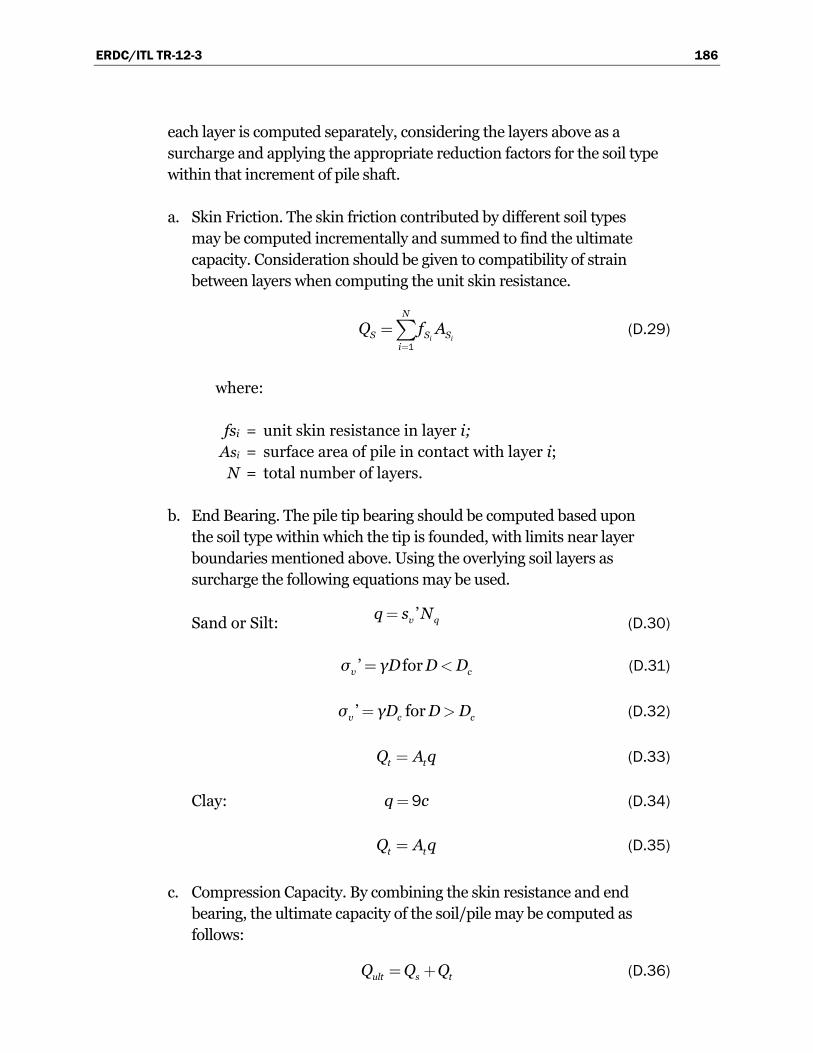
ERDC/ITL TR-12-3 186
each layer is computed separately, considering the layers above as a surcharge and applying the appropriate reduction factors for the soil type within that increment of pile shaft.
a. Skin Friction. The skin friction contributed by different soil types may be computed incrementally and summed to find the ultimate capacity. Consideration should be given to compatibility of strain between layers when computing the unit skin resistance.
i i
N
S S Si
Q f A=
=å1
(D.29)
where:
fsi = unit skin resistance in layer i; Asi = surface area of pile in contact with layer i; N = total number of layers.
b. End Bearing. The pile tip bearing should be computed based upon the soil type within which the tip is founded, with limits near layer boundaries mentioned above. Using the overlying soil layers as surcharge the following equations may be used.
Sand or Silt: ’v qq s N=
(D.30)
’ forv cσ γD D D= < (D.31)
’ forv c cσ γD D D= > (D.32)
t tQ A q= (D.33)
Clay: q c=9 (D.34)
t tQ A q= (D.35)
c. Compression Capacity. By combining the skin resistance and end bearing, the ultimate capacity of the soil/pile may be computed as follows:
ult s tQ Q Q= + (D.36)

ERDC/ITL TR-12-3 187
d. Tension Capacity. The tension capacity may be computed by applying the appropriate values of Kt from Table D-2 as appropriate for granular soils to the incremental computation for each layer and then combining to yield:
ult tensionQ Qs= (D.37)
4. Point Bearing Piles. In some cases, the pile will be driven to refusal upon firm good quality rock. In such cases the capacity of the pile is governed by the structural capacity of the pile or the rock capacity.
D.2.1.2 Pile group capacity
The pile group capacity for piles in cohesionless and cohesive soils is given below.
1. Piles in Cohesionless Soil. The pile group efficiency is defined as:
group
ult
Q
NQ= (D.38)
where:
Qgroup = ultimate capacity of a pile group; N = number of piles in a group;
Qult = ultimate capacity of a single pile.
The ultimate group capacity of driven piles in sand is equal to or greater than the sum of the ultimate capacity of the single piles. Therefore in practice, the ultimate group capacity of driven piles in sand not underlain by a weak layer, should be taken as the sum of the single pile capacities (= 1). For piles jetted into sand, is less than one. For piles underlain by a weak layer, the ultimate group capacity is the smaller of (a) the sum of the single pile ultimate capacities or (b) the capacity of an equivalent pier with the geometry defined by enclosing the pile group Terzagi and Peck (1967). The base strength should be that of the weak layer.
2. Piles in Cohesive Soil. The ultimate group capacity of piles in clay is the smaller of (a) the sum of the single pile ultimate capacities or (b) the

ERDC/ITL TR-12-3 188
capacity of an equivalent pier Terzagi and Peck (1967) . The ultimate group capacity of piles in clay is given by the smaller of the following two equations:
group ultQ NQ= (D.39)
( ) ggroup g g b G G
g g
BDQ B L Dc c L B
B L
é æ öæ öù÷ ÷ç çê ú÷ ÷= + + + +ç ç÷ ÷ç çê ú÷ ÷ç çè øè øë û2 5 1 1
5 5 (D.40)
where:
gc
g g
BDN
B L
æ öæ ö÷ ÷ç ç÷ ÷= + + £ç ç÷ ÷ç ç÷ ÷ç çè øè ø5 1 1 9
5 5 (D.41)
and:
Bg = width of the pile group; Lg = length of the pile group; D = depth of the pile group; ̅ = weighted average of undrained shear strength over the depth
of pile embedment. ̅ should be reduced by from Figure D-2;
cb = undrained shear strength at the base of the pile group.
This equation applies to a rectangular section only. It should be modified for other shapes.
D.3 Skin friction and tip capacities of piles according to Castello
The skin friction capacity of a pile founded in sand may be determined using the procedure recommended by Mosher (1984). Dr. Mosher investigated load-transfer criteria of axially loaded piles in sand. One of the products from his investigation was a pair of charts attributed to the research of Castello (1980) for skin-friction capacity and for pile tip capacity. These charts were identified as Figures 76 and 77 in the Mosher report and are reproduced in Figures D-3 and D-4. Evaluations of the field data made by Mosher (page 159) state that the average standard error of the “unadjusted” values for side resistance is 25 percent. There was a second chart included in the Mosher report that is similar to Figure D-3 but developed by using
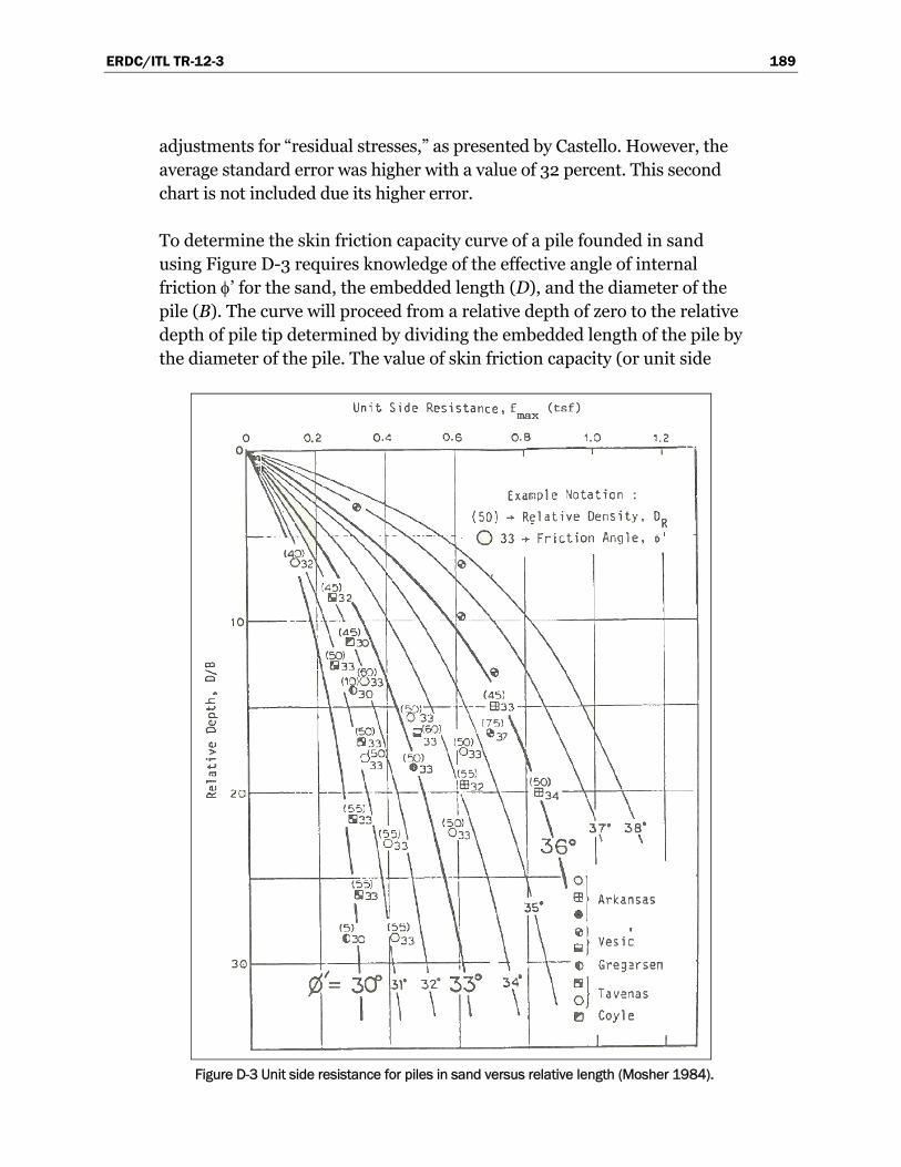
ERDC/ITL TR-12-3 189
adjustments for “residual stresses,” as presented by Castello. However, the average standard error was higher with a value of 32 percent. This second chart is not included due its higher error.
To determine the skin friction capacity curve of a pile founded in sand using Figure D-3 requires knowledge of the effective angle of internal friction ’ for the sand, the embedded length (D), and the diameter of the pile (B). The curve will proceed from a relative depth of zero to the relative depth of pile tip determined by dividing the embedded length of the pile by the diameter of the pile. The value of skin friction capacity (or unit side
Figure D-3 Unit side resistance for piles in sand versus relative length (Mosher 1984).

ERDC/ITL TR-12-3 190
Figure D-4 Unit tip resistance for piles in sand versus relative length (Mosher 1984).
resistance – with units of tsf) for a specified depth of embedment is determined by finding where the current relative depth intersects the curve for the angle ’, which is parabolic with depth. It is possible to approximate this parabolic curve with a piecewise linear definition for the skin friction capacity curve. Interval relative depth values along the pile are determined by dividing the interval depth of embedment by the diameter of the pile. At these regular relative depth intervals, the skin friction capacity can be determined from the figure as described above. The results are more accurate with an increasing number of intervals between the mudline and the total depth of embedment of the pile.

ERDC/ITL TR-12-3 191
To determine the unit tip resistance of a pile founded in sand using Figure D-4 requires knowledge of the effective angle of internal friction ’ for the sand, the embedded length, and the diameter of the pile. The length of pile embedded in sand is normalized by the pile diameter. It is referred to as the “relative depth.” For this “relative depth” and a specified value of ’ the unit tip resistance (in units of tsf) is obtained by intersecting the unit tip resistance value the appropriate curve for ’ in Figure D-4. Thus the unit tip resistance of a pile founded in sand is established.

ERDC/ITL TR-12-3 192
Appendix E: Dynamic Response of Impact Wall Systems
E.1 Introduction
Solution techniques involving modal analysis are often used to perform a dynamic structural analysis for response of flexible approach wall structural systems and/or key flexible system structural features to an impact pulse force time-history. The flexible impact beam response analysis software Impact_Beam (Ebeling et al 2011) is one such example. This appendix describes methods used to establish the dynamic characteristics of (1) drilled-in-place (DIP) bent systems, (2) batter pile (BP) bent systems, and (3) long impact wall beams. Dynamic characteristics of interest are natural periods of vibration and mode shapes. In general, the natural period of vibration is a scalar value defined by the mass and stiffness for a structural member (or system), while mode shapes characterize the natural displaced shape of a structural member (or system) in free vibration. Free vibration means the motion of the structural system without dynamic excitation (i.e., neither external forces nor base or ground motion). Each modal frequency relates back to a value for the natural period of vibration Tn, expressed in units of seconds. As noted by Chopra (1995, page 367-68), each characteristic deflected shape is the natural mode of vibration for a multi-degree-of-freedom (MDOF) system.1 Modal properties are typically used in the dynamic response evaluation of structural systems to a rapidly applied loading such as an earthquake or a pulse force loading (which, by definition, is of short duration). The information contained in this appendix will be used to characterize those modes significantly contributing to the total response of the structural system (always mode number one, likely mode numbers two and three, possible higher modes). This modal information will be of use in the next stage of the developmental effort involving modeling of the dynamic structural response of flexible impact deck structural systems founded on pile groups loaded with a pulse force impact time history. The resulting PC-based software will be referred to as “Impact_Deck”.
An engineering methodology has been developed that allows for the conversion of the momentum normal to the wall (i.e., mass times
1 For the selected natural mode number n, the natural period of vibration Tn of a MDOF system is the
time required for one cycle of the simple harmonic motion in units of seconds.

ERDC/ITL TR-12-3 193
velocitynormal) into a pulse force time history using the impulse-momentum principle (Ebeling et al 2010). The corresponding PC-based software Impact_Force facilitates this conversion process. One method of specifying demand in a dynamic time-history analysis is to apply a pulse force time history as the impact load normal to a user-defined model of the flexible approach wall.
Using one of the simplified structural modal models presented earlier in this report, these features of pulse force time history analysis are briefly described.
E.2 Dynamic characteristics of DIP bents, BP bent systems and long impact wall beams using simplified models
This section describes the use of simplified models of DIP bents, BP bent systems and long impact wall beams to determine the demands due to barge impacts. The simplified dynamic models being used are based on the vibrational properties of (undamped) modal frequencies and mode shapes.
E.2.1 Natural period
The vibrational characteristics of the drilled-in-pile (DIP) and batter pile (BP) bent systems are evaluated along with the vibrational characteristics of a flexible impact wall system spanning between fixed supports such as concrete-filled cells. The analyses contained herein are directed towards the DIP and BP bent systems described in previous chapters.
Impact wall systems when examined by pulse loading techniques require that the natural period Tn of the system (fundamental period) be known since the peak response of the deformable wall system can occur during either forced vibration response or during free vibration response, with the magnitude of the structural response depending on the relationship of the system natural period to the duration of the pulse loading. The bent systems first examined are considered to behave as 2-D systems. In other words, no consideration is given to 3-D impact wall configurations (with 3-D load sharing effects) where rigid supports occur at the longitudinal extremities of the wall. Drilled-in-place and batter-pile bents are flexible and as such permit redistribution of impact load from the bent or bents closest to the point of impact to adjacent bents. Redistribution of impact load is unlikely for large diameter cellular sheet pile supporting systems that are rigid. Using 3-D analytical methods that can capture redistribution effects is

ERDC/ITL TR-12-3 194
therefore required in the final stages of wall design. One approach used in a 3-D analysis process is described at the end of this section.
Following the approach used by Priestley et al. (1996) for bridge piers, the natural period Tn of a DIP or BP bent system can be estimated using Equations E.1 and E.3. When using these equations, it is assumed that one-third of the pile weight is tributary to the pile cap and the remaining pile weight (that below the top one-third) has little effect on the natural period.
( ).
( )C P
n
w wT π
k g
+=
0 332 in seconds (E.1)
where:
wc = Weight of pile cap and hydrodynamic mass tributary to pile bent (kip);
wp = Weight above the mudline of all piles in the bent (kip); k = Lateral stiffness of pile bent system prior to first yield
mechanism (kip/ft); g = Acceleration of gravity (32.2 ft/sec2).
The elastic stiffness (stiffness prior to formation of the first yield mechanism) is used to determine the natural period of vibration. Except for extreme barge impact loadings, the response of pile bents are likely to be near-yield (versus post-yield) for all participating pile under anticipated usual and unusual performance criteria. One of the objectives of this report is to propose Corps performance criteria for the usual, unusual and extreme loadings. Under extreme barge impact loadings, most pile bents (with the exception of those immediately adjacent to the point of barge impact) will likely be at near-yield response levels (and below deformation levels associated with system collapse).
Since pushover analyses will be used as the basis for estimating the load-displacement response for a particular pile bent system, the load and displacement at first yield can be used to determine the natural period of the pile bent system. This can be accomplished by the Rayleigh Equation.
A form of the Raleigh Equation is provided below (Equation E.2). Equation E.2 is in accordance with Equation 23.5 in Paz (1991) and Equation 5-2 of TM 5-809-10-1 (1986). A version of the Raleigh Equation

ERDC/ITL TR-12-3 195
expressed in terms of natural frequency is provided by Equation 9.6, Goyal and Chopra (1989).
N
i ii
n N
i ii
W δT π
g f δ
=
=
=å
å
2
1
1
2 (E.2)
where:
N = Number of concentrated mass points ; Wi = Weight at mass point “i”; I = Displacement at mass point “i”; fi = Force at mass point “i”.
Limited model studies conducted on the two Drilled In Place (DIP) and Batter Pile (BP) flexible approach wall systems shown in the previous chapters indicate that the pile bent can be idealized by a single lumped mass located at the pile cap:
( )
( ).p c
H
w w δT π
g P
+=
1
0 332 (E.3)
where:
δ = Displacement at formation of first yield mechanism; PH1 = Horizontal force creating first yield mechanism.
Recognizing that the stiffness is equal PH1/δ, it can be seen that Equations E.1 and E.3 are equivalent.
In the above equations, the total mass is equal to the impact beam mass tributary to each bent (including hydrodynamic added mass) and one-third the mass of the bent including its hydrodynamic added mass.
The natural period of long impact beams spanning between rigid supports (e.g., concrete filled cells) can be also be estimated through simple formulation. These formulations are provided for end conditions that are fixed against rotation and for end conditions that permit free rotation. The

ERDC/ITL TR-12-3 196
formulations are based on the assumption that the mass (impact beam mass + hydrodynamic added mass) are uniformly distributed along the length of the impact beam.
E.2.2 Single-mode analysis
The two flexible impact wall systems shown in previous chapters were found to be first mode dominant and can be designed or analyzed using single-mode analysis techniques. For analysis purposes, it is necessary to determine if a single-mode analysis will provide suitable results. This generally occurs when the first mode mass participation factor, sometimes referred to as the base shear participation factor is equal to, or greater than, 0.90 and will most likely occur when the first mode mass participation factor is greater than 0.80. Single-mode analysis will become more approximate as the first mode mass participation factor diminishes. A generalized mode shape was developed and is provided for the impact walls supported by a DIP bent system. This generalized mode shape is useful in estimating first mode mass participation. It can also be used to estimate the natural period of vibration although other methods described in the report are generally more applicable. The authors observe that the vibrational characteristics of the various flexible wall systems can be determined using structural software programs with dynamic analysis capability. The SAP analysis program was used to produce the generalized mode shape provided below for the DIP bent system. Generalized mode shapes are used to estimate the generalized mass (m*) at the top of an impact wall bent, Priestly et al. (1996).
This generalized mass (m*) can be expressed using a general deformation model (mode shape) that is representative of the particular type of bent under consideration. The mode shape must have a modal value equal to one at the top of the bent (i.e., point of maximum displacement). The generalized mass equation expressed in terms of a known mass distribution is:
* ( ) ( )H
Cm m x ψ x dx= ò 2
0 (E.4a)
where:
)(xmC = mass as a function of the distance (x) along the vertical axis of
the bent;
)(x = displacement shape function (mode shape) as a function of (x).

ERDC/ITL TR-12-3 197
Expressed in terms of a system where masses are lumped at discrete node points:
*NP npm m φ=å 2 (E.4b)
where:
m NP = mass assigned to a designated nodal point; Φ NP = modal value at a designated nodal point.
The natural period of vibration Tn of the bent system can be approximated by:
*
n
mT π
k= 2 (E.5)
where:
k = stiffness of the bent assuming all mass is concentrated at the top of the bent.
With respect to the earthquake design and evaluation of bridge piers and bents (Priestley et al. 1996), a linear mode shape is often used. This assumes that plastic hinging develops at the base of the bridge piers and therefore the deflected shape will be close to linear. It is likely during extreme barge impact events that only those drilled-in-place or batter-pile bents in close proximity to the point of impact will yield. Since most, if not all, of the bents participating in the response to barge impact will remain elastic, a deflected shape associated with a linear elastic response is assumed.
The vibrational characteristics (e.g., mode shapes and natural periods Tn) of the impact beam spanning between concrete-filled cells can be determined by simple formulations for both simple support conditions and fixed-support conditions. Typically these formulations can be found in Paz (1991), Chopra (1995), et cetera. However they are generally based solely on deformations from flexure. Information is provided to allow shear deformations to be included.

ERDC/ITL TR-12-3 198
E.2.3 DIP bent system
The drilled-in-pile (DIP) bent system is comprised of two drilled-in caissons (piles) that are fixed against rotation at the pile-to pile-cap connection. The bents are spaced at regular intervals along the length of the impact wall. A fixed-head system with its simplified analytical model, generalized mode shape and modal values is illustrated in Figure E-1. The reasonableness of this model was demonstrated by comparisons with more detailed SAP finite element model results.
Figure E-1. Fixed-head bent system -Analytical model and general mode shape.
The simplified analytical model assumes that fixed-head pile bent behavior can be approximated by an equivalent depth to fixity model. The analytical model is a lumped-mass (tributary weight) model and contains five lumped mass locations per pile, two at the pile-to pile-cap connection

ERDC/ITL TR-12-3 199
and with the other eight equally spaced in pairs of two along the free standing length of the piles from the pile cap to the point of fixity (POF). The height (h) of the analytical model is equal to the length above the mudline (LO) plus the length below the mudline to the point of fixity (L).
Use of the generalized mode shape and modal values in the determination of the first mode mass participation factor MPF and natural period of vibration Tn are provided in Figure E-2. The calculations are per the Appendix A example for a fixed-head pile bent that extends 40 ft above the mudline with a length to point of fixity equal to 18 ft giving a total height equal to 58 ft. The cap weight is equal to 1917 kips per bent. The drilled-in-piles weigh 4.2 kips per ft.
Figure E-2. Natural period and mass participation factor - Demonstration calculations.

ERDC/ITL TR-12-3 200
Using the load (836 kip) and displacement (0.874 ft) for the point of first yield from the Appendix A example, by Equation E.3:
( )( )
. . ( ) ..
. ( )c p
nH
w w δT π π s
g P
+ += = =
1
0 33 1917 0 33 336 0 8742 2 1 61
32 2 836
The period provides a good match to that calculated using the generalized mode shape.
The fixed-head drilled-in caisson (pile) system used for the natural period analysis are per the Appendix A example and assumed to contain piles that are 6.0 ft in diameter and reinforced with bundled #14 bars (e.g., see Figure A-4). This system represents the upstream approach wall at Melvin Price Lock and Dam as presented in Figure 10.8 of the Upper Mississippi River -Illinois Waterway System Navigation Study, Locks and Dams 22 and 25, Approach Wall System Design Considerations and Concept Recommendation
The effective stiffness (k) for the fixed-head pile bent system is:
[ ]( )( . ) . , ,EIk
h h h= = =3 3 3
24 504000 63 62 0 2524 192 400 000 kips/ft
where:
h = distance from cap to point of fixity (POF)
It is assumed the practical range of heights (from cap to POF) is from 30 to 90 ft. Using this range in height and Equation E.1, the natural periods of vibration (in height increments of 10 ft) are determined and presented in Table E-1. The weight tributary to the pile cap is assumed to be 2000 kips. This information is intended to provide a general range of natural periods for the DIP bent system.
The natural periods of vibration contained in Table E-1 are based on an effective stiffness equal to 25 percent of the gross stiffness. To obtain natural periods based on gross stiffness, divide the Table E-1 values by 2.
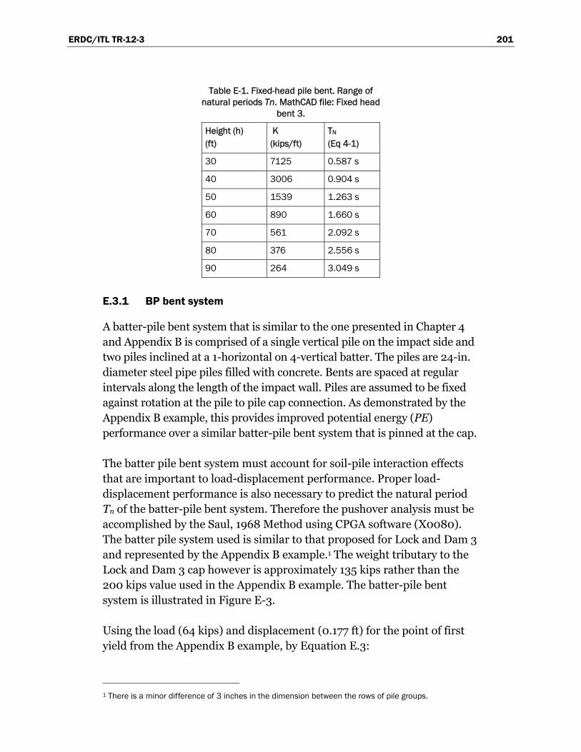
ERDC/ITL TR-12-3 201
Table E-1. Fixed-head pile bent. Range of natural periods Tn. MathCAD file: Fixed head
bent 3.
Height (h) (ft)
K (kips/ft)
TN (Eq 4-1)
30 7125 0.587 s
40 3006 0.904 s
50 1539 1.263 s
60 890 1.660 s
70 561 2.092 s
80 376 2.556 s
90 264 3.049 s
E.3.1 BP bent system
A batter-pile bent system that is similar to the one presented in Chapter 4 and Appendix B is comprised of a single vertical pile on the impact side and two piles inclined at a 1-horizontal on 4-vertical batter. The piles are 24-in. diameter steel pipe piles filled with concrete. Bents are spaced at regular intervals along the length of the impact wall. Piles are assumed to be fixed against rotation at the pile to pile cap connection. As demonstrated by the Appendix B example, this provides improved potential energy (PE) performance over a similar batter-pile bent system that is pinned at the cap.
The batter pile bent system must account for soil-pile interaction effects that are important to load-displacement performance. Proper load-displacement performance is also necessary to predict the natural period Tn of the batter-pile bent system. Therefore the pushover analysis must be accomplished by the Saul, 1968 Method using CPGA software (X0080). The batter pile system used is similar to that proposed for Lock and Dam 3 and represented by the Appendix B example.1 The weight tributary to the Lock and Dam 3 cap however is approximately 135 kips rather than the 200 kips value used in the Appendix B example. The batter-pile bent system is illustrated in Figure E-3.
Using the load (64 kips) and displacement (0.177 ft) for the point of first yield from the Appendix B example, by Equation E.3:
1 There is a minor difference of 3 inches in the dimension between the rows of pile groups.
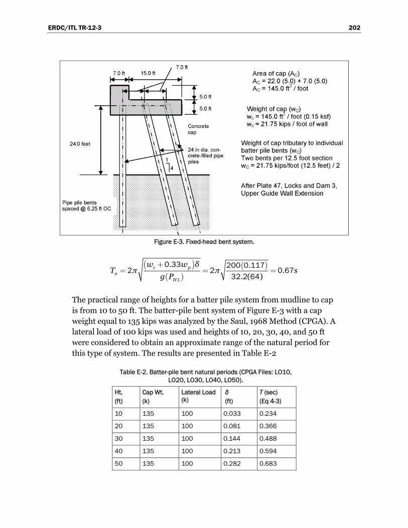
ERDC/ITL TR-12-3 202
Figure E-3. Fixed-head bent system.
( )( )
( ). ..
. ( )c p
nH
w w δT π π s
g P
+= = =
1
0 33 200 0 1172 2 0 67
32 2 64
The practical range of heights for a batter pile system from mudline to cap is from 10 to 50 ft. The batter-pile bent system of Figure E-3 with a cap weight equal to 135 kips was analyzed by the Saul, 1968 Method (CPGA). A lateral load of 100 kips was used and heights of 10, 20, 30, 40, and 50 ft were considered to obtain an approximate range of the natural period for this type of system. The results are presented in Table E-2
Table E-2. Batter-pile bent natural periods (CPGA Files: LO10, LO20, LO30, LO40, LO50).
Ht. (ft)
Cap Wt. (k)
Lateral Load (k)
δ (ft)
T (sec) (Eq 4-3)
10 135 100 0.033 0.234
20 135 100 0.081 0.366
30 135 100 0.144 0.488
40 135 100 0.213 0.594
50 135 100 0.282 0.683

ERDC/ITL TR-12-3 203
4.2.1 Long span beam impact wall
The long span beam impact wall example considered is one of several proposed impact wall systems considered for Lock and Dam 22 (Figure E-4). Only the upstream impact wall is considered since it is likely to sustain higher impact loads than the downstream walls. The upstream wall is comprised of two 9-ft x 9-ft precast-prestressed box sections stacked one on the other and anchored together to form a composite section. A single 9-ft x 9-ft precast-prestressed box section along with the section properties for the composite system is illustrated in Figure E-5.
The mass of the system consists of the wall mass and added hydrodynamic mass as indicated in Figure E-6.
The Westergaard added mass approach is used to approximate hydro-dynamic effects. Calculations for hydrodynamic added weight for the upstream wall under normal pool conditions are provided in Figure E-7.
An assumed normal pool condition is used in this example since it would be overly conservative to couple maximum pool conditions with extreme barge impact loading effects. However, pool conditions consistent with usual, unusual, and extreme loadings should be used for each of the respective
Figure E-4. Proposed impact wall – Lock 22.

ERDC/ITL TR-12-3 204
Figure E-5. Properties of upstream impact wall – Lock 22.
calculations. It should be noted that the resultant of the hydrodynamic mass does not coincide with the center of rigidity for the impact wall and, therefore, some torsional effects will result. These were investigated for this particular wall and found to not alter the systems dynamic characteristics. However, if a skirt is provided on the underside of the wall to improve flow conditions, this will capture additional hydrodynamic mass, possibly making the torsional response a dominant feature and cause the natural period to lengthen thereby changing the impact loading. This applies also to the downstream wall where the added hydrodynamic mass is likely to be significantly greater.

ERDC/ITL TR-12-3 205
Figure E-6. Lock 22 upstream wall – normal pool condition.
Figure E-7. MathCAD calculations for upstream wall.
Many structural dynamics textbooks provide period formulations for beams with uniform mass distribution for conditions where end supports are free to rotate (pinned connection) and fixed against rotation (e.g., Paz 1991; Chopra 1995 etc). In this case the formulations provided in Paz (1991) are used. These formulations are based on flexural deformation only. The natural frequency ωp for a beam that is simply supported (i.e., pinned) is:
P
EIgω π
wL= 2
4 (E.4a)

ERDC/ITL TR-12-3 206
where:
E = modulus of elasticity of beam (ksf); I = moment of inertia of impact beam (ft4); w = weight per linear ft of impact beam (kip/ft); L = span of impact beam between supports (ft);
The natural period Tp for a beam that is simply supported is:
PP
πT
ω=
2 (E.4b)
The natural frequency ωf for a beam that has supports fixed against rotation is:
.f
EIgω
wL= 422 3733 (E.5a)
The natural period Tf for a beam that has supports fixed against rotation is:
ff
πT
ω=
2 (E.5b)
The contribution from shear deformation may be significant with respect to beams with low span to depth ratios. Therefore, for this particular impact wall section, the period formulations from Paz (1991) with end supports considered to be pinned and end supports considered to be fixed should be modified to include both flexure and shear deformation.
The bending flexibility for a beam that is simply supported is:
bp
Lf
EI=
35384
(E.6a)
The bending flexibility for a beam with end supports fixed against rotation is:

ERDC/ITL TR-12-3 207
bf
Lf
EI=
3
384 (E.6b)
The flexibility due to shear deformations for both fixed and pinned end beams is:
VV
Lf
GA=
8 (E.6c)
where:
G = shear modulus (ksf) (For concrete G = E/2.5); AV = shear area (ft2) (For square hollow box section AV = 2 • thickness • width or
depth.
To obtain a natural period that considers both flexure and shear deformations for a simply supported beam, multiply the results from Equation E.4b by:
bp V
bp
f f
f
+ (E.7a)
To obtain a natural period that considers both flexure and shear deforma-tions for a beam with end supports fixed against rotation, multiply the results from Equation E4.5b by:
bf V
bf
f f
f
+ (E.7b)
Natural periods were determined as described above for the Figure E.5 impact beam for spans ranging from 40 ft to 200 ft. SAP90 was used to determine the natural periods and mass participation factors for a normal range of span lengths between 40 and 120 ft. The SAP90 analyses included both flexure and shear deformations. This information is presented in Table E-3 for beams that are simply supported and in Table 4-4 for beams that have supports fixed against rotation. Note that the span considered for the Lock and Dam 22 project is 120 ft, providing a natural period of

ERDC/ITL TR-12-3 208
0.284 seconds for an impact beam simply supported (pinned at end supports), and 0.138 seconds an impact beam that is fixed at end supports. These particular beams are short period structures because of their mass and stiffness. This could change if the hydrodynamic mass increases significantly. The mass participation factors suggest that the impact walls are first mode dominant with a first mode participation factor equal to 85.9 percent for simply supported beams and ranging from 76.4 percent to 82.7 percent for beams that have their ends fixed against rotation. In all cases, the mass participation factor exceeded 90-percent when the third mode is included. The second mode has zero mass participation. The third mode would also need to be included in the dynamic structural analysis. This is easily accomplished using dynamic structural response software.
Table E-3. Impact beam with simple supports. Range of natural periods (Tn).
Span(L) (ft)
Tn (sec) After Paz Flexural Displacements Only
Tn (sec) After Paz + Shear Displ. Flexural and Shear Displacements
Tn (sec) SAP90 Flexural and Shear Displacements
Mass Participation Factors Flexural and Shear Displacements
40 0.031 0.038 0.038 85.9
60 0.069 0.076 0.076 85.9
80 0.123 0.130 0.130 85.9
100 0.192 0.200 0.200 85.9
120 0.277 0.284 0.284 85.9
140 0.377 0.384
160 0.492 0.500
180 0.623 0.630
200 0.769 0.777
Mode shapes for the first and third modes are illustrated in Figures E-8 and E-9.
The PC-Based software Impact_Beam (Ebeling et al 2011) allows the user to specify the modes used during the course of a dynamic structural beam response analysis for a pulse force impact time-history that moves along the flexible approach wall. Preliminary analyses indicate that a minimum of three modes are required.

ERDC/ITL TR-12-3 209
Table E-4. Impact beam with fixed supports. Range of natural periods (Tn).
Span(L) (ft)
Tn (sec) After Paz Flexural Displacements Only
Tn (sec) After Paz + Shear Displ. Flexural and Shear Displacements
Tn (sec) SAP90 Flexural and Shear Displacements
Mass Participation Factors Flexural and Shear Displacements
40 0.014 0.025 0.025 82.7
60 0.031 0.044 0.044 80.4
80 0.054 0.069 0.069 78.6
100 0.085 0.100 0.100 77.3
120 0.122 0.138 0.138 76.4
140 0.166 0.182
160 0.217 0.233
180 0.275 0.291
200 0.339 0.355
Figure E-8. Impact beam - Mode 1.

ERDC/ITL TR-12-3 210
Figure E-9. Impact beam - Mode 3.

REPORT DOCUMENTATION PAGE Form Approved
OMB No. 0704-0188 Public reporting burden for this collection of information is estimated to average 1 hour per response, including the time for reviewing instructions, searching existing data sources, gathering and maintaining the data needed, and completing and reviewing this collection of information. Send comments regarding this burden estimate or any other aspect of this collection of information, including suggestions for reducing this burden to Department of Defense, Washington Headquarters Services, Directorate for Information Operations and Reports (0704-0188), 1215 Jefferson Davis Highway, Suite 1204, Arlington, VA 22202-4302. Respondents should be aware that notwithstanding any other provision of law, no person shall be subject to any penalty for failing to comply with a collection of information if it does not display a currently valid OMB control number. PLEASE DO NOT RETURN YOUR FORM TO THE ABOVE ADDRESS.
1. REPORT DATE (DD-MM-YYYY) September 2012
2. REPORT TYPE Final Report
3. DATES COVERED (From - To)
4. TITLE AND SUBTITLE
Simplified Analysis Procedures For Flexible Approach Wall Systems Founded on Groups of Piles And Subjected To Barge Train Impact
5a. CONTRACT NUMBER
5b. GRANT NUMBER
5c. PROGRAM ELEMENT NUMBER
6. AUTHOR(S)
Robert M. Ebeling, Ralph W. Strom, Barry C. White, and Kevin Abraham
5d. PROJECT NUMBER
5e. TASK NUMBER
5f. WORK UNIT NUMBER
7. PERFORMING ORGANIZATION NAME(S) AND ADDRESS(ES) 8. PERFORMING ORGANIZATION REPORT NUMBER
Information Technology Laboratory U.S. Army Engineer Research and Development Center 3909 Halls Ferry Road Vicksburg, MS 39180-6199
ERDC/ITL TR-12-3
9. SPONSORING / MONITORING AGENCY NAME(S) AND ADDRESS(ES) 10. SPONSOR/MONITOR’S ACRONYM(S)
11. SPONSOR/MONITOR’S REPORT NUMBER(S)
12. DISTRIBUTION / AVAILABILITY STATEMENT Approved for public release; distribution is unlimited.
13. SUPPLEMENTARY NOTES
14. ABSTRACT One type of flexible substructure used for new flexible approach wall structural system designs in the Corps is flexible pile groups. Simplified analysis procedures for flexible approach wall systems founded on groups of piles and subjected to barge train impact is discussed in this report. Pile bent groups of vertical piling and batter piling are investigated.
A “balance of energy” design procedure is presented. This procedure assumes that all the kinetic energy (KE) of the approaching barge train (normal to the wall) is converted to potential energy (PE), or strain energy, through deformation of the flexible piling. A pushover analysis technique is used to establish the potential energy (PE) capacity and displacement capacity of individual pile groups accounting for the various pile failure mechanisms. The total stored energy (PE) of the approach wall system will be the sum of the stored energy of all the pile groups reacting to the barge impact.
With 3D structural detailing of the impact deck (or beam), a model can be created where barge train impact loading may be shared by nearby supporting pile bents. The performance of this type of flexible approach wall system is also investigated.
15. SUBJECT TERMS
Balance of energy Barge impact
Barge train impact Batter piles Energy balance
Flexible lock approach Pile groups Guard wall Plumb piles Guide wall Pushover analysis
16. SECURITY CLASSIFICATION OF: 17. LIMITATION OF ABSTRACT
18. NUMBER OF PAGES
19a. NAME OF RESPONSIBLE PERSON: Robert M. Ebeling
a. REPORT
Unclassified
b. ABSTRACT
Unclassified
c. THIS PAGE
Unclassified Unclassified 223 19b. TELEPHONE NUMBER (include area code)
(601) 634-3458 Standard Form 298 (Rev. 8-98)
Prescribed by ANSI Std. 239.18