Assessment of Millennium Pipeline ProjectLake Erie CrossingIce Scour, Sediment Sampling, and Turbidity Modeling

James H. Lever, Editor August 2000

Approved for public release; distribution is unlimited.

Co

ld R

eg

ion

s R

es

ea

rch

an

d E

ng

ine

eri

ng

La

bo

rato

ryE

RD

C/C

RR

EL

TR

-00

-13

ER

DC

/CR

RE

L T

R-0

0-1

3US Army Corpsof Engineers®

Engineer Research andDevelopment Center

Abstract: ERDC researchers assessed the Millenni-um Pipeline Project on three topics related to its pro-posed crossing of Lake Erie: 1) the potential for pipe-line damage by ice scour, 2) adequacy of the samplingprogram to identify contaminated sediments, and 3)adequacy of the modeling for turbidity and sedimentdeposition resulting from pipeline-trench excavation.

Inclusion of additional scour data and re-analysisresulted in a 25% increase in the estimated 100-yearscour depth near the U.S. shore and a consequentincrease in the design trench depth by about 20%. Ques-tion–answer exchanges resolved ERDC concernsregarding sediment sampling and turbidity/depositionmodeling.

How to get copies of CRREL technical publications:

Department of Defense personnel and contractors may order reports through the Defense Technical Informa-tion Center:

DTIC-BR SUITE 09448725 JOHN J KINGMAN RDFT BELVOIR VA 22060-6218Telephone (800) 225-3842E-mail help@dtic.mil

msorders@dtic.milWWW http://www.dtic.mil/

All others may order reports through the National Technical Information Service:NTIS5285 PORT ROYAL RDSPRINGFIELD VA 22161Telephone (703) 487-4650

(703) 487-4639 (TDD for the hearing-impaired)E-mail orders@ntis.fedworld.govWWW http://www.ntis.gov/index.html

A complete list of all CRREL technical publications is available fromUSACRREL (CEERD-IM-HL)72 LYME RDHANOVER NH 03755-1290Telephone (603) 646-4338E-mail erhoff@crrel.usace.army.mil

For information on all aspects of the Cold Regions Research and Engineering Laboratory, visit ourWorld Wide Web site:

http://www.crrel.usace.army.mil

Technical ReportERDC/CRREL TR-00-13

Prepared for

MILLENNIUM PIPELINE COMPANY

Approved for public release; distribution is unlimited.

US Army Corpsof Engineers®

Cold Regions Research &Engineering Laboratory

Assessment of Millennium Pipeline ProjectLake Erie Crossing

Ice Scour, Sediment Sampling, and Turbidity Modeling

James H. Lever, Editor August 2000

ii

PREFACE

This report was edited by Dr. James H. Lever, Mechanical Engineer, Ice EngineeringResearch Division, Cold Regions Research and Engineering Laboratory (CRREL), U.S.Army Engineer Research and Development Center. Funding for this work was provided byMillennium Pipeline Company as part of a Cooperative Research and Development Agree-ment with CRREL and U.S. Army Engineer District, Pittsburgh.

iii

CONTENTS

Preface ............................................................................................................................. iiExecutive summary ......................................................................................................... viParticipants ...................................................................................................................... viii1.0 Introduction ............................................................................................................... 12.0 Scope and technical issues ......................................................................................... 1

2.1 U.S. side focus ................................................................................................... 12.2 Ice scour issues .................................................................................................. 12.3 Sediment sampling and deposition/turbidity modeling ..................................... 3

3.0 Summary of ice scour data ........................................................................................ 33.1 Zone definitions and focus of data review ........................................................ 33.2 Ice scour depth distribution ............................................................................... 43.3 Ice scour rates .................................................................................................... 83.4 Isolated deep scours ........................................................................................... 8

4.0 Talisman evidence ..................................................................................................... 104.1 Overview of Talisman pipeline network ........................................................... 104.2 Ice damage events .............................................................................................. 114.3 Damage frequency for entire Talisman network ............................................... 114.4 Damage frequency for Talisman subset near the Millennium route .................. 114.5 Inference for scour frequency along Millennium pipeline route ....................... 124.6 Inference for scour depth distribution ............................................................... 12

5.0 Design scour depth .................................................................................................... 125.1 Strategy .............................................................................................................. 125.2 Design scour depth ............................................................................................ 155.3 Sensitivity and benchmark analyses .................................................................. 175.4 Summary of revisions to design scour depth ..................................................... 19

6.0 Pipe response and trench depth ................................................................................. 196.1 Introduction ....................................................................................................... 196.2 Pipe-response model overview .......................................................................... 196.3 ERDC/CRREL review ....................................................................................... 226.4 Revised trench depth recommendations ............................................................ 226.5 Model conservatism........................................................................................... 236.6 Responses to specific ERDC review questions ................................................. 25

7.0 Pipeline monitoring and repair .................................................................................. 287.1 As-built survey................................................................................................... 287.2 Continuous monitoring ...................................................................................... 287.3 Internal and external inspections ....................................................................... 28

8.0 Sediment sampling .................................................................................................... 298.1 Overview of sediment-quality sampling program ............................................. 308.2 Concerns raised during public comment ........................................................... 308.3 Concerns addressed during ERDC review ........................................................ 31

iv

8.4 Status of concerns .............................................................................................. 359.0 Turbidity modeling .................................................................................................... 36

9.1 Overview of turbidity modeling ........................................................................ 369.2 Concerns addressed during the ERDC review .................................................. 379.3 ERDC/EL turbidity modeling ............................................................................ 449.4 Status of concerns .............................................................................................. 45

10.0 Summary and conclusions ....................................................................................... 45Literature cited ................................................................................................................. 47Appendix A: Documents reviewed .................................................................................. 49Appendix B: MPC email of March 16, 2000 .................................................................. 51Appendix C: Letter of September 22, 1999, from Talisman Energy to

Transcanada Transmission ................................................................................... 53Appendix D: Jim Grass email of March 30, 2000 ........................................................... 55Abstract ............................................................................................................................ 57

ILLUSTRATIONS

Figure3.1. Millennium pipeline zones in U.S. waters ........................................................ 33.2. Cross section of Millennium pipeline route showing revised zone

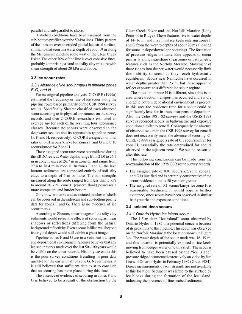
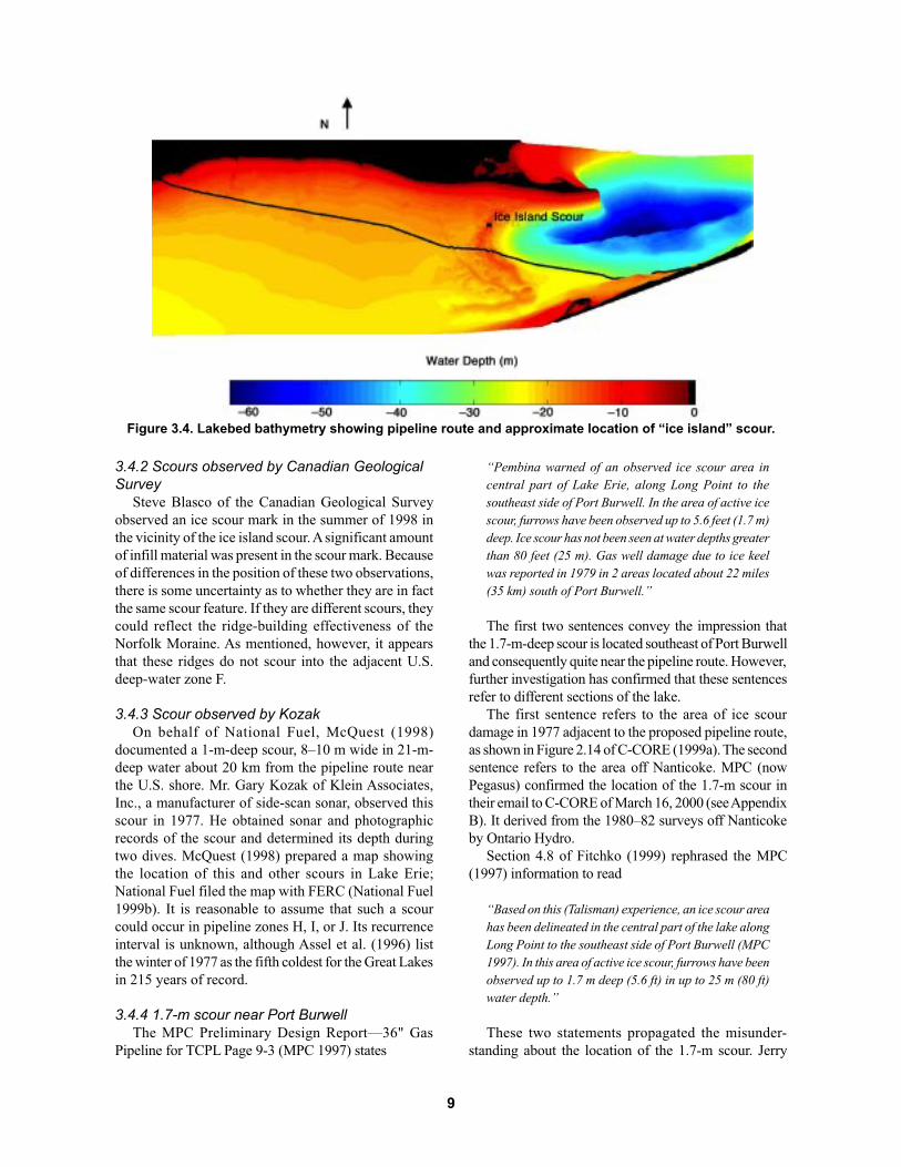
definitions ........................................................................................................ 43.3. Survey routes for U.S. Geological Survey cruises 1991–1993 ........................ 73.4. Lakebed bathymetry showing pipeline route and approximate location

of “ice island” scour ........................................................................................ 94.1 Millennium pipeline route, Talisman gas pipelines on the seabed, and

recorded dates of pipeline damage .................................................................. 105.1. Depth distribution of “new” scours compiled from 1995 Ohio

Geological Survey data .................................................................................... 135.2 Depth distribution of “new” scours compiled from Ontario Hydro 1981

and 1982 surveys (Coho) and from Canadian Seabed Research 1998route survey ..................................................................................................... 14

5.3. Depth distribution of “new” scours compiled from the Ontario Hydro1981 and 1982 surveys (Coho), from the Ohio 1995 survey, and fromthe Canadian Seabed Research 1998 route survey .......................................... 14

5.4. Exponential fit to depth distribution of “new” scours compiled fromOntario Hydro 1981 and 1982 surveys (Coho), from Ohio GeologicalSurvey 1995 survey, and from Canadian Seabed Research 1998route survey ..................................................................................................... 16

6.1. Schematic of finite-element model and geometric boundary condition ........... 206.2. Plan view of the horizontal profile sub-scour soil displacement ...................... 206.3. Progression of scouring ice keel–trench interaction ......................................... 216.4. Transverse horizontal load-displacement relationship for Case X ................... 236.5. Transverse horizontal soil reaction load for Case X ......................................... 246.6. Profile of the imposed subgouge displacement field and computed

pipeline displacement response for Case X ..................................................... 246.7. Longitudinal distribution of axial strain for Case X ......................................... 25

TABLES

Table3.1. Original and revised Millennium pipeline zones in U.S. waters ...................... 43.2. Expanded ice scour data set relevant to Millennium pipeline route ................. 53.3. Summary of “new” scour depth data for Lake Erie ......................................... 63.4. Scour depth distribution from 1995 Ohio Geological Survey data .................. 74.1. Water depth distribution ................................................................................... 115.1. Millennium pipeline zones in U.S. waters defined in C-CORE ....................... 165.2. Revised 10-year and 100-year scour depths for Millennium pipeline

zones in U.S. waters ........................................................................................ 176.1. Summary of recommendations revised ............................................................ 226.2. Models supporting trench depth recommendations .......................................... 238.1. Sources and sinks of metals in Lake Erie ......................................................... 318.2. Correlation of metals, PCBs, and organic carbon in Lake Erie sediments ....... 328.3. Correlation of metals and organic carbon in composite sediment core

samples collected along the Millennium Lake Erie Crossing route ................ 338.4. Mean concentrations of metals in precolonial sediments and in the

composite sediment cores collected along the proposed pipeline route .......... 338.5. Sedimentation rates in eastern basin of Lake Erie ............................................ 348.6. Surficial sediment core sample logs ................................................................. 35(9.) 1. Deposition for unidirectional spreading ....................................................... 45(9.) 2. Deposition for bi-directional spreading ........................................................ 45

10.1. Revised 100-year scour depths and design trench depths for Millenniumpipeline zones in U.S. waters .......................................................................... 46

v

EXECUTIVE SUMMARY

The Millennium Pipeline Project includes a crossing of Lake Erie to bring Canadiannatural gas to markets in the eastern United States. Millennium proposes to lay this 1.07-m-diameter, concrete-coated pipeline in a trench excavated in the lakebed to protect it fromscouring ice keels, fishing gear, and anchors.

In response to a request from the Federal Energy Regulatory Commission, researchers atERDC assessed Millennium’s work on three topics related to the Lake Erie crossing:

• The potential for pipeline damage by ice scour.• The adequacy of the sampling program to identify contaminated sediments.• The adequacy of the modeling for turbidity and sediment deposition resulting from trench

excavation.

This assessment focused on the pipeline zones in U.S. waters and was conducted incollaboration with Millennium, its partners, and the Pittsburgh District, Corps of Engineers.

High winds on Lake Erie can fracture and pile ice into large ridges. Ice scour occurswhen the keels of these ridges drag along the lakebed. To avoid damage, a pipeline must bedesigned to withstand the forces from an ice scour expected to cross the pipeline, on average,once in 100 years. The design trench depth must place the pipe crown sufficiently below thescour depth to keep pipe deformations within acceptable limits.

Determination of the 100-year ice scour depth was the only issue that required additionalanalyses to satisfy the concerns of the ERDC reviewers. The original analyses relied solelyon data from a single survey along the pipeline route. The ERDC review resulted in twomain changes: only new scours were used to determine the scour-depth probabilitydistribution, and scour data from comprehensive surveys nearby the pipeline route wereincluded. These changes increased the estimated 100-year scour depth by 25%, from 1.2 to1.5 m, in pipeline zones nearest to the U.S. shore (zones H, I, and J). In these zones thedesign trench depth increased by about 20%, from 2.8 to 3.4 m (Table E1). Ice scour doesnot control trench depths in deep-water zones F and G, and the originally designed trenchdepth of 2.0 m is adequate even if it did. Additional benchmark analyses conducted duringthe ERDC review increase confidence in the estimated scour rates, the scour-depthdistribution, and the resulting 100-year scour depths.

The ERDC assessment included the pipe–soil interaction model used to determine thedesign trench depths given the 100-year scour depth for each zone. This finite-elementmodel relies on results from centrifuge tests and field observations, and it represents thestate of the art. A question–answer exchange resolved concerns regarding use of two-dimensional modeling, the choice of soil-stiffness characteristics, and the response of thepipe in a partially backfilled trench. Conservative choices regarding normal incidence angleand keel–pipe load transfer through native soil increase confidence in the model results.

ERDC’s assessment of Millennium’s sediment-sampling program sought to resolve issuesconcerning the depth and intensity of sampling and the use of mercury as an indicatorcontaminant. A question–answer exchange, which included additional data and references,resolved these concerns. No additional sampling or analyses are needed due to increasedtrench depths because the extra material excavated would be uncontaminated.

ERDC’s assessment of Millennium’s modeling of turbidity and sediment depositionfocused on the modeling methods and the choice of sediment settling velocity. Many specific

vi

issues were resolved through a question–answer exchange. Modeling by ERDC showedthat the originally predicted turbidity plume is conservative. However, Millennium willneed to update its results to show as much as a factor-of-three short-term increase in theexpected thickness of the sediment blanket adjacent to the pipeline trench. A 20% increasein design trench depths would result in a further 10% increase in blanket thickness and a10% increase in blanket width. The effect on the turbidity plume would depend on thetrench excavation rate. Millennium agreed with the results of this review.

The design of the pipeline includes a margin of safety between the maximum tensilestrain caused by the 100-year scour (2.5%) and strain needed to rupture the pipe (about3.8%). Millennium will monitor the pipeline continuously for changes in conditions thatcould signal damage and would close valves at each side of the lake if a leak occurs. Inaddition, Millennium will conduct internal and external inspections of the pipeline atapproximately three-year intervals (depending on ice conditions) to detect possible damageand to assess the design for ice scour protection. It will also establish procedures (as requiredby regulation) for emergency response and repair of the pipeline.

In conclusion, the ERDC assessment of Millennium Pipeline Project’s Lake Erie crossingrevealed the need for two revisions: a 20% increase in design trench depths in zones H, I,and J, and as much as a threefold short-term increase in expected sediment-blanket thicknessadjacent to the excavated trench. Otherwise, the analyses conducted and reports preparedby Millennium pertaining to the three topics assessed are technically sound and satisfy therequest for additional information under the Corps of Engineers regulatory review process.

Table E1. Revised 100-year scour depths and design trench depths for Millen-nium pipeline zones in U.S. waters. Original scour and trench depths are from C-CORE (1999a), although zone definitions differ slightly.

Original Revised Original Revised

Distance from Start–end 100-year 100-year design design

Canadian water depth scour scour trench trench

Pipeline landfall range depth depth depth depth

zone (km) (m) (m) (m) (m) (m)

F 98.0–105.0 21.0–26.7 0.8* 0.8* 2.0 2.0

G 105.0–135.1 26.7–27.4 0.8* 0.8* 2.0 2.0

H 135.1–136.8 27.4–18.4 1.2 1.5 2.8 3.4

I 136.8–142.2 18.4–16.4 1.2 1.5 2.8 3.4

J 142.2–147.3 16.4–17.1 1.2 1.5 2.8 3.4

ALF 147.3–149.3 (DDA) 17.1–8.3

ALF: American Landfall

DDA: End of Directionally Drilled Pipe from American Landfall

* Assigned values based on need to protect pipeline from anchors and fishing gear. Ice scour does

not control trench depths for zones F and G.

vii

viii

PARTICIPANTS

ERDC Review Team

Dr. James M. Brannon Dr. Mark S. DortchEnvironmental Laboratory Environmental LaboratoryWaterways Experiment Station Waterways Experiment StationVicksburg, Mississippi 39180-6199 Vicksburg, MS 39180-6199

Mr. Scott A. Hans Dr. Steven A. KetchamU.S. Army Engineer District, Pittsburgh Cold Regions Research andPittsburgh, Pennsylvania 15222-4186 Engineering Laboratory

Hanover, New Hampshire 03755-1290

Dr. James H. Lever, Team Leader Dr. Paul R. SchroederCold Regions Research and Environmental Laboratory

Engineering Laboratory Waterways Experiment StationHanover, New Hampshire 03755-1290 Vicksburg, Mississippi 39180-6199

Millennium Participants

Mr. James R. Albitz Dr. Jerry FitchkoColumbia Gas Transmission BEAK International, Inc.Binghamton, New York 13902 Brampton, Ontario L6T 5B7

Mr. Richard E. Hall, Jr., Coordinator Dr. Richard F. McKennaColumbia Gas Transmission C-COREBinghamton, New York 13902 Memorial University of NewfoundlandC-CORE St. John’s, Newfoundland A1B 3X5

Mr. Peter Patient Dr. Ryan PhillipsTransCanada Transmission C-CORECalgary, Alberta T2P 3P7 Memorial University of Newfoundland

St. John’s, Newfoundland A1B 3X5

Mr. James M. Shearer Mr. Gerard J. Van ArkelShearer Consulting BEAK International, Inc.Ottawa, Ontario K1S 2S8 Brampton, Ontario L6T 5B7

Assessment of Millennium Pipeline ProjectLake Erie Crossing

Ice Scour, Sediment Sampling, and Turbidity Modeling

JAMES H. LEVER, EDITOR

1.0 INTRODUCTION

Millennium Pipeline Company (Millennium)proposes to construct and operate a pipeline to transportCanadian natural gas to markets in the eastern UnitedStates. The project includes a crossing of Lake Erie,from Patrick Point, Ontario, to a location close to theTown of Ripley, New York, a length of about 150 km.The pipeline would consist of 0.91-m-diameter steelpipe, with a 7.5-cm concrete coating for stability.Millennium proposes to lay this pipeline in a trenchexcavated in the lakebed to protect it from scouring icekeels, fishing gear, and anchors.

The Federal Energy Regulatory Commission(FERC) received numerous public comments inresponse to its Draft Environmental Impact Statementon the Millennium project (FERC 1999). FERCrequested technical assistance from the U.S. ArmyCorps of Engineers (USACE) to address comments onthree topics related to the Lake Erie crossing:

• The potential for pipeline damage by ice scour.• The adequacy of the sampling program to identify

contaminated sediments.• The adequacy of the modeling for turbidity and

sediment deposition and resulting from trenchexcavation.

The U.S. Army Engineer Research and DevelopmentCenter (ERDC), in collaboration with Millennium, itspartners, and the Pittsburgh District, Corps of Engineers,assessed Millennium’s work on these three topics.ERDC researchers at the Cold Regions Research andEngineering Laboratory (CRREL) assessed the designfor ice scour, while researchers at the Environmental

Laboratory (EL) assessed the sediment samplingprogram and turbidity modeling.

Each ERDC group reviewed Millennium projectmaterials, public comments, and the open literaturerelated to its topic. As needed, these groups requestedclarification or additional analyses by Millennium onspecific issues and conducted their own independentanalyses. This report describes the findings of the ERDCteam and the recommended changes in Millenniumproject specifications needed to address FERC andUSACE permit requirements. Appendix A lists the mainproject and public-comment documents reviewed.

2.0 SCOPE AND TECHNICAL ISSUES

2.1 U.S. side focusApproximately 98 km of the Millennium pipeline

crossing of Lake Erie are in Canadian waters. Theremaining 51 km are in U.S. waters and consequentlyare subject to the regulatory jurisdiction of FERC andUSACE. Although geophysical and environmentalinformation from the entire lake was used in ERDCreviews and analyses, the resulting assessments andrecommendations are limited to the portion of theproject in U.S. waters.

2.2 Ice scour issuesThe process of ice scour on Lake Erie is similar to

that occurring in the near-shore zones of the U.S. andCanadian Beaufort Seas and other coastal arctic areas(see, for example, Lewis 1977, Weeks et al. 1983, Grass1984, Niedoroda 1991). On Lake Erie, strong windscan cause ice to fracture and pile up into ridges reaching

2

10 m high. Subsequent movement of these ridges cancause their keels to drag along the lakebed, producingnear-linear furrows or scours. Scours up to 1.5 m deep,100 m wide, and several kilometers long, in water depthsup to 27.4 m, have been observed. Ice scouring in LakeErie is episodic, with high spatial and temporalvariability of scour formation and infilling by sediments.

No operational marine pipelines exist that weredesigned to resist damage by scouring ice keels.Nevertheless, a consensus exists regarding designprocedures (Weeks et al. 1983, Niedoroda 1991,Woodworth-Lynas et al. 1996). The Northstar oilpipeline in the Beaufort Sea near Prudhoe Bay, Alaska,was so designed (INTEC 1998a, 1998b), receivedUSACE permits, and was recently constructed. Codesfor marine pipelines recognize the random nature ofenvironmental loads and require designing for suchloads with an expected annual risk of 0.01, equivalentto a return period of 100 years (ASME 1995, CSA1999). For loads due to scouring ice keels, the designprocess basically is as follows:

• Predict the 100-year ice scour depth along theproposed route.

• Predict the soil deformation resulting from that scour.• Select a combination of trench depth and pipe design

to ensure that pipe deformation in response to thisevent is within acceptable levels.

C-CORE, long involved with the study of ice scourprocesses, conducted these analyses on behalf ofMillennium for the Lake Erie crossing (C-CORE1999a). Their design process was similar to the one usedfor the Northstar project (C-CORE 1999b).Nevertheless, detailed technical objections were raisedduring the FERC and USACE public comment periods,primarily by National Fuel Gas Supply Corporation(National Fuel 1999a, 1999b, 2000).

ERDC researchers examined the Millennium projectmaterials, C-CORE’s design for ice scour protection,and the technical objections raised. Summarized beloware the main issues we sought to resolve during thisreview.

2.2.1 Prediction of 100-year ice scour depthTwo sets of information are required to predict the

100-year scour depth along a proposed route: thedistribution of scour depths and the rate that scoursoccur. Repetitive geophysical mapping of the proposedroute is the preferred method to obtain this information.However, it can take many years to build a sufficientlylarge database of scours for locations such as Lake Erie,where scour rates are low (< 1 scour/km/yr). Otherenvironmental data and knowledge of ice scour

processes can be used to supplement route-specific data.C-CORE’s original design for ice scour protection

(C-CORE 1999a) relied primarily on data from a singlegeophysical survey along the Millennium route,conducted by Canadian Seabed Research (CSR) in1998. They compiled a distribution of scour depthsusing both newly formed and infilled scours. Theyestimated scour rates by classifying each scouraccording to its qualitative appearance and thenestimating the average age for each class. This relianceon a single survey raised several concerns:

• Only six measured scours were newly formed, andno allowance was made for sediment infilling of olderscours.

• Episodic scour formation and infill processes in LakeErie suggest a need for a longer sample interval.

• Individual scours much deeper than those measuredby the 1998 survey have been observed near theproposed route.

• Qualitative age classes introduce large uncertaintiesin the calculated scour rates.

• The small total number of measured scour depthsintroduces uncertainty in the estimated depthdistribution.

• Lack of in-service experience with pipelines exposedto ice scour suggests a need for conservatism in theanalyses.

C-CORE countered that the depth distribution ofexisting scours can approximate that for new scours(Lewis 1977, Lanan et al. 1986), that it is difficult toassign recurrence rates to individual deep scours, thatthey calibrated their scour-rate method using othersurveys from Lake Erie, and that compoundingconservatism can make the effective design returninterval much longer than the 100-year coderequirement. Nevertheless, we agreed that additionalanalysis of ice scour data from Lake Erie, selectedsensitivity analyses, allowance for conservatism in thedesign method, and comparisons with benchmarkcalculations could increase confidence in the predicted100-year scour depth.

C-CORE and members of the ERDC review teamconducted this additional work collaboratively. Chapters3–5 describe this work and the recommended changesto the 100-year scour depths used to design the pipeline.

2.2.2 Prediction of soil deformation and pipelineresponse

Researchers at C-CORE were the first to discoverthat significant soil movement occurred beneathscouring ice keels and that this movement could deliverlarge loads on marine pipelines buried below the scour

3

depth (Woodworth-Lynas et al. 1996). They led a joint-industry research project termed PRISE (Pressure RidgeIce Scour Experiment) to quantify this effect. PRISEconsists of centrifuge modeling, finite-element analyses,and field studies. Its results are proprietary to theparticipants, although relevant results were madeavailable to the ERDC review team (C-CORE 1998).

The issues raised during public comment and theERDC review focused primarily on the assumptionsmade to model the soil–pipeline interaction. Theseincluded use of two-dimensional (rather than three-dimensional) modeling, ignoring the presence of apartially filled trench, and details regarding the choiceof soil-stiffness parameters. C-CORE addressed theseissues through a question–answer process, and noadditional analyses were needed. Chapter 6 describesthe soil–pipeline interaction modeling and the ERDCreview of it.

2.3 Sediment sampling and deposition/turbidity modeling

Millennium proposes to excavate the pipeline trenchusing mechanical jetting and suctioning and lateraldisplacement of the excavated sediments (FERC 1999).BEAK International, Inc. (BII), on behalf ofMillennium, conducted sediment sampling along theproposed route and analyses of the samples forcontamination. They also modeled the deposition of thedisplaced sediments and the extent and concentration

of the turbidity plume. Technical concerns over detailsof this work were raised during public comment.

Lake Erie sediments are known to contain heavymetal and organic contaminants. Concerns about theadequacy of the sampling program included locationsof samples, depths of sampling, and the use of mercuryas an indicator contaminant. Concerns about sedimentdeposition and the turbidity plume focused on specificsof the modeling method used to predict these effectsand consequently on the accuracy of the predictions.Researchers at the ERDC Environmental Laboratory(EL) assessed these concerns, sought clarification, andassessed Millennium’s answers. In most cases, noadditional analyses were required. Chapters 8 and 9summarize their findings.

3.0 SUMMARY OF ICE SCOUR DATA

3.1 Zone definitions and focus of data reviewC-CORE (1999a) divided the Millennium pipeline

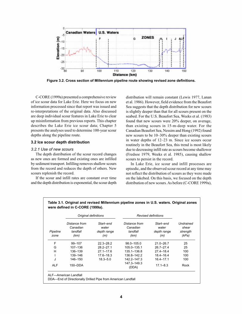
Lake Erie crossing into zones A through J based onwater depth, soil type, and exposure to scouring icefeatures. The pipeline routing was changed slightly inlate 1998, which necessitated a change in the zonedefinitions. Figures 3.1 and 3.2 show the revised zones,and Table 3.1 provides the water depth ranges andextents of each zone. Note that the beginning of zone Fcoincides with the U.S.–Canada international boundary.

Figure 3.1. Millennium pipeline zones in U.S. waters.

4

C-CORE (1999a) presented a comprehensive reviewof ice scour data for Lake Erie. Here we focus on newinformation processed since that report was issued andre-interpretations of the original data. Also discussedare deep individual scour features in Lake Erie to clearup misinformation from previous reports. This chapterdescribes the Lake Erie ice scour data; Chapter 5presents the analyses used to determine 100-year scourdepths along the pipeline route.

3.2 Ice scour depth distribution

3.2.1 Use of new scoursThe depth distribution of the scour record changes

as new ones are formed and existing ones are infilledby sediment transport. Infilling removes shallow scoursfrom the record and reduces the depth of others. Newscours replenish the record.

If the scour and infill rates are constant over timeand the depth distribution is exponential, the scour depth

distribution will remain constant (Lewis 1977, Lananet al. 1986). However, field evidence from the BeaufortSea suggests that the depth distribution for new scoursis slightly deeper than that for all scours present on theseabed. For the U.S. Beaufort Sea, Weeks et al. (1983)found that new scours were 20% deeper, on average,than existing scours in 15-m-deep water. For theCanadian Beaufort Sea, Nessim and Hong (1992) foundnew scours to be 10–30% deeper than existing scoursin water depths of 12–23 m. Since ice scours occurroutinely in the Beaufort Sea, this trend is most likelydue to decreasing infill rate as scours become shallower(Fredsoe 1979, Weeks et al. 1985), causing shallowscours to persist in the record.

In Lake Erie, ice scour and infill processes areepisodic, and the observed scour record at any time maynot reflect the distribution of scours as they were madeon the lakebed. On this basis, we focused on the depthdistribution of new scours. As before (C-CORE 1999a),

Figure 3.2. Cross section of Millennium pipeline route showing revised zone definitions.

Table 3.1. Original and revised Millennium pipeline zones in U.S. waters. Original zoneswere defined in C-CORE (1999a).

Original definitions Revised definitions

Distance from Start–end Distance from Start–end UndrainedCanadian water Canadian water shear

Pipeline landfall depth range landfall depth range strengthzone (km) (m) (km) (m) (kPa)

F 99–107 22.3–28.2 98.0–105.0 21.0–26.7 25G 107–136 28.2–27.1 105.0–135.1 26.7–27.4 25H 136–139 27.1–17.6 135.1–136.8 27.4–18.4 100I 139–146 17.6–18.3 136.8–142.2 18.4–16.4 100J 146–150 18.3–5.0 142.2–147.3 16.4–17.1 100

147.3–149.3ALF 150–DDA

(DDA)17.1–8.3 Rock

ALF—American LandfallDDA—End of Directionally Drilled Pipe from American Landfall

5

new scours are defined as those for which all details ofthe original scour mounds and scour base are visibleon the survey records. They exhibit little or no evidenceof infilling. Consequently the measured depthapproximates the depth of the original incision.

3.2.2 Sampling the scour depth distributionWe have also concentrated on populations of scours

from comprehensive lakebed surveys, ones conductedusing sidescan sonar and a sub-bottom profiler todocument scour width, depth, and appearance. Typicallycomprehensive surveys consist of a series of linearsurveys along individual scours, along the routeproposed for a pipeline or cable crossing, or within anarea to construct a mosaic. The data from such surveysare, insofar as possible, unbiased with respect to soil,ice, and bathymetric conditions that govern the ice scourprocess.

Isolated scours found on an opportunity basis shouldbe considered carefully since they represent biasedsamples. For example, a few individual scours withdepths greater than about 1 m have been measured inLake Erie. While these are useful for comparison withpredicted extreme values, in general they should not belumped with data from comprehensive surveys. It isdifficult to establish the frequency of occurrence ofindividual deep scours, and many shallow scours shouldaccompany each deep one if they derive from the samepopulation.

For frequent processes such as winds and waves, itis sufficient to consider only the largest events forengineering design. Often only annual maxima are usedto predict 100-year events. However, the ice scourprocess is generally less frequent, and historical recordsare shorter. Consequently even in the Beaufort Sea allscours in a region have been used to characterize thedepth distribution for design purposes (INTEC 1998a,

1998b). This approach is particularly appropriate forLake Erie, where scour rates are lower and no long-term studies exist.

Twenty-five scour marks with measurable depthwere identified in the 1998 CSR route survey. Sinceonly a handful of these can be considered “new” scours,we examined data from other lakebed surveysconducted by a variety of agencies for differentpurposes. The context of these surveys, and of individualdeep scours found outside of comprehensive surveys,bear on their use in predicting the 100-year ice scourdepth. The relevant data sources for analysis of designscour depth along the proposed Millennium pipelineroute are listed in Table 3.2. Details of these data arefound in Sections 3.2.3, 3.2.4, and 3.2.5.

3.2.3 Millennium route surveysScour depth from 1997 route survey. All of the ice

scours surveyed by Racal in 1997 were resurveyed byCanadian Seabed Research in 1998 (C-CORE 1999a).Since the latter survey yielded higher-quality data andno new scours, we have not used the 1997 data.

Scour depth from 1998 route survey. The 1998 CSRsurvey documents scour depths along the pipelineroute, in the U.S. and Canadian landfall areas, and alongthe Clear Creek Esker (C-CORE 1999a). Data fromthis survey were reinterpreted, and only scours classi-fied as new were retained. For scours that were sur-veyed several times along their tracks, we included inthe database only the greatest measured depth for eachscour.

Two scours were observed as having significant andmeasurable infilling. These were assumed to haveoriginal depths equal to the measured depth plus theinfilled amount. These two scours were thereforereclassified as “new.” Table 3.3 lists the scour depth

Table 3.2. Expanded ice scour data set relevant to Millennium pipeline route.

Source Year Location Details

Ontario Hydro 1981 Coho (U.S. shore) Interpreted by Ontario Hydro(C-CORE 1999a, Table 2.5)

Ontario Hydro 1982 Coho (U.S. shore) Interpreted by Ontario Hydro(C-CORE 1999a, Table 2.5)

Ohio 1995 U.S. shore Interpreted by Jim Shearer(this document, Table 3.4)

CSR 1998 Pipeline Route Interpreted by Jim Shearer(C-CORE 1999a, Appendix D)

6

and the water depth of the resulting eight new scoursfrom the 1998 CSR survey.

3.2.4 Ontario Hydro surveysOntario Hydro conducted a series of linear and area

surveys in the early 1980s to support the design of aproposed submarine transmission cable (Grass 1984).Most of the work focused on the U.S. and Canadiannear-shore zones (Coho and Nanticoke regions,respectively).

Coho region. We included in our analyses data fromOntario Hydro surveys near Coho on the U.S. shore.This region is reasonably close to the pipeline route,and it has similar soil, bathymetric, and ice-exposureconditions to zones H, I, and J of the pipeline route.

Eight ice scours ranging from 0.1 to 0.5 m were iden-tified in the Coho area (Table 3.3). These represent allscours with measurable depth identified by OntarioHydro in this area during 1981 and 1982 surveys (C-CORE 1999a). The original sidescan data have not beenreanalyzed. Grass (1984) described how the scoursobserved each year were not present the previous year.Thus, we classified all eight as new scours.

Nanticoke region. Ontario Hydro data from theNanticoke region have been excluded from our designanalysis. The scours occurred in much softer soil thanfound along the Millennium pipeline route, and theyappear to represent a different population from thescours recorded by the other Lake Erie surveys.

Many of the ice scours surveyed by Ontario Hydroat Nanticoke were found in cohesive soils withundrained shear strengths of less than 12.5 kPa. Scoursalong the pipeline route have been observed only insand and in cohesive soils with shear strengths in excessof 50 kPa. Insufficient data exist to transform the scourdepths from Nanticoke to the stronger soils along theproposed Millennium route.

Fourteen Nanticoke scours were identified in sand/gravel deposits. In principle, these scours could beincluded in the design analysis for the Millennium route.However, shear strengths of 25 kPa were associatedwith two of the fourteen scours. This strength isinconsistent with sand and gravel deposits, and moredetailed geotechnical data are not available. Also, thesix Nanticoke scours in sand/gravel with measurabledepths occur in water deeper than 23 m, and theiraverage scour depth is 0.61 m. This is much deeperthan the average depths of the other Lake Erie data sets,and indeed it is deeper than would be expected in theU.S. Beaufort Sea for similar water depths (Weeks etal. 1983). The occurrence of such deep scours in deepwater suggests an exposure to ice scour conditions verydifferent from those along the Millennium route. Forthese reasons, we have not included any of theNanticoke scours in the pipeline design analyses.

3.2.5 Other surveys in U.S. watersOverview. C-CORE (1999a) summarized the known

lakebed surveys conducted in U.S. waters. Of these themost relevant were conducted by the U.S. Geological

Table 3.3. Summary of “new” scour depth data for Lake Erie.

Source Water depth (m) Scour depth (m)

17 0.212.4 0.4

Ontario Hydro 1981 24.7 0.2Coho Area Survey 21.9 0.2

13.8 0.217.2 0.4

Ontario Hydro 1982 21.9 0.1Coho Area Survey 23.7 0.5

Ohio Geological Survey 1995 14–16 See Table 3.4

18.3 0.520.25 0.719.5 0.6

Canadian Seabed Research 1998 8.6 0.3Pipeline Route Survey 8.4 0.2

8.4 0.29.8 0.19.8 0.5

Survey in 1992 and 1993 and by the Ohio GeologicalSurvey in 1995. These surveys are the most easterlyones illustrated in Figure 3.3 and included sidescansonar and sub-bottom profiler data.

Mr. Jim Shearer, a consultant with extensiveexperience analyzing ice scour surveys, examined theoriginal records from these three surveys. He identified50 km of survey lines from 1995 that overlapped withlines from 1992 and identified numerous new scoursby comparing the two records. Their similar freshappearance suggested that these scours all derived fromthe winter or early spring of 1994, when severe iceconditions and strong winds were reported (Assel et al.1996).

Scour marks were also identified in the 1992 and1993 surveys. However, these showed signs of

significant infilling and have not been included in thepipeline design analyses.

Ohio Geological Survey 1995. A detailed examina-tion was undertaken of the sonar survey conducted bythe Ohio Geological Survey division in 1995. The 50km that overlapped with 1992 consisted of two surveylines parallel to the U.S. shore. These lines, in waterdepths of 14–16 m, run from the Ohio–Pennsylvaniaborder to a point about 50 km to the southwest.

In total, Shearer identified 96 new scours. Abreakdown of their depth distribution is listed in Table3.4. The greatest scour depth measured was 0.6 m.Although the two survey lines were only 1 km apart, itis not believed that more than 10% are scours commonto both lines because the observed scours were primarily

Figure 3.3. Survey routes for U.S. Geological Survey cruises 1991–1993.

Table 3.4. Scour depth distribution from 1995 Ohio Geo-logical Survey data.

Number of scours

Scour depth range (m) Line

Minimum Maximum L-29 L-28 Total

0.00 0.10 15 15 300.10 0.15 11 12 230.15 0.25 14 8 220.25 0.35 9 1 100.35 0.45 6 1 70.45 0.55 3 30.55 0.65 1 1

Total 58 38 96

7

parallel and sub-parallel to shore. Lakebed conditions have been assessed from the

sub-bottom profiler over the 50-km lines. Thirty percentof the lines are over an eroded glacial lacustrial surface,similar to that seen in a water depth of about 19 m alongthe Millennium pipeline route west of the Clear CreekEsker. The other 70% of the line is over cohesive fines,probably comprising a sand and silty clay mixture withshear strength of about 20 kPa and above.

3.3 Ice scour rates

3.3.1 Absence of ice scour marks in pipeline zonesF, G, and H

For its original pipeline analysis, C-CORE (1999a)estimated the frequency or rate of ice scour along thepipeline route based primarily on the CSR 1998 surveyresults. Specifically Shearer classified each observedscour according to its physical appearance on the surveyrecords, and then C-CORE researchers estimated anaverage age for each of the resulting four appearanceclasses. Because no scours were observed in thedeepwater section and its approaches (pipeline zonesG, F, and H, respectively), C-CORE assigned nominalrates of 0.01 scours/km/yr for Zones F and G and 0.10scours/km/yr for Zone H.

These assigned scour rates were reconsidered duringthe ERDC review. Water depths range from 21.0 to 26.7m in zone F, exceed 26.7 m in zone G, and range from27.4 to 18.4 m in zone H. In zones F and G, the lakebottom sediments are composed entirely of soft siltyclays to a depth of 5 m or more. The soil strengthsmeasured along the route ranged from less than 5 kPato around 50 kPa. Zone H (eastern flank) possesses amore competent and harder bottom.

Only trawler marks and associated patches of shellscan be observed in the sidescan and sub-bottom profiledata for zones F and G. There is no evidence of icescour marks.

According to Shearer, sonar images of the silty claysediments would reveal the effects of scouring as linearshadows or reflections differing from the naturalbackground reflectivity. Even a scour infilled well beyondits original depth would still exhibit a ghost image.

Pipeline zones F and G are in a sediment transportand depositional environment. Shearer believes that anyice scour marks made over the last 50–100 years wouldbe visible on the sonar records. His only caveat to thisis the poor survey conditions (resulting in poor dataquality) for the eastern half of zone G. Nevertheless, itis still believed that sufficient data exist to concludethat no scouring has taken place during this time.

The absence of evidence of scouring in zones F andG is believed to be a result of the obstruction by the

Clear Creek Esker and the Norfolk Moraine (LongPoint–Erie Ridge). These features rise to water depthsof 14–16 m, and may limit ice keels entering zones Fand G from the west to depths of about 20 m (allowingfor some upslope/downslope scouring). The formationof pressure ridges on Lake Erie appears to occurprimarily along near-shore shear zones or bathymetricfeatures such as the Norfolk Moraine. Movement ofthese ridges into deeper water would necessarily limittheir ability to scour as they reach hydrostaticequilibrium. Scours near Nanticoke have occurred inwater depths greater than 23 m, but these appear toreflect exposure to a different ice scour regime.

The situation in zone H is different, since this is anarea where traction transport has occurred and a moreenergetic bottom depositional environment is present.In this area the residence time for a scour could besignificantly less than in areas of suspension deposition.Also, the Coho 1981–82 surveys and the USGS 1993surveys recorded scours in bathymetric and exposureconditions similar to zone H. Consequently the absenceof observed scours in the CSR 1998 survey for zone Hdoes not necessarily mean the absence of scouring. C-CORE (1999a) assigned a rate of 0.1 scours/km/yr forzone H, essentially the rate determined for scoursobserved in the adjacent zone I. We see no reason toalter this rate.

The following conclusions can be made from there-examination of the 1998 CSR route survey records:

• The assigned rate of 0.01 scours/km/yr in zones Fand G is justified and is certainly conservative if thescour residence time is 50 years or greater.

• The assigned rate of 0.1 scours/km/yr for zone H isreasonable. Reducing it would require furtherevidence, since scours have been observed in similarbathymetric and exposure conditions.

3.4 Isolated deep scours

3.4.1 Ontario Hydro ice island scourThe 1.5-m-deep “ice island” scour observed by

Ontario Hydro in 1982 is a potential concern becauseof its proximity to the pipeline. This scour was observedon the Norfolk Moraine at the location shown in Figure3.4. The water depth of the scour mark was 16–19 m,and this location is potentially exposed to ice keelsmoving from deeper water onto this shelf. The scour isbelieved to have been caused by the “ice island”pressure ridge documented extensively on video by JimGrass of Ontario Hydro in February 1982 (Grass 1984).Direct measurements of soil strength are not availableat this location. Sediment was lifted to the surface byice blocks during the formation of the ice island,indicating the presence of fine seabed sediments.

8

3.4.2 Scours observed by Canadian GeologicalSurvey

Steve Blasco of the Canadian Geological Surveyobserved an ice scour mark in the summer of 1998 inthe vicinity of the ice island scour. A significant amountof infill material was present in the scour mark. Becauseof differences in the position of these two observations,there is some uncertainty as to whether they are in factthe same scour feature. If they are different scours, theycould reflect the ridge-building effectiveness of theNorfolk Moraine. As mentioned, however, it appearsthat these ridges do not scour into the adjacent U.S.deep-water zone F.

3.4.3 Scour observed by KozakOn behalf of National Fuel, McQuest (1998)

documented a 1-m-deep scour, 8–10 m wide in 21-m-deep water about 20 km from the pipeline route nearthe U.S. shore. Mr. Gary Kozak of Klein Associates,Inc., a manufacturer of side-scan sonar, observed thisscour in 1977. He obtained sonar and photographicrecords of the scour and determined its depth duringtwo dives. McQuest (1998) prepared a map showingthe location of this and other scours in Lake Erie;National Fuel filed the map with FERC (National Fuel1999b). It is reasonable to assume that such a scourcould occur in pipeline zones H, I, or J. Its recurrenceinterval is unknown, although Assel et al. (1996) listthe winter of 1977 as the fifth coldest for the Great Lakesin 215 years of record.

3.4.4 1.7-m scour near Port BurwellThe MPC Preliminary Design Report—36" Gas

Pipeline for TCPL Page 9-3 (MPC 1997) states

“Pembina warned of an observed ice scour area incentral part of Lake Erie, along Long Point to thesoutheast side of Port Burwell. In the area of active icescour, furrows have been observed up to 5.6 feet (1.7 m)deep. Ice scour has not been seen at water depths greaterthan 80 feet (25 m). Gas well damage due to ice keelwas reported in 1979 in 2 areas located about 22 miles(35 km) south of Port Burwell.”

The first two sentences convey the impression thatthe 1.7-m-deep scour is located southeast of Port Burwelland consequently quite near the pipeline route. However,further investigation has confirmed that these sentencesrefer to different sections of the lake.

The first sentence refers to the area of ice scourdamage in 1977 adjacent to the proposed pipeline route,as shown in Figure 2.14 of C-CORE (1999a). The secondsentence refers to the area off Nanticoke. MPC (nowPegasus) confirmed the location of the 1.7-m scour intheir email to C-CORE of March 16, 2000 (see AppendixB). It derived from the 1980–82 surveys off Nanticokeby Ontario Hydro.

Section 4.8 of Fitchko (1999) rephrased the MPC(1997) information to read

“Based on this (Talisman) experience, an ice scour areahas been delineated in the central part of the lake alongLong Point to the southeast side of Port Burwell (MPC1997). In this area of active ice scour, furrows have beenobserved up to 1.7 m deep (5.6 ft) in up to 25 m (80 ft)water depth.”

These two statements propagated the misunder-standing about the location of the 1.7-m scour. Jerry

Figure 3.4. Lakebed bathymetry showing pipeline route and approximate location of “ice island” scour.

9

Fitchko of BEAK verbally confirmed to C-CORE thatthe 1.7-m scour relates to the area off Nanticoke.

The Pembina gas pipeline system in Lake Erie wasacquired recently by Talisman Energy. Appendix C is aletter from Talisman Energy to TransCanadaTransmission dated 22 September 1999. This lettercovered the chart of known locations of damage to theTalisman system. The letter states that

“All visible scouring we have experienced has beenlimited to a maximum depth of 2 feet into the lakebottom....”

This statement confirms that Pembina did not observea 1.7-m-deep scour within its system, including areasclose to the Millennium pipeline route.

3.4.5 Purported 3.6-m-deep scourIn Ontario Hydro internal report 80463, Mr. Jim

Grass referenced a possible 3.6-m-deep scour southeastof Port Burwell (i.e., in the vicinity of the proposedMillennium pipeline route). National Fuel (1999b) hassuggested, and Grass has implied, that this observationderives from discussions with Pembina personnel.However, correspondence with Talisman (Appendix C)indicates that this is not the case, as they have observedno scours deeper than 0.6 m.

Grass presented his understanding of the 3.6-m-deep

scour in an email to Peter Patient of TransCanada onMarch 30, 2000 (see Appendix D). He confirms that thisarea was not surveyed by Ontario Hydro, and the scourwas not included in their database for the cable design.He has no evidence now to support the existence of a3.6-m-deep scour. By way of explanation, Grass notesthat Ontario Hydro report 80463 was written at a timewhen little was known about ice scours in Lake Erie,and any information or anecdotes were important fordeveloping an understanding of the process.

4.0 TALISMAN EVIDENCE

4.1 Overview of Talisman pipeline networkHundreds of gas wells and an extensive gathering

network of pipelines have existed in Lake Erie fordecades. This system, currently operated by TalismanEnergy, is located exclusively in Canadian waters botheast and west of the proposed Millennium pipeline. TheTalisman pipeline network currently in operation isillustrated in Figure 4.1.

There are nearly 700 wellheads in their system, ofwhich about 650 are still in use. Only 30–40 of thesehave been lowered below the lakebed; the remainderstick up about 2 m above the lake floor. The “buried”wellheads are either in prime trawling grounds (andfollow regulatory requirements) or in areas of known

Figure 4.1. Millennium pipeline route, Talisman gas pipelines on the seabed, and recorded dates ofpipeline damage. The inset shows the region considered in this analysis.

10

ice scour. The total length of the Talisman pipelinesystem, including the branches, is about 1675 km.

Talisman has identified damage to its network causedby ice scour events. This record and the network’sproximity make it a good case study to assess themethods used to predict ice scour frequency and 100-year depth for the Millennium pipeline.

4.2 Ice damage eventsIce has damaged wellheads and pipelines at a number

of locations over the years, as indicated in Figure 4.1(Talisman Energy letter to TransCanada Transmission,22 Sep 99, Appendix C). Damage has also occurreddue to other factors, but the data presented here arerelated exclusively to ice.

Talisman notes the following:

• Observed scours were limited to depths of 0.6 m andwater depths of 18 m.

• In all but one case, ice scour caused damage to equip-ment placed on or just below the lakebed.

• In a 1999 installation, a sour-gas transmission linewas buried 1.2 m deep out to 10-m water depth as aprecaution against ice.

• Apart from this 1999 installation, all of the other lineswere installed directly onto the lakebed.

As shown in Figure 4.1, twenty-five damage eventshave occurred over a period of approximately 25 yearsover the whole network. These damaged pipelines andwellheads were repaired and brought back intooperation shortly after being damaged by ice scour. Thenetwork is assumed to be at least 25 years old; the actualinstallation dates of the system are unknown.

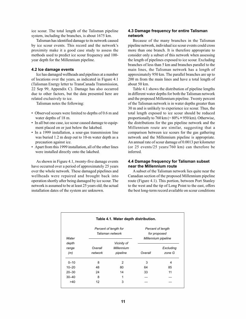
4.3 Damage frequency for entire Talismannetwork

Because of the many branches in the Talismanpipeline network, individual ice scour events could crossmore than one branch. It is therefore appropriate toconsider only a subset of this network when assessingthe length of pipelines exposed to ice scour. Excludingbranches of less than 5 km and branches parallel to themain lines, the Talisman network has a length ofapproximately 950 km. The parallel branches are up to200 m from the main lines and have a total length ofabout 50 km.

Table 4.1 shows the distribution of pipeline lengthsin different water depths for both the Talisman networkand the proposed Millennium pipeline. Twenty percentof the Talisman network is in water depths greater than30 m and is unlikely to experience ice scour. Thus, thetotal length exposed to ice scour should be reducedproportionally to 760 km (= 80% × 950 km). Otherwise,the distributions for the gas pipeline network and theMillennium route are similar, suggesting that acomparison between ice scours for the gas gatheringnetwork and the Millennium pipeline is appropriate.An annual rate of scour damage of 0.0013 per kilometer(or 25 events/25 years/760 km) can therefore beinferred.

4.4 Damage frequency for Talisman subsetnear the Millennium route

A subset of the Talisman network lies quite near theCanadian section of the proposed Millennium pipelineroute (Figure 4.1). This portion, between Port Stanleyto the west and the tip of Long Point to the east, offersthe best long-term record available on scour conditions

Table 4.1. Water depth distribution.

Percent of length for Percent of length

Talisman network for proposed

Water Millennium pipeline

depth Vicinity of

range Overall Millennium Excluding

(m) network pipeline Overall zone G

0–10 8 2 3 4

10–20 48 80 64 85

20–30 24 14 33 11

30–40 8 1 — —

>40 12 3 — —

11

along the Millennium route. The Talisman subset has alength of 309 km, excluding branches less than 5 km inlength and 42 km of parallel lines. The proportion of thelength is given as a function of water depth in Table 4.1.

Zone G of the Millennium pipeline (107–136 kmfrom Canadian landfall) is nearly 30 m deep and beyondthe water depth for scour damage. If this zone isexcluded, the depth distribution for the Talismannetwork is nearly identical to that for the proposedpipeline (Table 4.1). On this basis, it is appropriate tocompare damage rates for the Talisman network to scourrates over the Millennium pipeline.

From Figure 4.1, thirteen damage events occurredover a period of approximately 25 years in the Talismansubset near the proposed pipeline. An annual damagefrequency of 0.0017 per kilometer (13 events/25 years/309 km) can be inferred from these data.

4.5 Inference for scour frequency alongMillennium pipeline route

Some of the ice scours crossing the Talisman networkmay not have caused serious damage. Consequently theabove damage rates may underestimate the rate for allscours crossing over the network. However, this effectshould be small. It is unlikely that many of the scourswould have crossed the network of small-diameterpipelines without causing significant damage.

Another consideration is the orientation of scourswith respect to the pipeline. Many scour marks areobserved to be nearly parallel to the bathymetriccontours. For exact comparison of Talisman andMillennium scour frequencies, the orientation of theTalisman network segments and the Millenniumpipeline sections with respect to observed scour marksshould be considered. This correction has not been appliedto either data set; its effect should be less than 30%.

We therefore conclude that the damage rate inferredfrom the Talisman subset (0.0017 scours/km/yr)approximates the scour rate along the Canadian sectionof the Millennium route over the past 25 years. Basedon the 1998 CSR survey, C-CORE (1999a) estimatedthe scour rates in the Canadian zones (A–E) to be 0.10–0.44 scours/km/yr. These estimates are conservative byan order of magnitude compared to the Talisman subset.

Although directly applicable to the Canadian section,this comparison also provides confidence in the scourrates estimated by C-CORE (1999a) for the U.S. sectionof the Millennium route. It suggests that C-COREconservatively underestimated the scour ages from the1998 CSR data. On this basis, there is no reason tobelieve that annual scour frequencies should be anyhigher than originally recommended by C-CORE(1999a).

4.6 Inference for scour depth distributionTalisman reported that the deepest scour they have

observed was 0.6 m. If this was one of the 13 damageevents considered in Section 4.4, it provides anindependent estimate of the scour depth distributionalong the proposed Millennium route. This informationis used in Section 5.3.4 to assess the implications of theTalisman data on the design scour depths for theMillennium pipeline.

5.0 DESIGN SCOUR DEPTH

5.1 Strategy

5.1.1 Differences from C-CORE Report 98-C34C-CORE Report 98-34 (C-CORE 1999a) describes

the data and methods used to determine the 100-yearor design scour depths for each zone of the proposedMillennium pipeline. As noted in Section 2.2, themethod used parallels the method used to design theNorthstar oil pipeline for ice scour resistance.Nevertheless, to increase confidence in the design, C-CORE and ERDC researchers agreed to incorporateadditional data on Lake Erie scours and to conductadditional analyses. While the basic approach isidentical with C-CORE (1999a), the following changeshave been made:

• Only new scours have been considered.• Scour data from other comprehensive surveys near

the Millennium route have been included.• Scour rates were substantiated with data from the

Talisman gas-gathering network (Chapter 4).• An exponential distribution with a cutoff depth has

been used to account for under-sampled shallowscours.

• Several benchmarks have been used to validate thepredicted design scour depth.

5.1.2 Overview of new scour data for Lake ErieAs noted in Chapter 3, we chose to include only

“new” scours in the design analyses because these bestrepresent the population of scours as they are created.We also selected only data from comprehensive surveysnear the Millennium route and exposed to similar icescour conditions. This yielded the following datasources (Table 3.1): the 1981 and 1982 Ontario HydroCoho surveys, the 1995 USGS Ohio survey, and the1998 CSR Millennium pipeline route survey.

Tables 3.2 and 3.3 present the scour depth data usedhere. They represent the most comprehensive dataavailable that are appropriate to the design of theMillennium pipeline Lake Erie crossing.

12

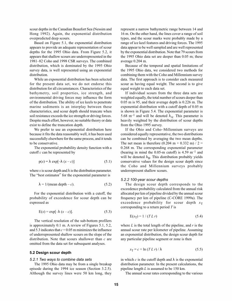
5.1.3 Scour depth distributionsFigure 5.1 shows the distribution of scour depths

for the 1995 USGS Ohio survey. Of the 96 measurednew scours, the maximum depth is 0.6 m. We usedWeibull plotting position (rank of the point indescending order divided by the total number of pointsplus one) to estimate the probability of exceedence formeasured scour depths. The exceedence plot is a semi-log scale, so that exponentially distributed scour depthswould plot as a straight line. The mean depth for theOhio data is 0.17 m, and the standard deviation is 0.13m. Since the standard deviation is less than the mean,an exponential fit would tend to predict slightly greaterprobabilities of occurrence for larger scour depths thanthe original data would indicate.

Figure 5.2 shows the scour depths from 1981–82Coho and the 1998 CSR surveys combined. The meanscour depth is 0.33 m, and the standard deviation is0.19 m. Of the 16 data points, the maximum scour depthis 0.7 m (an infilled scour on the pipeline route for whichthe original depth could be estimated). The histogramfor scour depth indicates that the data are poorlysampled. Note that the original 25 scour depthsmeasured along the Millennium route fit an exponential

distribution (C-CORE 1999a). The poor fit hereprobably reflects the small sample sizes from the twosurveys (new scours only).

Figure 5.3 shows the depth distribution of the threesurveys combined (112 points). The mean scour depthis 0.20 m, the standard deviation is 0.15 m, and themaximum scour depth is 0.7 m. The exceedence datashow a fairly linear trend below 0.05 m, with a slightdecrease for depths greater than 0.5 m. The combineddata set reflects the relatively good exponential fit ofthe large 1995 Ohio data set.

5.1.4 Probability distribution for scour depthThere is no unique probability distribution

characterizing the ice scour depths. The exponentialdistribution with a cutoff depth provides a reasonablefit to scour depths in the Alaskan Beaufort Sea (Weekset al. 1983, Wheeler and Wang 1985, INTEC 1998b).It appears to slightly overpredict the occurrence of deepscours, making it a conservative choice for predictingdesign scour depths. The cutoff depth relates to theresolution of the survey system and corrects the slopeof the distribution for undersampling of shallow scours.Weibull and gamma distributions yielded better fits to

Figure 5.1. Depth distribution of “new” scours compiled from 1995 OhioGeological Survey data.

13

Scour Depth (m)

Pro

bab

ility

of

Exc

eed

ance

Figure 5.2. Depth distribution of“new” scours compiled fromOntario Hydro 1981 and 1982surveys (Coho) and from CanadianSeabed Research 1998 routesurvey.

Figure 5.3. Depth distribution of“new” scours compiled from theOntario Hydro 1981 and 1982surveys (Coho), from the Ohio1995 survey, and from theCanadian Seabed Research 1998route survey.

14

Pro

bab

ility

of

Exc

eed

ance

Pro

bab

ility

of

Exc

eed

ance

Scour Depth (m)

Scour Depth (m)

scour depths in the Canadian Beaufort Sea (Nessim andHong 1992). Again, the exponential distributionoverpredicted deep scours.

Based on Figure 5.1, the exponential distributionappears to provide an adequate representation of scourdepths for the 1995 Ohio data. From Figure 5.2, itappears that shallow scours are underrepresented in the1981–82 Coho and 1998 CSR surveys. The combineddistribution, which is dominated by the 1995 Ohiosurvey data, is well represented using an exponentialdistribution.

While an exponential distribution has been selectedfor the present data set, we do not endorse thisdistribution for all circumstances. Characteristics of thebathymetry, soil properties, ice strength, andenvironmental driving forces may influence the formof the distribution. The ability of ice keels to penetratemarine sediments is an interplay between thesecharacteristics, and scour depth should truncate whensoil resistance exceeds the ice strength or driving forces.Despite much effort, however, no suitable theory or dataexist to define the truncation depth.

We prefer to use an exponential distribution herebecause it fits the data reasonably well, it has been usedsuccessfully elsewhere for the same process, and it tendsto be conservative.

The exponential probability density function with acutoff c can be represented by

p(x) = λ exp[–λ (x – c)] (5.1)

where x is scour depth and λ is the distribution parameter.The “best estimator” for the exponential parameter is

λ = 1/(mean depth – c). (5.2)

For the exponential distribution with a cutoff, theprobability of exceedence for scour depth can beexpressed as

E(x) = exp[–λ (x – c)]. (5.3)

The vertical resolution of the sub-bottom profilersis approximately 0.1 m. A review of Figures 5.1, 5.2,and 5.3 indicates that c = 0.05 m minimizes the influenceof underrepresented shallow scours on the slope of thedistribution. Note that scours shallower than c areomitted from the data set for subsequent analyses.

5.2 Design scour depth

5.2.1 Two ways to combine data setsThe 1995 Ohio data may be from a single breakup

episode during the 1994 ice season (Section 3.2.5).Although the survey lines were 50 km long, they

represent a narrow bathymetric range between 14 and16 m. On the other hand, the lines cover a range of soiltypes, and the scour marks were probably made by arange of ice keel features and driving forces. The 1995data appear to be well sampled and are well representedby the exponential distribution. Note that 79 scours fromthe 1995 Ohio data set are deeper than 0.05 m; theseaverage 0.204 m.

Because of the temporal and spatial limitations ofthe 1995 Ohio data, we considered two methods forcombining them with the Coho and Millennium surveydata. The first approach is to consider each measuredscour as having equal weight. The second is to giveequal weight to each data set.

If individual scours from the three data sets areweighted equally, the total number of scours deeper than0.05 m is 95, and their average depth is 0.226 m. Theexponential distribution with a cutoff depth of 0.05 mis shown in Figure 5.4. The exponential parameter is5.68 m–1 and will be denoted λA. This parameter isheavily weighted by the distribution of scour depthsfrom the Ohio 1995 survey.

If the Ohio and Coho–Millennium surveys areconsidered equally representative, the two distributionscan be combined by averaging the two mean depths.The net mean is therefore (0.204 m + 0.332 m) / 2 =0.268 m. The corresponding exponential parameter(bearing in mind the 0.05-m cutoff) is 4.59 m–1 andwill be denoted λB. This distribution probably yieldsconservative values for the design scour depth sincethe Coho and Millennium surveys probablyunderrepresent shallow scours.

5.2.2 100-year scour depthsThe design scour depth corresponds to the

exceedence probability calculated from the annual riskallocated per km of pipeline divided by the annual scourfrequency per km of pipeline (C-CORE 1999a). Theexceedence probability for scour depth xTcorresponding to a return period T is

E(xT) = 1 / (T L r) (5.4)

where L is the total length of the pipeline, and r is theannual scour rate per kilometer of pipeline. Assumingan exponential distribution, the design scour depth forany particular pipeline segment or zone is then

xT = c + ln (T L r) / λ (5.5)

in which c is the cutoff depth and λ is the exponentialdistribution parameter. In the present calculations, thepipeline length L is assumed to be 150 km.

The annual scour rates corresponding to the various

15

pipeline sections are listed in Table 5.1 for U.S. waters.C-CORE (1999a) based the rates for zones I and J onestimated residence times for scours recorded by the1998 CSR survey. Scour rates for zones where no scourswere observed (F, G, and H) were assigned values basedon other considerations (Section 3.3). Additional review(Section 3.3) and analysis of damage data for theTalisman network (Section 4.5) showed that the ratesin Table 5.1 are reasonable or conservative.

For equally weighted scours, the exponentialparameter is λA = 5.68 m–1. The design scour depth

Table 5.1. Millennium pipeline zones in U.S. waters defined in C-CORE(1999a).

Distance from Start–end Undrained AnnualCanadian water shear scour 100-year ice

Pipeline landfall depth range strength frequency scour depthzone (km) (m) (kPa) (/km) (m)

F 99–107 22.3–28.2 25 0.01 0.8*G 107–136 28.2–27.1 25 0.01 0.8*H 136–139 27.1–17.6 100 0.10 1.2I 139–146 17.6–18.3 100 0.11 1.2J 146–150 18.3–5.0 100 0.08 1.2

ALF 150–DDA Rock

ALF: American LandfallDDA: End of Directionally Drilled Pipe from American Landfall* Assigned values based on need to protect pipeline from anchors and fishing gear. Icescour does not control trench depths for zones F and G.

Figure 5.4. Exponentialfit to depth distributionof “new” scours com-piled from Ontario Hydro1981 and 1982 surveys(Coho), from Ohio Geo-logical Survey 1995survey, and from Cana-dian Seabed Research1998 route survey.

corresponding to a 100-year return period is 0.93 m forsections F and G, and 1.34 m for zones H, I, and J. Asstated in the last section, this approach tends to bias theresults in favor of the 1995 Ohio data, which form thelargest portion of the data set.

For equally weighted data sets (1995 Ohio surveyand 1981–82 Coho/1998 CSR surveys), the exponentialparameter is λB = 4.59 m–1. The design scour depthcorresponding to a 100-year return period is 1.14 m forzones F and G, and 1.64 m for zones H, I, and J. Asnoted, this approach is probably conservative.

16

Scour Depth (m)

Pro

bab

ility

of

Exc

eed

ance

It is tempting to select the more conservative of thetwo results for design. However, use of an exponentialdistribution already introduces conservatism inpredicted design scour depths (Section 5.1.4).Furthermore, codes for marine pipelines (ASME 1995,CSA 1999) allow for the random nature ofenvironmental loads by specifying return periods muchlonger than the service life of the pipeline. These codesspecify designing for expected 100-year events, withoutspecifying reliability levels or safety factors. Weinterpret them as specifying a “best estimate” (i.e., 50%reliable estimate) of the 100-year event.

Our “best estimate” of the 100-year scour depth inzones H, I, and J is the average of the results from thetwo methods described above: x100 = (1.34 + 1.64) =1.49 m = 1.5 m. Note that all scours used to determinethe depth distribution and rates derive from surveysalong the Millennium route or in areas of similar icescour conditions to zones H–J.

Zones F and G must be handled differently. Neitherthe 1997 Racal survey nor the higher-resolution 1998CSR survey revealed any evidence of ice scour in zonesF and G. Consequently C-CORE (1999a) arbitrarilyassigned a rate of 0.01 scours/km/yr for these zones,essentially to protect the pipeline from dragging anchorsand fishing gear. With their original scour-depthdistribution (exponential with no cutoff, l = 6.2 m–1),they calculated x100 = 0.8 m. This depth plus allowancefor sub-scour deformation (0.1 m) seemed more thanadequate to protect the pipeline from these effects (C-CORE 1999a).

The 1998 CSR survey should have revealed evidenceof scour over at least the past 50 years (Section 3.3.1).Using equation (5.5), we may calculate the scour rate

Table 5.2. Revised 10-year and 100-year scour depths for Millennium pipelinezones in U.S. waters. Note adjustments to the zone locations and depth ranges.

Distance from Start–end Annual 10-year 100-year

Canadian water scour scour scour

Pipeline landfall depth range frequency depth depth

zone (km) (m) (/km) (m) (m)

F 98.0–105.0 21.0–26.7 0.01 0.3–0.6 0.8*G 105.0–135.1 26.7–27.4 0.01 0.3–0.6 0.8*H 135.1–136.8 27.4–18.4 0.10 1.0 1.5I 136.8–142.2 18.4–16.4 0.11 1.0 1.5J 142.2–147.3 16.4–17.1 0.08 1.0 1.5

ALF 147.3–149.3 (DDA) 17.1–8.3

ALF—American LandfallDDA—End of Directionally Drilled Pipe from American Landfall* Assigned values based on need to protect pipeline from anchors and fishing gear. Ice scourdoes not control trench depths for zones F and G.

inferred by choosing x100 = 0.8 m and check it forconsistency. For λA = 5.68 m–1 , r ~ 0.005 scours/km/yr, and for λB = 4.59 m–1 , r ~ 0.002 scours/km/yr. ZonesF and G are about 37 km long. Thus, if the lakebedpreserves a 50-year scour record, the survey would haverevealed evidence of about 4–9 scours. Furthermore,the inferred rates equal or exceed the scour rate determinedfrom the Talisman damage data (Chapter 4).

We see no reason to alter C-CORE’s (1999a) designscour depth for zones F and G. Ice scour does not controlpipeline trench depth in zones F and G, and x100 = 0.8 mprovides a reasonable level of protection even if it did.

Table 5.2 summarizes the revised design scour depthsfor the U.S. section of the proposed Millennium pipelineroute.

5.2.3 U.S. landfallThe landfall area adjacent to the U.S. shore (denoted

ALF in C-CORE 1999a) consists primarily of bedrock.Ice scour is not an issue in this material.

In the U.S. landfall area, it is recommended that thepipe crown be placed flush with the lakebed allowingfor pipe curvature over changes in the slope of thetrench. To ensure this, the trench should be at least 1064mm deep, accounting for the 914-mm outside diameterof the pipe and 150 mm to account for the 75-mmconcrete cover.

5.3 Sensitivity and benchmark analyses

5.3.1 Sensitivity to exponential cutoff valueThe value selected for the cutoff in the exponential

scour-depth distribution, c = 0.05 m, fits the data well(Figures 5.1–5.4). It is also consistent with a sub-bottomprofiler resolution of about 0.1 m. We examined the

17

sensitivity of the 100-year scour depths predicted forzones H–J to variations in c. Using the methods inSection 5.2.2, we would expect x100 = 1.64 m for c = 0,and x100 = 1.31 for c = 0.10 m. Thus, the expected 100-year scour depths are not highly sensitive to c, and theiraverage agrees with our best estimate of x100 = 1.5 m.

5.3.2 Predicted 10-year scour depthsThe record of observed scours in Lake Erie is much

less than 100 years. Thus, it is instructive to predict 10-year scour depths for the different pipeline zones. Forzones H, I, and J, x10 = 1.0 m based on the methods inSection 5.2.2. This is reasonable considering that thedeepest scour in the data set analyzed is 0.7 m (Section5.1.3).

The expected 10-year scour depth in zones F and Gdepends on the rate assigned: x10 ~ 0.3 m for r = 0.002scours/km/yr, and x10 ~ 0.6 m for r = 0.01 scours/km/yr. The 1998 CSR survey would certainly have detectedscours this deep had they been present. It appears thateven the lower scour rate is conservative.

5.3.3 Isolated deep scoursThe scour data set used for design included only

scour depths from comprehensive surveys (Section 3.2).Nevertheless, isolated deep scours have been observedin Lake Erie (Section 3.4). In particular, the Kozak scourmeasured 1 m deep, and the ice island scour measured1.5 m deep. Based on our best estimates for zones H, I,and J, these scours correspond to 10-year and 100-yearevents, respectively.

Inclusion of these isolated deep scours does not affectthe best estimates for the 100-year scour depths. Thedesign database would include 97 (equally weighted)scours deeper than 0.05 m. The resulting mean valueof 0.247 m yields λA = 5.09 m–1 and x100 = 1.49 m (forr = 0.1 scours/km/yr). Although this is higher than thevalue based on the 95 equally weighted scours fromcomprehensive surveys (x100 = 1.34 m), the effect isexaggerated. Many small scours should accompanyeach deep scour if they derive from the same processas the other data sets. Indeed, the method using equallyweighted data sets cannot be used with isolated scoursfor this reason. Consequently the expected 100-yearscour depth including the two deep scours agrees withour best estimate, x100 = 1.5 m.

5.3.4 Talisman dataThe damage records for the Talisman gas network

represent the longest record available on ice scour inLake Erie (Chapter 4). Thirteen breakages due to icescour occurred in the network subset near theMillennium route over a 25-year period. If the deepestscour observed by Talisman (0.6 m) was one of these

13, its exceedence probability based on Weibull plottingposition would be E(0.6 m) ~ 1 – 13/14 = 0.0714.Assuming an exponential depth distribution with c =0.05 m, equation 5.3 yields λ = 4.8 m–1. This value ofλ agrees well with those from the design data set(Section 5.2.2) and would predict x100 = 1.6 m for r =0.1 scours/km/yr (zones H–J). Within the uncertaintyof the Talisman calculation, this agrees with our bestestimate (x100 = 1.5 m).

The Talisman benchmark directly applies toCanadian zones of the Millennium pipeline. Theinferred scour rate, ~ 0.002 scours/km/yr, isconservative by an order of magnitude compared withthe estimates for the pipeline zones A–E (Section 4.5).If the scour rate is approximately constant, we wouldexpect 4 × 13 = 52 scours in 100 years based on theTalisman data. Consequently equation 5.5 wouldsuggest x100 = 0.05 + ln (52 + 1)/4.8 = 0.88 m = 0.9 m.This is significantly less than C-CORE’s (1999a) designdepths for the Canadian section (1.2–1.4 m).

C-CORE used the same method to estimate scourrates in U.S. zones H, I, and J (0.08–0.11). The Talismandata suggest these rates could also be conservative,although ice exposure conditions differ. Nevertheless,our best estimate x100 = 1.5 m provides sufficient marginfor uncertainty in scour rates in these zones.

5.3.5 1998 route data adjusted for infill effectData from the Beaufort Sea indicate that new scours

may be about 20% deeper on average than existingscours, although they approximate the same distribution(Section 3.2.1). C-CORE (1999a) originally calculateddesign scour depths for the Millennium route based on25 scour depths (new and infilled) measured along theroute by the 1998 CSR survey. The average depth was0.166 m. The Beaufort Sea data suggest that we mayapproximate the average depth of the new scours thatformed this distribution by applying a 20% correctionfor infilling, 0.166 × 1.2 ~ 0.20 m.

C-CORE found that an exponential distribution withc = 0 fit the measured depths reasonably well. Usingthe adjusted mean depth, the distribution parameterwould be λ = 1/0.20 = 5.0 m–1. Thus, in pipeline zonesH–J (r = 0.1 scours/km/yr) the C-CORE’s originallyused distribution adjusted for infilling would yield x100= 1.5 m (equation 5.5). This is coincidental agreementwith our best estimate, but it does suggest that the infilleffect in Lake Erie is also small on average.

5.3.6 100-year scour depth for 1994-like episodesThe new scours recorded by the USGS 1995 Ohio

survey may have derived from a single breakup episodein 1994 (Section 3.2.5). These scours occurred in waterdepth, soil, and ice exposure conditions similar to

18

pipeline zone J. We may estimate the 100-year scourdepth for 1994-like episodes and compare it to the best-estimate value for zone J.

The 1995 Ohio data set consists of 79 scours deeperthan 0.05 m found along 50 km of survey lines, or 1.6scours/km-line. These scours were primarily parallelto shore and intersected the survey lines at shallowangles. Assuming an average intersection angle of 15degrees, the scour density across a pipelineperpendicular to the average scour direction would beapproximately six scours/km.

The recurrence interval for 1994-like events is moredifficult to estimate. Fortunately the expected 100-yearscour depth is insensitive to recurrence interval.

Assel et al. (1996) found that the winter temperaturesmeasured around Lake Erie rank 1994 about the 18thcoldest of 97 years of record. This suggests a returnperiod for ice conditions of about five years. However,Assel et al. (1996) report that gale force winds on 14March 1994 caused considerable ice ridging. That is,ice and high winds probably caused the ice scourepisode, and their lower joint probability would suggesta recurrence interval longer than five years. Also, the1998 CSR survey found no high-density 1994-likescours. Based on their appearance class, C-CORE(1999a) estimated the scours observed to be about 7.5years old.

Our best estimate for the recurrence interval for1994-like events is about 10 years. The resulting scourrate over a pipeline perpendicular to the scour directionwould be r ~ 6 scours/km/10 years = 0.6 scours/km/yr.The scour depth distribution for the 1995 Ohio data(Fig. 5.1) yields λ = 6.48 m–1 for c = 0.05 m. Theexpected 100-yr scour depth from equation 5.5 is x100= 1.45 m = 1.5 m. Varying the estimated recurrencerate for 1994-like episodes from five to 10 years variesthe expected 100-year scour depth from 1.4 to 1.6 m.The result is also not sensitive to other variablesaffecting r, and the exponential distribution tends to beconservative for deep scours. Thus, our best estimateof x100 = 1.5 m for zone J is reasonable.

5.4 Summary of revisions to design scourdepth

There are two significant differences in the data usedto obtain the present results compared with original C-CORE analysis. First, only “new” scour features, withno significant infilling, have been considered. Second,the data set used for design analyses has been expandedto include depth measurements for approximately 100scours from the 1995 USGS Ohio survey and from the1981–82 Ontario Hydro Coho surveys.

We used two methods to combine the data andselected our “best estimate” of the 100-year scour depth

as the average of the resulting two values. Where scourcontrols the design depth (pipeline zones H–J), our bestestimate x100 = 1.5 m compares well with severalbenchmark calculations. As a result of this work, thereis significantly more confidence in the present designscour depths for the Millennium pipeline.

6.0 PIPE RESPONSE AND TRENCH DEPTH

6.1 IntroductionThe response of the Millennium pipeline to ice scour

(gouge) events was analyzed by a finite-elementnumerical model. The ice scour events are based on the100-year design scour depths presented in Section 5.2.The trench depths for the pipeline were assessed so thatresulting longitudinal pipe strains did not exceed tensileor compressive design limits.

Section 5.2 of C-CORE (1999a) describes in detailthe stress-based and strain-based designs applied to theMillennium pipeline. The design limits were based oncode recommendations (CSA 1999) and discussionswith Millennium partner Trans-Canada Pipelines. Thedesign tensile strain limit of 2.5% generally governsthe required trench depth. It is important to note thatthese limits are for safe operation. It is expected thatthe pipe failure strain to rupture will be about 3.75%,representing a factor of safety of about 1.5.

This chapter briefly describes the model used, theresults of the ERDC review of the model, and the designtrench depths based on revised 100-year scour depths.Also included is a brief description of conservatism inthe analyses.

6.2 Pipe-response model overviewThe response of the Millennium pipeline subject to

ice scour events was analyzed by a finite-elementnumerical model. This model is described in Section 5and Appendix B of C-CORE (1999a) and is presentedin Kenny et al. (2000). This numerical model comprisedthree components: soil/pipeline interaction, ice scour/soil relationships, and finite-element formulation. Thissection briefly describes these components.

The soil/pipeline interaction model is based on ASCE(1984) guidelines for the seismic design of oil and gaspipeline systems. The idealized structural model isillustrated in Figure 6.1. The continuum soil responseis approximated by a series of discrete springs. Thestiffness terms, t-s and p-y, represent the axial andhorizontal soil response components, respectively. Theultimate or yield conditions were based on the ASCE(1984) guidelines.

The importance of sub-scour deformations wasrealized through the Pressure Ridge Ice Scour

19

Experiment (PRISE) investigations. Schematicillustrations of sub-scour deformation profiles areillustrated in Figures 6.2 and 6.3i. Details of theempirical relationships defining the sub-scourdisplacement field are presented in Woodworth-Lynaset al. (1996). The response functions were derived fromanalysis of centrifuge modeling tests conducted underPRISE. The longitudinal distribution (Fig. 6.2) ischaracterized by a bounded, peak central displacementwith a cosine tail distribution. The free-field verticalprofile under point B in Figure 6.3i exhibits anexponential decay with increasing depth.

In PRISE, an engineering model was developed toassess the influence of ice gouge events on buried

marine pipelines. This engineering model was used todesign the Northstar pipeline against ice scour (C-CORE 1999b). An improved version of this model wasused in the design of the pipeline for the Lake Eriecrossing. Pipeline response to subgouge soildeformations is modeled by fully nonlinear finite-element analysis using two-dimensional pipe elementscoupled to discrete soil springs. The effects of internalpressure, ice bearing pressure, and ice scour width anddepth on the longitudinal strain response of a buriedpipeline are all considered.

The finite-element analyses were conducted usingABAQUS/Standard. The soil/pipeline interaction model(Fig. 6.1) was discretized by two-dimensional beam

Figure 6.2. Plan view of the horizontal profile sub-scour soil displacement.

Figure 6.1. Schematic of finite-element model and geometric boundarycondition.

20

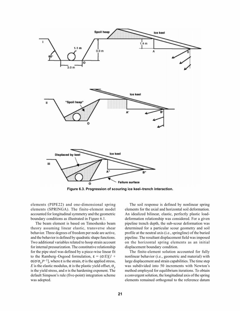
elements (PIPE22) and one-dimensional springelements (SPRINGA). The finite-element modelaccounted for longitudinal symmetry and the geometricboundary conditions as illustrated in Figure 6.1.

The beam element is based on Timoshenko beamtheory assuming linear elastic, transverse shearbehavior. Three degrees of freedom per node are active,and the behavior is defined by quadratic shape functions.Two additional variables related to hoop strain accountfor internal pressurization. The constitutive relationshipfor the pipe steel was defined by a piece-wise linear fitto the Ramberg–Osgood formulation, ε = (σ/E)[1 +α(σ/σy)n–1], where ε is the strain, σ is the applied stress,E is the elastic modulus, α is the plastic yield offset, σyis the yield stress, and n is the hardening exponent. Thedefault Simpson’s rule (five-point) integration schemewas adopted.

The soil response is defined by nonlinear springelements for the axial and horizontal soil deformation.An idealized bilinear, elastic, perfectly plastic load-deformation relationship was considered. For a givenpipeline trench depth, the sub-scour deformation wasdetermined for a particular scour geometry and soilprofile at the neutral axis (i.e., springline) of the buriedpipeline. The resultant displacement field was imposedon the horizontal spring elements as an initialdisplacement boundary condition.

The finite-element solution accounted for fullynonlinear behavior (i.e., geometric and material) withlarge displacement and strain capabilities. The time stepwas subdivided into 50 increments with Newton’smethod employed for equilibrium iterations. To obtaina convergent solution, the longitudinal axis of the springelements remained orthogonal to the reference datum

Figure 6.3. Progression of scouring ice keel–trench interaction.

21

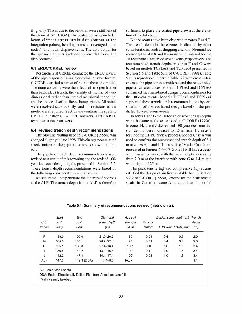
(Fig. 6.1). This is due to the zero transverse stiffness ofthe element (SPRINGA). The post-processing includedbeam element stress–strain data (output at theintegration points), bending moments (averaged at thenodes), and nodal displacements. The data output forthe spring elements included centroidal force anddisplacement.

6.3 ERDC/CRREL reviewResearchers at CRREL conducted the ERDC review

of the pipe response. Using a question–answer format,C-CORE clarified a series of points about the model.The main concerns were the effects of an open (ratherthan backfilled) trench, the validity of the use of two-dimensional rather than three-dimensional modeling,and the choice of soil stiffness characteristics. All pointswere resolved satisfactorily, and no revisions to themodel were required. Section 6.6 contains the specificCRREL questions, C-CORE answers, and CRRELresponse to those answers.

6.4 Revised trench depth recommendationsThe pipeline routing used in C-CORE (1999a) was

changed slightly in late 1998. This change necessitateda redefinition of the pipeline zones as shown in Table6.1.

The pipeline trench depth recommendations wererevised as a result of this rezoning and the revised 100-year ice scour design depths presented in Section 5.2.These trench depth recommendations were based onthe following considerations and analyses.

Ice scours will not penetrate the outcrop of bedrockat the ALF. The trench depth in the ALF is therefore

sufficient to place the coated pipe crown at the eleva-tion of the lakebed.

No ice scours have been observed in zones F and G.The trench depth in these zones is dictated by otherconsiderations, such as dragging anchors. Nominal icescour depths of 0.8 and 0.4 m were considered for the100-year and 10-year ice scour events, respectively. Therecommended trench depths in zones F and G werebased on models TCPLes3 and TCPLes4 presented inSection 5.6 and Table 5.11 of C-CORE (1999a). Table5.11 is reproduced in part in Table 6.2 with cross-refer-ences to the pipe zones considered and the related steelpipe crown clearances. Models TCPLes1 and TCPLes3confirmed the strain-based design recommendations forthe 100-year events. Models TCPLes2 and TCPLes4supported these trench depth recommendations by con-sideration of a stress-based design based on the pre-dicted 10-year scour events.

In zones F and G the 100-year ice scour design depthswere the same as those assessed in C-CORE (1999a).In zones H, I, and J the revised 100-year ice scour de-sign depths were increased to 1.5 m from 1.2 m as aresult of the EDRC review process. Model Case X wasused to confirm the recommended trench depth of 3.4m in zones H, I, and J. The results of Model Case X arepresented in Figures 6.4–6.7. Zone H will have a deep-water transition zone, with the trench depth increasingfrom 2.0 m at the interface with zone G to 3.4 m at awater depth of 25 m.

The peak tensile (εt) and compressive (εc) strainssatisfied the design strain limits established in Section5.2.2 of C-CORE (1999a), except for the peak tensilestrain in Canadian zone A as calculated in model

Table 6.1. Summary of recommendations revised (metric units).

Start End Start-end Avg soil Design scour depth (m) Trench

U.S. pos’n pos’n water depth strength Scours depth

zones (km) (km) (m) (kPa) /km/yr 1:10 year 1:100 year (m)

F 98.0 105.0 21.0–26.7 25 0.01 0.4 0.8 2.0

G 105.0 135.1 26.7–27.4 25 0.01 0.4 0.8 2.0

H 135.1 136.8 27.4–18.4 100* 0.10 1.0 1.5 3.4

I 136.8 142.2 18.4–16.4 100* 0.11 1.0 1.5 3.4

J 142.2 147.3 16.4–17.1 100* 0.08 1.0 1.5 3.4

ALF 147.3 149.3 (DDA) 17.1–8.3 Rock 1.1

ALF: American Landfall

DDA: End of Directionally Drilled Pipe from American Landfall

*Mainly sandy lakebed

22

TCPLes1. The calculated axial tensile strain in zone A(2.6%) slightly exceeds the allowable limit of 2.5%.This calculated value will be reduced by the presenceof the open trench to within acceptable values.

6.5 Model conservatismThe pipe-response model includes two sources of

conservatism. First, the model assumes that ice keelstransfer loads to the pipe through intact native soil. Infact, the Millennium pipeline will lay in an open trenchthat will backfill naturally over a period of years. Thestrength of this backfill material will be significantlyless than that of intact native soil. Consequently theloads that this material will transfer from a scouringice keel to the pipeline, and the resulting pipeline strains,will be less than the model calculates (see response to

question 2 in Section 6.6). Modeling limitationsprevented quantifying this effect, but it should besignificant.

Second, all design calculations are based on a normalangle of incidence of the ice keel relative to the pipeline(Fig. 6.2). This is a worst-case scenario. Section 5.5 ofC-CORE (1999a) reported strains calculated by thepipe-response model for 0-, 30-, and 45-degreeincidence angles for a 1-m-deep, 14-m-wide scour. Forsoil strengths where ice scour governs the design (50–100 kPa), the calculated pipe strains decreased by 20%at 30-degree incidence and 40% at 45-degree incidence.For random scour directions, 45 degrees would be themost likely incidence angle. However, the scour surveysare not sufficiently extensive to determine the averageorientation of scours relative to the pipeline orientation.

Table 6.2. Models supporting trench depth recommendations.

Scour Scour Trench

Model Cu width depth Peak εt Peak εc depth Clearance

(#) Zone (kPa) (m) (m) (%) (%) (m) (m)

Case X H,I,J 100 14 1.5 2.4 –0.8 3.4 0.8

TCPLes1 A 100 14 1.4 2.6 –0.9 2.9 0.5

TCPLes 2 A 100 14 1.0 1.2 –0.7 3.0 1.0

TCPLes 3 F,G 25 14 0.8 0.45 –0.3 2.0 0.2

TCPLes 4 F,G 25 14 0.4 0.14 –0.1 1.9 0.5

Figure 6.4. Transverse horizontal load-displacement relationship (symmetric) for Case X.

23

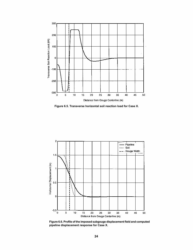
Figure 6.5. Transverse horizontal soil reaction load for Case X.

Figure 6.6. Profile of the imposed subgouge displacement field and computedpipeline displacement response for Case X.

24

Consequently this effect was not incorporated into thedesign trench depths.

6.6 Responses to specific ERDC reviewquestions

In this section, original questions by CRREL aregiven in italic font, C-CORE responses to thesequestions follow “C-CORE:,” and CRREL commentson the C-CORE responses follow “CRREL:.” CRRELhad no follow-up questions for C-CORE. The figuresand references in the original correspondence have beenupdated to figures and references contained in thisreport.

1. Chapter 5 of the February 1999 C-CORE FinalReport “Lake Erie Ice Scour/Pipeline Design” (C-CORE 1999a) does not make it clear that the PRISEapproach for designing buried pipelines is adaptableor appropriate to the problem of a pipeline in an un-backfilled trench, although assumptions regardinginfilling over time and during a scour event have beendescribed and used. Specifically, is the prescribedboundary condition determined from the PRISEcentrifuge experiments (presumably conducted withouta trench configuration) appropriate for an un-backfilledtrench, or even for a trench that has filled in over time?How would the design be affected if the boundarycondition were not appropriate? If the boundarycondition is appropriate, then a clarifying discussionof the analysis’ assumptions regarding infilling overtime and during a scour event, particularly how these

effects bring the calculated stress values “to withinacceptable levels” (as stated in C-CORE 1999a, Section5.6), would be helpful to our understanding.

C-CORE: The PRISE experiments did not include anypipe sections. These experiments were used todetermine only scour forces and sub-scour soildisplacement relationships in the absence of any otherstructures (e.g., pipelines or infilled trenches). (C-COREhas conducted some proprietary centrifuge tests ofscour–soil–pipe interaction.)

The interaction of these sub-scour soil displacementswith the pipeline was assessed through a pipe–soilinteraction analysis. This decoupling of the ice–soilfrom soil–pipe interaction is common in pipelineengineering. For example, the same principle is adoptedfor pipelines crossing moving slopes, where the slopeanalysis for movements is decoupled from the soilmovement–pipe interaction analysis.

In the pipe–soil interaction analysis, the lateralinteraction of the soil with the pipe is modeled by thep-y springs. The response of these springs shows howincreasing the relative movement of the pipe to the soilchanges the lateral pressure acting on the pipe. It wasassumed in the analysis that the pipe interacted directlywith the native soil (that is, the presence of a partlyinfilled trench was ignored). This direct interaction wasconsidered to provide a reasonable upper bound to thelateral pressures (p) acting on the pipe, which in turncauses the maximum flexural strains in the pipe. Section5.4 of the report considered the effect of a trench around

Figure 6.7. Longitudinal distribution of axial strain for Case X.

25

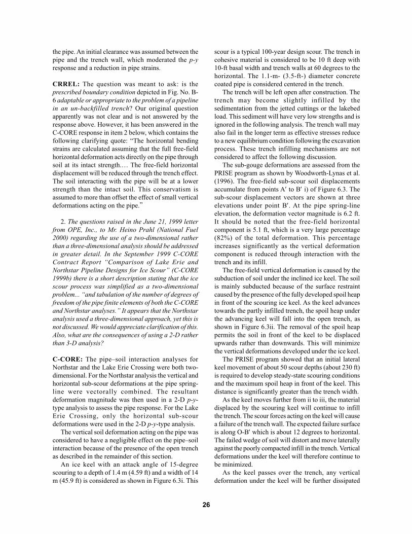
the pipe. An initial clearance was assumed between thepipe and the trench wall, which moderated the p-yresponse and a reduction in pipe strains.

CRREL: The question was meant to ask: is theprescribed boundary condition depicted in Fig. No. B-6 adaptable or appropriate to the problem of a pipelinein an un-backfilled trench? Our original questionapparently was not clear and is not answered by theresponse above. However, it has been answered in theC-CORE response in item 2 below, which contains thefollowing clarifying quote: “The horizontal bendingstrains are calculated assuming that the full free-fieldhorizontal deformation acts directly on the pipe throughsoil at its intact strength.… The free-field horizontaldisplacement will be reduced through the trench effect.The soil interacting with the pipe will be at a lowerstrength than the intact soil. This conservatism isassumed to more than offset the effect of small verticaldeformations acting on the pipe.”

2. The questions raised in the June 21, 1999 letterfrom OPE, Inc., to Mr. Heino Prahl (National Fuel2000) regarding the use of a two-dimensional ratherthan a three-dimensional analysis should be addressedin greater detail. In the September 1999 C-COREContract Report “Comparison of Lake Erie andNorthstar Pipeline Designs for Ice Scour” (C-CORE1999b) there is a short description stating that the icescour process was simplified as a two-dimensionalproblem... “and tabulation of the number of degrees offreedom of the pipe finite elements of both the C-COREand Northstar analyses.” It appears that the Northstaranalysis used a three-dimensional approach, yet this isnot discussed. We would appreciate clarification of this.Also, what are the consequences of using a 2-D ratherthan 3-D analysis?

C-CORE: The pipe–soil interaction analyses forNorthstar and the Lake Erie Crossing were both two-dimensional. For the Northstar analysis the vertical andhorizontal sub-scour deformations at the pipe spring-line were vectorally combined. The resultantdeformation magnitude was then used in a 2-D p-y-type analysis to assess the pipe response. For the LakeErie Crossing, only the horizontal sub-scourdeformations were used in the 2-D p-y-type analysis.

The vertical soil deformation acting on the pipe wasconsidered to have a negligible effect on the pipe–soilinteraction because of the presence of the open trenchas described in the remainder of this section.

An ice keel with an attack angle of 15-degreescouring to a depth of 1.4 m (4.59 ft) and a width of 14m (45.9 ft) is considered as shown in Figure 6.3i. This

scour is a typical 100-year design scour. The trench incohesive material is considered to be 10 ft deep with10-ft basal width and trench walls at 60 degrees to thehorizontal. The 1.1-m- (3.5-ft-) diameter concretecoated pipe is considered centered in the trench.

The trench will be left open after construction. Thetrench may become slightly infilled by thesedimentation from the jetted cuttings or the lakebedload. This sediment will have very low strengths and isignored in the following analysis. The trench wall mayalso fail in the longer term as effective stresses reduceto a new equilibrium condition following the excavationprocess. These trench infilling mechanisms are notconsidered to affect the following discussion.

The sub-gouge deformations are assessed from thePRISE program as shown by Woodworth-Lynas et al.(1996). The free-field sub-scour soil displacementsaccumulate from points A′ to B′ i) of Figure 6.3. Thesub-scour displacement vectors are shown at threeelevations under point B′. At the pipe spring-lineelevation, the deformation vector magnitude is 6.2 ft.It should be noted that the free-field horizontalcomponent is 5.1 ft, which is a very large percentage(82%) of the total deformation. This percentageincreases significantly as the vertical deformationcomponent is reduced through interaction with thetrench and its infill.

The free-field vertical deformation is caused by thesubduction of soil under the inclined ice keel. The soilis mainly subducted because of the surface restraintcaused by the presence of the fully developed spoil heapin front of the scouring ice keel. As the keel advancestowards the partly infilled trench, the spoil heap underthe advancing keel will fall into the open trench, asshown in Figure 6.3ii. The removal of the spoil heappermits the soil in front of the keel to be displacedupwards rather than downwards. This will minimizethe vertical deformations developed under the ice keel.

The PRISE program showed that an initial lateralkeel movement of about 50 scour depths (about 230 ft)is required to develop steady-state scouring conditionsand the maximum spoil heap in front of the keel. Thisdistance is significantly greater than the trench width.

As the keel moves further from ii to iii, the materialdisplaced by the scouring keel will continue to infillthe trench. The scour forces acting on the keel will causea failure of the trench wall. The expected failure surfaceis along O-B′ which is about 12 degrees to horizontal.The failed wedge of soil will distort and move laterallyagainst the poorly compacted infill in the trench. Verticaldeformations under the keel will therefore continue tobe minimized.

As the keel passes over the trench, any verticaldeformation under the keel will be further dissipated

26

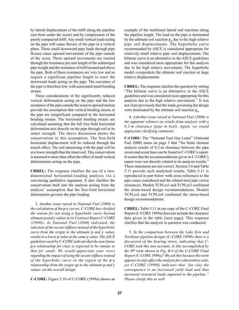
by lateral displacement of the infill along the pipeline(out from under the scour) and by compression of thepoorly compacted infill. Any small vertical loads actingon the pipe will cause flexure of the pipe in a verticalplane. These small downward pipe loads through pipeflexure cause upward movements of the pipe outsideof the scour. These upward movements are reactedthrough the resistance per unit length of the submergedpipe weight and the resistance of infill around and abovethe pipe. Both of these resistances are very low and sorequire a significant pipeline length to react thedownward loads acting on the pipe. The curvature ofthe pipe is therefore low, with associated small bendingstrains.

These considerations of the significantly reducedvertical deformation acting on the pipe and the lowresistance of the pipe outside the scour to upward motionprovide the assumption that vertical bending strains inthe pipe are insignificant compared to the horizontalbending strains. The horizontal bending strains arecalculated assuming that the full free-field horizontaldeformation acts directly on the pipe through soil at itsintact strength. The above discussion shows theconservatism in this assumption. The free-fieldhorizontal displacement will be reduced through thetrench effect. The soil interacting with the pipe will beat a lower strength than the intact soil. This conservatismis assumed to more than offset the effect of small verticaldeformations acting on the pipe.

CRREL: The response clarifies the use of a two-dimensional horizontal-loading analysis via aconvincing qualitative argument. It also clarifies theconservatism built into the analysis arising from theanalysis’ assumption that the free-field horizontaldeformation governs the pipe loading.

3. Another issue raised in National Fuel (2000) isthe calculation of the p-y curves. C-CORE has clarifiedthe reason for not using a hyperbolic curve beyondultimate p and y values in its Contract Report C-CORE(1999b). As National Fuel (2000) indicated, theselection of the secant stiffness instead of the hyperboliccurve from the origin to the ultimate p and y valuesresults in a lower p value at the same y value. The ASCEguidelines used by C-CORE indicate that the non-linearp-y relationship for clays is expected to be similar tothat for sands. We would appreciate your viewsregarding the impact of using the secant stiffness insteadof the hyperbolic curve–in the region of the p-yrelationship from the origin up to the ultimate p and yvalues–on the overall design.

C-CORE: Figure 5.10 of C-CORE (1999a) shows an

example of the mobilized lateral soil reactions alongthe pipeline length. The load on the pipe is dominatedby the ultimate soil reaction pu due to the high relativepipe soil displacements. The hyperbolic curverecommended by ASCE is considered appropriate forrelatively small relative pipe–soil displacements. Thebilinear curve is an alternative in the ASCE guidelinesand was considered more appropriate for this analysisdue to the high relative movements. The hyperbolicmodel overpredicts the ultimate soil reaction at largerelative displacements.

CRREL: The response clarifies the question by stating“The bilinear curve is an alternative in the ASCEguidelines and was considered more appropriate for thisanalysis due to the high relative movements.” It wasnot clear previously that the loads governing the designwere dominated by the ultimate soil reaction pu.

4. A further issue raised in National Fuel (2000) isthe apparent reliance on results from analysis with a0.2-m clearance (pipe to keel). Again, we wouldappreciate clarifying comments.

C-CORE: The “National Fuel Gas Letter” (NationalFuel 2000) states on page 3 that “No finite elementanalysis results of 0.2-m clearance between the pipecrown and scour base can be found in C-CORE’s report.It seems that the recommendations given in C-CORE’sreport were not directly related to its analysis results.”These statements are not correct. Section 5.6 and Table5.11 provide such analytical results. Table 5.11 isreproduced in part below with cross references to thepipe zones considered and the related steel pipe crownclearances. Models TCPLes1 and TCPLes3 confirmedthe strain-based design recommendations. ModelsTCPLes2 and TCPLes4 confirmed the stress-baseddesign recommendations.

CRREL: Table 5.11 in our copy of the C-CORE FinalReport (C-CORE 1999a) does not include the clearancedata given in the table [next page]. This responseclarifies that the analysis in question was conducted.

5. In the comparison between the Lake Erie andNorthstar pipeline designs (C-CORE 1999b) there is adiscussion of the bearing stress, indicating that C-CORE took this into account. Is this accomplished bythe H* term shown in Fig. B-4 of the C-CORE FinalReport (C-CORE 1999a)? We ask this because this termappears to only affect the analysis for cohesionless soils,yet C-CORE (1999b) indicates that “for clay theconsequence is an increased yield load and thusincreased structural loads imparted to the pipeline.”Please clarify this as well.

27

C-CORE: Figure 5.10 of C-CORE (1999a) shows theeffect of the bearing stress on the ultimate soil reactionspu inside and outside of the scour. The H* term is thedepth of burial equivalent to the addition of the verticalice bearing stress. This H* term (instead of H) in FigureB-9 is used to calculate the bearing capacity factor, Nc.The change in Nc reflects the change in failuremechanism of the pipe–soil system under the restraintof the ice keel. The H* term is NOT used to calculatethe yield displacement, yu, under the ice keel. The secantstiffness of the p-y curve under the scour is taken to bethe same as that outside of the scour.

CRREL: That C-CORE used the H* term to calculateNc answers the question.

6. Also in C-CORE (1999b) there is a discussion ofthe effect of the temperature change from pipeinstallation to operation, yet it is not indicated whetheror not this change should be considered. Should it?

C-CORE: Temperature changes between installationand operation are not significant for a gas pipeline. Theopposite is true for an oil pipeline like that proposedfor Northstar. The effects of temperature changes werenot therefore considered in the Lake Erie analyses.

CRREL: This response answers the question.

7.0 PIPELINE MONITORING AND REPAIR

The pipeline and associated facilities of theMillennium Pipeline Project would be operated andmaintained in accordance with DOT Minimum FederalSafety Standards in 49 CFR, Part 192 (FERC 1999).This section addresses monitoring and repair of theMillennium Pipeline Lake Erie crossing, with specificattention to issues related to ice scour.

7.1 As-built surveyMillennium will conduct an as-built survey of the

Lake Erie crossing following pipeline installation,

hydrostatic testing, de-watering, and drying. This surveywill include internal and external inspections. It willdetail the final location of the pipeline, its externalcondition, and its trenched situation relative to thenatural lakebed, and it will identify any areas whereremedial action is required (e.g., to eliminate potentialspanning, etc.). This survey data will become thebaseline for future inspections of the pipeline.

7.2 Continuous monitoringPipeline facilities will include automatic shutdown

valves on each side of the Lake Erie crossing. Thecrossing will be monitored 24 hours per day, seven daysper week, by a telemetry system reporting to a gascontrol center. Operators will be constantly apprised ofthe operating parameters in the pipeline and willimmediately detect any significant changes in operatingconditions, such as loss of line pressure. If loss ofpressure occurs, its cause will be investigated. If thecause is a leak or line break, the shutdown valves willbe closed immediately and steps will be taken to effecta repair. Catastrophic loss of pressure would triggerautomatic valve closure.

7.3 Internal and external inspectionsThe Lake Erie crossing will include facilities to

launch and recover instrumented robots or “pigs” toinspect the pipeline internally. Pigging can determinepipeline curvature, wall integrity, effects of corrosion,and damage to the concrete coating. Prior to placingthe Lake Erie crossing into service, a pig survey of theline will be undertaken to ascertain sections where futurerepair may be needed, such as isolated sections impactedduring pipe lay or trenching. This survey also will beused to establish a baseline for the condition andalignment of the as-built pipeline.

External surveys of the pipeline will normally beundertaken in the spring and will include side-scan sonarand sub-bottom profiler systems. These surveys willdocument infill of the trench and sediment erosion thatcould lead to pipeline spanning. Additionally the surveywill identify lakebed scours in the route corridor,whether by ice keels, fishing gear, or dragged anchors.

Scour Scour TrenchModel Cu width depth depth Clearance(#) Zone (kPa) (m) (m) (m) (m)

TCPLes1 A 100 14 1.4 2.9 0.5TCPLes 2 A 100 14 1.0 3.0 1.0TCPLes 3 F&G 25 14 0.8 2.0 0.2TCPLes 4 F&G 25 14 0.4 1.9 0.5

28

Any unexpected or unusual images will be furtherinvestigated with a remote operated vehicle (ROV) and,if necessary, by divers. Divers will also verify that theinstalled corrosion protection systems are in place andfunctioning correctly.

7.3.1 Monitoring pipeline response to ice scourInternal and external surveys will be conducted along

the Lake Erie crossing to document ice scour activityand the pipeline’s response to it. After the initial as-built surveys, these surveys will be conductedapproximately every three years, depending on iceconditions. These surveys will detect any damagecaused by ice scour, relate scour characteristics to piperesponse, and assess the “best estimate” 100-year scourdepth. Besides early detection of possible damage, theprogram will assess the pipeline design for ice scourprotection and will help determine whether ice-mitigation techniques warrant development. A similarice scour monitoring program has been prepared forthe Northstar pipeline in the Alaskan Beaufort Sea(FERC 1999, p. 5–160).

During periods of possible ice scour, more frequentaerial patrols will be undertaken over the pipeline route.If substantial ice ridging occurs near the pipeline, eventhough no damage is evident, external inspection of therelevant location(s) will be undertaken as soon asweather and ice conditions permit. Based on the findingsof the external inspections, an internal inspection maybe undertaken. All inspections will be followed by anevaluation and then, if warranted, by repair procedures.

7.3.2 Other inspectionsThe Lake Erie Crossing marine pipeline is designed

to minimize the risk of damage from outside forces suchas dragged anchors, trawl doors, and dropped objects,in addition to ice scour. If an impact to the pipelinefrom outside forces is reported or suspected, an externalinspection of the pipeline will be undertaken. Based onthe findings, internal inspection and repair may beundertaken.

7.3.3 Damage assessment and repairThe design tensile strain limit of 2.5% is an allowable

operational limit, not the strain at which the pipelineruptures. This latter value should be about 1.5 timeshigher. That is, the pipe will not rupture in response toan ice scour or impact event unless tensile strains exceedabout 3.8%. Millennium will base the final pipe designon the results of strength tests on the pipe. The 7.5-cmhigh-density, steel-reinforced concrete coating, installedon the pipe for stability, will give added protection tothe pipe. Thus, rupture should be an extremely rareoccurrence.

The monitoring programs described above willdetect any changes in the condition of the pipeline.These changes will be assessed as they are detected. Ifsuch changes are considered detrimental, repairprocedures would be undertaken long before theintegrity of the system was threatened.

As required by regulation, comprehensiveemergency response procedures (ERP) and marinepipeline repair procedures will be developed prior toplacing the pipeline into service. Equipment andmaterials necessary to effect a full repair of the pipelinewill be procured and placed at strategic locations.Contracts with local and specialist service providers(e.g., boat operators, divers, etc.) necessary to effect orassist with a repair will be arranged.

The goal of ERP is to safeguard the public andemployees in the event of an emergency, to reduce thepotential for destruction of property and interruptionof gas deliveries, and to minimize the impact on theenvironment. These procedures shall provide the overallstrategy for the emergency response effort, generalresponder responsibilities, and basic responseprocedures.

In the unlikely event of a catastrophic failure of thepipeline, gas through the line would immediately bestopped by shutdown valves on each side of the lake.The natural gas (principally methane) that is releasedwould bubble through the water column and disperseinto the atmosphere.

Pipeline repair on the bottom of Lake Erie, whetherplanned or in response to an emergency, would take 2–3 weeks. Repair and replacement pipe welds would bemade utilizing a hyperbaric procedure from a diving/repair vessel. If a competent ice cover exists at the repairlocation, an icebreaker vessel will be used to break upand move the ice.

8.0 SEDIMENT SAMPLING

BEAK International, Inc. (BII) acted on behalf ofthe Millennium Project to sample and assess sedimentquality along the proposed Lake Erie crossing becausepipeline trenching could release contaminatedsediments. Concerns raised during public review of theMillennium Pipeline Project Draft EnvironmentalImpact Statement (FERC 1999), and its supportingdocuments (e.g., Fitchko 1999), focused primarily onthe adequacy of the sampling program.

This chapter summarizes the methods used forsediment sampling, the concerns raised during publiccomment, and the results of the ERDC review of theseissues. All issues were resolved through a question–answer exchange between BII and the ERDC

29

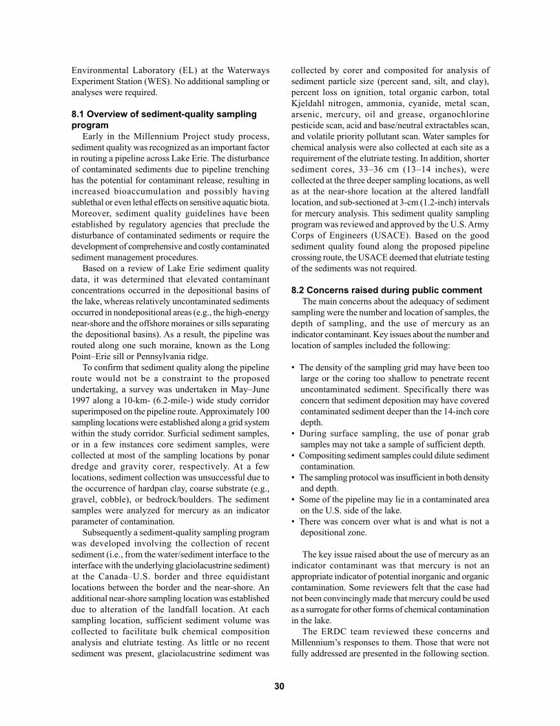
Environmental Laboratory (EL) at the WaterwaysExperiment Station (WES). No additional sampling oranalyses were required.

8.1 Overview of sediment-quality samplingprogram

Early in the Millennium Project study process,sediment quality was recognized as an important factorin routing a pipeline across Lake Erie. The disturbanceof contaminated sediments due to pipeline trenchinghas the potential for contaminant release, resulting inincreased bioaccumulation and possibly havingsublethal or even lethal effects on sensitive aquatic biota.Moreover, sediment quality guidelines have beenestablished by regulatory agencies that preclude thedisturbance of contaminated sediments or require thedevelopment of comprehensive and costly contaminatedsediment management procedures.

Based on a review of Lake Erie sediment qualitydata, it was determined that elevated contaminantconcentrations occurred in the depositional basins ofthe lake, whereas relatively uncontaminated sedimentsoccurred in nondepositional areas (e.g., the high-energynear-shore and the offshore moraines or sills separatingthe depositional basins). As a result, the pipeline wasrouted along one such moraine, known as the LongPoint–Erie sill or Pennsylvania ridge.

To confirm that sediment quality along the pipelineroute would not be a constraint to the proposedundertaking, a survey was undertaken in May–June1997 along a 10-km- (6.2-mile-) wide study corridorsuperimposed on the pipeline route. Approximately 100sampling locations were established along a grid systemwithin the study corridor. Surficial sediment samples,or in a few instances core sediment samples, werecollected at most of the sampling locations by ponardredge and gravity corer, respectively. At a fewlocations, sediment collection was unsuccessful due tothe occurrence of hardpan clay, coarse substrate (e.g.,gravel, cobble), or bedrock/boulders. The sedimentsamples were analyzed for mercury as an indicatorparameter of contamination.

Subsequently a sediment-quality sampling programwas developed involving the collection of recentsediment (i.e., from the water/sediment interface to theinterface with the underlying glaciolacustrine sediment)at the Canada–U.S. border and three equidistantlocations between the border and the near-shore. Anadditional near-shore sampling location was establisheddue to alteration of the landfall location. At eachsampling location, sufficient sediment volume wascollected to facilitate bulk chemical compositionanalysis and elutriate testing. As little or no recentsediment was present, glaciolacustrine sediment was

collected by corer and composited for analysis ofsediment particle size (percent sand, silt, and clay),percent loss on ignition, total organic carbon, totalKjeldahl nitrogen, ammonia, cyanide, metal scan,arsenic, mercury, oil and grease, organochlorinepesticide scan, acid and base/neutral extractables scan,and volatile priority pollutant scan. Water samples forchemical analysis were also collected at each site as arequirement of the elutriate testing. In addition, shortersediment cores, 33–36 cm (13–14 inches), werecollected at the three deeper sampling locations, as wellas at the near-shore location at the altered landfalllocation, and sub-sectioned at 3-cm (1.2-inch) intervalsfor mercury analysis. This sediment quality samplingprogram was reviewed and approved by the U.S. ArmyCorps of Engineers (USACE). Based on the goodsediment quality found along the proposed pipelinecrossing route, the USACE deemed that elutriate testingof the sediments was not required.

8.2 Concerns raised during public commentThe main concerns about the adequacy of sediment

sampling were the number and location of samples, thedepth of sampling, and the use of mercury as anindicator contaminant. Key issues about the number andlocation of samples included the following:

• The density of the sampling grid may have been toolarge or the coring too shallow to penetrate recentuncontaminated sediment. Specifically there wasconcern that sediment deposition may have coveredcontaminated sediment deeper than the 14-inch coredepth.

• During surface sampling, the use of ponar grabsamples may not take a sample of sufficient depth.

• Compositing sediment samples could dilute sedimentcontamination.

• The sampling protocol was insufficient in both densityand depth.

• Some of the pipeline may lie in a contaminated areaon the U.S. side of the lake.

• There was concern over what is and what is not adepositional zone.

The key issue raised about the use of mercury as anindicator contaminant was that mercury is not anappropriate indicator of potential inorganic and organiccontamination. Some reviewers felt that the case hadnot been convincingly made that mercury could be usedas a surrogate for other forms of chemical contaminationin the lake.

The ERDC team reviewed these concerns andMillennium’s responses to them. Those that were notfully addressed are presented in the following section.

30

8.3 Concerns addressed during ERDC reviewThe main premise of the sediment sampling

conducted along the proposed pipeline route is that theroute crosses through the nondepositional Long Point–Erie sill for its entire length, generally avoiding areascharacterized by more heavily contaminated sediments.Many of the concerns that the EL researcher had uponreading the report entitled “Comprehensive StudyReport: Environmental Impact Assessment of theProposed Millennium Project Lake Erie Crossing”(Fitchko 1999) echoed those raised during public reviewby Andrew Martin (1999). These concerns weregenerally addressed in Millennium’s response to DataRequest No. 10 dated August 6, 1999. However, becausethe sediment sampling plan and interpretation ofsediment contaminant results depend heavily on thesupposition that the pipeline route crosses anondepositional area, a number of points neededclarification and expansion. The specific questionsfrom EL are in italics, followed by the response fromBII.

1. What are the reasons for expecting that sedimentmetal concentrations in Lake Erie will co-vary? Discussin relation to contaminant input, contaminant sources,mixing, and deposition patterns. Two correlationcoefficients are reported in the response to data requestNo. 10 between Hg and Cd. It is also stated thatcorrelations existed between Hg and other metals andorganics. These correlations should be shown in a tablefor either discrete data sets or pooled historical data.

With the validity of the entire sediment sampling strategyresting upon the relationships between contaminants,such data presentations would assist evaluation of theuse of Hg as a tracer contaminant.

BII: Metal pollution in Lake Erie is derived from a widevariety of sources, including tributary inputs, shorelineerosion, industrial and domestic effluent discharges, andatmospheric fallout. The atmosphere is now widelyrecognized as a major source of metal pollution incoastal, marine, and lacustrine environments. There isreasonable agreement in reported atmospheric loadingsof metals to Lake Erie (Nriagu et al. 1979). Estimatedsources and sinks of metals in Lake Erie are listed inTable 8.1.

The data in Table 8.1 indicate that a large fraction(approximately 60% for copper and zinc, and 30% forlead) of the total metal burden of the lake is contributedby the Detroit River. Direct atmospheric inputs accountfor 8%, 34%, and 13% of the copper, lead, and zinc,respectively, delivered annually to the lake, whereasthe annual contributions of copper, lead, and zinc fromsewage effluents are 18%, 15%, and 11%, respectively.

The dispersion pathways of anthropogenic metalsand organic contaminants in the Great Lakes are poorlyunderstood.* Substances that enter the lake are subjectedto physical transportation processes and may be

Table 8.1. Sources and sinks of metals in Lake Erie.*

Flux rate (x103 kg/y)

Source Cadmium Copper Lead Zinc

Detroit River (import from — 1,640 630 5,220

Upper Lakes)

Tributaries (U.S.) — 100 52 271

Tributaries (Ontario) — 31 19 140

Shoreline erosion 7.9 190 221 308

Sewage discharges 5.5 448 283 739

Atmospheric inputs 39 206 645 903

Dredged material 4.2 42 56 375

TOTAL (all sources) 2,477 1,906 7,776

EXPORT Niagara River and 1,320 660 4,400

Welland Canal

Retained in sediments 1,157 1,246 3,376

*Source: Nriagu et al. (1979).

31

*Personal communication, A. Mudroch, AMU Ecosystems,2000.

dispersed over wide areas before being transferred outof the water mass into the sediments. Anthropogenicinputs to the lake sediments are greatest in areas withhighest sedimentation rates and are not dependent onproximity to the source areas (Kemp and Thomas 1976).The high sedimentation rates in the eastern basin ofLake Erie are presumably a function of the easterlylocation of the basin in the lake. The prevailing westerlywinds and the west-to-east flow of the Great Lakessystem towards the Atlantic Ocean enables the mosteasterly basins to act as sinks for the fine-grainedsuspended material. In addition, surface fine-grainedsediments in the shallow western basin of Lake Erieare continuously resuspended and transported into thecentral and eastern basins of the lake.

The binding sites for inorganic contaminants (suchas metals) and organic contaminants (such as PCBs) inthe sediments are the hydroxyl groups of the naturaliron and manganese oxyhydroxides and the coatings oforganic matter on these oxyhydroxides (Tessier et al.1996). Fine-grained clay materials in the sediments actas a matrix for the deposition of the oxyhydroxides andthe organic matter (Jenne 1977). Because of thesebinding processes and the fact that the fine-grainedmaterials settle in the depositional basins of lakes, thehighest concentrations of the inorganic and organiccontaminants occur in the sediments of depositionalbasins. This is supported by the relationship among thecontaminants, organic carbon and fine-grained sedimentsfound in different studies of lake sediments (e.g., Thomasand Jaquet 1976). The relationship between metals, PCBs,and organic carbon in sediments collected from Lake Erieduring the 1970s survey undertaken by EnvironmentCanada is shown in Table 8.2.

A relationship was also determined for the metals in

the composite sediment core samples collected alongthe proposed Millennium Lake Erie Crossing route(Table 8.3). However, there was no relationship betweenthe metals and organic carbon in the composite cores,which indicates a different binding mechanism betweenthe sediment particles and the metals than that found inthe sediments in depositional basins. This lack of arelationship between metals and organic carbon likelyreflects the nondepositional nature of the sedimentsalong the proposed pipeline route. The concentrationsof the metals in the composite cores were similar tothose in the precolonial sediments (Table 8.4) in whichthe origin of the metals is, most likely, from naturalmaterials in the lake’s drainage basin.

As indicated in Tables 8.2 and 8.3, there is asignificant (p <0.05) positive relationship betweenmercury and the other metals and PCBs in thesediments. Based on these relationships, the use ofmercury as a tracer contaminant is technically valid.

2. What was the sediment deposition rate (or rates)used in determining the depth of the cores taken alongthe proposed pipeline route? Fitchko (1999) presents asummary of the literature on sources of sediment andsediment deposition rates in Lake Erie, but the sedi-ment deposition rate used in computing the depth ofcores was not given. Explain why the deposition ratesused in determining the depth of cores were conserva-tive and why they should remain constant along theentire pipeline route if that was indeed the assumption?

BII: Sedimentation rates in Lake Erie were presentedin Figure 23 of the Fitchko (1999) report based on astudy undertaken by Kemp et al. (1977). The dataindicate that, in the eastern basin of Lake Erie,

Table 8.2. Correlation of metals, PCBs, and organic carbon in Lake Erie sediments.1

Cd Cr Cu Pb Hg Ni Zn PCBs Org. C2

Cd 1

Cr 0.984 1

Cu 0.886 0.811 1

Pb 0.993 0.967 0.896 1

Hg 0.954 0.959 0.762 0.954 1

Ni 0.934 0.885 0.840 0.962 0.933 1

Zn 0.951 0.906 0.871 0.970 0.899 0.977 1

PCBs 0.943 0.971 0.794 0.918 0.894 0.811 0.866 1

Org. C 0.903 0.849 0.897 0.938 0.824 0.926 0.957 0.815 1

1 Source: A. Mudroch, AMU Ecosystems, 2000, pers. comm.2 Org. C: Total organic carbon.

32

sedimentation rates are greatest in the deep waters southand east of Long Point and appear to decrease towardsthe periphery of the basin toward the north, south, andeast. The highest sedimentation rates are generally foundwhere the thickness of the fine-grained sediment isgreatest, whereas the lowest rates occur where thethickness of fine-grained sediment is the least (Kempet al. 1977). Table 8.5 presents sedimentation rates inthe eastern basin of Lake Erie determined by Kemp etal. (1977). These data indicate that sedimentation ratesin the area of the proposed pipeline route will rangefrom 0 to 1.2 mm/y. Based on these rates, the depth ofrecent sediment (i.e., since 1890) in the area of thepipeline route will range from 0 to 12 cm.

The cores collected for mercury analysis along theproposed pipeline route ranged from 27 to 36 cm indepth (depending upon corer penetration). This depthof sediment core collection is conservative since it wasbased on the findings of Azcue et al. (1996), whoreported that sediment cores collected from adepositional area of the central basin had maximummetal concentrations at about the 18-cm depth and pre-industrial metal levels at about the 36-cm depth (seeTable 4.21 in Fitchko [1999]).

Concentration profiles of Pb210 obtained in the studyof sedimentation rates by Robbins et al. (1978) indicateduniform rates of sediment deposition in Lake Erie andLake Ontario over about the past 100 years or so.Generally consistent rates of sedimentation were alsoobtained from analysis of Cs137 concentration profilesin cores collected in Lake Erie and Lake Ontario by thesame authors. Considering these findings, it can beexpected that the deposition (i.e., sedimentation) rateswill generally remain constant along the entire pipelineroute.

3. The documents reviewed present a somewhatconfusing picture of recent sediment deposition on theLong Point–Erie sill. Page 4:34 of Fitchko (1999) statesthat there was little evidence of deposition of recentsediments along the study corridor, although slightlyanaerobic sediments occurred just offshore on the U.S.

Table 8.3. Correlation of metals and organic carbon in composite sediment core samples col-lected along the Millennium Lake Erie Crossing route.1

Cd Hg Cr Cu Pb Ni Zn Org. C2

Cd 1

Hg 0.995 1

Cr 0.828 0.841 1

Cu 0.943 0.953 0.819 1

Pb 0.638 0.630 0.800 0.501 1

Ni 0.604 0.607 0.842 0.491 0.971 1

Zn 0.858 0.851 0.875 0.728 0.935 0.905 1

Org. C 0.244 0.271 0.241 0.329 –0.102 0.013 0.090 1

1 Source: A. Mudroch, AMU Ecosystems, 2000, pers. comm.2 Org. C: Total organic carbon.

Table 8.4. Mean concentrations of metals inprecolonial sediments and in the compositesediment cores collected along the proposedpipeline route.1

Concentration (µg/g)

CompositeMetal Precolonial sediment cores

Arsenic 3.7 3.412

Cadmium 0.37 0.30Chromium 35 17.5Copper 29 13.9Lead 15 13.9Mercury 0.078 0.075Nickel 48 16.9Zinc 98 40

1

Source: A. Mudroch, AMU Ecosystems, 2000, pers.

comm.2 Value for station CS8 was not included in the calcula-tion of the mean value for arsenic. As indicated in Fitchko(1999), the elevated level of arsenic at this samplinglocation was likely due to natural post-depositional mi-gration of arsenic in the sediment pore water and sub-sequent oxidation of arsenate at the sediment surfacewith adsorption and concentration particularly onto man-ganese oxyhydroxides. If the value for this station isincluded, the mean value for arsenic would be 5.9 µg/g.

33

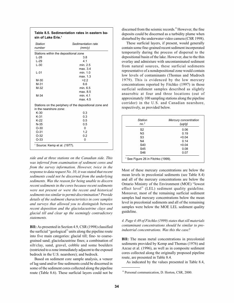
side and at three stations on the Canadian side. Thiswas inferred from examination of sediment cores andfrom the survey information. However, twice in theresponse to data request No. 10, it was stated that recentsediments could not be discerned from the underlyingsediments. Was the reason for being unable to discernrecent sediments in the cores because recent sedimentswere not present or were the recent and historicalsediments too similar to permit discrimination? Providedetails of the sediment characteristics in core samplesand surveys that allowed you to distinguish betweenrecent deposition and the glaciolacustrine clays andglacial till and clear up the seemingly contradictorystatements.

BII: As presented in Section 4.9, CSR (1998) classifiedthe surficial “geological” units along the pipeline routeinto five main categories: glacial till; fine- to coarse-grained sand; glaciolacustrine fines; a combination ofsilt/clay, sand, gravel, cobble and some boulders(restricted to a zone immediately adjacent to the exposedbedrock in the U.S. nearshore); and bedrock.

Based on sediment core sample analysis, a veneerof lag sand and/or fine sediments could be discerned insome of the sediment cores collected along the pipelineroute (Table 8.6). These surficial layers could not be

Table 8.5. Sedimentation rates in eastern ba-sin of Lake Erie.1

Station Sedimentation ratenumber (mm/y)

Stations within the depositional zoneL-28 3.8L-29 4.1L-30 min. 2.5

max. 3.4L-31 min. 1.0

max. 1.3M-30 >2.2M-31 6.6M-32 min. 6.5

max. 8.5M-34 min. 4.1

max. 4.5

Stations on the periphery of the depositional zone andin the nearshore zone:K-30 0.3K-31 0.3K-22 0.5N-35 0.5O-30 0O-31 1.2O-32 0.2O-33 0

1 Source: Kemp et al. (1977).

discerned from the seismic records.* However, the finedeposits could be discerned as a turbidity plume whendisturbed by the underwater video camera (CSR 1998).

These surficial layers, if present, would generallycontain some fine-grained recent sediment incorporatedtemporarily during the process of dispersal to thedepositional basin of the lake. However, due to the thinoverlay and admixture with uncontaminated sedimentfrom natural sources, these surficial sedimentsrepresentative of a nondepositional zone would containlow levels of contaminants (Thomas and Mudroch1979). This is evidenced by the low mercuryconcentrations reported by Fitchko (1997) in thosesurficial sediment samples described as slightlyanaerobic at four and three locations (out ofapproximately 100 sampling stations along the pipelinecorridor) in the U.S. and Canadian nearshore,respectively, as provided below.

Station Mercury concentrationno.1 (µg/g)

S2 0.06N3 0.19S3 <0.04N4 0.14S40 <0.04S45 0.08S46 0.07

1 See Figure 26 in Fitchko (1999).

Most of these mercury concentrations are below themean levels in precolonial sediments (see Table 8.4)and all of the mercury concentrations are below theOntario Ministry of the Environment (MOE) “lowesteffect level” (LEL) sediment quality guideline.Moreover, most of the remaining surficial sedimentsamples had mercury concentrations below the meanlevel in precolonial sediments and all of the remainingsamples were below the MOE LEL sediment qualityguideline.

4. Page 4:49 of Fitchko (1999) states that sill materialscontaminant concentrations should be similar to pre-industrial concentrations. Was this the case?

BII: The mean metal concentrations in precolonialsediments provided by Kemp and Thomas (1976) andAzcue et al. (1996), as well as in composite sedimentcores collected along the originally proposed pipelineroute, are presented in Table 8.4.

As indicated by the values presented in Table 8.4,

34

* Personal communication, D. Horton, CSR, 2000.

the mean concentrations of the metals in the compositesediment cores are lower than those in Lake Erieprecolonial sediments.

5. In the sediment sampling plan the assumption wasthat sediment resuspension and reworking wereconstant. Therefore surface concentrations should berepresentative of deeper contaminant concentrations.Was this shown to be a correct assumption for thesampling program?

BII: Based on the responses to the previous fourWES concerns, the assumption that the surfacecontaminant concentrations are representative ofdeeper concentrations is technically valid. Thisassumption has been confirmed by the determinationthat mercury concentrations in sediment cores col-lected along the pipeline route and subsampled at3-cm intervals were all below the analytical detectionlimit and the mean mercury concentration in pre-colonialsediments (see Tables 4.22 and 4.25 in Fitchko [1999]).

8.4 Status of concernsThe BII responses to the EL concerns regarding the

sediment sampling and analysis program answered thequestions raised. A major concern was the utility of

mercury as a tracer contaminant. Based on the relativelylimited major sources of contamination to the lake, wefelt that there was an excellent chance that correlationsbetween mercury and other contaminants should exist.However, this had not been demonstrated in eitherFERC (1999) or the supporting material. Our concernson this issue were answered by the strong correlationsbetween mercury and other contaminants in twoindependent data sets, including the sediment corescollected for the Millennium Project.

Another major concern was the depth of sedimentcores and the depositional environment along thepipeline route. Depth of sediment sampling is a complexissue and depends to a great extent on the depositionalenvironment of the pipeline route. Detailed examinationof the geophysical survey results in conjunction withthe clarifications on sediment deposition rates andphysical observations of core stratigraphy indicate thatthe deposition rates used for determining core sampledepths were conservative and should encompasshistorical contamination, if present. Compositing a coreto obtain an overall value is an acceptable procedure.Resuspension of the material during trenchingoperations will mix the entire core depth in the watercolumn. Therefore, the composite is representative ofreal-world exposures.

Table 8.6. Surficial sediment core sample logs.1

Location2 Sediment depth (cm) Sediment description

1A 0–5 Clay, very soft, occasional small shells, gravelly, gray.>5 Clay, firm, organic lenses, light brown.

1B3 0–37 Alternating dark gray-brown and dark gray layers; appears to bemostly fine sand; some mussel shells at surface.

2 Surface Clay, soft, shells (mussels), dark gray.Below surface Clay, very soft, dark gray, minor organic lenses, occasional pebbles.

3 0–2 Sand, loose, fine with shells overlying clay, soft, tan (oxidized layerat base of sand).

>2 Clay, soft, organic lenses, gray.4 0–4 Sand, fine, loose, clay, soft, sandy, tan.

>4 Clay, soft, sandy, graywith numerous organic layers.

5 Surface Clay, very stiff, gravel (pebbles) and numerous mussels at lakebed.Below surface Clay, stiff to very stiff, brown, gravel on top.

6 0–15 Clay, very soft, sandy, gray, occasional mussels at lakebed.15–16 Clay, stiff, light brown.>16 Clay, very soft, sandy gray.

7 0–1 Veneer of sand, gravel, shells, numerous small mussels and soft clay.>1 Clay, stiff, light brown.

8 0–1 Veneer of clay, sandy, gravelly, shelly, numerous mussels.>1 Clay, very stiff.

9 Surface Clay, soft, minor sand, abundant organic material, gray.Below surface Clay, gray, soft, sandy, abundant organic material, layered.

1 Source: Racal Pelagos (1997).2 See Figure 27 in Fitchko (1999).3 Source: CSR (1998).

35

The data in FERC (1999) and supportingdocumentation show that concentrations of mercury andother metals in the sediments along the pipeline routeare relatively low. The comparison to precolonialsediment levels in the response clarified the datapresentation and put present-day sediment metalconcentrations into better perspective.

Therefore, all sediment-sampling issues examinedduring the ERDC review were addressed satisfactorily.This conclusion holds true for the ~20% deeper trenchdepths required in zones H–J (Chapter 6) due to therevised 100-year ice scour depths. The additionalmaterial excavated would be uncontaminated sedimentand thus would not increase environmental exposuresto contaminated sediments.

9.0 TURBIDITY MODELING

BEAK International, Inc. (BII) acted on behalf ofthe Millennium Project to model turbidity generationand sediment deposition arising during constructionof the Lake Erie crossing. Concerns raised duringpublic review of the Millennium Pipeline Project DraftEnvironmental Impact Statement (FERC 1999), andits supporting documents (e.g., Fitchko 1999),focused primarily on the adequacy of the modelingand the sensitivity of the results to pipeline trenchdepth.

This chapter briefly describes the turbidity modelingand presents the ERDC review of it. Most issues wereresolved through a question–answer exchange betweenBII and Dr. Mark Dortch of the ERDC EnvironmentalLaboratory (EL) at the Waterways Experiment Station(WES) (Section 9.2). Dr. Paul Schroeder at ELconducted his own analyses with a different model toquantify the effects of model simplifications made byBII (Section 9.3). However, BII was not required toconduct additional analyses.

9.1 Overview of turbidity modelingTurbidity generation and siltation from pipeline

trenching and directional drilling for the MillenniumLake Erie crossing were identified as potentially havinga significant ecological and aesthetic impact. Turbiditymodeling was undertaken to predict

• The concentration, physical extent, and duration ofthe suspended solids plume produced by the operationof a jet sled during pipeline trenching.

• The potential increase in sediment layer thickness oneither side of the trench.

• The concentration, physical extent, and duration ofthe suspended solids plume caused by loss of drilling

mud from the directional drilling operation.

The initial modeling of the suspended-sedimentplume produced by the jet sled operation was based onthe following assumptions:

rate of travel ............................. 0.017 m/s (200 ft/h)trench depth ............................. 2.6 m (8.5 ft)trench width ............................. 4.0 m (13 ft)nozzle diameter ........................ 25 cm (10 inches)nozzle height ............................ 3 m (10 ft)nozzle offset ............................. 2 m (6 ft)nozzle angle ............................. 45 degrees above

horizontalhours of operation .................... continuousdischarge velocity .................... 1–5 m/s (3–16 ft/s)discharge concentration ........... 10–200 g/Lmin. depth of operation ........... 9 m (30 ft).

It was assumed that the jet sled has two dischargeports (one on each side), with sediment being dischargedequally on each side, and that the operation is completedin two passes. Although two passes would be requiredfor trenching, the turbidity plume modeling predictionswere conservatively based on the discharge of the entirevolume of sediments in the trench. Under someconditions a suction hose may be used to removesediment from the trench and discharge it at the surfacefrom the barge at 18 m (59 ft) forward and 14 m (46 ft)off center. The flow rate of the suction pump wasestimated to be 0.8 m3/s (18,500 gpm).

With regard to the conditions in Lake Erie, it wasassumed that the sediment particle density was 2.65 g/cm3. Analyses of the sediments along the proposedpipeline corridor indicate that the sediment isapproximately 75% solids by mass. The sediment solidsdensity was estimated to be approximately 1.39 g/cm3.The following assumptions were also made:

water temperature ......................... 15°C (59°F)ambient average ............................ 0–0.05 m/s

hypolimnion current (0–0.16 ft/s)ambient average ............................ 0.03–0.18 m/s

epilimnion current (0.1–0.6 ft/s).

A second modeling iteration for the jet sled dischargewas undertaken based on a minimum depth of operationof 7.6 m (25 ft).

A third modeling iteration for the jet sled dischargewas undertaken based on the following revisedassumptions:

rate of travel ............................. 0.042 m/s (500 ft/h)trench depth ............................. 2.0 or 2.8 m (6.6 or

36

9.2 ft) depending onroute section

trench width (top) .................... 8.0, 10.4, or 11.8 m(26, 34, or 39 ft)depending on routesection

trench width (bottom) .............. 2.4 m (7.9 ft)trench cross section ................. 12.8, 14.6, or 19.8 m2

(138, 157, or 213 ft2)depending on routesection

nozzle diameter ........................ 40.6 cm (16 inches)nozzle height ............................ 3–4.6 m (10–15 ft)nozzle offset ............................. 2–3 m (6–10 ft)nozzle angle ............................. 45° above horizontalhours of operation .................... continuousdischarge velocity .................... 1.5–3 m/s

(4.9–10 ft/s)discharge concentration ........... 10–200 g/Lmin. depth of operation ........... 11.7 m (38 ft).

It was again assumed that the jet sled has two dischargeports (one on each side), with sediment being dischargedequally on each side. However, the jet sled operationmay require multiple passes to achieve therecommended trench depths. For modeling purposes, aconservative assumption was made that the entirevolume of sediment from the trench would be removedwith only two passes (each pass removing half of thesediment volume). Should more than two passes berequired, the resulting plumes would be of lesser extentand duration.

Turbidity modeling was also used to predict theimpacts of sediment resuspension as a result of thedirectional drilling. The initial modeling was based onsix stages to the directional drilling, of which only thefirst and last use drilling mud (bentonite mixture),whereas the others use water. The specific gravity ofthe drilling mud ranged from 1.10 to 1.15, whichcorresponds to a suspended solids concentration rangeof approximately 160–240 g/L.

The initial pilot hole was less than 25 mm (10 inches)in diameter and was expected to lose 500 barrels/h(0.022 m3/s) for a total of two hours. During thepullback stage, the hole diameter was 1.2 m (48 inches)and was expected to lose 1300 barrels/h (0.057 m3/s)and take approximately one day.

A second modeling iteration for the directional drilldischarge was undertaken based on drilling mud lossduring all stages of directional drilling. The rate ofbentonite loss increases with the hole diameter. Thelowest rate of 10 barrels per minute (1.6 m3/min) startsafter the pilot hole is completed. The largest rate of 20barrels per minute (3.2 m3/min) occurs during the final

reaming process just prior to the final pipe pullback.The specific gravity of the drilling mud (bentonite) wasassumed to be 1.15, which corresponds to a suspendedsolids concentration of 240 g/L. Under calm conditions(unmixed), the along-shore current was assumed to be0.1 m/s (0.32 ft/s), whereas under storm conditions(mixed), the along-shore current was assumed to be 0.2m/s (0.65 ft/s).

The modeling approach was divided into foursections:

• Dense Plume Model. This model component was usedto predict the jet trajectory from the nozzle to thelake bed (modeled by CORMIX1).

• Settling Model. This model component was used topredict the distribution of the disturbed sediments inthe areas adjacent to the pipeline trench.

• Visible Plume Model. This model component wasused to predict the extent and duration of the turbidityplume caused by the jet sled operation and directionaldrilling.

• Dense Turbidity Plume. This model component wasused to determine the behavior of a dense turbidityplume along the lake bottom as a result of directionaldrilling under calm conditions.

The turbidity plume modeling was based onmaximum plume dimensions (length and width) for totalsuspended solids concentrations of 35, 1,000, and10,000 mg/L.

9.2 Concerns addressed during the ERDCreview

This section contains the question–answer exchangebetween EL and BII. These are grouped according tothe Millennium documents cited. The specific ELquestions are in italics, followed by the response fromBII. In a few cases, the cycle repeats.

9.2.1 General observation regarding EL reviewcomments

The intent of the turbidity plume modeling was toprovide an estimate of the extent of the impactassociated with the operation of the jet sled during LakeErie Crossing pipeline trenching operations. Theapproach used was technically valid and of sufficientrigor to scope the issues of concern as part of theenvironmental impact assessment process. TheCORMIX model used is an expert system developedby Cornell University to predict the mixingcharacteristics of a discharge into a natural water body.The model is widely used and accepted by variousregulatory agencies in Canada and the United States.Moreover, the conservative nature of the assumptions

37

used in this modeling study resulted in an overestimateof the extent of the impacts. The use of a more detailedmodeling approach would likely provide impactestimates that are smaller than the estimates provided.Additionally, a detailed modeling study would requirea more significant effort in terms of time and resourcesand would have a more intense data requirement thanis currently available. Since the results of the turbidityplume modeling have been deemed environmentallyacceptable by the state regulatory agencies, it is opinedthat any additional, more detailed modeling isunnecessary at this time.

9.2.2 Comprehensive Study Report (Fitchko 1999),main text

Page 5.32. It is stated that the maximum plumearea will be 28,000 m2 for TSS = 1000 mg/L and forthe Canadian near-shore. However, data in Appendix3 indicate the area will be nearly twice as large, or48,000 m2. There are other similar understatedinconsistencies.

BII: If the plume is assumed to be rectangular, thencalculating the area by multiplying the length by thewidth would be appropriate (i.e., 300 m × 160 m =48,000 m2). However, the plume is a shape similar toan ellipse that is larger at one end. The area of this shapeis approximately 60% of the area calculated using the“rectangular” assumption.

9.2.3 Comprehensive Study Report (Fitchko 1999),Appendix 3

1. General: It surely would have been helpful if theauthors had presented a figure to schematize each ofthe four types of modeling approaches employed (i.e.,dense plume, settling model, visible plume, and denseturbidity plume), showing orientation and featuresrelative to the trench, variable definitions relative tothese features, etc. The lack of figures almost gives theimpression of trying to make this as difficult to followas possible.

BII: Figures depicting the orientation and other featuresof the plume were not provided in our report as thedesign specifications for the jetting operations have notbeen finalized. As stated above, the analysis wasintended to scope the issues of concern and identifyareas where more information is required. Wheninformation was missing, assumptions were made thatwould err on the conservative side. Given this approach,the results should be viewed as worst case. Since acomprehensive monitoring program will beimplemented during construction, an exhaustiveanalysis of turbidity predictions is not required.

Moreover, as indicated in the Monitoring Plan requestedand accepted by the Pennsylvania Department ofEnvironmental Protection (PaDEP), a “footprint” of thevisible plume with appropriate TSS concentrationisopleths (e.g., 10,000 mg/L, 1,000 mg/L, 500 mg/L,and 35 mg/L) will be modeled and plotted foreach zone. These modeling predictions will be basedon final design specifications and used to establish thesampling grid that will overlap the predicted plume ineach zone.

2. Page A3.3. There is not nearly enough informationpresented to evaluate the application of the CORMIX1model for the dense jet. As a minimum, the followingshould be supplied:

a. model assumptions and limitations;

BII: As indicated above, CORMIX is generallyaccepted as a plume model in both Canada and theUnited States. If a detailed modeling study werenecessary, then a complete listing of assumptions andlimitations of CORMIX would be appropriate.However, as a screening tool and to conservativelypredict construction-related impacts, a complete listingof the assumptions and limitations of CORMIX wasnot required.

b. why this model option was selected over the otherCORMIX package modeling options, i.e., how or inwhat way the jet sled discharge fits this model and itsassumptions;

BII: CORMIX1 refers to the single-port dischargemodel included in the CORMIX package. The othercomponents (i.e., multi-port and surface discharges) arenot appropriate to examine the behavior of the plumeas it exits the jet sled.

c. a list of model input variables and values used;

BII: This information was provided on page A3.1.

d. a list of model parameters (e.g., coefficients), valuesused, and justification for their use;

BII: The coefficients used in CORMIX are notchangeable (i.e., they are hard-wired into the program).In previous projects, BEAK has examined the sourcecode for CORMIX and determined that it is consistentwith jet theory presented in the literature. Thecoefficients used are generally biased toward aconservative estimate (i.e., predicts a longer plume withlower dilution).

38

e. any attempt to validate the model for this use, andthose results.

BII: There were no attempts to validate the predictionsof CORMIX since the data are not available. However,at the request of the PaDEP, a detailed monitoring planhas been developed and accepted to confirm the resultsof the turbidity plume modeling.

Additionally, since this jet will contain highconcentrations of sediment, there will be a negativelybuoyant jet-plume effect that should have been takeninto consideration. There is no mention of this effect orthe input of data to describe the density differencebetween the jet and ambient water. If TSS concentrationof the jet was used to determine the density of the jeteffluent, then what formula was used to compute jetfluid density from TSS concentration data?

BII: The discharge from the jet sled will likely producea dense bottom plume as indicated by CORMIX. Theplume is expected to be 0.5–2 m thick once it contactsthe bottom. The density of the jet discharge was basedon an ambient water temperature of 15°C and asuspended sediment concentration of 30–200 g/L. Thedensity difference was calculated using

∆ ρ = 0.00062 * TSS.

This relationship is used in the CE-QUAL-W2 modeldeveloped by the Corps of Engineers. The resultingdensity difference ranges from 17 to 123 kg/m3.

3. Page A3.3. What value of Z was used in Equation1, the mid-height of the plume or the top of the plume?The top of the plume makes more sense, but it is notclear what was used.

BII: The distance from the lake bottom to the top ofthe dense plume was used and is represented as Z.

4. Page A3.4. Is S the cross-sectional area of thetrench? If yes, then Equation 3 makes sense, otherwiseit does not. The definition of S should be stated moreprecisely. Equation 3 assumes that the redepositedsediment will have the same porosity as the undisturbedsediment in the trench, thus there is no effect ofunconsolidation during removal of the consolidatedsediments in the trench. The redeposited sediment willlikely have a greater porosity, will be less consolidated,and thus have a greater thickness than predicted byEquation 3. Given the expected porosity, or bulk density,of the redeposited sediment and the porosity, or bulkdensity, of the trench sediment prior to removal, it should

be possible to more accurately estimate the redepositedsediment thickness.

BII: Yes, S represents the cross-sectional area of thetrench. Since there were no data available regardingthe variation of porosity with depth or the porosity offreshly deposited sediment, it was reasonable to assumethe same porosity. While the initial deposits ofsediments may be somewhat thicker than predicted,these unconsolidated sediments will be subject totransport by wave and current action. A portion of thesesediments will eventually redeposit in the trench. Thesediment remaining in the deposit areas will eventuallyconsolidate to a porosity similar to the undisturbedsediment. Additionally, a fraction of the sediment willremain within the trench during the operation of the jetsled and will not contribute to the deposit thickness orthe turbidity plume. This fraction is highly variable and,in order to be conservative, was ignored.

EL response: To ignore bulking is to underestimate thedepth of burial of environmental resources and thereforenonconservative. Reasonable guesses of porosity as afunction of time can be made from settling andconsolidation data bases for dredged material.

BII: BEAK concurs that disregard of sediment bulkingas a variable affecting redeposited sediment thicknesswill result in an underestimate of the depth of burial ofenvironmental resources. As indicated in the EA Report(Fitchko 1999), the magnitude of the impacts on thebenthic community will be a function of several factors:the duration and volume of trench excavation; relativesurvival rate of the species dependent primarily on theircapacity for drifting or moving away from thedisturbance; relative species survival rates dependentprimarily on their capacity to move through any spoilmounds formed adjacent to the trench and thus avoidcrushing or smothering; and relative speciesrecolonization rates after natural backfilling. Althoughthe predicted depth of burial will likely be greater takinginto account sediment bulking and may result in greaterreductions in biomass, species number, and populationsize of the benthic biota, recolonization is expected tobe rapid and the impact will be localized and temporary.

5. Page A3.4. It is stated that 10% to 45% of theparticles did not settle in the analysis. I don’t followthis statement. Does this mean that the finer size classesof sediment required such long distances to settle thattheir results were off the graph, or what? All particlesshould settle eventually. The statement is made earlieron Page A3.4 that the total sediment thickness at anypoint is calculated as the sum of all the individual

39

thicknesses that have a distributed distance equal to orgreater than the distance at that point. Therefore, itseems that all particle size classes should be includedin the calculation of the redeposited sedimentthicknesses, thus all particles settle somewhere. TheCorps of Engineers experiences have been that about97% of dredged material disposed in aqueousenvironments impacts the bottom near the vicinity ofdischarge, and the rest remains in suspension muchlonger. The 10 to 45% statement does not seemconsistent with this result.

BII: In the particle size distributions provided by GAIConsultants Inc., a fraction of the particles were smallerthan 0.001 mm and were not accounted for. Theseparticles would contribute to the deposit thickness, butsince they have a very small settling velocity, they wouldbe spread out over a large distance and contribute avery small increase to the overall deposit thickness. Itwas determined that this minor component would notadd to the overall construction-related impacts withrespect to deposit thickness. However, this fine fractionwas taken into account in turbidity modeling.

6. Page A3.4. At the bottom of the page, it is statedthat since the suction discharge is located above thewater, it will not form a dense bottom plume. How dothe authors know this will be the case?

If the discharge is placed 3.7 m above the water surface,the energy dissipation (i.e., mixing) of the discharge atthe water surface will initially dilute the plume and inturn decrease the density difference between the plumeand the ambient water. Even if the plume sinks to thebottom, mixing with the ambient water will “spread”the sediment through the water column.

EL response: Discharges above the water surface tendto promote development of density flow because the jetloses most of its horizontal momentum in the air andupon hitting the surface. Discharges into the air understeady conditions actually entrain less ambient waterthan submerged discharges, particularly angleddischarges, because they tend to entrain the dischargedwater rather than jetting through the clean watercolumn at an angle. Additionally, the discharge fromthe suction pump is larger than the ambient flow throughthe cross-sectional area of the discharge plume, yieldinglittle potential for significant dilution under steady-stateoperation. Thus, it is most likely that the plume willsink to the bottom and form a bottom layer of movingsediment (i.e., a bottom density current). As Dr.Schroeder points out in his memo (Section 9.3), the D-CORMIX model could be used to assess this. No further

action on this issue is expected, rather the point is madefor future analyses.

BII: BEAK will take into account the potentialapplicability of the D-CORMIX model to better modelthe dense jet resulting from surface discharge if futureanalyses are required.

7. Table 1. Several additional cases should be run,such as Core 7 with Case 1 conditions and Core 2 withCase 3 conditions. It seems that otherwise, it is notreadily apparent which are the best and worst caseconditions/results. These additional runs would helpbracket outcomes.

BII: As indicated in the response to PaDEP DeficiencyQuestion 2i, additional modeling has been undertakento predict the turbidity plumes produced by theoperation of a jet sled within five zones along thepipeline route in U.S. waters based on zone-specificrecommended trench depths, average water depths, andsediment particle sizes. These modeling resultssupercede those in Table 1, as they take into accountzone-specific conditions. However, to respond to yourcomment, one extreme case would be if a sediment witha large particle size (i.e., Core 2) is allowed to settleover a smaller vertical distance (i.e., 0.5 m) and is notcarried by an ambient current, i.e., the ambient currentis 0 m/s. This would result in the sediments beingdeposited in a thicker layer over a shorter distance. Theopposite case would be if a fine sediment (i.e., Core 7)is allowed to settle over a longer vertical distance (i.e.,2 m) and is carried by a stronger ambient current. Thiswould result in the sediments being deposited in athinner layer over a longer distance. By reversing someof the cores, the case represented would fall betweenthe two extremes represented above.

8. Page A3.6. What is the basis for the assumptionof when the plume is visible, i.e., Secchi depth equal to1.0 m?

BII: A Secchi depth of 1 m seemed reasonable. TheOntario MOE (1979) had established a water qualitycriterion for Secchi disc transparency of at least 1.2 mfor recreation and aesthetics.

9. Page A3.6. Where does the value of q = 123,000g/s come from? I tried using the jet exit diameter,velocity, and sediment concentration, and did not arriveat this value. A figure earlier may have helped clearthis up for me.

BII: The discharge rate was calculated by multiplying

40

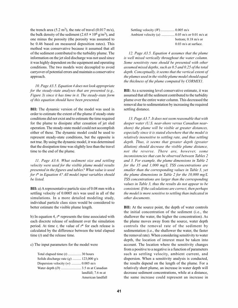
the trench area (5.2 m2), the rate of travel (0.017 m/s),the bulk density of the sediment (2.65 × 106 g/m3), andone minus the porosity (the porosity was assumed tobe 0.46 based on measured deposition rates). Thismethod was conservative because it assumed that allof the sediment contributed to the turbidity plume. Theinformation on the jet sled discharge was not used sinceit was highly dependent on the equipment and operatingconditions. The two models were decoupled to avoidcarryover of potential errors and maintain a conservativeapproach.

10. Page A3.5. Equation 4 does not look appropriatefor the steady-state analyses that are presented (e.g.,Figure 3) since it has time in it. The steady-state formof this equation should have been presented.

BII: The dynamic version of the model was used inorder to estimate the extent of the plume if steady-stateconditions did not exist and to estimate the time requiredfor the plume to dissipate after cessation of jet sledoperation. The steady-state model could not accomplisheither of these. The dynamic model could be used torepresent steady-state conditions, but the opposite isnot true. By using the dynamic model, it was determinedthat the dissipation time was slightly less than the traveltime to the end of the plume.

11. Page A3.6. What sediment size and settlingvelocity were used for the visible plume model resultspresented in the figures and tables? What value is usedfor t* in Equation 4? All model input variables shouldbe listed.

BII: a) A representative particle size of 0.08 mm with asettling velocity of 0.0005 m/s was used in all of thesimulations. In a more detailed modeling study,individual particle class sizes would be considered tobetter estimate the visible plume length.

b) In equation 4, t* represents the time associated witheach discrete release of sediment over the simulationperiod. At time t, the value of t* for each release iscalculated by the difference between the total elapsedtime (t) and the release time.

c) The input parameters for the model were

Total elapsed time (t) ............... 30 hoursSolids discharge rate (q) .......... 123,000 g/sDispersion velocity (w) ........... 0.005 m/sWater depth (D) ....................... 3.5 m at Canadian

landfall; 7.6 m atAmerican landfall

Settling velocity (W) ................ 0.005 m/sAmbient velocity (u) ............... 0.05 m/s or 0.01 m/s at

bottom; 0.18 m/s or0.03 m/s at surface.

12. Page A3.5. Equation 4 assumes that the plumeis well mixed vertically throughout the water column.Some sensitivity runs should be presented with otherassumed mixed depths, such as 0.5 and 0.25 of the totaldepth. Conceptually, it seems that the vertical extent ofthe plumes used in the visible plume model should equalthe thickness of the plume computed by CORMIX1.

BII: As a screening level conservative estimate, it wasassumed that all the sediment contributed to the turbidityplume over the entire water column. This decreased theremoval due to sedimentation by increasing the requiredsettling distance.

13. Page A3.7. It does not seem reasonable that withdeeper water (U.S. near-shore versus Canadian near-shore) the plume will be visible at greater distances,especially since it is stated elsewhere that the model isrelatively insensitive to settling rate, and thus settlingdepth. Thus, it seems that greater depth (greaterdilution) should decrease the visible plume distance,not the reverse. There are, however, someinconsistencies that can be observed between Tables 2and 3. For example, the plume dimensions in Table 2for the 35 and 1,000 mg/L TSS concentrations aresmaller than the corresponding values in Table 3, yetthe plume dimensions in Table 2 for the 10,000 mg/LTSS concentrations are larger than the correspondingvalues in Table 3, thus the results do not appear to beconsistent. If the calculations are correct, then perhapsthe model is more sensitive to settling than indicated inother documents.

BII: At the source point, the depth of water controlsthe initial concentration of the sediment (i.e., theshallower the water, the higher the concentration). Asthe plume moves away from the source, water depthcontrols the removal rate of the sediment bysedimentation (i.e., the shallower the water, the fasterthe removal rate). When considering sensitivity to waterdepth, the location of interest must be taken intoaccount. The location where the sensitivity changesfrom a positive to a negative is a function of parameterssuch as settling velocity, ambient current, anddispersion. When a sensitivity analysis is conducted,the results depend on the length of the plume. For arelatively short plume, an increase in water depth willdecrease sediment concentrations, while at a distance,the same increase could represent an increase in

41

sediment concentrations relative to the base case.

14. Page A3.8. How was the drill mud plumethickness of 0.2 m derived from CORMIX1?

BII: The directional drill hole was represented as asingle port submerged discharge. The exit velocity anddensity were based on estimates provided by thedirectional drilling contractor. The CORMIXpredictions indicated that under calm conditions theflow of drilling mud would form a dense bottom plumeapproximately 0.2 m thick and travel at a speedapproximately equal to the ambient current.

15. Page A3.9. Were equations 1–3 used to calculatethe bentonite accumulation thickness on the bottom of2.4 mm?

BII: The predicted depths are based on a similarapproach as equations 1 through 3 except that only oneparticle size was used. The drilling mud is comprised ofuniform bentonite clay with a particle size of 0.001 mm.

9.2.4 January 28, 2000 letter, supplementalresponse no. 3 to Penn. DEP letter of December3, 1999, question no. 21

1. Page 5. I believe the DO analysis is flawed. A kdvalue on the order of 10–5 day–1 was used. This valueis more representative of the diagenesis of refractivesediment organic matter and is not representative ofthe oxidation rate of reduced sediments and pore waterthat have been taken from an anaerobic environmentand exposed to oxygenated water. Such sediments cancontain reduced iron and manganese, ammonium,sulfide, and possibly methane. When introduced tooxygenated water, much of the reduced matter isoxidized rather rapidly, exerting a rapid chemicaloxygen demand. Our respirometer studies with dredgedsediments indicate COD decay rates on the order of1.5 day–1. Also, equation 4 should be restated from thefirst order COD (or BOD) decay law, or

∆O2 = CTSS COC (1 – e–kd t).

Using kd = 1.5 day–1, CTSS = 10,000 mg/L, COD = 3g/1,000 g sediment (typical value found from dredgedmaterial respirometer studies), and t = 5 hours, theabove equation yields ∆O2 = 8.0 mg/L. In contrast,using the equation shown in the memo (equation 4) withthese values yields ∆O2 = 9.4 mg/L. These values arethe dissolved oxygen (DO) demand that would beexerted in a respirometer or BOD bottle over five hoursgiven a water and dredged material mixture that results

in 10,000 mg/L of sediment. This is not necessarily theDO uptake that would occur wherever the TSSconcentration is 10,000 mg/L in the prototype watercolumn since it is believed that much of the COD isassociated with dissolved reduced constituents releasedfrom the pore water that may not disperse as far as thesolids. However, it is still possible that much greaterDO demand will be exerted than anticipated, especiallyin the near field, highly concentrated TSS region. ThisDO demand will be rapidly diffused and diluted, willbe short lived, and may be exerted in a smaller areathan the 10,000 mg/L TSS contour. If DO is potentiallya concern, then there are methods for measuring CODand kd for dredged material. However, a moresophisticated modeling analysis would need to beemployed so that 3D (or at least 2D) advection,diffusion, COD loading (g/sec), COD decay, and DOuptake can all be taken into account simultaneously. Acopy of a draft paper I have written describesapproaches for measuring and modeling DO uptakeassociated with dredged material disposal. This papercan be furnished to the authors if this is of interest orconcern.

BII: As the turbidity plume moves away from the jetsled, oxygen consumption will decrease with thedecrease in TSS concentration as it mixes with thesurrounding water. While it is true that the COD woulddecay on a first-order relationship, the simple approachdoes exclude mixing of ambient oxygenated water asthe plume spreads, i.e., as the oxygen is consumed bythe suspended sediment, there is a significant amountof oxygen being drawn into the plume from thesurrounding water to offset this consumption. A detailedmonitoring plan has been developed, that has beenaccepted by the PDEP, to monitor potential oxygendepletion in the hypolimnion during trenchingoperations. Please provide us with a copy of your draftreport for our review and confirmation that yourrespirometer results are applicable to the Lake Eriesediments along the proposed pipeline route.

2. Monitoring should include temperature and DOmonitoring within the 10,000 mg/L TSS contour. Thememo did not make this clear.

BII: The monitoring plan requires temperature and DOmeasurements at a minimum of three sampling locationswithin the plume, i.e., near-, mid- and far-field. Theselocations correspond to the 10,000 mg/L, 1,000 mg/L,and 35 mg/L contours. Therefore, temperature and DOmonitoring will occur within the 10,000 mg/L contour,where practicable from a safety standpoint.

42

9.2.5 Millennium pipeline letter of December 27,1999, in response to Penn. DEP letter ofDecember 3, 1999, and in response toOPR/DEER, ERC II memo dated October 1, 1999

1. Section 2i. Was the average particle size andassociated settling velocity used for the visible plumemodel to generate the results that are presented? If so,then the preferred approach would be to apply the plumemodel for each class of sediment size to calculateCi(x,y,t) and add the class concentration values togetherto get the total concentration. It is possible that thevisible plume may extend farther than indicated whenconsidering the smaller sediment sizes. This commentapplies not only to this memo but to all analysesassociated with estimating the visible plume size.

BII: See response to Appendix 3, No. 11a (Section9.2.3).

2. Section 2i table. Please explain why the table insection 2i shows larger plume dimensions than theBEAK report for Zone F and for the 35 and 1,000 mg/L TSS concentrations, but it shows smaller dimensionsthan the BEAK report for the 10,000 mg/L TSSconcentration. Look at the jet sled results as an example.This result hints at some inconsistency that should beexplained to avoid any doubts as to whether thecalculations are correct.

BII: Through the course of this project, many iterationsof the modeling exercise have been performed anddifferences have included sectioning the pipeline routeinto zones and changes in jet sled speed, trench depth,trench width, trench shape, and water depth. Individualcores, water depths, and trench configuration have alsobeen assigned to each of the zones at various times.For each iteration the plume lengths have beenrecalculated and may be directly comparable to theprevious iteration.

9.2.6 Millennium Pipeline Response to DataRequest of OPR/DEER, ERC II datedMarch 16, 1998

Response a. It is difficult to believe that the plumemodel is not sensitive to settling velocity. It would bevery beneficial if model results for various settlingvelocities were presented. The effect of settling velocitymay help explain some of the inconsistencies in plumedimensions that I have pointed out elsewhere. As statedpreviously above, it seems that the plume analysisshould take into account the particle size distribution,not simply use the average particle size for settling.

BII: See response to Appendix 3, No. 12 (Section 9.2.3).

9.2.7 General observationAfter reviewing all of the documents and memos, it

is apparent that there is a large variation in plumeresults that are reported due to the various parametervalues used to address a variety of questions. It wouldbe beneficial if the plume results were presented with arange of expected dimensions (e.g., minimum andmaximum expected dimensions) that can be calculatedby considering the range of parameter values expectedfor all input parameters, e.g., settling velocity, ambientcurrent, depth, dispersion velocity, etc. This will requirelots of runs, but only the minimum and maximumdimensions need to be reported. Of course, I feel thatthis analysis should be done with the full particle sizedistribution for sediment (and associated settlingvelocities), not just for the average size.

BII: As indicated above, the approach used wassufficient to scope the issues of concern at the technicallevel appropriate to meet environmental impactassessment requirements. The approach is conservative,resulting in an overestimate of the extent of the impacts.As the results of the turbidity plume modeling havebeen deemed as environmentally acceptable by the stateregulatory agencies, it is opined that any additional moredetailed modeling is unnecessary at this time.

9.2.8 Other comments1. I agree with Dr. Schroeder that the results for the

turbidity analysis are conservative, but the results forsediment deposition are low (Section 9.3). Thus, nofurther modeling of the turbidity plume is necessary atthis time. I believe that the results provided by Dr.Schroeder can be used to provide more accurateestimates of the deposition thickness.

BII: BEAK concurs that the results for the turbidityanalysis are conservative, but the results for thesediment deposition are low. However, on the basis ofour response above to the first comment, increasedimpact on benthic biota due to greater localizedsediment burial may be offset by decreased effects dueto lesser sedimentation with distance from the trench.Again, recolonization is expected to be rapid and thenet impact will be negligible.

2. Upon review of the monitoring plan forPennsylvania waters, only the following two commentsare offered. Please define near-, mid-, and far-fieldmonitoring locations on page 4. These locations shouldbe defined as a range of distances, e.g., near-field iswithin 10 to 100 m of the trench, etc. What range ofTSS concentrations will be used in the correlation withturbidity? There should not be any problems for TSS of

43

less than 100 mg/L but I would be careful when the TSSconcentration is greater than 200 mg/L.

BII: As indicated in Section 9.2.4 (item 2), monitoringof temperature and dissolved oxygen will occur withinthe 10,000 mg/L TSS contour, where practicable froma safety standpoint. This would represent the near-fieldmonitoring location. Mid- and far-field monitoringlocations will be located within the 1,000 and 35 mg/LTSS contours, respectively.

With respect to correlation of turbidity with TSSconcentrations, we are currently monitoring TSS andturbidity during storm events at two water treatmentplants with intakes in Lake Erie near Port Stanley. Inaddition to providing background levels of TSS andturbidity for Lake Erie, the data will allow us todetermine whether there is a consistent relationshipbetween the two parameters at higher TSSconcentrations.

9.3 ERDC/EL turbidity modelingThis section contains results of turbidity and

sediment-deposition modeling by Dr. Paul Schroederat EL. It follows a memo format.

1. Reference Appendix 3 dated January 1999 byBEAK International Incorporated (Fitchko 1999).

2. I have reviewed Appendix 3 to determine theadequacy and conservativeness of the turbidity plumepredictions and solids deposition predictions. Thescreening models and methods employed wereexamined and evaluated. The predictions werecompared to results of other screening methods andexperiences with dredged material disposal in openwater by pipelines. Recommendations for futuremodeling are provided.

3. In general, the modeling reported in Appendix 3does not represent the best screening predictions foreither deposition or turbidity estimates. The turbiditypredictions appear to be conservative insofar as itpredicts much greater solids dispersion than is likely.Therefore, the size of the turbidity plume is probablygreatly overestimated.

4. The predictions were made using a discrete settlingvelocity instead of a flocculent settling velocity. Thisapproach is very conservative in estimating the settlingvelocity. However, the discrete settling velocity usedin the analysis was for a particle size of 0.08 mm whilethe actual mean particle size shown in Figure 1 ofAppendix 3 is only about 0.01 mm. About 85% of thematerial is finer than 0.08 mm. The discrete settlingvelocity for the mean particle size is about 0.3 times aslarge as used in the predictions given in Appendix 3.This is an unconservative selection of a discrete settlingvelocity. Using the USACE DREDGE model, the

predicted turbidity plume in 3.5 m of water would havebeen an oval about 2400 m long and about 1200 m wide,having an area of 2,200,000 sq m. In 7.6 m of water theplume would have a length of 1000 m and a maximumwidth of 600 m, comprising an area of 470,000 sq m.Using the assumed settling velocity of 0.0005 m/s for a0.08-mm particle, the USACE DREDGE modelpredicted a turbidity plume of up to 250 m in diameteror 49,000 sq m in area for a 7.6-m water depth, and upto 750 m in diameter or 450,000 sq m in area for a 3.5-m water depth. The results of the modeling are generallyconsistent with the predictions in Appendix 3 using theSchubel et al. equation. Schubel’s equation producesreliable predictions if the solids discharge and settlingrates are known.

5. The use of a flocculent settling velocity wouldyield much smaller visible turbidity plume estimates.The discrete settling velocity employed in Appendix 3is equal to the minimum expected flocculent settlingvelocity for dredged material. Average flocculentsettling velocities are likely to be at least three times aslarge. With such a higher settling velocity, no visiblesurface turbidity plume would be expected in 7.6 m ofwater and only a 100-m-diameter visible surface plumewould be expected in 3.5 m of water. Therefore, thepredictions of the turbidity plume are likely to be quiteconservative due to overprediction of solids entrainmentin the water column and underprediction of the settlingvelocity due to neglecting flocculation.

6. The settling model for prediction of deposition islargely inappropriate because the plume velocity is notconstant. The plume velocity results from both the initialmomentum and density differences. In addition,deposition is caused by settling from a spreading,collapsing density flow. Settling is not discrete and notfrom the jet height. Settling of sand may be discretebut settling of the rest is by flocculation or zone settling.It would be better to estimate the deposition bycomputing the shape of the resulting mound based onexperience with similar materials. Our experience isthat coarse sand settles from fluid mud with a slope ofabout 1V:5H, fine sand at 1V:10H, coarse silt at 1V:80H,fine silt at 1V:200H, and clay at 1V:500H. If such slopesare assumed, the deposition for unidirectional spreadingon both sides of the trench would yield the depths givenin Table 1 for short-term (several days after placement)and long-term (several months after placement)conditions. Unidirectional spreading deposits materialin a mound that tails off only outward perpendicularlyaway from the trench. Table 2 gives the depths for bi-directional spreading on both sides of the trench. Bi-directional spreading deposits material in a moundtailing off both outward from the trench and inwardtoward the trench from the point of the jet impact on

44

the bottom of the water column. The predictions inTables 1 and 2 are much larger than presented in Figure2 of Appendix 3 because the settling model used toosmall a settling velocity and too large a plume height.In addition, the predictions in Appendix 3 did notassume any bulking. Considerable bulking will occurbecause the natural bottom is undisturbed and over-consolidated. The lateral extent of the deposition inTables 1 and 2 is consistent with the predictions inAppendix 3.

7. Better modeling of the dense jet and the surfacedischarge from the suction pump could be performedusing the D-CORMIX model built for pipelinedischarges of dredged materials. D-CORMIXincorporates sedimentation in its mud flow description.

8. It is apparent that the water discharged from thejet discharge and from a suction pump greatly exceedsthe ambient flow rate in the near vicinity of the sled.The intake would greatly affect the turbidity plume ifthe water source were the ambient water in the vicinity.None of the modeling efforts has taken the jet sled watersource into account.

9. In summary, I believe that predictions of theturbidity plume are conservatively large due tooverestimation of solids entrainment in the watercolumn and neglect of flocculent settling. I believe thatthe deposition is underestimated by as much as a factorof three due to the use of discrete settling velocity andoverestimation of the plume height due to neglect ofsedimentation in CORMIX1.

9.4 Status of concernsThe BII responses to the EL concerns addressed most

of the questions raised. Additional modeling by ELquantified a reduction in the turbidity plume and anincrease in deposition-blanket size associated with BII’s

choices of settling velocity and turbidity model. Noadditional analyses by BII were required to account forthese effects. However, Millennium/BII will need toupdate its results to show as much as a factor-of-threeshort-term increase in the expected thickness of thesediment blanket adjacent to the pipeline trench.

Additionally, Millennium/BII will need to update theturbidity and sediment-deposition results to account forthe ~20% increase in trench depths in zones H–J(Chapter 6) due to the revised 100-year ice scour depths.The sediment blanket thickness and width should eachincrease by about 10% for a 20% increase in excavatedvolume (i.e., no change in trench width). The turbiditywould increase by 20% if the linear rate of trenchproduction is unchanged. The turbidity should beunchanged if the volumetric rate of production isunchanged. Again, no additional modeling is requiredto account for a 20% deeper trench.

10.0 SUMMARY AND CONCLUSIONS

The Millennium Pipeline Project includes a crossingof Lake Erie to bring Canadian natural gas to marketsin eastern United States. Millennium proposes to laythis 1.07-m-diameter, concrete-coated pipeline in atrench excavated in the lakebed to protect it fromscouring ice keels, fishing gear, and anchors.

In response to a request from the Federal EnergyRegulatory Commission, researchers at ERDC assessedMillennium’s work on three topics related to the LakeErie crossing:

• The potential for pipeline damage by ice scour.• The adequacy of the sampling program to identify

contaminated sediments.

Table 1. Deposition for unidirectional spreading.

Distance from

location

where jet

strikes the Short-term Long-term

bottom (m) thickness (m) thickness (m)

0 0.33 0.26

0.7 0.26 0.21

3.3 0.23 0.140

9 0.155 0.097

21.4 0.130 0.068

40 0.093 0.037

86.5 0.00 0.00

Table 2. Deposition for bi-directional spreading.

Distance from

location

where jet

strikes the Short-term Long-term

bottom (m) thickness (m) thickness (m)

0 0.23 0.19

0.5 0.18 0.15

2.3 0.16 0.099

6.2 0.110 0.069

15 0.092 0.048

28 0.066 0.026

61 0.00 0.00

45

• The adequacy of the modeling for turbidity andsediment deposition resulting from trench excavation.

This assessment focused on the pipeline zones inU.S. waters and was conducted in collaboration withMillennium, its partners, and the Pittsburgh District,Corps of Engineers.

High winds on Lake Erie can fracture and pile iceinto large ridges. Ice scour occurs when the keels ofthese ridges drag along the lakebed. To avoid damage,a pipeline must be designed to withstand the forces froman ice scour expected once in 100 years. The designtrench depth must place the pipe crown sufficientlybelow the scour depth to keep pipe deformations withinacceptable limits.

Determination of the 100-year ice scour depth wasthe only issue that required additional analyses to satisfythe concerns of the ERDC reviewers. The originalanalyses relied solely on data from a single survey alongthe pipeline route. The ERDC review resulted in twomain changes: only new scours were used to determinethe scour-depth probability distribution, and scour datafrom comprehensive surveys nearby the pipeline routewere included. These changes increased the estimated100-year scour depth by 25%, from 1.2 to 1.5 m, inpipeline zones nearest to the U.S. shore (zones H, I,and J). In these zones the design trench depth increasedby about 20%, from 2.8 to 3.4 m (Table 10.1). Ice scourdoes not control trench depths in deep-water zones Fand G, and the originally designed trench depth of 2.0m is adequate even if it did. Additional benchmark

analyses conducted during the ERDC review increaseconfidence in the estimated scour rates, the scour-depthdistribution, and the resulting 100-year scour depths.

The ERDC review included the pipe–soil interactionmodel used to determine the design trench depths giventhe 100-year scour depth for each zone. This finite-element model relies on results from centrifuge testsand field observations, and it represents the state of theart. A question–answer exchange resolved concernsregarding the use of two-dimensional modeling, thechoice of soil-stiffness characteristics, and the responseof the pipe in a partially backfilled trench. Conservativechoices regarding normal incidence angle and keel–pipeload transfer through native soil increase confidence inthe model results.

ERDC’s review of Millennium’s sediment-samplingprogram sought to resolve issues concerning the depthand intensity of sampling and the use of mercury as anindicator contaminant. A question–answer exchange,which included additional data and references, resolvedthese concerns. No additional sampling or analyses areneeded due to increased trench depths because the extramaterial excavated would be uncontaminated.

ERDC’s review of Millennium’s modeling ofturbidity and sediment deposition focused on modelingmethods and choice of sediment settling velocity. Manyspecific issues were resolved through a question–answerexchange. Modeling by ERDC showed that theoriginally predicted turbidity plume is conservative.However, Millennium will need to update its results toshow as much as a factor-of-three short-term increase

Table 10.1. Revised 100-year scour depths and design trench depths for Millennium pipelinezones in U.S. waters. Original scour and trench depths are from C-CORE (1999a), although zonedefinitions differ slightly.

Original Revised Original Revised

Distance from Start–end 100-year 100-year design design

Pipeline Canadian water depth scour scour trench trench

zone landfall (km) range (m) depth (m) depth (m) depth (m) depth (m)

F 98.0–105.0 21.0–26.7 0.8* 0.8* 2.0 2.0

G 105.0–135.1 26.7–27.4 0.8* 0.8* 2.0 2.0

H 135.1–136.8 27.4–18.4 1.2 1.5 2.8 3.4

I 136.8–142.2 18.4–16.4 1.2 1.5 2.8 3.4

J 142.2–147.3 16.4–17.1 1.2 1.5 2.8 3.4

ALF 147.3–149.3 (DDA) 17.1–8.3

ALF: American Landfall

DDA : End of Directionally Drilled Pipe from American Landfall

* Assigned values based on need to protect pipeline from anchors and fishing gear. Ice scour does not control trench

depths for zones F and G.

46

in the expected thickness of the sediment blanketadjacent to the pipeline trench. A 20% increase in designtrench depths would result in a further 10% increase inblanket thickness and a 10% increase in blanket width.The effect on the turbidity plume would depend on thetrench excavation rate. Millennium agreed with theresults of this review.

The design of the pipeline includes a margin of safetybetween the maximum tensile strain caused by the 100-year scour (2.5%) and the strain needed to rupture thepipe (about 3.8%). Millennium will monitor the pipelinecontinuously for changes in conditions that could signaldamage and would close valves at each side of the lakeif a leak occurs. In addition, Millennium will conductinternal and external inspections of the pipeline atapproximately three-year intervals (depending on iceconditions) to detect possible damage and to assess thedesign for ice scour protection. It will also establishprocedures (as required by regulation) for emergencyresponse and repair of the pipeline.

In conclusion, the ERDC assessment of MillenniumPipeline Project’s Lake Erie crossing revealed the needfor two revisions: a 20% increase in design trench depthsin zones H, I, and J, and as much as a threefold short-term increase in expected sediment-blanket thicknessadjacent to the excavated trench. Otherwise, theanalyses conducted and reports prepared by Millenniumpertaining to the three topics assessed are technicallysound and satisfy the request for additional informationunder the Corps of Engineers regulatory review process.

LITERATURE CITED

Andrew Martin (1999) Letter to U.S. Army Corps ofEngineers, Buffalo District. May 10, 1999. AndrewMartin Associates, Inc., Erie, Pennsylvania.ASCE (1984) Guidelines for the seismic design of oiland gas pipeline systems. Committee on Gas and LiquidFuel Lifelines, Technical Council on LifelineEarthquake Engineering, American Society of CivilEngineers, New York, New York.ASME (1995) ASME B31.8-1995 edition, Gastransmission and distribution piping systems. AmericanSociety of Mechanical Engineers, New York, New York.Assel, R.A., J.E. Janowiak, S. Young, and D. Boyce(1996) Winter 1994 weather and ice conditions for theLaurentian Great Lakes. Bulletin of the AmericanMeteorological Society, Vol. 77, No. 1, p. 71–88.Azcue, J.M., F. Rosa, and A. Mudroch (1996)Distribution of major and trace elements in sedimentsand pore water of Lake Erie. Journal of Great LakesResearch, Vol. 22, p. 389–402.C-CORE (1998) PRISE—Force models for drained

and undrained steady state ice scouring. C-COREPublication 98-C33, December 1998, C-CORE,Memorial University of Newfoundland, St. John’s,Newfoundland, Canada.C-CORE (1999a) Lake Erie ice scour/pipeline design,Final report. C-CORE Publication 98-C34-Final,February 1999, C-CORE, Memorial University ofNewfoundland, St. John’s, Newfoundland, Canada.C-CORE (1999b) Comparison of Lake Erie andNorthstar pipeline designs for ice scour. C-COREPublication 99-C28, September 1999, C-CORE,Memorial University of Newfoundland, St. John’s,Newfoundland, Canada.CSA (1999) CSA Z662-99, Oil and gas pipeline systems.Canadian Standards Association, Etobicoke, Ontario,Canada.CSR (1998) TransCanada PipeLines MillenniumPipeline Project Lake Erie Crossing. Volume I: ShallowHazards Survey Geophysical Program, CanadianSeabed Research Ltd., Report to MPC International,Inc.FERC (1999) Millennium pipeline project draftenvironmental impact statement. FERC/ESI-0123D,April 1999, Federal Energy Regulatory Commission,Office of Pipeline Regulation, Washington, D.C.Fitchko, J. (1997) Preliminary Sediment QualitySurvey, Millennium Link Lake Erie Crossing. GeomaticsInternational Inc. Report to Columbia Gas TransmissionCorp., St. Clair Pipelines (1996) Ltd. and TransCanadaPipeLines Limited.Fitchko, J. (1999) Comprehensive study report:Environmental impact of the proposed MillenniumProject Lake Erie Crossing. BEAK Ref. 21400.1,BEAK International, Inc., Brampton, Ontario, Canada,February 1999.Fredsoe, J. (1979) Natural backfilling of pipelinetrenches. Journal of Petroleum Technology, October,p. 1223–1230.Grass, J.D. (1984) Ice scour and ice ridging studies inLake Erie. In Proceedings of Ice Symposium 1984, Vol.2, International Association for Hydraulic Research,Hamburg (IAHR), F.R. Germany, p. 33–43.INTEC (1998a) Pipelines design basis, Northstardevelopment project detailed engineering. Prepared forBP Exploration (Alaska), Inc., Anchorage, Alaska,INTEC Project H-0660.03, Technical Note TN331, Rev.1, May 1998.INTEC (1998b) Ice keel protection, Northstardevelopment project detailed engineering. Prepared forBP Exploration (Alaska), Inc., Anchorage, Alaska,INTEC Project H-0660.03, Technical Note TN410, Rev.3, May 1998.Jenne, E.A. (1977) Trace element sorption bysediments and soil—sites and processes. In Symposium

47

on Molybdenum in the Environment, Vol. 2, W. Chappelland K. Petersen [Ed.]. New York: Marcel Dekker, p.425–553.Kemp, A.L.W., and R.L. Thomas (1976) Culturalimpact on the geochemistry of the sediments of LakesOntario, Erie and Huron. Geoscience Canada, Vol. 3,p. 191–207.Kemp, A.L.W., G.A. MacInnis, and N.S. Harper(1977) Sedimentation rates and revised sediment budgetfor Lake Erie. Journal of Great Lakes Research, Vol. 3,p. 221–233.Kenny, S., R. Phillips, R.F. McKenna, and J.I. Clark(2000) Response of Buried Arctic Marine Pipelines toIce Gouge Events. In Proceedings, ETCE/OMAE2000Joint Conference, Energy for the New Millennium, NewOrleans, Louisiana, Paper Number OMAE00-5001.Lanan, G.A., A.W. Niedoroda, and W.F. Weeks(1986) Ice gouge hazard analysis. In Proceedings ofOffshore Technology Conference (OTC), Vol. 4,Houston, Texas, p. 57–66.Lewis, C.F.M. (1977) The frequency and magnitudeof drift-ice groundings from ice-scour tracks in theCanadian Beaufort Sea. In Proceedings of FourthInternational Conference on Port and OceanEngineering under Arctic Conditions (POAC), St.John’s, Newfoundland, Canada, p. 568–579.McQuest (1998) Letter to National Fuel GasCorporation, July 22, 1998. McQuest Marine SciencesLimited, Burlington, Ontario, Canada.MPC (1997) Millennium Lake Erie crossingpreliminary design report, 36-inch gas pipeline. MPCInternational, Inc., Houston, Texas, prepared forTransCanada Pipelines, Ltd.National Fuel (1999a) Letter to U.S. Army Corps ofEngineers, Buffalo District, March 12, 1999. NationalFuel Gas Supply Corporation, Buffalo, New York.National Fuel (1999b) Letter to David P. Boergers,Secretary, Federal Energy Regulatory Commission,June 21, 1999. National Fuel Gas Supply Corporation,Buffalo, New York.National Fuel (2000) Letter to U.S. Army Corps ofEngineers, Buffalo District, March 31, 2000. NationalFuel Gas Supply Corporation, Buffalo, New York.Nessim, M., and H. Hong (1992) Statistical dataanalysis of new scour characteristics in the BeaufortSea. Draft Report, Centre for Frontier EngineeringResearch, Edmonton, Alberta, Canada.Niedoroda, A.W. (1991) Sea ice gouging. In Handbookof Coastal and Ocean Engineering, Vol. 2: OffshoreStructures, Marine Foundations, Sediment Processesand Modeling (J.B. Herbich, Ed.), Gulf Publishing Co.,

48

Houston, Texas, p. 997–1048.Nriagu, J.O., A.L.W. Kemp, H.K.T. Wong, and N.Harper (1979) Sedimentary record of heavy metalpollution in Lake Erie. Geochimica CosmochimicaActa, Vol. 43, p. 247–258.Ontario Ministry of the Environment (MOE) (1979)Rationale for the Establishment of Ontario’s ProvincialWater Quality Objectives.Racal Pelagos, Inc. (1997) Pipeline Route Survey LakeErie Gas Pipeline Crossing, Report to MPCInternational Inc.Robbins, J.A., D.N. Edgington, and A.L.W. Kemp(1978) Comparative 210Pb, 137Cs and pollengeochronologies of sediments from Lakes Ontario andErie. Quaternary Research, Vol. 10, p. 256–278.Tessier, A., D. Fortin, N. Belzile, R.R. DeVitre, andG.G. Leppard (1996) Metal sorption to diagenetic ironand manganese oxyhydroxides and associated organicmatter: Narrowing the gap between field and laboratorymeasurements. Geochimica Cosmochimica Acta, Vol.60, p. 387–404.Thomas, R.L., and A. Mudroch (1979) Small CraftHarbours—Sediment Survey, Lakes Ontario, Erie andLake St. Clair 1978: Dredging Summary and Protocol.Report to Small Craft Harbours, Ontario Region, fromthe Great Lakes Biolimnology Laboratory.Thomas, R.L., and J.-M. Jaquet (1976) Mercury inthe surficial sediments of Lake Erie. Journal ofFisheries Research Board of Canada, Vol. 33, p. 404–412.Weeks, W.F., P.W. Barnes, D.M. Rearic, and E.Reimnitz (1983) Statistical aspects of ice gouging onthe Alaskan Shelf of the Beaufort Sea. USA ColdRegions Research and Engineering Laboratory, CRRELReport 83-21.Weeks, W.F., W.B. Tucker, and A.W. Niedoroda(1985) A numerical simulation of ice gouge formationand infilling on the shelf of the Beaufort Sea. InProceedings of Eighth International Conference on Portand Ocean Engineering under Arctic Conditions(POAC), Narssarssuaq, Greenland, Vol. 1, p. 393–407.Wheeler, J.D., and A.T. Wang (1985) Sea ice gougestatistics. In Proceedings of Eighth InternationalConference on Port and Ocean Engineering underArctic Conditions (POAC), Narssarssuaq, Greenland,Vol. 1, p. 408–418.Woodworth-Lynas, C., D. Nixon, R. Phillips, and A.Palmer (1996) Subgouge deformations and the securityof Arctic marine pipelines. In Proceedings of OffshoreTechnology Conference (OTC), Houston, Texas, Vol.4, p. 657–664.

APPENDIX A: DOCUMENTS REVIEWED

The ERDC team reviewed numerous documents, public comments, and responses todata requests associated with the Millennium Pipeline Project Lake Erie Crossing. Listedhere are those documents not specifically cited in the main report.

LETTERS AND MEMOS

J. Fitchko, Geomatics International Inc., to Scott Hans, USACE Pittsburgh District, 4 June 1997,Reference 15-1617: Lake Erie Crossing sediment sampling program.

J. Fitchko, Geomatics International Inc., to Scott Hans, USACE Pittsburgh District, 31 October 1997,Reference 15-1617: Lake Erie Crossing sediment sampling program.

Haley & Aldrich, Inc., Independence, Ohio, to National Fuel Gas Supply Corporation, June 3,1999.

Richard E. Hall, Jr., Millennium Pipeline Company, to Gordon P. Buckley, PennsylvaniaDepartment of Environmental Protection (PDEP), December 27, 1999, response to PDEPDecember 3, 1999 letter request.

Richard E. Hall, Jr., Millennium Pipeline Company, to Gordon P. Buckley, PDEP, January 28, 2000,response to PDEP January 25, 2000 letter request.

Richard D. Haun, OPE Inc., Houston, TX, to Mr. Heino Prahl, Attorney representing National FuelGas Supply Corporation, Buffalo, NY, June 21, 1999.

Richard R. Hoffmann, FERC Office of Pipeline Regulation, to Margaret Crawford, USACEBuffalo District, July 2, 1999, requesting technical assistance related to Lake Erie Crossing.

Albert H. Rogalla, USACE Pittsburgh District, to Steve Daly, CRREL, requesting technicalassistance related to Lake Erie crossing on topics of ice scour, sediment sampling, and turbiditymodeling.

REPORTS

C-CORE (1999) Lake Erie ice scour/pipeline design, Draft final report - revision A, C-CORE Publication 98-C34-Rev. A, January 1999, C-CORE, Memorial University ofNewfoundland, St. John’s, NF, Canada.

CSR (1998) TransCanada Pipelines Millennium Pipeline Project - Lake Erie Crossing,Volume 1: Shallow hazards survey geophysical program, contract report submitted toMPC International, November 1998, Canadian Seabed Research, Porters Lake, NovaScotia, Canada.

49

Millennium responses to data requests of OPR/DEER/ERC II

Data request date Data request number Date response filed

March 16, 1998 25 April 6, 1998October 5, 1998 40, 41 October 20, 1998July 2, 1999 7, 43, 62, 63, 64, 65 July 21, 1999July 2, 1999 65-supplemental July 30, 1999August 6, 1999 10 August 20, 1999October 1, 1999 17, 18, 19 October 21, 1999

50

APPENDIX B: MPC EMAIL OF MARCH 16, 2000

From: Henry Chang [mailto:hchang@pegasus-international.com]Sent: Thursday, March 16, 2000 6:54 PMTo: ‘Ryan Phillips’Cc: Jim Babin; ‘Peter Patient’; Joe Savoy; Randy Ratterree; Joe Litzelfelner; HenryChangSubject: RE: Location of 1.7m deep scour in lake Erie

The 1.7m ice scour depth is from an Ontario Hydro Ice Scour Study/Report No. 82032prepared by Mr. J.D. Grass (Jan 15, 1982). For your convenience, here are the excerptsfrom this report related to the 1.7m scours:

page 4, item 4.2 Field Investigations, paragraph 4: “In summary, field investigationshave provided fatual records of bottom scours having penetrations less than 0.5moffshore Coho and up to 1.7m offshore Nanticoke. Scour tracks of up to 6km in lengthand varying in width from a few metres to over 100m are documented.”

page 6, item 4.4.3 Sedimentation Rates, paragraph 1: “A maximum sedimentation rate ofabout 10mm/year has been found in Lake Erie Basin. It follows that if scours deeper than1.7m have occurred in the past several hundred years, there should be some evidenceshowing.”

The 1.7m scour reference refers to the upper basin of the Lake, which does not affect thepipeline route.

I hope this answers your question.

Regards,Randy Ratterree, P.E.

> ——Original Message——> From: Ryan Phillips [mailto:Ryan.Phillips@c-core.ca]> Sent: Thursday, March 16, 2000 8:22 AM> To: rratterree@pegasus-international.com> Subject: FW: Location of 1.7m deep scour in lake Erie>>> ——Original Message——> From: Ryan Phillips [mailto:Ryan.Phillips@c-core.ca]> Sent: Thursday, March 16, 2000 10:34 AM> To: Randy_Ratterree@mpcintl.com> Cc: Richard McKenna; jfitchko@beak.com; Peter Patient; Rick Hall> (Millennium Pipeline); Jim Albitz> Subject: Location of 1.7m deep scour in lake Erie>>> Randy,> Millenium project and C-CORE representatives attended a meeting with CRREL> earlier this week. As you know, CRREL are reviewing our pipeline trench> depth recommendations, as part of the FERC review process. CRREL has raised> a number of questions of the design ice scour depths along the pipeline> route.

51

>> One of these questions is based on CRREL understanding that there was ‘a> 1.7m deep ice scour about 35km south of Port Burwell close to the pipeline> route’ based on their interpretation of the statements (below)in the Beak> (1997) EA report summarising the MPC report of 1997 (extract below).>> C-COREs analysis of ice scours in the Lake considered that this 1.7m deep> scour was actually one of the scours surveyed by Ontario Hydro near> Nanticoke in 15m water depth.>> Can you please provide MPC understanding (with appropriate references) for> the location of the 1.7m deep scour at your earliest convenience. Thanks,> Ryan>> =========================================> Ryan Phillips, PEng PhD> Geotechnical Director, C-CORE> Memorial University of Newfoundland> St John’s, A1B 3X5, Canada> Tel: 709 737 8371 Fax: 709 737 4706> Email: Ryan.Phillips@c-core.ca> Web: http://www.c-core.ca> =========================================>> Page 9-3 of MPC (October 1997) Preliminary Design Report - 36" Gas Pipeline> for TCPL states “Pembina warned of an observed ice scour area in central part of> Lake Erie, along Long Point to the southeast side of Port Burwell. In the area of> active ice scour, furrows have been observed up to 5.6 feet (1.7m) deep. Ice> scour has not been seen at water depths greater than 80 feet (25 meters).> Gas well damage due to ice keel was reported in 1979 in 2 areas located> about 22 miles (35km) south of Port Burwell..etc”>> Section 3.8 of the Beak 1997 EA report summarised this information to read> “Based on this (Talisman) experience, an ice scour area has been delineated> in the central part of the lake along Long Point to the southeast side of> Port Burwell (MPC,1997). In this area of active ice scour, furrows have been> observed up to 1.7m deep (5.6 ft) in up to 25m (80 ft) water depth. Gas well> damage due to ice keel was in reported 1979 in two areas located about 35km> (22miles) south of Port Burwell in 25m (80ft) of water depth, but no ice> scour was observed in this area...”

52

APPENDIX C: LETTER OF SEPTEMBER 22, 1999, FROM TALISMANENERGY TO TRANSCANADA TRANSMISSION

53

54

APPENDIX D: JIM GRASS EMAIL OF MARCH 30, 2000

From: GRASS James -ELCTRCTY PRD[mailto:jim.grass@ontariopowergeneration.com]Sent: Thursday, March 30, 2000 1:55 PMTo: ‘Peter Patient’Subject: RE: [Fwd: LEC: Possible Ontario Hydro 3.6m deep scour]

Peter

I have report No. 80463 and report No. 81317 (Supplementary to Report No. 80463)inhand. yes I did say in the report that “In the area of active ice scour and pipeline damagelocated 20–25 km southeast of Port Burwell scour furrows have been observed up to 3.6m deep in up to 22 m water depth. Ice scours are generally less than 1 m deep.” Thiswas not a confirmed depth and to my memory was a reported depth so it was neverincluded in our data base for our cable design. I did interview gas company staff but as towho said what to whom that information detail is not available. I can’t actually saywhether the number is correct or not. We did not go into this area of the lake to do anysystematic surveys maybe others have done that recently. The 3.6 m seems to be toodeep from my experience.

The information provided to you during our discussions were based on real data collectedby Ontario Hydro. Confirmed ice Scours and their measured depths (ie measured by OHor others) were the only credible data used for our design criteria. This is why weundertook such an extensive lake bottom survey program. Reported scour depths wouldnot be credible unless measured and to my knowledge this 3.6 m was not. If someonehas the backup report for this then I would have to change my mind. I find thatsometimes reported depths a somewhat exaggerated or not entirely accurate. The sourceof this number I cannot say for sure.

It is possible that their is an ice scour out their that is 3.6 m deep that we missed or thathas formed since our surveys etc. but I don’t know about it for sure. Maybe there is achannel (not a confirmed scour) that is 3.6 m deep out there but where is the backup data.

The information given to you (based on my best knowledge) was based on more refineddata collected after this initial report. The knowledge at the time of writing this reportwas very limited (ie people in the know didn’t know how ice ridges formed) and data onice scours was also very limited.

I do know that based on our measured scour depths that the probability distributionindicated that the probability of exceedance of an ice scour depth greater than 3 m wasconsidered to be extremely low (negligible) and we based our maximum burial depth of 3m on this analysis. This does not mean that a scour could not be deeper than 3 m but weaccepted the risk.

This is the best response I can give at this time. I hope it is satisfactory. Please contactme if you need more help.

Jim Grass

——Original Message——From: Peter Patient [mailto:peter_patient@transcanada.com]

55

Sent: Wednesday, March 29, 2000 12:26 PMTo: GRASS James -ELCTRCTY PRDSubject: [Fwd: LEC: Possible Ontario Hydro 3.6m deep scour]Importance: High

Jim,Any possibility of throwing some light on this? We seem to be getting down to the shortstrokes with FERC and CRREL on scour depth, but this is a bit of a sticking point. Pleaseacknowledge receipt of this E-mail. Best regards, Peter Patient

56

1. REPORT DATE (DD-MM-YY) 2. REPORT TYPE 3. DATES COVERED (From - To)

4. TITLE AND SUBTITLE 5a. CONTRACT NUMBER

5b. GRANT NUMBER

5c. PROGRAM ELEMENT NUMBER

6. AUTHOR(S) 5d. PROJECT NUMBER

5e. TASK NUMBER

5f. WORK UNIT NUMBER

7. PERFORMING ORGANIZATION NAME(S) AND ADDRESS(ES) 8. PERFORMING ORGANIZATION REPORT NUMBER

9. SPONSORING/MONITORING AGENCY NAME(S) AND ADDRESS(ES) 10. SPONSOR / MONITOR’S ACRONYM(S)

11. SPONSOR / MONITOR’S REPORT NUMBER(S)

12. DISTRIBUTION / AVAILABILITY STATEMENT

13. SUPPLEMENTARY NOTES

14. ABSTRACT

ERDC researchers assessed the Millennium Pipeline Project on three topics related to its proposed crossing of Lake Erie: 1) the potentialfor pipeline damage by ice scour, 2) adequacy of the sampling program to identify contaminated sediments, and 3) adequacy of themodeling for turbidity and sediment deposition resulting from pipeline-trench excavation. Inclusion of additional scour data and re-analysis resulted in a 25% increase in the estimated 100-year scour depth near the U.S. shore and a consequent increase in the designtrench depth by about 20%. Question–answer exchanges resolved ERDC concerns regarding sediment sampling and turbidity/depositionmodeling.

15. SUBJECT TERMS

16. SECURITY CLASSIFICATION OF: 17. LIMITATION OF 18. NUMBER 19a. NAME OF RESPONSIBLE PERSONOF ABSTRACT OF PAGES

a. REPORT b. ABSTRACT c. THIS PAGE 19b. TELEPHONE NUMBER (include area code)

U U U U 68

REPORT DOCUMENTATION PAGEPublic reporting burden for this collection of information is estimated to average 1 hour per response, including the time for reviewing instructions, searching existing data sources, gathering and maintaining thedata needed, and completing and reviewing this collection of information. Send comments regarding this burden estimate or any other aspect of this collection of information, including suggestions for reducingthis burden to Department of Defense, Washington Headquarters Services, Directorate for Information Operations and Reports (0704-0188), 1215 Jefferson Davis Highway, Suite 1204, Arlington, VA 22202-4302.Respondents should be aware that notwithstanding any other provision of law, no person shall be subject to any penalty for failing to comply with a collection of information if it does not display a currently validOMB control number. PLEASE DO NOT RETURN YOUR FORM TO THE ABOVE ADDRESS.

Form ApprovedOMB No. 0704-0188

Approved for public release; distribution is unlimited.

Available from NTIS, Springfield, Virginia 22161.

August 2000 Technical Report

Assessment of Millennium Pipeline Project Lake Erie Crossing:Ice Scour, Sediment Sampling, and Turbidity Modeling

James H. Lever, Editor

U.S. Army Engineer Research and Development CenterCold Regions Research and Engineering Laboratory72 Lyme Road ERDC/CRREL TR-00-13Hanover, New Hampshire 03755-1290

Ice gouging Marine pipeline design Turbidity modelingIce scour Sediment sampling

Standard Form 298 (Rev. 8-98)Prescribed by ANSI Std. 239.18

Millennium Pipeline CompanyP.O. Box 2002Binghamton, New York 13902-2002