EQUITY DERIVATIVES:

REGULATION AND UNCERTAINTY

A DISSERTATION

SUBMITTED TO THE DEPARTMENT OF ECONOMICS

AND THE COMMITTEE ON GRADUATE STUDIES

OF STANFORD UNIVERSITY

IN PARTIAL FULFILLMENT OF THE

REQUIREMENTS FOR THE DEGREE OF

DOCTOR OF PHILOSOPHY

Elizabeth Connor Stone

July 2010

http://creativecommons.org/licenses/by-nc/3.0/us/

This dissertation is online at: http://purl.stanford.edu/bp567tk3535

© 2010 by Elizabeth Connor Stone. All Rights Reserved.

Re-distributed by Stanford University under license with the author.

This work is licensed under a Creative Commons Attribution-Noncommercial 3.0 United States License.

ii

I certify that I have read this dissertation and that, in my opinion, it is fully adequatein scope and quality as a dissertation for the degree of Doctor of Philosophy.

Nicholas Bloom, Primary Adviser

I certify that I have read this dissertation and that, in my opinion, it is fully adequatein scope and quality as a dissertation for the degree of Doctor of Philosophy.

Nir Jaimovich

I certify that I have read this dissertation and that, in my opinion, it is fully adequatein scope and quality as a dissertation for the degree of Doctor of Philosophy.

Monika Piazzesi

Approved for the Stanford University Committee on Graduate Studies.

Patricia J. Gumport, Vice Provost Graduate Education

This signature page was generated electronically upon submission of this dissertation in electronic format. An original signed hard copy of the signature page is on file inUniversity Archives.

iii

Abstract

The synthesizing element of this dissertation is the use of financial data to research topics relevant for the

regulation of financial markets and for policy aimed at stimulating economic activity. The first chapter, entitled

“The Effect of Uncertainty on Investment: Evidence from Options" and co-authored with Luke Stein, uses

information incorporated in securities prices to understand firm behavior. In particular, the research presents

new empirical evidence on the relationship between uncertainty and firm-level investment.

The chapter’s contributions fall into two categories: measurement and identification. We use the expected

volatility of stock prices as implied by equity options as a proxy for the uncertainty faced by firms. Rather than

relying on econometric methods to generate a forecast of future stock price volatility using information in past

volatility, the implied volatility from an equity option is the market’s own forecast of explicitly forward-looking

uncertainty. In addition, we introduce a natural instrument strategy that relies upon variation in firms’ exposure

to the volatility of energy prices and currency exchange rates. These instruments are appealing in their ability

to capture factors that are fundamentally relevant for the uncertainty faced by firms.

Results are reported for both Ordinary Least Squares and Two-Stage Least Squares estimations. We find a

negative and statistically significant relationship between uncertainty and investment that is robust across a

variety of specifications. The coefficient estimates are larger in magnitude after addressing the endogeneity of

the uncertainty measure, suggesting potential reverse causation that biases the OLS estimates towards zero.

The second and third chapters use financial data to analyze topics capturing regulatory attention in equity

markets. The second chapter evaluates the Securities Exchange Commission’s implementation of a “penny

pricing" pilot in the exchange-traded equity options market in February 2007. The initial phase of this trial

required options exchanges to reduce the minimum bid-offer spread from five or ten cents to a penny for the

options corresponding to thirteen underlying equity securities. The catalyst for this pricing change was the

improved electronic capabilities of the exchanges. Over the course of the preceding decade, the exchanges

invested in the development of electronic trading systems that allowed for more efficient quoting and trading

of options securities. The SEC’s mandated pricing change effectively redistributes the gains of innovation

from the exchanges’ market makers to individual investors.

iv

The chapter presents an analysis of the market impact of the Penny Pilot and highlights the SEC’s central

role in shaping the options market’s innovations and competitive environment. Beyond a reduction in bid-

offer spreads, the pilot has stimulated a variety of changes in trading dynamics and market structure. These

repercussions include thinner markets, changes in market maker fee structures, the introduction of alternative

trading venues, and incentives for the exchanges to prioritize further technological innovation.

The third chapter, entitled “Fails to Deliver: The Price Impact of Naked Short Sales", presents research

on the effect of naked short selling on asset prices and trading dynamics. This is a prominent topic of debate

among academic researchers, market participants, regulators, and the popular press. The chapter evaluates

the validity of the claim that naked shorting leads to negative excess returns by creating additional selling

pressure. While data on naked short sales is not available, Securities Exchange Commission data on failures to

deliver is a strong proxy. Fail to deliver data for 2004 covers a period during which the prevalence of naked

short selling was not public knowledge since neither the fail to deliver data nor the Regulation SHO Threshold

List was publicly available. In excluding information and regulation effects, the analysis isolates potential

microstructure price effects.

Using a methodology that constructs daily portfolios according to the quantity of naked short selling, I

find no evidence that stocks subject to naked short selling experience negative excess returns. Rather, I find

evidence that these stocks outperform on the day the trades occur. Naked short sellers appear to target stocks

that outperform during the trading day and cover existing fails on days when the stocks underperform. This

outperformance is not evident for stocks subject to the greatest amount of naked short selling, suggesting that

positive excess returns may be offset by the additional selling pressure.

v

Acknowledgments

My research has greatly benefited from the advice and guidance of faculty and fellow students at Stanford

University. Special thanks to Paul A. David and to the members of my Dissertation Reading Committee:

Nicholas Bloom, Nir Jaimovich and Monika Piazzesi.

Thank you to Luke Stein, the co-author of the first chapter of my dissertation, for his inspiring commitment

to academic excellence.

As always, thank you to my family for encouraging my academic and career pursuits and for their unfailing

support in times of both challenge and success.

vi

Contents

1 The Effect of Uncertainty on Investment: Evidence from Options 1

1.1 Introduction . . . . . . . . . . . . . . . . . . . . . . . . . . . . . . . . . . . . . . . . . . . 1

1.2 Theoretical Foundations . . . . . . . . . . . . . . . . . . . . . . . . . . . . . . . . . . . . 3

1.3 Empirical Evidence . . . . . . . . . . . . . . . . . . . . . . . . . . . . . . . . . . . . . . . 4

1.4 Data Overview . . . . . . . . . . . . . . . . . . . . . . . . . . . . . . . . . . . . . . . . . 5

1.5 “Naïve” Estimation . . . . . . . . . . . . . . . . . . . . . . . . . . . . . . . . . . . . . . . 8

1.6 Instrumental Variables Estimation . . . . . . . . . . . . . . . . . . . . . . . . . . . . . . . 13

1.6.1 Endogeneity of Uncertainty . . . . . . . . . . . . . . . . . . . . . . . . . . . . . . 13

1.6.2 Endogeneity of Tobin’s q . . . . . . . . . . . . . . . . . . . . . . . . . . . . . . . . 16

1.6.3 Two-Stage Least Squares Results . . . . . . . . . . . . . . . . . . . . . . . . . . . 18

1.7 Conclusion . . . . . . . . . . . . . . . . . . . . . . . . . . . . . . . . . . . . . . . . . . . 20

1.8 Appendix . . . . . . . . . . . . . . . . . . . . . . . . . . . . . . . . . . . . . . . . . . . . 22

1.8.1 Data . . . . . . . . . . . . . . . . . . . . . . . . . . . . . . . . . . . . . . . . . . . 22

1.8.2 Robustness of Timing Assumption . . . . . . . . . . . . . . . . . . . . . . . . . . . 29

1.8.3 Alternative Implied Volatility Durations . . . . . . . . . . . . . . . . . . . . . . . . 29

1.8.4 Alternative Energy Intensity Measure . . . . . . . . . . . . . . . . . . . . . . . . . 30

1.8.5 OLS Regressions for Non-FIRE Data Sample . . . . . . . . . . . . . . . . . . . . . 32

1.8.6 Results Using Realized Volatility Measure . . . . . . . . . . . . . . . . . . . . . . . 33

1.8.7 Relationship Between Implied Volatility and Tobin’s q . . . . . . . . . . . . . . . . 34

Bibliography . . . . . . . . . . . . . . . . . . . . . . . . . . . . . . . . . . . . . . . . . . . . . 35

2 Regulated Technology Diffusion: The SEC and the Impact of Penny Pricing in Electronic Op-

tions Trading 39

2.1 Introduction . . . . . . . . . . . . . . . . . . . . . . . . . . . . . . . . . . . . . . . . . . . 39

2.2 Implementation of the Penny Pilot . . . . . . . . . . . . . . . . . . . . . . . . . . . . . . . 41

2.3 Market Impact . . . . . . . . . . . . . . . . . . . . . . . . . . . . . . . . . . . . . . . . . . 42

vii

2.3.1 Data . . . . . . . . . . . . . . . . . . . . . . . . . . . . . . . . . . . . . . . . . . . 44

2.3.2 Descriptive Statistics . . . . . . . . . . . . . . . . . . . . . . . . . . . . . . . . . . 46

2.3.3 Liquidity Analysis . . . . . . . . . . . . . . . . . . . . . . . . . . . . . . . . . . . 49

2.3.4 Probit Analysis . . . . . . . . . . . . . . . . . . . . . . . . . . . . . . . . . . . . . 53

2.3.5 Transition Dynamics . . . . . . . . . . . . . . . . . . . . . . . . . . . . . . . . . . 57

2.4 Market Structure Changes . . . . . . . . . . . . . . . . . . . . . . . . . . . . . . . . . . . 59

2.4.1 Maker Taker . . . . . . . . . . . . . . . . . . . . . . . . . . . . . . . . . . . . . . 60

2.4.2 Institutional Investors and Alternative Trading Venues . . . . . . . . . . . . . . . . 60

2.4.3 Incentives for Further Technological Progress . . . . . . . . . . . . . . . . . . . . . 62

2.5 Conclusion . . . . . . . . . . . . . . . . . . . . . . . . . . . . . . . . . . . . . . . . . . . 62

2.6 Appendix . . . . . . . . . . . . . . . . . . . . . . . . . . . . . . . . . . . . . . . . . . . . 64

2.6.1 Control Selection . . . . . . . . . . . . . . . . . . . . . . . . . . . . . . . . . . . . 64

2.6.2 Robustness to Inclusion of Observations with Zero Trading Volume . . . . . . . . . 68

Bibliography . . . . . . . . . . . . . . . . . . . . . . . . . . . . . . . . . . . . . . . . . . . . . 69

3 Fails to Deliver: The Price Impact of Naked Short Sales 71

3.1 Introduction . . . . . . . . . . . . . . . . . . . . . . . . . . . . . . . . . . . . . . . . . . . 71

3.2 Literature Review . . . . . . . . . . . . . . . . . . . . . . . . . . . . . . . . . . . . . . . . 73

3.3 Finnerty Model . . . . . . . . . . . . . . . . . . . . . . . . . . . . . . . . . . . . . . . . . 74

3.4 Data Overview . . . . . . . . . . . . . . . . . . . . . . . . . . . . . . . . . . . . . . . . . 75

3.5 Fail to Deliver Portfolio Returns . . . . . . . . . . . . . . . . . . . . . . . . . . . . . . . . 77

3.6 Portfolio Returns by Decile . . . . . . . . . . . . . . . . . . . . . . . . . . . . . . . . . . . 79

3.7 Post Regulation SHO . . . . . . . . . . . . . . . . . . . . . . . . . . . . . . . . . . . . . . 86

3.8 Conclusion . . . . . . . . . . . . . . . . . . . . . . . . . . . . . . . . . . . . . . . . . . . 87

3.9 Appendix . . . . . . . . . . . . . . . . . . . . . . . . . . . . . . . . . . . . . . . . . . . . 89

3.9.1 Covered versus Naked Short Selling . . . . . . . . . . . . . . . . . . . . . . . . . . 89

3.9.2 Regulation SHO . . . . . . . . . . . . . . . . . . . . . . . . . . . . . . . . . . . . 89

3.9.3 Results for 2005 Fail to Deliver Data . . . . . . . . . . . . . . . . . . . . . . . . . 90

Bibliography . . . . . . . . . . . . . . . . . . . . . . . . . . . . . . . . . . . . . . . . . . . . . 94

viii

List of Tables

1.1 Summary Statistics . . . . . . . . . . . . . . . . . . . . . . . . . . . . . . . . . . . . . . . 7

1.2 Summary Statistics – Manufacturing . . . . . . . . . . . . . . . . . . . . . . . . . . . . . . 8

1.3 OLS Regressions . . . . . . . . . . . . . . . . . . . . . . . . . . . . . . . . . . . . . . . . 10

1.4 OLS Regressions – Realized Volatility . . . . . . . . . . . . . . . . . . . . . . . . . . . . . 13

1.5 Volatility Partial First Stage . . . . . . . . . . . . . . . . . . . . . . . . . . . . . . . . . . . 16

1.6 Tobin’s q Partial First Stage . . . . . . . . . . . . . . . . . . . . . . . . . . . . . . . . . . . 18

1.7 Full First Stage Regression . . . . . . . . . . . . . . . . . . . . . . . . . . . . . . . . . . . 19

1.8 Two-Stage Least Squares Estimation . . . . . . . . . . . . . . . . . . . . . . . . . . . . . . 20

1.9 Currency Exposure – Countries Considered . . . . . . . . . . . . . . . . . . . . . . . . . . 25

1.10 Energy Intensity by 2-digit SIC Code . . . . . . . . . . . . . . . . . . . . . . . . . . . . . 28

1.11 Relevant Timing . . . . . . . . . . . . . . . . . . . . . . . . . . . . . . . . . . . . . . . . . 29

1.12 Correlation of Implied Volatility Durations . . . . . . . . . . . . . . . . . . . . . . . . . . . 30

1.13 Implied Volatility Duration . . . . . . . . . . . . . . . . . . . . . . . . . . . . . . . . . . . 30

1.14 Full First Stage Regression – Alternative Energy Intensity Measure . . . . . . . . . . . . . . 31

1.15 Two-Stage Least Squares Estimation – Alternative Energy Intensity Measure . . . . . . . . 31

1.16 OLS Regressions – Non-FIRE Data Sample . . . . . . . . . . . . . . . . . . . . . . . . . . 32

1.17 Relevant Timing – Realized Volatility . . . . . . . . . . . . . . . . . . . . . . . . . . . . . 33

1.18 OLS Regressions – Implied and Realized Volatility . . . . . . . . . . . . . . . . . . . . . . 33

1.19 Two-Stage Least Squares Estimation – Realized Volatility . . . . . . . . . . . . . . . . . . . 34

1.20 Relationship between Implied Volatility and Tobin’s q . . . . . . . . . . . . . . . . . . . . . 35

2.1 Phase 1 and Comparable Securities . . . . . . . . . . . . . . . . . . . . . . . . . . . . . . . 45

2.2 Descriptive Statistics . . . . . . . . . . . . . . . . . . . . . . . . . . . . . . . . . . . . . . 47

2.3 Descriptive Statistics . . . . . . . . . . . . . . . . . . . . . . . . . . . . . . . . . . . . . . 48

2.4 Descriptive Statistics – Positive Trading Volume . . . . . . . . . . . . . . . . . . . . . . . . 48

2.5 Descriptive Statistics – Positive Trading Volume . . . . . . . . . . . . . . . . . . . . . . . . 49

ix

2.6 Market Impact . . . . . . . . . . . . . . . . . . . . . . . . . . . . . . . . . . . . . . . . . . 51

2.7 Market Impact without Averaging . . . . . . . . . . . . . . . . . . . . . . . . . . . . . . . 51

2.8 Market Impact Excluding Index Options . . . . . . . . . . . . . . . . . . . . . . . . . . . . 52

2.9 Market Maker Quotes . . . . . . . . . . . . . . . . . . . . . . . . . . . . . . . . . . . . . . 55

2.10 Probability of Positive Trading Volume . . . . . . . . . . . . . . . . . . . . . . . . . . . . . 56

2.11 Probability of Positive Trading Volume Excluding Index Options . . . . . . . . . . . . . . . 56

2.12 Transition Dynamics . . . . . . . . . . . . . . . . . . . . . . . . . . . . . . . . . . . . . . 58

2.13 Phase 1 Securities . . . . . . . . . . . . . . . . . . . . . . . . . . . . . . . . . . . . . . . . 66

2.14 Comparable Securities . . . . . . . . . . . . . . . . . . . . . . . . . . . . . . . . . . . . . 67

2.15 Market Impact Including Zero Volume Observations . . . . . . . . . . . . . . . . . . . . . 68

2.16 Market Impact Including Zero Volume Observations - Exclude Index Options . . . . . . . . 68

3.1 Fail to Deliver Data . . . . . . . . . . . . . . . . . . . . . . . . . . . . . . . . . . . . . . . 76

3.2 Summary Statistics . . . . . . . . . . . . . . . . . . . . . . . . . . . . . . . . . . . . . . . 77

3.3 Fail-to-Deliver Portfolio Returns . . . . . . . . . . . . . . . . . . . . . . . . . . . . . . . . 78

3.4 Statistics by Decile . . . . . . . . . . . . . . . . . . . . . . . . . . . . . . . . . . . . . . . 80

3.5 Equal-Weighted Decile Returns . . . . . . . . . . . . . . . . . . . . . . . . . . . . . . . . . 81

3.6 Value-Weighted Decile Returns . . . . . . . . . . . . . . . . . . . . . . . . . . . . . . . . . 81

3.7 Statistics by Decile – Change in Fails Relative to Volume . . . . . . . . . . . . . . . . . . . 83

3.8 Equal-Weighted Decile Returns – Change in Fails Relative to Volume . . . . . . . . . . . . 84

3.9 Value-Weighted Decile Returns – Change in Fails Relative to Volume . . . . . . . . . . . . 84

3.10 Statistics by Decile – Non-Negative Change in Fails Relative to Volume . . . . . . . . . . . 85

3.11 Equal-Weighted Decile Returns – Non-Negative Change in Fails Relative to Volume . . . . 85

3.12 Value-Weighted Decile Returns – Non-Negative Change in Fails Relative to Volume . . . . . 86

3.13 Fail to Deliver Data – 2005 . . . . . . . . . . . . . . . . . . . . . . . . . . . . . . . . . . . 87

3.14 Fail-to-Deliver Portfolio Returns . . . . . . . . . . . . . . . . . . . . . . . . . . . . . . . . 90

3.15 Statistics by Decile – Change in Fails Relative to Volume . . . . . . . . . . . . . . . . . . . 91

3.16 Equal-Weighted Decile Returns – Change in Fails Relative to Volume . . . . . . . . . . . . 91

3.17 Value-Weighted Decile Returns – Change in Fails Relative to Volume . . . . . . . . . . . . 92

3.18 Statistics by Decile – Non-Negative Change in Fails Relative to Volume . . . . . . . . . . . 92

3.19 Equal-Weighted Decile Returns – Non-Negative Change in Fails Relative to Volume . . . . 93

3.20 Value-Weighted Decile Returns – Non-Negative Change in Fails Relative to Volume . . . . . 93

x

List of Figures

1.1 Distributions of Investment Rate and Implied Volatility . . . . . . . . . . . . . . . . . . . . 7

1.2 Distributions of Implied and Realized Volatility . . . . . . . . . . . . . . . . . . . . . . . . 12

1.3 Energy Intensity and Volatility . . . . . . . . . . . . . . . . . . . . . . . . . . . . . . . . . 14

1.4 Currency Intensity and Volatility . . . . . . . . . . . . . . . . . . . . . . . . . . . . . . . . 15

1.5 Cross-Sectional Distribution of Implied Volatility . . . . . . . . . . . . . . . . . . . . . . . 24

1.6 Covered Currencies . . . . . . . . . . . . . . . . . . . . . . . . . . . . . . . . . . . . . . . 26

1.7 Currency Exchange Rate Series . . . . . . . . . . . . . . . . . . . . . . . . . . . . . . . . . 26

1.8 Deflated Oil Price Series . . . . . . . . . . . . . . . . . . . . . . . . . . . . . . . . . . . . 28

2.1 Distribution of Bid-Offer Spreads . . . . . . . . . . . . . . . . . . . . . . . . . . . . . . . 52

2.2 K-S Test of Equality of Spread Distributions . . . . . . . . . . . . . . . . . . . . . . . . . . 59

xi

Chapter 1

The Effect of Uncertainty on Investment: Evidence from Options

1.1 Introduction

The relationship between a firm’s investment decisions and the uncertainty it faces is a widely researched

topic in both academic and policy literatures. Underlying sources of uncertainty about the future may include

demand conditions, input prices, rates of return, and macroeconomic factors such as interest, exchange and

inflation rates. In the face of such uncertainty regarding market conditions, firms must decide whether to

invest in capital projects that will affect their future profitability differently depending on how uncertainty is

resolved. In this paper, we provide new empirical evidence on how uncertainty affects investment using data

disaggregated at the firm level.

Firms’ investment is a key factor for the business cycle and other aggregate economic phenomena. In order

to understand the effects of macroeconomic fluctuations in investment, however, it is valuable to examine the

microeconomic decisions that individual firms make to build factories, buy equipment, research new ideas, and

hire workers. For many years, theorists have argued that economic uncertainty can be an important determinant

of investment levels and dynamics. Understanding how uncertainty affects firms’ investment decisions is

important in macroeconomic analysis, but unfortunately, economic theory offers ambiguous predictions.

Given the possibility of hedging, why does uncertainty have an effect on investment at all? The answer

to this question lies in the fact that markets are incomplete and, therefore, instruments do not exist such

that firms can fully hedge against all risks. Further, when hedging instruments are available, they may be

prohibitively expensive; a firm may prefer to bear some risk rather than pay a large sum to eliminate it.1 Guay

and Kothari (2003) find that the hedging portfolios of non-financial firms are very modest relative to firm size

(and operating and investing cash flows), concluding that “corporate derivatives use appears to be a small piece

of non-financial firms’ overall risk profile.” As a result of this limited degree of hedging, firms must select

optimal investment levels in the face of significant residual uncertainty.

1In addition, if shareholders are able to diversify across a portfolio of assets, it may not be optimal for firms to hedge, even at modest cost.

1

This paper contributes to the investment under uncertainty literature in several important ways. Existing

empirical papers rely upon a variety of proxy measures of the degree of uncertainty faced by firms. These

measures include forecasted share return volatility derived from realized stock returns (Leahy and Whited,

1996), variance of analyst earnings forecasts (Bond et al., 2005), and volatility in real wages, material prices

and output prices (Huizinga, 1993; Ghosal and Loungani, 1996). This paper introduces a more appealing

measure: we proxy the level of uncertainty faced by a firm using the expected volatility of its stock price as

implied by equity options.

Options-implied volatility is an explicitly forward-looking measure of uncertainty. Rather than relying on

econometric methods to generate a forecast of future stock price volatility using information in past volatility,

the implied volatility from equity options represents the market’s own forecast. Implied volatility is arguably

less affected by movements unattributable to changes in fundamentals (“stock price bubbles”) than realized

stock returns. As discussed in Schwert (2002), realized volatility is often much higher or lower than the market

forecast, as evidenced by smoother series for implied volatility. Christensen and Prabhala (1998) find that

“implied volatility outperforms past volatility in forecasting future volatility and even subsumes the information

content of past volatility. . . .”

In addition, implied volatility allows us to capture uncertainty across multiple dimensions. Each equity

stock is associated with a variety of options that differ in their expiration dates and strike prices. By using

this broad menu of equity options, we can capture a rich depiction of uncertainty that traces out expected

stock price volatility over different time horizons and stock price levels. Leahy and Whited (1996) discuss

the advantage of implied volatilities over realized stock returns as a proxy measure of uncertainty; while the

necessary data were unavailable at that time, the enormous growth of the equity options markets over the past

decade means we now have access to an extensive archive of reliable options data.

Another important contribution of this paper is the introduction of a natural instrument strategy for our

estimation procedure. While we are interested in the effect of uncertainty on investment, a causal relationship

operating in the opposite direction is likely also present. For example, if a firm undertakes a risky investment

project, the observed implied volatility may increase to reflect the subsequently greater uncertainty regarding

future returns.2 One identification strategy relied upon throughout the literature uses “internal” instruments

to isolate the exogenous portion of uncertainty; these internal instruments are typically lagged values of the

dependent and explanatory variables (see Leahy and Whited, 1996; Bloom et al., 2007). In contrast, this

paper relies on a “natural” instrument strategy. We use a firm’s exposure to the volatility of energy prices

and currency exchange rates as a source of exogenous shocks to the uncertainty measured by options-implied

2Another potential source of endogeneity is the presence of a latent third factor that affects both investment and uncertainty. For example,Brunnermeier and Sannikov (2009) consider the mechanism by which shocks to credit conditions affect both asset price volatility andfirms’ capital stocks.

2

volatility. We use a similar strategy to instrument Tobin’s q, a relevant explanatory variable in our econometric

specification that is widely considered throughout the literature on investment under uncertainty.

Our analysis is based on quarterly data for 2,230 U.S. manufacturing firms for the period from January

1996 though October 2009, covering a wide variety of market environments including the recent period of

economic turmoil. We begin by estimating an Ordinary Least Squares specification that (naïvely) fails to

account for the endogeneity of implied volatility. Here, we observe a strong negative covariance between

uncertainty (as proxied by implied volatility) and firm investment. We show that realized volatility is not

nearly as strong a predictor of investment as implied volatility. We then discuss the details of our instrumental

variables strategy and provide evidence that exposure to plausibly exogenous energy and currency volatility

shocks has strong explanatory power for firm-specific uncertainty. The Two-Stage Least Squares estimation

finds a negative and statistically significant effect of uncertainty on investment. The coefficient estimates are

larger in magnitude than those produced by OLS, suggesting the possibility that reverse causation is biasing

the OLS estimates towards zero.

Sections 1.2 and 1.3 discuss the theoretical foundations for our empirical work and briefly review the

relevant empirical literature. Section 1.4 describes our primary data sources and provides summary statistics

for our data sample. Ordinary Least Squares estimation results are presented in Section 1.5, and Section 1.6

develops the methodology and presents findings from our instrumental variables estimation. Section 1.7

concludes.

1.2 Theoretical Foundations

In a benchmark linear model of investment, uncertainty has no effect on firm decisions. In order for uncertainty

to be a relevant factor, there must be a non-linearity in some element of the firm’s problem. The theoretical

literature on investment under uncertainty falls into three general categories depending on the assumed source

of curvature. The first group of models assumes convexity stemming from adjustment costs. In real options

models such as that of Dixit and Pindyck (1994), the combination of uncertainty and irreversibility in capital

investment generates regions of inaction where firms prefer to “wait and see” rather than immediately invest.

Greater uncertainty expands this region of inaction, generating a negative relationship between uncertainty and

investment.3

The second group of models considers curvature in the production function. The effects of this assumption

are developed by Hartman (1972) and Abel (1983), who show that the marginal revenue product of capital

3Irreversible investment models do not always predict a negative relationship between uncertainty and investment. Ingersoll and Ross(1992) note that the effect of interest rate uncertainty on investment is ambiguous because present values are convex functions of interestrates. The nature of the shock process is also relevant; for example, firms are more responsive to a permanent or persistent shock than toa temporary shock.

3

is a convex function of output price if a firm can freely adjust its labor input after investment decisions have

been made. As a result, there is a positive relationship between uncertainty and investment. However, as

examined in a number of papers (such as Cabellero, 1991; Pindyck, 1993; Lee and Shin, 2000), this result

relies on particular modelling assumptions regarding the revenue function and the nature of demand shocks.

For example, the effect may be eliminated or reversed if demand shocks are modelled as quantity rather than

price shocks.

The third type of model assumes curvature in the utility function of an investor, and considers risk stemming

from the covariance of firm and market returns (e.g., CAPM) rather than risk faced by a firm in isolation.

An increase in the covariance of a firm’s returns with market returns represents undiversifiable portfolio risk,

increasing the required rate of return and thereby discouraging investment. Similar to real options models,

these models predict a negative relationship between investment and uncertainty.

Together, the array of theoretical models offer a variety of perspectives on the relationship between

investment and uncertainty, but ultimately their predictions are ambiguous. Rather than testing a particular

model, this paper attempts to identify the true relationship between investment and uncertainty in the data.

1.3 Empirical Evidence

A number of empirical papers investigate the relationship between aggregate investment and a variety of

measures of uncertainty. These measures include the variances of stock market returns (Pindyck, 1986)

and macroeconomic variables such as interest rates, inflation rates, exchange rates, real wages, and GDP

(Goldberg, 1993; Ferderer, 1993; Price, 1995,1996). The general consensus of these studies is a negative effect

of uncertainty on aggregate investment.

There is also an extensive literature examining the relationship between investment and uncertainty at a

more disaggregated level. These studies use measures similar to those of the aggregate studies, including

exchange rate volatility (Goldberg, 1993; Campa and Goldberg, 1993; Campa, 1993); volatility of real wages,

material prices and output prices (Huizinga, 1993; Ghosal and Loungani, 1996); forecasted volatility of stock

returns (Leahy and Whited, 1996; Baum et al., 2007); and the variance of analyst earnings forecasts (Bond

et al., 2005) and managers’ perceptions about future product demand (Guiso and Parigi, 1999). Unlike the

aggregate studies, these papers report less conclusive evidence on the relationship between investment and

uncertainty. While the relationship appears to be negative, it is often weak or not robust to the inclusion of

other variables relevant for investment such as Tobin’s q.

Differences among the findings of these papers is at least partially driven by the degree of disaggregation.

In particular, allowing for firm-level heterogeneity seems to be important. This is consistent with the prediction

4

by the investment irreversibility literature that investment will be more sensitive to changes in idiosyncratic

uncertainty than to changes in uncertainty that broadly affect all firms.4 Bloom et al. (2007) directly address

the issue of aggregation, showing both numerically (using simulated data) and empirically for a panel of

manufacturing firms that, under partial investment irreversibility, higher uncertainty (proxied by the standard

deviation of stock returns) reduces the responsiveness of investment to demand shocks. Their finding is robust

to a variety of investment cost specifications and aggregation over both time and plant investment decisions.

Baum et al. (2007) find that investment responds negatively to firm-specific and covariance-based uncertainty,

but positively to market-wide uncertainty.

While this extensive literature offers a variety of methods and findings, much of the empirical work to date

shares the common features of using realized variances to proxy for or forecast future uncertainty and relying

on internal instruments (i.e., lagged values of dependent and explanatory variables) in order to identify the

effect of uncertainty. In contrast, by using the expected volatility of stock prices as implied by equity options,

our paper makes use of the market’s own forecast of explicitly forward-looking uncertainty. In addition, our

paper introduces an identification strategy that relies on instruments which are intuitively and fundamentally

related to firm-level uncertainty.

1.4 Data Overview

Option Metrics provides daily implied volatility data for an unbalanced panel of 6,925 companies from January

1996 through October 2009. This data includes implied volatilities from options with ten different maturities,

ranging from 30 to 730 days. While data is available for a variety of strike prices, the present analysis is

restricted to at-the-money-forward call options. These are options for which the strike price is equal to the

stock’s forward price at the option’s expiration date, given current interest rates and the company’s dividend

payout schedule.5

Company financial data comes from Compustat. We rely on variables drawn from cash flow statements,

income statements, and balance sheets as well as stock prices and firm identifying information. The Compustat

data is available quarterly from January 1961 through December 2009 and covers 22,775 companies. We

merge the Option Metrics data with the Compustat data by 8-digit CUSIP. This merge gives us 5,470 company

matches for the period from January 1996 through October 2009 with an average of 20 quarters of data per

company.

4In addition, Davis and Haltiwanger (1992) argue that most shocks are not aggregate, but rather occur at the idiosyncratic firm or plantlevel.

5Our decision to focus on at-the-money-forward options should not be surprising. These are the baseline options included in the OptionMetrics data archive, and strike prices of all other options are expressed as deviations from this baseline.

5

Throughout our analysis, we exclude companies principally operating in finance, insurance or real estate

(SIC Group 6). The relevant investment under uncertainty relationship for these firms is likely not captured

by an analysis of investment in physical capital. After removing these firms, the data sample includes 4,834

companies. As the instrumental variables estimates we present in Section 1.6 rely on data that is only available

for manufacturing firms (SIC Groups 2 and 3), we restrict our sample to these 2,230 firms to ensure the

Ordinary and Two-Stage Least Squares results are comparable. In addition, we require the firms in our sample

to have a prior year of non-missing data for both Tobin’s q and implied volatility. This further reduces the

sample to 1,807 firms and 35,835 observations.

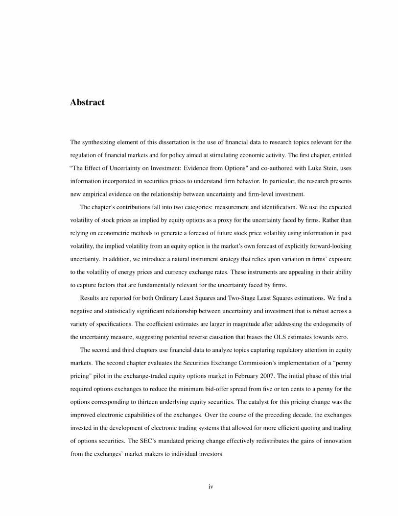
The mean investment-capital ratio in our data sample is 5.2%, with a standard deviation of 6.5%. As

illustrated in Figure 1.1, we observe very little disinvestment and the mass of firms with zero investment in a

given quarter is relatively small. The rarity of zero investment seems to be at odds with a story of irreversible

investment or fixed costs, but aggregation over time and across plants within a firm can help reconcile these

(see Bloom et al., 2007). Another possibility is that the costs incurred to replace depreciated capital may be

less than those incurred for the installation of new capital. As a result, we may observe small amounts of

investment each quarter as firms replace depreciated capital.

As illustrated in Figure 1.1, 91-day implied volatility varies significantly across firms and time, with an

average value of 0.52 and a standard deviation of 0.24.6 Implied volatility is a measure of the annualized

standard deviation of expected returns; the mean observation of 0.52 corresponds to a daily expected standard

deviation of 3.3%. Ideally, we would like to make use of the richness of the options data to evaluate the

importance of different uncertainty durations. For example, is 730-day implied volatility more relevant for

investment decisions than 91-day implied volatility? Unfortunately, the strong correlation between implied

volatilities of different durations makes it difficult to separately identify their roles. Given this high correlation

and the significant amount of new information relevant for investment decisions that is likely to be revealed

within a window of three months, we believe it is reasonable to rely upon 91-day implied volatility for the

majority of our analysis. An added benefit is the fact that implied volatilities of shorter duration options are

more consistently populated in the Option Metrics data. Additional information regarding our data sources is

provided in Appendix 1.8.1.

One potential concern is that firms with equity options may be unrepresentative of the average publicly-

traded firm in the United States. Table 1.1 reports summary statistics comparing firm characteristics for the full

universe of Compustat firms to those of the firms in the merged Compustat-Option Metrics data set. The firms

in the merged data set are approximately three times larger in terms of average sales, market capitalization,

and capital stock. This is consistent with the fact that larger, more established firms are more likely to have

6As illustrated in Appendix 1.8.1, there is substantial cross-sectional variation in implied volatility within each quarter.

6

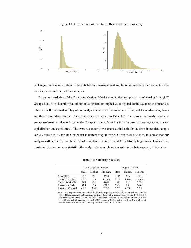
Figure 1.1: Distributions of Investment Rate and Implied Volatility

exchange-traded equity options. The statistics for the investment-capital ratio are similar across the firms in

the Compustat and merged data samples.

Given our restriction of the Compustat-Options Metrics merged data sample to manufacturing firms (SIC

Groups 2 and 3) with a prior year of non-missing data for implied volatility and Tobin’s q, another comparison

relevant for the external validity of our analysis is between the universe of Compustat manufacturing firms

and those in our data sample. These statistics are reported in Table 1.2. The firms in our analysis sample

are approximately twice as large as the Compustat manufacturing firms in terms of average sales, market

capitalization and capital stock. The average quarterly investment-capital ratio for the firms in our data sample

is 5.2% versus 6.0% for the Compustat manufacturing universe. Given these statistics, it is clear that our

analysis will be focused on the effect of uncertainty on investment for relatively large firms. However, as

illustrated by the summary statistics, the analysis data sample retains substantial heterogeneity in firm size.

Table 1.1: Summary Statistics

Full Compustat Universe Merged Data Set

Mean Median Std. Dev. Mean Median Std. Dev.

Sales ($M) 422 24 2334 1,172 210 4,111Market Cap. ($M) 2,029 111 11,886 6,107 1,144 21,054Capital Stock ($M) 795 24 5,069 1,926 215 7,504Investment ($M) 32.1 0.9 221.0 79.2 9.0 340.2Investment/Capital 6.8% 3.3% 12.9% 6.7% 4.3% 9.2%

Note: The Compustat data sample includes 17,322 companies and 454,209 quarterly observations for1996–2009, averaging 26 observations per firm. Out of all investment observations, 2.5% (11,213)are negative and 10.0% (45,360) are zero. The merged data sample includes 5,470 companies and111,808 quarterly observations for 1996–2009, averaging 20 observations per firm. Out of all invest-ment observations, 0.9% (1056) are negative and 2.5% (2,807) are zero.

7

Table 1.2: Summary Statistics – Manufacturing

Compustat Manufacturing Analysis Data Sample

Mean Median Std. Dev. Mean Median Std. Dev.

Sales ($M) 479 23 2,881 1,155 226 3,855Market Cap. ($M) 2,304 111 13,000 7,240 1,237 23,392Capital Stock ($M) 778 23 5,837 1,648 249 5,941Investment ($M) 30.2 0.8 258.5 62.0 9.0 280.2Investment/Capital 6.0% 3.0% 11.6% 5.2% 3.6% 6.5%

Note: The Compustat manufacturing data sample (SIC Groups 2 and 3) includes 6,045 companies and175,704 quarterly observations for 1996–2009, averaging 29 observations per firm. Out of all invest-ment observations, 2.3% (4,115) are negative and 6.4% (11,181) are zero. The analysis data sampleincludes 1,807 manufacturing companies with a prior year of non-missing data for implied volatilityand Tobin’s q. There are 35,835 quarterly observations for 1996–2009, averaging 20 observationsper firm. Out of all investment observations, 0.6% (227) are negative and 0.4% (131) are zero.

1.5 “Naïve” Estimation

For the purpose of exposition, we begin by describing our analysis process and reporting results for a reduced-

form regression of investment on uncertainty that captures covariances but does not allow causal interpretation,

since it fails to account for the likely endogeneity of our uncertainty measure. The dependent variable is the

ratio of a firm’s quarterly investment to its capital stock (Ii,t/Ki,t ). Financial statements report capital at book

value rather than replacement value. Therefore we derive Ki,t recursively using the perpetual inventory method

described in Salinger and Summers (1993), starting from the earliest observation available in Compustat for

each company:

Ki,0 = PPEi,0

Ki,t =πt

πt−1(1−δt)Ki,t−1 + Ii,t

where PPE is Property, Plant and Equipment, and π and δ are the price level and depreciation rate, respectively.7

The regression specification is as follows:

Ii,t

Ki,t= βσ ·σd

i,t−1 +βq ·qi,t−1 + ct + fi + εi,t (1.1)

where σdi,t−1 is the average implied volatility from options with a time horizon of d across all trading days in

the previous quarter (i.e., t−1). This is derived as described in Appendix 1.8.1 from listed equity options on

firm i’s stock that expire in d days. In using the lagged value of implied volatility, we are assuming that the

cash flow associated with a firm’s investment decision does not appear on the company’s financial statements

until the following quarter. This timing assumption allows for a variety of plausible factors including (1) a

7We use the Producer Price Index for Finished Capital Equipment Goods as a measure of the relevant price level and assume a quarterlydepreciation rate of 2.5 percent.

8

delay between a manager’s observation of uncertainty over expected profitability and her resulting investment

decision, (2) time to build, and (3) time to pay given typical invoice deadlines of 60–90 days. We perform a

variety of robustness checks that allow for adjustments to this timing assumption; the results are reported in

Appendix 1.8.2.

Much of the existing literature posits that uncertainty affects investment though marginal Tobin’s q, that

is, the ratio between the value and cost of an additional unit of capital.8 This relationship is highlighted by

Dixit and Pindyck (1994), who show that in the presence of investment irreversibility, uncertainty affects the

threshold value of q at which firms choose to invest. In particular, a higher degree of uncertainty increases the

threshold value of q above which investment occurs.9 A persistent challenge throughout the literature is the

lack of a suitable empirical measure of marginal q. We face the same problem and adopt the common measure

of average Tobin’s q, calculated as the ratio of the market value of the firm’s capital stock to the replacement

cost of the capital:10

q =Debt+Market Capitalization−Current Assets

K + Inventory+ Intangibles+ Investment & Advances

Including q as an explanatory variable serves two purposes. First, q is a natural control for the first moment

effect of the expected return on capital on firms’ investment decisions. Without such a control, our estimates

would suffer from omitted variable bias. Second, the inclusion of q allows us to compare our results with

those found by other researchers. For example, Leahy and Whited (1996) find a positive relationship between

Tobin’s q and investment and a negative relationship between uncertainty (proxied by stock price volatility

forecasts based on realized returns) and investment when each explanatory variable is considered separately;

however, when both q and uncertainty are included in the regression specification, they find that neither

coefficient estimate is statistically significant.11 With these prior findings in mind, we test whether uncertainty

and Tobin’s q have a role in driving investment patterns when we improve upon both the measurement of

uncertainty and the identification strategy.12

8Abel and Eberly (1994) note that marginal q is equivalent to the expected present value of the stream of marginal products of capital in amultiperiod model.

9In addition, Abel and Eberly (1994) develop a model that nests the model of Abel (1983) and an irreversible investment model. Theyshow that under general assumptions investment depends only on marginal q and the capital stock; that is, uncertainty affects investmentonly through marginal q.

10Perfect competition and constant returns to scale are necessary—though not sufficient—for average q and marginal q to be equal (seeHayashi, 1982).

11Leahy and Whited (1996) interpret this finding as evidence that uncertainty operates through the first moment of returns. However,it is important to emphasize that such a conclusion is not technically possible using this empirical test. Recall that in a world withconstant returns to scale and perfect competition, uncertainty has no effect on investment. As illustrated in Dixit and Pindyck (1994),without these conditions, uncertainty only affects investment through marginal q. In the absence of constant returns to scale or perfectcompetition, marginal q is not equal to average q. Therefore, an empirical specification using average q cannot conclusively test thetheory’s prediction that the effect of uncertainty on investment operates exclusively through marginal q.

12Kogan (2004) examines the direct relationship between Tobin’s q and stock price volatility. His general equilibrium model predicts anon-linear relationship between q and asset price volatility as prices absorb demand shocks in some states of the world. As suggestedby these predictions, we estimate the relationship between our implied volatility and Tobin’s q data series and find evidence of such

9

We estimate Equation 1.1 in first differences to eliminate the firm fixed effects ( fi) and to address the serial

correlation between consecutive error terms in the levels equation. All specifications include time controls to

capture the effect of the macroeconomic environment on firm investment. In some specifications, we include

the level of the S&P 500 Index, while in others we take a non-parametric approach and include quarterly time

fixed effects (ct ). As mentioned earlier, the instrumental variable estimates we present in the next section rely

on data that is only available for manufacturing firms (SIC Groups 2 and 3). As a result, we restrict our sample

to these 2,230 firms to ensure the Ordinary and Two-Stage Least Squares results are comparable. In addition,

we require the firms in our sample to have a prior year of non-missing data for both Tobin’s q and implied

volatility. This further reduces the sample to 1,807 firms and 35,835 observations. We report Ordinary Least

Squares results for the full Compustat-Option Metrics merged data set in Appendix 1.8.5.

As reported in Table 1.3, we find a negative and strongly statistically significant coefficient estimate of

−0.0282 for uncertainty as measured by the change in the one-quarter lag of 91-day implied volatility. Given

a standard deviation of implied volatility of 0.24 in our data sample, a one standard deviation increase in

uncertainty is associated with a 0.7% decline in the quarterly investment rate. The average firm in our sample

has an investment rate of 5.2%. Thus, this decrease is equivalent to an economically significant decrease in

investment of 13.0% for the average firm.

Table 1.3: OLS Regressions

(1) (2) (3) (4) (5) (6)D.I/K D.I/K D.I/K D.I/K D.I/K D.I/K

LD.91d vol -0.0282∗∗∗ -0.0242∗∗∗ -0.0235∗∗∗ -0.0176∗∗∗ -0.0189∗∗∗ -0.0120∗

(0.00496) (0.00500) (0.00607) (0.00621) (0.00640) (0.00658)

LD.Tobin’s q 0.00233∗∗∗ 0.00237∗∗∗ 0.00237∗∗∗

(0.000362) (0.000364) (0.000365)

LD.SPX level -0.0000117∗∗∗ -0.0000212∗∗∗ -0.0000157∗∗∗ -0.0000268∗∗∗

(0.00000369) (0.00000369) (0.00000402) (0.00000411)

LD.SPX 91d vol -0.0211∗∗ -0.0292∗∗∗

(0.0104) (0.0106)

Quarterly fixed effects X X

N 35835 35835 35835 35835 35835 35835∗ p < 0.10, ∗∗ p < 0.05, ∗∗∗ p < 0.01. Standard errors clustered by firm are reported in parentheses.

Note: Sample includes quarterly observations 1/1996–10/2009 for manufacturing (SIC Groups 2 and 3) firms with a prior year of data for impliedvolatility and Tobin’s q. The dependent variable is the quarterly change (“D”) in a firm’s investment rate (I/K). Explanatory variables includethe lagged differences (“LD”) of 91-day implied volatility from the firm’s equity options (“91d vol”), Tobin’s q, and the level and options-implied volatility of the S&P 500 Index (“SPX level” and “SPX 91d vol”). Quarterly time fixed effects are included in some specifications(denoted by a checkmark).

non-linearities. The results of this exercise are presented in Appendix 1.8.7.

10

When included as an additional explanatory variable, the coefficient estimate for Tobin’s q is positive and

statistically significant. Consistent with findings elsewhere in the literature, the coefficient estimate of 0.00233

implies an unreasonably large adjustment cost (equal to the reciprocal of the coefficient on q). This is likely

due to the susceptibility of the numerator in the calculation of Tobin’s q to market bubbles and noise. In strong

contrast to the findings of Leahy and Whited (1996), when both Tobin’s q and the uncertainty measure are

included in the specification, the negative coefficient estimate for uncertainty and positive coefficient estimate

for Tobin’s q remain statistically significant (with p-values of less than one percent). As we would expect

if a portion of the effect of uncertainty on investment operates through the first-moment effect of expected

returns, the coefficient estimate for implied volatility is smaller in magnitude when Tobin’s q is included in the

regression specification.

Specifications (3) and (4) include the implied volatility from S&P 500 Index options as a control for

market-wide, systematic uncertainty, allowing us to isolate the relationship between changes in firm-specific

idiosyncratic uncertainty and changes in investment. The coefficient estimate for S&P 500 implied volatility

indicates a negative relationship between market-wide uncertainty and firm-level investment. This is consistent

with the observation that market implied volatility tends to increase in periods of recession; periods when firm

investment typically declines.13

Controlling for systematic uncertainty, we find a negative and statistically significant coefficient estimate for

idiosyncratic uncertainty regardless of whether Tobin’s q is included. Given a standard deviation of 0.07 for the

91-day implied volatility of the S&P 500 Index, a one standard deviation increase in market-wide uncertainty

is associated with a 0.1% decline in a firm’s investment rate. The estimated relationship between systematic

uncertainty and investment is therefore smaller than the relationship between idiosyncratic uncertainty and

investment, according to which a one standard deviation increase in uncertainty is associated with a 0.6%

decrease in the investment rate.

To emphasize the pivotal role played by our use of implied volatility as a proxy measure of uncertainty,

we perform the same analysis using the realized volatility of stock returns. We calculate quarterly realized

volatility for each firm as the average of the rolling 90-day standard deviation of daily returns across all of the

trading days in each quarter. (The timing is thus consistent with our quarterly measure of implied volatility.)

Figure 1.2 presents the distributions of 91-day implied volatility and realized volatility in our data sample. The

implied and realized volatility measures have the same mean (0.52), but realized volatility has a slightly higher

standard deviation (0.28 versus 0.24 for implied volatility) and a higher kurtosis (10.4 versus 5.0 for implied

13Note that with time-varying volatility and risk-averse investors, option-implied volatility is the sum of expected volatility and a riskpremium. Risk premia vary over time and tend to be countercyclical. In a regression of investment on option-implied volatility, anegative coefficient may therefore reflect firms’ responses to high risk premia rather than to increases in uncertainty. Assuming the riskpremium is a primarily macroeconomic variable, the inclusion of time fixed effects or S&P 500 implied volatility controls for the effectof changing risk premia on firm investment patterns.

11

Figure 1.2: Distributions of Implied and Realized Volatility

volatility). As kurtosis is a measure of the peakedness of the distribution, the higher kurtosis for realized

volatility means that more of its variance is the result of infrequent extreme deviations, as opposed to frequent

modestly sized deviations. This is consistent with the observation that implied volatility is often a smoother

(and less noisy) series than realized volatility (Schwert, 2002).

Table 1.4 reports results for Ordinary Least Squares estimation of the first-differences of Equation 1.1,

where σdi,t−1 is now realized rather than implied volatility. In the regression specifications that include the

level of the S&P 500 Index as a time control, the coefficient estimates for realized volatility are negative and

statistically significant, although less than one-third the size of the estimated coefficients for implied volatility.

In the specifications including the volatility of the S&P 500 Index or quarterly time fixed effects, the coefficient

estimates on firm-specific realized volatility are neither economically nor statistically significant. Furthermore,

when both implied volatility and realized volatility are included in the regression specification, the coefficient

on implied volatility is negative and statistically significant while the coefficient on realized volatility is neither

economically nor statistically significant. These estimation results are reported in Appendix 1.8.6. Based on

these findings, realized volatility is not nearly as strong a predictor of investment as implied volatility.

12

Table 1.4: OLS Regressions – Realized Volatility

(1) (2) (3) (4) (5) (6)D.I/K D.I/K D.I/K D.I/K D.I/K D.I/K

LD.Realized vol -0.00823∗∗∗ -0.00815∗∗∗ 0.000737 0.00123 0.000699 0.00146(0.00296) (0.00292) (0.00335) (0.00332) (0.00338) (0.00336)

LD.Tobin’s q 0.00245∗∗∗ 0.00249∗∗∗ 0.00244∗∗∗

(0.000362) (0.000363) (0.000363)

LD.SPX level -0.00000661∗ -0.0000176∗∗∗ -0.0000167∗∗∗ -0.0000284∗∗∗

(0.00000359) (0.00000353) (0.00000394) (0.00000400)

LD.SPX realized vol -0.0448∗∗∗ -0.0468∗∗∗

(0.00620) (0.00623)

Quarterly fixed effects X X

N 35835 35835 35835 35835 35835 35835∗ p < 0.10, ∗∗ p < 0.05, ∗∗∗ p < 0.01. Standard errors clustered by firm are reported in parentheses.

Note: Sample includes quarterly observations 1/1996–10/2009 for manufacturing (SIC Groups 2 and 3) firms with a prior year of data forimplied volatility, realized volatility, and Tobin’s q. The dependent variable is the quarterly change (“D”) in a firm’s investment rate (I/K).Explanatory variables include the lagged differences (“LD”) of average realized volatility of the firm’s stock price (“Realized vol”), Tobin’sq, and the level and average realized volatility of the S&P 500 Index (“SPX level” and “SPX realized vol”). Quarterly time fixed effects areincluded in some specifications (denoted by a checkmark).

1.6 Instrumental Variables Estimation

1.6.1 Endogeneity of Uncertainty

While we are interested in the effect of uncertainty on investment, the reverse relationship is likely also

relevant, with investment decisions driving the degree of uncertainty. For example, if a firm undertakes a risky

investment project, the observed implied volatility may increase to reflect the subsequently greater uncertainty

regarding future returns.14 Given the endogeneity of both investment and uncertainty, an instrumental variables

strategy is necessary. Much of the existing literature addresses this issue by using lagged values of the

dependent and explanatory variables as instruments (following the methodology of Arellano and Bond, 1991).

Instead, we suggest a natural instrument strategy and construct industry-specific exposures to energy and

currency volatility as proxies for exogenous uncertainty shocks.

In particular, following Rajan and Zingales (1998), the instruments are structured as the product of

predetermined cross-sectional intensity and time-varying volatility:

Exposurei,t ≡ Intensityi ·Volatilityt (1.2)

The instruments rely upon cross-sectional variation in predetermined measures of energy intensity-of-use and

country-specific trade volume. The role of trade volume can be thought of as follows: import trade volume in

a given industry captures foreign competition with the industry’s goods, and export trade volume captures

14Another potential source of endogeneity is the presence of a latent third factor that affects both investment and uncertainty.

13

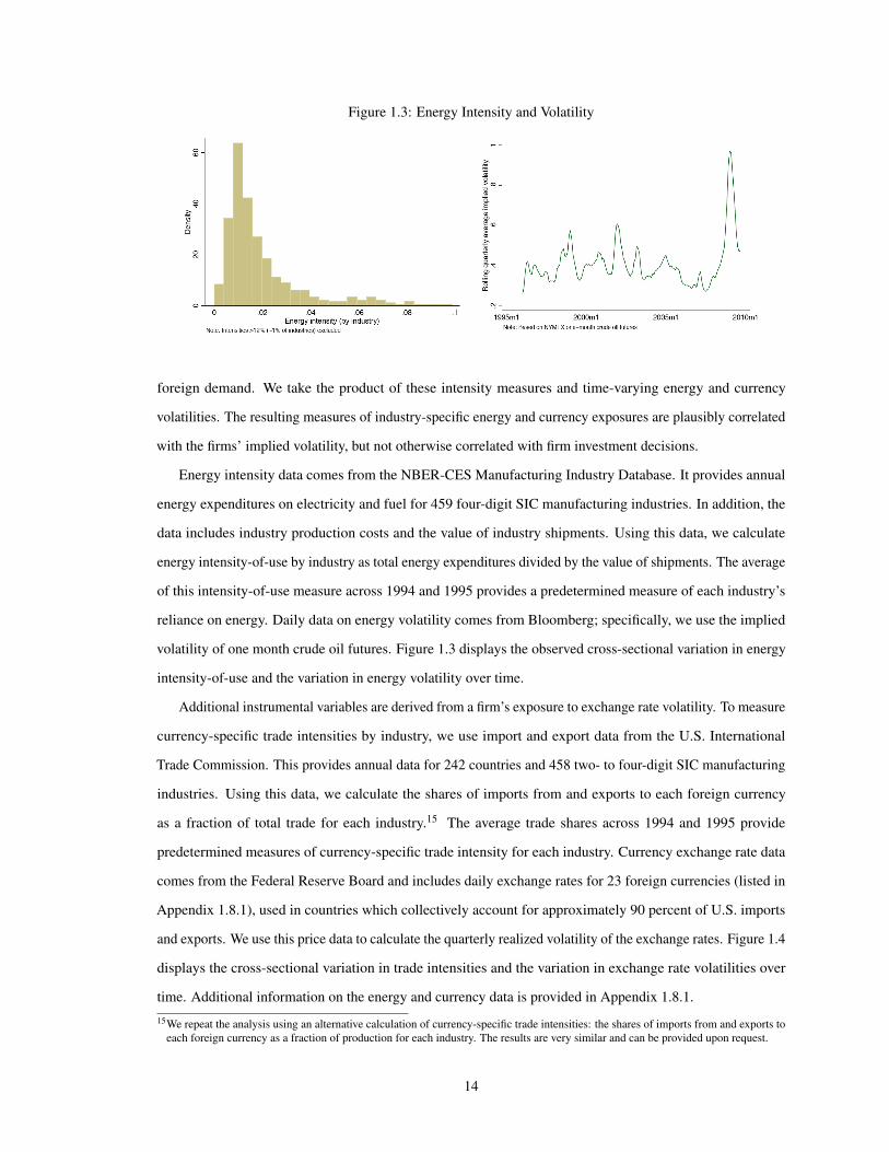
Figure 1.3: Energy Intensity and Volatility

foreign demand. We take the product of these intensity measures and time-varying energy and currency

volatilities. The resulting measures of industry-specific energy and currency exposures are plausibly correlated

with the firms’ implied volatility, but not otherwise correlated with firm investment decisions.

Energy intensity data comes from the NBER-CES Manufacturing Industry Database. It provides annual

energy expenditures on electricity and fuel for 459 four-digit SIC manufacturing industries. In addition, the

data includes industry production costs and the value of industry shipments. Using this data, we calculate

energy intensity-of-use by industry as total energy expenditures divided by the value of shipments. The average

of this intensity-of-use measure across 1994 and 1995 provides a predetermined measure of each industry’s

reliance on energy. Daily data on energy volatility comes from Bloomberg; specifically, we use the implied

volatility of one month crude oil futures. Figure 1.3 displays the observed cross-sectional variation in energy

intensity-of-use and the variation in energy volatility over time.

Additional instrumental variables are derived from a firm’s exposure to exchange rate volatility. To measure

currency-specific trade intensities by industry, we use import and export data from the U.S. International

Trade Commission. This provides annual data for 242 countries and 458 two- to four-digit SIC manufacturing

industries. Using this data, we calculate the shares of imports from and exports to each foreign currency

as a fraction of total trade for each industry.15 The average trade shares across 1994 and 1995 provide

predetermined measures of currency-specific trade intensity for each industry. Currency exchange rate data

comes from the Federal Reserve Board and includes daily exchange rates for 23 foreign currencies (listed in

Appendix 1.8.1), used in countries which collectively account for approximately 90 percent of U.S. imports

and exports. We use this price data to calculate the quarterly realized volatility of the exchange rates. Figure 1.4

displays the cross-sectional variation in trade intensities and the variation in exchange rate volatilities over

time. Additional information on the energy and currency data is provided in Appendix 1.8.1.

15We repeat the analysis using an alternative calculation of currency-specific trade intensities: the shares of imports from and exports toeach foreign currency as a fraction of production for each industry. The results are very similar and can be provided upon request.

14

Figure 1.4: Currency Intensity and Volatility

05

100

510

05

100

510

0 .2 .4 .6 .8

Canadian Dollar

Euro

Japanese Yen

Mexican Peso

Den

sity

Export share (by industry)

These measures of exposure to energy and currency volatility are used as explanatory variables in the

following first-stage regression:

σi,t = αoil ·(

Eiσoilt

)+αimp ·

(∑

jw j,imp

i σj/USD

t

)+αexp ·

(∑

jw j,exp

i σj/USD

t

)+ ct + fi +ηi,t (1.3)

where Ei is the intensity of energy use for firm i’s industry and σoilt is the implied volatility of one-month

crude oil futures in quarter t. For the currency instruments, w ji σ

j/USDt is the trade-weighted realized volatility

of the exchange rate between the U.S. dollar and j’s currency in quarter t. For example, w j,impi is the fraction

of all imports in firm i’s industry that come from countries using currency j, and w j,expi is the fraction of all

exports from firm i’s industry that go to countries using currency j. The estimation includes time controls

(either the level of the S&P 500 Index or quarterly time fixed effects, ct ) and firm fixed effects ( fi), which are

especially important to capture heterogeneity in the relationship between implied volatility and exposure to

energy volatility.16

The results of the estimation of Equation 1.3 in first-differences are reported in Table 1.5 for an implied

volatility duration of 91 days. Each of the instruments is positively correlated with changes in implied volatility,

as expected, and the relationships are strongly statistically significant. For example, in specification (2), a

one percent increase in the oil exposure variable (intensity of energy use multiplied by oil price volatility)

is associated with a 6.1 percent increase in a firm’s implied volatility, holding all else constant. Further

confirming the strength of the instruments, the F-statistic for the joint test that the instruments’ coefficients are

equal to zero is well above the commonly referenced hurdle value of ten.17 In addition, as evidenced by the

16Without firm fixed effects, the overall relationship between implied volatility and the energy exposure instrument is negative. However,this is driven by extreme differences in implied volatilities and energy exposures across industries. For example, the computer gamingindustry has high implied volatility from equity options but very low exposure to energy volatility, while the concrete industry has lowimplied volatility from equity options but high exposure to energy volatility. While the relationship between implied volatility andenergy exposure may be positive within each industry, the relationship across industries is negative.

17Stock and Yogo (2005) provide critical values for a test of weak instruments in linear instrumental variables estimation. Given a single

15

reported R-squared values, the uncertainty instruments explain between 20 and 36 percent of the variation in

firm-specific implied volatility.

Table 1.5 also reports results for a specification that includes the implied volatility from S&P 500 Index

options as an additional control. Controlling for market-wide uncertainty drastically changes the estimated

coefficients on the currency instruments. The coefficient for import uncertainty shocks is economically and

statistically indistinguishable from zero and the coefficient for export uncertainty shocks is negative. These

changes are likely driven by the high correlation between market-wide uncertainty and the volatility of currency

prices.

Table 1.5: Volatility Partial First Stage

Hypothesis (1) (2) (3) (4)D.91d vol D.91d vol D.91d vol D.91d vol

D.Import curr vol shock + 0.416∗∗∗ 0.350∗∗∗ -0.0289 0.140∗∗∗

(0.0591) (0.0562) (0.0381) (0.0424)

D.Export curr vol shock + 1.008∗∗∗ 0.916∗∗∗ -0.208∗∗∗ 0.509∗∗∗

(0.0586) (0.0567) (0.0435) (0.0698)

D.Oil vol shock + 6.390∗∗∗ 6.124∗∗∗ 2.191∗∗∗ 2.516∗∗∗

(0.635) (0.619) (0.352) (0.449)

D.SPX level -0.000101∗∗∗ 0.0000456∗∗∗

(0.00000612) (0.00000593)

D.SPX 91d vol 1.321∗∗∗

(0.0223)

Quarterly fixed effects X

N 35835 35835 35835 35835F: All instruments = 0 1087.7 808.3 36.96 41.21R-squared 0.197 0.205 0.327 0.364∗ p < 0.10, ∗∗ p < 0.05, ∗∗∗ p < 0.01. Standard errors clustered by firm are reported in parentheses.

Note: Sample includes quarterly observations 1/1996–10/2009 for manufacturing (SIC Groups 2 and 3) firms with aprior year of data for implied volatility and Tobin’s q. The dependent variable is the quarterly change (“D”) in the91-day implied volatility from a firm’s equity options (“91d vol”). Explanatory variables include the changes inthe currency and energy volatility exposure instruments as well as in the level and options-implied volatility of theS&P 500 Index (“SPX level” and “SPX 91d vol”). Quarterly time fixed effects are included in some specifications(denoted by a checkmark).

1.6.2 Endogeneity of Tobin’s q

As with uncertainty, the exogeneity of Tobin’s q is unlikely. Again, much of the existing literature addresses

this issue by using lagged values of the dependent and explanatory variables as instruments. Instead, we pursue

a natural instrument strategy similar to what we use for uncertainty, but use industry-specific exposures to

energy and currency prices—rather than volatilities—as proxies for exogenous profitability shocks.

endogenous variable and three excluded instruments, a critical value of ten corresponds to a five to ten percent bias of the IV estimatorrelative to the OLS estimator and a Wald test size of fifteen to twenty percent.

16

The instruments for Tobin’s q are structured as:

Exposurei,t ≡ Intensityi ·Pricet (1.4)

The predetermined measures of cross-sectional energy intensity-of-use and currency-specific trade shares

are the same as those used for the volatility instruments. We take the product of the intensity measures and

time-varying energy and currency prices.18 The resulting measures of industry-specific energy and currency

exposures are plausibly correlated with the expected return on capital captured by a firm’s value of Tobin’s q,

but not otherwise correlated with the firm’s investment decisions.

Partial first stage results are reported in Table 1.6 (partial in the sense that the formal first-stage regression

will include the full set of both volatility and Tobin’s q instruments). We expect the coefficients for the import

and export instruments to be negative. An increase in the exchange rate is a depreciation of the foreign currency

relative to the U.S. dollar. This makes imports into the U.S. relatively cheap, hurting firms’ competitive position

relative to foreign firms. It also hurts the ability of domestic firms to sell their products abroad. Consistent

with these stories, we find negative and statistically significant coefficient estimates for the import and export

instrumental variables.

We also expect the coefficient on the energy instrument to be negative: a firm in an industry that uses

energy more intensively is expected to be less profitable when oil prices rise. Again, the results are consistent

with this prediction. The coefficient estimate on the energy instrument is negative and strongly statistically

significant after controlling for quarterly time effects. In all four first-stage specifications (with and without

quarterly time fixed effects, as well as with controls for the level and implied volatility of the S&P 500 Index),

the instrument variables for Tobin’s q are jointly significant with F-statistics well above ten. The reported

R-squared values range from 0.2 to 9 percent. The fact that we explain only a small fraction of the variation in

Tobin’s q is not surprising given the multitude of factors relevant for expected stock price returns. Exposures

to energy and currency prices are likely only a small subset of these potential factors.

The complete first-stage regression results are reported in Table 1.7. The full instrument set includes the

instruments for both implied volatility and Tobin’s q. Given the exogeneity of each group of instruments,

the combined set is jointly exogenous. All of the findings highlighted in the tables looking separately at the

validity of the instruments for implied volatility and Tobin’s q carry over to the full first-stage regression.19

18The crude oil price series used for the energy instrument is the deseasoned natural logarithm of the deflated price series provided byBloomberg.

19Stock and Yogo (2005) provide critical values for a test of weak instruments in linear instrumental variables estimation. Given twoendogenous variables and six excluded instruments, a critical value of ten corresponds to a five to ten percent bias of the IV estimatorrelative to the OLS estimator and a Wald test size of fifteen to twenty percent.

17

Table 1.6: Tobin’s q Partial First Stage

Hypothesis (1) (2) (3) (4)D.Tobin’s q D.Tobin’s q D.Tobin’s q D.Tobin’s q

D.Import curr price shock - -0.00971∗∗∗ -0.00592∗∗∗ -0.00596∗∗∗ -0.00833∗∗∗

(0.00174) (0.00168) (0.00168) (0.00180)

D.Export curr price shock - -0.00810∗∗∗ 0.000260 0.0000529 -0.00787∗∗∗

(0.00158) (0.00164) (0.00165) (0.00181)

D.Oil price shock - 6.592∗∗∗ -8.667∗∗∗ -7.999∗∗∗ -6.421∗∗∗

(1.292) (1.539) (1.483) (1.652)

D.SPX level 0.00443∗∗∗ 0.00449∗∗∗

(0.000152) (0.000173)

D.SPX 91d vol 0.259(0.241)

Quarterly fixed effects X

N 35835 35835 35835 35835F: All instruments = 0 49.74 14.62 14.30 20.07R-squared 0.00248 0.0590 0.0591 0.0868∗ p < 0.10, ∗∗ p < 0.05, ∗∗∗ p < 0.01. Standard errors clustered by firm are reported in parentheses.

Note: Sample includes quarterly observations 1/1996–10/2009 for manufacturing (SIC Groups 2 and 3) firms with a prioryear of data for implied volatility and Tobin’s q. The dependent variable is the quarterly change (“D”) in a firm’s Tobin’sq. Explanatory variables include the changes in the currency and energy price exposure instruments as well as in thelevel and options-implied volatility of the S&P 500 Index (“SPX level” and “SPX 91d vol”). Quarterly time fixed effectsare included in some specifications (denoted by a checkmark).

1.6.3 Two-Stage Least Squares Results

Using the fitted values from the first-stage regressions for volatility and Tobin’s q, we estimate the following

second-stage regression:Ii,t

Ki,t= βσ · σ̂d

i,t−1 +βq · q̂i,t−1 + ct + fi + εi,t

The results are reported in Table 1.8. In specifications (1) and (2), we control for time effects using the

level of the S&P 500 Index. Here, we find a negative and strongly statistically significant coefficient on

firm-specific implied volatility. Importantly, the coefficient estimates are larger in magnitude than the OLS

estimates presented in Section 1.5. This is evidence of potential reverse causation. Suppose a firm undertakes

an investment project and the market does not know whether this is a high or low quality investment. This

uncertainty regarding future returns will be reflected in a higher expected volatility of the firm’s stock price. In

this scenario, the OLS estimates will be biased towards zero since they fail to account for the endogeneity of

the uncertainty measure.

Specifications (3) and (4) include the implied volatility of the S&P 500 Index as a measure of market-

wide uncertainty. Recall that the inclusion of S&P 500 implied volatility generates surprising coefficient

estimates for the currency instruments in the first-stage regressions. As a result, we are hesitant to draw

strong conclusions from the results for these specifications. However, with this qualification in mind, it is

valuable to highlight the dramatically different effects of idiosyncratic versus systematic uncertainty. The

18

Table 1.7: Full First Stage Regression

(1) (2) (3) (4) (5) (6)D.Tobin’s q D.Tobin’s q D.Tobin’s q D.91d vol D.91d vol D.91d vol

D.Import curr vol shock 1.856∗∗∗ 2.004∗∗∗ -1.232∗ 0.350∗∗∗ -0.0408 0.126∗∗∗

(0.678) (0.698) (0.678) (0.0565) (0.0387) (0.0434)

D.Export curr vol shock -0.781 -0.346 -2.667∗∗∗ 0.915∗∗∗ -0.231∗∗∗ 0.486∗∗∗

(0.624) (0.669) (0.836) (0.0573) (0.0449) (0.0720)

D.Oil vol shock 8.268∗∗∗ 9.428∗∗∗ 10.20∗∗∗ 5.495∗∗∗ 2.442∗∗∗ 2.387∗∗∗

(2.443) (2.415) (2.823) (0.555) (0.341) (0.416)

D.Import curr price shock -0.00668∗∗∗ -0.00676∗∗∗ -0.00740∗∗∗ -0.0000128 0.000175∗ 0.000286∗∗

(0.00164) (0.00164) (0.00179) (0.000118) (0.0000990) (0.000112)

D.Export curr price shock -0.000319 -0.000469 -0.00658∗∗∗ 0.00000751 0.000404∗∗∗ 0.000343∗∗

(0.00159) (0.00159) (0.00181) (0.000140) (0.000127) (0.000161)

D.Oil price shock -4.655∗∗∗ -5.027∗∗∗ -3.121∗ -0.627∗∗∗ 0.352∗∗∗ -0.174(1.438) (1.472) (1.713) (0.149) (0.127) (0.145)

D.SPX level 0.00456∗∗∗ 0.00450∗∗∗ -0.000100∗∗∗ 0.0000469∗∗∗

(0.000163) (0.000173) (0.00000609) (0.00000590)

D.SPX 91d vol -0.505 1.330∗∗∗

(0.361) (0.0225)

Quarterly fixed effects X X

N 35835 35835 35835 35835 35835 35835F: All instruments = 0 10.79 11.36 12.86 406.5 25.52 23.35R-squared 0.0594 0.0595 0.0873 0.206 0.328 0.364∗ p < 0.10, ∗∗ p < 0.05, ∗∗∗ p < 0.01. Standard errors clustered by firm are reported in parentheses.

Note: Sample includes quarterly observations 1/1996–10/2009 for manufacturing (SIC Groups 2 and 3) firms with a prior year of data forimplied volatility and Tobin’s q. The dependent variable is the quarterly change (“D”) in a firm’s Tobin’s q in columns (1)–(3), and in the91-day implied volatility from its equity options (“91d vol”) in columns (4)–(6). Explanatory variables include the changes in the currencyand energy volatility and price exposure instruments as well as in the level and options-implied volatility of the S&P 500 Index (“SPX level”and “SPX 91d vol”). Quarterly time fixed effects are included in some specifications (denoted by a checkmark).

implied volatility of S&P 500 Index options has a positive and statistically significant coefficient, suggesting a

positive relationship between market-wide uncertainty and firm investment after controlling for idiosyncratic

uncertainty.

In specifications (5) and (6), we include quarterly time fixed effects rather than controls for the level and

implied volatility of the market. After removing all common time variation in the first-stage regression, the

instrumental variables estimation does not have sufficient power to generate precise estimates for the effect of

firm-specific uncertainty. In other words, there is not enough variation among the first-stage fitted values. This

is evidenced by the large standard errors for the 2SLS estimates. Given the magnitude of the standard errors,

we cannot reject that the coefficient estimate of 0.0223 in specification (5) is statistically different from the

estimate of −0.0483 in specification (1).

19

Table 1.8: Two-Stage Least Squares Estimation

(1) (2) (3) (4) (5) (6)D.I/K D.I/K D.I/K D.I/K D.I/K D.I/K

LD.91d vol -0.0483∗∗∗ -0.0608∗∗∗ -0.128∗∗∗ -0.158∗∗∗ 0.0223 0.0251(0.00751) (0.00890) (0.0421) (0.0452) (0.0352) (0.0302)

LD.Tobin’s q 0.0147∗∗∗ 0.00861∗∗ 0.00390(0.00475) (0.00420) (0.00350)

LD.SPX level -0.0000169∗∗∗ -0.0000862∗∗∗ -0.0000106∗∗∗ -0.0000485∗∗∗

(0.00000388) (0.0000226) (0.00000407) (0.0000187)

LD.SPX 91d vol 0.109∗∗ 0.144∗∗

(0.0528) (0.0565)

Quarterly fixed effects X X

N 35835 35835 35835 35835 35835 35835∗ p < 0.10, ∗∗ p < 0.05, ∗∗∗ p < 0.01. Standard errors clustered by firm are reported in parentheses.

Note: Sample includes quarterly observations 1/1996–10/2009 for manufacturing (SIC Groups 2 and 3) firms with a prior year of data forimplied volatility and Tobin’s q. The dependent variable is the quarterly change (“D”) in a firm’s investment rate (I/K). Explanatoryvariables include the lagged differences (“LD”) of 91-day implied volatility from the firm’s equity options (“91d vol”), Tobin’s q, and thelevel and options-implied volatility of the S&P 500 Index (“SPX level” and “SPX 91d vol”) Firm-specific implied volatility and Tobin’s qare instrumented using exposure to energy and currency volatility and prices. Quarterly time fixed effects are included in some specifications(denoted by a checkmark).

1.7 Conclusion

The results reported in the previous sections provide new evidence on the empirical relationship between

uncertainty and investment at the disaggregated firm level. In pursuing this research objective, we make two

central contributions to the existing literature. First, we introduce the expected volatility of stock prices as

implied by equity options as a proxy for firm-specific uncertainty. This measure captures the market’s forecast

of forward-looking uncertainty and is shown to be a stronger predictor of investment than realized volatility.

Second, we develop an instrumental variables strategy that relies upon firms’ exposure to energy and currency

prices and volatility. The first-stage regression results confirm that these instruments have strong explanatory

power for firm-specific implied volatility.

Using these measurement and identification strategies, we find a negative effect of firm-specific uncertainty

on investment that is both economically and statistically significant. The magnitude of the effect estimated by

Two-Stage Least Squares is larger than that estimated by Ordinary Least Squares. This is evidence of potential

reverse causation, whereby the perceived risk of a firm’s investment decision is incorporated in the implied

volatility of its stock price. As discussed in the summary of the existing empirical literature, previous research

has typically found a weak negative relationship between uncertainty and investment that is often not robust to

the inclusion of additional explanatory variables such as Tobin’s q. We attribute the relative strength of our

results to our novel approaches to measurement and identification.

While we find a strong effect of uncertainty using the level of the S&P 500 Index as a control for

macroeconomic time effects, we lack sufficient power to generate precise estimates when we include quarterly

20

time fixed effects. One potential solution is to retain greater variation among the first-stage fitted values by

introducing additional instrument variables. Exposures to energy and currency volatility are certainly important

elements of overall uncertainty, as evidenced by their strength in the first-stage regressions. However, they

likely capture only a limited subset of all the factors contributing to uncertainty. A goal for future work is to

expand our set of instruments in order to include additional drivers of the uncertainty faced by firms. One

possibility is to draw from the research of Julio and Yook (2009) and use political uncertainty as an instrument.

The results reported in this paper measure the average effect of uncertainty on investment for a sample

of relatively large manufacturing firms. Assessing heterogeneous effects among this sample is a valuable

extension. For example, the effect of uncertainty may vary across industries and firm size. In addition,

evaluating how the effect of uncertainty changes with a firms’ cash holdings can potentially address the role of

financial constraints.

The application of the analysis methodology presented in this paper is certainly not limited to specifications

with investment as the dependent variable. Rather, this methodology will be useful for looking at the effect of

uncertainty on other critical firm-level decisions. For example, uncertainty is likely relevant for employment

decisions and the allocation of funding to research and development projects. Evaluating the effect of

uncertainty on these additional variables is a promising avenue for future research.

21

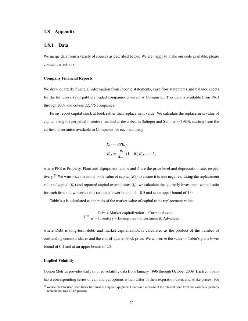
1.8 Appendix

1.8.1 Data

We merge data from a variety of sources as described below. We are happy to make our code available; please

contact the authors.

Company Financial Reports

We draw quarterly financial information from income statements, cash flow statements and balance sheets

for the full universe of publicly traded companies covered by Compustat. This data is available from 1961

through 2009 and covers 22,775 companies.

Firms report capital stock at book rather than replacement value. We calculate the replacement value of

capital using the perpetual inventory method as described in Salinger and Summers (1983), starting from the

earliest observation available in Compustat for each company:

Ki,0 = PPEi,0

Ki,t =πt

πt−1(1−δt)Ki,t−1 + Ii,t

where PPE is Property, Plant and Equipment, and π and δ are the price level and depreciation rate, respec-

tively.20 We winsorize the initial book value of capital (K0) to ensure it is non-negative. Using the replacement

value of capital (Kt ) and reported capital expenditures (It ), we calculate the quarterly investment-capital ratio

for each firm and winsorize this ratio at a lower bound of −0.5 and at an upper bound of 1.0.

Tobin’s q is calculated as the ratio of the market value of capital to its replacement value:

q =Debt+Market capitalization−Current Assets

K + Inventory+ Intangibles+ Investment & Advances

where Debt is long-term debt, and market capitalization is calculated as the product of the number of

outstanding common shares and the end-of-quarter stock price. We winsorize the value of Tobin’s q at a lower

bound of 0.1 and at an upper bound of 20.

Implied Volatility

Option Metrics provides daily implied volatility data from January 1996 through October 2009. Each company

has a corresponding series of call and put options which differ in their expiration dates and strike prices. For

20We use the Producer Price Index for Finished Capital Equipment Goods as a measure of the relevant price level and assume a quarterlydepreciation rate of 2.5 percent.

22

each of these options, Option Metrics imputes an implied volatility for each trading day using the average of

the end-of-day best bid and offer price quotes. Given an option price, duration, and strike price, along with

interest rates, underlying stock price, and dividends, the Black-Scholes formula is used to back out implied

volatility. This is an annualized measure representing the standard deviation of the expected percentage change

in the stock price. Note that this is not a directional measure, but rather an expectation of absolute stock price

movements regardless of their direction.

One of the advantages of using implied volatilities is that they can be measured across a variety of

time horizons using options with different expiration dates. In particular, Option Metrics calculates implied

volatilities for durations ranging from 30 to 730 days.21 We use these implied volatility horizons to measure

uncertainty over different forward-looking periods.

The calculations underlying our data are in fact somewhat more complicated. Option Metrics builds an

“implied volatility surface” for each underlying asset using options across a wide range of both expiration

dates and strike prices. Although only a finite number of options trade for each asset, implied volatilities

for arbitrary durations and strike prices can be calculated by interpolating the implied volatilities of “nearby”

options. For instance, suppose we want the implied volatility for a Microsoft at-the-money call option expiring

in 60 days when the current stock price is $51.50. Unfortunately, 60 days falls in between the expiration of

listed March and June options. In addition, the March and June-expiry options are only listed for strikes of

$50 and $52.50. In order to compute the 60-day at-the-money implied volatility, Option Metrics interpolates

using the available prices for March and June-expiry $50 and $52.50 strike options.

While implied volatility data is available for a variety of strike prices, we restrict our analysis to at-the-

money-forward options; i.e., options for which the strike price is equal to the forward price of the underlying

stock at the given expiration date. The forward (or expected future) price is calculated from the current stock

price, the stock’s dividend payout rate, and the interest rate yield curve. One possible extension of our analysis

would consider implied volatility across a variety of strike prices, allowing richer measurement of asymmetric

volatility expectations.

We further restrict our analysis to call options. Note that a call option and a put option on a given underlying

asset with the same strike price and expiration date have the same implied volatilities; the difference in their

prices comes from the fact that interest rates and dividends affect the value of call and put options in opposite

directions. An analysis that attempted to separately measure upside and downside risk would benefit from

including both puts and calls, since extreme strike prices are likely only to be available as one or the other.

Here we consider only at-the-money-forward options, for which both puts and calls are available. To make

21Specifically, the implied volatility horizons are 30, 60, 91, 122, 152, 182, 273, 365, 573 and 730 days. Not all are available for anygiven underlying asset; in particular, the longest-horizon implied volatilities are only calculated for underlying assets and periods whenlong-duration options exist and have exchange price quotes.

23

this point clear, suppose instead we wanted to use implied volatilities for strike prices 50% below the current

stock price. It is likely that the only options listed with such low exercise prices would be put options and we

would therefore need to include them in the data sample.

Implied volatilities are available from Option Metrics not only for individual corporate equities, but also

for equity indices. As a control for systematic uncertainty, we use the implied volatility from S&P 500 Index

options. This control allows us to isolate the relationship between firm level/idiosyncratic uncertainty and

observed investment behavior.

With the aim of merging the daily options data with firms’ quarterly financial reports, we perform some

simple transformations to match the data sets’ observation frequencies. Specifically, we calculate rolling

90-day averages of the at-the-money-forward call option implied volatilities for each available time horizon.

We merge the Option Metrics data with the Compustat data by 8-digit CUSIP. This merge gives us 5,470

company matches for the period from January 1996 through October 2009 with an average of 20 quarters of

data per company.

Figure 1.5: Cross-Sectional Distribution of Implied Volatility

Currency Exposure

A change in currency exchange rates can affect a business in any number of ways. We focus on measures that

attempt to proxy for two particular forms of exposure. First, a company in an industry with significant exports

to a particular country may enjoy particularly attractive demand conditions when that country’s currency

appreciates. Secondly, a company in an industry with significant imports from a particular country may see its

domestic competitiveness improve when that country’s currency appreciates.

24

Table 1.9: Currency Exposure – Countries Considered

Country Currency Country Currency Country Currency

Andorra eu Ireland eu Serbia/Montenegro euAustralia al Italy eu Singapore siAustria eu Japan jp Slovenia euBelgium eu Korea ko South Africa sfBrazil bz Luxembourg eu Spain euCanada ca Malaysia ma Sri Lanka slChina ch Malta eu Sweden sdCyprus eu Mexico mx Switzerland szDenmark dn Monaco eu Taiwan taFinland eu Montenegro eu Thailand thFrance eu Netherlands eu United Kingdom ukGermany eu New Zealand nz Vatican City euGreece eu Norway no Venezuela vzHong Kong hk Portugal euIndia in San Marino eu

We use data from the U.S. International Trade Commission to calculate the country-shares of U.S. imports

and exports for industries defined by SIC codes at the two, three, and four-digit levels.22 Export shares are

based on the free alongside ship value of total exports, and import shares on the customs value of general

imports. We calculate the nominal dollar share of an industry’s total imports/exports across 1994 and 1995

to countries representing 23 currencies. The countries and currencies are listed in Table 1.9. These industry-

specific currency exposure measures are matched to quarterly company financial report data (i.e., Compustat)

using SIC codes of as many digits as possible.

As a robustness check, we compare the average currency-specific trade intensity by industry for 1994–1995

to the average currency-specific trade intensity by industry for the full pre-sample time period from 1989–1995.

There is evidence of a change between the alternative time windows. For example, some trade share intensities

change by more than ten percent between the time windows. We use the average intensity across 1994 and

1995 to ensure we measure the most recent, and therefore the most relevant, trade share intensities for our

sample period. Despite the observed change in trade shares, all of our results are robust to variations in the

trade intensity calculation time window.

Exchange Rate Levels and Volatility

We use data from the Federal Reserve Board on daily exchange rates between the U.S. dollar and the 23

currencies listed in Table 1.9. Prior to the Euro’s introduction in January, 1999, its exchange rate is proxied by

the FRB’s “ec” rate, based on a basket of European currencies. We calculate realized exchange rate volatility

as the rolling quarterly standard deviation of daily (i.e., trading day-to-trading day) changes in the exchange

rate.22The finest level of disaggregation available in the U.S. International Trade Commission data varies by industry. We use all available

four-digit data, and then calculate the missing three-digit and two-digit data (using four-digit and three-digit data, respectively).

25

Figure 1.6: Covered Currencies

Canada

Euro countries

Japan

Mexico

Others (in currency data)

Others (not in currency data)

Canada

Euro countries

Japan

Mexico

Others (in currency data)

Others (not in currency data)

020

4060

8010

0S

hare

of e

xpor

ts/im

port

s 19

89−

96

export import

Figure 1.7: Currency Exchange Rate Series

26

Energy Intensity

The NBER provides industry-level data for the manufacturing sector on energy expenditures (electricity and

fuel costs), production costs and shipment values. The data is available annually for 1958–1996. We use these

statistics to calculate two measures of energy intensity: energy expenditures as a fraction of the total value of

shipments, and of total variable costs (energy, production worker wages, and materials). Each component of

these measures is converted from a nominal to a real value using industry-specific deflators available in the

same data set.

We take the average of our energy intensity measures for each four-digit SIC code across 1994 and 1995.

We also aggregate up to the three and two-digit SIC levels. Our energy intensity measures are matched

to quarterly company financial report data (i.e., Compustat) using SIC codes of as many digits as possible.

Table 1.10 presents statistics on the ratio of energy to variable costs by 2-digit SIC code. The U.S. Energy

Information Administration defines the energy-intensive manufacturing group as “food, paper, bulk chemicals,

petroleum refining, glass, cement, steel, and aluminum.” The energy intensity measures calculated from the

NBER data are consistent with this definition.

As a robustness check, we compare the average energy intensity by industry for 1994–1995 to the average

energy intensity by industry for the full pre-sample time period from 1958–1995. Statistics on the difference

between the calculated intensities confirms that there is not a significant amount of change between the

alternative time windows. As a result, we are confident that the average intensity across 1994 and 1995

provides an accurate and relatively stable measure of predetermined cross-sectional energy use. As further

confirmation, all of our results are robust to variations in the energy intensity calculation time window.

Energy Prices and Volatility

Bloomberg provides price and 30-day implied volatility data for one-month crude oil futures. Specifically,

we use data on the New York Mercantile Exchange Division’s light, sweet crude oil futures contract. This

contract is the world’s most liquid, largest-volume futures contract on a physical commodity. The contract

size is 1,000 U.S. barrels and delivery occurs in Cushing, Okalahoma. As with the equity options data, we

calculate the rolling 90-day average of the implied volatility of this futures contract to match the quarterly

frequency of the company financial data.

27

Table 1.10: Energy Intensity by 2-digit SIC Code

SIC Code Description Avg. E/VC Min. E/VC Max. E/VC Firms Obs

20 Food and kindred products 0.029 0.005 0.122 88 216121 Tobacco products 0.017 0.014 0.021 9 25622 Textile mill products 0.040 0.017 0.074 15 24723 Apparel and other textile products 0.016 0.006 0.043 37 85724 Lumber and wood products 0.030 0.005 0.100 21 51625 Furniture and fixtures 0.018 0.007 0.029 15 57926 Paper and allied products 0.050 0.014 0.138 53 120127 Printing and publishing 0.020 0.006 0.033 51 119528 Chemicals and allied products 0.073 0.011 0.411 509 11,59529 Petroleum and coal products 0.037 0.013 0.074 49 122030 Rubber and misc. plastics products 0.033 0.017 0.053 32 69631 Leather and leather products 0.017 0.008 0.025 12 38132 Stone, clay and glass products 0.098 0.023 0.259 23 49233 Primary metal industries 0.065 0.023 0.226 91 180034 Fabricated metal products 0.030 0.011 0.086 41 97635 Industrial machinery and equipment 0.017 0.003 0.042 313 684736 Electronic and other electric equipment 0.019 0.004 0.095 440 10,07237 Transportation equipment 0.013 0.004 0.035 101 256538 Instruments and related products 0.017 0.010 0.027 295 656839 Misc. manufacturing industries 0.021 0.006 0.043 35 733

Note: The ratio of energy costs to variable costs is denoted by E/VC. The statistics reported are the average, minimum, and maximum valueof E/VC across the 4-digit SIC codes encompassed by each 2-digit category. The statistics on the number of firms and observations aredrawn from the data set which merges the Option Metrics data, Compustat data, and NBER energy data.

Figure 1.8: Deflated Oil Price Series

28

1.8.2 Robustness of Timing Assumption

As discussed in the main text, we assume a one-quarter lag between the observation of implied volatility and

Tobin’s q and the appearance of investment cash flows in the firm’s financial statements. Table 1.11 reports

results for variations in this lag assumption. For the zero-, one- and two-quarter lag of the change in implied

volatility, the estimated coefficient for uncertainty is negative and statistically significant. For longer lags of

three and four quarters, the estimate is statistically insignificant.

Table 1.11: Relevant Timing

(1) (2) (3) (4) (5) (6)D.I/K D.I/K D.I/K D.I/K D.I/K D.I/K

D.91d vol -0.00844∗ -0.0130∗∗∗

(0.00444) (0.00441)

LD.91d vol -0.0189∗∗∗ -0.0229∗∗∗

(0.00640) (0.00652)

L2D.91d vol -0.0118∗ -0.0172∗∗∗

(0.00607) (0.00586)

L3D.91d vol -0.00437 -0.0113∗

(0.00634) (0.00628)

L4D.91d vol 0.00183 -0.00381(0.00622) (0.00647)

Quarterly fixed effects X X X X X X

N 35835 35835 35835 35835 35835 35835∗ p < 0.10, ∗∗ p < 0.05, ∗∗∗ p < 0.01. Standard errors clustered by firm are reported in parentheses.

Note: Sample includes quarterly observations 1/1996–10/2009 for manufacturing (SIC Groups 2 and 3) firms with a prioryear of data for implied volatility and Tobin’s q. The dependent variable is the quarterly change (“D”) in a firm’s investmentrate (I/K). The explanatory variable is the quarterly change in 91-day implied volatility from the firm’s equity options(“91d vol”). Specifications vary in the length of lag at which we consider the change in implied volatility, ranging fromcontemporary (“D”) to a four-quarter lag (“L4D”). All specifications include quarterly time fixed effects.

1.8.3 Alternative Implied Volatility Durations

Ideally, we would like to make use of the richness of the options data to evaluate the importance of different

uncertainty durations. For example, is 730-day implied volatility more relevant for investment decisions

than 91-day implied volatility? Unfortunately, the strong correlation between implied volatilities of different

durations makes it difficult to separately identify their roles. As reported in Table 1.13, coefficient estimates

for implied volatility durations ranging from 30 days to 182 days are all negative and strongly statistically

significant when they are considered individually. However, when the different implied volatility durations

are simultaneously included, the coefficient estimates are not statistically significant. While exchange-traded

options exist for durations up to 730 days, the corresponding data series on implied volatilities are not

sufficiently populated to use for this analysis.

29

Table 1.12: Correlation of Implied Volatility Durations

Duration (Days) 30 60 91 122 152 182 273 365

30 1.000060 0.9965 1.000091 0.9898 0.9969 1.0000122 0.9842 0.9925 0.9985 1.0000152 0.9795 0.9884 0.9958 0.9991 1.0000182 0.9762 0.9852 0.9933 0.9976 0.9995 1.0000273 0.9662 0.9749 0.9843 0.9901 0.9939 0.9959 1.0000365 0.9555 0.9630 0.9722 0.9784 0.9831 0.9859 0.9942

Note: Table reports correlations between the volatilities implied by equity options of different durations, rangingfrom 30 days to 365 days, for the 35,835 observations in the analysis data sample.

Table 1.13: Implied Volatility Duration

(1) (2) (3) (4) (5) (6) (7)D.I/K D.I/K D.I/K D.I/K D.I/K D.I/K D.I/K

LD.30d vol -0.0182∗∗∗ -0.00373(0.00574) (0.0298)

LD.60d vol -0.0192∗∗∗ -0.0109(0.00596) (0.0549)

LD.91d vol -0.0192∗∗∗ -0.0358(0.00651) (0.0840)

LD.122d vol -0.0181∗∗∗ 0.0253(0.00670) (0.0916)

LD.152d vol -0.0171∗∗ -0.00902(0.00672) (0.0654)

LD.182d vol -0.0145∗∗ 0.0189(0.00657) (0.0256)

Qtrly FE X X X X X X X

N 35669 35669 35669 35669 35669 35669 35669∗ p < 0.10, ∗∗ p < 0.05, ∗∗∗ p < 0.01. Standard errors clustered by firm are reported in parentheses.

Note: Sample includes quarterly observations 1/1996–10/2009 for manufacturing (SIC Groups 2 and 3) firms with a prior year ofdata for implied volatility and Tobin’s q. The dependent variable is the quarterly change (“D”) in a firm’s investment rate (I/K).The explanatory variable is the lagged difference (“LD”) of implied volatility from the firm’s equity options. Specificationsvary in the duration of implied volatility, ranging from 30 days (“30d vol”) to 182 days (“182d vol”). All specifications includequarterly time fixed effects.

1.8.4 Alternative Energy Intensity Measure

Recall that we calculate the energy exposure instruments as the product of predetermined energy intensity and

either time-varying energy volatility (as an instrument for firm-specific volatility) or time-varying energy prices

(as an instrument for Tobin’s q). Throughout the main text, we measure industry-specific energy intensity as

the ratio of energy expenditures to the value of shipments. In the following tables, we report results using an

alternative measure of energy intensity. In particular, we now measure energy intensity as the ratio of energy

expenditures to variable production costs (i.e., production worker wages, materials and energy). As illustrated

in Tables 1.14–1.15, all of the results reported in the main text are robust to this change.

30

Table 1.14: Full First Stage Regression – Alternative Energy Intensity Measure

(1) (2) (3) (4) (5) (6)D.Tobin’s q D.Tobin’s q D.Tobin’s q D.91d vol D.91d vol D.91d vol

D.Import curr vol shock 1.868∗∗∗ 2.019∗∗∗ -1.217∗ 0.325∗∗∗ -0.0396 0.125∗∗∗

(0.678) (0.698) (0.677) (0.0560) (0.0387) (0.0435)

D.Export curr vol shock -0.793 -0.323 -2.664∗∗∗ 0.900∗∗∗ -0.231∗∗∗ 0.488∗∗∗

(0.624) (0.670) (0.837) (0.0568) (0.0450) (0.0720)

D.Oil vol shock 3.574 4.587∗∗ 4.388∗∗ 3.886∗∗∗ 1.447∗∗∗ 1.602∗∗∗

(2.299) (2.232) (1.997) (0.380) (0.216) (0.294)

D.Import curr price shock -0.00701∗∗∗ -0.00712∗∗∗ -0.00767∗∗∗ -0.000118 0.000144 0.000242∗∗

(0.00164) (0.00164) (0.00178) (0.000114) (0.0000992) (0.000111)

D.Export curr price shock -0.000250 -0.000429 -0.00641∗∗∗ 0.00000527 0.000436∗∗∗ 0.000370∗∗

(0.00160) (0.00159) (0.00181) (0.000139) (0.000127) (0.000162)

D.Oil price shock -3.844∗∗∗ -4.163∗∗∗ -2.911∗∗ -0.510∗∗∗ 0.259∗∗∗ -0.107(1.329) (1.357) (1.327) (0.104) (0.0891) (0.108)

D.SPX level 0.00456∗∗∗ 0.00450∗∗∗ -0.0000975∗∗∗ 0.0000468∗∗∗

(0.000163) (0.000172) (0.00000603) (0.00000591)

D.SPX 91d vol -0.553 1.330∗∗∗

(0.358) (0.0229)

Quarterly fixed effects X X

N 35835 35835 35835 35835 35835 35835F: All instruments = 0 8.217 9.058 11.01 407.4 24.48 22.94R-squared 0.0594 0.0595 0.0872 0.209 0.327 0.364∗ p < 0.10, ∗∗ p < 0.05, ∗∗∗ p < 0.01. Standard errors clustered by firm are reported in parentheses.

Note: Sample includes quarterly observations 1/1996–10/2009 for manufacturing (SIC Groups 2 and 3) firms with a prior year of data for impliedvolatility and Tobin’s q. The dependent variable is the quarterly change (“D”) in a firm’s Tobin’s q in columns (1)–(3), and in the 91-day impliedvolatility from its equity options (“91d vol”) in columns (4)–(6). Explanatory variables include the changes in the currency and energy volatilityand price exposure instruments as well as in the level and options-implied volatility of the S&P 500 Index (“SPX level” and “SPX 91d vol”).Quarterly time fixed effects are included in some specifications (denoted by a checkmark).

Table 1.15: Two-Stage Least Squares Estimation – Alternative Energy Intensity Measure

(1) (2) (3) (4) (5) (6)D.I/K D.I/K D.I/K D.I/K D.I/K D.I/K

LD.91d vol -0.0499∗∗∗ -0.0614∗∗∗ -0.149∗∗∗ -0.149∗∗∗ 0.0236 0.0325(0.00766) (0.00858) (0.0519) (0.0520) (0.0361) (0.0320)

LD.SPX level -0.0000173∗∗∗ -0.0000828∗∗∗ -0.00000960∗∗ -0.0000358∗

(0.00000392) (0.0000238) (0.00000416) (0.0000194)

LD.Tobin’s q 0.0139∗∗∗ 0.00574 0.00464(0.00507) (0.00435) (0.00383)

LD.SPX 91d vol 0.135∗∗ 0.134∗∗

(0.0640) (0.0644)

Quarterly fixed effects X X

N 35835 35835 35835 35835 35835 35835∗ p < 0.10, ∗∗ p < 0.05, ∗∗∗ p < 0.01. Standard errors clustered by firm are reported in parentheses.

Note: Sample includes quarterly observations 1/1996–10/2009 for manufacturing (SIC Groups 2 and 3) firms with a prior year of data forimplied volatility and Tobin’s q. The dependent variable is the quarterly change (“D”) in a firm’s investment rate (I/K). Explanatoryvariables include the lagged differences (“LD”) of 91-day implied volatility from the firm’s equity options (“91d vol”), Tobin’s q, andlevel and options-implied volatility of the S&P 500 Index (“SPX level” and “SPX realized vol”). Firm-specific implied volatility andTobin’s q are instrumented using exposure to energy and currency volatility and prices. Quarterly time fixed effects are included in somespecifications (denoted by a checkmark).

31

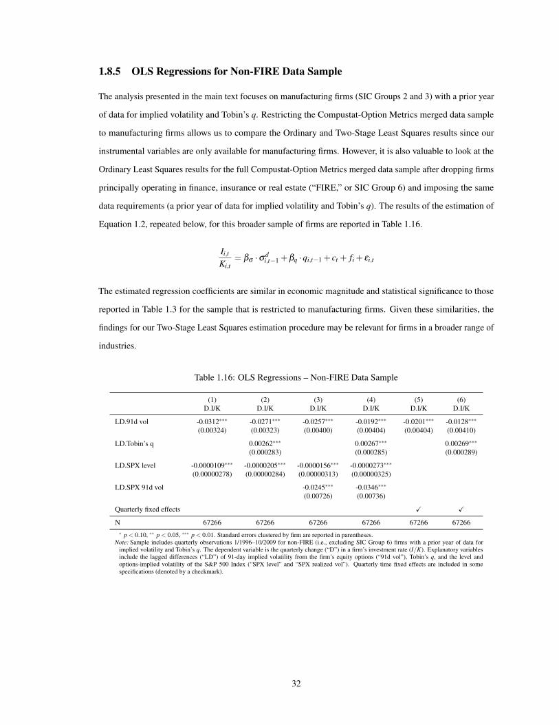
1.8.5 OLS Regressions for Non-FIRE Data Sample

The analysis presented in the main text focuses on manufacturing firms (SIC Groups 2 and 3) with a prior year

of data for implied volatility and Tobin’s q. Restricting the Compustat-Option Metrics merged data sample

to manufacturing firms allows us to compare the Ordinary and Two-Stage Least Squares results since our

instrumental variables are only available for manufacturing firms. However, it is also valuable to look at the

Ordinary Least Squares results for the full Compustat-Option Metrics merged data sample after dropping firms

principally operating in finance, insurance or real estate (“FIRE,” or SIC Group 6) and imposing the same

data requirements (a prior year of data for implied volatility and Tobin’s q). The results of the estimation of

Equation 1.2, repeated below, for this broader sample of firms are reported in Table 1.16.

Ii,t

Ki,t= βσ ·σd

i,t−1 +βq ·qi,t−1 + ct + fi + εi,t

The estimated regression coefficients are similar in economic magnitude and statistical significance to those

reported in Table 1.3 for the sample that is restricted to manufacturing firms. Given these similarities, the

findings for our Two-Stage Least Squares estimation procedure may be relevant for firms in a broader range of

industries.

Table 1.16: OLS Regressions – Non-FIRE Data Sample

(1) (2) (3) (4) (5) (6)D.I/K D.I/K D.I/K D.I/K D.I/K D.I/K

LD.91d vol -0.0312∗∗∗ -0.0271∗∗∗ -0.0257∗∗∗ -0.0192∗∗∗ -0.0201∗∗∗ -0.0128∗∗∗

(0.00324) (0.00323) (0.00400) (0.00404) (0.00404) (0.00410)

LD.Tobin’s q 0.00262∗∗∗ 0.00267∗∗∗ 0.00269∗∗∗

(0.000283) (0.000285) (0.000289)

LD.SPX level -0.0000109∗∗∗ -0.0000205∗∗∗ -0.0000156∗∗∗ -0.0000273∗∗∗

(0.00000278) (0.00000284) (0.00000313) (0.00000325)

LD.SPX 91d vol -0.0245∗∗∗ -0.0346∗∗∗

(0.00726) (0.00736)

Quarterly fixed effects X X

N 67266 67266 67266 67266 67266 67266∗ p < 0.10, ∗∗ p < 0.05, ∗∗∗ p < 0.01. Standard errors clustered by firm are reported in parentheses.

Note: Sample includes quarterly observations 1/1996–10/2009 for non-FIRE (i.e., excluding SIC Group 6) firms with a prior year of data forimplied volatility and Tobin’s q. The dependent variable is the quarterly change (“D”) in a firm’s investment rate (I/K). Explanatory variablesinclude the lagged differences (“LD”) of 91-day implied volatility from the firm’s equity options (“91d vol”), Tobin’s q, and the level andoptions-implied volatility of the S&P 500 Index (“SPX level” and “SPX realized vol”). Quarterly time fixed effects are included in somespecifications (denoted by a checkmark).

32

1.8.6 Results Using Realized Volatility Measure

Table 1.17: Relevant Timing – Realized Volatility

(1) (2) (3) (4) (5) (6)D.I/K D.I/K D.I/K D.I/K D.I/K D.I/K

D.Realized vol -0.00101 -0.00514∗

(0.00269) (0.00277)

LD.Realized vol -0.00823∗∗∗ -0.0116∗∗∗

(0.00296) (0.00282)

L2D.Realized vol -0.00461 -0.00916∗∗∗

(0.00299) (0.00295)

L3D.Realized vol 0.000468 -0.00451(0.00315) (0.00291)

L4D.Realized vol -0.00121 -0.00349(0.00332) (0.00336)

LD.SPX level -0.00000489 -0.00000661∗ -0.00000472 -0.00000451 -0.00000467 -0.0000103∗∗∗

(0.00000347) (0.00000359) (0.00000340) (0.00000340) (0.00000344) (0.00000372)

N 35835 35835 35835 35835 35835 35835∗ p < 0.10, ∗∗ p < 0.05, ∗∗∗ p < 0.01. Standard errors clustered by firm are reported in parentheses.

Note: Sample includes quarterly observations 1/1996–10/2009 for manufacturing (SIC Groups 2 and 3) firms with a prior year of data forimplied volatility and Tobin’s q. The dependent variable is the quarterly change (“D”) in a firm’s investment rate (I/K). Explanatory variablesinclude the quarterly change (“D”) in the average realized volatility of the firm’s stock price (“Realized vol”) and level of the S&P 500 Index(“SPX level”). Specifications vary in the length of lag at which we consider the change in realized volatility, ranging from contemporary(“D”) to a four-quarter lag (“L4D”).

Table 1.18: OLS Regressions – Implied and Realized Volatility

(1) (2) (3) (4) (5) (6)D.I/K D.I/K D.I/K D.I/K D.I/K D.I/K

LD.91d vol -0.0283∗∗∗ -0.0229∗∗∗ -0.0231∗∗∗ -0.0161∗∗ -0.0222∗∗∗ -0.0149∗∗

(0.00634) (0.00640) (0.00697) (0.00712) (0.00709) (0.00725)

LD.Realized vol 0.000135 -0.00137 0.00589 0.00496 0.00505 0.00436(0.00366) (0.00363) (0.00373) (0.00369) (0.00374) (0.00372)

LD.Tobin’s q 0.00234∗∗∗ 0.00244∗∗∗ 0.00236∗∗∗

(0.000360) (0.000363) (0.000364)

LD.SPX level -0.0000117∗∗∗ -0.0000212∗∗∗ -0.00000773∗∗ -0.0000185∗∗∗

(0.00000370) (0.00000369) (0.00000393) (0.00000401)

LD.SPX 91d vol 0.101∗∗∗ 0.102∗∗∗

(0.0221) (0.0222)

LD.SPX realized vol -0.0845∗∗∗ -0.0904∗∗∗

(0.0139) (0.0140)

Quarterly fixed effects X X

N 35835 35835 35835 35835 35835 35835∗ p < 0.10, ∗∗ p < 0.05, ∗∗∗ p < 0.01. Standard errors clustered by firm are reported in parentheses.

Note: Sample includes quarterly observations 1/1996–10/2009 for manufacturing (SIC Groups 2 and 3) firms with a prior year of data for impliedvolatility, realized volatility, and Tobin’s q. The dependent variable is the quarterly change (“D”) in a firm’s investment rate (I/K). Explanatoryvariables include the lagged differences (“LD”) of 91-day implied volatility from the firm’s equity options (“91d vol”), average realized volatilityof the firm’s stock price (“Realized vol”), Tobin’s q, and the level, 91-day implied volatility, and realized volatility of the S&P 500 Index (“SPXlevel”, “SPX 91d vol”, and “SPX realized vol”). Quarterly time fixed effects are included in some specifications (denoted by a checkmark).

33

Table 1.19: Two-Stage Least Squares Estimation – Realized Volatility

(1) (2) (3) (4) (5) (6)D.I/K D.I/K D.I/K D.I/K D.I/K D.I/K

LD.Realized vol -0.0404∗∗∗ -0.0554∗∗∗ -0.0542∗∗∗ -0.0769∗∗∗ 0.00781 -0.00433(0.00571) (0.00655) (0.0158) (0.0174) (0.0188) (0.0149)

LD.Tobin’s q 0.0166∗∗∗ 0.0169∗∗∗ 0.00252(0.00482) (0.00491) (0.00347)

LD.SPX level -0.0000149∗∗∗ -0.0000935∗∗∗ -0.0000145∗∗∗ -0.0000923∗∗∗

(0.00000374) (0.0000228) (0.00000379) (0.0000230)

LD.SPX realized vol 0.0140 0.0282(0.0169) (0.0182)

Quarterly fixed effects X X

N 35835 35835 35835 35835 35835 35835∗ p < 0.10, ∗∗ p < 0.05, ∗∗∗ p < 0.01. Standard errors clustered by firm are reported in parentheses.

Note: Sample includes quarterly observations 1/1996–10/2009 for manufacturing (SIC Groups 2 and 3) firms with a prior year of data forimplied volatility, realized volatility, and Tobin’s q. The dependent variable is the quarterly change (“D”) in a firm’s investment rate (I/K).Explanatory variables include the lagged differences (“LD”) of average realized volatility of the firm’s stock price (“Realized vol”), Tobin’sq, and the level and average realized volatility of the S&P 500 Index (“‘SPX level” and ‘SPX realized vol”). Firm-specific realized volatilityand Tobin’s q are instrumented using exposure to energy and currency volatility and prices. Quarterly time fixed effects are included insome specifications (denoted by a checkmark).

1.8.7 Relationship Between Implied Volatility and Tobin’s q

Kogan (2004) discusses the empirical implications of a general equilibrium model in which both investment

and the volatility of asset prices are endogenous (Kogan, 2001). In response to a shock to the state of the

economy, firms adjust their capital stocks as long as they are not constrained by investment irreversibilities or

upper bounds on the investment rate. If they are constrained, asset prices absorb the shock, thereby producing

greater volatility. The model uses Tobin’s q as a sufficient statistic for the state of the economy and predicts

a non-linear relationship between Tobin’s q and stock price volatility. Following Kogan’s theory, we look

at the relationship between our firm-level measure of implied volatility and Tobin’s q. Consistent with his

predictions, we find evidence of a non-linear relationship. The results are reported in Table 1.20.

34

Table 1.20: Relationship between Implied Volatility and Tobin’s q

(1) (2) (3) (4)91d vol 91d vol D.91d vol D.91d vol

Tobin’s q 0.00920∗∗∗ -0.00984∗∗∗

(0.000700) (0.00252)

Tobin’s q squared 0.000982∗∗∗

(0.000121)

D.Tobin’s q -0.00870∗∗∗ -0.0245∗∗∗

(0.000433) (0.00122)

D.Tobin’s q squared 0.000716∗∗∗

(0.0000507)

N 35835 35835 35835 35835∗ p < 0.10, ∗∗ p < 0.05, ∗∗∗ p < 0.01. Standard errors clustered by firm are reported in paren-theses.

Note: Sample includes quarterly observations 1/1996–10/2009 for manufacturing (SIC Groups 2and 3) firms with a prior year of data for implied volatility and Tobin’s q. In columns (1)–(2),the dependent variable is the 91-day implied volatility from a firm’s equity options (“91d vol”)and explanatory variables are functions of the firm’s Tobin’s q. Columns (3)–(4) are similar, butconsider the quarterly change (“D”) in these variables.

35

Bibliography

Abel, A. B. Optimal investment under uncertainty. American Economic Review, 73, 228–233, 1983.

Abel, A. B. and J. Eberly. A unified model of investment under uncertainty. American Economic Review,84(5), 1369–1384, 1994.

Aivazian, V. A., Y. Geb, and J. Qiu. The impact of leverage on firm investment: Canadian evidence. Journalof Corporate Finance, 11(1-2), 277–291, 2005.

Arellano, M. and S. Bond. Some tests of specification for panel data: Monte Carlo evidence and an applicationto employment equations. Review of Economic Studies, 58(2), 277–297, 1991.

Bachmann, R., S. Elstner, and E. Sims. Uncertainty and economic activity: Evidence from business surveydata. Working Paper, 2010.

Baum, C. F., M. Caglayan, and O. Talavera. Uncertainty determinants of firm investment. Working Paper,2007.

Bernanke, B. S. Irreversibility, uncertainty and cyclical investment. Quarterly Journal of Economics, 98,85–106, 1983.

Bloom, N. The impact of uncertainty shocks. Econometrica, 77, 623–685, 2009.

Bloom, N., S. Bond, and J. Van Reenen. Uncertainty and investment dynamics. Review of Economic Studies,74(2), 391–415, 2007.

Bloom, N., M. Floetotto, and N. Jaimovich. Really uncertain business cycles. Working Paper, 2009.

Blundell, R. and S. Bond. Initial conditions and moment restrictions in dynamic panel data models. Journal ofEconometrics, 87(1), 115–143, 1998.

Blundell, R., S. Bond, M. Devereux, and F. Schiantarelli. Investment and Tobin’s Q: Evidence from companypanel data. Journal of Econometrics, 51(1-2), 233–257, 1992.

Bond, S., R. Moessner, H. Mumtaz, and M. Syed. Microeconometric evidence on uncertainty and investment.Technical report, mimeo, Institute for Fiscal Studies, London, 2005.

Brunnermeier, M. K. and Y. Sannikov. A macroeconomic model with a financial sector. Working Paper, 2009.

Caballero, R. J. On the sign of the investment-uncertainty relationship. Review of Economic Studies, 81,278–288, 1991.

Campa, J. M. Entry by foreign firms in the United States under exchange rate uncertainty. Review of Economicsand Statistics, 75, 614–622, 1993.

Campa, J. M. and L. S. Goldberg. Investment in manufacturing, exchange rates and external exposure. Journalof International Economics, 38, 297–320, 1993.

Carruth, A., A. Dickerson, and A. Henley. What do we know about investment under uncertainty? Journal ofEconomic Surveys, 14(2), 119–154, 2000.

36

Christensen, B. and N. Prabhala. The relation between implied and realized volatility. Journal of FinancialEconomics, 50(2), 125–150, 1998.

Chung, K. and S. Pruitt. A simple approximation of Tobin’s Q. Financial Management, 23, 70–74, 1994.

Cummins, J., K. Hassett, and S. Oliner. Investment behavior, observable expectations, and internal funds.American Economic Review, 96(3), 796–810, 2006.

Davis, S. J. and J. Haltiwanger. Gross job creation, gross job destruction, and employment reallocation.Quarterly Journal of Economics, 107, 819–863, 1992.

Dixit, A. Investment and hysteresis. Journal of Economic Perspectives, 6(1), 107–132, 1992.

Dixit, A. and R. Pindyck. Investment Under Uncertainty. Princeton University Press, 1994.

Ferderer, P. J. The impact of uncertainty on aggregate investment spending: An empirical analysis. Journal ofMoney, Credit and Banking, 25, 30–48, 1993.

Ghosal, V. and P. Loungani. Product market competition and the impact of price uncertainty on investment:Some evidence from U.S. manufacturing industries. Journal of Industrial Economics, 217–228, 1996.

Goldberg, L. S. Exchange rates and investment in United States industry. Review of Economics and Statistics,75, 575–589, 1993.

Guay, W. and S. Kothari. How much do firms hedge with derivatives? Journal of Financial Economics, 70(3),423–461, 2003.

Guiso, L. and G. Parigi. Investment and demand uncertainty. Quarterly Journal of Economics, 114(1),185–227, 1999.

Hall, R. Investment, interest rates, and the effects of stabilization policies. Brookings Papers on EconomicActivity, 1, 61–121, 1977.

Hartman, R. The effects of price and cost uncertainty on investment. Journal of Economic Theory, 5, 258–266,1972.

Hayashi, F. Tobin’s marginal q and average q: A neoclassical interpretation. Econometrica, 50, 213–224,1982.

Huizinga, J. Inflation uncertainty, relative price uncertainty, and investment in U.S. manufacturing. Journal ofMoney, Credit & Banking, 25, 521–554, 1993.

Ingersoll, J. and S. A. Ross. Waiting to invest: Investment and uncertainty. Journal of Business, 65, 1–29,1992.

Julio, B. and Y. Yook. Political uncertainty and corporate investment cycles. Working Paper, 2009.

Kogan, L. An equilibrium model of irreversible investment. Journal of Financial Economics, 62, 201–245,2001.

Kogan, L. Asset prices and real investment. Journal of Financial Economics, 73, 411–431, 2004.

Leahy, J. V. and T. M. Whited. The effect of uncertainty on investment: Some stylized facts. Journal of Money,Credit and Banking, 28(1), 64–83, 1996.

Lee, J. and K. Shin. The role of a variable input in the relationship between investment and uncertainty.American Economic Review, 667–680, 2000.

Pindyck, R. A note on competitive investment under uncertainty. American Economic Review, 273–277, 1993.

Pindyck, R. S. Capital risk and models of investment behaviour. Technical report, mimeo, Sloan School ofManagement, MIT, 1986.

37

Pindyck, R. S. Irreversible investment, capacity choice, and the value of the firm. American Economic Review,83, 273–277, 1988.

Pindyck, R. S. Irreversibility, uncertainty, and investment. Journal of Economic Literature, 29(3), 1110–1148,1991.

Price, S. Aggregate uncertainty, capacity utilization and manufacturing investment. Applied Economics, 27,147–154, 1995.

Price, S. Aggregate uncertainty, investment and asymmetric adjustment in the U.K. manufacturing sector.Applied Economics, 28, 1369–1379, 1996.

Rajan, R. and L. Zingales. Financial dependence and growth. American Economic Review, 88, 559–586, 1998.

Ratti, R. and K. H. Yoon. Energy price uncertainty, energy intensity and firm investment. Working Paper,2009.

Salinger, M. and L. Summers. Tax reform and corporate investment: A microeconometric simulation study.In M. Feldstein, editor, Behavioral Simulation Methods in Tax Policy Analysis, 247–287. University ofChicago Press, 1983.

Schwert, G. W. Stock volatility in the new millennium: How wacky is Nasdaq? Journal of MonetaryEconomics, 49, 3–26, 2002.

Shiller, R. Market Volatility. The MIT Press, 1992.

Stock, J. H. and M. Yogo. Testing for Weak Instruments in Linear IV Regression. Cambridge University Press,2005.

38

Chapter 2

Regulated Technology Diffusion: The SEC and the Impact of PennyPricing in Electronic Options Trading

2.1 Introduction

Innovation has long been a fundamental driver of financial market development. In recent years, prominent

areas of innovation have included both the development of new products, such as derivatives and mortgage-

backed securities, as well as the development of new technologies, such as trading algorithms and electronic

market infrastructure. The widespread distress experienced by financial companies over the past two years has

generated scepticism regarding the value of financial innovation and the effectiveness of regulatory agencies.

Nevertheless, electronic trading innovations have been a primary source of market advancement over the past

decade and regulation by the Securities Exchange Commission (SEC) has played a central role in shaping this

progress.

While the emergence of electronic trading technology applies to an array of recent developments, innovation

in the equity options market presents a particularly interesting case study. In February 2007, the SEC

implemented the first phase of a “penny pricing" trial in the exchange-traded options market.1 The initial

phase of this trial required the six United States options exchanges to reduce the minimum bid-offer spread

from five or ten cents to a penny for the options corresponding to thirteen underlying equity securities.2 The

catalyst for this pricing change was the improved electronic capabilities of the exchanges. Over the course

of the preceding decade, the exchanges invested in the development of systems that would allow them to

offer electronic trading in addition to traditional open-outcry trading. Instead of picking up the telephone and

calling a broker or market maker on the trading floor, customers could simply look at the bid-offer quotes and

1The authority implicit in the SEC’s mandate was established by the Securities Exchange Act of 1934, which gave the SEC theresponsibility to regulate the trading of securities in the secondary markets.

2The six United States options exchanges are the Chicago Board Options Exchange (CBOE), the International Securities Exchange(ISE), the New York Stock Exchange Arca (NYSE Arca), the Philadelphia Stock Exchange (PHLX), the American Stock Exchange(AMEX) and the Boston Options Exchange (BOX). In March 2008, Nasdaq Options Market entered as the seventh U.S. options exchange.Specifically, the minimum bid-offer spread for pilot options series was reduced from $0.05 to $0.01 for options trading below $3 and wasreduced from $0.10 to $0.05 for options trading at or above $3. The QQQQ options series are the exception: for the pilot, all QQQQoptions must be quoted using $0.01 minimum bid-offer spreads regardless of the price level.

39

available volumes on their computer screens and execute trades directly through these electronic platforms.

With the transition to electronic trading platforms came the capability to disseminate price quotes and

execute trades with much greater speed, data capacity, and interconnectedness among exchanges. Rather

than being limited by the human capabilities underlying the open-outcry technology, computers offered the

potential for superior performance, especially during periods of high market volatility and trading volume. In

its oversight role, the SEC was aware of the exchanges’ new electronic capabilities and saw an opportunity to

put these capabilities to full use. Considering the exchanges’ ability to post and adjust quotes more efficiently,

the existing five and ten-cent bid-offer spreads seemed artificially wide, potentially generating excessive

rents for market makers. Instead, it seemed feasible for options to be quoted and traded in penny increments,

resulting in improved prices for investors.

Effectively, this narrower bid-offer spread redistributes the gains of innovation from the exchanges’ market

makers to investors. The reduced transaction costs and greater price transparency associated with penny

bid-offer spreads represent a reduction of market frictions for investors. On the other hand, wider bid-offer

spreads may be optimal to induce market makers to provide liquidity despite inventory costs and information

asymmetries relative to informed traders (see Glosten and Milgrom, 1985). Of course, if the pricing change

leads to a substantial increase in trading volume, market makers may ultimately benefit despite the narrower

spreads.

An interesting aspect of the pricing change has been the mixed reaction among exchanges and investor

groups. While a decreased bid-offer spread would seem to be a movement toward greater price transparency

and market efficiency, several market participants have been critical of the change, claiming it has been

disruptive to the market. Some exchanges have met with success, while others have pointed to significant

declines in volume and liquidity.3 This paper’s central objective is to investigate the ways in which electronic

trading innovations, and penny pricing in particular, are impacting the market. A critical step in pursuing this

objective is to independently analyze market data and assess whether the views advocated by the SEC and the

exchanges are consistent with the story told by the data. A closely related objective is to identify the pilot’s

repercussions for the option market’s structure and evaluate whether these developments potentially interfere

with the SEC’s stated mission of improving individual investors’ welfare.

In the following sections of the paper I address these considerations in detail. I begin with a background

discussion of technology development in the options market and the SEC’s implementation of the Penny Pilot

in response to these improvements. Section 2.3 presents a detailed analysis of the impact of the pricing change

on various market liquidity measures. The results include strong evidence of narrower bid-offer spreads,

3In particular, NYSE Arca and BOX have submitted reports strongly in favor of penny pricing while CBOE, ISE and PHLX haveencouraged caution in the pilot’s expansion.

40

thinner quote markets, and economically insignificant changes in trading volume. This is followed by a

discussion of some of the unexpected repercussions of the pricing change and their relationship to the SEC’s

stated objectives. I conclude by highlighting the exchanges’ incentives for further innovation, many of which

are a direct result of the pricing change.

2.2 Implementation of the Penny Pilot

Electronic communication networks (ECNs) were first authorized by the SEC in 1998 to facilitate trading of

financial products outside of physical exchanges. While ECNs were introduced to the equity market at that

time, they did not appear in the options market until the International Securities Exchange (ISE) introduced

the United States’ first fully electronic options trading platform in May 2000. Rather than calling a broker or

exchange market maker, ISE’s customers were able to view price and quantity quotes for option securities

on their computer screens and execute trades directly through the computer interface. ISE’s introduction of

electronic trading to the options market induced an industry-wide wave of competitive innovation. By 2005,

the five other options exchanges had all introduced electronic trading capabilities to operate in tandem with

their trading floors.

The technology underlying electronic trading platforms allowed the exchanges’ market makers to post,

broadcast, and adjust price quotes more efficiently. These capabilities led the SEC to question whether the

existing five and ten-cent minimum bid-offer spreads were artificially wide, potentially generating excessive

rents for market makers.4 The SEC found that for the most actively traded options, the national best bid-offer

spread was at the minimum increment for more than 50 percent of the trading day. This statistic signalled

that the existing minimum quote increments were binding constraints and that, if facilitated, greater price

competition among market makers might result in narrower spreads and improved prices for investors.

Rather than immediately transitioning all options to penny spreads, the SEC took a measured approach

and instituted a multiple phase trial process. The Penny Pilot began in February 2007 and required the six

United States options exchanges to reduce the minimum bid-offer spread from five or ten cents to a penny for

the options corresponding to thirteen underlying equity securities. Beginning in September 2007, the second

phase introduced an additional 22 names to the trial group. This continued until March 2008, when the SEC

added another 28 names.

Regarding the selection of the pilot securities, the SEC’s January 2007 announcement described the Phase 1

securities as a diverse group of options with a variety of trading characteristics. The SEC intended to use

information from the pilot securities to assess the likely impact of a broader pricing change on bid-offer

4The recent explosion of options trading volume likely drew attention to these market maker profits and their potential excess.

41

spreads, market liquidity, and quote traffic. However, looking closely at the Phase 1 securities, they are options

on well-known companies with substantial trading volume and are primarily drawn from a limited subset of

industries.5 This calls into question whether the pilot series are truly a representative sample. Rather, the

SEC may have given the penny pricing trial the best possible chance to succeed by selecting options that are

relatively easy to trade in terms of liquidity.

In encouraging the option market’s transition to penny pricing, the SEC heavily relied on the positive

experiences of the equity market following “decimalization" in 2001. As a result, the SEC expected penny

pricing to achieve narrower bid-offer spreads, increases in trading volume, and overall improvements in

liquidity and price transparency. A number of scholarly papers investigate the equity market’s transition to

penny bid-offer spreads (for example, see Bessembinder (2003), Chakravarty, Wood and Van Ness (2004), and

Gibson, Singh and Yeramilli (2003)). One of the central contributions of this paper is to highlight differences in

the impact of penny pricing in the options market versus the equity market that are attributable to fundamental

differences in the markets’ characteristics. For example, a unique feature of the options market is the existence

of a thriving over-the-counter (OTC) market. The OTC market provides an alternative trading venue for

institutional customers frustrated by the decline in market depth at the exchanges. This potential movement

away from the exchanges may explain the observation that trading volume has not increased in response to the

narrower bid-offer spreads, in contrast to the increases in activity experienced by the equity market.

In the following sections of the paper, I present an analysis of the impact of penny pricing on a variety

of liquidity measures and discuss ways in which the regulatory change has influenced market structure and

trading dynamics. In light of the various market repercussions, has the pilot achieved the SEC’s goal of

improving investor welfare? As some market participants argue, have the gains been achieved at the expense

of market liquidity? How have exchanges and investors responded to the new regulation? In particular, how

has trading behavior changed and what incentives are there for further technological progress?

2.3 Market Impact

Potentially distinct from the SEC’s objectives is the observed impact of its regulatory actions. A central

research objective is to investigate the ways in which penny pricing is affecting option market trading dynamics.

The first step in addressing this objective is to analyze options trading data and evaluate the effect of the pilot

on market liquidity.

In order to address this question, I first need to define “liquidity" and determine an appropriate measure. I

consider liquidity in a broad sense as the “ease of trading" a given security and attempt to quantify the impact

5The majority of the Phase 1 pilot series come from the computer hardware, semiconductor, and related industries. Phases 2 and 3 of thepilot introduce options series from the financial, energy, automotive and retail industries.

42

of the pricing change on a variety of market variables jointly relevant as measures of liquidity. The pilot is

essentially an exogenous shock to bid-offer spreads, which are often cited as a proxy for market liquidity

constraints since they measure direct transaction costs. Bid-offer spreads are certainly not a perfect measure

since they do not reflect the available trading size at a given price. For this reason, considering variables such

as bid and offer quote sizes, trading volume, average transaction size, and the number of market maker price

quotes helps to paint a more comprehensive picture of market liquidity. The pilot likely affected all of these

market variables to some extent. Therefore, an evaluation of the pilot’s impact should address this combination

of factors.6

While a formal model of market microstructure is beyond the scope of this paper, it is useful to discuss

some hypotheses regarding the potential market reaction to penny pricing. The first perspective views this

change in the context of a standard supply and demand argument. A reduction in the minimum bid-offer

spread reduces investors’ transaction costs, thereby lowering the price of trading. In response to a lower price,

we might expect a higher demand for options trading which would lead to an increase in trading volume. This

scenario underlies the SEC’s optimistic expectations for penny pricing.

The second perspective draws from Glosten and Milgrom’s (1985) model of a securities market in which

there is asymmetric information. In this model, market participants include informed traders, uninformed

liquidity traders, and market makers who are uninformed but gradually incorporate market information into

their bid and offer prices.7 In this setting, the bid-offer spread serves as a buffer for the market maker’s

incomplete information regarding the security’s true value. As a result, a greater degree of information

asymmetry leads to a wider bid-offer spread.

Applying this concept to the Penny Pilot, a narrower bid-offer spread may reduce a market maker’s

willingness to provide price quotes because the spread does not sufficiently compensate him for the risks

associated with asymmetric information relative to informed traders. More generally, a reduced bid-offer

spread lowers the profits available to a market maker relative to any sort of cost, whether it be information

risks or overhead and inventory costs.8 If market makers have less of an incentive to provide liquidity, the

market may experience declines in bid and offer quote sizes or a contraction of quotes to some subset of the

original menu of available securities. As a result, the market may attract less customer trading volume.9

6Rather than suggesting a formal weighting of the various factors, my definition of liquidity as the “ease of trading" a security providesmore flexibility. In my analysis, I assess the economical and statistical impact of the pilot on each of the liquidity factors and then drawconclusions based on a general synthesis of the findings.

7The characterization of being “informed" means that a participant knows the true value of the security. In setting bid and offer prices, amarket maker takes into account the information he has gathered about the security’s value from previous trades and also incorporatesthe additional information he will gain when a trader wishes to either buy or sell a given security.

8In Glosten and Milgrom (1985), trades are limited to a single unit of the security. In reality, trades occur at a wide range of possiblequantities. Therefore, a market maker can provide less liquidity by reducing the quantity he is willing to trade at a given price.

9It is important to emphasize that the pilot does not require market makers to reduce the size of their bid-offer spreads. Rather, the pilotencourages market makers to engage in price competition by reducing their bid-offer spreads below the previous minimum of five cents.To the extent that there is variation in market makers’ information or overhead costs, there may be variation in the minimum spread at

43

These theories provide a framework which guides the analysis performed in the following sections of

the paper. In particular, they suggest possible responses to the pilot. We may observe increased customer

demand and trading volume due to lower transaction costs, decreased supply of liquidity due to market makers’

reduced incentives, or some combination of the two across different types of securities. Given this framework,

I investigate the impact of the pilot on market liquidity from several perspectives. The first strategy tests for

significant changes in trading variables such as bid-offer spreads, volume, and quote sizes that are attributable

to the pilot implementation. This requires a before and after analysis that controls for contemporaneous market

dynamics. In addition, I estimate a probit model to evaluate whether the pilot has affected the probability that a

security trades on a particular day. In all of these analyses, I allow the impact of the pilot to differ for different

types of options securities. For example, the response of options with equity underlyings may differ from that

of options with index underlyings due to fundamental differences in the trading dynamics of the two groups.

Another segment of the analysis introduces the possibility that despite the discrete start of Phase 1 of

the pilot on February 9, 2007, the market’s adjustment to penny pricing may be more of a gradual and

continuous transition. Perhaps market makers will not immediately reduce bid-offer spreads to the new

minimum increments, but rather will gradually reduce them over time as they adjust to the new pricing,

quoting, and trading processes. Similarly, bid and offer quote sizes may have been drastically cut in the early

days of the pilot, but then recovered over time. Evidence of a gradual transition process would signal that a

short-horizon analysis is insufficient to fully identify the impact of the pricing change.

2.3.1 Data

The gradual implementation of penny pricing presents an ideal experimental setting for economic analysis.

Defining control groups using options series that were not included in the pilot, the options series included in

the various phases are the treatment groups. In order to identify the impact of the pricing change, I rely upon

detailed trading data on the pilot options series as well as data on a group of comparable securities and control

variables for overall market volatility and trading activity. This data is archived by the Options Price Reporting

Authority (OPRA), the data feed that collects details on option quotes and trades across all of the exchanges.

Given the well-documented challenges associated with intra-day tick data, I focus my analysis on summary

information derived from the OPRA tick data.10 While tick data contains a wealth of valuable information,

performing the analysis at a daily frequency permits a preliminary evaluation of variables fundamentally

which they are willing to trade or variation in the quantity they are willing to trade at a given price.10Tick data presents challenges including widespread reporting errors and the treatment of time when the data is asynchronous and the

frequency of market activity differs across securities and times of day. The summary data used in my analysis is generated by theChicago Board Options Exchange research group using the filtered archive of OPRA tick data that they maintain.

44

relevant to the broad impact of penny pricing on options market liquidity.11

The data set includes daily observations from August 2006 through August 2007, allowing me to analyze

trading patterns before and after the start of the pilot in February 2007. This time period isolates the impact

of the first phase alone since the second phase did not begin until September 2007. The panel of securities

includes the thirteen Phase 1 series as well as a selection of comparable securities to use as controls. A list of

these securities is provided in Table 2.1. The comparables were selected according to five dimensions: (1)

industry membership for equity series and index nature for the index series (i.e. broad market or sector-specific

index); (2) equity market capitalization; (3) equity trading volume; (4) options trading volume; and (5) options

open interest.12 The goal of this approach is to select comparables with trading and liquidity properties similar

to those of the pilot series before the implementation of the pilot. Additional details on the control selection

process are provided in the Appendix.

For each equity underlying, I have daily data for all of the corresponding options series broken down

according to expiration date and strike price. This data includes the following variables: trading volume,

number of quotes, average transaction size, average bid-offer spread, and average inside (“best") bid and offer

quote sizes. It is important to emphasize that the observations for bid-offer spreads and quote sizes are average

values across the full trading day. They are not simply values observed at market close. In addition, I use daily

data from the Chicago Board Options Exchange (CBOE) on total options trading volume, the level of the

S&P 500 Volatility Index (VIX), and the return on the S&P 500 Index in order to control for broad market

dynamics.

Table 2.1: Phase 1 and Comparable Securities

Phase 1 Securities Comparable SecuritiesA Agilent Tech JBL Jabil CircuitAMD Advanced Micro Devices NVDA NVIDIA CorporationCAT Caterpillar DE Deere & CompanyFLEX Flextronics International AMKR Amkor TechnologyGE General Electric UTX United TechnologiesINTC Intel MU Micron TechnologyIWM Ishares Russell 2000 DIA Diamonds TrustMSFT Microsoft AAPL Apple ComputersQQQQ Nasdaq Powershares SPY SPDR TrustSMH SemiConductor Holders OIH Oil Service HoldersSUNW Sun Micro HPQ Hewlett-PackardTXN Texas Instruments ADI Analog DevicesWFMI Whole Foods SWY Safeway

11Future work with tick data will be valuable in addressing a variety of questions the daily data cannot (i.e., price and quote dynamics,quote submission strategies, and intraday liquidity patterns).

12Open interest is the number of outstanding exchange-traded options contracts and is therefore an alternative measure of trading activity.

45

2.3.2 Descriptive Statistics

To provide a preliminary sense of the data, I calculate and report a variety of descriptive statistics. In looking

at these statistics for the full data set, there are some outlier observations. For example, there are observations

with negative values for trading volume or unreasonably large values for volume, bid size or offer size. In

addition, there are observations with extreme values for bid-offer spreads, some in the thousands of dollars and

others less than the exchange mandated minimum increments. Given the scope and detail of the OPRA data,

the presence of occasional reporting errors is not surprising. As a precaution against using these inaccurate

data feeds in the analysis, I exclude observations falling below the 1st percentile or above the 99th percentile

for any of the variables of interest. For the average bid-offer spread variable, I drop any observations less than

the minimum increment ($0.05 pre-pilot and $0.01 post-pilot) or above the 99th percentile value of $0.86. The

total number of remaining observations is 9,660,993. Each of these observations is daily data for an option

series with a particular strike and expiration date corresponding to one of the equity underlyings.

The descriptive statistics reported in Tables 2.2-2.5 include means, medians and standard deviations for the

variables of interest. In addition to statistics for the full sample, I include separate statistics for the pilot series,

the pilot series excluding those with index underlyings, and the control sample. It seems plausible that options

corresponding to index versus equity underlyings may respond differently to a narrower minimum bid-offer

spread. In particular, if index options are more liquid, the previous five and ten-cent minimum bid-offer spreads

may have been more restrictive constraints.

Due to the predominance of observations with zero trading volume, I also report descriptive statistics for a

sample restricted to observations with positive volume. Most of the zero volume observations correspond to far

out-of-the-money options or longer-dated LEAP (Long Term Equity AnticiPation Security) options. A potential

concern arises in using observations of bid-offer spreads or bid and offer quote sizes if the corresponding

option did not actually trade on that date. To some extent, positive trading volume corroborates the reliability

of the data for the other variables. Excluding the observations with zero trading volume drastically reduces the

number of observations to 1,467,151. For robustness, the analyses presented throughout the paper have been

repeated both including and excluding observations with zero trading volume. I also explicitly consider the

effect of the pilot on the probability of positive trading volume in Section 2.3.4.

The statistics in Tables 2.2-2.5 illustrate a variety of patterns. The mean and median trading volume

and average transaction size increased for all four of the security groups, except for a decline in the mean

transaction size for pilot series with equity rather than index underlyings. The largest increases often occurred

for the pilot series. Similarly, the number of quotes increased across the board, with a substantial jump in the

mean for the pilot series from 1915 to 3869 quotes per day. As expected, the average bid-offer spread fell for

46

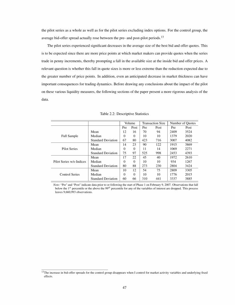
the pilot series as a whole as well as for the pilot series excluding index options. For the control group, the

average bid-offer spread actually rose between the pre- and post-pilot periods.13

The pilot series experienced significant decreases in the average size of the best bid and offer quotes. This

is to be expected since there are more price points at which market makers can provide quotes when the series

trade in penny increments, thereby prompting a fall in the available size at the inside bid and offer prices. A

relevant question is whether this fall in quote sizes is more or less extreme than the reduction expected due to

the greater number of price points. In addition, even an anticipated decrease in market thickness can have

important consequences for trading dynamics. Before drawing any conclusions about the impact of the pilot

on these various liquidity measures, the following sections of the paper present a more rigorous analysis of the

data.

Table 2.2: Descriptive Statistics

Volume Transaction Size Number of QuotesPre Post Pre Post Pre Post

Full SampleMean 12 16 70 94 2409 3524Median 0 0 10 10 1379 2020Standard Deviation 67 80 423 716 3007 4082

Pilot SeriesMean 14 23 90 122 1915 3869Median 0 0 11 14 1069 2271Standard Deviation 75 97 525 998 2453 4393

Pilot Series w/o IndicesMean 17 22 45 40 1972 2610Median 0 0 10 10 934 1267Standard Deviation 80 88 273 230 2804 3424

Control SeriesMean 10 12 54 75 2809 3305Median 0 0 10 10 1776 2015Standard Deviation 60 66 310 441 3337 3885

Note: “Pre" and “Post" indicate data prior to or following the start of Phase 1 on February 9, 2007. Observations that fallbelow the 1st percentile or the above the 99th percentile for any of the variables of interest are dropped. This processleaves 9,660,993 observations.

13The increase in bid-offer spreads for the control group disappears when I control for market activity variables and underlying fixedeffects.

47

Table 2.3: Descriptive Statistics

Bid-Offer Spread Bid Size Ask SizePre Post Pre Post Pre Post

Full SampleMean 0.17 0.18 1217 906 1674 1143Median 0.16 0.14 307 275 540 369Standard Deviation 0.11 0.15 2202 1665 2744 2012

Pilot SeriesMean 0.16 0.11 1268 606 1764 747Median 0.15 0.08 355 256 628 317Standard Deviation 0.10 0.12 2289 1137 2818 1336

Pilot Series w/o IndicesMean 0.15 0.11 525 212 993 300Median 0.14 0.08 146 95 309 140Standard Deviation 0.10 0.11 1091 314 1882 468

Control SeriesMean 0.18 0.22 1176 1096 1602 1394Median 0.18 0.20 266 323 484 463Standard Deviation 0.11 0.15 2128 1902 2680 2307

Note: “Pre" and “Post" indicate data prior to or following the start of Phase 1 on February 9, 2007. Observations thatfall below the 1st percentile or the above the 99th percentile for any of the variables of interest are dropped. Thisprocess leaves 9,660,993 observations.

Table 2.4: Descriptive Statistics – Positive Trading Volume

Volume Transaction Size Number of QuotesPre Post Pre Post Pre Post

Full SampleMean 84 97 28 33 4552 5998Median 21 26 10 10 3230 4536Standard Deviation 161 174 67 76 4286 5131

Pilot SeriesMean 96 117 32 39 3470 5951Median 25 37 10 14 2296 4975Standard Deviation 174 193 71 82 3498 5172

Pilot Series w/o IndicesMean 90 95 26 26 3493 4731Median 23 30 10 11 2325 3570Standard Deviation 163 162 56 49 3733 4498

Control SeriesMean 73 80 25 28 5530 6038Median 20 21 10 10 3910 4341Standard Deviation 147 154 62 70 4679 5095

Note: “Pre" and “Post" indicate data prior to or following the start of Phase 1 on February 9, 2007. Observations that fallbelow the 1st percentile or the above the 99th percentile for any of the variables of interest are dropped. In addition, anyobservations with zero trading volume are dropped. This process leaves 1,467,151 observations.

48

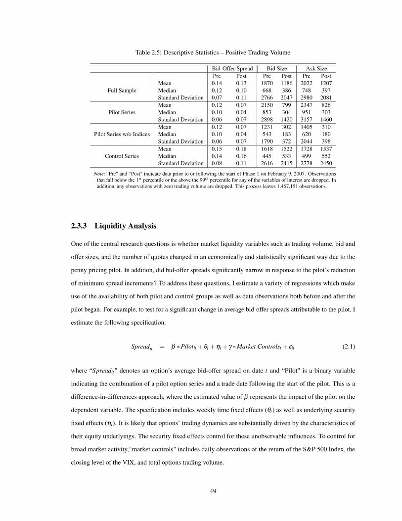
Table 2.5: Descriptive Statistics – Positive Trading Volume

Bid-Offer Spread Bid Size Ask SizePre Post Pre Post Pre Post

Full SampleMean 0.14 0.13 1870 1186 2022 1207Median 0.12 0.10 668 386 748 397Standard Deviation 0.07 0.11 2766 2047 2980 2081

Pilot SeriesMean 0.12 0.07 2150 799 2347 826Median 0.10 0.04 853 304 951 303Standard Deviation 0.06 0.07 2898 1420 3157 1460

Pilot Series w/o IndicesMean 0.12 0.07 1231 302 1405 310Median 0.10 0.04 543 183 620 180Standard Deviation 0.06 0.07 1790 372 2044 398

Control SeriesMean 0.15 0.18 1618 1522 1728 1537Median 0.14 0.16 445 533 499 552Standard Deviation 0.08 0.11 2616 2415 2778 2450

Note: “Pre" and “Post" indicate data prior to or following the start of Phase 1 on February 9, 2007. Observationsthat fall below the 1st percentile or the above the 99th percentile for any of the variables of interest are dropped. Inaddition, any observations with zero trading volume are dropped. This process leaves 1,467,151 observations.

2.3.3 Liquidity Analysis

One of the central research questions is whether market liquidity variables such as trading volume, bid and

offer sizes, and the number of quotes changed in an economically and statistically significant way due to the

penny pricing pilot. In addition, did bid-offer spreads significantly narrow in response to the pilot’s reduction

of minimum spread increments? To address these questions, I estimate a variety of regressions which make

use of the availability of both pilot and control groups as well as data observations both before and after the

pilot began. For example, to test for a significant change in average bid-offer spreads attributable to the pilot, I

estimate the following specification:

Spreadit = β ∗Pilotit +θt +ηi + γ ∗Market Controlst + εit (2.1)

where “Spreadit" denotes an option’s average bid-offer spread on date t and “Pilot" is a binary variable

indicating the combination of a pilot option series and a trade date following the start of the pilot. This is a

difference-in-differences approach, where the estimated value of β represents the impact of the pilot on the

dependent variable. The specification includes weekly time fixed effects (θt) as well as underlying security

fixed effects (ηi). It is likely that options’ trading dynamics are substantially driven by the characteristics of

their equity underlyings. The security fixed effects control for these unobservable influences. To control for

broad market activity,“market controls" includes daily observations of the return of the S&P 500 Index, the

closing level of the VIX, and total options trading volume.

49

I estimate a variety of regressions, each with a different dependent variable, to look for significant changes

in average bid-offer spreads, trading volume, average transaction size, number of quotes, and size of the best

bid and offer quotes. The results are reported in Tables 2.6-2.8. For these specifications, I restrict the data

sample to the 1,467,151 observations with positive trading volume. As mentioned earlier, positive trading

volume may corroborate the reliability of the data for the other trading variables. To confirm that the exclusion

of zero volume observations is not significantly altering the regression results, I also estimate these regressions

including those observations and report the results in the Appendix. Reassuringly, the findings are consistent

across methods.14

For each equity underlying, I calculate the daily average of each variable across all of the corresponding

option series. This generates a single daily observation for each underlying. As a result, the pilot coefficient

estimate can be interpreted as the impact of including an equity series in the pilot on the corresponding options’

average trading dynamics. Due to my exclusion of observations with zero volume, I only averaged across

bid-offer spreads and bid and offer sizes if the option actually traded on that day. After taking daily averages,

there are 7124 observations.

As reported in Table 2.6, average bid-offer spreads fell by $0.064 due to the pilot and this estimate is

strongly statistically significant. The decrease is substantial compared to the pre-pilot mean spread of $0.12

for the pilot option series. Given an average daily trading volume of 269,940 contracts for the pilot option

series, the decrease in bid-offer spreads is equivalent to transaction cost “savings" of $1.7 million each day

(using a contract multiplier of 100). Alternatively, this can be thought of as a loss in profits for market makers.

Average trading volume increased by 10.6 contracts, which is approximately a 10 percent increase relative

to pre-pilot trading volume. However, this estimate is not statistically significant. The number of price

quotes increased by 1542 on average, an economically and statistically significant change. The pilot also

had a substantial impact on the average inside bid and offer sizes, with declines both large in magnitude

and statistically significant. To put these changes in perspective, the best bid and offer sizes declined by

approximately 52% compared to the pre-pilot means.

I also estimate these regressions using observations for each option series rather than calculating daily

averages for each equity underlying. This captures the effect of the pilot on individual options series, but

is harder to interpret as the impact of the SEC adding an underlying equity name to the pilot. The results

are similar to those reported for the averages in Table 2.6. The magnitude of the pilot securities’ increase in

volume rises to 15.2 and the pilot coefficient for the average transaction size regression increases to 4.2 but

both estimates remain statistically insignificant. The declines in bid and offer sizes and the increase in the

14The results are slightly stronger in magnitude for the sample which excludes observations with zero volume. A formal analysis of theimpact of the pilot on the probability of positive trading volume is presented in Section 2.3.4.

50

number of quotes are slightly larger in magnitude and remain strongly statistically significant. Overall, the

estimated impact of the pilot on individual option series is stronger than the estimated impact on the averages

across the options corresponding to each equity underlying.

Table 2.6: Market Impact

Dependent Variable Bid-Offer Trading Bid Offer Number of Avg TransactionSpread Volume Size Size Price Quotes Size

Pilot Coefficient −0.064∗∗∗ 10.6 −1131∗∗∗ −1228∗∗∗ 1542∗∗∗ 1.9S.E. 0.005 6.0 266.6 297.1 499.2 2.6∗ p < 0.10, ∗∗ p < 0.05, ∗∗∗ p < 0.01. Standard errors are clustered by underlying security and date.

Note: “Pilot Coefficient" is the coefficient estimate on a binary variable which takes a value of one for pilot series on tradedates after the start of Phase 1 on February 9, 2007. Full sets of time and underlying security fixed effects are included in allspecifications as well as market controls. Observations with zero trading volume are dropped and averages are calculatedsuch that there is a single daily observation for each equity underlying. This process leaves 7124 observations.

Table 2.7: Market Impact without Averaging

Dependent Variable Bid-Offer Trading Bid Offer Number of Avg TransactionSpread Volume Size Size Price Quotes Size

Pilot Coefficient −0.074∗∗∗ 15.2 −1253∗∗∗ −1337∗∗∗ 1994∗∗∗ 4.2S.E. 0.006 8.5 375.0 427.6 685.3 4.3∗ p < 0.10, ∗∗ p < 0.05, ∗∗∗ p < 0.01. Standard errors are clustered by underlying security and date.

Note: “Pilot Coefficient" is the coefficient estimate on a binary variable which takes a value of one for pilot series on tradedates after the start of Phase 1 on February 9, 2007. Full sets of time and underlying security fixed effects are includedin all specifications as well as market controls. Observations with zero trading volume are dropped, leaving 1,467,151observations. Each observation is daily data for a single option series.

Given these results, it is worthwhile to look in greater detail at the decline in observed bid-offer spreads.

During the six months prior to the start of the pilot, 12.5% of the pilot series and 9.9% of the control series

were quoted at the five-cent minimum increment.15 Following the start of the pilot, 8.7% of the control series

were quoted at the maintained five-cent minimum increment. In contrast, 39.9% of the pilot series were

quoted with bid-offer spreads equal to or less than five cents. Of this percentage, 4.2% of the quotes were

at the new penny minimum increment.16 Histograms of these bid-offer spread distributions are presented

below. These statistics confirm that pre-pilot minimum quote increments were binding constraints for market

makers and suggest a broad narrowing of bid-offer spreads due to the greater price competition. Not only did

bid-offer spreads fall from five-cents to a smaller quantity, but series previously quoted with spreads wider

than five-cents also joined the sub-five-cent group.17

15This suggests higher pre-pilot liquidity of pilot series. However, the pilot was announced in the Fall of 2006 and this announcementmay have generated a narrowing of spreads in anticipation of the start of the pilot in February 2007.

16Note that these statistics are the percentage of options series for which the day’s average bid-offer spread was at the minimum increment.The statistics would likely be much larger if they reflected the fraction of options which were quoted at the minimum increment at any

51

Figure 2.1: Distribution of Bid-Offer Spreads

The analysis thus far evaluates the impact of penny pricing on the full pilot group. However, it is plausible

that the impact will differ for different types of options securities. For instance, equity and index options

may respond differently to the reduction in minimum bid-offer spreads, particularly since index series tend to

be more liquid in terms of trading activity and bid and offer sizes. To investigate whether the impact of the

pilot differed for options with equity versus index underlyings, I estimate the same difference-in-differences

regression specifications using a subset of the pilot series that excludes index options. Of the thirteen Phase 1

pilot series, three have index underlyings: IWM, QQQQ and SMH. The results are reported in Table 2.8.

Table 2.8: Market Impact Excluding Index Options

Dependent Variable Bid-Offer Trading Bid Offer Number of Avg TransactionSpread Volume Size Size Price Quotes Size

Pilot Coefficient −0.061∗∗∗ 4.9 −821∗∗∗ −942∗∗∗ 1031∗∗ -0.46S.E. 0.006 5.2 185.7 228.6 459.2 1.4∗ p < 0.10, ∗∗ p < 0.05, ∗∗∗ p < 0.01. Standard errors are clustered by underlying security and date.

Note: “Pilot Coefficient" is the coefficient estimate on a binary variable which takes a value of one for pilot series ontrade dates after the start of Phase 1 on February 9, 2007. Options series with index underlyings are dropped fromthe data set. Full sets of time and underlying security fixed effects are included in all specifications as well as marketcontrols. Observations with zero trading volume are dropped and averages are calculated such that there is a single dailyobservation for each equity underlying. This process leaves 5480 observations.

point during the trading day.17These statistics are calculated using the data set which retains observations with zero trading volume. The numbers are even more

extreme when these observations are excluded: Prior to the pilot, 3.3% of pilot series and 1.4% of control series were quoted at thefive-cent minimum increment. Following the start of the pilot, 1.4% of the control series continued to be quoted at the five-centminimum. In contrast, 57.5% of pilot series were quoted with bid-offer spreads less than or equal to five cents. However, of thispercentage, only 0.5% were quoted at the penny minimum.

52

The decline in bid-offer spreads is nearly identical to that for the pilot group as a whole. The main difference

between the results is a smaller increase in trading volume compared to that found for the combined group.

In addition, the average transaction size for options corresponding to equity rather than index underlyings

shows a small decline due to the pilot, although this estimate is not statistically significant. While the pilot

reduced bid-offer spreads for all pilot options series, these results indicate that equity options are less likely to

experience the gains in trading volume predicted by the SEC. In addition, the average bid and offer sizes for

equity options responded more strongly relative to their pre-pilot mean values. In particular, the bid and offer

sizes declined approximately 67% compared to the pre-pilot means, versus a 52% decline for the pilot group

as a whole.

While the declines in bid and offer quote sizes are certainly substantial, it is logical that the quote sizes will

fall once there are a greater number of price points across which the quantities can be spread. A reasonable

question is whether these changes are more or less extreme than those expected due to the change in minimum

pricing increments. To make this point clear, suppose there are 100 contracts at the best bid and offer with a

five-cent minimum increment. If this quantity is divided equally among the five price points when we move to

penny increments, we would expect to observe 20 contracts at the best bid and offer. This would be an 80%

decline in the size of the inside quotes.

As discussed above, the data shows a 52% decline in quotes sizes for the full pilot group and a 67% decline

for the pilot series with equity rather than index underlyings. Therefore, the decline is not as extreme as the

scenario where quote quantities are equally spread across all available price points.18 On the other hand, a

relevant issue is whether the post-pilot bid and offer quote sizes are large enough to satisfy the trading needs of

institutional customers who typically trade large quantities and prefer to have immediate trade execution rather

than piecing in orders at different prices. The dramatic decline in quote sizes underlies the concern expressed

by some market participants that the pilot has resulted in insufficient liquidity for institutional traders. This

issue is discussed in detail in Section 2.4.2.

2.3.4 Probit Analysis

As illustrated by the descriptive statistics reported in Section 2.3.2, the majority of option series do not trade

each day. In addition to the various measures evaluated in the previous section, the probability that a security

trades on a given day is a relevant measure of market liquidity. The following analysis investigates whether the

pilot has affected the extrinsic margin of liquidity.

18This may be explained by the fact that bid-offer spreads did not come down to a penny for all pilot securities.

53

To give a preliminary sense of the Phase 1 data, the percentage of daily observations with positive trading

volume increased from 14.8% before the pilot to 19.5% after the pilot for the pilot securities.19 In contrast,

the percentage of positive trading volume observations for the control series increased by a much smaller

margin, from 17.2% to 17.9%. What could explain these relative changes? The reduction in the minimum

quote increment from a nickel to a penny creates more price points at which market makers can potentially

provide quotes. The more detailed menu of price quotes combined with the reduction in transaction costs

via bid-offer spreads may encourage investors to trade not only a greater number, but also a wider variety of

options. This would be consistent with the SEC’s expectations for the pilot to stimulate trading activity.

In order to assess the impact of the pilot on the probability that an option security trades on a given day, I

estimate the following probit specification:

Pr(Volumeit > 0|Xit) = Φ(β0 +β1 ∗Pilot Periodt +β2 ∗Pilot Seriesi

+ β3 ∗ (Pilot Period * Pilot Series)it +

+ γ ∗Market Controlst) (2.2)

where “Pilot Period" and “Pilot Series" are binary variables denoting a trade date following the start of the

pilot and a pilot option series, respectively. The probit results are reported as marginal effects in Tables 2.10

and 2.11, reflecting the impact of a discrete change from 0 to 1 for each binary variable. The results indicate

that the probability of positive trading volume increased by 4.4% for the pilot series following the start of

Phase 1. The results are consistent with the theory that lower transaction costs and a finer grid of price points

have attracted broader investor trading interest.

I estimate the same specification for options with equity rather than index underlyings and find no

significant effect on trading probabilities. This complements the finding in the previous section that the

increase in trading volume experienced by the full pilot group is not nearly as apparent when equity options

are considered separately. In other words, the expectations for the pilot to stimulate trading have not been

convincingly achieved for equity options.

The model presented by Glosten and Milgrom (1985) suggests an additional dimension to the relationship

between the pilot implementation and the probability of positive trading volume. If the risks of asymmetric

information are greater for less frequently traded options, market makers may have less incentive to provide

quotes for far-out-of-the-money or longer dated options following the pilot’s reduction in bid-offer spreads.20

19An observation with zero volume represents an option security that was quoted by market makers during the trading day, but thesequotes did not result in a trade.

20Market makers need not quote at the minimum penny increment. The willingness to trade at different spreads may reflect differences inmarket makers’ information, risk-taking preferences or inventory costs.

54

Instead, a market maker may now only volunteer price quotes on a subset of the original menu of options

securities.

Options which are far “in" or “out" of the money trade less frequently, in lower volume, and at wider

bid-offer spreads, making them relatively illiquid securities. This illiquidity is relative to that of actively

“in-play" options for which the strike price is close to the current stock price.21 For a call option, a positive

value of “moneyness" denotes a current stock price greater than the exercise price and a negative value denotes

a stock price below the exercise price. The opposite relationships hold for put options. To test whether the

change in the number of quotes varied with the “moneyness" of the pilot options, I estimate:

Quotesit = β1Pilotit +β2Moneynessit +β3Pilot * Moneynessit

+ θt +ηi + γ ∗Market Controlst + εit (2.3)

where “Pilot" is a binary variable indicating the combination of a pilot option series and a trade date following

the start of the pilot. Since options which are far in- or out-of-the-money are similarly illiquid, I use the

absolute value of moneyness as the explanatory variable. The results reported in Table 2.9 illustrate that there

are relatively fewer price quotes for options with higher absolute moneyness and this effect is magnified for

the pilot securities following the start of Phase 1.

Table 2.9: Market Maker Quotes

Dependent Variable: Pilot |Moneyness | |Moneyness | * PilotQuotesEstimate 2558∗∗∗ −81.4∗∗∗ −173.7∗∗∗

S.E. 812.4 17.0 33.1∗ p < 0.10, ∗∗ p < 0.05, ∗∗∗ p < 0.01. Standard errors are clustered by underlyingsecurity and date.

Note: “Pilot" is a binary variable which takes a value of one for pilot securities fol-lowing the start of the pilot on February 9, 2007. Underlying and weekly time fixedeffects are included in addition to market control variables.

A reduction in the breadth of market maker price quotes may result in a lower probability that a trade takes

place for options which are far in- or out-of-the-money. I evaluate this possibility by looking at how the probit

results change when the absolute value of moneyness is included as a control in the specification. As reported

in Tables 2.10 and 2.11, the coefficient estimates for the interaction term between moneyness and the pilot

indicator variable are negative and statistically significant. The pilot securities experienced a 16.8% increase

in the probability of positive trading volume, but a small increase in the absolute value of moneyness (i.e. a

21Dividing the options into quartiles according to their pre-pilot absolute value of moneyness (a lower quartile denotes an option with astrike closer to the current stock price), the mean value of pre-pilot daily trading volume for each quartile is as follows: 31.6 for Quartile1, 8.4 for Quartile 2, 4.2 for Quartile 3, and 2.7 for Quartile 4. The mean pre-pilot bid-offer spread for each quartile is as follows: 0.159for Quartile 1, 0.169 for Quartile 2, 0.177 for Quartile 3, and 0.193 for Quartile 4.

55

strike price farther away from the current stock price) decreases this probability by approximately 1.6%.

The observed gains in trading probabilities attributable to the pilot are concentrated among option securities

which are in the more active region where the strike price is close to the current stock price. Options with

strike prices farther from the current stock price are typically less liquid and are therefore potentially riskier

securities for market makers to trade due to information asymmetries or high inventory costs. The relatively

lower probability of a trade following the start of the pilot may reflect an unwillingness of some market makers

to quote prices for these risky securities given the lower potential profits offered by the narrower bid-offer

spreads.

Table 2.10: Probability of Positive Trading Volume

Pilot Pilot Pilot |Moneyness | |Moneyness |Period Series * Pilot

Estimate -0.009 -0.026 0.044∗∗∗

S.E. 0.010 0.068 0.016Estimate -0.002 -0.045 0.168∗∗∗ -0.003 −0.016∗∗∗

S.E. 0.013 0.055 0.065 0.002 0.006∗ p < 0.10, ∗∗ p < 0.05, ∗∗∗ p < 0.01. Standard errors are clustered by underlyingsecurity.

Note: The reported estimates are marginal effects reflecting the impact of a discretechange from 0 to 1 for each binary variable. “Pilot" is a binary variable which takesa value of one for pilot securities following the start of the pilot on February 9, 2007.Observations with zero trading volume are retained, leaving 9,660,993 observations.Market controls are included in all specifications.

Table 2.11: Probability of Positive Trading Volume Excluding IndexOptions

Pilot Pilot Pilot |Moneyness | |Moneyness |Period Series * Pilot

Estimate 0.019∗ 0.019 0.010S.E. 0.010 0.044 0.012Estimate 0.024∗∗ 0.008 0.130∗∗∗ -0.003 −0.016∗∗

S.E. 0.011 0.044 0.051 0.003 0.007∗ p < 0.10, ∗∗ p < 0.05, ∗∗∗ p < 0.01. Standard errors are clustered by underlyingsecurity.

Note: The reported estimates are marginal effects reflecting the impact of a discretechange from 0 to 1 for each binary variable. “Pilot" is a binary variable which takesa value of one for pilot securities following the start of the pilot on February 7, 2007.Observations with zero trading volume are retained, leaving 4,076,874 observations.Market controls are included in all specifications.

56

2.3.5 Transition Dynamics

Despite the discrete start of the Penny Pilot on February 9, 2007, the adjustment of bid-offer spreads may have

been a gradual process. Rather than immediately reducing the bid-offer spreads for the pilot series, it may

have taken time for market makers to adjust to the new pricing system. One way to test for a transition process

is to estimate a regression with a quadratic time trend beginning at the start of Phase 1. Using both the control

and pilot series, I estimate the following specification:

Spreadit = β0 +β1 ∗Weekst +β2 ∗Weeks2t +β3 ∗Pilot Seriesi

+ β4 ∗ (Weeks∗Pilot Series)it +β5 ∗ (Weeks2 ∗Pilot Series)it + εit (2.4)

where “Weeks" is the number of weeks since the start of the pilot on February 9, 2007, and “Pilot Series" is a

binary variable indicating that the underlying is included in the pilot. Compared to a simple linear trend, the

quadratic specification allows me to capture an evolving market transition. All specifications include the daily

S&P 500 Index return, closing level of the VIX, and total options trading volume as market controls.

I also estimate this transition regression with trading volume, average bid and offer sizes, and the number

of market maker quotes as dependent variables. Similar to the story for bid-offer spreads, market makers

may have drastically cut inside bid and offer sizes at the beginning of the pilot and then gradually increased

liquidity as time passed and they became more accustomed to the new pricing system. A change in trading

volume over time would provide information about the gradual impact of the pilot on investor trading interest.

The estimates are reported in Table 2.12.

The coefficient estimate in the bid-offer spread regression is negative for both the linear and squared

interaction terms. Neither of these estimates is statistically significant, suggesting an immediate and stable

market response of spreads to the pilot implementation. The number of market maker price quotes has

increased over time while trading volume and bid and offer quote sizes have decreased over time. All of these

variables are changing at decreasing rates. Other than the statistically significant coefficients for the evolution

of the average bid size, the coefficients in these regressions are not statistically significant. In other words,

the results indicate that the dramatic changes observed for these variables primarily occurred immediately

following the start of the pilot and have persisted over time.

Another strategy for analyzing the transition dynamics following the start of the pilot is to use a

Kolmogorov-Smirnov (K-S) test of the homogeneity of the distribution of bid-offer spreads. In particu-

lar, I use the K-S distance statistic to evaluate whether the distribution of spreads was significantly different

between the pre-pilot period and various post-pilot periods, where the post-pilot periods differ according to

57

Table 2.12: Transition Dynamics

Weeks Weeks2 Pilot Weeks * Weeks2 *Dependent Variable Series Pilot Series Pilot Series

Average Bid-Offer SpreadEstimate -0.0007 0.0001∗∗∗ −0.083∗∗∗ -0.0001 -0.00004S.E. 0.0006 0.00002 0.016 0.001 0.00003

Average Bid SizeEstimate -0.30 0.0005 -36.2 −10.0∗∗∗ 0.33∗∗∗

S.E. 2.44 0.10 207.4 2.5 0.11

Average Offer SizeEstimate −10.3∗∗∗ 0.26 -97.8 -5.7 0.23S.E. 4.5 0.18 277.8 4.6 0.22

Trading VolumeEstimate 0.03 -0.001 9.2 -0.23 0.005S.E. 0.21 0.006 5.8 0.25 0.007

QuotesEstimate 12.2 -0.14 -37.6 46.2 -1.8S.E. 30.7 0.91 546.8 37.8 1.3

∗ p < 0.10, ∗∗ p < 0.05, ∗∗∗ p < 0.01. Standard errors are clustered by underlying security.Note: “Weeks" is the number of weeks since the start of Phase 1 on February 9, 2007. This is interacted with a binary variable

taking a value of one for pilot options to generate “Weeks * Pilot Series". Market controls are included in all specifications.Observations with zero trading volume are retained and averages are calculated such that there is a single daily observationfor each equity underlying. This leaves 3666 observations following the start of the pilot.

the omitted adjustment period. The advantage of the K-S test is its ability to look at the full distribution of

bid-offer spreads rather than the first-moment alone, as in the difference-in-differences estimation of Section

2.3.3. In addition, it allows me to look at the evolution of the distribution across the post-pilot period. I

estimate the following specification separately for the pre- and post-pilot periods using daily trading data for

each option series:

Spreadit = β ∗Pilot Seriesi +θt +ηi + γ ∗Market Controlst + εit (2.5)

Underlying security fixed effects are denoted by ηi and weekly time fixed effects by θt . I re-fit the model for

the post-pilot dates omitting the first week (February 9, 2007 - February 16, 2007), then omitting the first

and second weeks, then omitting the first, second and third weeks, and so on. I perform K-S tests comparing

the distribution of the regression residuals between the pre-pilot period and the various post-pilot periods,

giving me a sequence of K-S statistics for different partitions of the data set. The variation in the number of

omitted post-pilot weeks allows for different adjustment periods between the pre- and post-pilot equilibria of

the distribution of bid-offer spreads. Essentially, this process identifies the post-pilot equilibrium of bid-offer

spreads as the difference between the K-S statistics for different post-pilot periods gradually declines.

The K-S distance statistics for the different data partitions are displayed in Figure 2.2. The p-values for

all of the data partitions are zero, resulting in rejection of the null hypothesis that the distributions of pre-

and post-pilot spreads are equal. The difference between the pre- and post-pilot bid-offer spread distributions

continues to increase until week 24 (August 7, 2007) at which point the difference falls off. The sharp change

at the end of the sample period is likely an artifact of the small number of observations once I allow the

58

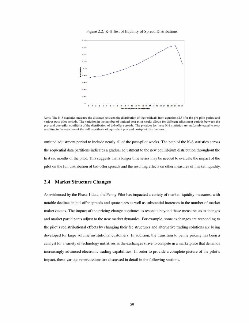
Figure 2.2: K-S Test of Equality of Spread Distributions

Note: The K-S statistics measure the distance between the distribution of the residuals from equation (2.5) for the pre-pilot period andvarious post-pilot periods. The variation in the number of omitted post-pilot weeks allows for different adjustment periods between thepre- and post-pilot equilibria of the distribution of bid-offer spreads. The p-values for these K-S statistics are uniformly equal to zero,resulting in the rejection of the null hypothesis of equivalent pre- and post-pilot distributions.

omitted adjustment period to include nearly all of the post-pilot weeks. The path of the K-S statistics across

the sequential data partitions indicates a gradual adjustment to the new equilibrium distribution throughout the

first six months of the pilot. This suggests that a longer time series may be needed to evaluate the impact of the

pilot on the full distribution of bid-offer spreads and the resulting effects on other measures of market liquidity.

2.4 Market Structure Changes

As evidenced by the Phase 1 data, the Penny Pilot has impacted a variety of market liquidity measures, with

notable declines in bid-offer spreads and quote sizes as well as substantial increases in the number of market

maker quotes. The impact of the pricing change continues to resonate beyond these measures as exchanges

and market participants adjust to the new market dynamics. For example, some exchanges are responding to

the pilot’s redistributional effects by changing their fee structures and alternative trading solutions are being

developed for large volume institutional customers. In addition, the transition to penny pricing has been a

catalyst for a variety of technology initiatives as the exchanges strive to compete in a marketplace that demands

increasingly advanced electronic trading capabilities. In order to provide a complete picture of the pilot’s

impact, these various repercussions are discussed in detail in the following sections.

59

2.4.1 Maker Taker

Returning to a point made earlier in the paper, the penny pilot has effectively redistributed the gains of

innovation from the exchanges’ market makers to investors. The narrower bid-offer spreads create a potential

tradeoff between a reduction in market frictions for investors, via reduced transaction costs and greater price

transparency, and market makers’ incentives to provide liquidity. Considering their exposure to inventory costs

and information asymmetries, wider bid-offer spreads may by necessary to encourage market makers to quote

and trade options. As illustrated in the previous section, trading volume has not increased enough for the pilot

to benefit market makers despite the narrower spreads. This is particularly true for options with equity rather

than index underlyings.

In support of the incentive theory, some exchanges have begun redesigning their fee structures to reward

market markers for providing liquidity and charge investors for extracting liquidity. This new fee schedule is

called “maker-taker." Following the execution of a trade, the market maker or institution who provided the

original quote receives a payment while the investor pays a fee on top of the standard brokerage charges. In

addition to providing direct incentives for market participants to provide liquidity, maker-taker influences the

prices at which market makers are willing to trade. In particular, market makers are willing to trade not only at

less profitable prices, but perhaps even unprofitable prices as long as the loss is offset by the liquidity payment.

Interestingly, only some of the options exchanges have adopted the maker-taker fee model. In addition, the

fees charged differ across exchanges. This variation among the exchanges’ fee structures raises an important

question: If some exchanges do not charge anything while others charge taker fees which potentially differ

across exchanges, is the transparency of a security’s true price at risk? The SEC has responded to this concern

by noting that exchanges have traditionally maintained different transaction fee models and that there is not

cause for concern provided the taker fees remain less than the minimum bid-offer spread increment of a penny

(equivalent to $1 per contract as there are 100 options per contract). However, without further regulation the

fees seem to jeopardize a potentially significant portion of the investor gains from penny pricing.

2.4.2 Institutional Investors and Alternative Trading Venues

Several market participants are concerned that thinner markets due to penny pricing will drive larger insti-

tutional investors away from public exchanges to either the well-established over-the-counter broker-dealer

markets or to “dark pool" trading networks similar to those available in the equity market.22 To put the

difference in perspective, retail investors trade an average of 15 options contracts per trade while institutional

investors trade 1,000 contracts or more. A decline in available trading size at each price point therefore has a

22Recent financial market crises have generated concern about counterparty risk. This may encourage movement away from the OTCmarket and back to the exchanges, where counterparty obligations are guaranteed by the Options Clearing Corporation.

60

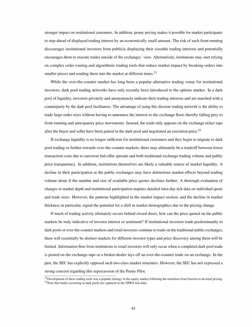
stronger impact on institutional customers. In addition, penny pricing makes it possible for market participants

to step ahead of displayed trading interest by an economically small amount. The risk of such front-running

discourages institutional investors from publicly displaying their sizeable trading interests and potentially

encourages them to execute trades outside of the exchanges’ view. Alternatively, institutions may start relying

on complex order routing and algorithmic trading tools that reduce market impact by breaking orders into

smaller pieces and sending them into the market at different times.23

While the over-the-counter market has long been a popular alternative trading venue for institutional

investors, dark pool trading networks have only recently been introduced to the options market. In a dark

pool of liquidity, investors privately and anonymously indicate their trading interests and are matched with a

counterparty by the dark pool facilitators. The advantage of using this discrete trading network is the ability to

trade large order sizes without having to announce the interest to the exchange floor, thereby falling prey to

front-running and anticipatory price movements. Instead, the trade only appears on the exchange ticker tape

after the buyer and seller have been paired in the dark pool and negotiated an execution price.24

If exchange liquidity is no longer sufficient for institutional customers and they begin to migrate to dark

pool trading or further towards over-the-counter markets, there may ultimately be a tradeoff between lower

transaction costs due to narrower bid-offer spreads and both traditional exchange trading volume and public

price transparency. In addition, institutions themselves are likely a valuable source of market liquidity. A

decline in their participation at the public exchanges may have deleterious market effects beyond trading

volume alone if the number and size of available price quotes declines further. A thorough evaluation of

changes in market depth and institutional participation requires detailed intra-day tick data on individual quote

and trade sizes. However, the patterns highlighted in the market impact section, and the decline in market

thickness in particular, signal the potential for a shift in market demographics due to the pricing change.

If much of trading activity ultimately occurs behind closed doors, how can the price quoted on the public

markets be truly indicative of investor interest or sentiment? If institutional investors trade predominantly in

dark pools or over-the-counter markets and retail investors continue to trade on the traditional public exchanges,

there will essentially be distinct markets for different investor types and price discovery among them will be

limited. Information flow from institutions to retail investors will only occur when a completed dark pool trade

is posted on the exchange tape or a broker-dealer lays off an over-the-counter trade on an exchange. In the

past, the SEC has explicitly opposed such two-class market structures. However, the SEC has not expressed a

strong concern regarding this repercussion of the Penny Pilot.

23Development of these trading tools was a popular strategy in the equity market following the transition from fraction to decimal pricing.24Note that trades occurring in dark pools are captured in the OPRA tick data.

61

2.4.3 Incentives for Further Technological Progress

A broad issue highlighted by this study of the Penny Pilot is the SEC’s role in either promoting or constraining

the further development of technology and the diffusion of innovation. In mandating the pilot, the SEC has

required the capabilities of existing technology be put to full use. However, if the gains from these technology

improvements are redistributed to investors via narrower pricing spreads, how will the exchanges’ incentives

to invest in further innovation be affected?

While trading volume has not increased in response to the pilot, penny pricing has forced exchanges to

aggressively compete for existing market share by focusing on the quality of their technological capabilities.

Through its reliance on advanced electronic trading infrastructure, penny pricing gives technology differences

a greater role in differentiating the exchanges. In particular, penny pricing increases the importance of quote

and execution speed, data capacity, and electronic connectivity among market participants.

In addition, the exchanges are developing trading tools to help institutional investors manage larger trades,

similar to the algorithms and complex routing strategies used in the equity market. Penny pricing may also

lead to electronic market surveillance and order routing, known as “smart-routing" technology, as it becomes

difficult to manually process and respond to the increased granularity of quotes displayed in penny increments.

One of the greatest incentives for technology development is the sheer volume of quote data generated by

penny pricing, which allows for five times as many price points per dollar and requires more frequent price

updates. In order to keep the electronic trading systems running smoothly, quote mitigation technology is an

essential priority for the exchanges in order to reduce the quantity of data flowing through the inter-exchange

communication networks.25

2.5 Conclusion

The Penny Pilot highlights the complex interaction of technology, regulation, and market development in

the equity options market. Despite the reservations of some exchanges and concerns regarding various

repercussions of the pilot, the SEC maintains a positive stance regarding the impact of penny pricing and

recently announced an expansion of the pilot that will ultimately encompass over 85 percent of all options

trading volume.26 As evident from the changes already adopted, the market continues to evolve in response to

the challenges presented by penny pricing. These challenges include thinner markets, growing data capacity

and speed requirements, and competition from alternative trading venues. The technology demands intrinsic25One strategy which has been implemented by CBOE and ISE is a holdback timer that aggregates all of the quote changes submitted by

market makers and only submits the best bid-offer quotes to OPRA. In order to prevent any noticeable pricing delays, this entire processoccurs in less than one second.

26On September 23, 2009, the SEC announced that 300 additional options will be transitioned to penny pricing within the following year.This brings the total number of equity option series trading in penny increments to 363. The 63 options series included in the first threephases of the pilot represent approximately 50 percent of total options trading volume.

62

to penny pricing combined with the risk of losing institutional customer business have provided substantial

incentives for the exchanges to continue innovating.

As the impact of penny pricing continues to develop, there are a number of ways to extend the work

presented in this paper. The first is to dig deeper into the various reactions of the exchanges. As mentioned

earlier, sophisticated technology is a competitive advantage with penny pricing. Smaller exchanges such as

NYSE Arca, BOX and Nasdaq may support penny pricing because it provides an opportunity to compete with

the traditional, large market share exchanges by showcasing their technological capabilities. In order to fully

understand the exchanges’ evolving positions, a separate analysis of the market impact of penny pricing for

each exchange is necessary. OPRA’s intra-day tick data designates the exchange providing each quote or trade

execution. Using this data, it is possible to compare trading patterns across the exchanges. While that would

be a valuable next step, the data used in this paper provides an overview of the changing market dynamics and

identifies patterns to investigate more closely using exchange-specific data.

Another promising extension would incorporate data for Phases 2 and 3 of the pilot and evaluate the longer

term impact of the pricing change. An interesting aspect of the Phase 2 data is the inclusion of options on both

the S&P 500 Index (SPX) and the S&P 500 SPDR (SPY). The only difference between the two is that the SPY

trades at one-tenth the price of the SPX. As a result, retail investors tend to trade SPY and its corresponding

options while institutions trade SPX and its corresponding options. The same is true for the Dow Jones

Industrial Average (DJX) and the Diamonds Trust (DIA), both of which were included in Phase 2. Analyzing

the response of these securities to the pricing change would provide insight into the differences between the

trading behavior of retail versus institutional investors and the potential divergence in their experiences with

the pilot.27

Beyond an analysis of the impact of penny pricing, this case study provides a valuable example of

the complex relationship between a market and its regulators. As is often the case, the implementation

of a regulatory change can generate a complicated market response that includes a variety of unexpected

repercussions. The details of this case study highlight the SEC’s substantial power in shaping the equity

options market’s innovations and competitive environment. Following the ongoing market developments and

considering them in light of the SEC’s continuing regulatory involvement will be important in fully assessing

the emerging implications of the technological innovations that set this process in motion.

27In addition, options on SPX and DJX only trade at CBOE, permitting an exchange-specific analysis of the pilot’s liquidity impact.

63

2.6 Appendix

2.6.1 Control Selection

The panel of securities includes the thirteen Phase 1 series as well as a selection of comparable securities to

use as controls. These securities are listed in Tables 2.13 and 2.14. Due to data limitations, I was unable to use

the full universe of non-pilot options series as controls. Instead, I needed to select a short list of comparables

before gaining access to the corresponding OPRA data.

Given this limitation, I selected comparables according to five dimensions: (1) industry membership for the

equity series and index nature for the index series; (2) equity market capitalization; (3) equity trading volume

(4) options trading volume; and (5) options open interest.28 The goal of this approach is to select comparables

with trading and liquidity properties similar to those of the pilot series before the implementation of the pilot.

Accordingly, I made comparisons using data for the period from January 1, 2006 through December 31, 2006

which falls safely before the introduction of the pilot in February 2007. Equity market capitalization and

equity trading volume are both highly correlated with the corresponding options’ liquidity and are therefore

logical dimensions to consider in the selection process. Drawing comparables from the same industries as

the pilot series allows me to control for industry characteristics and events which affect liquidity. For index

options, I chose comparables based on whether the index is a broad market index or a sector-specific index.29

The relevant criteria statistics are reported in Tables 2.13 and 2.14.

A more mechanical selection process would begin with the full universe of equity names (those with

options) and use an algorithm to select controls. For each pilot security, the algorithm would consider equity

names which are members of the same industry and then assign weights to various measures such as market

capitalization, average daily equity and options trading volume, and open interest. The equity underlyings

which maximize the selection objective function would be the optimal controls. The benefit of this method is

its ability to look across a broad range of potential securities and objectively select appropriate controls. In

this paper, I use controls which I manually selected. However, such an algorithm approach would be valuable

to confirm the validity of my selections.

Data on the pre-pilot trading dynamics of the Phase 1 securities is also useful to evaluate whether the

group is truly a representative sample, as claimed by the SEC. Note that the majority of the Phase 1 pilot

series come from the computer hardware, semiconductor, and related industries. In addition, they tend to be

the large, dominant players within these industries. This raises doubt that Phase 1 included a representative

28Open interest is the number of outstanding exchange-traded options contracts and is therefore an alternative measure of trading activity.29Since SMH is a narrow index of semiconductor companies, the best comparable is OIH, a narrow index of oil services companies which

has similar trading properties to SMH. In addition, many of the other pilot and control series are members of the SMH index: ADI,AMD, AMKR, JBL, INTC, NVDA, TXN.

64

sample of securities. In particular, it is difficult to know whether the market impact of the pilot would be the

same for options on smaller firms within the semiconductor and computer hardware industries or for options

on firms in other industries with potentially different trading dynamics. Phases 2 and 3 of the pilot include

options series from the financial, energy, automotive and retail industries. An analysis of these pilot phases

will provide valuable information regarding the impact of the regulatory change on the options of a much

broader collection of companies.

65

Tabl

e2.

13:P

hase

1Se

curi

ties

Phas

e1

Equ

ity/I

ndex

Indu

stry

Mar

ketC

apA

vera

geD

aily

Ave

rage

Dai

lyO

pen

Secu

ritie

sE

quity

Trad

ing

Opt

ions

Trad

ing

Inte

rest

Volu

me

Volu

me

1.A

gile

ntTe

ch(A

)E

quity

Ele

ctro

nic

Inst

rum

ents

and

Con

trol

s5.

7B4.

5M37

7811

3,76

62.

Adv

ance

dM

icro

Dev

ices

(AM

D)

Equ

itySe

mic

ondu

ctor

s1.

4B17

.5M

51,3

6595

6,97

33.

Cat

erpi

llar(

CA

T)

Equ

ityC

onst

ruct

ion

and

Agr

icul

tura

lMac

hine

ry25

.8B

13M

28,7

9738

6,57

54.

Flex

tron

ics

Inte

rnat

iona

l(FL

EX

)E

quity

Sem

icon

duct

ors

2.0B

13.7

M27

6115

6,57

95.

Gen

eral

Ele

ctri

c(G

E)

Equ

ityC

ongl

omer

ates

173.

2B12

8.5M

51,0

431,

512,

062

6.In

tel(

INT

C)

Equ

itySe

mic

ondu

ctor

s80

.3B

79.9

M99

,715

2,72

8,71

67.

Isha

res

Rus

sell

2000

(IW

M)

Inde

xM

isce

llane

ous

8.8B

91.1

M33

0,82

05,

621,

429

8.M

icro

soft

(MSF

T)

Equ

itySo

ftw

are

and

Prog

ram

min

g17

0.1B

90.8

M10

2,70

74,

620,

725

9.N

asda

qPo

wer

shar

es(Q

QQ

Q)

Inde

xM

isce

llane

ous

11.4

B19

4.2M

448,

664

7,07

4,46

010

.Sem

iCon

duct

orH

olde

rs(S

MH

)In

dex

Sem

icon

duct

ors

704.

5M12

.5M

48,7

3795

4,05

111

.Sun

Mic

ro(S

UN

W)

Equ

ityC

ompu

terH

ardw

are

3.1B

10.7

M18

,955

881,

252

12.T

exas

Inst

rum

ents

(TX

N)

Equ

itySe

mic

ondu

ctor

s19

.6B

17.5

M25

,665

560,

538

13.W

hole

Food

s(W

FMI)

Equ

ityR

etai

l(G

roce

ry)

1.4B

3.8M

14,7

4912

4,36

2

Not

e:D

ata

oneq

uity

mar

ketc

apita

lizat

ion

and

aver

age

daily

trad

ing

volu

me

com

esfr

omth

eC

RSP

data

base

.Dat

aon

aver

age

daily

optio

nstr

adin

gvo

lum

ean

dop

enin

tere

stco

mes

from

Opt

ionM

etri

cs.T

hest

atis

tics

are

fort

hepe

riod

from

Janu

ary

1,20

06th

roug

hD

ecem

ber3

1,20

06.

66

Tabl

e2.

14:C

ompa

rabl

eSe

curi

ties

Com

para

ble

Equ

ity/I

ndex

Indu

stry

Mar

ketC

apA

vera

geD

aily

Ave

rage

Dai

lyO

pen

Secu

ritie

sE

quity

Trad

ing

Opt

ions

Trad

ing

Inte

rest

Volu

me

Volu

me

1.Ja

bilC

ircu

it(J

BL

)E

quity

Ele

ctro

nic

Inst

rum

ents

and

Con

trol

s1.

3B3.

2M26

6054

,631

2.N

VID

IAC

orpo

ratio

n(N

VD

A)

Equ

itySe

mic

ondu

ctor

s4.

6B15

.5M

21,5

4135

4,45

63.

Dee

re&

Com

pany

(DE

)E

quity

Con

stru

ctio

nan

dA

gric

ultu

ralM

achi

nery

16.8

B6.

4M71

2611

6,02

24.

Am

korT

echn

olog

y(A

MK

R)

Equ

itySe

mic

ondu

ctor

s37

3.4M

2.6M

3287

95,7

635.

Uni

ted

Tech

nolo

gies

(UT

X)

Equ

ityC

ongl

omer

ates

48.8

B9.

0M65

7816

7,98

86.

Mic

ron

Tech

nolo

gy(M

U)

Equ

ityC

ompu

terS

tora

geD

evic

es2.

3B22

.8M

15,3

3857

3,54

77.

Dia

mon

dsTr

ust(

DIA

)In

dex

Mis

cella

neou

s6.

2B39

.0M

64,2

991,

250,

977

8.A

pple

(AA

PL)

Equ

ityC

ompu

terH

ardw

are

80.0

B41

.7M

146,

363

1,97

0,67

79.

SPD

RTr

ust(

SPY

)In

dex

Mis

cella

neou

s74

.7B

445.

4M25

8,27

03,

803,

372

10.O

ilSe

rvic

eH

olde

rs(O

IH)

Inde

xO

ilSe

rvic

es1.

3B10

.5M

58,4

1052

8,71

711

.Hew

lett-

Pack

ard

(HPQ

)E

quity

Com

pute

rHar

dwar

e86

.7B

24.1

M31

,116

911,

268

12.A

nalo

gD

evic

es(A

DI)

Equ

itySe

mic

ondu

ctor

s5.

5B6.

4M22

6694

,039

13.S

afew

ay(S

WY

)E

quity

Ret

ail(

Gro

cery

)10

.0B

5.2M

1566

47,3

21

Not

e:D

ata

oneq

uity

mar

ketc

apita

lizat

ion

and

aver

age

daily

trad

ing

volu

me

com

esfr

omth

eC

RSP

data

base

.D

ata

onav

erag

eda

ilyop

tions

trad

ing

volu

me

and

open

inte

rest

com

esfr

omO

ptio

nMet

rics

.The

stat

istic

sar

efo

rthe

peri

odfr

omJa

nuar

y1,

2006

thro

ugh

Dec

embe

r31,

2006

.

67

2.6.2 Robustness to Inclusion of Observations with Zero Trading Volume

This section reports difference-in-differences regression results when observations with zero trading volume

are included in the regression analysis rather than dropped. The change in bid-offer spreads for pilot securities

is nearly identical. However, the changes in trading volume, average bid and offer sizes and the number of

price quotes are muted. Recall the regression specification:

Spreadit = β ∗Pilotit +θt +ηi + γ ∗Market Controlst + εit (2.6)

where “Spreadit" denotes an option’s average bid-offer spread on date t and “Pilot" is a binary variable

indicating the combination of a pilot option series and a trade date following the start of the pilot. Underlying

fixed effects are denoted by ηi and weekly time fixed effects are denoted by θt .

Table 2.15: Market Impact Including Zero Volume Observations

Dependent Variable Bid-Offer Trading Bid Offer Number of Avg TransactionSpread Volume Size Size Price Quotes Size

Pilot Coefficient −0.063∗∗∗ 5.1∗∗ −464∗∗∗ −791∗∗∗ 920∗∗ 2.4S.E. 0.006 1.9 146.8 215.4 405.9 10.6∗ p < 0.10, ∗∗ p < 0.05, ∗∗∗ p < 0.01. Standard errors are clustered by underlying security and date.

Note: “Pilot Coefficient" is the coefficient estimate on the binary variable which takes a value of one for pilot series on tradedates after the start of Phase 1 on February 9, 2007. Full sets of time and underlying security fixed effects are includedin all specifications as well as market controls. Observations with zero trading volume are retained and averages arecalculated such that there is a single daily observation for each equity underlying. This process leaves 7124 observations.

Table 2.16: Market Impact Including Zero Volume Observations - Exclude Index Options

Dependent Variable Bid-Offer Trading Bid Offer Number of Avg TransactionSpread Volume Size Size Price Quotes Size

Pilot Coefficient −0.057∗∗∗ 3.3 −325∗∗∗ −683∗∗∗ 516 -6.1S.E. 0.006 2.0 74.7 192.9 345.6 5.8∗ p < 0.10, ∗∗ p < 0.05, ∗∗∗ p < 0.01. Standard errors are clustered by underlying security and date.

Note: “Pilot Coefficient" is the coefficient estimate on a binary variable which takes a value of one for pilot series ontrade dates after the start of Phase 1 on February 9, 2007. Options series with index underlyings are dropped fromthe data set. Full sets of time and underlying security fixed effects are included in all specifications as well as marketcontrols. Observations with zero trading volume are retained and averages are calculated such that there is a single dailyobservation for each equity underlying. This process leaves 5480 observations.

68

Bibliography

Amihud, Y. and H. Mendelson. Asset pricing and the bid-ask spread. Journal of Financial Economics, 17,223–249, 1986.

Bacidore, J. M. The impact of decimalization on market quality: An empirical investigation of the TorontoStock Exchange. Journal of Financial Intermediation, 6, 92–120, 1997.

Bacidore, J. M., R. H. Battalio, and R. H. Jennings. Order submission strategies, liquidity supply, and tradingin pennies on the New York Stock Exchange. Journal of Financial Markets, 6, 337–362, 2003.

Barclay, M. J., T. Hendershott, and D. T. McCormick. Competition among trading venues: Information andtrading on electronic communications networks. Journal of Finance, 58, 2637–2665, 2003.

Bessembinder, H. Trade execution costs and market quality after decimalization. Journal of Financial andQuantitative Analysis, 28, 747–777, 2003.

CBOE. Penny Pilot Program and Quote Mitigation: Regulatory Circular RG06-124. Available athttp://www.cboe.org/legal, 2007a.

CBOE. Penny Pilot Report: June. Available at http://www.cboe.org/hybrid/pennypilot.aspx, 2007b.

CBOE. Penny Pilot Report: May 1, 2007 through September 27, 2007. Available athttp://www.cboe.org/hybrid/pennypilot.aspx, 2007c.

CBOE. Penny Pilot Report: September 28, 2007 through January 31, 2008. Available athttp://www.cboe.org/hybrid/pennypilot.aspx, 2007d.

Chakravarty, S. and A. Dubinsky. Individual investors’ reactions to decimalization: Innovation diffusion infinancial markets. Journal of Economic Psychology, 26, 89–103, 2005.

Chakravarty, S., V. Panchapagesan, and R. A. Wood. Did decimalization hurt institutional investors? Journalof Financial Markets, 8, 400–420, 2005.

Chakravarty, S., R. A. Wood, and R. A. V. Ness. Decimals and liquidity: A study of the NYSE. Journal ofFinancial Research, 75–94, 2004.

Chung, K. H., C. Charoenwong, and D. K. Ding. Penny pricing and the components of spread and depthchanges. Journal of Banking & Finance, 28, 2981–3007, 2004.

Gibson, S., R. Singh, and V. Yerramilli. The effect of decimalization on the components of the bid-ask spread.Journal of Financial Intermediation, 12, 121–148, 2003.

Gloster, L. and P. Milgrom. Bid, ask, and transaction prices in a specialist market with heterogeneouslyinformed trades. Journal of Financial Economics, 14, 71–100, 1985.

Goldstein, M. A. and K. A. Kavajecz. Eighths, sixteenths, and market depth: Changes in tick size and liquidityprovision on the NYSE. Journal of Financial Economics, 125–149, 2000.

ISE. Penny Pilot Analysis. Available at: http://www.ise.com, 2007a.

ISE. Penny Pilot Analysis Phase 2. Available at: http://www.ise.com, 2007b.

69

Kadan, O. So who gains from a small tick size? Journal of Financial Intermediation, 15, 32–66, 2006.

King, E. K. Speech by SEC Staff: Remarks before the 2006 Options Industry Conference. Available at:http://www.sec.gov/news/speech/2006/spch050506ekk.htm, 2006.

Kyle, A. S. Continuous auctions and insider trading. Econometrica, 53, 1315–1335, 1985.

Nazareth, A. L. Speech by SEC Commissioner: Remarks before the Securities Industry Association OptionsMarket Structure Conference. Available at: http://www.sec.gov/news/speech/2006/spch102406aln.htm,2006.

NYSEArca. Understanding economic and capacity impacts of the Penny Pilot. Available athttp://www.nyse.com/productservices/nysearcaoptions.html, 2007.

SEC. The Investor’s Advocate: How the SEC protects investors, maintains market integrity, and facilitatescapital formation. Available at: http://www.sec.gov/about/whatwedo.shtml, 2007a.

SEC. Press Release: SEC Chairman Cox urges options exchanges to start limited penny quoting. 2007b.

Sirri, E. R. Speech by SEC Staff: Keynote speech at the SIFMA 2008 Dark Pools Symposium. Available at:http://www.sec.gov/news/speech/2008/spch020108ers.htm, 2008a.

Sirri, E. R. Speech by SEC Staff: Remarks before the 2008 Options Industry Conference. Available at:http://www.sec.gov/news/speech/2008/spch050208ers.htm, 2008b.

Stoll, H. R. Friction. Journal of Finance, 55, 1479–1514, 2000.

70

Chapter 3

Fails to Deliver: The Price Impact of Naked Short Sales

3.1 Introduction

The effect of short selling on asset prices and trading dynamics is a prominent topic of debate among market

participants, regulators, and the popular press. Company executives often blame manipulative short sellers for

falling share prices and short sellers’ pessimistic views have been deemed “anti-American" in the press. This

paper looks specifically at naked short sales in which the agent effecting the short sale does not borrow a share

to deliver to the buyer. I evaluate the validity of the claim that naked shorting leads to negative excess returns

by creating additional selling pressure.1

Recent regulatory actions by the SEC reflect escalating concern regarding the prevalence of naked short

selling.2 In September 2004, the SEC enacted Regulation SHO which required market compliance with stricter

stock location and delivery protocol beginning in January 2005. The goal of this regulation was to reduce

the occurrence and persistence of “failures to deliver", whereby shares are not delivered to the buyer by the

standard T+3 settlement date (three days following the trade date).3 During the financial crisis of 2008, short

selling was blamed for dramatic declines in the prices of financial stocks and naked short selling was vilified

as being especially manipulative. In response, the SEC temporarily prohibited short sales of financial firms

and tightened rules regarding the delivery of borrowed shares in an attempt to eliminate naked short selling

and resulting failures to deliver.4

1“Naked short selling can allow for the instantaneous creation of excess supply, enabling the potential short-term manipulation of shareprices."[Rick Smith, CEO of TASER International, Oct. 6, 2005]. “Naked short selling has caused damages estimated at close to $100billion and when the strategy is implemented, it can destroy companies and completely wipe out shareholder value." [Christian, Shapiro,and Whalen, Houston Law Review, Nov. 2006].

2“We are particularly concerned about the potential negative effect that substantial and persistent fails to deliver may be having on themarket in some securities. Specifically, these fails to deliver can deprive shareholders of the benefits of ownership - voting, lending, anddividends from issuers. Moreover, they can be indicative of abusive naked short selling, which could be used as a tool to drive down acompany’s stock price. They may also undermine the confidence of investors who may believe that the fails to deliver are evidence ofmanipulative naked short selling in the stock. In turn, issuers may be harmed, as investors may be reluctant to commit capital to a stockthat they believe is subject to abusive naked short selling." [Christopher Cox, Chairman of SEC, July 12, 2006].

3Additional information on Regulation SHO is provided in the Appendix.4The SEC enacted an Emergency Order from July 21 through August 12, 2008 which prohibited naked short sales of 19 financial firms. Inorder to effect a short sale, the shares needed to be pre-borrowed. The SEC’s justification for the Emergency Order was that “[F]alserumors can lead to a loss of confidence [and] panic selling, which may be further exacerbated by ‘naked’ short selling", and as a result,

71

The regulatory focus on short selling has revived debate regarding its effect on asset prices. While many

market participants have demanded stronger restrictions on short selling, including reinstatement of the uptick

rule and elimination of naked short sales, academic research has found that short selling contributes to efficient

pricing and trading dynamics (see seminal papers by Miller (1977) and Diamond and Verrecchia (1987)).

However, it is not immediately clear whether we should expect naked short sales to have a different effect on

stock prices than covered short sales.

There are two possible avenues by which naked short selling has a distinct impact on security prices. The

first concerns a security’s market reputation. News of increased naked short selling may stigmatize a stock

by sending a negative signal regarding the quality of the security and the risks associated with investing in it.

News of naked short sales may be more damaging to the reputation of a company’s stock than news of covered

short sales if naked short selling is perceived as a more manipulative activity.

Another view of naked short selling considers a market microstructure perspective. To the extent that

naked short selling permits more shares to be sold than would be the case with covered short selling alone,

there may be additional selling pressure in the stock.5 As a result of the supply imbalance, market makers may

lower their bid prices, resulting in lower transaction prices. If this is the case, we would expect to see negative

excess daily returns (returns after controlling for the Fama-French factors and momentum) for stocks which

experience large amounts of naked short selling.

While data on naked short sales is not publicly available, SEC data on failures to deliver is a strong proxy.

Some failures to deliver are the result of legitimate trading practices such as market making, or settlement

errors. However, a stock with a large number of failures to deliver is likely to also be one for which naked

short sales are prevalent. Beginning in January 2008, the SEC made fail to deliver data for the period from

March 2004 to the present publicly available.

Due to the timing of regulatory actions and data releases, fail to deliver data for March through December

2004 covers a period during which the prevalence of naked short selling was not public knowledge since

neither the fail to deliver data nor the Regulation SHO Threshold List was publicly available. As a result, any

information or stigma effects associated with news of naked short selling are absent. In addition, as Regulation

SHO was not yet in effect, there was no requirement to close out fail to deliver positions within a certain

time window. Any buying pressure attributable to the regulatory requirements is therefore absent in the data

preceding the introduction of Regulation SHO. In excluding these information and regulation effects, the 2004

data sample allows me to isolate potential microstructure price effects.

“the prices of securities may artificially and unnecessarily decline well below the price level that would have resulted from the normalprice discovery process." [Security Exchange Act of 1934, Release No. 58166 / July 15, 2008]

5This avenue is especially relevant for “hard-to-borrow" stocks. A short seller may be unable to locate a share to borrow or, if located,may incur an expensive stock borrow rate.

72

Using a methodology that matches daily returns with the quantity of fails to deliver, I find no evidence

that stocks subject to naked short selling experience negative excess returns. Rather, I find evidence that these

stocks outperform on the day the trades occur. Naked short sellers appear to target stocks that outperform

during the trading day and cover existing fails on days when the stocks underperform. In following this

strategy, naked short sellers are able to profit from declines in stock prices without incurring the cost of

borrowing shares. The outperformance is not evident for stocks subject to the greatest amount of naked short

selling, suggesting that positive excess returns may be offset by the additional selling pressure. Sections 3.2

and 3.3 review the relevant literature and briefly describe the theoretical foundations for the empirical analysis

presented in Sections 3.4 through 3.7.

3.2 Literature Review

A number of theoretical papers look at the effect of short-sale restrictions on asset prices and trading dynamics.

Miller (1977) argues that restrictions on short selling lead to a speculative premium as the more optimistic

agents drive the price of the asset. Diamond and Verrecchia (1987) find that short-sale constraints reduce the

adjustment speed of prices to private information, especially to bad news. Consistent with this finding, an

unexpected increase in the short-interest of a stock is shown to be bad news.

The price effects of short selling are investigated in a variety of empirical papers. Several of these papers

find that heavily shorted stocks underperform lightly shorted stocks (Boehmer et al 2008, Desai et al 2002) and

news of increased short selling results in negative abnormal returns (Aitken et al 1998, Senchack and Starcks

1993). Among papers looking specifically at the price pressure effect of short selling, some find evidence of

selling pressure, including Bechmann (2003) who associates short-run price pressure with hedging-induced

short sales following the announcement of a convertible bond call. Similarly, Chen and Singal (2003) attribute

the weekend effect (price gains on Fridays and losses on Mondays) to short sales as speculators cover their

short positions on Fridays and re-establish them on Mondays in order to avoid risk over the weekend. In

contrast, other papers do not find evidence of price pressure attributable to short selling, including Christophe

et al (2007). Rather, they conclude that short sellers provide market liquidity by shorting into up markets and

reducing short positions in down markets (Dickinson and Woolridge 1994).

Recent papers have begun looking specifically at naked short selling. Boulton and Braga-Alves (2009

working paper) look at the effect of the SEC’s temporary restrictions on naked short sales of 19 financial firms

in 2008. They find evidence of a positive (negative) market reaction to the announcement (expiration) of the

short sale restrictions. In another 2009 working paper, Boulton and Braga-Alves use fail to deliver data as a

proxy for naked short sales and an event study methodology to show that naked short sellers are contrarians

73

who target stocks that experience positive abnormal returns in the days preceding the sales. Returns following

transactions that result in persistent failures to deliver provide no evidence that naked short sellers are informed

traders (i.e., there are no abnormal negative returns). Fotak et al (2009) look at the relationship between naked

short selling and market quality. They find that naked shorting leads to a reduction in positive pricing errors,

the volatility of stock price returns, bid-ask spreads, and pricing error volatility.

Complementing the research on short sales, the microstructure literature provides foundations for market-

maker price-setting behavior. In particular, Kyle (1985) presents a model of the process by which the private

information held by informed traders is incorporated into asset prices by market makers. As a market maker

observes a sequence of sell orders, he gradually adjusts his bid and offer prices lower. Easley and O’Hara

(1987) build upon this model to investigate the effect of trade size on security prices. They show that informed

traders prefer to trade larger amounts at any given price. As a result, market makers’ pricing strategies must

also depend on trade size, with large trades being made at less favourable prices. The model of Allen and Gale

(1992) shows how an uninformed speculator can profit from trade-based market manipulation and Finnerty

(2005) expands this model to illustrate how naked short sellers can profit from manipulative trading strategies

that depress stock prices.

While the existing literature provides a wide array of theory and evidence regarding the impact of short

sales, including a recent analysis of naked short sales, the existence of microstructure price pressure effects is

not empirically addressed. The especially negative view of naked short selling and resulting regulatory actions

highlight the need for a close evaluation of its market impact.6 This paper presents an analysis that attempts to

disentangle the potential selling pressure effect of naked short sales from the market stigma associated with

them.

3.3 Finnerty Model

Finnerty (2005) provides a theoretical foundation for the empirical analysis presented in the following sections.

As mentioned above, Finnerty models the mechanism by which naked short sellers can profit from stock price

manipulation. The model considers an equity stock which has an intrinsic value that may take one of two

possible values; high (H) or low (L). This value is revealed in a future period.

The market is comprised of four types of participants. The first type is an informed investor who knows

the true value of the stock. The second type of participant is a manipulator who can determine the stock’s

value through research or by observing the trading behavior of the informed investor. The manipulator engages

in trade-based manipulation by selling shares to drive down the stock’s price and then buying them back at

6“[N]either of the regulators has produced evidence [linking naked short selling to market manipulation] so far." [The Economist, July 24,2008]

74

a lower price in the future.7 Importantly, a manipulator is capable of mimicking an informed investor. The

third group of participants are active traders, who include market makers. These traders infer information from

prices, trading volumes, and the trading behavior they observe in the market. In particular, they interpret sales

by an informed investor (or a manipulator mistaken for an informed investor) as a negative signal and sell

shares in response to this signal. The final group of participants includes uninformed noise traders who do not

condition their trades on any specific information.

Finnerty compares the market equilibrium in two scenarios to determine how manipulative trading impacts

the stock price. In the first scenario, there is an informed investor and active traders but no manipulator. Both

types of investors are allowed to sell shares short. In the second scenario, a manipulative short seller enters

the market. Finnerty shows that naked shorting drives the market price of the asset further below its intrinsic

value, and the difference is greater the lower is the perceived risk of manipulation. When the informed investor

has a high cost of shorting (for example, when the stock is on broker-dealers’ “hard-to-borrow" lists) and the

manipulator has a much lower cost, for example zero cost through strategic fails to deliver, manipulation is

more likely. The stocks most likely to be affected by naked shorting are the riskier, small capitalization stocks

that trade in over-the-counter markets. Uncertainty regarding true value is greatest for these stocks.

The model illustrates how traders can manipulate the stock price by generating additional selling pressure

and identifies naked short selling as a strategy to avoid borrowing costs in the course of this trading activity.8

This is a useful framework for the mechanism by which stocks subject to naked short selling may underperform

on the day the short sales occur. The remaining sections of this paper test whether this underperformance is

evident in the data.

3.4 Data Overview

The SEC provides daily fail to deliver (FTD) data for the period from March 22, 2004 to the present. This

data was first made available in limited form in January 2008. The data reports cumulative fails to deliver

for stocks with more than 10,000 fails.9 The Regulation SHO List of securities with persistent failures to

deliver (“threshold securities") was first published in January 2005. Therefore, the FTD data for March 22,

2004 through December 31, 2004 covers a period during which information regarding fails to deliver was not

publicly available and there were no explicit regulatory requirements for closing out fail to deliver positions.

7As opposed to information-based manipulation whereby the investor drives down the stock price by spreading rumors.8While Finnerty’s model illustrates how naked short selling can drive down the stock price, the ability for manipulators to profit from thisactivity depends on a solution for the unravelling problem generated by the upward pressure on stock prices as short sellers cover theirpositions. This buying pressure potentially reduces or completely offsets any profits achieved through manipulative activity. Finnertysuggests two solutions for the unravelling problem: (1) send the equity value to zero; and (2) floating-price convertibles allow themanipulator to cover his short position with conversion shares.

9As of July 2009, the SEC reports fails for all stocks rather than limiting the data to stocks with fails greater than this lower bound.

75

While some fails are due to legitimate trading practices, the quantity of fails is closely related to the degree

of naked short selling (see Boulton and Braga-Alves 2009). For this reason, I use the fails data as a proxy

measure of naked short sale activity.

During the period from March 22, 2004 to December 31, 2004, 12,379 companies appear in the FTD data

with each company appearing an average of 43 days out of a total of 194 possible trading days. Each day, there

is an average of 2,755 companies in the FTD data. Additional descriptive statistics are reported in Table 3.1. In

addition to the FTD data, I use daily stock return data from CRSP as well as daily returns for the Fama-French

factor portfolios. These factors include the combined NYSE, AMEX, and NASDAQ market index, company

size, book-to-market ratio, and momentum.

CRSP does not provide data for over-the-counter (pink sheet) stocks. This restricts my analysis to stocks

that trade on NYSE, AMEX and Nasdaq. To the extent that naked short sales exert greater selling pressure on

stocks with lower daily trading volume, the ability of naked short sellers to depress prices is likely greater

for over-the-counter stocks. These stocks have substantially lower trading volume and overall liquidity than

stocks trading on exchanges such as NYSE, AMEX and Nasdaq. In addition, as discussed in Finnerty (2005),

manipulative activity is more likely in stocks with greater uncertainty regarding fundamental value. This

uncertainty is likely greater for over-the-counter stocks. In focusing on exchange-traded stocks, my analysis

will be biased against finding a significant relationship between asset returns and naked short selling.

Table 3.1: Fail to Deliver Data

Number Days in Fraction of Days Duration ofof Fails FTD Data Consecutive Consecutive Days

Min 10,000 1 0 2Median 35,100 22 0.63 5Mean 135,669 43 0.54 8Max 3,659,412 194 0.97 34Std Dev 333,932 51 0.31 7

Note: For the period from March 22, 2004 through December 31, 2004, there are 529,144observations and 12,379 companies. “Number of Fails" is the number of non-deliveredshares. “Days in FTD Data" is the number of days a given company appears in the faildata out of a total of 194 possible trading days. “Fraction of Days Consecutive" is theshare of the total days a company appears in the fail data that are consecutive trading days.“Duration of Consecutive Days" is the length of a company’s appearance in the fail dataacross consecutive trading days. Statistics are calculated after dropping observations withfail quantities greater than the 99th percentile.

It is worthwhile to get a sense for how the stocks appearing in the FTD data compare to the full universe of

exchange-traded stocks covered by CRSP. Table 3.2 reports summary statistics for daily trading volume, the

number of shares outstanding, and market capitalization. Among exchange-traded stocks, naked short selling

appears to be more prevalent for stocks of well-known and widely traded companies. The stocks in the FTD

data tend to be larger in terms of market capitalization and also have greater daily trading volume. The fact

76

that these stocks are relatively liquid suggests that naked short selling is less likely to manipulate stock prices

through selling pressure. However, there is still quite a bit of variation in size and trading volume among the

firms in the FTD data.

Another relevant factor given the time period of the data sample is the existence of the uptick rule.10 This

rule requires that a listed security be sold short either at a price above the price at which the immediately

preceding sale was effected (plus tick), or at the last sale price if it is higher than the last different price

(zero-plus tick). To the extent that the uptick rule limits the quantity of short sales, it may restrict the ability of

naked short sellers to manipulate stock prices.

Table 3.2: Summary Statistics

Full CRSP Universe FTD FirmsMean Median Std Dev Mean Median Std Dev

Daily Trading Volume 561 70 3,150 1,239 212 5,278Shares Outstanding 80 21 345 144 34 570Market Capitalization 2,400 289 12,364 4,163 402 19,226

Note: The CRSP database covers stocks traded on NYSE, AMEX and Nasdaq. Daily trading volumeis reported in thousands. Shares outstanding and market capitalization are reported in millions. Thedata covers the period from March 22, 2004 through December 31, 2004.

3.5 Fail to Deliver Portfolio Returns

The aim of this analysis is to determine whether stocks subject to naked short sales experience negative excess

returns due to market microstructure selling pressure (independent of any reputation or regulatory effects). A

preliminary step in this analysis is to simply treat the companies appearing in the FTD data as a portfolio. I

calculate the daily equal- and value-weighted return of this portfolio and test for excess returns.11 Note that

the portfolio constituents change from day to day as different companies are added to or removed from the

FTD data. Using these portfolio returns, I estimate the following specification:

Rp,t = α +β1 ∗Rm,t +β2 ∗Rsmb,t +β3 ∗Rhml,t +β4 ∗Rmom,t + εt (3.1)

where Rp,t is the portfolio return less the risk-free interest rate on date t, Rm,t is the market return less the

risk-free interest rate, and Rsmb,t , Rhml,t , and Rmom,t are the returns of the Fama-French size, book-to-market,

and momentum factor portfolios, respectively. The results are reported in Table 3.3. The estimated alpha is

10The uptick rule was temporarily suspended for a group of the largest stocks in 2005 and was officially eliminated by the SEC in July2007.

11As discussed in Finnerty (2005), naked short selling may have a greater effect on small capitalization firms for which there is greateruncertainty regarding fundamental value and less market liquidity. It is therefore valuable to look at both the equal- and value-weightedportfolios.

77

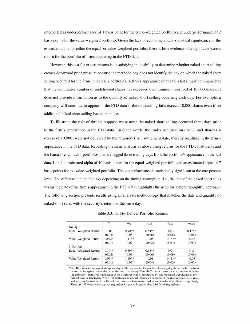
interpreted as underperformance of 1 basis point for the equal-weighted portfolio and underperformance of 2

basis points for the value-weighted portfolio. Given the lack of economic and/or statistical significance of the

estimated alpha for either the equal- or value-weighted portfolio, there is little evidence of a significant excess

return for the portfolio of firms appearing in the FTD data.

However, this test for excess returns is unsatisfying in its ability to determine whether naked short selling

creates downward price pressure because the methodology does not identify the day on which the naked short

selling occurred for the firms in the daily portfolios. A firm’s appearance on the fails list simply communicates

that the cumulative number of undelivered shares has exceeded the minimum threshold of 10,000 shares. It

does not provide information as to the quantity of naked short selling occurring each day. For example, a

company will continue to appear in the FTD data if the outstanding fails exceed 10,000 shares even if no

additional naked short selling has taken place.

To illustrate the role of timing, suppose we assume the naked short selling occurred three days prior

to the firm’s appearance in the FTD data. In other words, the trades occurred on date T and shares (in

excess of 10,000) were not delivered by the required T + 3 settlement date, thereby resulting in the firm’s

appearance in the FTD data. Repeating the same analysis as above using returns for the FTD constituents and

the Fama-French factor portfolios that are lagged three trading days from the portfolio’s appearance in the fail

data, I find an estimated alpha of 10 basis points for the equal-weighted portfolio and an estimated alpha of 7

basis points for the value-weighted portfolio. This outperformance is statistically significant at the one-percent

level. The difference in the findings depending on the timing assumption (i.e., the date of the naked short sales

versus the date of the firm’s appearance in the FTD data) highlights the need for a more thoughtful approach.

The following section presents results using an analysis methodology that matches the date and quantity of

naked short sales with the security’s return on the same day.

Table 3.3: Fail-to-Deliver Portfolio Returns

α Rm Rsmb Rhml RmomNo lagEqual-Weighted Return -0.01 0.90** 0.54** 0.03 0.17**

(0.03) (0.03) (0.06) (0.08) (0.06)Value-Weighted Return -0.02* 1.11** -0.05 -0.15** -0.02

(0.01) (0.02) (0.03) (0.04) (0.03)3-Day lagEqual-Weighted Return 0.10** 0.89** 0.58** 0.04 0.11

(0.02) (0.03) (0.06) (0.09) (0.06)Value-Weighted Return 0.07** 1.10** -0.01 -0.18** -0.03

(0.01) (0.02) (0.04) (0.05) (0.03)

Note: The estimates are reported as percentages. The lag denotes the number of trading days between the portfolioreturn and its appearance in the fail to deliver data. Newey-West HAC standard errors are in parentheses belowthe estimates. Statistical significance at the 5 percent level is denoted by (*) and statistical significance at the 1percent level is denoted by (**). FTD portfolio and market returns are in excess of the risk-free rate. Rsmb, Rhml ,and Rmom are the returns of the Fama-French size, book-to-market, and momentum factor portfolios, respectively.There are 193 observations and the regression R-squared is greater than 0.90 for all regressions.

78

3.6 Portfolio Returns by Decile

In this section, I evaluate the relationship between naked short sales and asset returns by forming daily

portfolios based on the amount of naked short selling. I estimate the excess returns of these portfolios to

determine whether portfolios of stocks subject to naked short selling underperform on the day the naked

short sales occur. This strategy permits two ways to assess return performance. The first is to look at the

excess returns of each portfolio in isolation after controlling for the Fama-French factors and momentum (i.e,

performance after controlling for factors known to predict returns). The second is to compare excess returns

across portfolios of stocks that experience different degrees of naked short selling.

Using the SEC’s reports of cumulative fails to deliver, I calculate the change in the number of fails between

consecutive trading days (including the change across weekends from Friday to Monday and across holidays).

This gives the net number of naked short sales (new fails less closed fail positions) that occurred on each

trading day for the stocks included in the FTD data.12 I form daily portfolios based on companies’ decile

rankings for the change in the number of fails. For example, the Decile 1 portfolio includes the stocks with the

largest decrease in the number of fails and the Decile 10 portfolio includes the stocks with the largest increase

in the number of fails.

Table 3.4 reports the average number of fails and the average change in the number of fails for each of the

deciles. The mean change in fails ranges from -150,978 shares for Decile 1 to 154,111 shares for Decile 10. A

potential concern arises if companies appearing multiple times in the FTD data are always assigned to the same

decile. The returns for the decile portfolios may then reflect firm characteristics rather than effects attributable

to naked short selling. This is not the case. Rather, there is substantial turnover among the constituents of each

decile.13

For each of the decile portfolios, I calculate the equal- and value-weighted returns three trading days prior

to the FTD settlement report. As mentioned earlier, the failure to deliver a share is formally considered a “fail"

if the share is not delivered by three trading days following the actual trade date. Therefore, if I am interested

in the relationship between naked short sales and stock returns, I should consider the portfolio returns on the

trading day when the naked short selling occurred, not on the date when those trades settled.

12Note that I only calculate the change in the number of fails if the firm appears in the fail data on consecutive days. This ensures that Icorrectly match the change in fails with the corresponding returns on the day when the trading occurred.

13For example, for the deciles formed based on the ratio of the change in fails to trading volume, the average standard deviation ofassigned deciles across firms is 2.75.

79

Table 3.4: Statistics by Decile

Decile Observations Mean Fails Mean Change in Fails1 43,205 272,418 -150,9782 43,302 134,761 -14,6043 43,309 92,788 -3,9724 39,781 78,853 -7805 52,953 90,876 -86 38,586 86,942 387 42,507 72,977 1,0938 43,081 94,632 4,9289 43,094 151,321 16,45910 43,100 441,595 154,111

Note: Deciles are formed based on the change in the number of fails betweenconsecutive trading days. In the case of a tie, the observation is randomlyassigned to the higher or lower decile. For each trading day, there areapproximately 226 companies in each decile.

Using these portfolio returns, I estimate the following specification for each of the deciles:

Rd,t = α +β1 ∗Rm,t +β2 ∗Rsmb,t +β3 ∗Rhml,t +β4 ∗Rmom,t + εt (3.2)

where Rd,t is the portfolio return for decile d less the risk-free interest rate on date t, Rm,t is the market

return less the risk-free interest rate, and Rsmb,t , Rhml,t , and Rmom,t are the returns of the Fama-French size,

book-to-market, and momentum factor portfolios, respectively. I report the resulting estimates for each of the

deciles in Tables 3.5 and 3.6.

The results for the equal-weighted portfolios are fairly striking. The excess returns progress from negative

values for the lower deciles to positive values for the higher deciles and nearly all of these estimates are

statistically significant at the 1 percent level. In other words, portfolios of stocks with large decreases in fails

to deliver underperformed and portfolios of stocks with large increases in fails to deliver outperformed. For the

value-weighted portfolios, the pattern of excess returns is less dramatic, but the estimated alphas do roughly

increase across deciles. The deciles containing firms with the largest increases in failures to deliver (Deciles

7-10) experience positive and statistically significant excess returns ranging from 9 to 18 basis points. There is

no evidence that firms with higher levels of naked short selling (as proxied by large increases in the number of

fails) experience negative excess returns. Rather, these firms exhibit positive returns that are both economically

and statistically significant.

Arguably, the relevant metric is not simply the change in the number of fails, but rather the change in the

number of fails relative to daily trading volume. Stocks that experience a larger number of naked short sales

as a fraction of trading volume may have negative excess returns as the additional short sales exert greater

downward pressure on prices. Table 3.7 provides descriptive statistics for decile portfolios formed according

80

Table 3.5: Equal-Weighted Decile Returns

Decile α Rm Rsmb Rhml Rmom1 -0.13* 1.03** 0.60** 0.03 0.24*

(0.05) (0.06) (0.09) (0.11) (0.09)2 -0.22** 0.89** 0.61** 0.05 0.17*

(0.04) (0.05) (0.08) (0.11) (0.07)3 -0.25** 0.79** 0.43** 0.12 0.17*

(0.04) (0.06) (0.07) (0.10) (0.07)4 -0.14** 0.55** 0.34 -0.03 0.19*

(0.04) (0.05) (0.09) (0.11) (0.08)5 -0.20** 0.67** 0.40** 0.29 0.10

(0.08) (0.17) (0.16) (0.29) (0.13)6 -0.12 0.51** 0.49** 0.42 0.19

(0.07) (0.11) (0.16) (0.23) (0.18)7 0.12** 0.73** 0.34** 0.13 0.07

(0.03) (0.05) (0.06) (0.09) (0.07)8 0.15** 0.79** 0.60** 0.05 0.14

(0.04) (0.05) (0.08) (0.12) (0.09)9 0.23** 0.86** 0.76** -0.06 0.31**

(0.05) (0.07) (0.10) (0.13) (0.09)10 0.44** 1.05** 0.71** -0.14 0.17

(0.09) (0.10) (0.16) (0.22) (0.16)

Note: Deciles are formed based on the change in the number of fails between consecutive tradingdays. The estimates are reported as percentages. Newey-West HAC standard errors are in parenthe-ses below the estimates. Statistical significance at the 5 percent level is denoted by (*) and statisticalsignificance at the 1 percent level is denoted by (**). Portfolio returns are equal-weighted and boththe portfolio and market returns are returns in excess of the risk-free rate. Rsmb, Rhml , and Rmom arethe returns of the Fama French size, book-to-market, and momentum factor portfolios, respectively.There are 192 observations for each decile.

Table 3.6: Value-Weighted Decile Returns

Decile α Rm Rsmb Rhml Rmom1 -0.011 1.00** 0.15 -0.30** 0.11

(0.03) (0.06) (0.09) (0.11) (0.07)2 -0.072* 1.11** 0.10 0.05 -0.12

(0.03) (0.06) (0.11) (0.15) (0.10)3 -0.097** 1.11** -0.06 -0.07 0.08

(0.04) (0.08) (0.12) (0.14) (0.09)4 0.019 0.82** 0.23* -0.01 0.02

(0.04) (0.06) (0.09) (0.12) (0.09)5 0.028 0.84** 0.24 0.03 0.03

(0.06) (0.11) (0.14) (0.18) (0.14)6 -0.101 0.71** 0.23 -0.03 0.23

(0.07) (0.12) (0.22) (0.24) (0.19)7 0.091** 0.99** 0.09 0.14 -0.06

(0.03) (0.08) (0.11) (0.12) (0.08)8 0.065 1.09** 0.18 0.16 -0.10

(0.04) (0.08) (0.11) (0.12) (0.10)9 0.180** 1.14** -0.06 -0.41** 0.22*

(0.03) (0.07) (0.09) (0.13) (0.10)10 0.141** 1.24** -0.01 -0.24 -0.07

(0.04) (0.08) (0.12) (0.13) (0.10)

Note: Deciles are formed based on the change in the number of fails between consecutive trading days.The estimates are reported as percentages. Newey-West HAC standard errors are in parenthesesbelow the estimates. Statistical significance at the 5 percent level is denoted by (*) and statisticalsignificance at the 1 percent level is denoted by (**). Portfolio returns are value-weighted and boththe portfolio and market returns are returns in excess of the risk-free rate. Rsmb, Rhml , and Rmom arethe returns of the Fama French size, book-to-market, and momentum factor portfolios, respectively.There are 192 observations for each decile.

81

to this measure. Decile 1 contains stocks with the smallest (i.e. negative) ratio of the change in fails to trading

volume and Decile 10 contains stocks with the largest ratio. I estimate Equation 3.2 for each of the deciles and

report the results in Tables 3.8 and 3.9.

Using equal-weighted portfolios, Deciles 1 through 5 underperform by a range of 7 to 25 basis points.

Deciles 6 through 9 outperform by a range of 13 to 40 basis points and these alphas are statistically significant

at the one percent level. Given the relatively small transaction costs associated with exchange-traded stocks and

the fact that the estimated alphas are daily returns, the economic significance of the excess returns accumulates

to a substantial magnitude over longer time horizons. For the value-weighted portfolios, Deciles 6 through 8

exhibit outperformance, but other than a negative estimated alpha for Decile 2, the estimated alphas for the

other deciles are not statistically significant. Again, these results do not support the claim that stocks subject to

naked short selling experience negative excess returns due to selling pressure.

A logical interpretation of the estimation results is that naked short sellers target stocks that outperform

during the trading day and then cover these fail positions (i.e., deliver shares to offset an existing fail) on

days when the stocks underperform. In following this strategy, naked short sellers are able to profit from

declines in stock prices without incurring the cost of borrowing shares.14 The stronger economic and statistical

significance of the equal-weighted portfolios’ excess returns relative to those of the value-weighted portfolios

suggests this trading behavior is particularly focused on firms with smaller market capitalizations.15

In order to look at these patterns more closely, I restrict the data sample to those firms with a non-negative

change in fails to deliver. In order to close a fail position, the short seller must either borrow a share from

an existing owner or purchase a share in the market. When the share is delivered to the clearing house, the

outstanding fail is eliminated. The data does not distinguish between fail positions that are closed using

borrowed shares and those that are closed using purchased shares. If the shares are borrowed, there is no

trading activity to which we can attribute excess returns. In addition, the primary objective of this analysis is

to determine whether there is evidence of selling pressure attributable to naked shorting. Removing firms with

negative net changes in fails allows me to focus exclusively on stocks subject to naked short selling on each

trading day.

Table 3.10 presents statistics for deciles formed based on the ratio of the change in the number of fails

to daily trading volume where the change in fails is greater than or equal to zero. The mean change in fails

ranges from 1,023 shares for Decile 1 to 70,039 shares for Decile 10. Tables 3.11 and 3.12 report results from

14Boni(2006) provides evidence that market makers strategically fail to deliver shares when borrowing costs (proxied by marketcapitalization, book-to-market ratio, and institutional ownership) are high. In addition to the standard stock borrowing costs measuredby the rebate rate, a naked short seller also avoids the requirement to pay dividends to the stock lender.

15While the results are stronger for the equal-weighted portfolios, recall that the CRSP sample covers relatively larger companies thattrade on NYSE, AMEX and Nasdaq. In addition, the summary statistics illustrate that the companies appearing in the FTD data are onaverage larger than the companies in the CRSP data.

82

the estimation of Equation 3.2 for each of the decile portfolios. For the equal-weighted portfolios, the lower

and middle deciles (Deciles 2 through 7) have positive excess returns that are economically and statistically

significant (ranging from 19 to 40 basis points). The results are similar, although smaller in magnitude, for the

value-weighted portfolios.

Once again, there is no evidence that stocks subject to naked short selling experience negative excess

returns. However, the pattern of estimated alphas across deciles is interesting. As suggested earlier, naked short

sellers appear to target stocks that outperform during the trading day. If so, we would expect all of the deciles

to exhibit outperformance. This is not the case for the highest deciles in either the equal- or value-weighted

regressions and is especially apparent when I restrict the data sample to those firms with a non-negative change

in fails. One explanation for this finding is that the amount of naked shorting of stocks in the highest deciles is

substantial enough to offset their positive excess returns. In other words, the naked shorting generates selling

pressure that depresses prices.

Table 3.7: Statistics by Decile – Change in Fails Relative to Volume

Decile Observations Mean Mean (Change Mean (Change in Std Dev (Change inFails in Fails) Fails / Volume) Fails / Volume)

1 16,784 159,326 -85,764 -1.27 8.732 16,878 151,833 -47,046 -0.13 0.053 16,890 120,954 -32,537 -0.05 0.024 16,880 102,940 -21,598 -0.02 0.015 16,903 74,334 -5,439 -0.002 0.0046 16,870 87,183 10,184 0.004 0.0057 16,875 129,609 25,746 0.02 0.018 16,795 161,541 37,404 0.05 0.029 17,033 191,255 49,193 0.12 0.0510 16,758 199,303 64,023 0.63 4.52

Note: Deciles are formed based on the ratio of the change in the number of fails to daily trading volume. In the caseof a tie, the observation is randomly assigned to the higher or lower decile. Observations with trading volumegreater than the 99th percentile are dropped. For each trading day, there are approximately 88 companies in eachdecile.

83

Table 3.8: Equal-Weighted Decile Returns – Change in Fails Relative toVolume

Decile α Rm Rsmb Rhml Rmom1 -0.225** 0.64** 0.38** 0.25** 0.01

(0.03) (0.05) (0.08) (0.09) (0.07)2 -0.229** 0.80** 0.38** 0.12 0.25**

(0.05) (0.07) (0.09) (0.13) (0.09)3 -0.256** 0.86** 0.67** 0.16 0.19

(0.05) (0.06) (0.09) (0.11) (0.10)4 -0.134* 0.94** 0.53** -0.13 0.36**

(0.05) (0.07) (0.11) (0.14) (0.10)5 -0.076* 0.91** 0.56** -0.22 0.16

(0.04) (0.05) (0.09) (0.11) (0.08)6 0.220** 0.93** 0.66** -0.27 0.27*

(0.05) (0.08) (0.13) (0.15) (0.11)7 0.404** 1.05** 0.76** -0.05 0.18

(0.07) (0.09) (0.13) (0.20) (0.17)8 0.314** 0.78** 0.69** -0.03 0.17

(0.06) (0.08) (0.12) (0.15) (0.11)9 0.132** 0.75** 0.58** 0.17 0.15

(0.05) (0.06) (0.10) (0.13) (0.10)10 0.058 0.65** 0.31** 0.19 0.21*

(0.04) (0.05) (0.08) (0.10) (0.08)

Note: Deciles are formed based on the ratio of the change in the number of fails to daily trading volume.The estimates are reported as percentages. Newey-West HAC standard errors are in parentheses.Statistical significance at the 5 percent level is denoted by (*) and statistical significance at the 1percent level is denoted by (**). Portfolio returns are equal-weighted and both the portfolio andmarket returns are returns in excess of the risk-free rate. Rsmb, Rhml , and Rmom are the returns ofthe Fama French size, book-to-market, and momentum factor portfolios, respectively. There are 192observations for each decile.

Table 3.9: Value-Weighted Decile Returns – Change in Fails Relative toVolume

Decile α Rm Rsmb Rhml Rmom1 -0.075 0.87** 0.21 0.21 -0.07

(0.04) (0.07) (0.11) (0.14) (0.13)2 -0.079* 0.97** 0.25** 0.20 0.04

(0.04) (0.06) (0.08) (0.12) (0.08)3 -0.057 0.92** 0.29** 0.11 0.07

(0.03) (0.07) (0.11) (0.13) (0.10)4 0.015 1.10** 0.08 -0.03 0.07

(0.03) (0.07) (0.10) (0.11) (0.08)5 -0.081 1.06** 0.16 -0.41** -0.07

(0.04) (0.07) (0.13) (0.13) (0.09)6 0.141** 1.15** -0.03 -0.34** 0.01

(0.03) (0.06) (0.09) (0.10) (0.09)7 0.220** 1.22** -0.04 -0.09 0.04

(0.05) (0.11) (0.12) (0.17) (0.12)8 0.132* 1.16** 0.09 0.06 0.16

(0.06) (0.12) (0.16) (0.20) (0.14)9 0.049 0.94** 0.47** 0.37* 0.16

(0.05) (0.08) (0.13) (0.16) (0.13)10 0.005 0.85** 0.23* 0.24 0.10

(0.04) (0.07) (0.11) (0.13) (0.10)

Note: Deciles are formed based on the ratio of the change in the number of fails to daily trading volume.The estimates are reported as percentages. Newey-West HAC standard errors are in parentheses.Statistical significance at the 5 percent level is denoted by (*) and statistical significance at the 1percent level is denoted by (**). Portfolio returns are value-weighted and both the portfolio andmarket returns are returns in excess of the risk-free rate. Rsmb, Rhml , and Rmom are the returns ofthe Fama French size, book-to-market, and momentum factor portfolios, respectively. There are 192observations for each decile.

84

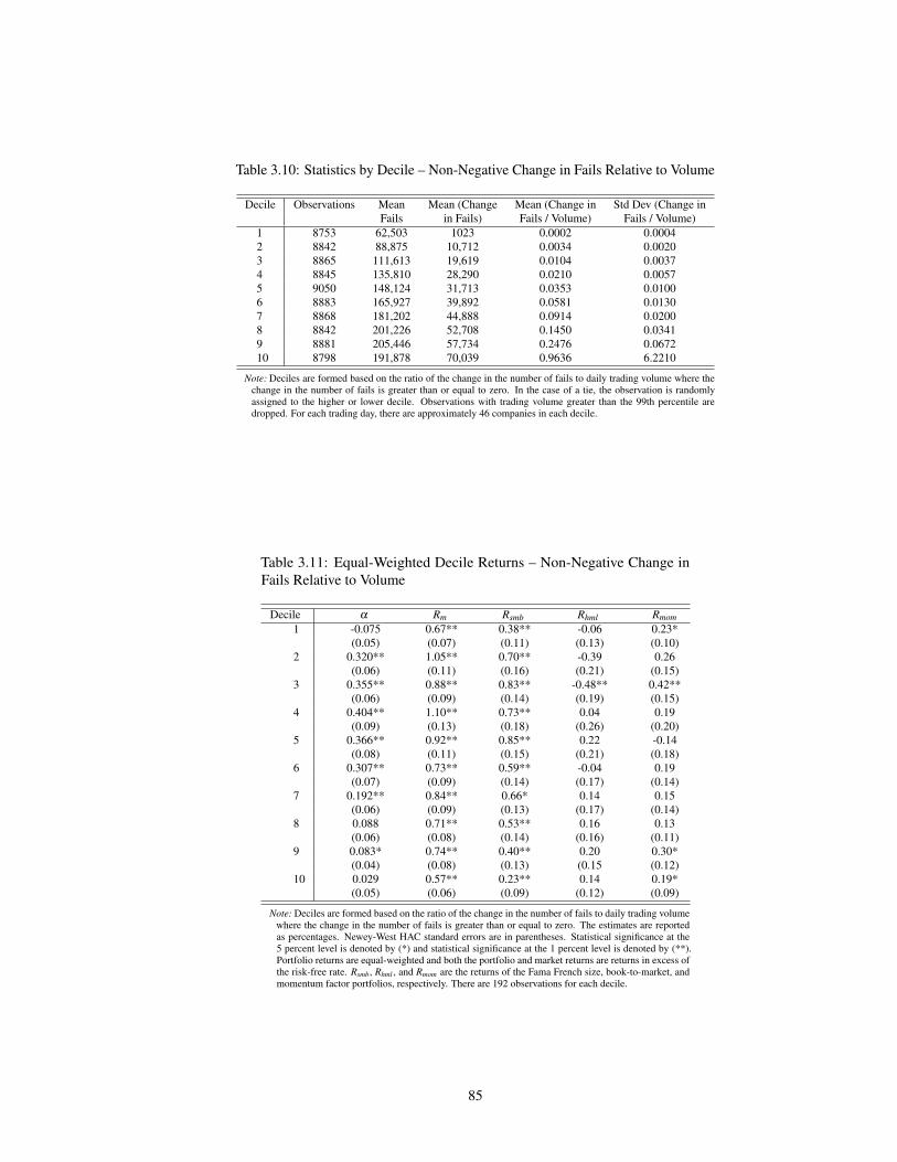
Table 3.10: Statistics by Decile – Non-Negative Change in Fails Relative to Volume

Decile Observations Mean Mean (Change Mean (Change in Std Dev (Change inFails in Fails) Fails / Volume) Fails / Volume)

1 8753 62,503 1023 0.0002 0.00042 8842 88,875 10,712 0.0034 0.00203 8865 111,613 19,619 0.0104 0.00374 8845 135,810 28,290 0.0210 0.00575 9050 148,124 31,713 0.0353 0.01006 8883 165,927 39,892 0.0581 0.01307 8868 181,202 44,888 0.0914 0.02008 8842 201,226 52,708 0.1450 0.03419 8881 205,446 57,734 0.2476 0.067210 8798 191,878 70,039 0.9636 6.2210

Note: Deciles are formed based on the ratio of the change in the number of fails to daily trading volume where thechange in the number of fails is greater than or equal to zero. In the case of a tie, the observation is randomlyassigned to the higher or lower decile. Observations with trading volume greater than the 99th percentile aredropped. For each trading day, there are approximately 46 companies in each decile.

Table 3.11: Equal-Weighted Decile Returns – Non-Negative Change inFails Relative to Volume

Decile α Rm Rsmb Rhml Rmom1 -0.075 0.67** 0.38** -0.06 0.23*

(0.05) (0.07) (0.11) (0.13) (0.10)2 0.320** 1.05** 0.70** -0.39 0.26

(0.06) (0.11) (0.16) (0.21) (0.15)3 0.355** 0.88** 0.83** -0.48** 0.42**

(0.06) (0.09) (0.14) (0.19) (0.15)4 0.404** 1.10** 0.73** 0.04 0.19

(0.09) (0.13) (0.18) (0.26) (0.20)5 0.366** 0.92** 0.85** 0.22 -0.14

(0.08) (0.11) (0.15) (0.21) (0.18)6 0.307** 0.73** 0.59** -0.04 0.19

(0.07) (0.09) (0.14) (0.17) (0.14)7 0.192** 0.84** 0.66* 0.14 0.15

(0.06) (0.09) (0.13) (0.17) (0.14)8 0.088 0.71** 0.53** 0.16 0.13

(0.06) (0.08) (0.14) (0.16) (0.11)9 0.083* 0.74** 0.40** 0.20 0.30*

(0.04) (0.08) (0.13) (0.15 (0.12)10 0.029 0.57** 0.23** 0.14 0.19*

(0.05) (0.06) (0.09) (0.12) (0.09)

Note: Deciles are formed based on the ratio of the change in the number of fails to daily trading volumewhere the change in the number of fails is greater than or equal to zero. The estimates are reportedas percentages. Newey-West HAC standard errors are in parentheses. Statistical significance at the5 percent level is denoted by (*) and statistical significance at the 1 percent level is denoted by (**).Portfolio returns are equal-weighted and both the portfolio and market returns are returns in excess ofthe risk-free rate. Rsmb, Rhml , and Rmom are the returns of the Fama French size, book-to-market, andmomentum factor portfolios, respectively. There are 192 observations for each decile.

85

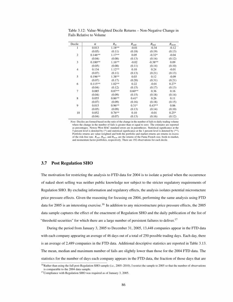
Table 3.12: Value-Weighted Decile Returns – Non-Negative Change inFails Relative to Volume

Decile α Rm Rsmb Rhml Rmom1 0.013 1.18** -0.01 -0.34 -0.12

(0.05) (0.11) (0.18) (0.19) (0.13)2 0.146** 1.17** 0.05 -0.32* -0.04

(0.04) (0.08) (0.13) (0.14) (0.12)3 0.180** 1.16** -0.02 -0.38** 0.09

(0.05) (0.08) (0.11) (0.14) (0.10)4 0.134 1.12** 0.10 0.24 -0.01

(0.07) (0.11) (0.13) (0.21) (0.13)5 0.196** 1.38** 0.03 0.12 -0.09

(0.07) (0.17) (0.20) (0.31) (0.21)6 0.115** 1.02** 0.22 -0.01 0.27*

(0.04) (0.12) (0.15) (0.17) (0.13)7 0.085 0.87** 0.60** 0.36 0.16

(0.04) (0.09) (0.15) (0.18) (0.14)8 0.055 0.86** 0.41* 0.26 0.11

(0.07) (0.09) (0.16) (0.18) (0.15)9 0.015 0.96** 0.31* 0.43** 0.06

(0.05) (0.09) (0.13) (0.14) (0.10)10 0.052 0.76** 0.10 -0.01 0.25*

(0.04) (0.07) (0.13) (0.16) (0.12)

Note: Deciles are formed based on the ratio of the change in the number of fails to daily trading volumewhere the change in the number of fails is greater than or equal to zero. The estimates are reportedas percentages. Newey-West HAC standard errors are in parentheses. Statistical significance at the5 percent level is denoted by (*) and statistical significance at the 1 percent level is denoted by (**).Portfolio returns are value-weighted and both the portfolio and market returns are returns in excessof the risk-free rate. Rsmb, Rhml , and Rmom are the returns of the Fama French size, book-to-market,and momentum factor portfolios, respectively. There are 192 observations for each decile.

3.7 Post Regulation SHO

The motivation for restricting the analysis to FTD data for 2004 is to isolate a period when the occurrence

of naked short selling was neither public knowledge nor subject to the stricter regulatory requirements of

Regulation SHO. By excluding information and regulatory effects, the analysis isolates potential microstucture

price pressure effects. Given the reasoning for focusing on 2004, performing the same analysis using FTD

data for 2005 is an interesting exercise.16 In addition to any microstructure price pressure effects, the 2005

data sample captures the effect of the enactment of Regulation SHO and the daily publication of the list of

“threshold securities" for which there are a large number of persistent failures to deliver.17

During the period from January 3, 2005 to December 31, 2005, 13,448 companies appear in the FTD data

with each company appearing an average of 46 days out of a total of 250 possible trading days. Each day, there

is an average of 2,489 companies in the FTD data. Additional descriptive statistics are reported in Table 3.13.

The mean, median and maximum number of fails are slightly lower than those for the 2004 FTD data. The

statistics for the number of days each company appears in the FTD data, the fraction of those days that are

16Rather than using the full post-Regulation SHO sample (i.e., 2005–2010), I restrict the sample to 2005 so that the number of observationsis comparable to the 2004 data sample.

17Compliance with Regulation SHO was required as of January 3, 2005.

86

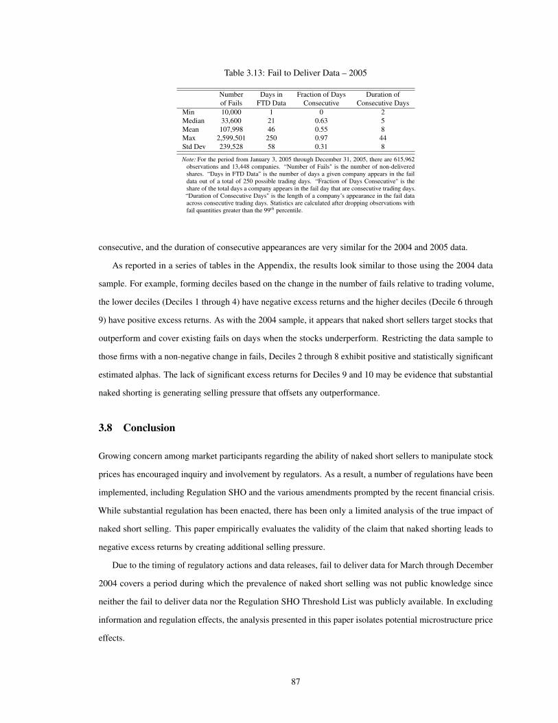
Table 3.13: Fail to Deliver Data – 2005

Number Days in Fraction of Days Duration ofof Fails FTD Data Consecutive Consecutive Days

Min 10,000 1 0 2Median 33,600 21 0.63 5Mean 107,998 46 0.55 8Max 2,599,501 250 0.97 44Std Dev 239,528 58 0.31 8

Note: For the period from January 3, 2005 through December 31, 2005, there are 615,962observations and 13,448 companies. “Number of Fails" is the number of non-deliveredshares. “Days in FTD Data" is the number of days a given company appears in the faildata out of a total of 250 possible trading days. “Fraction of Days Consecutive" is theshare of the total days a company appears in the fail day that are consecutive trading days.“Duration of Consecutive Days" is the length of a company’s appearance in the fail dataacross consecutive trading days. Statistics are calculated after dropping observations withfail quantities greater than the 99th percentile.

consecutive, and the duration of consecutive appearances are very similar for the 2004 and 2005 data.

As reported in a series of tables in the Appendix, the results look similar to those using the 2004 data

sample. For example, forming deciles based on the change in the number of fails relative to trading volume,

the lower deciles (Deciles 1 through 4) have negative excess returns and the higher deciles (Decile 6 through

9) have positive excess returns. As with the 2004 sample, it appears that naked short sellers target stocks that

outperform and cover existing fails on days when the stocks underperform. Restricting the data sample to

those firms with a non-negative change in fails, Deciles 2 through 8 exhibit positive and statistically significant

estimated alphas. The lack of significant excess returns for Deciles 9 and 10 may be evidence that substantial

naked shorting is generating selling pressure that offsets any outperformance.

3.8 Conclusion

Growing concern among market participants regarding the ability of naked short sellers to manipulate stock

prices has encouraged inquiry and involvement by regulators. As a result, a number of regulations have been

implemented, including Regulation SHO and the various amendments prompted by the recent financial crisis.

While substantial regulation has been enacted, there has been only a limited analysis of the true impact of

naked short selling. This paper empirically evaluates the validity of the claim that naked shorting leads to

negative excess returns by creating additional selling pressure.

Due to the timing of regulatory actions and data releases, fail to deliver data for March through December

2004 covers a period during which the prevalence of naked short selling was not public knowledge since

neither the fail to deliver data nor the Regulation SHO Threshold List was publicly available. In excluding

information and regulation effects, the analysis presented in this paper isolates potential microstructure price

effects.

87

Using a methodology that constructs daily portfolios according to the quantity of naked short selling, I

find no evidence that stocks subject to naked short selling experience negative excess returns. Rather, I find

evidence that these stocks often outperform on the day the trades occur. Naked short sellers appear to target

stocks that outperform during the trading day and cover existing fails on days when the stocks underperform.

In following this strategy, naked short sellers are able to profit from declines in stock prices without incurring

the cost of borrowing shares. The absence of outperformance for the highest decile portfolios suggests that

significant amounts of naked short selling may offset positive excess returns through microstructure price

pressure.

The motivation for limiting the data sample to 2004 was concern that data for later time periods would

conflate microstructure selling pressure effects with information and regulation effects. However, the results

are very similar using fail to deliver data for the year following the implementation of Regulation SHO. In

particular, portfolios of firms subject to moderate amounts of naked short selling continue to experience

significant positive excess returns while portfolios of firms subject to the greatest amount of naked selling do

not have economically or statistically significant excess returns.

The reputation of naked short selling as a manipulative trading activity among company executives and

the popular press has undoubtedly placed pressure on regulators to take action. Nonetheless, regulation of

financial market activity should ideally respond to problems evidenced by an analysis of the relevant data

rather than simply reacting to market sentiment. The analysis presented in this paper finds that naked short

selling is not systematically associated with negative excess returns. However, there is evidence that naked

short sellers strategically time their sales to capture profits without the eroding effect of borrowing costs. Given

the undesirability of trading strategies that circumvent market rules and standards, and the observation that

significant amounts of naked shorting may be offsetting positive returns, further regulation with the aim of

eliminating naked short selling may be warranted.

88

3.9 Appendix

3.9.1 Covered versus Naked Short Selling

It is important to make the distinction between covered and naked short selling clear. Suppose an investor has

a negative view of future returns for a particular stock but does not currently own shares of the stock. In a

covered short sale, the investor is able to effect a sale by borrowing the share from a current owner of the stock

and then selling this share to a buyer in the marketplace. If the share price goes down, the investor makes a

profit because he repurchases the share at a lower price when he returns the share to its original owner. During

the share borrowing period, the investor gives the lending owner collateral equivalent to 102–105 percent of

the share price and, in return, receives interest on this collateral. The interest received is known as the “rebate

rate". A stock with a lower rebate rate is one which is considered more expensive to borrow. In the extreme,

the rebate rate may be negative, meaning the investor does not receive interest on his collateral, but instead

makes additional payments to the lender.

In the case of a naked short sale, the investor does not locate a share to borrow. Instead, the investor enters

into a short sale in the marketplace, but fails to deliver a share to the buyer by the required T+3 settlement

date (three days following the trade date).18 Some failures to deliver occur as the result of legitimate trading

practices (i.e. market making) or settlement errors. Outside of these situations, an intentional failure to deliver

shares to the buyer is considered manipulative. Why might a market participant intentionally fail to deliver a

share? Based on an analysis of fail to deliver data, Boni (2006) concludes that “market makers strategically

fail to deliver shares when borrowing costs are high." In other words, when the rebate rate on a stock is low,

there is an incentive to not borrow the share.

3.9.2 Regulation SHO

Regulation SHO became effective on September 7, 2004 and required market compliance beginning January

3, 2005. It was designed to achieve several objectives: (1) Establish uniform stock location and delivery

requirements in order to address problems associated with failures to deliver, including potential abusive naked

short selling; (2) Create uniform marking requirements for sales of all equity securities (i.e. long, short or

short-exempt); and (3) Temporarily suspend short sale tests for a pilot group of securities in order to evaluate

the overall effectiveness and necessity of such restrictions.

Regulation SHO required the daily publication of lists of Threshold securities ("Regulation SHO Threshold

List") by securities associations or exchanges (i.e., SROs), starting on January 7, 2005. Threshold securities

18The SEC website (http://www.sec.gov/) is a good source for detailed information on the stock clearing process overseen by theDepository Trust & Clearing Corporation (DTCC) (http://www.dtcc.com/).

89

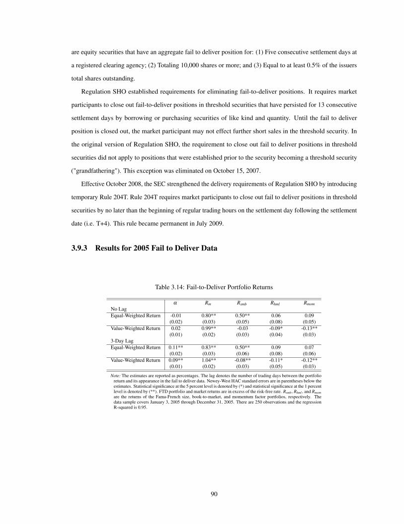
are equity securities that have an aggregate fail to deliver position for: (1) Five consecutive settlement days at

a registered clearing agency; (2) Totaling 10,000 shares or more; and (3) Equal to at least 0.5% of the issuers

total shares outstanding.

Regulation SHO established requirements for eliminating fail-to-deliver positions. It requires market

participants to close out fail-to-deliver positions in threshold securities that have persisted for 13 consecutive

settlement days by borrowing or purchasing securities of like kind and quantity. Until the fail to deliver

position is closed out, the market participant may not effect further short sales in the threshold security. In

the original version of Regulation SHO, the requirement to close out fail to deliver positions in threshold

securities did not apply to positions that were established prior to the security becoming a threshold security

("grandfathering"). This exception was eliminated on October 15, 2007.

Effective October 2008, the SEC strengthened the delivery requirements of Regulation SHO by introducing

temporary Rule 204T. Rule 204T requires market participants to close out fail to deliver positions in threshold

securities by no later than the beginning of regular trading hours on the settlement day following the settlement

date (i.e. T+4). This rule became permanent in July 2009.

3.9.3 Results for 2005 Fail to Deliver Data

Table 3.14: Fail-to-Deliver Portfolio Returns

α Rm Rsmb Rhml RmomNo LagEqual-Weighted Return -0.01 0.80** 0.50** 0.06 0.09

(0.02) (0.03) (0.05) (0.08) (0.05)Value-Weighted Return 0.02 0.99** -0.03 -0.09* -0.13**

(0.01) (0.02) (0.03) (0.04) (0.03)3-Day LagEqual-Weighted Return 0.11** 0.83** 0.50** 0.09 0.07

(0.02) (0.03) (0.06) (0.08) (0.06)Value-Weighted Return 0.09** 1.04** -0.08** -0.11* -0.12**

(0.01) (0.02) (0.03) (0.05) (0.03)

Note: The estimates are reported as percentages. The lag denotes the number of trading days between the portfolioreturn and its appearance in the fail to deliver data. Newey-West HAC standard errors are in parentheses below theestimates. Statistical significance at the 5 percent level is denoted by (*) and statistical significance at the 1 percentlevel is denoted by (**). FTD portfolio and market returns are in excess of the risk-free rate. Rsmb, Rhml , and Rmomare the returns of the Fama-French size, book-to-market, and momentum factor portfolios, respectively. Thedata sample covers January 3, 2005 through December 31, 2005. There are 250 observations and the regressionR-squared is 0.95.

90

Table 3.15: Statistics by Decile – Change in Fails Relative to Volume

Decile Observations Mean Mean (Change Mean (Change in Std Dev (Change inFails in Fails) Fails / Volume) Fails / Volume)

1 18,572 117,308 -83,885 -0.97 5.542 18,684 108,689 -48,012 -0.11 0.043 18,707 98,431 -32,474 -0.04 0.024 18,694 85,440 -20,457 -0.01 0.015 18,609 64,767 -4,974 -0.002 0.0036 18,780 73,829 8,945 0.003 0.0047 18,727 109,989 23,920 0.02 0.018 18,681 134,475 37,839 0.05 0.029 18,710 152,582 49,267 0.11 0.0410 18,597 170,219 66,834 0.50 2.48

Note: The data sample covers January 3, 2005 through December 31, 2005. Deciles are formed based on the ratio ofthe change in the number of fails to daily trading volume. In the case of a tie, the observation is randomly assignedto the higher or lower decile. Observations with trading volume greater than the 99th percentile are dropped.

Table 3.16: Equal-Weighted Decile Returns – Change in Fails Relative toVolume

Decile α Rm Rsmb Rhml Rmom1 -0.160** 0.59** 0.25** -0.14 0.10

(0.02) (0.04) (0.07) (0.12) (0.07)2 -0.238** 0.81** 0.40** 0.19 0.01

(0.02) (0.05) (0.08) (0.14) (0.09)3 -0.260** 0.82** 0.60** 0.12 0.01

(0.03) (0.05) (0.09) (0.16) (0.10)4 -0.149** 0.94** 0.66** 0.32 -0.05

(0.03) (0.06) (0.09) (0.18) (0.11)5 -0.019 0.82** 0.47** 0.03 0.06

(0.02) (0.05) (0.08) (0.15) (0.09)6 0.232** 0.78** 0.61** -0.03 0.16

(0.04) (0.06) (0.11) (0.19) (0.11)7 0.347** 0.93** 0.78** 0.13 0.01

(0.05) (0.08) (0.14) (0.24) (0.15)8 0.298** 0.82** 0.64** 0.02 0.09

(0.04) (0.08) (0.12) (0.23) (0.14)9 0.180** 0.65** 0.55** 0.22 0.06

(0.03) (0.06) (0.10) (0.18) (0.12)10 0.039 0.67** 0.36** 0.26* -0.05

(0.03) (0.06) (0.08) (0.13) (0.08)

Note: Deciles are formed based on the ratio of the change in the number of fails to daily tradingvolume. The estimates are reported as percentages. Newey-West HAC standard errors are in paren-theses. Statistical significance at the 5 percent level is denoted by (*) and statistical significance atthe 1 percent level is denoted by (**). Portfolio returns are equal-weighted and both the portfolioand market returns are returns in excess of the risk-free rate. Rsmb, Rhml , and Rmom are the returnsof the Fama French size, book-to-market, and momentum factor portfolios, respectively. The datasample covers January 3, 2005 through December 31, 2005. There are 239 observations for eachdecile.

91

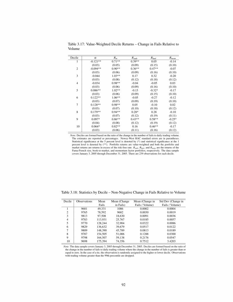
Table 3.17: Value-Weighted Decile Returns – Change in Fails Relative toVolume

Decile α Rm Rsmb Rhml Rmom1 -0.121** 0.71** 0.39** 0.05 -0.14

(0.03) (0.05) (0.09) (0.15) (0.10)2 -0.094** 0.90** 0.36** 0.47** -0.07

(0.03) (0.06) (0.09) (0.16) (0.10)3 -0.044 1.03** 0.17 0.32 -0.20

(0.03) (0.08) (0.12) (0.18) (0.12)4 -0.034 0.98** -0.04 -0.05 0.03

(0.03) (0.06) (0.09) (0.16) (0.10)5 0.086** 1.02** -0.15 -0.32* -0.17

(0.03) (0.06) (0.09) (0.15) (0.10)6 0.122** 1.06** -0.05 -0.27 -0.12

(0.03) (0.07) (0.09) (0.19) (0.10)7 0.128** 0.98** 0.05 -0.10 0.02

(0.03) (0.07) (0.10) (0.18) (0.12)8 0.179** 0.94** 0.28* 0.28 -0.10

(0.03) (0.07) (0.12) (0.19) (0.11)9 0.097* 0.86** 0.43** 0.58** -0.25*

(0.04) (0.08) (0.12) (0.19) (0.12)10 0.064* 0.82** 0.16 0.46** -0.17

(0.03) (0.06) (0.11) (0.16) (0.12)

Note: Deciles are formed based on the ratio of the change in the number of fails to daily trading volume.The estimates are reported as percentages. Newey-West HAC standard errors are in parentheses.Statistical significance at the 5 percent level is denoted by (*) and statistical significance at the 1percent level is denoted by (**). Portfolio returns are value-weighted and both the portfolio andmarket returns are returns in excess of the risk-free rate. Rsmb, Rhml , and Rmom are the returns of theFama-French size, book-to-market, and momentum factor portfolios, respectively. The data samplecovers January 3, 2005 through December 31, 2005. There are 239 observations for each decile.

Table 3.18: Statistics by Decile – Non-Negative Change in Fails Relative to Volume

Decile Observations Mean Mean (Change Mean (Change in Std Dev (Change inFails in Fails) Fails / Volume) Fails / Volume)

1 9681 49,331 1086 0.0002 0.00042 9765 78,592 9682 0.0030 0.00193 9813 97,508 18,630 0.0091 0.00364 9783 113,931 25,767 0.0185 0.00575 9770 128,244 32,904 0.0322 0.00866 9829 136,632 39,679 0.0517 0.01227 9809 148,390 45,789 0.0813 0.01898 9787 154,505 51,006 0.1288 0.03009 9798 164,507 59,138 0.2176 0.054710 9698 175,394 74,356 0.7512 3.4203

Note: The data sample covers January 3, 2005 through December 31, 2005. Deciles are formed based on the ratio ofthe change in the number of fails to daily trading volume where the change in the number of fails is greater than orequal to zero. In the case of a tie, the observation is randomly assigned to the higher or lower decile. Observationswith trading volume greater than the 99th percentile are dropped.

92

Table 3.19: Equal-Weighted Decile Returns – Non-Negative Change inFails Relative to Volume

Decile α Rm Rsmb Rhml Rmom1 0.004 0.70** 0.44** 0.13 0.01

(0.04) (0.08) (0.12) (0.20) (0.12)2 0.310** 0.81** 0.76** 0.05 0.07

(0.07) (0.08) (0.21) (0.32) (0.22)3 0.367** 0.95** 0.59** -0.05 0.26

(0.04) (0.11) (0.14) (0.25) (0.16)4 0.252** 0.92** 0.61** 0.02 0.03

(0.05) (0.09) (0.14) (0.23) (0.15)5 0.432** 0.72** 0.65** -0.32 0.32

(0.06) (0.11) (0.18) (0.33) (0.20)6 0.239** 0.92** 0.83** 0.34 -0.17

(0.05) (0.10) (0.14) (0.27) (0.17)7 0.226** 0.82** 0.46** 0.18 0.13

(0.04) (0.09) (0.13) (0.24) (0.17)8 0.163** 0.56** 0.60** 0.30 -0.03

(0.04) (0.06) (0.12) (0.21) (0.13)9 0.064 0.72** 0.42** 0.18 0.09

(0.04) (0.08) (0.10) (0.18) (0.11)10 0.013 0.58** 0.34** 0.43** -0.19*

(0.03) (0.06) (0.10) (0.15) (0.09)

Note: Deciles are formed based on the ratio of the change in the number of fails to daily trading volumewhere the change in the number of fails is greater than or equal to zero. The estimates are reportedas percentages. Newey-West HAC standard errors are in parentheses. Statistical significance at the5 percent level is denoted by (*) and statistical significance at the 1 percent level is denoted by (**).Portfolio returns are equal-weighted and both the portfolio and market returns are returns in excessof the risk-free rate. Rsmb, Rhml , and Rmom are the returns of the Fama-French size, book-to-market,and momentum factor portfolios, respectively. The data sample covers January 3, 2005 throughDecember 31, 2005. There are 239 observations for each decile.

Table 3.20: Value-Weighted Decile Returns – Non-Negative Change inFails Relative to Volume

Decile α Rm Rsmb Rhml Rmom1 0.088 0.93** 0.27* 0.18 -0.34

(0.05) (0.12) (0.14) (0.25) (0.13)2 0.097* 1.10** 0.03 -0.17 -0.12

(0.04) (0.07) (0.12) (0.17) (0.11)3 0.174** 1.07** 0.01 -0.20 0.02

(0.05) (0.11) (0.13) (0.22) (0.15)4 0.146** 1.01** 0.01 -0.22 -0.05

(0.05) (0.09) (0.14) (0.25) (0.17)5 0.132** 0.94** 0.28* 0.32 -0.20

(0.04) (0.09) (0.12) (0.24) (0.13)6 0.172** 0.96** 0.30** 0.36 0.01

(0.04) (0.09) (0.14) (0.25) (0.15)7 0.153** 0.96** 0.35* 0.51* -0.25

(0.04) (0.10) (0.14) (0.21) (0.14)8 0.107** 0.72** 0.53** 0.55* -0.17

(0.03) (0.09) (0.14) (0.23) (0.13)9 0.056 0.87** 0.18 0.57* -0.19

(0.04) (0.07) (0.11) (0.19) (0.14)10 0.062 0.73** 0.20 0.30 -0.08

(0.04) (0.07) (0.12) (0.17) (0.11)

Note: Deciles are formed based on the ratio of the change in the number of fails to daily tradingvolume where the change in the number of fails is greater than or equal to zero. The estimatesare reported as percentages. Newey-West HAC standard errors are in parentheses. Statisticalsignificance at the 5 percent level is denoted by (*) and statistical significance at the 1 percentlevel is denoted by (**). Portfolio returns are value-weighted and both the portfolio and marketreturns are returns in excess of the risk-free rate. Rsmb, Rhml , and Rmom are the returns of theFama-French size, book-to-market, and momentum factor portoflios, respectively. The data samplecovers January 3, 2005 through December 31, 2005. There are 239 observations for each decile.

93

Bibliography

Aitken, M. J., A. Frino, M. S. McCorry, and P. L. Swan. Short sales are almost instantaneously bad news:Evidence from the Australian Stock Exchange. Journal of Finance, 53(6), 2205–2223, 1998.

A.J. Senchack, J. and L. T. Starks. Short-sale restrictions and market reaction to short-interest announcements.Journal of Financial and Quantitative Analysis, 28, 177–194, 1993.

Allen, F. and D. Gale. Stock-price manipulation. Review of Financial Studies, 5(3), 503–529, 1992.

Angel, J. J., S. E. Christophe, and M. G. Ferri. A close look at short selling on Nasdaq. Financial AnalystsJournal, 59(6), 66–74, 2003.

Bechmann, K. L. Short sales, price pressure, and the stock price response to convertible bond calls. WorkingPaper, 2003.

Boehmer, E., C. M. James, and X. Zhang. Which shorts are informed? Working Paper, 2007.

Boni, L. Strategic delivery failures in U.S. equity markets. Journal of Financial Markets, 9, 1–26, 2006.

Boulton, T. J. and M. V. Braga-Alves. Naked short selling and market returns. Working Paper, 2009a.

Boulton, T. J. and M. V. Braga-Alves. The skinny on the 2008 naked short sale restrictions. Working Paper,2009b.

Chen, H. and V. Singal. Role of speculative short sales in price formation: The case of the weekend effect.Journal of Finance, 58, 685–705, 2003.

Christoffersen, S., C. Geczy, D. Musto, and A. Reed. How and why do investors trade votes, and what does itmean? Working Paper, 2004.

Coval, J. and E. Stafford. Asset fire sales (and purchases) in equity markets. Journal of Financial Economics,86, 479–512, 2007.

Culp, C. L. and J. Heaton. The economics of naked short selling. Securities & Exchange, 46–51, 2008.

Desai, H., K. Ramesh, S. R. Thiagarajan, and B. V. Balachandran. An investigation of the informational roleof short interest in the Nasdaq market. Journal of Finance, 57(5), 2263–2287, 2002.

Diamond, D. W. and R. E. Verrecchia. Constraints on short-selling and asset price adjustment to privateinformation. Journal of Financial Economics, 18, 277–311, 1987.

Diether, K. B., K. Lee, and I. M. Werner. Short-sale strategies and return predictability. Review of FinancialStudies, 2008.

Duffie, D., N. Garleanu, and L. H. Pedersen. Securities lending, shorting, and pricing. Journal of FinancialEconomics, 6, 307–339, 2002.

Easley, D. and M. O’Hara. Price, trade size, and information in securities markets. Journal of FinancialEconomics, 19, 69–90, 1987.

Evans, R. B., C. G. Geczy, D. K. Musto, and A. V. Reed. Failure is an option: Impediments to short sellingand options prices. Review of Financial Studies, 22(5), 1955–1980, 2009.

94

Finnerty, J. D. Short selling, death spiral convertibles, and the profitability of stock manipulation. WorkingPaper, 2005.

Fotak, V., V. Raman, and P. K. Yadav. Naked short selling: The emperor’s new clothes? Working Paper, 2009.

Glosten, L. and P. Milgrom. Bid, ask, and transaction prices in a specialist market with heterogeneouslyinformed traders. Journal of Financial Economics, 13, 71–100, 1985.

Karpoff, J. M. The relation between price changes and trading volume: A survey. Journal of Financial andQuantitative Analysis, 22, 109–126, 1987.

Kyle, A. S. Continuous auctions and insider trading. Econometrica, 53, 1315–1336, 1985.

Miller, E. M. Risk, uncertainty, and divergence of opinion. Journal of Finance, 32, 1151–1168, 1977.

Woolridge, J. R. and A. Dickinson. Short selling and common stock prices. Financial Analysts Journal, 50,20–28, 1994.

95