equilibrium chemical reaction of supersonic …
TRANSCRIPT

(_-.. ._-.a
NASA CONTRACTOR
REPORT
EQUILIBRIUM CHEMICAL REACTION OF SUPERSONIC HYDROGEN-AIR JETS (THE ALMA COMPUTER PROGRAM)
S. E@5obushi und D. B, S’alding
i Prepared by ‘, y .- _-’ .- :
FLUID MECHANICS 81 THERMAL SYSTEMS, INC. j _-. \ - “I’
Waverly, Ala. 36879 for Langley Research Center
NATIONAL AERONAUTICS AND SPACE ADMINISTRATION l WASHINGTON, D. C. l JANUARY 1977

I TECH LlBBARY KAFB, Nlld
1. Report No. 2. Government Accession No. 3. Recipient’s Catalog No. NASA CR-2725
4. Title and Subtitle 5. Report Date
EQIJILIBRIUM CHEMICAL REACTION OF SUPERSONIC HYDROGEN-AIR JETS ' January 1977 _
(THE ALMA COMPUTER PROGRAM) - 6. Performing Organization Code
7. Author(s)
S. Elghobashi and 0. B. Spalding
8. Performing Orgamzation Report No.
10. Work Unit No. 9. Performing Organization Name and Address
Concentration, Heat and Momentum Limited 86 Burlington Road, New Malden, England Subcontractor to: Fluid Mechanics & Thermal Systems,Inc. Route 2, Box 11, Waverly, AL 36879
505-05-41-02 11. Contract or Grant No.
NASl-13729 13. Type of Report and Period Covered
2. Sponsoring Agency Name and Address
National Aeronautics & Space Administration
Washington, DC 20546
5. Supplementary Notes
Langley technical monitor: John S. Evans, Jr.
Final report.
6. Abstract
The ALMA (Axi-symmetrical Lateral Momentum Analyser) program is concerned with the computation of 2-dimensional coaxial jets with large lateral pressure gradients. The jets
free or confined, laminar or turbulent, reacting or non-reacting. Reaction chemistry may be is equ ilibrium.
7. Key Words (Suggested by Authoris)) 16. Distribution Statement
Pressure gradient Coaxial jet Turbulent mixing Hydrogen-air Combustion
Unclassified - Unlimited
9. Security Classif. (of this report1
Unclassified
20. Security Classif. (of this page)
Unclassified
21. No. of Pw
57
22. Price*
$4.25
Subject Category 34
*For sale by the National Technical Information Service, Springfield, Virginia 22161

-

CONTENTS Page No.
1.
1.1 1.2 1.3
2.
2.1 2.2 2.3 2.3.1 1
2.3.2 2.4 2.4.1 2.4.2
THE MATHEMATICAL AND PHYSICAL ANALYSIS .......
Introduction .................... The mean-flow conservation equations ........
The turbulence model. ................ The turbulent viscosity ............... The concentration fluctuations .... ! ......
The combustion model. ................ Equations ...................... Solution procedure .................
' 3. THE NUMERICAL SOLUTION PROCEDURE .......... 10
3.1 3.2 3.3 3.3.1 3.3.2 3.3.3 3.4 3.5
Introduction .................... T'he finite-difference grid ............. The formulation of the solution algorithm ......
The Patankar-Spalding procedure ........... The relation between v and p ............ The pressure correction procedure (SIMPLE). .....
Conditions at the E-boundary in supersonic flow ... The basic solution steps ..............
10 11 11 12 13 14 18 19
4. DISCUSSION OF SAMPLE PREDICTIONS ..........
The jet surrounding a centre-body ..........
The jet without a centre-body ............ The confined jet, Case 5 ..............
21
4.1 4.2 4.3
21 25 26
INTRODUCTION. .....................
The ALMA code ................... :
Connections with previous work ........... Layout of the report ................
1
2
iii

Page No. 5. SUGGESTIONS FOR FURTHER EXTENSIONS AND
REFINEMENTS OF ALMA . . . . . . . . . . . . . . . . . . 43
6. APPENDIX A. Symbols . . . . . . . . . . . . . . . . . 45
APPENDIX B. Table of equilibrium'constants . . . . . . 48
APPENDIX C. Input quantities required for ALMA . . . . 49
7. REFERENCES . . . . . . . . . . . . . . . . . . . . . . 55
iV

LIST OF FIGURES
Figure
l(a) VTPR Transmittance Curves (McMillin et al 1973) . . ---
l(b) VTPR Weighting Functions (McMillin et al 1973) . . --•
2 Temperature sounding retrieved from Duncan's Method for a clear atmosphere using simulated radiance measurements for broken (0.80) 10~7 cloud conditions . . . . . . . . . . . . . . . . . . . . .
3 Temperature sounding retrieved from Duncan's Method for a clear atmosphere using simulated radiance measurements for scattered (0.18) high cloud conditions . . . . . . . . . . . . . . . . . .
4 Temperature sounding retrieved from the RTE for a partly cloudy atmosphere. Simulated radiance measurements were prepared for broken (0.80) 10~7
cloud conditions . . . . . . . . . . . . . . . . . . .
5 Temperature sounding retrieved from the RTE for a partly cloudy atmosphere. Simulated radiance measruements were prepared for scattered (0.18) high cloud conditions . . . . . . . . . . . . . . .
6 Temperature sounding retrieved from the RTE for a partly cloudy atmosphere accomplished by em- ploying a guessed profile exhibiting sharp temperature inversions . . . . . . . . . . . . . .
7 Temperature sounding retrieved from the RTE for a partly cloudy atmosphere accomplished by em- ploying in the retrieval the same values of the cloud parameters as used to calculate the mea- sured (simulated) radiance values . . . . . . . . .
8 Temperature sounding retrieved from the RTE for a partly cloudy atmosphere accomplished by em- ploying in the retrieval the same cloud-top heights as used to calculate the measured (simulated) rad- iance values but fractional cloud amounts that are each 0.1 less than the values used to calcu- late the simulated radiances . . . . . . . . . . . .
9 Temperature sounding retrieved from the RTE for a partly cloudy atmosphere accomplished by em- ploying in the retrieval the highest cloud-top height used to calculate simulated radiance mea- surements and calculating a one level fractional cloud amount (0.27) at that level . . . . . . .,. .
Page
6
7
31
32
33
34
35
37
38
39
V

LIST OF FIGURES (Continued)
Figure
10
. .
11
12
13
14
15
16
17
Page
Temperature sounding retrieved from the RTE for a partly cloudy atmosphere accomplished by em- ploying in the retrieval the highest cloud-top height used to calculate simulated radiance mea- surements and calculating a one level fractional cloud amount (0.59) at that level . . . . . . . . . 40
Temperature sounding retrieved from the RTE for a partly cloudy atmosphere accomplished by em- ploying in the retrieval a cloud height that is significantly lower than the highest cloud-top height used to calculate simulated radiance mea- surements and calculating a one level fractional cloud amount at the significantly low level . . . . 41
Temperature sounding retrieved from the RTE for a partly cloudy atmosphere accomplished by em- ploying in the retrieval a cloud-top height that is significantly higher than the highest cloud- top height used to calculate simulated radiance measurements and calculating a one level frac- tional cloud amount at the significantly high level . . . . . . . . . . . . . . . . . . . . . . . 42
Temperature sounding retrieved from the RTE for a partly cloudy atmosphere. It was accomplished by calculating a value of fractional cloud amount at an estimated cloud-top height, employing the calculated value to retrieve a temperature pro- file and then calculating revised values of cloud amount and temperature until calculated radiance values and simulated measurements converge . . . . . 44
Satellite radiance measurements (0) at 0233 GMT and AVE III radiosonde runs (a) at 00002, 6 February1975 . . . . . . . . . . . . . . . . . . . 47
Rawinsonde stations participating in the AVE III experiment (Fuelberg and Turner, 1975) . . . . . 48
Surface synoptic chart for 0000 GMT, 6 February 1975 (Fuelberg and Turner, 1975) . . . . . . . . . . 49
Centerville, Ala. 6 Feb 1975 retrieved temperature profile compared with the guessed profile and AVE III radiosonde data . . . . . . . . . . . . . . . . 59
vi
. . . . . . -7-Y --.: --;-~-- .- - ..- 1_ ^.__ _ -.--
7. . . : .: -_.: ‘, ;:* .% ’
*:’ f..’ _ ‘., ._-.. . . t. ‘_ ‘:

LIST OF FIGURES (Continued)
Figure Page
18 Jackson, Miss. 6 Feb 1975 retrieved temperature profile compared with the guessed profile and AVS III radiosonde data . . . . . . . . . . . . . . . .
19 Shreveport, La. 6 Feb 1975 retrieved temperature profile compared with the guessed profile and AVE III radiosonde data . . . . . . . . . . . . . . . .
20 Stephenville, TX. 6 Feb 1975 retrieved temperature profile compared with the guessed profile and AVE III radiosonde data . . . . . . . . . . . . . . . .
21 Del Rio, TX. 6 Feb 1975 retrieved temperature profile compared with the guessed profile and AVE III radiosonde data . . . . . . . . . . . . . . . .
22 Midland, TX. 6 Feb 1975 retrieved temperature profile compared with the guessed profile and AVE III radiosonde data . . . . . . . . . . . . . . . .
23 Nashville, Tenn. 6 Feb 1975 retrieved temperature profile compared with the guessed profile and AVE III radiosonde data . . . . . . . . . . . . . . . .
24 Little Rock, Ark. 6 Feb 1975 retrieved temperature profile compared with the guessed profile and AVE III radiosonde data . . . . . . . . . . . . . . . .
25 Monette, MO. 6 Feb 1975 retrieved temperature profile compared with the guessed profile and AVE III radiosonde data . . . . . . . . . . . . . . . .
26 Amarillo, TX. 6 Feb 1975 retrieved temperature profile compared with the guessed profile and AVe III radiosonde data . . . . . . . . . . . . . . . .
27 Marshall Space Flight Center, Ala. 6 Feb 1975 retrieved temperature profile compared with the guessed profile and AVE III radiosonde data . . . .
28 AVE III 839 mb isotherms and surface frontal positions . . . . . . . . . . . . . . . . . . . . .
29 Retrieved 839 mb isotherms and surface frontal positions . . . . . . . . . . . . . . . . . . . . . .
30 AVD III 699 mb isotherms and surface frontal positions . . . . . . . . . . . . . . . . . . . . .
vii
60
61
62
63
64
65
66
67
68
69
70
71
72

Figure
31.
32
33
34 AVE III 412 II& isotherms .............
35 Retrieved 422 mb isotherms ............
36 AYE III 299 n&isotherms . . . . . . . . . . . . .
37 Retrieved 299 mb isotherms . . . . . . . . . . . .
LIST OF FIGURES (Continued)
Retrieved 699 mb isotherms and surface frontal positions . . . . . . . . . . . . . . . . . . . . .
AYE III 509 I& isotherms and surface frontal positions . . . . . . . . . . . . . . . . . . . . .
Retrieved 509 mb isotherms and surface frontal positions . . . . . . . . . . . . . . . . . . . . .
. . . Vlll
Page
73
74
75
76
77
78
79
.--, I --_.-
. ‘:
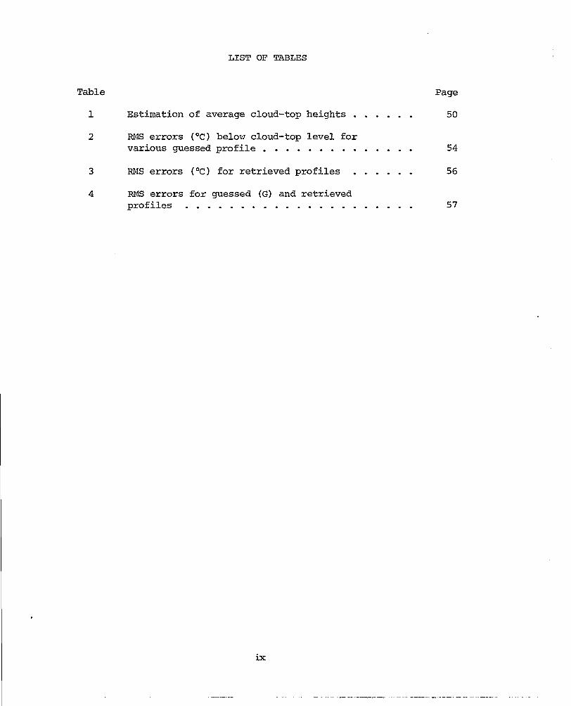
LIST OF TABLES
Table Page
1 Estimation of average cloud-top heights . . . . . . 50
2 RMS errors ("Cl below cloud-top level for various guessed profile . . . . . . . . . . . . . . 54
3 RMS errors ("Cl for retrieved profiles . . . . . . 56
4 RMS errors for guessed (G) and retrieved profiles . . . . . . . . . . . . . . . . . . . . . 57
ix

LIST OF SYMBOLS AND ACRONYMS
a
A
A L
A U
A*
A Total
B
B 1:
co2
C
c
c1'c2
G
H2°
I
E
F* 1*
I MEAS
'CD
I CLR
used to denote the power to which weighting function raised
effective cloud amount (A=Ns)
effective cloud amount for the lower of two layers
effective cloud amount for the upper of two layers
a function of AL and A . U
sum of effective cloud layers
Planck function (radiance)
Planck radiance at frequency r
carbon dioxide
a numerical correction
a computed estimate of C
constants used in computing temperature
the quantitative difference between the average radiances arising from the clear and cloudy portions of a field of view (FOV)
water vapor
clear column radiance
measured radiance for a cloudless atmosphere
measured cloud-contaminated radiance
a computed estimate of ?*
measured radiance
average radiance arising from the cloudy portion of the FOV
average radiance arising from the clear portion of the FOV (equivlanet clear column radiance when obtained by filtering cloud effects)
clear column radiance averaged over many FOVs
X

1. INTRODUCTION
1.1 The ALMA code The ALMA (&xi-symmetrical Lateral Momentum Analyser) computer program is concerned with the numerical computation of two-dimensional coaxial jets with large lateral pressure gradients. The jets may be free or confined, laminar or turbulent, reacting or non-reacting.
In its present version, ALMA predicts the mass fractions of the products of combustion of hydrogen and oxygen, based on the assumption of chemical equilibrium.
1.2 Connections with previous work Under a previous contract (NASl-12167), a computer code, CHARNAL, was developed for predicting the mixing and combustion of turbulent coaxial hydrogen-air jets. CHARNAL was based on the assumption that the pressure of the gases varied with axial distance only; lateral pressure gradients were regarded as negligible. ALMA accounts for these lateral pressure gradients.
The common features between ALMA and CHARNAL are: 0 Both codes account for the effects of temperature and
composition on local fluid properties such as laminar viscosity and specific heat of the gas mixture.
0 Both codes allow for incorporating any inlet-flow conditions (temperature and velocity etc.).
l Both codes have provision for printing some or all of the dependent variables at pre specified axial distances, or after a certain number of marching steps.
1.3 Layout of the report The remainder of this report isdivided into four sections. Section 2 is concerned with the mathematical formulation and physical models employed in ALMA. Section 3 outlines the

SIMPLE algorithm used to link the lateral momentum equation with both the continuity and streamwise momentum equations.
In Section 4, sample predictions for some test cases specified by NASA Langley are discussed. Suggestions for further extensions and refinements of ALMA are included in Section 5. Appendix C details the input quantities required
for using ALMA.
2. THE MATHEMATICAL AND PHYSICAL ANALYSIS - . 2.1 Introduction
This chapter details the mathematical and physical basis of
the ALMA code. Section 2.2 is concerned with the conservation equations of momentum, stagnation enthalpy and chemical species. Section 2.3 describes the turbulence model; and in Section 2.4 the chemical-equilibrium combustion model is discussed.
2.2 The mean-flow conservation equations The differential equations listed in this section are the ones which express the conservation of momentum, mass,
energy and chemical species in a two-dimensional,axi-symmetric, boundary-layer* flow with large gradients of lateral
pressure.
The streamwise momentum equat-ion:
PU au ap la .-& + pv .-?!I! = - - + -
ar ax r x (1J-p $1 (1)
The lateral momentum equation: (viscous terms being neglected)
av ap Pu$+pvar=-ar (2)
* "Boundary-layer", in this context, refers to the characteristic absence of influences from downstream on upstream events.
2

The continuity equation:
& (pu) + + -& (pvr) = 0 (3)
Conservation equation of the mixture fraction (E the ~.- - mass fract!on of hydrogen in any form) (f): -~
af pux+ pvZ$=+&(rfr$
Conservation of stagnation enthalpy (3):
aTi pu ax + pv * = + -& (I?$" -$
+ L-i!- r ar
(ru t (1 -
&)hj 21 (5) h
(4)
The temperature of the mixture, T, is obtained from known values of $,v,u and the mass fractions of the chemical constituents of the mixture as follows:
u2+v2 L 2 -k=h=im.h. 3 3
The species enthalpy,h.,is defined as : J T
I
h j ' / %J
dT+H T JyTref
ref
(6).
(7)

where, T ref is the temperature of the state from which enthalpy is measured, is usually taken as 298.15 K, and H
j'Tref denotes the heat of formation of the species
j at Tref - Equation (2.2-7) can then be written as
T h
j= / 'PA dT + Hj,298.15 K (8) 298.15 K
T =
/ cp j dT + (H.
, J,298.15 K - (h298.15 K - ho ,)I
OK
= %j
T + Ho
T here “p,j , defined as 1
;I; / 'P,J .dT, denotes a mean
OK
specific heat, and Ho is defined by:
HO ' Hj,298.15 K - (h298.15 K - hO K)
(9)
(10)
2.3 The turbulence model
2.3.1The turbulent viscosity The effective turbulent-transport coefficients ut, rh, Tf
are determined by means of the k-E model of turbulence
(ref. 1). According to this model, the magnitude of the viscosity depends only on the local values of the turbulence kinetic energy, k, on the dissipation rate of turbulence
energy, E, and on the fluid density. This turbulent viscosity
l-k' is given by:
I-it = CD p k2/c (11.)
where C is a constant. u
4

The quanC;it..ic:s 1~ antI E at-o c:om~)uI,c?d for oa(:h point in thr?
field by way of the following pair of transport; equations:
(12)
pi ax + pv $5$ = + i& ($i r -25) + Cl i ut (-k)2 a& 2 - c2 y
E (13)
2.3.2 The concentration fluctuations Another important turbulence quantity is the time-mean square of the fluctuations of mixture fraction g. This quantity can be used to account for the effect of turbulence on the rate of chemical reaction (Ref.2) or to estimate the width of a turbulent-flame brush (Iief.3). In ALMA, this width, which is defined as the region of flow over which the stoichiometric conditions occur, is calculated as follows.
First, the magnitude of the mean-square fluctuations of the mixture,fraction, g, is found from the solution of the follow- ing transport equation developed by Spalding (lief.4):
h3 3 pUax+pV$f=F~ l ’ (2 r s)+ Cgl ut
55
(i?&2 - cg2 y
(14)
In the above equation, the values of the constants u C l3' gl
and C @
are 0.7, 2.8 and 2 respectively.
Secondly, a battlement-shaped distribution of the mixture fraction vs time is assumed (Ref.3); this means that the
instantaneous mixture fraction fluctuates rapidly between an upper and lower value, and spends no time in between. From this distribution, and from the values of f and g, the upper and lower values, f, and f-, 0.C the inslantaneous mixture fraction are calculated.
5

Finally, the width of the !.urbulent flame brush at any downstream location is obtained by determining the two. radii at which f, and f equal fst.
2.4 The combustion model 2.4.1Equations
Reference (5) describes an equilibrium-chemistry model, developed and used in conjunction with the CHARNAL computer program to predict the properties in a hydrogen-oxygen flame. The main features of the model are described below.
Four equilibrium reactions are assumed as follows:
o+o + O2 (15)
H+H -+ H2 (16)
H + OH + H20 (17)
0 + II -t OH (18)
The six species involved in these reactions are considered to be present in the mixture, together with nitrogen, which
is inert. To assist in developing the equations to predict
the equilibrium concentration of the sljecies, two intermediate quantities are defined, namely:
wH2
f - mR2 + mH + - 'HZ0 mH20 +!!Lm
woII OH (19)
and wO Frm -I-mo+- wO
O2 'OH mOH + - 'Hz0 mH20 (20)
6

where f is the total mass fraction of hydrogen in any form, and F is the total mass fraction of oxygen in any form.
Also required is the auxiliary relation which states that the sum of the mass fractions of all elemental species must be unity:
f+F+mN =I (21) 2
One assumption is now introduced: it is presumed that the coefficients of turbulent diffusion of the chemical species are equal to each other at every point in the flow. A well-
known consequence is that f is linearly related to mN ; and
the constants in the relation can be determined from 2the
boundary conditions:
(22)
What remains now is to define the necessary equilibrium constants.
As is common in thermodynamics, the equilibrium constant,
K P'
is defined for the reaction aA + bB --> CC by:
K pZ XE pc-a-b
b 'A" 'B
(23)
where p is the pressure in atmospheresand X. is the mole J fraction of species j. For each of the four reactions in the present model, (c-a-b) equals -1.
It is convenient to express the concentrations in terms of mass fractions using the relation:

2.L. mj W j (24)
Substitution of equation (24) into (23) permits derivation ' of the modified equilibrium constant K', thus:
P
K’. = P Kp P W
wE m,C b=
't 'B b
mi mB (25)
The modified equilibrium constants for the reactions (15), (16), (17) and (18) can then be written as:
, mH2 K1= 2
mH
m02 Ka = - 2
mO
K; = mH20
mH mOH
and
K4 = mOH mO mH
(26)
(27)
(28)
(29)
If thermodynamic equilibrium prevails, the K"s take values which depend upon temperature alone. Their values are given
in Appendix B.
In the above set of equations, there are 7 unknowns
Cm H2'
mo2, mop moH’ mH20p mN2 and F; f being given) and
8

7 equations C (19), (20), (21), (2G), (27), (28) and (29)) .
The problem is therefore soluble.
2.4.2 Solution procedure The solution procedure is an iterative one, operating on the two equations:
-II- ii- m02= __ ___- _I- --.- ______ -.I!-.-. -
[
B+hm + 9 I12 ,LEj-J
17 /m,,Z u + P m1r2+ % VT 2+*
2 Iii 2 1
(30)
d- -~ f
mH2= AL ---. ; -__- ____- -_.- --.--_-I
1
z+Ljj -+ --____ -- .-
17 2 "b(
m02 1
ii+&, m JT/-+{ ~
1 + & Cd mo2 f
2 1 i
(31)
---- Here the quantities A.U,C,D are defined by:
1 A= -
r-- K1
1 BY -
r- K2
> c = K; K4
, K; K2 d
(32)
(33)
(34)
and (35)

These quantities depend upon temperature alone, and can be
tabulated at the start.
Equations (30) and (31) have been derived from equations
(19), (20), (21), (26), (27), (28) and (29) by straight- forward algebraic manipulation, including the use of the formula for the roots of a quadratic equation.
Because the RHS of equations (30) and (31) contains mC and
mH as well as f and F, iteration is necessary. Direc 3 su i3 stitution of the latest guesses for m employed in ALMA, H2
and m O2
is and has been found to be satisfactory in
the circumstances which have been investigated; but a Newton-Raphson technique could be employed if divergence were encountered.
3. THE NUMERICAL SOLUTION PROCEDURE 3.1 Introduction
The numerical procedure, employed here to solve the set of partial differential equations that govern the flow and
combustion of axi-symmetric boundary layers, is of the marching-integr-ation type. Because of the need in supersonic flows to solve the lateral momentum equation (2) simultaneously with the other conservation equations, a new
algorithm (SIMPLE E Semi Jmplicit Pressure Linked Equations) is introduced to link the streamwise and radial momentum equations with the continuity equation, so as to obtain a
pressure field. The remainder of this chapter outlines the basic features of this algorithm and of the numerical procedure.
10

3.2 The finite-difference grid Figure 1 shows a portion of the finite-difference grid on
the x-r and the x-w coordinates, where w is a dimensionless
stream function (Ref.6).
The variables u(the x-wise velocity component), p(the pressure), and p(the denisty) are all defined at the grid nodes. The lateral velocity component, v, is defined at locations (o's) midway between those of the u-velocity, as shown in Figure 1, in conformity with usual "staggered-grid" practices. The definition entails that the pressures, of which the differences affect v, straddle the v location.
3.3 The formulation of the solution algorithm Three main steps are followed here to formulate the solution algorithm. The first step is to use the Patankar-Spalding --___- ~- (Ref. 6) procedure to obtain a formula which connects the value of a dependent variable at a downstream node with its value at an upstream node. The second is to use the lateral momentum equation to derive a formula which relates the radial velocity component at a node (i + 4) to the pressures
at the nodes (i + 1 and i) which straddle the v-node at the same axial location. The third step is to derive a"pressure correction" equation and use it to determine a pressure field which satisfies both the streamwise and lateral momentum equations and the continuity equation.
Each of the above three steps is discussed below.
11

3.3.1 The Patankar-Spalding procedure- This procedure is detailed in Reference 6, therefore only the main features are discussed here.
W The primary differential equations (1),(4),(5),(12), (13) and (14) are transformed so that the independent variables are the longitudinal distance x and the
dimensionless stream function w defined as:
w f (Y - y,>/(yE - ‘1) (36)
where Y is obtained from
a\y ar = pur
Subscripts I and E refer respectively to the "inner"
and "outer" boundaries of the flow. The resulting differential equations are all of the form:
2ii ax + (a + bw) -$$ = $j (c -$$ + d (37)
where the terms on the left-hand side represent convection and those on the right hand side express the diffusion and.source of the variable @. The coefficients a and b are functions of the entrainment rates, whilst c involves the effective diffusion
coefficient.
12

(ii) The differential equations are expressed as finite- difference equations, connecting the values of r$ at the nodes i, i + 1, i - 1 (Figure I) at a downstream station D with those at the corresponding nodes at the upstream station U. The general form of the finite- difference equation is:
Di #i D = Ai @i+l D + Bi @i-l D + Ei Q’i,U + Gi $i+l,U , , J
+H iiL +si l-l,u (38)
where A., B., etc., 1 1
are treated as constants, the expressions for which are deduced by integration of the differential equation (37) over a control volume surrounding the node where $i prevails.
(iii) The integration proceeds by "marching" downstream, the values of tii at station D being calculated from those at station U.
At each forward step, new values are ascribed to YE
and YI, the stream functions at the grid boundaries. These values, together with the continuity equation, determine the geometrical locations of the boundaries.
3.3.2 The relation between v and p The relation between v and p is obtained by integrating the lateral momentum equation (2). The finite-difference form
of this relation is:
(39)
where the notations of Figure 1 are used.
13

Equation (39) shows that a solution for v. 1+4 ,D
cannot be obtained in an explicit manner since the radial pressure
distribution at D is not a pre-specified quantity. This problem is dealt with in the following section.
3.3.3 The pressure correction procedure (SIMPLE) The central idea of the pressure-correction procedure is to make an informed guess of the pressure distribution at the downstream station D; then corrections are added to the pressures, and to the velocity components u, v, to ensure compatibility of flow areas.
In this section it is aimed to derive a pressure-correction equation of the form:
-'i+$ Pf+l - Ci-& pi-1 + c
AT 'i+$ + c i-4
= AI - a; (40)
where the superscripts (*) and (') denote respectively a guessed quantity and,a correction component. In equation
(40) the right-hand side is the area-discrepancy appropriate to the guessed velocity field; A* being the flow area associated with,the continuity and streamwise momentum
* equations and a being the area associated with the lateral momentum equation. The c's are coefficients having the dimensions of area divided by pressure.
It is important to note that the solution of the pressure- correction equation (40) yields a pressure-correction component which, when added to the guessed pressure, cancels the discrepancy in the flow areas.
Equation (40) will now be derived.
14

Three steps are followed in the derivation. The first is to obtain a pia' relation; the second is to find a p'%A' relation, and the third is to combine those two relations to produce equation (40).
p;Ca' relation It is sought to obtain an equation in the form:
a: = c 1 i+$ (Pf - Pf+l) + ci-$ (Pf - pi-1) (41)
where c's are coefficients having the dimensions of area divided by pressure. The starting equation is that which links v and p, i.e. equation (39).
Let the downstream quantities u,v,p,p,A,a,r be composed of two components according to:
P = P* + P' u = u* + u0
v = v* + v/
P = P* + P’
A = A* + A' a = a* + a' r = r* + r0
(42)
(43)
(44)
(45)
(46)
(47)
(48)
Substitution into equation (39) of the values of p,u,v,p,r from equations (42), (43), (44), (45) and (48), followed by subtraction of the resulting equation from (39) yields:
Vf+$ = P > p*u* i+B (49)
where P, u and r are approximated by their guessed values.
15

Another equation is required to connect a! with v'; this
is obtained by referring to Figure 1. The cross-stream area a i,at D, for the shaded control volume associated with
node i can be calculated from:
a. = a 1 i,U
+ Jr 1 i+i,U tan a i+$ - 'i-$,U tan aiBl 6x I
2 1
(50)
where a i u is the upstream cross-stream area. The inclination a of the constant-w lines is given by:
- II V a= --k U (51)
* II where m is the rate of mass flow across the constant-w line.
Substitutioninto equation (50) of the values of a,r,v,u,v'
from equations (51),(48),(44),(43) and (49), followed by subtraction of the resulting equation from equation (50), leads to the desired equation (41), where c now has the value r 62x/(6r p* u*2).
p'%A'relation The desired p'%A'equation is
Af =- < - 1 * *2
>
A; p; YPi Pi ui
(52)
which expresses the effect of pressure change on the down- stream cross-stream area. Three equations are employed to
derive equation (52). These are the continuity, the
streamwise momentum equations and the gas-law relation for isentropic expansion.
The mass flow rate across the downstream face of the shaded control volume (Figure 1) is:
16
I

Pi Ui Ai = (YE - ‘I>(Wi+l - Wi-l)
= a; u; A; (53)
Substitution into equation (53) of the values of p,u,A from equations (45), (43), (46) gives:
p; Uf A; * +*+* = 0 Pi Ui Ai
(54)
where the terms containing the cross products p'u< p'A; u'A; p'u'A' have been neglected.
Now the variation of u with pressure can be estimated by noting that, if the shear stresses and body forces are supposed to be uninfluenced by the pressure change, the streamwise momentum equation (1) leads to:
du 1 dp = - pu (55)
The substitution of equations (42), (43), (45) into (55) yields:
u: = - 1 . 1 * * pi
Pi ui (56)
Further if the process of pressure adjustment is assumed to be isentropic, then:
* 'i pf = - YP*i
Pi (57)
Now the p/s A'equation (52) can be easily deduced by combining equations (54), (56) and (57).
17

Finally the pressure-correction equation (40) can now be
obtained by noting that the net effect of the pressure-
correction process is to cancel the discrepancy in the calculated cross-stream flow areas, i.e. Ai should be equal
to ai or
(58)
The direct substitution of equations (41), (52) into (58)
produces the pressure-correction equation (40) for the node
i; similar equations are obtained for all the nodes across
the grid.
3.4 Conditions at the E-boundary in supersonic flow ---_I.-L When the free stream is supersonic, the values of u and v
at the E-boundary are evaluated from the following two
equations:
[u2 - UllE = (P, - P1)/(P1 ul) (59)
and p2 - y1]F = 't;Yl tanbl+sin-lh-)J - tan aI} (60)
i 11
where the notations of Figure 2 are used, and cl is the speed of solAnd at station 1.
18

Equation (59) is derived from the one-dimensional streamwise momentum equation for the shaded control volume (Figure 2). Equation (60) is obtained by combining the equations of continuity and lateral momentum for the shaded control volume and then substituting for the angle (0 --c1 l) between the streamline and the shock from small-wave theory. t
It is seen from equation (60) that the velocity.v2 at the E-boundary can be calculated in terms of quantities immediately upstream. The pressure p2 at the E-boundary is set equal to the value calculated at the near-boundary node.
3.5 The basic solution steps The solution procedure will now be reviewed, based on a consideration of the portion of the finite-difference grid shown in Figure 1. The variables at station D are to be determined by the integration of the governing differential equations over the shaded control volume. This integration is performed as follows:
a> The pressure gradient across the forward step is guessed; the pressure p* at station D is then calculated.
b) Equation (1) is integrated as in Ref. (6). The resulting velocities at D are only estimates since they result from a guessed pressure field.
-~- -- ~--. -------i-~.- ___~.
t From small-wave theory, the angle (0 --o! l) is given byi
e- a1 = sin-1 r&1 where c l is the speed of sound at station 1.
19
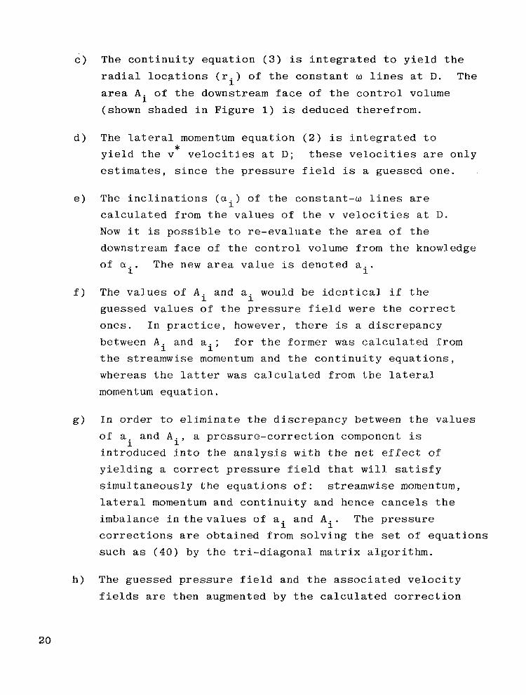
c>
d)
e>
f>
g>
h)
The continuity equation (3) is integrated to yield the
radial locations (ri) of the constant w lines at D. The
area A. of the downstream face of the control volume
(shownishaded in Figure 1) is deduced therefrom.
The lateral momentum equation (2) is integrated to yield the v* velocities at D; these velocities are only estimates, since the pressure field is a guessed one.
The inclinations (ai) of the constant-w lines are calculated from the values of the v velocities at D. Now it is possible to re-evaluate the area of the downstream face of the control volume from the knowledge of c1..
1 The new area value is denoted ai.
The values of Ai and ai would be identical if the guessed values of the pressure field were the correct ones. In practice, however, there is a discrepancy between Ai and ai; for the former was calculated from the streamwise momentum and the continuity equations, whereas the latter was calculated from the lateral
momentum equation.
In order to eliminate the discrepancy between the values of a. and Ai, a pressure-correction component is intrtduced into the analysis with the net effect of yielding a correct pressure field that will satisfy simultaneously the equations of: streamwise momentum, lateral momentum and continuity and hence cancels the imbalance inthevalues of a i and Ai. The pressure corrections are obtained from solving the set of equations such as (40) by the tri-diagonal matrix algorithm.
The guessed pressure field and the associated velocity fields are then augmented by the calculated correction
20

components; the result is a more correct flow field,
which certainly satisfies continuity, and which satisfies momentum as accurately as is desired .
i> The above operations (a to h) complete one integration step; they are to be repeated for successive forward steps until the whole domain of integration has been covered.
4. DISCUSSION OF SAMPLE PREDICTIONS To demonstrate the general capabilities of ALMA, five test cases have been computed; these involve the mixing and combustion of two coaxial jets of hydrogen and air. The geometry and the initial conditions for the test cases are given in Figure 3 and Table 1.
In this section, the results are presented in the form of radial profiles of the quantities u,v,T,k,c,f,g,R and of the mass fractions of the species 02, H2, H20, H, 0, OH and N2 in Figures 4 to 17 inclusive. Because the values of the above quantities vary by orders of magnitude and are plotted, at a given station, for convenience in two figures, each is normalized by reference to its maximum and minimum values in the profile, so that the normalized values extend from 0 to 1.
4-l -- The jet surrounding a centre-body Case 1. The results are discussed by examining the radial distributions ofthequantities u,v,T,k,e,f,g and R and the mass fractions of species at three different downstream stations: x/Y.
J = 20, 60 and 100 (Figures 4,6,8,5,7 and 9).
Profiles at x/Yj = 20
Figure 4 shows that at x/Y. = 20 (i.e. J
nearest to the nozzle) all the predicted quantities behave as expected. For example, the u-profile exhibits a steep gradient near the
21

Table 1. Initial Conditions of the Test Cases
Test Test Case Case 1 1 2 2 3 3 4 4 5 5
pI c105N/mg 1. 1. 1. 1. 1. 1. 2. 2. 1. 1.
pE; (105N/m2) 1. 1. 1. 1. 1. 1. 1. 1. 1. 1.
TI TI ( K) ( K) 316. 316. 180. 180. 247. 247. 247. 247. 247. 247.
TE TE ( K) ( K) 885. 885. 885. 885. 1459. 1459. 1459. 1459. 1459. 1459.
TW TW ( K) ( K) 300. 300. 300. 300. 900. 900.
UI UI (m/s> (m/s> 1303. 1303. 2100. 2100. 2389. 2389. 2389. 2389. 2389. 2389.
uE uE crnb> crnb> 1800. 1800. 1800. 1800. 1432. 1432. 1432. 1432. 1432. 1432.
Y Y j j (m) (m) 3.00264 3.00264 0.00264 0.00264
R R j j b-0 b-0 0.00238 0.00238 0.00238 0.00238 I.00238 I.00238
Rw Rw Cm> Cm> 3 . 01214 3 . 01214 0.01214 0.01214 3 . 01633 3 . 01633
mo2 mo2 ; outer .232 ; outer .232 .232 .232 . 232 . 232 .232 .232 .232 .232
FN FN ) ) jet .768 jet .768 .768 .768 . 768 . 768 .768 .768 .768 .768 2 2 > >
mH mH ) ) inner 1. inner 1. 1. 1. 1. 1. 1. 1. 1. 1. 2 2 > > jet jet
22

centre-body wall and a lesssteep one in the shear layer between the jet and the free stream.
Also, as is well known, the k-profile (Figure 4) attains a maximum at about the middle of the shear layer where both u and v have large gradients. The dissipation rate of turbulence energy is highest near the wall, where the length scale of turbulence is at its minimum.
Chemical reaction is evident by the peak in the temperature profile (Figure 4) at the radial location where the mixture fraction, f, attains its stochiometric value, f St' of about 0.028.
The mean square of f-fluctuations, g, reaches its maximum value where f has its steepest radial gradient; this is as expected.
Figure 5 shows that the radicles 0 and OH have their maximum concentrations at the peak temperature, whereas H attains its highest value at a slightly lower temperature towards the hydrogen-rich region.
It is also displayed in Figure 5 that the profiles of H2 and O2 overlap in a small region centered around the location of f St' The two species N2 and H20 exist in considerable concentration over the whole domain, thought their peaks lie in the air-rich and the hydrogen-rich regions respectively.
Profiles at x/Y. = 60
Figure 6 shows that at a distance 60 Y. downstream, the shear J
flow develops and the initial step-shaped u-profile becomes relativelysmooth. The maximum values of k and E are consequently lower than those at the upstream station of 20 Y..
J
23

The temperature profile still has its maximum near the
location of fst. The value of this. maximum is 30% higher
than that at the station of 20 Y.; this is due to the J
development of chemical-reaction as indicated by the lower
value of m H2
(Figure 7).
Profiles at x/Y. = 100 J
Figure 8 shows that at a distance of 100 Y., the u-profile 3
is similar to that at 60 Y.. Also, R are similar to those at ;O Y.,
the profiles of k and though the level of k is
slightly lower and the maximumJE is higher than that at 60
Figure 9 displays the profiles of the species concentrations at x/Y. = 100.
J Here the maximum value of mH , near the wall
+ .of the centre-body, is only 15.8% of its in1 la1 value at the nozzle exit.
Comparison between Cases 1 and 2. Now the predictions of
case 2 at 100 Yj (Figures 10 and 11) are compared with those of case 1 at the same station. Both cases have the same geometry and initial conditions, except that in case 2 the
initial u-velocity of the hydrogen jet is 50% larger than that in case 1.
Figure 10 shows that the u-profile is not yet fully developed; it still retains the step shape of the initial distribution.
This behaviour is explained in what follows. Here, the temperature level is lower than in case 1, because the shear layer is predominatly richer in fuel than in case 1; the maximum values of f and m
H2 are 0.31 and 0.286 as compared
to their respective values of 0.182 and 0.158 in case 1. Lower temperatures result in higher densities and hence a lower rate of velocity-decay.
24

4.2 The jet without a centre-body _-ii Case 3. Figures 12 and 14 show the radial profiles of u,T, k,f,g and R at two downstream-stations: x/D. = 10 and 50.
J The corresponding profiles of the species mass-fractions are shown in Figures 13 and 15.
At a distance of 10 D j .downstream (Figure 12), k reaches its maximum in the high-shear region away from the axis, whereas at a distance of 50 Dj (Figure 14) where the shear flow is developed, k attains its peak at the axis. This behaviour is generally a feature of axi-symmetric jets and is different from that of the jet in cases 1 and 2 because of the presence of the centre-body. .
The temperature profiles at both axial locations have their highest value where f equals fst; this is also where the radicles 0 and OH reach their maximum concentrations (Figures 13 and 15).
Comparison between Cases 3 and 4. The profiles of u,T,k,f, g and R at a downstream distance of x/Dj = 50 for case 4, are shown in Figure 16.
The profiles of the species mass-fractions at the same distance are shown in Figure 17.
The initial conditions of case 4 differ from those of case 3 only in that the static pressure of the hydrogren jet of the former is twice that of the latter. The effect of this higher pressure is seen by comparing Figures 14 and 16. It is evident that both u and f have a lower rate of decay in case 4 than in case 3; this can be attributed to the higher
mass flow rate in case 4 caused by the higher pressure and density. Also the maximum mass fraction of H2 at a distance of 50 D.
J in case 4 (Figure 17) is higher than that of case 3.
25

The confined jet, Case 5.
Regarding case 5, the confined-flow case, it was planned to
continue the integration to a downstream position of 50 D.: J
however, it was not possible to proceed with the computation farther than 10 D.,
J because choking was predicted there.
This choking is detected by the computer program when the calculated flow-area necessary to satisfy the conservation of lateral momentum exceeds that required for conservation of mass (here this is equal to the area of the confining
duct). This situation indicates that the intitial,f.low conditions for case 5 are not compatible with the flow
through the duct. .
It is suggested that new initial conditions should be
specified for this case, e.g. by successively lowering the velocity of the hydrogen jet, and performing further
runs.
26

w
L X
r
I--- X
U D
i
Figure 1: The finite-difference grid in both the x-w and the x-r coordinates.
25 Shock
I f X tan ~1~
X tan 0
Figure 2: Definition of Notat --- - ;ions
27

a - Cases 1 and 2
O2 PE TE
'F N2 32 >
c. L,.
b - Cases 3 and 4
C.L.
c - Case 5
Figure 3 : The Flow Geometry of the Five Test Cases
28

0.6
0.4
0.2
0
0 0. 2 0.4 cl . Cl 0. 8 1 r/YE
Fig.4 Radial profiles of u,T,k,E,f,g,t and v at x)"Y.=20; Case 1. 3
@ @ max @ min @ @ max @ min
U 1804 0. f 0.509 0.
T 1889 300 g 0.07 0.
k 2.4x10 4 0. R 0.016 0. 8
E: 4.8x10 0. V 0. -11.9
29

.
0.6,
0. 4.
0. 2.
0.
--- - -- II 2 (
\ \
=+ -.-\
0. 0.2 0.4 0.6 0.8 1 . r/Y E Fig. 5. Radial profiles of the species mass-fractions at
x/Y = j
20, Case 1.
a 0 max a min Q 0 max 0 min
H 0.495 0. H 1.7ox1o-5 0. 2 -5
O2 0.232 0. 0 7.74x10 0. -4 OH 7.28x10 0. N2 0.768 0.37
H2° 0.234 0.
30

8 8
0.8
0.6
-p--r ----- ------ ----
i \ \ \ . \ i- i \ \ \ \ i \ ‘L, \ \
Fig.6 Radial profiles of u,T,k,f,g and R at x/Yj= 60, Case 1.
@ Qmax @ mln Q, @ max @min
U 1801 0. f 0.265 0.
T 2523 300 g 0.0175 0.
k 1.46x10 4 0. R 0.0187 0.
31

0.6
0.4
0.2
0. I / I
/ I
II /
0. 0.2 0.
Fig.7 Radial profiles of
60, Case 1.
cp @ max @ min
H2 0.244 0.
O2 0.232 0.
OH 3.75x10⁻³ 0.
H2° 0.245 0.
4
the
0.6 0.8 1. r/YE species mass -fractions at x/y.=
7
@ max Cp mfn
4.48x10 -4 0 .
0 1.71x10 -4 0 .
N 2
0.768 0.565
32

0.6
0.4
0.2
0.
--- T ----- f -_---- k -_-o- II
--__--A V
0. 0.2 0.4 0.6 0.8 1. r/Y E Fig.8 Radial profiles of u,T,k,f,R,v at x/Yj=lOO, Case 1.
a @ max @ min (3 0 max @ min
U 1800 0. f 0.182 0.
T 2592 300 R 0.021 0.
k. 1.2x10 4 0. V 0.224 -0.79
33

1.
,z
I
8
0-f
0.6
0.4
0.2
0.
Fig
= 1
(3
H 2
O2 OH
*2O
H 2
---0 2
-----OH --- - --
H2° ---_ H -e--p 0 ------
N2
. 9 Radial profiles of the species mass-fraction at x/Y
00, Case 1.
Q, max @ min aJ Cp max
0.158 0. H 4.41x10⁻⁴
0.232 0. 0 -0016
0.011 0. N2 0.768
0.245 0.
r/Y E
j
Q min
0.
0.
0.628
34

e e
0.8
0.6
0.
Fig. 10. Case 2.
4
u
T
k
E
-. .
\\
\ \
l . .
\
\
L-. u
--- T
\
----- f ------ k ___--- e ----- 4 --es-- f. --_-_-- V
0.2 0.4 0 . 6 0.8 Radial profiles of u,T,k,c,f,g,!L,v at x)'Y
j
0 max @ min @ 0 max
1832 0. f 0.31
2454 300 g 0.021
1.6x10 4 0. !L 0.021
1.3x10 8
0. V 3.35
0 min
0.
0.
0.
0.
35

I / i
/ , ,
/
/ II
! 2
--- O2
---- -011 I -_-- --
/
II 2(
ti -__ -
I ---- -0
0.6 -- I -_---- I
N2
0. 0.2 0.4 0.6 0.8 1. r/Y E Fig.11 Radial profiles of the species mass-fractions
@ @ max 0 min 0 0 max Qmin -4
H 2
0.286 .O. H 3.6x10 0.
O2 0.232 0. 0 0.001 0.
OH 0.0077 0. N2 0.768 0.533
H2° 0.245 0.
36

I I, * I
e <
0.8
0.6
0.4
0.2
0.
\ -p-T
\
-----f
--- - -- k ---.-- R ---p-g
\
\
. I
0. 0.2 0.4 0.6 0.8 1. r/Y E
Fig.12 Radial profiles of u,T,k,f,g and 2 at x/Dj=lO,Case 3.
Q max @ min 0 CJ max @ min
2089 1427 f 0.605 0.
2520 470 g 0.05 0.
4.55x10 4 5.41x10 3 R 0.0052 0.0036
37

0.6
0.4
0.2
0.
1 ./ ! I / I : I 1 -1 I ,A .-Al I I ~- 0. 0!2 0'. --g-h - 4
\
1. r/Yv - Fig. 13 Radial profiles of the species mass-fractions at
x/D. = 10, Case 3. 7
@ @ max @ min a Omax @min -5 H 0.594 0. H 7.4x10 0.
2 0 0.232 0. 0 0.0026 0.
2 OH 0.011 0. N 0.768 0.303
2 H2° 0.234 0.
38

0.6
0.4
0.2
0.
--
\
--- T ----- f ------ k
----- Q
-----
\ g .
\ *.
\
I A I : I \
Fig.14 Radial profiles of u,T,k,f,g and J? at x/D. = 50, Case 7
@ @ max Q, min @ @ max Q min
U 1650 1431 f 0.176 0.
T 2464 1424 g 0.0058 0.
k 1.14x10 4
1.86x10 3
R 0.0092 0.0076
3.
39

I IR E
e 8
0.8
0.6
0.4
0.2
0.
Fig.15 Radial profiles of the species mass fractions at = 50
cp Q max @ min cp @ max
H2 0.1525 0. H 9.5x10 -4
-3 O2
0.232 0. 0 3.55x10
OH 0.017 0. N2 0.768
H2° 0.242 0.
r/Y E x/D.
3
Qmin
0.
0.
0.632
40

0 63
0.8
0.6
0.4
0.2
0. r/Y
E
Fig.16 Radial profiles of u,T,k,f,g and % at x/D. = 50, Case 4.
@ fD max 0 min a Q mZx @min
u 1761 1430 f 0.21 0.
T 2734 1210 g 0.0076 0.
k 2.16x10 4 1.85x10 3 R 0.01 0.008
41

I
0 .
0.8
0.6
0.4
0.2
0. .
Fig.17 Radial profiles of the species mass-fractions at x/D.=50, Case 4.
3 a @ @ (3 a -4 H 0.191 0. H 8.72x10
2 3.7x10
-3 0 0.232 0. 0
2 OH 0.018 0. N
2 0.768
r/U E
QI
0.
0.
0.604
H2° 0.241 0.
42

5. ----- SUGGESTIONS FOR FURTHER EXTENSIONS AND REFINEMENTS OF ALMA -- The following extensions and refinements to ALMA are easily possible; and they may prove to be necessary when the predictionsof ALMA are compared with experimental data:-
(a) In*roduct-ion of-realistic chemistry As has been explained, thermodynamic equilibrium has been postulated in ALMA; the chemical reaction rates have been presumed to be very fast. The presumption is at best an approximation to the truth; and it will undoubtedly be necessary, from time to time, to examine how the predictions will change if chemical- kinetic limitations are allowed for.
These limitations may be of two kinds: those associated with the chemical kinetics of laminar-flow processes; or those concerned with "eddy break up". New ideas (Ref.2) concerning the interactions of these two modes are now available; and the ALMA code can be easily extended to accommodate these ideas.
The extension naturally takes the form of the provision and solution of further differential equations, together with auxiliary relations concerning sources. However, in order that the associated computer time does not become excessive, simultaneous improvements in the numerical procedures discovered since ALMA was conceived, may be advantageously introduced.
(b) Introduction of "partially-parabolic" effects --- ALMA is an advance over CHARNAL, in that it takes account of the lateral-momentum effects in the supersonic-flow regions. However, wheretheflow is subsonic, the variation of pressure with radius has to be ignored if the marching nature of the integration is to be preserved.
43

In some ci3*cumsta.nces, the inaccuracies resulting
from this practice are not to be tolerated.
Fortunately, experience now exists of handling the lateral-momentum effects in subsonic regions by the so-called "partially-parabolic" method (Ref.7 ).
It is true that repeated marching integrations must be made, to this end; so computer time increases. However, the partially-parabolic method is economical of storage: only the pressure has to be stored for the whole two-dimensional flow field; so the storage requirement is scarcely greater than that of ALMA.
(c) Allowance for small patches of recirculation.
In a still further extension, "elliptic" flow regions may be incorporated. These require still further storage. However, recent coding developments (Ref. 8')
,have permitted the additional storage, and the more
numerous iterations, to be restricted to the regions of recirculation themselves. It is not necessary, just because shock-wave-boundary-layer separation occurs in one area, to forego entirely the economies associated with marching integration.
This refinement will also be important if it should become important to compute the influence of the finite thickness of the "lip" of the hydrogen-injection nozzle.
Of course, the stream-line coordinate system must be abandoned, at least in the recirculation region. However, means exist of retaining its advantages
elsewhere.
44

APPENDIX A. Symbols
A
a
C
c1
%,j D.
J F
f
f st
g
h
H j'Tref
ii
K P
Ki K;
k
R
m. J
cross-sectional flow area of a control volume in the continuity equation;
cross-sectional flow area of a control volume in the lateral momentum equation;
coefficients in the pressure correction equation;
constants coefficients appearing in turbulence model;
speed of sound;
mean specific heat of species j;
diameter of jet nozzle;
mixture fraction of elemental oxygen;
mixture fraction or mass fraction of elemental hydrogen;
stoichiometric value of f;
mean square fluctuations of f (- f'2):
enthalpy;
heat of formation of species j at T = Tref
stagnation enthalpy;
general equilibrium constant;
equilibrium constant for the reaction i;
modified equilibrium constant;
kinetic energy of turbulence;
length scale of turbulence = k 3'2/E;
mass fraction of species j
45
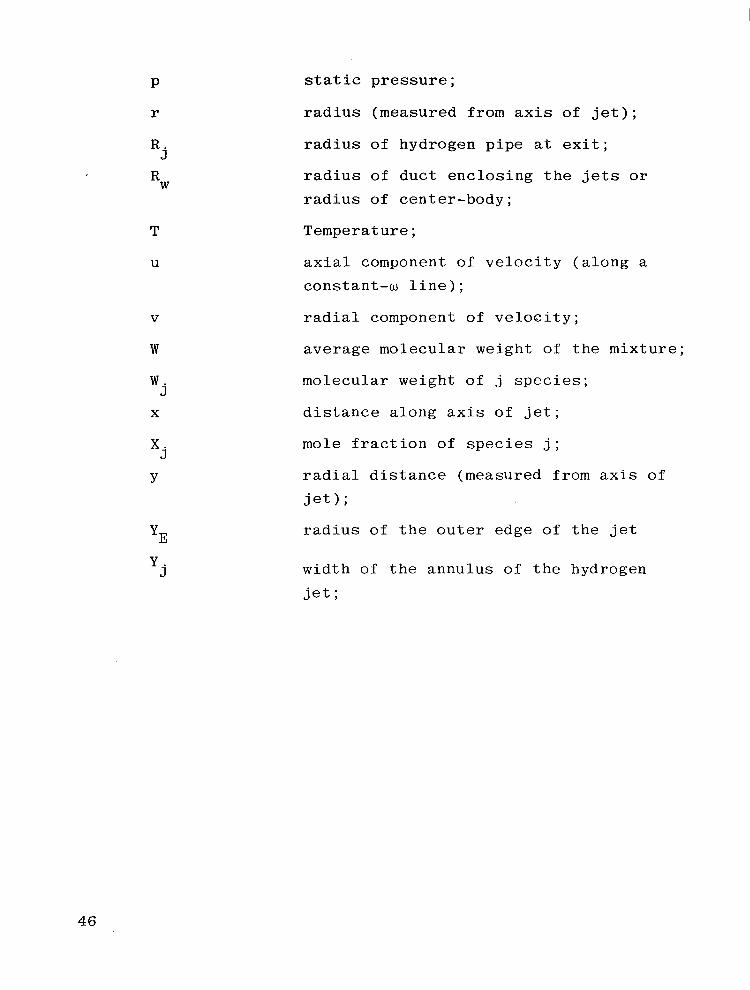
P
r
R. J
RW
T
U
V
w
W. J
X
X. J
Y
yE Y.
J
static pressure;
radius (measured from axis of jet);
radius of hydrogen pipe at exit;
radius of duct enclosing the jets or radius of center-body;
Temperature;
axial component of velocity (along a constant-w line);
radial component of velocity;
average molecular weight of the mixture;
molecular weight of j species;
distance along axis of jet;
mole fraction of species j;
radial distance (measured from axis of
jet>;
radius of the outer edge of the jet
width of the annulus of the hydrogen
jet;
46

Greek Symbols Symbol --
a
Y
8
angle between the constant-w line and axis of jet;
the ratio of specific heats;
angle between a streamline and axis o.f jet;
rate of turbulence energy dissipation;
density;
general variable;
stream function;
non-dimensional stream function;
Superscripts
Symbol
* estimated quantity;
correction component except in the definitions of the chemical equilibrium constants.
‘47

APPENDIX B. Table of Equilibrium COnStantS
Temp. Kj
200 5.0+100 3.1E+99 2.6tlOO 2.6+100 4.4E-51 1.7E-50
400 2.8Bt52 2.7E+58 3.2Et51 6.2Et59 5.9E-27 6.OE-30
600 2.3E+33 4.3~+36 5.8E+32 .9.OEt37 ~.OE-17 4.7E-19
800 5.9Et23 4.9E+25 2.2Et23 9.3E+26 1.28-12 1.4E-13
1000 9.7E+17 1.2E+19 4.5E+17 2.2Et20 l.OE-09 2.7E-10
1200 1.2Et14 5.OE+14 7.OEt13 8.2Et15 8.7E-08 4.4E-08
1400 2.1E+ll 3.5E+ll 1.2E+ll 5.4Et12 2.1E-06 1.6E-06
1600 1.7E+O9 l.lE+09 l.lE+O9 2.2E+lO 2.4E-05 2.5E-05
1800 3.9E+O7 2.1E+O7 2.7E+07 3,OE+08 1.5E-04 2.1E-04
2000 1.9.E+06 7.03+05 1.4E+06 9.8EtO6 7.2E-04 l.lE-03
2200 1.5E+05 4.3Et04 1.2Et05 5.8EtO5 2.5E-03 4.8E-03
2400 1.9Ei04 4,2E+03 1.6Et04 5.5Et04 7.OE-03 1.5E-02
2600 3.4E+03 5.8E+O2 2,8E+O3 7.6Et03 1.7E-02 4.1E-02
2800 7.5E+02 l.OEtO2 6.4E+O2 1.3E+03 3.6E-02 9.6E-02
3000 2.OEt02 2.4E+Ol 1.74+02 3.1E+02 7.OE-02 2.OE-01
3200 6.3EtOl 6.8E+OO 5.7E+Ol 8.5E+Ol 1.2E-01 3.8E-01
3400 2.3E+Ol 2.1E+O0 2.1E+Ol 2.7E+Ol 2.OE-01 6.7E-01
3600 9.3E+Ol 7.9E-01 8.6EtOO 9.8EtOO 3.2E-01 l.lE+OO
3800 4.1EtOO 3.2E-01 3.8EtOO 3.9E+OO 4.9E-01 1.7E+OO
4000 1.9EtOO 1.4E-01 1.8E+oo 1.7EtOO 7.OE-01 2.6EtOO
4200 l.OE+OO 6.8E-02 9.8E-01 8.3E-01 9.8E-01 3.8E+OO
4400 5.5E-01 3.5E-02 5.4E-01 4.2E-01 1.3EtOO 5.3E+OO
4600 3.2E-01 1.8E-02 3.1E-01 2.2E-01 1.7EtOO 7.2E+OO
4800 1.9E-01 l.OE-02 1.9E-01 1.3E-01 2.2E+OO 9.6E+OO
5000 1,2E-01 6.4E-03 1.2E-01 7.7E-02 2.8E+OO 1,2E+Ol
5200 7.9E-02 4,OE-03 7.8E-02 4.8E-02 3,5E+01 1.5E+Ol
5400 5.3E-02 2,5E-03 5.3E-02 3.]E-02 4,3EtOO 1.9E+Ol
5600 3.6E-02 1.7E-03 3.6E-02 2,0E-02 5.2EtOO 2.4E+Ol
5800 2.6E-02 l.lE-03 2,6E-02 1.4E-02 6.1EtOO 2.9E+Ol
6000 1.8E-02 8.1E-04 1.8E-02 9.8E-03 7.2E+OO 3.5E+Ol
K; K; ii ii c’
2.42Et50
4.3Et29
1.09Et19
4.35E+13
2.94E+lO
2.14E+O8
5.22E+O6
3.67Et05
4.53Et04
8.63E+O3
2.24E+d3
0.71E+03
2.6E+02
1.11E+O2
5.37EtOl
2.95EtOl
1.70E+Ol
1.02EtOl
6.38EtOO
4.30E+OO
3.12EtOO
2.2OEtOO
1.59EtOO
1.30E+OO
9.62E-01
7.49E-01
6.20E-01
4.85E-01
4.22E-01
3.44E-01
ij
1.95EtOO
2.19Et04
8.46EtO2
1.56Et02
5.94EtOl
3.14E+Ol
1.81E+ol
1.32EtOl
9.45EtOO
7.76EtOO
6,96E+OO
5.77EtOO
5.30EtOO
4.49E+OO
4.37E+OO
3.87E+OO
3.62E+OO
3.45E+OO
3.25EtOO
3.09Et00
3.09EtOO
2.89E+OO
2.69E+OO
2.79E+OO
2.59E+OO
2.52E+OO
2.53EtOO
2.49E+OO
2.47E+OO
2.47E+OO
48

APPENDIX C. Input Quantities Required for ALMA
ALMA solves 7 simultaneous partial differential equations for the dependent variables u,v,%,k,~,f and g and employs typically 21 nodes in the radial direction. The program is written in basic FORTRAN IV language and is ready to run on the CDC 6600-series computers (although only minor modifications are required to adapt it to the UNIVAC 11061 IllOor IBM 360 machines). ALMA requires approximately 5 seconds compilation time on a CDC 6600 (FTN compiler) and about 40000 decimal storage locations.
Castellated profiles are assumed for the variation of the dependent variables between the grid nodes and a typical forward step size of 0.2 times the local shear layer width is employed. Approximately 5 axial steps can be executed per second.
The remainder of this appendix is concerned with the information that the user has to provide via data cards and data statements in subroutines MAIN and THERM.
Subroutine MAIN. - --
(i) Control indices in chapters 0 and 1: -- .~
Fortran symbol Significance
ITDIM: Max. number of nodes in the radial direction included in the profile plot (>N+l).
49

UI: .
TI: Temperature of the inner fluid ( K)
PI: Pressure of the inner fluid (N/m2)
02E: Mass fraction of oxygen in the
outer fluid
H20E:
AN2E:
Axial velocity of the inner fluid
(m/s >
Mass fraction of water-vapor in the
outer fluid
Mass fraction of nitrogen in the outer fluid
Wall temperature ( K) TWALL:
Subroutine THERM.
Control indices in entry BEGIN
NR: Number of reactions
NS:
HO:
Npber of species
The quantity {Hj 2g8 I5 K- ,
(h298.15 KBho K)) in equ.(2.2-9)
WM: Molecular weight of each species
considered in the reaction.
50

JTDIM:
ILDIM:
JLDIM:
KASE:
NDATA:
NSTAT:
NPROF:
DXPROF:
NPLOT:
DXPLOT:
LASTEP:
ISTABL:
Max. number of profiles plotted at any axial location.
Max. number of stations included in the longitudinal plots (aLASTEP)
Max. number of longitudinal plots.
Test case number.
Controls whether the input data of the equilibrium constants and enthalpy will be printed (NDATA =. 1) or not (NDATA 3 1)
Number of steps between output stations.
Number of steps between profile stations
Axial distance between profile stations
Number of steps between plot stations
Axial distance between plot stations
Number of steps at which calculation terminates.
Adjusts, if set equal to 2, the forward step DX according to local math number.
51-
.- _ --- ____ -.- -. ..~ - ~. ~---- --___--. - --

, . *.-. . . . . -.,
‘. - _.____. -.-_--.-_L__._- ,-.‘- ::-.‘-..- .._- .- .- ~.--_
. . . .
NRKACT: Controls whether the flow is chemically reacting (NREACl+2) or non reacting (NREACT=l)
MODEL: Equals 2 for turbulent flow and equals 1 for laminar flow.
(ii) Control indices and input data in chapter 2.
N: Number of grid intervals in the radial direction (Ng20)
FRA: Specifies forward step length as a fraction of the width of the shear layer.
KRAD: Specified whether the flow is axi-symmetric (KRAD=2) or plane (KRAD=l).
52
YOUT:
XULAST: Maximum streamwise distance (metres).
KIN: Specifies inner boundary condition. KIN = 1; wall boundary KIN = 2; free boundary KIN = 3; symmetry boundary
KEX:
Width of jet-annulus or diameter or jet-nozzle (metres)
Specifies outer boundary condition KEX = 1; wall boundary KEx= 2; free boundary KEX = 3; symmetry boundary
---__-__-*_. _ --... ‘--F--- ---1_ -‘~ --__------- --..
.- _ .

KONFIN:
CSALFA:
Specifies flow confinement KONFIN = 1; confined flow KONFIN = 2; free flow
Cosine of angle of inclination of streamlines to axis of symmetry
DXLIM: Controls forward step size so that entrainment per step is limited to DXLIM (fluid within boundary layer).
ULIMI: Maximum permissible dimensionless velocity difference at inner free boundary (KIN = 2).
ULIME: Maximum permissible dimensionless velocity difference at outer free boundary (KEX = 2).
(iii)Control indices in Chapter 3.
NF: Specifies the number of dependent variables to be solved for
(iv) Initial conditions in Chapter 5.
UE: Axial velocity of the outer fluid
(m/s >
TE: Temperature of the outer fluid
( K)
PE: Pressure of the outer fluid (N/m2)
53

__ -. . . _ -_ ._ _ -IL-.----. *:-L.--L. .^_. -- - .- .i
Data Cards.
There are 120 data cards to be read in from subroutines THERM and OUTPUT.
The first 99 cards include the values of the chemical equilibrium constants RC(60,NR) of the NR reactions and the enthalpies HT(60,NS) of the NS species. The data are read in at intervals of 100 K for temperatures up to 6000 K, so for example, HT(35,2) refers to the enthalpy at 3500 K of species 2 (oxygen).
The remaining 21 data cards contain alphanumeric data which are used to provide headings for the print-out. These are read in from OUTPUT and supply information on:
i) the dependent variables of the calculation (10 cards)
ii) the chemical reactions considered (NR cards)
iii) the species present (NS cards)
54
-.I_. ~~. - ..-_ .___. ..,. i I :
-- ~..
. . . :?. :,,- ‘_ * ,;.:
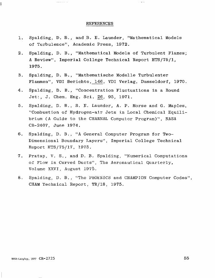
REFERENCES
1. Spalding, D. B., and B. E. Launder, "Mathematical Models of Turbulence", Academic Press, 1972.
2. Spalding, D. B., "Mathematical Models of Turbulent Flames; A Review", Imperial College Technical Report HTS/75/1, 1975.
3. Spalding, D. B., "Mathematische Modelle Turbulenter Flammen", VDI Berichte , 146, VDI Verlag, Dusseldorf, 1970.
4. Spalding, D. B., "Concentration Fluctuations in a Round Jet:, J. Chem. Eng. Sci. 26, 95, 1971.
5. Spalding, D. B., B. E. Launder, A. P. Morse and G. Maples, "Combustion of Hydrogen-air Jets in Local Chemical Equili- brium (A Guide to the CHARNAL Computer Program)", NASA CR-2407, June 1974.
6. Spalding, D. B., "A General Computer Program for Two- Dimensional Boundary Layers", Imperial College Technical Report HTS/75/17, 1975.
7. Pratap, V. S., and D. B. Spalding, "Numerical Computations of Flow in Curved Ducts", The Aeronautical Quarterly, Volume XXVI, August 1975.
8. Spalding, D. B., "The PHOENICS and CHAMPION Computer Codes", CHAM Technical Report, TR/18, 1975.
NASA-Langley, 1977 CR-2725 55