equations of motion with viscosity physical oceanography instructor: dr. cheng-chien liucheng-chien...

Equations of Motion With ViscosityEquations of Motion With Viscosity

Physical oceanographyInstructor: Dr. Cheng-Chien Liu

Department of Earth Sciences

National Cheng Kung University

Last updated: 1 November 2003

Chapter 8Chapter 8

IntroductionIntroduction

FrictionFriction• For most of the interior of the ocean and

atmosphere: Fr 0 negligible

• Boundary layerA thin, viscous layer adjacent to the boundaryNo-slip boundary condition rapid change of velocity

outer boundary velocityFr is non-negligible within the boundary layer

The Influence of ViscosityThe Influence of Viscosity

Molecular viscosityMolecular viscosity• Fig 8.1• Collision between molecules and boundary• Transfer momentum• Inefficient important only within few mms• The kinematic molecular viscosity

= 10-6m2/s for water at 200C

• DefinitionThe ratio of the stress Tx tangential to the boundary of a fluid and the

shear of the fluid at the boundaryTzx = u/z

• Extension to 3D

TurbulenceTurbulence

Reynolds numberReynolds number• the influence of a boundary transferred into the

interior of the flow turbulence• Reynolds experiment (1883)

Fig 8.2V laminar turbulent flowTransition occurs at Re = VD/ 2000Same Re, same flow pattern (Fig 8.3)

• Reynolds number ReThe ratio of the non-linear terms to the viscous terms of the momentum

equationCharacteristic length LCharacteristic velocity U

Turbulence (cont.)Turbulence (cont.)

Turbulent stresses: the Reynolds stressTurbulent stresses: the Reynolds stress• Prandtl and Karmen hypothesized that

Parcels of fluid in a turbulent flow played the same role in transferring momentum within the flow that molecules played in laminar flow

Separate the momentum equation into mean and turbulent components u = U + u' ; v = V + v' ; w = W + w' ; p = P + p'

Turbulence (cont.)Turbulence (cont.)

Equations of motion with viscosityEquations of motion with viscosity• X component

Calculation of Reynolds StressCalculation of Reynolds Stress

By Analogy with Molecular ViscosityBy Analogy with Molecular Viscosity• Fig 8.1

Wind flow above the sea surfaceFlow at the bottom boundary layer in the ocean Flow in the mixed layer at the sea surface

• Steady state/t = /x = /y the turbulent frictional term:

Fx = (-1/) Tz/z = (-/z) <u'w'>

• In analogy with Tzx = u/z-<u'w'> = Tzx = AzU/z Tzx/z = Az2U/z2

Az : the eddy viscosity Az cannot be obtained from theory. Instead, it must be calculated from data collected in

wind tunnels or measured in the surface boundary layer at sea

If the molecular viscosity terms are comparatively smaller

Calculation of Reynolds Stress Calculation of Reynolds Stress (cont.)(cont.)

By Analogy with Molecular Viscosity (cont.)By Analogy with Molecular Viscosity (cont.)• Problems with the eddy-viscosity approach

Except in boundary layers a few meters thick, geophysical flows may be influenced by several characteristic scales

The height above the sea z The Monin-Obukhov scale L discussed in §4.3, and The typical velocity U divided by the Coriolis parameter U / f

The velocities u', w' are a property of the fluid, while Az is a property of the flow

Eddy viscosity terms are not symmetric, <u'v'> = <v'u'> but


From a Statistical Theory of From a Statistical Theory of TurbulenceTurbulence• Relate <u'u'> to higher order correlations of

the form <u'u'u'>• The closure problem in turbulence

determine the higher order terms no general solution

• Isotropic turbulence: turbulence with statistical properties that are independent of direction


Summary: for most oceanic flowsSummary: for most oceanic flows• Ax, Ay, and Az cannot be calculated accurately• Can be estimated from measurements

Measurements in the ocean difficultMeasurements in the lab cannot reach Re =1011

• The statistical theory of turbulence gives useful insight into the role of turbulence in the ocean an area of active research

• Some values for water = 10-6 m2/star at 15°C = 106 m2/s glacier ice = 1010 m2/s Ay = 104 m2/s

The Turbulent Boundary Layer The Turbulent Boundary Layer Over a Flat PlateOver a Flat Plate

The mixing-length theoryThe mixing-length theory• Empirical theory

G.I.Taylor (1886-1975), L. Prandtl (1875-1953), and T. von Karman (1818-1963)

Predicts well U(z) close to the boundary

• U(z) = u*/ ln(z/z0)Assuming: U z Tzx = u/z U = Tzxz/Non-dimensionlizing: U/u* = u*z/

Where u* 2 = Tzx/ is the friction velocity

By analogy with molecular viscosity: Tzx/ = AzU/z = u* 2

Assuming: Az = kzu*

large eddies are more effective in mixing momentum than small eddies, and therefore Az ought to vary with distance from the wall

dU = u*/(kz)dzFor airflow over the sea, k = 0.4 and z0 = 0.0156u*2/g

Mixing in the OceanMixing in the Ocean

MixingMixing• Instability mixing• Vertical mixing

Work against buoyancy need more energyDiapycnal mixingImportant change the vertical structureEquation: /t + W/z = /z(Az/z) + S

: tracer, such as Salt and Temperature Az: the vertical eddy diffusivity

W: mean vertical velocity S: source term

• Horizontal mixingLarger

Average Vertical MixingAverage Vertical Mixing

Observation by Walter Munk (1966)Observation by Walter Munk (1966)• Simple observation calculation of vertical mixing

Thermocline everywhereDeeper part doesn‘t change for decades (Fig 8.4)

steady state balance between

Downward mixing of heat by turbulence Upward transport of heat by a mean vertical current W

Steady state equation without source term: WT/z = /z(AzT/z) Solution: T(z) T0exp(z/H)

H = Az/W: the scale length of the thermocline

T0 = T(z=0)

Simple observation T(z) calculation of vertical mixing H Vertical distribution of C14 Az (1.3 10-4m2/s) and W (1.2 cm/day) H

W the average vertical flux of water through the thermocline 25 ~ 30 Sv of water

Measured Vertical MixingMeasured Vertical Mixing

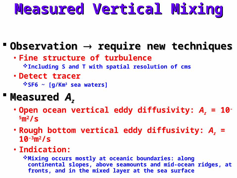
Observation Observation require new techniquesrequire new techniques• Fine structure of turbulence

Including S and T with spatial resolution of cms

• Detect tracerSF6 ~ [g/Km3 sea waters]

Measured Measured AAzz

• Open ocean vertical eddy diffusivity: Az = 10-5m2/s• Rough bottom vertical eddy diffusivity: Az = 10-3m2/s• Indication:

Mixing occurs mostly at oceanic boundaries: along continental slopes, above seamounts and mid-ocean ridges, at fronts, and in the mixed layer at the sea surface

Measured Vertical Mixing (cont.)Measured Vertical Mixing (cont.)

DiscrepancyDiscrepancy• Deep convection meridional overturning

circulationDeep convection may mix properties rather than mass

smaller mass of upwelled water ( 8 Sv)

• Mixing along the boundaries or in the source regionExample: mid Atlantic water Gulf Stream mid

Atlantic

Measured Horizontal MixingMeasured Horizontal Mixing

Horizontal mixing = Horizontal mixing = fnfn((ReRe))• A/ A/ ~ UL/ = Re

: the molecular diffusivity of heatAx ~ UL

Measured Measured AAxx

• Geostrophic Horizontal Eddy Diffusivity: Ax = 8 102 m2/s

• Open-Ocean Horizontal Eddy Diffusivity: Ax = 1 – 3 m2/s

StabilityStability

Three types of instabilityThree types of instability• Static stability (z)

• Dynamic stability velocity shear

• Double-diffusion S, T

Stability (cont.)Stability (cont.)

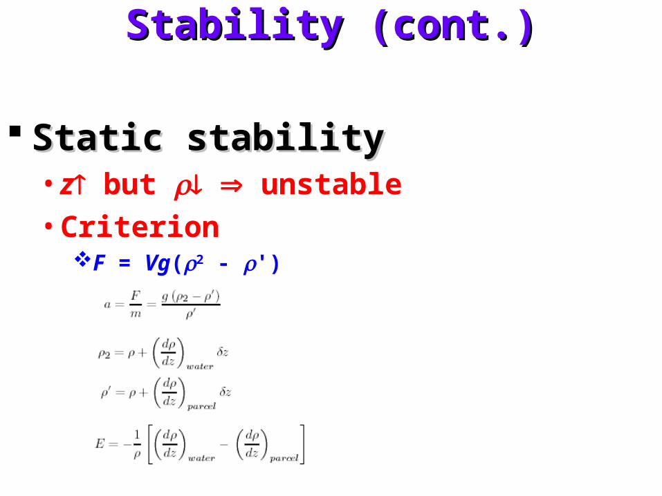
Static stabilityStatic stability• z but unstable

• CriterionF = Vg(2 - ')


Static stability (cont.) Static stability (cont.) • The stability of the water column E -a /(gz)

• More accurate form of E: E(S(z), t(z), z)


Static stability (cont.)Static stability (cont.)• The stability equation

In the upper kilometer of the ocean: (p/z)water >> (p/z)parcel E (-1/)dp/dz (-1/)dt/dz

Below about a kilometer in the ocean, (z) 0 E = E(S(z), t(z), z)

• Stability is defined such thatE > 0 Stable E = 0 Neutral Stability E < 0 Unstable

In the upper kilometer of the ocean, z < 1,000m, E = (50-1000)×10-8/m In deep trenches where z > 7,000m, E = 1×10-8/m


Static stability (cont.)Static stability (cont.)• Stability frequency N

The influence of stability is usually expressed by NN2 -gE N is often called the Brunt-Vaisala frequency or the

stratification frequencyThe vertical frequency excited by a vertical displacement of

a fluid parcelThe maximum frequency of internal waves in the oceanFig 8.5: typical values of N


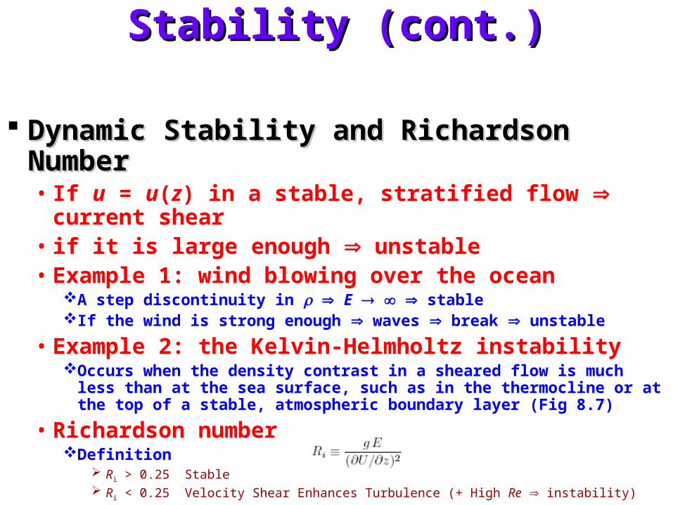
Dynamic Stability and Richardson NumberDynamic Stability and Richardson Number• If u = u(z) in a stable, stratified flow current shear• if it is large enough unstable• Example 1: wind blowing over the ocean

A step discontinuity in E stableIf the wind is strong enough waves break unstable

• Example 2: the Kelvin-Helmholtz instabilityOccurs when the density contrast in a sheared flow is much less than at

the sea surface, such as in the thermocline or at the top of a stable, atmospheric boundary layer (Fig 8.7)

• Richardson numberDefinition

Ri > 0.25 Stable Ri < 0.25 Velocity Shear Enhances Turbulence (+ High Re instability)


Double Diffusion and Salt FingersDouble Diffusion and Salt Fingers• In some regions, as z + no current

unstable?!It occurs because the molecular diffusion of heat is about

100 times faster than the molecular diffusion of salt


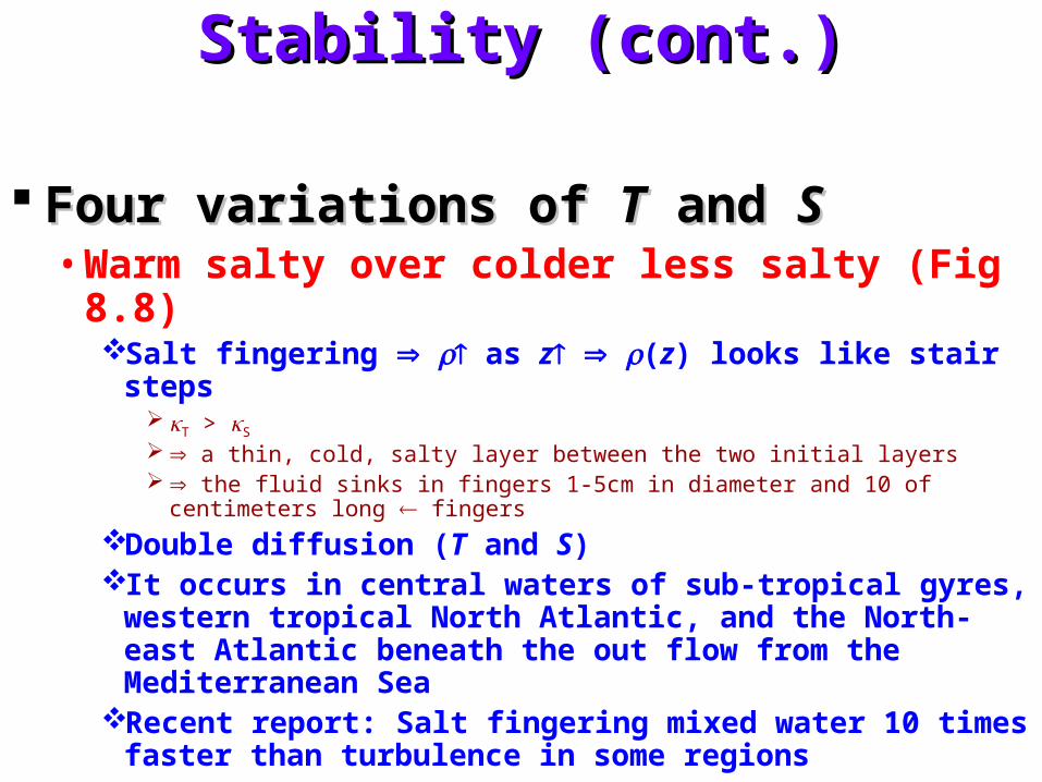
Four variations of Four variations of TT and and SS• Warm salty over colder less salty (Fig 8.8)

Salt fingering as z (z) looks like stair steps T > S

a thin, cold, salty layer between the two initial layers the fluid sinks in fingers 1-5cm in diameter and 10 of centimeters long

fingers

Double diffusion (T and S)It occurs in central waters of sub-tropical gyres, western

tropical North Atlantic, and the North-east Atlantic beneath the out flow from the Mediterranean Sea

Recent report: Salt fingering mixed water 10 times faster than turbulence in some regions


Four variations of Four variations of TT and and SS (cont.) (cont.)• Colder less salty over warm salty

Diffusive convection Double diffusion a thin, warm, less-salty layer at the base of the upper, colder, less-salty layer

and a colder, salty layer forms at the top of the lower, warmer, salty layer sharpen the interface and reduce any small gradients of

Less common than salt fingeringMostly found at high latitudesDiffusive convection also (z) looks like stair steps

• Cold salty over warmer less saltyAlways statically unstable

• Warmer less salty over cold saltyAlways stable and double diffusion diffuses the interface between the

two layers

Important ConceptsImportant Concepts

• Friction in the ocean is important only over distances of a few millimeters. For most flows, friction can be ignored.

• The ocean is turbulent for all flows whose typical dimension exceeds a few centimeters, yet the theory for turbulent flow in the ocean is poorly understood.

• The influence of turbulence is a function of the Reynolds number of the flow. Flows with the same geometry and Reynolds number have the same streamlines

Important Concepts (cont.)Important Concepts (cont.)

• Oceanographers assume that turbulence influences flows over distances greater than a few centimeters in the same way that molecular viscosity influences flow over much smaller distances.

• The influence of turbulence leads to Reynolds stress terms in the momentum equation.

• The influence of static stability in the ocean is expressed as a frequency, the stability frequency. The larger the frequency, the more stable the water column


• The influence of shear stability is expressed through the Richardson number. The greater the velocity shear, and the weaker the static stability, the more likely the flow will become turbulent.

• Molecular diffusion of heat is much faster than the diffusion of salt. This leads to a double-diffusion instability which modifies the density distribution in the water column in many regions of the ocean.

• Instability in the ocean leads to mixing. Mixing across surfaces of constant density is much smaller than mixing along such surfaces


• Horizontal eddy diffusivity in the ocean is much greater than vertical eddy diffusivity.

• Measurements of eddy diffusivity indicate water is mixed vertically near oceanic boundaries such as above seamounts and mid-ocean ridges.

equations of motion with viscosity physical oceanography instructor: dr. cheng-chien liucheng-chien...

Documents