Equations of Gauge TheoryKaren Uhlenbeck

Notes by Laura Fredrickson

These notes are based on a series of lectures Professor Karen Uhlenbeck gave in 2012 atTemple University in Philadelphia. In a series of three lectures, Karen gave a history of theequations of gauge theory, from the Yang-Mills equations to the Kapustin-Witten equations,with a particular eye towards the relationship between the physics and mathematics com-munities. The notes are organized into three chapters, and are oriented towards the futureof the Kapustin-Witten equations.

Chapter 1 discusses Yang-Mills equations, from their origins in the physics literature asa generalization of Maxwell’s equations for electromagnetism to their current applicationin four-manifolds in Donaldson Theory and Floer Theory by providing new topological in-variants. The first chapter discusses a number of real four-dimensional gauge theories, butfocuses on the particularly interesting self-dual Yang-Mills equations. The Kapustin-Wittenequations are a “complexification” (in some sense) of the self-dual Yang-Mills equations.As such, we are interested in which results about the self-dual Yang-Mills equations havecomplex counterparts that are true for the Kapustin-Witten equations.

Chapter 2 discusses Hitchin’s equations, a set of equations over a two-dimensional Rie-mann surface, obtained by dimensional reduction of the self-dual Yang-Mills equations.While the self-dual Yang-Mills equations are a real gauge theory, featuring the real cur-vature of the real connection and real gauge group, Hitchin’s equations are a complex gaugetheory. They are the equations for a flat complex connection with an extra “zero momentmap” condition. The Kapustin-Witten equations are also a complex gauge theory with a zeromoment map condition, so the Kapustin-Witten equations are (in some sense) a particularhigher-dimensional generalization of Hitchin’s equations. In the second chapter, we discussthis mysterious zero moment map condition and the relation between Hitchin’s equationsand representation theory.

Finally, Chapter 3 is about the Kapustin-Witten equations. All the material in the pre-vious two chapters comes together in this chapter. We prove results for the Kapustin-Wittenequations that are the complex counterparts of results for the self-dual Yang-Mills equationsor the higher-dimensional analog of results for Hitchin’s equations. This includes some ana-lytic estimates for solutions of Kapustin-Witten equations that would be the foundation forany topological results derived from the Kapustin-Witten equations.

More than a reference for the equations of gauge, these notes are a story about gaugetheory: how obscure developments launched some of today’s prominent areas of research,how strange and unnatural some of the developments in gauge theory must have appearedat the time, and why mathematicians trust the almost-magical intuition of the physicists.Karen peppered the lectures with stories of her own. To improve the readability, these storiedparts are offset from the mathematical text in italics with wider margins.

These lectures were given at Temple University in Philadelphia, PA between February7-9, 2012 as part of their Emil Grosswald lecture series.

1

Contents

1 The Yang-Mills equations 51.1 Maxwell’s Equations . . . . . . . . . . . . . . . . . . . . . . . . . . . . . . . 5

1.1.1 Invariance under Lorentz transformations . . . . . . . . . . . . . . . . 61.1.2 Maxwell’s equations as an U(1) gauge theory . . . . . . . . . . . . . . 7

1.2 Yang-Mills Equations . . . . . . . . . . . . . . . . . . . . . . . . . . . . . . . 91.2.1 Origins . . . . . . . . . . . . . . . . . . . . . . . . . . . . . . . . . . . 91.2.2 Variational Formulation & self-dual Yang-Mills equations . . . . . . . 111.2.3 The analysis of the Yang-Mills equations . . . . . . . . . . . . . . . . 111.2.4 Donaldson Theory as an application of

the self-dual Yang-Mills equations . . . . . . . . . . . . . . . . . . . . 131.3 Seiberg-Witten Equations . . . . . . . . . . . . . . . . . . . . . . . . . . . . 17

1.3.1 Origins . . . . . . . . . . . . . . . . . . . . . . . . . . . . . . . . . . . 171.3.2 The Equations . . . . . . . . . . . . . . . . . . . . . . . . . . . . . . 181.3.3 Useful Features of Equations . . . . . . . . . . . . . . . . . . . . . . . 181.3.4 Relation to Topology . . . . . . . . . . . . . . . . . . . . . . . . . . . 19

2 Hitchin’s equations 202.1 Origin of Hitchin’s equations . . . . . . . . . . . . . . . . . . . . . . . . . . . 20

2.1.1 Bogomolny Equations from dimensional deduction to R3 . . . . . . . 202.1.2 Hitchin’s equations from dimensional reduction to R2 . . . . . . . . . 22

2.2 Hitchin’s Equations . . . . . . . . . . . . . . . . . . . . . . . . . . . . . . . . 222.3 Moment maps in Hitchin’s equations . . . . . . . . . . . . . . . . . . . . . . 23

2.3.1 Representation Theory . . . . . . . . . . . . . . . . . . . . . . . . . . 242.3.2 The moment map . . . . . . . . . . . . . . . . . . . . . . . . . . . . . 25

2.4 Extensions of Results and Applications . . . . . . . . . . . . . . . . . . . . . 26

3 The Kapustin-Witten equations 283.1 The Kapustin-Witten equations are absolute minimizers of the complex Yang-

Mills functional . . . . . . . . . . . . . . . . . . . . . . . . . . . . . . . . . . 303.2 Zero Moment Map Condition . . . . . . . . . . . . . . . . . . . . . . . . . . 343.3 Applications of the Kapustin-Witten equations . . . . . . . . . . . . . . . . . 34

3.3.1 Relationship between the Kapustin-Witten Equations and other equa-tions . . . . . . . . . . . . . . . . . . . . . . . . . . . . . . . . . . . . 35

3.3.2 Kapustin-Witten Equations on Compact Manifolds . . . . . . . . . . 363.4 Boundary Value Problems in the Kapustin-Witten Equations . . . . . . . . . 37

2

3.5 Non-linear Analysis in the Kapustin-Witten Equations . . . . . . . . . . . . 383.5.1 Bochner-Weitzenbock Formula . . . . . . . . . . . . . . . . . . . . . . 383.5.2 Some Estimates . . . . . . . . . . . . . . . . . . . . . . . . . . . . . . 413.5.3 Difficulties in the Getting Better Estimates . . . . . . . . . . . . . . . 41

3.6 Future Hopes for Kapustin-Witten Equations . . . . . . . . . . . . . . . . . 43

Introduction

The story of the Yang-Mills equations exemplifies the changing relationship between mathe-matics and physics. Before the 1960s there was little collaboration between mathematiciansand physicists. Now there is much collaboration and cross-fertilization between mathematicsand physics, and more generally between math and the other sciences. The entire positionof mathematics within the larger scientific community has changed.

In 1954 the Yang-Mills equations were published in a notable physics journal PhysicalReview, but the equations were not notable at the time either among physicists or mathe-maticians. Not much progress was made on the equations for over a decade because theywere so difficult. Outside of the physics community, in 1963, mathematicians Atiyah andSinger published their Atiyah-Singer Index theorem. This result was spectacularly recog-nized. Using the Index Theorem, mathematicians were able to compute the dimension ofthe moduli space of solutions of these self-dual Yang-Mills equations arising from physics.This was one of the first major results in the study of the Yang-Mills equations.

In 1983, Donaldson used the Yang-Mills equations arising from physics in a purely math-ematical context. Donaldson got new topological invariants for four-manifolds by studyingthe moduli space of solutions of the self-dual Yang-Mills equations over those four-manifolds.Donaldson’s theorem and his method of proof opened up entirely new mathematical vistas.

So why are we mathematicians here? The physicists wrote down the Yang-Millsequations in 1954, and these equations have been employed in a lot of new mathe-matics, launching new fields like four-manifolds and particularly Donaldson The-ory and Floer theory. The physicists in 1954 didn’t even say that these equationswere important!

Now physicists such as Ed Witten and Anton Kapustin are writing down equa-tions and they say they are important. So do we listen to the physicists or not?I’m giving this series of lectures with the thesis that we should.

Timeline of Major Developments in Gauge Theory

• 1954 Yang-Mills equations appear in physics journal

• 1963 Atiyah-Singer Index Theorem

• 1977 Atiyah-Hitchin-Singer: deformations of instantons

3

• 1978 Atiyah-Drinfeld-Hitchin-Manin give a a description of solutions, construction ofinstantons gave a description of the solutions of Yang-Mills equations.

• 1983 Donaldson uses Yang-Mills in 4-manifold topology

• 1983 Atiyah-Bott: Yang-Mills over Riemann surface

• 1983 Hitchin: construction of monopole

• 1986 Connection with algebraic topology

• 1987 Hitchin self-dual equations on a Riemann surface

• 1989 Floer: “Witten’s complex and ∞-dimensional Morse theory”

• 1994-1995 Taubes: Seiberg-Witten theory

• 2006 Preprint on Kapustin-Witten equations

• 2007 Kapustin-Witten equations published

4

Chapter 1

The Yang-Mills equations

1.1 Maxwell’s Equations

The Yang-Mills equations are a glorification of Maxwell’s equations, and consequently weturn our attention first to these. Maxwell’s equations describe the time-evolution of electricand magnetic fields on R3 × R, where R3 is the space and R is the time. Electric chargesand currents generate such electric and magnetic fields.

Let E be an electric field and B′ be a magnetic field. In coordinates dx1, dx2, dx3 onR3 these are given by

E = Ej dxj

B′ = Bj dxj

Here E,B′ ∈ Ω1(R3), but it is preferable to think of the magnetic field as a two-formB = ?B′ ∈ Ω2(R3). 1

1The operator ? indicates the point-wise linear Hodge star operator, dependent on the usual Riemannianmetric on Rn that gives an isomorphism

? : Ωj → Ωn−j .

For any orthonormal basis dx1, . . . dxn, the Hodge star operator is defined by

?(dx1 ∧ dx2 ∧ · · · ∧ dxj) = dxj+1 ∧ · · · ∧ dxn−1 ∧ dxn

Note a few properties of the Hodge star operator:

• ?2 = (−1)(j)(n−j) : Ωj(Rn)→ Ωj(Rn).

• ? is bijective

• The Hodge star defines an inner product on Ω•(M), the vector space of forms on a Riemannianmanifold, M :

〈α, β〉 =

∫M

α ∧ ?β (1.1)

for α, β ∈ Ω•(M,R). Note thatΩ•(M) = ⊕dimM

k=0 Ωk(M)

is a graded algebra, and 〈α, β〉 = 0 unless α and β are in the same grading.

5

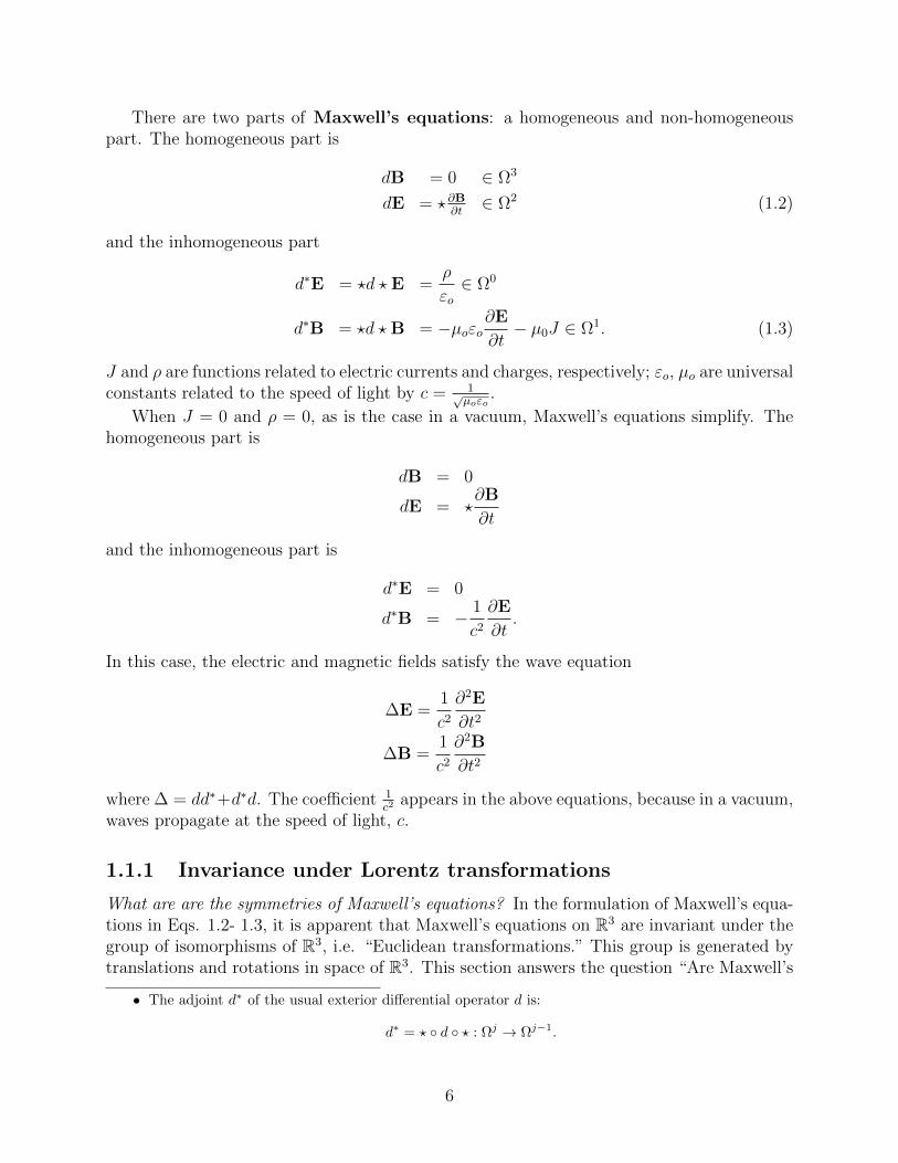
There are two parts of Maxwell’s equations: a homogeneous and non-homogeneouspart. The homogeneous part is

dB = 0 ∈ Ω3

dE = ?∂B∂t∈ Ω2 (1.2)

and the inhomogeneous part

d∗E = ?d ? E =ρ

εo∈ Ω0

d∗B = ?d ?B = −µoεo∂E

∂t− µ0J ∈ Ω1. (1.3)

J and ρ are functions related to electric currents and charges, respectively; εo, µo are universalconstants related to the speed of light by c = 1√

µoεo.

When J = 0 and ρ = 0, as is the case in a vacuum, Maxwell’s equations simplify. Thehomogeneous part is

dB = 0

dE = ?∂B

∂t

and the inhomogeneous part is

d∗E = 0

d∗B = − 1

c2∂E

∂t.

In this case, the electric and magnetic fields satisfy the wave equation

∆E =1

c2∂2E

∂t2

∆B =1

c2∂2B

∂t2

where ∆ = dd∗+d∗d. The coefficient 1c2

appears in the above equations, because in a vacuum,waves propagate at the speed of light, c.

1.1.1 Invariance under Lorentz transformations

What are are the symmetries of Maxwell’s equations? In the formulation of Maxwell’s equa-tions in Eqs. 1.2- 1.3, it is apparent that Maxwell’s equations on R3 are invariant under thegroup of isomorphisms of R3, i.e. “Euclidean transformations.” This group is generated bytranslations and rotations in space of R3. This section answers the question “Are Maxwell’s

• The adjoint d∗ of the usual exterior differential operator d is:

d∗ = ? d ? : Ωj → Ωj−1.

6

equations invariant under the larger group of Lorentz transformations?” which mix timeand space. Since Lorentzian geometry is the geometry of general relativity, this question issynonymous with “Are Maxwell’s equations compatible with general relativity?”

Maxwell’s equations are indeed invariant under Lorentz transformations. However, it isnot at all apparent from Maxwell’s equations, as written in Eqs. 1.2-1.3. Here, we rewriteMaxwell’s equations as equations on Minkowski space R3,1, the Lorentzian manifold withmetric

g = −(cdt)2 + (dx1)2 + (dx2)2 + (dx3)2.

The electric field E ∈ Ω1(R3) and the magnetic field B ∈ Ω2(R3) are combined into atwo-form F known as the electromagnetic field :

F = B + E ∧ dt ∈ Ω2(R3,1). (1.4)

In coordinates x1, x2, x3, t = x0, the electromagnetic field is expressed

F =∑

0≤j<k≤3

Fjk dxj ∧ dxk

where

Fjk =

Ek if j = 0

Bjk if j 6= 0

A simple computation gives Maxwell’s equations in 4-space:

dF = 0 (homogeneous) (1.5)

d∗F = J (inhomogeneous)

where J = (µoJ,ρεo

) is the electrostatic current. In this formulation, it is apparent thatMaxwell’s equations are invariant under Lorentz transformations because the Lorentziantransformations are precisely the isometries of Minkowski space R3,1.

1.1.2 Maxwell’s equations as an U(1) gauge theory

In the previous section, Maxwell’s equations were equations for the electromagnetic fieldF. Here we recast Maxwell’s equations as equations for a quantity A, the electromagneticpotential. It is often more convenient to work with potentials than forces in physics becausepotentials are scalars and forces are vectors. As a scalar, the electromagnetic potentialis more convenient here as well. The electromagnetic potential is defined to be a one-formA ∈ Ω1(R3,1) such that F = dA. Locally, A exists, though it is only unique up to cohomologyclass.

7

The “reality” of the electromagnetic potential A

An important philosophical question in physics is then “To what extent does the electromag-netic potential have reality?” From the discussion in the previous paragraph, certainly anyphysical meaning of A can only depend on the cohomology class [A]. But is the electromag-netic potential just a convenient mathematical construct? Or are there physical consequencesto the electromagnetic potential that do not arise from the electromagnetic field?

The Aharonov-Bohm effect (1959) demonstrates that electromagnetic potential does havephysical meaning. The experimental set up is as pictured in Figure 1.1. An electric current

e-

solenoid

Figure 1.1: Aharonov-Bohm experiment

runs though a solenoid S producing a magnetic field outside in R3−S. This electromagneticfield F vanishes on R3 − S. A beam of electrically-charged electrons is emitted, and themsplit into two topologically distinct beams through the magnetic field on R3 − S, as shown.One beam ψ1 passes through the solenoid, and the other ψ2 does not. The phases of the thetwo beams ψ1 and ψ2 are then compared via interference patterns.

And the phases are different! The phases of the beams are affected by the electromagneticfield, even though that field vanishes where the beams pass. Hence the electromagneticpotential is the truly fundamental quantity.

Gauge theoretic formulation

A theme throughout these lectures is that there were some developments in gauge theorythat were “non-linear.” Rather than proceeding forward in some logical way, there weredevelopments that seemed to be going oddly sideways. In one such critical sideways devel-opment, Maxwell’s equations were reinterpreted as an abelian G = U(1) gauge theory onR3,1 in terms of the electromagnetic potential A. The electromagnetic potential is viewed asa connection on a principle U(1)-bundle over R3,1 and the electromagnetic field F is the cur-vature of that connection. This development will prove to be critical for the generalizationof Yang-Mills that replaces the abelian group G = U(1) with a non-abelian group.

Let P be a principal G-bundle over R3,1. When P is restricted to an open neighborhoodO of R3,1, it is locally isomorphic to O × G. Locally, a connection DA = d + A on P |O is

8

given by A, a g-valued one-form on R3,1. In this case, that means A is locally a iR-valuedone-form. This connection one-form A and the previously defined electromagnetic potentialA are related by

A = iA,

hence the electromagnetic potential A gives a connection DA, defined in coordinates t =x0, x1, x2, x3 by,

DA =3∑

k=0

(∂

∂xk+ Ak

)dxk

The curvature of the connection is given by

FA = (DA)2 =

(∂

∂xjAk −

∂

∂xkAj +

1

2[Aj, Ak]

)dxj ∧ dxk

but in this case, since U(1) is abelian, the Lie bracket is trivial, and

iF = FA = dA

i.e., the curvature of the connection is precisely the electromagnetic field. Consequently, asa gauge theory, Maxwell’s equations are simply:

DAFA = d2A = 0 (1.6)

D∗AFA = d∗dA = J .

Note that the homogeneous equation is satisfied by any connection since d2 = 0. The differ-ential operator d∗d looks similar to the Laplacian on forms, ∆ = d∗d+dd∗, the quintessentialelliptic operator. We point this out here because in the different gauge theories in subsequentsections, this ellipticity will play a crucial role in the analysis.

1.2 Yang-Mills Equations

1.2.1 Origins

The innovation of Yang-Mills was to replace the abelian group G = U(1) appearing inMaxwell’s equations with a non-abelian group, consequently obtaining a non-abelian gaugetheory, known as Yang-Mills gauge theory. In this sense, the Yang-Mills equations are aglorification of Maxwell’s equations.

Yang-Mills replaced the Lie algebra associated to the abelian Lie group U(1) with the Liealgebra associated to the compact non-abelian Lie group SU(2).2The Yang-Mills equationson R3,1, like Maxwell’s equations, are given in terms of a connection DA. Locally, theconnection DA = d+ A is given by an su(2)-valued one-form

A = Ajdxj Aj ∈ su(2).

2Here it is not the particular choice of Lie group SU(2) that matters, but rather the shift from an abelianto non-abelian Lie group. It is in this that all the difficulties immediately arise. One could instead take thenon-abelian Lie group E8 instead, for example.

9

The curvature FA is locally a su(2)-valued two-form expressed by

FA = (DA)2 = dA+1

2[A,A]3.

The equations are

DAFA = 0

D∗AFA = J .

(When G = U(1), these equations are just Maxwell’s equations. These same equationsappeared in Eq. 1.6. ) The homogeneous equation DAFA = 0 is known as Bianchi identity,and is true for all connections.The inhomogeneous part is

D∗AFA = J

for J ∈ Ω(R3,1, su(2)). We will take J = 0 for simplicity. The Yang-Mills equations areinvariant under the infinite-dimensional group of gauge transformations

G = g : M → G,

which acts on a connection DA = d+ A by conjugation

g · (d+ A) = g(d+ A)g−1 = −dgg−1 + gAg−1.

Modulo these gauge transformations, the Yang-Mills equations are elliptic!

The Yang-Mills equations

DAFA = 0 (1.8)

D∗AFA = 0.

can be defined for a connection on a principle G-bundle, P, over any smooth Riemannian4-manifold M .

How did the Yang-Mills equations go from being equations on the non-compact Lorentzianmanifold R3,1 to equations on compact Riemannian manifolds? This is yet another develop-ment in gauge theory that was not “linear.” The base space changed from the Lorentzianmanifold R3,1 to the Riemannian manifold R4 via Wick rotation. However, there was littleimmediate advantage in this.

3Here [ · , · ] refers to the usual extension of the Lie bracket on g = su(2) to Ω1(O, g) defined by takingthe wedge of the basis 1-forms and the brackets of the g-valued coefficients. In coordinates,

[Aidxi, Bjdx

j ] = [Ai, Bj ]dxi ∧ dxj (1.7)

10

1.2.2 Variational Formulation & self-dual Yang-Mills equations

The Yang-Mills equations are the Euler-Lagrange equations for theYang-Mills functional

Ym(DA) =

∫M

|FA|2dvol :=

∫M

tr(FA ∧ ?F ∗A)dvol (1.9)

The inner product appearing in the above equation is described in footnote 4. The proofthat the Yang-Mills equations are the Euler-Lagrange equations is, similarly in footnote

There is a special class of solutions to the Yang-Mills equations that will be our focus laterin this chapter. These are the connections which satisfy the (anti-)self-dual Yang-Millsequations

FA = ± ? FA. (1.10)

Any solution of the (anti-)self-dual Yang-Mills equations is also a solution of the Yang-Millsequations. But more than that, solutions of the (anti-) self-dual Yang-Mills equations areabsolute minima of the Yang-Mills functional. The proof of this fact is delayed until Chapter3 Proposition 3.1.1 because there is a similar statement that is true of the Kapustin-Wittenequations.

1.2.3 The analysis of the Yang-Mills equations

From the time the Yang-Mills equations appeared in a physics journal in 1954, a handful ofphysicists were interested in studying single solutions of the Yang-Mills equations (known asinstantons) on the Lorentzian manifold R3,1, as well as the space of such solutions. However,the equations were difficult to work with, and little progress was made for over ten years.

The next major development in the story of the so-far-only-physicist’s Yang-Millsequations was one by mathematicians! The Atiyah-Singer Index Theorem saidsomething about the dimension of the space of solutions to the Yang-Mills equa-tions. The mathematicians had something to say to the physicists, and it is rightat this point that the relation between the mathematics and physics communitybegan to change. It is here that the cooperation and cross-fertilization really be-gan.

I don’t know how to describe the tremendous difference this made. The entireposition that mathematics held within the scientific community changed. Themathematicians actually had something to say!

4The inner product on Ω•(M,P ×G g) comes from the invariant inner product on g defined by

< A,B >su(n)= tr(AB∗)

and the inner product on Ω•(M) defined via the Hodge star

< α, β >Ω•(M)=

∫M

α ∧ ?β.

11

Of all the properties of the moduli space of solutions, the dimension of the moduli space isone of the easiest properties. However, determining even this easiest property of the modulispace of self-dual Yang-Mills equations requires the heavy machinery of the Atiyah-Singerindex theorem and technical implicit-function-theorem-type arguments. After discussing theAtiyah-Singer Index Theorem in Section 1.2.3, we turn in Section 1.2.3 to the tools availablefor proving other properties about the moduli space of solutions of the self-dual Yang-Millsequations.

The Atiyah-Singer Index Theorem

The Atiyah-Singer Index Theorem(1963) is a remarkable theorem about elliptic differentialoperators on compact manifolds, relating the analytical index of the operator (which is turnis related to the dimension of the space of solutions) to the topological index (defined purelyby topological data.)

We briefly rehearse the modifications of the Yang-Mills equations we described in theprevious sections, since they are essential for the application of the Atiyah-Singer IndexTheorem to the Yang-Mills equations. First, the Yang-Mills equations became equations onR4 rather than R3,1. (None of the analysis works right in R3,1!) Second, we replaced the non-compact base manifold R4 with the compact space S4 = R4 ∪ ∞, or, in fact, any compact4-manifold M4. The last, and perhaps strangest, modification is the switch from consideringthe full Yang-Mills equations to the self-dual Yang-Mills equations. This modification isstrange because the full Yang-Mills equations have some nice properties: they are alreadyelliptic, and, unlike the self-dual Yang-Mills equations, the full Yang-Mills equations are theEuler-Lagrange equations for a variational problem.

The Atiyah-Singer Index Theorem will tell us something about the hypothetical dimen-sion of the moduli space of solutions M to the self-dual Yang-Mills equations

M = DA

∣∣∣ ? FA = FA/G.

on a principle bundle P over M4. The hypothetical dimension is computed from the topo-logical index, which is related to the topology of the principle bundle P .

For G = SU(2), principle SU(2)-bundles on M4 are classified by their second Chern classc2(P ) ∈ H4(X,Z) = Z, an integer topological invariant. For the sphere S4, we can explicitlystate what the second Chern class c2(P ) is measuring. The bundle over S4 is constructedfrom trivial bundles over two patches: S4 − ∞ and B∞, a ball around ∞; and a gluingmap, possibly twisting the bundle, on the intersection. This gluing map is

φ : S4 − ∞ ∩B∞ → SU(2).

The domain S4 − ∞ ∩ B∞ deformation retracts to S3 and the Lie group SU(2) is topo-logically S3, so the gluing map φ gives a map

φS3 : S3 → S3,

and the degree of this map is the exactly second Chern class c2(P ) of the bundle P.

12

The Atiyah-Singer Index Theorem says the following about the dimension of the modulispace:

Theorem 1.2.1 Let P be a principle SU(2)-bundle over M4 and let c2(P ) be the above topo-logical invariant. Then, the moduli space of self-dual instantons has hypothetical dimension

dim(Mk) = 8c2(P )− 3 (1.11)

For S4, this hypothetical dimension is realized.

Tools for Analysis of Yang-Mills

We now turn our attention to the analysis of solutions of self-dual Yang-Mills equations inR4. What tools are available? Here, there is not just one way to do it!

• Twistor theory In R4, you have twistor theory which transforms questions aboutpartial differential equations into questions in complex geometry. Here, the anti-self-dual condition on connections over R4 is turned into a question about holomorphicbundles on the twistor space CP3.

• Algebraic geometry

• Non-linear PDE

What’s interesting about the theory is that non-linear PDE that has been the mostsuccessful and the richest. Of all these approaches–algebra, algebraic geometry,–the non-linear PDE has been richest and most useful. Take this with a grain ofsalt because non-linear PDE is what I do! But I still think if you look at thehistorical record, this is justified.

1.2.4 Donaldson Theory as an application ofthe self-dual Yang-Mills equations

We now turn towards an application of the self-dual Yang-Mills equations in mathematics.In the process, we will be able to say more about the moduli space of instantons. Donaldsonproved a remarkable theorem regarding the topology of 4-manifolds. He proved the existenceof non-smoothable topological 4-manifolds using the topology of the self-dual Yang-Millsequation. He exploited the interaction between the topology of the underlying manifold M4

and the topology of the resulting moduli space of self-dual connections M on a particularprinciple bundle over M . He used remarkable proof techniques that mathematicians hopecan be extended to use in the complex Kapustin-Witten equations discussed in Chapter 3.

Developments in 4-manifold topology prior to Donaldson’s Theorem

Before we turn our attention to Donaldson’s theorem, we briefly describe the developmentsin four-manifold topology before Donaldson’s theorem. Before 1980, people knew very littleabout 4-manifold topology and had few examples of 4-manifolds.

13

I was at the Institute for Advanced Study in Princeton in 1979-1980. Shang cameand gave a talk about four manifolds, and he discussed what people knew about4-manifold topology. I came away from the talk with the realization that peopledidn’t know much about four manifolds. They didn’t know many examples. Theydidn’t know how to work with them. They didn’t know much at all.

Now, shortly after, in 1981, Mike Freedman proved a very important theorem in 4-manifoldtopology about the connection between 4-manifold topology and the classification of non-degenerate quadratic forms (equivalently, non-degenerate symmetric bilinear forms) over theintegers. These non-degenerate quadratic forms are quite rare! From any 4-manifold M4, onenaturally obtains a quadratic form known as the associated bilinear form from the integralsecond cohomology class H2(M4,Z), as follows:

Q : H2(M4,Z)×H2(M4,Z) −→ Z

Q : ([α], [β]) 7→∫M4

α ∧ β. (1.12)

Example Here are some examples of simply-connected 4-manifolds and their associatedbilinear forms:

S4 H2(S4) = 0 Q = 0CP2 H2(CP2) = Z Q =

(1)

S2 × S2 H2(S2 × S2) = Z2 Q =

(0 11 0

)K3 H2(K3) Q = 2E8 + 3Q0

Freedman proved the converse: there is a 4-manifold associated to any non-degeneratequadratic form.

Theorem 1.2.2 (Freedman) For any non-degenerate bilinear form Q over Z there exists asimply-connected topological (but not necessarily smooth!) manifold whose second homologyrealizes this form, i.e. the associated bilinear form to M is Q.

Remark Freedman did not prove uniqueness. In fact, there is exactly one or two suchmanifolds. The extra piece of data to uniquely determine the manifold up to homeomorphismis the Kirby-Siebenmann obstruction in Z/2.

This drastically expanded the number of examples of 4-manifolds mathematicians knew!

14

Donaldson’s Theorem

Building on the work of Freedman, in 1983 Simon Donaldson, a graduate student of Atiyahat the time, proved a remarkable theorem.

What’s the advantage of being a grad student? Well, if you don’t know it’s animpossible theorem, you might actually prove it! Donaldson was messing aroundwith all this impossible stuff, and, lo and behold, he proved something!

Theorem 1.2.3 (Donaldson) Let M4 is a smooth, compact, connected, simply-connected4-manifold, with the property that the associated bilinear form Q is positive-definite (i.e.b− = 0). Then Q is diagonalizable over the integers to the identity matrix. In particular, ifQ is also negative-definite (i.e. b+ = 0), then M = S4.

Donaldson’s theorem implies that many of the of topological 4-manifolds that Freedmanproduced had no differentiable structure.

This not only a startling theorem, given that people didn’t know anything aboutfour-dimensional topology at this point; but the method of proof is extremely as-tonishing and opened a whole new world!

Donaldson’s proof is based on the topology of the space of self-dual Yang-Mills connec-tions on a principle SU(2) bundle over M4, a smooth, compact, simply-connected 4-manifold.Here we sketch the method of proof:

Sketch of Proof Let M4 satisfy the hypothesis of the theorem with associated bilinearform Q and fix a smooth Riemannian structure on M4. There is (up to isomorphism) aunique principle SU(2)-bundle P over M4 with second Chern class c2(P )[M4] = −1.

Consider the moduli spaceM of self-dual connections on P . What doesM look like? Bythe Atiyah-Singer Index Theorem, since c2(P ) = −1, dimM = 5. From the work of Atiyah,M is orientable. M is non-compact, but the non-compact part looks like M4 × (0, 1). Themoduli space also has singularities that look like cones on CP2. These singularities occur atthose self-dual connections which are reducible to U(1)-connections.

Consequently, the moduli space is an oriented cobordism from M4 to⊔nP

CP2, wherenP is the number of reducible connections. The signature σ = (b+, b−), coming from thebilinear form Q, is an oriented cobordism invariant, so

(b+, 0) = σ (M) = σ

(⊔nP

CP2

)= (nP , 0).

It turns out that the reducible connections correspond to α ∈ H2(M ;Z) such that Q(α, α) =1, and the cobordism shows that the number of these reducible connections is equal to thefull rank of the bilinear form Q. Hence, Q is diagonalizable.

15

CP2

CP2

CP2

M4

Figure 1.2: The moduli space of self-dual Yang-Mills connections

Ingredients in Donaldson’s method of proof

Here, we list the ingredients in Donaldson’s proof. Why? Later, we’ll look at the Kapustin-Witten equations, a complex version of the real Yang-Mills equations, and an active areaof research. It would be desirable to generalize the kind of mathematics that appears inDonaldson’s proof to get results in this new complex setting.

Theory of principle bundles This is the basic underlying theory. At the time it wasn’tvery well known, but now it is a classical subject known by many.

Infinite dimensional topology : You need an infinite-dimensional version of Sard’s the-orem.

Finite dimensional topology : Need de Rham theory

Atiyah-Singer Index Theorem : This is necessary to compute dimension of M. Morethan that, the Atiyah-Singer theory is crucial background because it introduced thecrucial notion of Fredholm operator between function spaces, something Donaldson’smethod of proof relies on.

Non-compactness results : The manifold M is not compact. One needs to answer thequestion “Where does non-compactness come from?”

Orientation on M for cobordism.

non-linear PDE : As stated above, need the concept of a Fredholm operator. The Sobolevspaces are the right spaces to work in and we need some analytical results

• Need estimates

• Need genericity properties

16

• Need constructions using gluing procedures: Donaldson used Taubes’ Gluing The-orem, a powerful analytic result, to construct solutions by taking a flat connectionand gluing in singularities at a point. This is a non-linear generalization of howone can add two local solutions of a linear PDE to obtain a global solution. Hereone patches together a solution to a non-linear equation in one region and a solu-tion to a non-linear equation in another region into a global solution by perturbingthe resulting solution using the Implicit Function theorem. This was a method ofsolving equations that was largely unexplored before gauge theory.

Besides the specific topics mentioned, the global analysis of the 1960s is at the basis ofthe entire framework. Given a non-linear elliptic operator on a underlying space, thesolutions form manifold. In global analysis the the interaction between the topologyof these solution manifolds and the topology of the underlying manifold was studied.

Donaldson Theory

Donaldson’s theorem was the first result in an area now known as Donaldson Theory whichgives topological constraints on 4-manifolds using the gauge theoretic self-dual Yang-Millsequations. Donaldson theory is difficult because the self-dual Yang-Mills are not easy toperturb in a gauge invariant way. In the next section, we introduce a set of equationsthat is easier to perturb and, similar to Donaldson Theory, gives topological constraints on4-manifolds.

1.3 Seiberg-Witten Equations

In this section we briefly introduce the Seiberg-Witten equations, another set of equationsthat gives a lot of 4-dimensional topological invariants. The Seiberg-Witten equations area technically easier set of equations to use than the self-dual Yang-Mills equations becausethey are an abelian gauge theory; and it is easier to make deformations in an abelian gaugetheory!

1.3.1 Origins

In 1992, Ed Witten gave a talk at Harvard and Cliff Taubes was in the audience.After the talk Taubes walked up to talk with Witten. Witten told Taubes aboutsome equations, the Seiberg-Witten equations, that he suspected that contained allthe topological 4-manifold invariants that Donaldson theory was extracting fromthe self-dual Yang-Mills equations. Taubes went home and wrote his shortestpaper–just over 15 pages!– on that.

So a physicist walks up to a you as a mathematician, and says “You should bedoing this,” then you go home and it works! And you have no idea why it worksor why you should be doing it. We have 30 years of this pattern. Somehow thephysicists know the interesting equations!

17

What are the Seiberg-Witten equations and why are they so magical? The magic of theSeiberg-Witten equations is that they are an abelian gauge theory with an exterior fieldφ vaguely referred to as a Higgs field. It is surprising that an abelian gauge theory couldcontain the information of the self-dual Yang-Mills equations, with non-abelian structuregroup SU(2). However, one does not obtain such an interesting abelian gauge theory inthe naive way of choosing an abelian gauge group. For example, the G = U(1) Yang-Millsequations are just Maxwell’s equations and one gets nothing except de Rham cohomology.

1.3.2 The Equations

The Seiberg-Witten equations are an abelian gauge theory with gauge group G = U(1). Thedata consequently includes some principal U(1)-bundle with connection DA with curvatureFA. The interest comes from the coupled exterior field φ, known as the Higgs field or spinorfield. Coupling involves nothing more than writing an equation involving both the gaugefield and the Higgs field.

Let M be a smooth oriented Riemannian 4-manifold with SpinC structure and let P bea principle SpinC(4) bundle. The data of the Seiberg-Witten equations is a connection A ona certain line bundle L and a section φ of a certain C2 bundle, known as the spinor field.Let φ be a spinor and A a U(1)-connection on L. The Seiberg-Witten equations are:

FA + φTφ = 0 (1.13)

6DAφ = 0

where 6DA is a Dirac operator and φTφ is some particular sesquilinear map. A solution to theSeiberg-Witten equations is called a monopole. This is a general term for a solution of afirst-order coupled equation. Consequently, solutions of the λ = 0 Bogomolny and Kapustin-Witten equations, which we will introduce in Chapter 2 and 3 respectively, are also calledmonopoles.

1.3.3 Useful Features of Equations

Because the Seiberg-Witten equations are an abelian gauge theory, we can globally fix thecoordinates and take d∗A = 0 globally.

Moreover, the Seiberg-Witten equations are easy to perturb. The curvature FA is Lie-algebra valued two-form, but when G = U(1), because u(1) = iR,

FA ∈ Ω2(M, gP ) ∼=√−1Ω2(M,R).

Consequently FA can be perturbed by adding any self-dual two-form ω. Adding a parameterλ, one obtains a family of perturbed equations:

FA + φTφ+ iλω = 0 (1.14)

6DAφ = 0.

Letting λ→∞, one gets explicit type of solutions that concentrate in different ways.

18

1.3.4 Relation to Topology

Taubes exploited this method of perturbation in his papers. This process of using theSeiberg-Witten equations to get topological information was spectacularly successful. Stilla great deal of 4-manifold topology is based on this.

How do topologists use these deep and beautiful analytical results? They first turnthem into a combinatorial machine.

Before I did gauge theory, I was involved in minimal surfaces. Back in the 1970s,minimal surfaces were used to prove results about 3-manifolds. Well, the firstthing the topologists did was they replaced the beautiful theory of minimal sur-faces with combinatorics. How did they do this? Well the three manifolds havegeometric structure, so you concentrate this structure at the edges of your mani-fold.

For 4-manifolds, I asked Peter Osratch, “Do you really use PDE anymore?” andhe said, “No.” All this PDE stuff has been replaced by combinatorial jazz.

Though Witten suspected Seiberg-Witten theory had all the information of Donaldsontheory, it turns out that Donaldson theory has more information. Both are still activeareas of research. Generally, mathematicians are more interested in Seiberg-Witten theorybecause it is easier to work with. The physicists prefer the self-dual Yang-Mills equations tothe Seiberg-Witten equations. Provided their intuition is correct–as it historically seems tobe– there is still a lot of untapped topological information in the Yang-Mills equations.

19

Chapter 2

Hitchin’s equations

In the previous chapter we saw that a lot of interesting equations have arisen from physicsand string theory in particular. This, in turn, has generated a ton of mathematics. Our goalis to generate some more equations. We will do this is by dimensional reduction.

In this chapter we consider Hitchin’s equations which Hitchin originally called “the self-dual equations on a Riemann surface” in his seminal 1987 paper. We say that Hitchin’sequations are a “complex theory” because they are equations on a complex manifold. TheKapustin-Witten equations, which we will discuss in the third chapter, are also complexequations. Consequently, many aspects that we’ll discuss for Hitchin’s equations, like thezero moment map condition and the relation between solutions of Hitchin’s equations andrepresentation theory, will appear again in the third chapter.

2.1 Origin of Hitchin’s equations

Hitchin’s equations are the self-dual equations on a Riemann surface. They are obtainedby dimensionally reducing the self-dual Yang-Mills equations FA = ?FA on R4 to R2. Af-ter introducing complex coordinates and proving the conformal invariance of the resultingequation on R2, the Hitchin’s equations can be defined on a Riemann surface. Here wedimensionally reduce in two steps: first, from R4 to R3 and obtain the Bogomolny equation;then, dimensionally reduce again to R2 to obtain Hitchin’s equations on R2. We can thenwrite Hitchin’s equations for a Riemann surface. Note that this dimensional reduction is notthe naive dimensional reduction where one simply throws away a dimension. This naive di-mensional reduction to 2 or 3-dimensions doesn’t lead to any interesting equations–only thatFA = 0. In contrast, in the Hitchin’s equations, though we end up with a two-dimensionaltheory by dimensional reduction, we are still studying the self-dual Yang-Mills equations infour dimensions.

2.1.1 Bogomolny Equations from dimensional deduction to R3

Let A ∈ Ω1(R4, su(2)) . In local coordinates,

A = A1dx1 + A2dx

2 + A3dx3 + A4dx

4

20

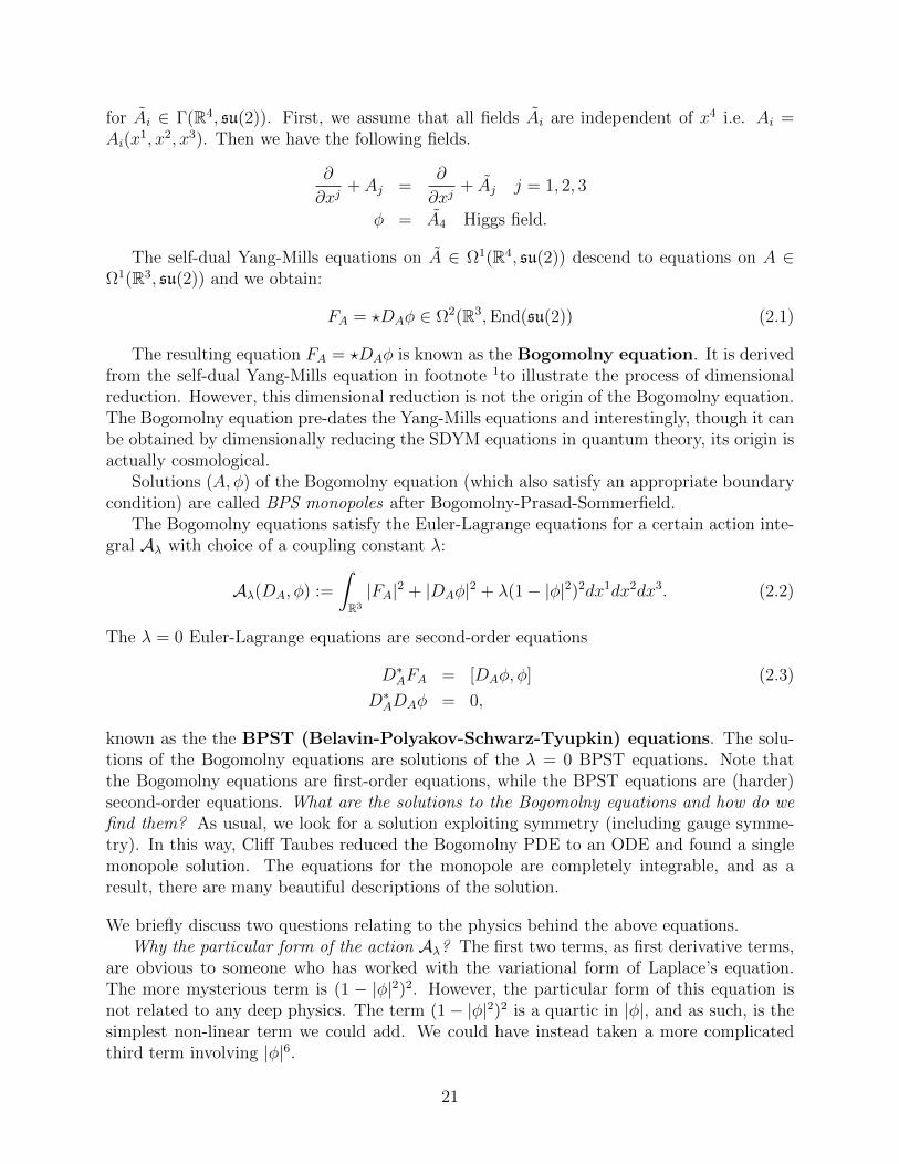
for Ai ∈ Γ(R4, su(2)). First, we assume that all fields Ai are independent of x4 i.e. Ai =Ai(x

1, x2, x3). Then we have the following fields.

∂

∂xj+ Aj =

∂

∂xj+ Aj j = 1, 2, 3

φ = A4 Higgs field.

The self-dual Yang-Mills equations on A ∈ Ω1(R4, su(2)) descend to equations on A ∈Ω1(R3, su(2)) and we obtain:

FA = ?DAφ ∈ Ω2(R3,End(su(2)) (2.1)

The resulting equation FA = ?DAφ is known as the Bogomolny equation. It is derivedfrom the self-dual Yang-Mills equation in footnote 1to illustrate the process of dimensionalreduction. However, this dimensional reduction is not the origin of the Bogomolny equation.The Bogomolny equation pre-dates the Yang-Mills equations and interestingly, though it canbe obtained by dimensionally reducing the SDYM equations in quantum theory, its origin isactually cosmological.

Solutions (A, φ) of the Bogomolny equation (which also satisfy an appropriate boundarycondition) are called BPS monopoles after Bogomolny-Prasad-Sommerfield.

The Bogomolny equations satisfy the Euler-Lagrange equations for a certain action inte-gral Aλ with choice of a coupling constant λ:

Aλ(DA, φ) :=

∫R3

|FA|2 + |DAφ|2 + λ(1− |φ|2)2dx1dx2dx3. (2.2)

The λ = 0 Euler-Lagrange equations are second-order equations

D∗AFA = [DAφ, φ] (2.3)

D∗ADAφ = 0,

known as the the BPST (Belavin-Polyakov-Schwarz-Tyupkin) equations. The solu-tions of the Bogomolny equations are solutions of the λ = 0 BPST equations. Note thatthe Bogomolny equations are first-order equations, while the BPST equations are (harder)second-order equations. What are the solutions to the Bogomolny equations and how do wefind them? As usual, we look for a solution exploiting symmetry (including gauge symme-try). In this way, Cliff Taubes reduced the Bogomolny PDE to an ODE and found a singlemonopole solution. The equations for the monopole are completely integrable, and as aresult, there are many beautiful descriptions of the solution.

We briefly discuss two questions relating to the physics behind the above equations.Why the particular form of the action Aλ? The first two terms, as first derivative terms,

are obvious to someone who has worked with the variational form of Laplace’s equation.The more mysterious term is (1 − |φ|2)2. However, the particular form of this equation isnot related to any deep physics. The term (1− |φ|2)2 is a quartic in |φ|, and as such, is thesimplest non-linear term we could add. We could have instead taken a more complicatedthird term involving |φ|6.

21

How big is λ for cosmologists? The action Aλ(DA, φ) has some cosmological meaning,and so it makes sense to ask what λ is to cosmologists. Cosmologists are looking in universefor a very very very small but non-zero constant λ. In other words, the solutions of theBogomolny equation (a dimensional reduction of the self-dual Yang-Mills equations) aresolutions of the λ = 0, but these are not are not actually what the cosmologist are actuallylooking for in the universe, though they are very close to it.

2.1.2 Hitchin’s equations from dimensional reduction to R2

In the previous section, we saw that dimensional reduction from R4 to R3 produced theinteresting Bogomolny equations. Let’s keep going and dimensionally reduce to R2!

Again, we started with A our full connection on R4.

A =4∑i=1

Aidxi.

In the previous section, to dimensionally reduce to R3, we assumed that everything wasinvariant in the x4 coordinate, Now, to dimensionally reduce to R2, we assume everythingis invariant in both x3 and x4. Now, in addition to a connection A, we also get two Higgsfields, φ1 and φ2:

∂

∂xj+ Aj =

∂

∂xj+ Aj j = 1, 2

φ1 = A3

φ2 = A4

We package the two fields, φ1 and φ2, into a single Higgs field φ, and obtain the followingobjects:

A = A1dx1 + A2dx

2 ∈ Ω1(R2, su(2))

φ = φ1dx1 + φ2dx

2 ∈ Ω1(R2, su(2))

2.2 Hitchin’s Equations

The dimensional reduction of FA = ?FA produces Hitchin’s equations on a R2:

FA −1

2[φ, φ] = 0 (2.4)

DAφ = 0 (2.5)

D∗Aφ = 0 (2.6)

More generally, these equations can be defined on a Riemann surface after introducingcomplex coordinates and proving conformal invariance. Because of their origin, Hitchinoriginally called these equations the “self-dual equations on a Riemann surface.”

22

The moduli space of solutions of Hitchin’s equations is

M(Σ, G) =

(A, φ)

∣∣∣FA− 12[φ,φ]=0

DAφ=0D∗Aφ=0

/G (2.7)

where G is the group of real gauge transformations, i.e. automorphisms of the principalbundle P .

Tools for studying solutions of Hitchin’s equations

Hitchin’s equations are completely integrable! Consequently, they can be approached usingtwistor theory, which was developed exactly for this situation. Other approaches includealgebraic geometry and non-linear PDE. Hitchin described the moduli space using algebraicgeometric methods in his original paper. Of all these tools, non-linear PDE hasn’t been usedas much. However, non-linear PDE seems to be precisely the right tool to understand thenoncompact part of the moduli space.

2.3 Moment maps in Hitchin’s equations

One important interpretation of Hitchin’s equations is that they are the equations for acomplex flat connection with a zero moment map condition.

The equations for a complex flat connection are:

0 = FA+iφ = FA −1

2[φ, φ] + iDAφ

The real and imaginary parts of the equation FA+iφ are the following two of three equationsin Hitchin’s system of equations.

Re(FA+iφ) = FA − 12[φ, φ] = 0

Im(FA+iφ) = DAφ = 0

The equation we’re missing, D∗Aφ = 0 is related to the zero moment map condition.Consequently, one can see that given a solution of Hitchin’s equations (A, φ), we get a

complex flat connection DA+ iφ. This map from solutions of Hitchin’s equations to complexflat connections also works up to gauge equivalence. We have a map of moduli spaces

(A, φ)∣∣∣FA− 1

2[φ,φ]=0

DAφ=0D∗Aφ=0

/G →

A+ iφ

∣∣∣FA+iφ = 0 i.e. FA− 12[φ,φ]=0

DAφ=0

/GC.

Somewhat surprisingly, Hitchin proved that this map above is actually an isomorphism.

Theorem 2.3.1 (Hitchin) We have the following correspondence:(A, φ)

∣∣∣FA− 12[φ,φ]=0

DAφ=0D∗Aφ=0

/G ∼=

A+ iφ

∣∣∣FA+iφ = 0 i.e. FA− 12[φ,φ]=0

DAφ=0

/GC

23

On the right hand side of the correspondence, the larger complex gauge group compensatesfor the missing third equation D∗Aφ = 0. The space on the right is interpreted as themoduli space of flat complex connections. In the next section (Section 2.3.1)we explainthe connection between Hitchin’s equations and representation theory. This comes fromcorrespondence between flat complex connections over Σ and representations ρ : π1(Σ, GC)of the fundamental group of Σ.

The space on the left, the Hitchin moduli space, is better for analysis. The group ofcomplex gauge transformations do not fix the norms. And you can’t have varying normswith PDE! Thus, real gauge theories are necessary for analysis. In Section 2.3.2, we discussthe zero moment condition and how the proof of the correspondence works. Particularly, wediscuss how the equation D∗Aφ allows us to reduce from a complex gauge theory to a realgauge theory.

2.3.1 Representation Theory

For any group G′ and any manifold M , there is a correspondence between flat G′-connectionsover M and representations π1(M) → G′. In the context of Hitchin’s equations, we arelooking at flat complex connections (G′ = GC = SL(2,C)) over a Riemann surface Σ.

From flat connections to representations: Let PC →p Σ be a principal GC-bundle with flatconnection ∇. We get a representation as follows. Pick a base point x0 ∈ Σ. We’ll constructa representation

ρ : π1(Σ, x0)→ GC

For any [γ] ∈ π1(Σ, xo), choose a point γ(0) ∈ p−1(x0) = PC,x0 , the fiber of PC over x0.γ lifts to a unique flat section, γ : [0, 1] → Σ, of PC starting at γ(0). The representation

flat connection

Figure 2.1: Getting a representation

ρ(γ) ∈ π1(Σ, x0) is defined to be the difference of the endpoints of γ i.e.

γ(1) = ρ(γ)γ(0)

24

This is known as the monodromy representation of the connection.We made a few choices defining the representation

ρ : π1(Σ, x0)→ GC.

We chose a path γ in the class of [γ] ∈ π1(Σ, x0). The resulting representation does notdepend on the choice here precisely because the connection is flat. Second, we choose astarting point γ(0). Since we are only interested in the difference of γ(0) and γ(1), therepresentation ρ does not depend on this choice either. Lastly, we chose a base point x0 ∈ Σ.This does change the representation! Changing the base point changes the representationby conjugation. Consequently, we get a well-defined map from flat connections to conjugacyclasses of representations

ρ : π1(Σ, x0)→ GC /GC.

From representations to flat connections:Given ρ : π1(Σ, x0)→ GC, we can construct a bundle with flat connection as follows:Let Σ be the universal cover of Σ. Consider the trivial bundle

Σ×GC → Σ

with flat connection ∇ = d, where d is the ordinary exterior derivative on Σ that doesn’t seethe GC-component.

To get a bundle on Σ, take this flat bundle upstairs, then twist it up and glue it togetherusing the representation ρ.

Σ×GC/(x, g) ∼ (γ · x, ρ(γ)g)

When the bundle is twisted up, the flat connection is twisted too.In the same neighborhood of x0 on Σ, the flat connection may look looks like d on Σ,

but equally well like g d g−1 for any g = ρ(γ) since lifts γ ∈ π1(Σ) change the preimageof x0 in Σ that comes from changing the base point. In twisting d,

g d g−1 = d− dgg−1 = d+ A+ iφ,

we get a new field, the “Higgs field” φ, from the complex part of the representation.Given a complex flat connection DA+iφ, the pair (A, φ) satisfies two of the three equation

in Hitchin’s system of equations. However, the pair does not necessarily satisfy the thirdequation D∗Aφ = 0.

2.3.2 The moment map

We’ve stated that Hitchin proved the following correspondence

Theorem 2.3.2 (Hitchin)(A, φ)|

FA− 12[φ,φ]=0

DAφ=0D∗Aφ=0

/G ∼=

A+ iφ|FA+iφ = 0 i.e. FA− 1

2[φ,φ]=0

DAφ=0

/GC

25

How exactly does this work? Hitchin realized that the complex gauge group acts symplecti-cally on the space of flat connections. Consequently, get get a moment map

µ :M → G∗C(A, φ) 7→

[g → D

∗[g]A φ

].

We can make the complex SL(2,C) gauge theory into a real SU(2) gauge theory by takingthe symplectic reduction of the space

µ−1(0)/G.

Remark The moment map has nothing to do with the base manifold Σ being two-dimensional.Moreover, the symplectic action of the complex gauge group on the moduli space is notrelated to the symplectic structure–or lack-thereof–on the base manifold. There are mo-ment maps even when the base manifold M has no symplectic structure, for example whendimRM = 3.

There is another equivalent perspective on this equivalence between the two modulispaces. Rather than using symplectic reduction, we can do something more concrete. Wereduce from a complex to a real gauge group theory by showing that there is a distinguishedreal orbit within (almost) every complex gauge orbit. Let h ∈ GC, a complex gauge trans-formation and look at it’s action on DA + iφ:

h(DA + iφ)h−1 = DAh+ iφh

We seek to minimize the following action integral over h:

J (A, φ, h) =

∫M

µ(Ah, φh)dν =

∫M

|φh|2dν. (2.8)

From computing the first variation of the integral, we find that if h minimizes J thenD∗Ahφh = 0. We have the following theorem of Hitchin which extends this observation:

Theorem 2.3.3 (Hitchin) Suppose DA + iφ is an irreducible flat complex connection on acompact manifold, then there exists a complex gauge transformation h0 ∈ GC such that:

• The functional F [h] :=∫M|φh|2dvol is minimized by h0

• D∗[h0]A

φ = 0

• h0 is unique up to real gauge transformations

2.4 Extensions of Results and Applications

The previous result about the existence of such a h0 has been extended to other situations.The above theorem proves the existence of h0 given a flat complex connection on a Riemannsurface. It would be great if such an existence theorem held for non-flat connections. For

26

example, the Kapustin-Witten equations, which we discuss in the next chapter, are equationsfor a not-necessarily-flat complex connection.

Hitchin’s equations are at the center of a lot of mathematics. They appear in mirrorsymmetry and the geometric Langland’s correspondence. Even the recent Field’s medal innumber theory uses Hitchin’s equations.

27

Chapter 3

The Kapustin-Witten equations

The Kapustin-Witten equations are equations for a complex connection on a 4-manifold witha zero moment map condition. The Kapustin-Witten equations are a recent development inmathematics. Unlike the Yang-Mills equations and Hitchin equations which first appearedin 1954 and 1987 respectively, the Kapustin-Witten equations were introduced in 2007 byKapustin and Witten in their paper “Electric-Magnetic Duality and the Geometric LanglandsProgram.”

Though the Kapustin-Witten equations are equations on four-dimensional manifolds,the applications of the Kapustin-Witten equations are actually to three-manifolds. This isbecause there are no interesting solutions to the Kapustin-Witten equations on compactfour-manifolds. The class of four-manifolds we consider are products M4 = X3 × R of athree-manifold X3 and R. However, because X3 × R is a non-compact manifold, we mustspecify the behavior of solutions near X3×−∞ and X3×∞. There are many interestingboundary value problems arising from the Kapustin-Witten equations.

The Kapustin-Witten equations are, in some sense that we will discuss, both the complex-ification of the (real) self-dual Yang-Mills and the better 4-dimensional analog of Hitchin’sequations on a Riemann surface. Consequently, in this section we will state results about theKapustin-Witten equations that are similar to the results we stated about the Yang-Millsequations and the results we stated about Hitchin’s equations. Because the Kapustin-Wittenequations are so difficult, we will often use analogies with the easier equations we’ve discussedso far. To distinguish when we are talking about the Kapustin-Witten equations versus whenwe are talking or proving something in an analogous situation like the self-dual Yang-Millsequations or the Hitchin’s equations, we will indent the text in all analogies.

The Kapustin-Witten equations are a θ ∈ S1 family of equations compactly expressedas

eiθFDA+iφ = ?eiθFDA+iφ (3.1)

D∗Aφ = 0 (3.2)

with θ and θ+ π giving the same equations, i.e. θ ∈ R/πZ. The bar appearing in the aboveequation comes from the involution of complex structure on GC ⊃ G. Expanding the first

28

equation into real and imaginary parts one has:

cos(θ)(FA −1

2[φ, φ])+ = sin(θ)(DAφ)+

sin(θ)(FA −1

2[φ, φ])− = − cos(θ)(DAφ)−.

In the above equation, the Lie-algebra two-forms FA − 12[φ, φ] and DAφ above split1into

self-dual and anti-self-dual parts.Since we don’t really know the applications of the Kapustin-Witten equations at this

point, we don’t really know if we gain anything from having a one-parameter θ-family ornot. However, when we talk about “the” Kapustin-Witten equations, we usually mean theθ = π

4-Kapustin-Witten equations given by

FA −1

2[φ, φ] = ?DAφ (3.3)

D∗Aφ = 0.

. The self-dual and anti-self-dual Yang-Mills equations Recall that theanti-self-dual and self-dual Yang-Mills equations were

FA = ?± FA.

The Kapustin-Witten equations are a “complexification” of these equations. Notethe following formal similarities (and differences) between the Kapustin-Wittenequation and the first equation of the Kapustin-Witten equations (3.1):

eiθFDA+iφ = ?eiθFDA+iφ.

• Both are equations on four-manifolds.

• The self-dual Yang-Mills equations were equations for a real connection DA,while the Kapustin-Witten equations are equations for complex connectionDA + iφ.

• In the (anti)self-dual Yang-Mills equations, the ordinary curvature FA ap-pears. In the Kapustin-Witten equations the complex curvature FDA+iφ

appears.

• In both, the Hodge star appears.

• The ±1 coefficient appearing in the self-dual and anti-self-dual Yang-Millsequations is a real unit. The θ choice in the Kapustin-Witten equations isa choice of complex unit eiθ ∈ C×.

/

1Given a two-form ω, the self-dual part is ω+ = 12 (ω + ?ω) and the anti-self-dual part is ω− = 1

2 (ω − ?ω).More generally, for Lie-algebra-valued two-forms, B, the self-dual part is B+ = 1

2 (B + ?B∗) where ? actson the the two-form and ∗ acts on the Lie-algebra. The anti-self-dual part is similar.

29

3.1 The Kapustin-Witten equations are absolute min-

imizers of the complex Yang-Mills functional

In this section, we prove that the solutions of the Kapustin-Witten equations satisfy theEuler-Lagrange equations of the complex Yang-Mills functional

YmC(DA + iφ) =

∫M

|FA+iφ|2dvol (3.4)

=

∫M

tr(FA+i phi ∧ ?FA+iφ)dvol.

=

∫M

(|FA −1

2[φ, φ]|2 + |DAφ|2)dvol

but–more than that–they are absolute minima of this functional. Being an absolute minimais a much stronger statement than that they satisfy the Euler-Lagrange equations, known asthe complex Yang-Mills equations

D∗A

(FA −

1

2[φ ∧ φ]

)+ [DAφ ∧ φ] = 0 (3.5)

D∗ADAφ+

[(FA −

1

2[φ ∧ φ]

)∧ φ]

= 0.

which are obtained first order variation of the functional.

. Self-dual Yang-Mills equations: Recall that the Yang-Mills equations arethe Euler-Lagrange equations of the (real) Yang-Mills functional

Ym(DA) =

∫M

|FA|2dvol.

Solutions of the (anti)self-dual Yang-Mills equations were the absolute minimaof the Yang-Mills functional.

The complex Yang-Mills functional is the “complexification” of the real Yang-Mills functional since the full complex curvature FDA+iφ replaces the ordinarycurvature FA.

We say that the Kapustin-Witten equations are a “complexification” of theself-dual Yang-Mills equations precisely because the Kapustin-Witten equationsare the absolute minima of the complex Yang-Mills functional, in the same sensethat the self-dual Yang-Mills equations are the absolute minima of the Yang-Millsfunctional. /

If you really feel like torturing yourself... actually, if you feel like torturing yourstudent, give them the assignment of proving that the Kapustin-Witten equationssatisfy the Euler-Lagrange equations of the complex Yang-Mills functional di-rectly. This takes pages, and I’ve never actually done it myself. However thereis a more elegant way to do it!

30

Rather than directly proving that the Kapustin-Witten equations satisfy the Euler-Lagrange equations, it is easier to prove the stronger statement that the Kapustin-Wittenequations are absolute minimizer of the complex Yang-Mills functional. The proof of thisfact is very similar to the proof that the (anti)self-dual Yang-Mills equations are absoluteminimizers of the real Yang-Mills functional, so we prove both statements for comparison.This may seem a little tedious, but in future sections, we will simply state and prove state-ments about the self-dual Yang-Mills equations or Hitchin’s equations on Riemann surfacesor 4-manifolds and then say “there is an analogous statement (with more complicated proof)for the Kapustin-Witten equations.”

. Self-dual Yang-Mills equations: For the real Yang-Mills functional, wehave the following proposition:Proposition 3.1.1 Within a topological class c2(P ) = k and with fixed bound-ary data DA|∂M , solutions of the the (anti-) self-dual Yang-Mills are absoluteminimizers of the Yang-Mills functional.Proof We decompose the Yang-Mills functional into three pieces: the first pieceis minimized by the solutions of the (anti)self-dual Yang-Mills equations; thesecond piece is a topological term; the third piece is an integral over the boundary.

Ym(DA) =

∫M

|FA|2dvol

Lemma3.1.2=

∫M

1

2|(FA ± ?FA|2dvol∓

∫M

tr(FA ∧ FA)

Fact3.1.3=

∫M

|(FA ∓ ?FA|2dvol± 8π2c2(P )∓∫∂M

CS(A)

where CS(A) is the Chern-Simons functional. We delay defining the Chern-Simons functional and stating and proving the referenced ”Lemma 3.1.2“ and”Fact 3.1.3“ until immediately after the proof, for readability. Consequently, thefunctional is bounded below by a term depending only on the topology of theG-bundle P and the boundary data of the connection

Ym(DA) ≥ 8π2c2(P ) +

∫∂M

CS(A)

with equality if, and only if, DA is self-dual or anti-self-dual.

In the above proof, the main computational step is proving the decompositionof the Yang-Mills functional. Here, we prove the decomposition, though we willnot do so for the Kapustin-Witten equations.Lemma 3.1.2 Given a Lie-algebra two-form FA, here though of as the curvatureof some connection, the following equation holds:

|FA ± ?FA|2 = 2|FA|2 ± 2tr(FA ∧ FA).

31

Note that the SU(n)-invariant inner product on the forms valued in complexifi-cation sl(n,C) = su(n)⊗R C is

〈A,B〉 := tr(A ∧ ?B∗)

for forms A,B ∈ Ω(M, sl(n,C)). When the forms are valued in the smaller spaceA,B ∈ Ω(M, su(n)), as is the case here, the inner product simplifies becauseB∗ = −B.Proof

|FA ± ?FA|2 = 〈FA ± ?FA, FA ± ?FA〉= |FA|2 + | ? FA|2 ± 〈FA, ?FA〉 ± 〈?FA, FA〉= 2|FA|2 ± 2 〈FA, ?FA〉= 2|FA|2 ± 2tr (FA ∧ ?(?FA)∗)

= 2|FA|2 ∓ 2tr (FA ∧ FA)

Now we consider the second term tr(FA∧FA) appearing in the previous lemma.This term is purely topological–rather than geometric–because the metric-dependent?-operator does not appear. By integrating this term by parts we get a topolog-ical term plus and integral over the boundary.Fact 3.1.3 Given a G-bundle P over M4 with connection DA, the followingequality holds: ∫

M

tr(FA ∧ FA) = topological term +

∫∂M

CS(A). (3.6)

When ∂M = ∅, the topological term is just the second Chern class 8π2c2(P ). Inthe boundary term, CS(A) is the Chern-Simons three-form.

What is the Chern-Simons three-form? In a flat bundle, the formula for theChern-Simons three-form is

CS(A) := tr(A ∧ FA)− 1

6tr(A ∧ A ∧ A).

In a rough sense, most bundles with connection over a 3-manifold are topolog-ically trivial, though they may not be flat. To give the formula for the Chern-Simons three-form on a topologically trivial but non-flat bundle one has to re-place the traces appearing with the appropriate inner product in the twisted Liealgebra gP . One important fact about the Chern-Simons functional is that:Fact 3.1.4 The Euler-Lagrange equations for the Chern-Simons functional aresimply that the curvature is zero.?? The Chern-Simons functional can be defined “the functional whose Euler-Lagrange equations are simply that the curvature is zero.“ However, there issome ambiguity in this definition. /

32

We now extend the above argument to the more complicated complex situation of theKapustin-Witten equations and prove that the Kapustin-Witten equations are absolute min-ima for the complex Yang-Mills functional

YmC(DA + iφ) :=

∫Mn

|FDA+iφ|2dvol. (3.7)

The idea is that the Kapustin-Witten equations play the same role for the complex regimethat the self-dual Yang-Mills equations play in the real regime. We will need to define theappropriate complex version of the Chern-Simons functional CSC[DA + iφ] is defined, bythe complex analogue of Fact 3.1.4 to be the functional whose Euler-Lagrange equationsare FDA+iφ = 0, i.e. the complex curvature vanishes. As in the real case, there is someambiguity in this definition, by we will not discuss it. The complex Chern-Simons functionalis the integral of the complex Chern-Simons three-form

CSC(A+ iφ) :=

∫∂M4

CSC(A+ iφ).

For a flat bundle over ∂M4 = X3, the formula for the complex Chern-Simons 3-form is

CSC(A+ iφ) = tr ((A+ iφ) ∧ FA+iφ)− 1

6(A+ iφ) ∧ (A+ iφ) ∧ (A+ iφ).

This is the same formula we obtain by formally replacing the real connection A in the realChern-Simons three-form formula with the complex connection A+ iφ

Proposition 3.1.5 Solutions of the Kapustin-Witten equations are absolute minima for thecomplex Yang-Mills functional.

Proof As in the real case, we decompose the complex Yang-Mills functional. We breakthe integral into three pieces: the first piece vanishes when the Kapustin-Witten equationsare satisfied; the second is topological; the third is related the the complex Chern-Simonsfunctional.∫

M4

|FC|2dvol =

∫M4

|eiθFC|2dvol

=

∫M4

1

2|eiθFC − ?eiθFC|2 + Re

(e2iθtr(FC ∧ FC)

)dvol

=1

2

∫M4

|eiθFC − ?eiθFC|2dvol

+Re(ei2πθtop. term

)+ Re

(∫∂M4

e2iθtr (CSC(A+ iφ))

)

(We omit the proof of the above decomposition, because the computations are formallysimilar to the self-dual Yang-Mills computations.) We conclude that∫

M4

|FC|2dvol ≥ Re(ei2πθtop. term

)+ Re

(∫∂M4

e2iθtr (CSC(A+ iφ))

)(3.8)

33

with equality, if and only if, A + iφ satisfies the θ-Kapustin-Witten equations. Solutions ofthe Kapustin-Witten equations are absolute minima of the complex Yang-Mills functionalbecause at solutions of the Kapustin-Witten equations the functional is only dependent onthe topology of the bundle and the boundary values.

3.2 Zero Moment Map Condition

In Kapustin-Witten theory, we want to associate a moduli space of solutions of the Kapustin-Witten equations to a topological manifold M4. However, we must choose a Riemannianstructure on M4 to define the Kapustin-Witten equations. The role the geometry of M4

plays in Kapustin-Witten theory is subtle.So far we’ve mostly discussed the first of the two the Kapustin-Witten equations. There

is some of the geometry ineiθFDA+iφ = ?(eiθFDA+iφ) (3.9)

because ?, the Hodge star operator, appears. However, this geometry is not very sharpbecause the ?-operator is conformally invariant so, for example, it doesn’t see the differencebetween S4, hyperbolic 4-manifolds, and R4.

We now consider the second of the Kapustin-Witten equations

D∗Aφ = 0.

This equation is the zero moment map condition for the real gauge group. It is an importantpart of the Kapustin-Witten equations, because Eq. 3.9 is not elliptic–modulo the real gaugegroup, since we’re doing real gauge theory–on its own. However, with this important trailerequation D∗Aφ = 0,

Fact 3.2.1 The(θ = π

4

)-Kapustin-Witten equations

FA −1

2[φ, φ] = ?DAφ (3.10)

D∗Aφ = 0 (3.11)

are elliptic.

There is a lot of geometry in this second equation!

3.3 Applications of the Kapustin-Witten equations

In Chapter 1, we saw that we got interesting topological invariants, the Donaldson invariants,from studying the solutions of the self-dual Yang-Mills equations on M4. What kind ofinvariants might we get from studying solutions of the Kapustin-Witten equations? Do weget new interesting invariants that we didn’t get from studying solutions of the self-dualYang-Mills equations? In Section 3.3.1, towards answering this question, we discuss therelationship between the Kapustin-Witten equations and some of the other gauge theorieswe’ve discussed so far, particularly self-dual Yang-Mills and Hitchin’s equations. In Section3.3.2, we prove that studying the Kapustin-Witten equation on compact M4 is generally nobetter than studying Hitchin’s equations on M4.

34

3.3.1 Relationship between the Kapustin-Witten Equations andother equations

The Kapustin-Witten equations are a generalization of both the self-dual Yang-Mills equa-tions and Hitchin’s equations.

In Chapter 2, we discussed Hitchin’s equations on Riemann surfaces. However, Hitchin’sequations can be defined on a Kahler manifold, M , of any dimension. Hitchin’s equationsare

FA+iφ = 0

D∗Aφ = 0.

These equations are overdetermined when dimRM > 2. Certainly, any solution of Hitchin’sequations on M4 is also a solution of the Kapustin-Witten equations. However, if theKapustin-Witten equations are worth anything, they must have other solutions–solutionsthat are not solutions of Hitchin’s equations. Explicitly, for θ = 0, the difference betweenKapustin-Witten and Hitchin’s equations is that solutions of the (θ = 0)-Kapustin-Wittenequations satisfy (

FA −1

2φ ∧ φ

)+

= 0

(DAφ)− = 0

D∗Aφ = 0

while solutions of Hitchin’s equations satisfy

FA −1

2φ ∧ φ = 0

DAφ = 0

D∗Aφ = 0,

i.e. both the self-dual and anti-self dual parts of both FA − 12φ ∧ φ and DAφ vanish for

solutions of Hitchin’s equations.

Similarly, if the Higgs field φ vanishes, the Kapustin-Witten equations become equationson a real connection DA:

eiθFA = ?e−iθFA. (3.12)

When θ = 0, Eq. 3.12 is the self-dual Yang-Mills equations. When θ = π2, Eq. 3.12 is the

anti-self-dual Yang-Mills equations. When θ ∈ [0, π)\0, π2, any solution satisfies FA = 0,

i.e. it is a flat connection.Figure 3.1 represents this general nesting of the solutions of the different gauge theories:

The blue region in the above diagram contains the interesting new solutions we get whenwe study the Kapustin-Witten equations. In the next section we turn our attention to thosesolutions. We show that when M4 is compact, we have no new solutions for most choices ofparameter θ.

35

Figure 3.1: Relationship between Equations

3.3.2 Kapustin-Witten Equations on Compact Manifolds

The Kapustin-Witten equations, though equations on a 4-manifold, are generally used tostudy 3-manifolds instead. This is because for most choices of the parameter θ ∈ S1, thereare no new interesting solutions of the Kapustin-Witten equations on a compact 4-manifold,as the next proposition shows.

Proposition 3.3.1 Let M4 be a compact 4-manifold. If θ 6= 0, π2∈ R/πZ, then the only

solutions of the Kapustin-Witten equations are those in which FC = 0.

This proposition says that when θ 6= 0, pi2∈ R/πZ, every solution of the Kapustin-Witten

equations is also a solution of Hitchin’s equations. The proof of the above proposition is acorollary to the type of proof in the proof that Kapustin-Witten equations are the absoluteminima.

Proof For any (A, φ), the curvature FA=A+iφ satisfies∫M4

∣∣eiθFA∣∣2 dvol =

∫M4

⟨eiθFA, eiθFA − ?eiθFA

⟩dvol + e2iθ

∫M4

tr(FA ∧ FA)dvol.

If (A, φ) is a solution of the Kapustin-Witten equations, then the first term on the right-hand-side vanishes, and we have∫

M4

∣∣eiθFA+iφ∣∣2 dvol = e2iθ∫M4

tr(FA+iφ ∧ FA+iφ)dvol.

Notice left-hand-side is real. The right-hand-side is real only if e2iθ is real or else everythingvanishes. Consequently, for θ 6= 0, π

2∈ R/πZ, the right-hand-side is only real if FA+iφ = 0,

i.e. the complex connection is flat.

This proposition tells us that the topological applications of the Kapustin-Witten equa-tions won’t generally be to closed 4-manifolds. There are special values of the θ-parameter,e.g. θ = 0 or θ = π

2, where are new solutions of the Kapustin-Witten equations– solutions

that are not solutions of Hitchin’s equations. However, this will just be a modification ofthe real gauge theory in that case.

36

3.4 Boundary Value Problems in the Kapustin-Witten

Equations

In the topological applications of the Kapustin-Witten equations, the manifold M4 willusually be non-compact. Consequently, one must impose some conditions on the pair (A, φ)on the boundary ∂M . There is not just one such choice! But not all choices are made equal.

We’ll restrict our attention to non-compact four-manifolds M4 = X3 × R. Then, weare interested in solutions of Kapustin-Witten equations which satisfy certain boundaryconditions on the X−∞ = X×−∞ and X∞ = X×+∞ ends. Which boundary conditionsshould we impose? One possible boundary condition–the simplest boundary condition–would be to impose that (DA + iφ)|X±∞ is flat.

What topological information might this boundary value problem contain? We explainthis by the following analogy:

The Kapustin-Witten equations play the same role in complex Chern-Simonsflow that the anti-self-dual Yang-Mills equations play in the (real) Chern-Simonsflow.

We now digress, and briefly explain the role of the anti-self-dual Yang-Mills equation inChern-Simons flow

. Floer homology and solutions of the anti-self-dual Yang-Mills equa-tion Floer homology is a homology theory for three-manifolds. Floer homology isa particular infinite-dimensional version of (finite-dimensional) Morse homology.On the infinite dimensional space of connections on X3, the (real) Chern-Simonsfunctional on three-manifolds X plays the role of the Morse function. Floer ho-mology, like Morse homology, is a homology theory constructed from the criticalpoints of the functional and their respective domains of attraction under forwardand backwards gradient flow. As stated in Fact ??, the Euler-Lagrange equationsfor the Chern-Simons functional are the flat connections. Consequently, the crit-ical points of the Chern-Simons functional are gauge equivalence classes of flatconnections. Under Chern-Simons gradient flow, the orbits connecting these flatconnections on X3 (see Fig. 3.2) are, surprisingly, anti-self-dual instantons onthe four-manifold X3 × R! /

Figure 3.2: Critical points and orbits connecting them in Floer homology

Returning to the Kapustin-Witten equations, we had asserted that “The Kapustin-Wittenequations play the same role in complex Chern-Simons flow that the anti-self-dual Yang-Millsequations play in the (real) Chern-Simons flow.” The critical points of the the complex Chern-Simons functional are flat complex connections on X3–the kinds of boundary connectionswe’ve specified in our simplest boundary value problem. The orbits connecting this flatconnections are solutions of “the” (θ = π

4)-Kapustin-Witten equations on the four-manifold

X ×R. Consequently, the complex analog of Floer homology is related to the moduli spaceof solutions to the Kapustin-Witten equations with this boundary condition.

37

There are other more complicated possible boundary conditions. A natural questionsis “What other kinds of invariants (and consequent applications) might we get from thesemore complicated boundary value problems?” People have all sorts of ideas about whatthe applications of the Kapustin-Witten theory will be, but before that can go forward,we need to do the analysis for the Kapustin-Witten BVP. The most interesting problem atthe moment in Kapustin-Witten theory that is somehow tractable is to write down properboundary value problems. However, writing down the appropriate boundary value problemfor these is hard! For comparison, writing down the proper boundary value problem for thefirst-order Yang-Mills equations is already difficult, and not at all straightforward.

The Kapustin-Witten equations probably won’t give new interesting four-manifold in-variants, but they probably will give interesting knot invariants. Witten wrote a paper in2011 titled ”Khovanov Homology and Gauge Theory” discussing how one can compute theKhovanov homology of a knot–the “categorification’,’in some sense, of the celebrated Jonespolynomial–using the Kapustin-Witten equations.

The knot K is embedded in the 3-manifold X3, and one considers the solutions of theKapustin-Witten equations on X × R. The embedding of the knot enters the boundaryconditions, and one specifies some singular behavior of the complex connection near theknot.

3.5 Non-linear Analysis in the Kapustin-Witten Equa-

tions

In the previous sections, we’ve seen that non-linear analysis is a well-suited tool for under-standing the non-compactness of the moduli space. In the real case, the space of solutions toYang-Mills is almost compact. It fails to be compact by bubbles coming off and things con-centrating at points. The non-compactness of the Hitchin moduli space is more complicated,and the non-compactness of Kapustin-Witten moduli space is every more complicated. Wewant to understand the non-compact part of the Kapustin-Witten moduli space. In thissection, we discuss some aspects of this problem.

3.5.1 Bochner-Weitzenbock Formula

The Bochner-Weitzenbock Formula is an important tool in the analysis of solutions. Thegeometry of M4 enters our estimates for solutions on M4 through the Ricci curvature tensorfeatured in the Bochner-Weitzenbock formula. Note that the Ricci curvature tensor knowsmore about the geometry of M4 than just its conformal geometry, and can distinguish thesphere, flat plane, and hyperbolic space.

The Bochner-Weitzenbck formula is a generalization of the better known Bochner formula

∇∗∇α = (dd∗ + d∗d)α− Ric(M)α. (3.13)

The Bochner formula relates the exterior differential d (on 1-forms) and full differential ∇(on 1-tensors) via their relative Laplacians.

38

. We briefly digress to demonstrate how the Bochner formula may be used toextract topological information from geometric information.Theorem 3.5.1 (Bochner) Let Mn be a compact manifold with Ric(Mn) > 0.Then H1(M,R) = 0.Proof For any α ∈ Ω1(M,R),

∇∗∇α = dd∗α + d∗dα− Ric(M)α.

Taking the inner product with α and integrating both sides we have∫M4

|∇α|2 =

∫M4

|d∗α|2 +

∫M4

|dα|2 −∫M4

Ric(M)|α|2. (3.14)

The Hodge-de Rham Theorem state that there is a harmonic representativeα0 ∈ [α] ∈ H1(M,R). This harmonic representative satisfies dα0 = d∗α0 = 0;consequently, from Eq. 3.14,∫

M4

|∇α0|2 = −∫M4

Ric(M)|α0|2.

The left side is non-negative and the right side is non-positive, so both are zero.Consequently, α0 ≡ 0. Thus, there is only one homology class–the trivial one[0]– hence H1(M,R) = 0.

Remark The non-abelian Hodge correspondence, which features Hitchin’s equa-tions, between flat GC-connections and GC-Higgs bundles really is a non-abelian(GC 6= C×) generalization of the well-known correspondence between the deRham and Dolbeault cohomology classes. This correspondence is establishedthrough the existence of harmonic metrics on both the flat bundle and the Higgsbundle. Hitchin’s equations are the equations for these harmonic bundles, whichplay the analogous role in nonabelian Hodge theory as the harmonic representa-tives in Hodge-de Rham theory. In Bochner’s theorem above, we proved that theharmonic representative vanished. In Theorem 3.5.5 and 3.5.6 on the next page,we use the Bochner-Weitzenbock formula to prove a sort of non-abelian versionof this vanishing theorem. /

The Bochner-Weitzenbck formula states:

Fact 3.5.2 (Bochner-Weitzenbck) The connection DA and related covariant derivative ∇A

are related by the following equation

∇∗A∇Aφ = (D∗ADA +DAD∗A)φ+ Ricci φ+ [FA, φ].

for all φ ∈ Γ(M,T ∗M ⊗ gP ) ≡ Ω1(M, gP ). The Ricci curvature appearing,

Ricci : T ∗M → T ∗M,

is obtained from the standard Ricci curvature tensor Ric : TM⊗2 → R by the isomorphismof TM and T ∗M through the metric on M4.

39

. 4D Hitchin’s equations Observe that if (A, φ) is a solution of Hitchin’sequations, i.e. (A, φ) satisfies

FA −1

2[φ, φ] = 0

DAφ = 0 (This is topological)

D∗Aφ = 0 (This is geometric),

then the Bochner-Weitzenbck formula simplifies to

∇∗A∇Aφ− Ricci φ− 1

2[[φ, φ], φ] = 0.

/

A similar statement holds for solutions of the complex Yang-Mills equations (Eq. 3.5), theEuler-Lagrange equations of the complex Yang-Mills functional.

Theorem 3.5.3 If DA + iφ is a solution of the complex Yang-Mills equations, then

∇∗A∇Aφ− Ricci φ− 1

2[[φ, φ], φ] = 0. (3.15)

By taking the inner product of 3.15 with φ (thus only remembering the information in thesame direction as φ), and integrating over M4, we get the following corollary,

Corollary 3.5.4 If DA + iφ is a solution of the complex Yang-Mills equations, then

1

2∆|φ|2 − |∇Aφ|2 − |[φ, φ]|2 − Ricci(〈φ⊗ φ〉) ≥ 0

where 〈·, ·〉 : Γ(M,T ∗M ⊗ gP )⊗2 → Γ(M,T ∗M)⊗2.

. 4D Hitchin’s equations From this corollary we get a non-abelian relativeof the Bochner Theorem (Theorem 3.5.3) In both, positive Ricci curvature givessome sort of vanishing of the harmonic representative.Theorem 3.5.5 Let M be a compact manifold with positive Ricci curvature. If(A, φ) is a solution of Hitchin’s equations, i.e. DA+iφ is a flat complex connectionsatisfying the zero moment map condition D∗Aφ, then φ = 0.

Remark: We’ve already discussed that when M is compact and θ 6= 0, π2,

then every solution of the Kapustin-Witten equations is also a solution of Hitchin’sequations. From this theorem, we see that when Ricci > 0, we can say more: Ev-ery solution of the Kapustin-Witten equations is a flat (real) connection FA = 0.

/

A similar statement holds for complex Yang-Mills connections.

Theorem 3.5.6 Let M is a compact manifold with positive Ricci curvature. If DA + iφ is asolution of the complex Yang-Mills equations, then φ = 0. The connection DA is a solutionsof the real Yang-Mills equations.

40

Proof Since M is compact there is a positive constant c > 0 such that Ric(ξ, ξ) > c|ξ|2 forall ξ ∈ TxM . Then,

1

2∆|φ|2 − |∇Aφ|2 − |[φ, φ]|2 − c|φ|2 ≥ 0 (3.16)

Every term appearing on the left-hand side is non-positive. Consequently, to satisfy theinequality, every term must vanish. Therefore, φ = 0.

3.5.2 Some Estimates

In my notes I have:

• For Ricci > 0, get beautiful estimates.

• For compact 4-manifold, also get estimates and ∂M4 6= φ

3.5.3 Difficulties in the Getting Better Estimates

One of the main difficulties in the analysis of the Kapustin-Witten equations is that we seeno way to obtain estimates on

∫M|φ|2dvol. In this subsection, we’ll describe how having

such local estimates on∫B|φ|2dvol would buy us a lot!

To get good estimates, we need to make a choice of gauge. The basic Uhlenbeck gaugefixing theorem fixes such a gauge, given estimates on the curvature

∫B′|FA|2dvol.

Theorem 3.5.7 (Uhlenbeck) There exists a constant K > 0 such that if∫B′|FA|2dvol < K

then there exists a choice of gauge in which

(a) d∗A = 0

(b)(∫

B′|A|4dvol

) 12 ≤

∫B′|FA|2dvol.

However, the problem for the Kapustin-Witten equations is that we don’t have the requiredestimates on the curvature to fix a good gauge! Why not? Fundamentally, it because wedon’t have a bound on the Higgs field

∫B|φ|2dvol. The following theorem, based on the

Bochner-Weitzenbck formula, states that a bound of the Higgs field∫B|φ|2dvol would give

the required, desired bounds on the curvature.

Theorem 3.5.8 If DA + iφ is a solution of the Kapustin-Witten equations for θ ∈ (0, π2)

and B′ ⊂ B, then ∫B′

(|∇Aφ|2 +

1

2|[φ, φ]|2

)dvol ≤

∫B

|φ|2dvol∫B′|FA|2dvol ≤ C(θ)

∫B

|φ|2dvol.

41

(For proof, see the proof of Corollary 4.7 in Gagliardo-Uhlenbeck.)For solutions of the Kapustin-Witten equations, we don’t automatically get a bound on

|φ|2. However, if we were to have the extra data of estimates on |φ|2, we would get estimateson |FA|2, and could fix a good gauge. The main theorem of this section, which is statedand proved in Gagliardo-Uhlenbeck Theorem 4.9, says that if we were to have estimates on∫B|φ|2, the good gauge ensured by Uhlenbeck’s theorem, would indeed be a particularly nice

gauge.

Theorem 3.5.9 Let (A, φ) be a solution of the θ-Kapustin-Witten equations. If∫B|φ|2 <

K(θ), then there is a gauge in which (A, φ) and all their derivatives are bounded in interiorballs B” ⊆ B.

Unfortunately, we see no way of obtaining estimates on∫B|φ|2dvol for solutions of the

Kapustin-Witten equations or more generally for solutions of the complex Yang-Mills equa-tions. In contrast, for Hitchin’s equations on Riemann surfaces, we could get beautiful esti-mates. We were aided in getting a bound on |φ|2 by the holomorphic quadratic differential,but no such suitable aid has been found for the Kapustin-Witten equations.

. Hitchin’s equations on Riemann surface We show how the holomorphicquadratic differential gives estimates on

∫B|φ|2 for solutions (A, φ) of Hitchin’s

equations with G = SU(2), for simplicity. The holomorphic quadratic differentialis

ϕ2 = tr(φ(1,0))2.

It is a fact that for any λ > 0, there exist conformal coordinates (x, y) on M ′ ⊂Msuch that ϕ2 = λdz2 in the new coordinate z = x + iy. This subset M ′ isM ′ = M\Z, where Z is the set of zeros of ϕ2. In these (x, y)-coordinates,φ ∈ Ω1(M, su(2)) can be written

φ = φxdx+ φydy.

Consequently,

λ = tr

(φx − iφy

2

)=

1

4

(|φx|2 − |φy|2 − 2 〈φx, φy〉

).

Applying the Bochner-Weitzenbck formula to (A, φ), a solution of Hitchin’s equa-tions, taking the inner product with φydy, and integrating, we get

1

2∆|φy|2 ≥ λ|φy|2(λ+ |φy|2).

By the application of the maximum principal, we see that 0 ≤ |φy|2 ≤ fλ forfλ > 0 a solution of

(12∆− λ

)fλ = 0. Consequently, get bounds on

∫B|φ|2 (and

also on∫B′|FA|2) from bounds on

∫Bfλ away from the zero locus, Z. This allows

us to choose a good gauge. These bounds also allows us to say that the subsets(A, φ) :

∫M|φ|2 ≤ K are compact for all K. For Kapustin-Witten we have no

such results. /

42

3.6 Future Hopes for Kapustin-Witten Equations

• Knot Invariants

• Invariants coming from what the TFT attaches to 2-manifolds and 3-manifolds.

• Mostow Rigidity

• Applications to number theory through relationship between of Hitchin’s equationsand the Geometric Langlands program.

43