equality of opportunity and inheritance: a comparison …uueconomics.se/henryo/describe.pdf ·...

Equality of Opportunity and Inheritance:A Comparison of Sweden and the U.S.*

John LaitnerUniversity of Michigan, USA

Henry OhlssonUppsala University, Sweden

12 June 1997

Preliminary, NA for quotationPaper presented at the conference "Wealth, Inheritance and IntergenerationalTransfers" 22–23 June 1997, University of Essex, U.K.

John Laitner, Department of Economics, University of Michigan, Ann Arbor, MI48109, USA

Henry Ohlsson, Department of Economcis, Uppsala University, Box 513, SE-75120 Uppsala, Sweden

* This research has been funded through a grant from the Bank of Sweden Ter-centenary Foundation. We owe thanks to Mingching Luoh for help with the PSIDdata.

1. Introduction

This paper studies inheritances in Sweden. We use panel data from the 1968–81 Swedish Level of Living Survey. In general, intergenerational transfers fromparents to their children include (i) biological transfers of “natural talents” andabilities, (ii) purchases of education and other human capital, (iii) lifetime gifts(so-called inter vivos transfers), and (iv) bequests of tangible and …nancial prop-erty at a parent’s death. Solon (1992), for example, studies a combination ofchannels (i)–(ii) and …nds they carry economic status from one generation to thenext quite e¢ciently: for the U.S., he …nds a correlation between the permanentincome of fathers and sons of about .4–.5. Corresponding work for Sweden byBjörklund and Jäntti (1997) …nds strong, but somewhat lower, intergenerationalconnections. Channel (iv) is the topic here. We try to begin to assess the mag-nitude and frequency of inheritances in Sweden, to begin to look at the possiblemotives Swedish households have in making bequests, and to compare the Swedishdata with the U.S. Panel Study of Income Dynamics.

For the U.S., the magnitude and importance of bequests remains an unsettledissue. A well–known paper by Kotliko¤ and Summers (1981) uses cross–sectionalconsumption data to determine indirectly the signi…cance of intergenerationaltransfers. The authors end up attributing most of the U.S. stock of wealth (i.e.,at least 80%) to estate building. Carroll and Summers (1994) generally supportthis …nding. The simulation studies of Auerbach and Kotliko¤ (1987), Mariger(1986), and Laitner (1992) also hint at, or show, a substantial role for bequests andother interhousehold transfers. On the other hand, direct evidence of su¢cientlylarge private–sector transfers to bear out Kotliko¤ and Summers seems to belacking at this point — e.g., Modigliani (1986, 1988).

In terms of models of bequest behavior, probably the most famous is the so–called “altruistic model” of Becker (1974) and Barro (1974). In the Becker–Barroframework, parents care about the utility of their children and other descendants.A prosperous parent may build and leave an estate to share his good luck with hischildren; a non–prosperous parent may leave no estate at all, reasoning that hischildren may well have better consumption possibilities than he has even withouthis assistance. The model carries to an intergenerational context the idea of in-tertemporal consumption smoothing familiar from the permanent income hypoth-esis and the life–cycle saving model. It has the virtue of being able to integratedescriptions of parental provision of human capital for their children with otheraspects of utility maximization (e.g., Becker and Tomes (1979), Drazen (1978)). Ityields strong (and controversial!) policy implications: for example, Barro (1974)

1

shows that government de…cits may have no e¤ect on an economy’s ability toaccumulate wealth, and Chamley (1986) shows that taxation of interest incomemay be undesirable in the long run. In terms of empirical evidence, regressionresults in Tomes (1981) strongly support the altruistic model; Laitner and Juster(1996) support it as well, though some of their …ndings are more ambiguous; but,Altonji et al. (1992) …nd at most mixed support.

A second theory of bequest behavior argues that people face uncertainty aboutthe length of their life span, which, because of adverse selection in annuities mar-kets, they cannot insure; thus, households must save for a very long retirement(e.g., Davies (1981)). If they die young, their unused resources become an “acci-dental bequest.” If they live a long time, they may die with little or no estate.The implications of this model di¤er almost completely from the altruistic case: asbequests are accidents, they may be logical targets for heavy taxation; and, gov-ernment programs which o¤er annuitization — such as social security — may behighly desirable from the standpoint of economic e¢ciency. In terms of evidence,Friedman and Warshawsky (1990) report rather ambivalent support.

In a third theory, bequests emerge as a delayed payment to heirs for servicesrendered (e.g., Bernheim et al. (1985)). A parent, for instance, might wish to havehis children look after him in his old age. He might induce them to do so throughan implicit promise of a bequest. We refer to this as the “exchange model.”1

2. The Swedish Data

Our Swedish data comes from the Level of Living Survey (LLS) run by the In-stitute for Social Research at Stockholm University. The LLS consists of a panelwith waves for 1968, 1974, 1981, and 1991. The basic data comes from interviewsurveys employing a wide variety of quantitative and qualitative questions (e.g.,categories include situation when respondent grew up, current family composi-tion, housing, education, health, employment hours, work environment, economicresources, crime, leisure time and recreation, and politics). The LLS supplementsthe interviews with government tax …le (i.e., “register”) information on respon-dent and spouse earnings, income, marital status, birthdate, birthdate of spouse,nationality, and gender. Our analysis is based on the 1968–1981 waves: while theeconomic–resource section of the interview covered inheritances in the …rst threeyears, unfortunately the 1991 wave omitted such questions. The sample sizes are.1% of the total Swedish population aged 16–76 (6522, 6593, 6987 in 1968, 74,and 81, respectively). The register data covers the entire sample. The responserate on the survey is quite high — numbers of respondents were 5922, 5616, and

1See Laitner (1997), for example, for a survey of various models of bequest behavior.

2

5613 for 1968, 1974, and 1981.Translations of the questions on inheritances from 1968, 74, and 81 for the

respondent/respondent’s spouse are:

(W377/380; V605/608; U580/583) Have you/your spouse ever received aninheritance of at least SEK 1,000 or corresponding value?

(W378/381; V606/609; U581/584) How much have you/your spouse inheritedtotally (approximate amount, estimated at the time of inheritance) — in SEKthousands)?

(W379/382; V607/610; U583/585) When (approximately which year) did you/yourspouse receive the biggest inheritance?

As can be seen, later inheritance …gures should include earlier amounts plusincrements; thus, an individual’s responses should be montone nondecreasingthrough time. Similarly, the date for an individual’s largest inheritance shouldnever decline. While the general intertemporal consistency of responses seemsquite high, we attempted to eliminate deviant reports. Our underlying assump-tion is that information remembered for the shortest time is the most accurate.For example, if a respondent in 1968 lists the year of his largest inheritance as1936 but remembers 1938 in 1974, we set both dates to 1936. An unpublishedappendix details the cleaning steps and number of cases a¤ected.

We made an e¤ort to identify coding errors, hand checking all of the largestinheritance amounts against the original questionnaires. The LLS measures in-heritances in thousands of SEK, and a computerize search identi…ed suspiciouscases in which an individual’s record oscillated, say, between 5 and 5,000 SEK.The original questionnaires often enabled us to correct coding mistakes.

Nonresponse bias is a potential problem. In 1981, the …gures above show thatinterviewers failed to make contact with 1372 people in the sampling frame of6813. Of 5613 respondents, 11 failed to provide any information about inheri-tances, including whether they had received one or not, and another 88 answereda¢rmatively about receiving an inheritance but failed to provide an amount. Inreporting about their spouse’s inheritance, 35 respondents failed to provide anyinformation, and 133 answered a¢rmatively that spouse had received an inher-itance but neglected to provide an amount. The Institute for Social Researchprovides sample weights — though they are based exclusively on gender, age,marital status, type of locality, and social group.

Tables 3.1–3.2 present the distribution by age of inheritances in Sweden for1981. We drop the nonrespondents, predict the inheritances for the 11 respon-dents and 35 spouses failing to report whether they received any amount witha Tobit, and impute the 88 respondents and 133 spouses who report receivingan inheritance but fail to specify the amount with an ordinary least squares re-

3

gression.2 We convert all inheritance amounts to 1981 SEK using the SwedishCPI. Each wave of the LLS provides one cumulative inheritance amount for therespondent and a year of receipt for the largest component in the amount. Inthe price de‡ation step (and the present value computations below), we treat theentire 1968 amount as arriving at the year of its largest component; if the 1974cumulative amount is larger, we treat the increment over 1968 as arriving at thedate provided in 1974 (or 1971 if the 1974 year remains the same as the 1968year); and, we repeat the last step for 1981. The respondent reports similar datafor his/her spouse. If the spouse remains the same in all waves (i.e., if the respon-dent does not report a change in marital status and the birth date of the spouseremains unchanged), we process the spousal data just as we do the respondentdata. Otherwise, we use only the cumulative spousal inheritance reported in 1981.

For consistency with the U.S. Panel Study of Income Dynamics (PSID), Ta-bles 3.1–3.2 report household inheritances. As in the PSID, “age” refers to therespondent if the latter is single or a man, and otherwise it refers to the spouse.Several di¤erences between the Swedish and U.S. data remain: a 16–year old liv-ing with his/her parents is counted as a single–adult household in the Swedishdata — though not in the PSID; inheritances below 1,000 SEK are not reportedto the LLS, while the PSID has no lower bound; and, because the unit of analysisin the PSID is the household, a widower/widow’s inheritances through his/herdeceased spouse count in total inheritances, whereas they do not appear at all inthe Swedish data, for which individuals are the unit of analysis.3

3. Observations on the Swedish Data

Tables 3.1–3.10 summarize various aspects of the LLS data. Our initial observa-tions are as follows.

(1) First, Tables 3.1–3.2 show that a very high percentage of Swedish house-holds receive inheritances. Clearly the chance of ever having received one riseswith age. The table shows that 70–75% of Swedish households eventually havean inheritance.

This observation is not inconsistent with any of the three theories of bequestbehavior. It is perhaps most signi…cant for the accidental model, however: ifhouseholds self–insure against long life, one would expect that many would dienot having total exhausted their savings.

2We use the predicted and imputed values in the descriptive tables below, including Tables3.1–3.2. However, we do not use them in the regressions of Table 3.11.

3The 1,000 SEK limit is, of course, more stringent for inheritances received in the distantpast. For example, the 1981–value for a turn of the century inheritance at the constraint isabout 20,000 SEK.

4

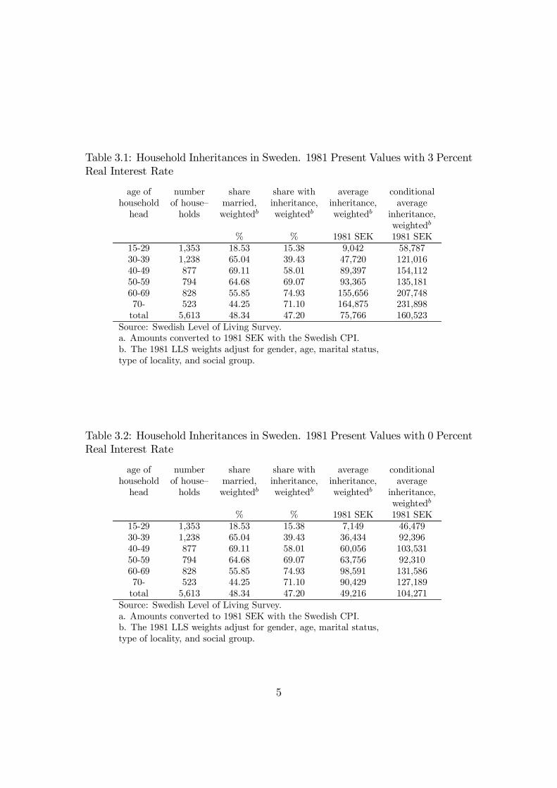
Table 3.1: Household Inheritances in Sweden. 1981 Present Values with 3 PercentReal Interest Rate

age of number share share with average conditionalhousehold of house– married, inheritance, inheritance, average

head holds weightedb weightedb weightedb inheritance,weightedb

% % 1981 SEK 1981 SEK15-29 1,353 18.53 15.38 9,042 58,78730-39 1,238 65.04 39.43 47,720 121,01640-49 877 69.11 58.01 89,397 154,11250-59 794 64.68 69.07 93,365 135,18160-69 828 55.85 74.93 155,656 207,74870- 523 44.25 71.10 164,875 231,898

total 5,613 48.34 47.20 75,766 160,523Source: Swedish Level of Living Survey.a. Amounts converted to 1981 SEK with the Swedish CPI.b. The 1981 LLS weights adjust for gender, age, marital status,type of locality, and social group.

Table 3.2: Household Inheritances in Sweden. 1981 Present Values with 0 PercentReal Interest Rate



% % 1981 SEK 1981 SEK15-29 1,353 18.53 15.38 7,149 46,47930-39 1,238 65.04 39.43 36,434 92,39640-49 877 69.11 58.01 60,056 103,53150-59 794 64.68 69.07 63,756 92,31060-69 828 55.85 74.93 98,591 131,58670- 523 44.25 71.10 90,429 127,189

total 5,613 48.34 47.20 49,216 104,271Source: Swedish Level of Living Survey.a. Amounts converted to 1981 SEK with the Swedish CPI.b. The 1981 LLS weights adjust for gender, age, marital status,type of locality, and social group.

5

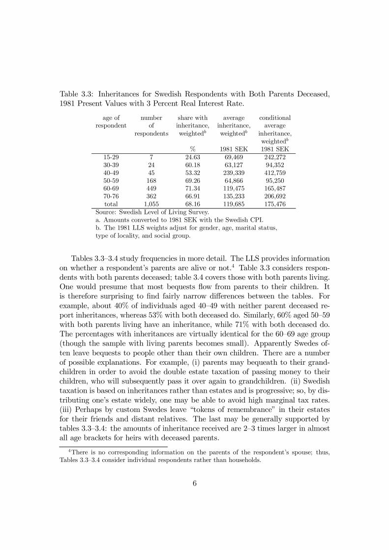
Table 3.3: Inheritances for Swedish Respondents with Both Parents Deceased,1981 Present Values with 3 Percent Real Interest Rate.

age of number share with average conditionalrespondent of inheritance, inheritance, average

respondents weightedb weightedb inheritance,weightedb

% 1981 SEK 1981 SEK15-29 7 24.63 69,469 242,27230-39 24 60.18 63,127 94,35240-49 45 53.32 239,339 412,75950-59 168 69.26 64,866 95,25060-69 449 71.34 119,475 165,48770-76 362 66.91 135,233 206,692total 1,055 68.16 119,685 175,476

Source: Swedish Level of Living Survey.a. Amounts converted to 1981 SEK with the Swedish CPI.b. The 1981 LLS weights adjust for gender, age, marital status,type of locality, and social group.

Tables 3.3–3.4 study frequencies in more detail. The LLS provides informationon whether a respondent’s parents are alive or not.4 Table 3.3 considers respon-dents with both parents deceased; table 3.4 covers those with both parents living.One would presume that most bequests ‡ow from parents to their children. Itis therefore surprising to …nd fairly narrow di¤erences between the tables. Forexample, about 40% of individuals aged 40–49 with neither parent deceased re-port inheritances, whereas 53% with both deceased do. Similarly, 60% aged 50–59with both parents living have an inheritance, while 71% with both deceased do.The percentages with inheritances are virtually identical for the 60–69 age group(though the sample with living parents becomes small). Apparently Swedes of-ten leave bequests to people other than their own children. There are a numberof possible explanations. For example, (i) parents may bequeath to their grand-children in order to avoid the double estate taxation of passing money to theirchildren, who will subsequently pass it over again to grandchildren. (ii) Swedishtaxation is based on inheritances rather than estates and is progressive; so, by dis-tributing one’s estate widely, one may be able to avoid high marginal tax rates.(iii) Perhaps by custom Swedes leave “tokens of remembrance” in their estatesfor their friends and distant relatives. The last may be generally supported bytables 3.3–3.4: the amounts of inheritance received are 2–3 times larger in almostall age brackets for heirs with deceased parents.

4There is no corresponding information on the parents of the respondent’s spouse; thus,Tables 3.3–3.4 consider individual respondents rather than households.

6

Table 3.4: Inheritances for Swedish Respondents with Both Parents Living, 1981Present Values with 3 Percent Real Interest Rate.


respondents weightedb weightedb inheritance,weightedb

% 1981 SEK 1981 SEK15-29 1,355 12.08 5,441 46,13930-39 1,029 25.50 26,767 101,61540-49 574 40.25 41,883 102,01850-59 276 59.86 45,171 81,09760-69 63 70.99 50,655 75,12770-76 7 75.63 60,251 83,401total 3,304 26.40 22,711 86,471

Source: Swedish Level of Living Survey.a. Amounts converted to 1981 SEK with the Swedish CPI.b. The 1981 LLS weights adjust for gender, age, marital status,type of locality, and social group.

(2) A second observation is that the inheritance amounts in Table 3.1 are nei-ther insigni…cant nor overwhelmingly large. Households aged 60 and above are themost likely to have completed their receipt of inheritances. The average amountreceived is 150,000–160,000 SEK for that category. As average household 1981earnings net of income taxes in the whole sample are 50,000 SEK, inheritancesseem to provide about 3 years earnings on average.5

Table 3.2 shows that interest accruing on amounts inherited is nontrivial, espe-cially for older households. In the literature, some authors advocate not countinginterest in assessing inheritances (see Modigliani (1988)). We take the view thata 3% interest rate is conservative and that only present values with the same timebase are comparable.

Tables 3.5–3.6 evaluate inheritance amounts in relative terms. Bringing wealthdata from Statistics Sweden, Table 3.5 shows that as a fraction of household networth, inheritances are very large. For the age group 60–69, for instance, averageinheritances (plus interest) are 60–65% as large as average measured householdnet worth. It is important to realize, however, that the reported wealth …gures areunderstated, as neither the Swedish nor the U.S. data below include capitalizedfuture pension or social security ‡ows. Furthermore, it is di¢cult to measure allcomponents of nonpension net worth accurately. The ratio of average net worthto average net–of–tax current earnings is 2.96 for the LLS, but it is 5.55 for thePSID. Although social spending may leave Swedes less dependent on their own

5Recall that amounts inherited themselves are net of taxes.

7

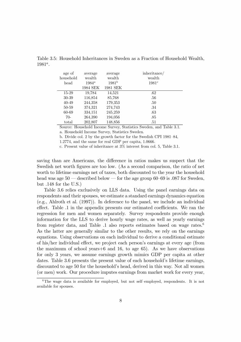
Table 3.5: Household Inheritances in Sweden as a Fraction of Household Wealth,1981a.

age of average average inheritance/household wealth wealth wealth

head 1984a 1981b 1981c

1984 SEK 1981 SEK15-29 19,784 14,521 .6230-39 116,854 85,768 .5640-49 244,358 179,353 .5050-59 374,321 274,743 .3460-69 334,151 245,259 .6370- 264,390 194,056 .85

total 202,807 148,856 .51Source: Household Income Survey, Statistics Sweden, and Table 3.1.a. Household Income Survey, Statistics Sweden.b. Divide col. 2 by the growth factor for the Swedish CPI 1981–84,1.2774, and the same for real GDP per capita, 1.0666.c. Present value of inheritance at 3% interest from col. 5, Table 3.1.

saving than are Americans, the di¤erence in ratios makes us suspect that theSwedish net worth …gures are too low. (As a second comparison, the ratio of networth to lifetime earnings net of taxes, both discounted to the year the householdhead was age 50 — described below — for the age group 60–69 is .087 for Sweden,but .148 for the U.S.)

Table 3.6 relies exclusively on LLS data. Using the panel earnings data onrespondents and their spouses, we estimate a standard earnings dynamics equation(e.g., Ahlroth et al. (1997)). In deference to the panel, we include an individuale¤ect. Table .1 in the appendix presents our estimated coe¢cients. We ran theregression for men and women separately. Survey respondents provide enoughinformation for the LLS to derive hourly wage rates, as well as yearly earningsfrom register data, and Table .1 also reports estimates based on wage rates.6

As the latter are generally similar to the other results, we rely on the earningsequations. Using observations on each individual to derive a conditional estimateof his/her individual e¤ect, we project each person’s earnings at every age (fromthe maximum of school years+6 and 16, to age 65). As we have observationsfor only 3 years, we assume earnings growth mimics GDP per capita at otherdates. Table 3.6 presents the present value of each household’s lifetime earnings,discounted to age 50 for the household’s head, derived in this way. Not all women(or men) work. Our procedure imputes earnings from market work for every year,

6The wage data is available for employed, but not self–employed, respondents. It is notavailable for spouses.

8

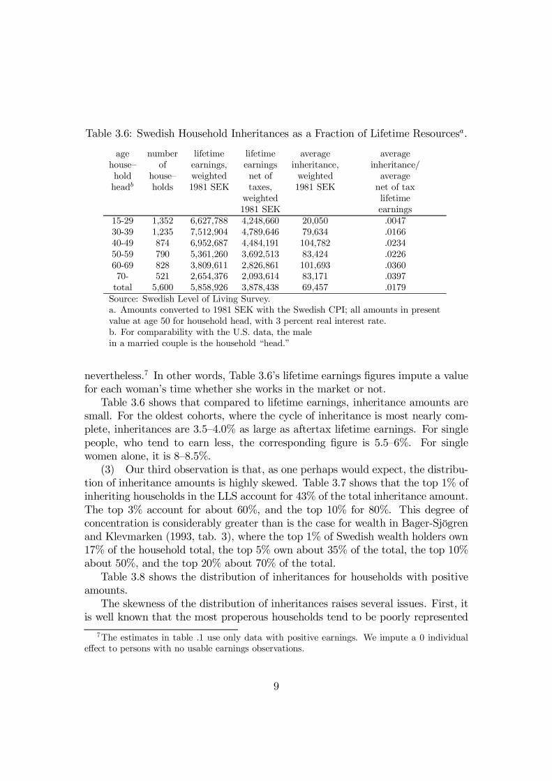
Table 3.6: Swedish Household Inheritances as a Fraction of Lifetime Resourcesa.

age number lifetime lifetime average averagehouse– of earnings, earnings inheritance, inheritance/hold house– weighted net of weighted averageheadb holds 1981 SEK taxes, 1981 SEK net of tax

weighted lifetime1981 SEK earnings

15-29 1,352 6,627,788 4,248,660 20,050 .004730-39 1,235 7,512,904 4,789,646 79,634 .016640-49 874 6,952,687 4,484,191 104,782 .023450-59 790 5,361,260 3,692,513 83,424 .022660-69 828 3,809,611 2,826,861 101,693 .036070- 521 2,654,376 2,093,614 83,171 .0397

total 5,600 5,858,926 3,878,438 69,457 .0179Source: Swedish Level of Living Survey.a. Amounts converted to 1981 SEK with the Swedish CPI; all amounts in presentvalue at age 50 for household head, with 3 percent real interest rate.b. For comparability with the U.S. data, the malein a married couple is the household “head.”

nevertheless.7 In other words, Table 3.6’s lifetime earnings …gures impute a valuefor each woman’s time whether she works in the market or not.

Table 3.6 shows that compared to lifetime earnings, inheritance amounts aresmall. For the oldest cohorts, where the cycle of inheritance is most nearly com-plete, inheritances are 3.5–4.0% as large as aftertax lifetime earnings. For singlepeople, who tend to earn less, the corresponding …gure is 5.5–6%. For singlewomen alone, it is 8–8.5%.

(3) Our third observation is that, as one perhaps would expect, the distribu-tion of inheritance amounts is highly skewed. Table 3.7 shows that the top 1% ofinheriting households in the LLS account for 43% of the total inheritance amount.The top 3% account for about 60%, and the top 10% for 80%. This degree ofconcentration is considerably greater than is the case for wealth in Bager-Sjögrenand Klevmarken (1993, tab. 3), where the top 1% of Swedish wealth holders own17% of the household total, the top 5% own about 35% of the total, the top 10%about 50%, and the top 20% about 70% of the total.

Table 3.8 shows the distribution of inheritances for households with positiveamounts.

The skewness of the distribution of inheritances raises several issues. First, itis well known that the most properous households tend to be poorly represented

7The estimates in table .1 use only data with positive earnings. We impute a 0 individuale¤ect to persons with no usable earnings observations.

9

Table 3.7: Distribution of Inheritances in Sweden for All Households (Inheritancesin 1981 Present Value with 3 Percent Real Interest Rate) a.

Bracket Smallest Average Fraction CumulativeInheritance Inheritance of Total Fraction ofin Bracket: in Bracket: Inheritances Inheritances1981 SEK 1981 SEK

top 1% 948,000 3,249,088 .43 .43top 1–2% 545,000 720,377 .10 .52top 2–3% 404,000 467,421 .06 .59top 3–5% 265,000 324,325 .09 .67top 5–10% 141,000 193,420 .13 .80top 10–15% 87,000 109,736 .07 .87top 15–20% 59,000 71,012 .05 .92top 20–25% 40,000 49,169 .03 .95top 25–50% 0 14,946 .05 1.00bottom 50% 0 0 .00 1.00Source: 1981 Swedish LLS.a. Sample size=5613.

Table 3.8: Distribution of Inheritances in Sweden for Households with PositiveAmounts (Inheritances in 1981 Present Value with 3 Percent Real Interest Rate)a.


top 1% 2,147,000 5,281,607 .33 .33top 1–2% 979,000 1,503,020 .09 .42top 2–3% 748,000 865,051 .05 .48top 3–5% 494,000 582,700 .07 .55top 5–10% 274,000 361,600 .11 .66top 10–15% 197,000 234,338 .07 .73top 15–20% 150,000 173,105 .05 .79top 20–25% 115,000 132,788 .04 .83top 25–50% 45,000 72,548 .11 .94bottom 50% 0 17,914 .06 1.00Source: 1981 Swedish LLS.a. Sample size=2847.

10

in data sets — they are few in number, and they tend to avoid participating insurveys. If, for example, top wealth holders are seriously underrepresented in theLLS, Table 3.7 warns that inheritance amounts might be severely understated.Second, Table 3.8 suggests that multiple motives may explain Swedish bequests.Inheritances in the bottom half of the distribution are quite small, perhaps re-sembling wedding gifts and graduation presents more than serious attempts toaugment heirs’ lifetime consumption possibilities. Amounts of money received bythe top 5%, on the other hand, correspond to many years of (average) earnings.A single behavioral model may not …t the widely varying sums.

Table 3.9 recomputes the distribution of inheritances in terms of present valueat age 50. An altruistic parent who cares about the lifetime resources of his childwould presumably think about his prospective bequest in such a way. The tableincludes only households aged 60–69, for whom the life cycle of inheritances maybe largely complete. As in Table 3.7, Table 3.9 encompasses all households inthe age category, including those with 0 inheritance. Table 3.10 computes thedistribution of aftertax lifetime labor earnings for the same sample. The contrastbetween Tables 3.9–3.10 is dramatic: the distribution of aftertax earnings is very,very equal compared with inheritances.8

(4) Most surveys fail to capture the richest segment of society (e.g., Daviesand Shorrocks (1996)), and Table 3.11 hints that the LLS, while perhaps doingbetter than most, may have the same problem. There is tax record data onearnings (and birth date) for all 6987 individuals in the original sample. 1374people did not respond to the mail survey (where, for instance, the questions oninheritances were). For di¤erent age groups, Table 3.11 orders male respondentsby their 1981 earnings, and presents survey response rates. Response rates arequite high and very level until we reach the top earners, at which point the ratestaper o¤ noticeably.9

8Several factors probably exaggerate the equality of earnings in Table 3.10 as follows. (i) Pre-dictions based on a random e¤ects model essentially average a person’s residual with the sampleaverage residual (which is 0), the person’s residual getting more weight if it is based on moreobservations. Yet, we have at most 3 observations per person. (ii) We predict out of sampleusing GDP per capita — doing so in the same way for all people. (iii) As noted above, weattribute market work in every year to all women, whereas in practice some do not work.

9It is di¢cult to draw conclusions from Table 3.11 other than the suspicion that the mostprosperous households are underrepresented. For example, the correlation coe¢cient betweencurrent earnings and inheritance amount for males aged 50–59 in the top 25% of the earningsdistribution for this group is only .033, and the corresponding correlation for males aged 60–69is .014.

11

Table 3.9: Distribution of Inheritances in Sweden for Households Ages 60–69(Inheritances in Present Value at Each Household’s 50th Birthday, with 3 PercentReal Interest Rate)a.


top 1% 1,392,155 3,665,698 .36 .36top 1–2% 669,685 1,008,029 .10 .46top 2–3% 476,723 597,508 .06 .52top 3–5% 352,733 423,397 .08 .60top 5–10% 172,962 242,253 .12 .72top 10–15% 112,358 144,160 .07 .79top 15–20% 82,594 99,851 .05 .84top 20–25% 63,328 72,889 .04 .88top 25–50% 21,188 39,952 .10 .97bottom 50% 0 5,022 .03 1.00Source: 1981 Swedish LLS.a. All households — not just those with positive inheritances. Sample size=828.

Table 3.10: Distribution of Aftertax Lifetime Earnings in Sweden for HouseholdsAges 60–69 (Lifetime Earnings in Present Value at Household’s 50th Birthday,with 3 Percent Real Interest Rate)a.

Lifetime Smallest Average Fraction CumulativeEarnings Lifetime Lifetime of Total FractionBracket Earnings Earnings Lifetime of Lifetime

in Bracket, in Bracket, Earnings Earnings1981 SEK 1981 SEK in Bracket

top 1% 5,818,675 6,557,654 .02 .02top 1–2% 5,543,012 5,694,660 .02 .04top 2–3% 5,178,652 5,671,955 .02 .06top 3–5% 4,958,921 5,286,509 .04 .10top 5–10% 4,496,676 4,798,096 .08 .18top 10–15% 4,249,619 4,414,444 .08 .26top 15–20% 4,011,466 4,200,272 .07 .34top 20–25% 3,822,017 3,951,873 .07 .41top 25–50% 2,833,012 3,381,054 .30 .71bottom 50% 0 1,623,915 .30 1.00Source: 1981 Swedish LLS.a. Sample size=828.

12

Table 3.11: Fractions of Swedish Males Responding to the LLS Survey, by CurrentEarnings and Agea.

Earnings Bracket Ages 40–49 Ages 50–59 Ages 60–69top 2.5% .62 .50 .54

top 2.5–5% .85 .81 .96top 5–10% 1.00 .80 .82top 10–20% .87 .82 .78top 20–30% .85 .76 .80top 30–40% .91 .78 .86top 40–50% .82 .77 .77top 50–60% .85 .86 .56top 60–70% .76 .88 .77top 70–80% .65 .70 .83top 80–90% .68 .67 .77

bottom decile .64 .81 .83Source: 1981 Swedish LLS.a. Recall that the LLS has register earnings for all householdsin the original sample, not just survey respondents.

4. Behavioral Models

The introduction notes that di¤erent theories of bequest behavior have very dif-ferent policy implications. Thus, it is potentially important to distinguish amongthe models. This section attempts to use regression analysis to do so empirically.

The following is a simple reduced form description of inheritance behavior:

Ii = f(Ypi ; Yi; Xi); (1)

where Ii is the 1981 present value of the cumulative inheritance of respondent i, Y piis the present value at age 50 of the lifetime aftertax earnings of the respondent’sparents, Yi is the present value at age 50 of the respondent’s lifetime aftertaxearnings, and Xi is a vector of other variables such as respondent age, sex, etc.The model is easiest to interpret for single people who are late enough in life tohave completed their cycle of inheritances. According to Barro and Becker, thepartial derivative of f(:) with respect to Y p should be positive: a parent with moreresources will want to share them with his descendants via a larger estate. If theparent knows his childrens’ earnings early enough in his life to adjust his plans,he will want to share more the lower the childrens’ earnings. That suggests anegative partial derivative for f(:) with respect to Y . (Alternatively, if the parentdoes not know his childrens’ earnings, or if he does not learn them long enoughbefore his retirement to act, the partial derivative of f(:) with respect to Y shouldbe 0.) According to the accidental–bequest model, the partial with respect to Y p

13

should again be positive, but the partial with respect to Y should be 0. In theexchange model, the partial with respect to Y p is positive, but the partial for Ymay be of either sign.

Unfortunately, if we limit ourselves to people who have never married, oursample becomes small. However, Laitner (1991)s analysis of assortative matingsuggests that the essence of the altruistic model may carry over for married peopleanalyzed as if they were single. The accidental and exchange models inherentlyallow us to treat heirs as individuals. We proceed using individuals as our unit ofanalysis.

To employ (1) in a regression, we append an error term:

Ii = f(Ypi ; Yi; Xi) + ´i + ²i: (2)

Think of the error’s …rst component, ´i, as registering the taste for altruism ofrespondent i’s parents, and think of the second part, ²i, as capturing, say, mea-surement error in Ii.

Table 4.1 reports very preliminary regressions. The sample is limited to re-spondents who are age 50 and above and both of whose parents are already de-creased.10 The sample size is 972. The dependent variable is the respondent’sinheritance, in present value at age 50. In the …rst two columns the independentvariables are: number of siblings; “were you poor when you grew up?” (1 yes, 0no); father graduated from high school or college (1 yes, 0 no); father belongedto high economic status occupational group (1 yes, 0 no); mother graduated fromhigh school or college; mother belonged to high occupational group; woman (1yes, 0 no); married (1 yes, 0 no); widow (1 yes, 0 no); age; age squared; presentvalue at age 50 of respondent’s aftertax lifetime earnings; and, a constant.

The probit and the Tobit in columns 1–2 display similar results. All threeof our theories predict a positive sign for the coe¢cient of Y p in (1). Table 4.1strongly supports that: the coe¢cient on growing up poor is negative and highlystatistically signi…cant; the father’s (and sometimes the mother’s) occupationalstatus has a signi…cant, positive coe¢cient. The altruistic model predicts a nega-tive coe¢cient for Y , and the accidental model predicts a zero coe¢cient. The co-e¢cient comes out negative in both the probit and Tobit, but it is not statisticallysigni…cant in either case. Respondents with more siblings are not signi…cantly lesslikely to receive an inheritance, but when they do receive one, it is likely to besmaller.

Taken literally, columns 1–2 support the exchange and accidental models, andthey reject the altruistic model. However, this is very preliminary work, and there

10Note that the LLS does not contain information about spouses’ parents. Table 4.1 refers toinheritances of respondents — not of the households of respondents.

14

Table 4.1: Swedish Data: Regression Models of Inheritance Behavior, Coe¢cients(absolute T–statistic).

Independent Probit: Tobit: Probit: Tobit:Variablea Inheritance>0 Inheritance Inheritance>0 Inheritance

Amount Amountnumber -.025 -11.15 -.020 -9.04siblings (1.62) (2.60) (1.24) (2.08)

poor when -.54 -130.62 -.52 -123.94growing up (5.97) (5.23) (5.73) (4.96)

father -.13 84.15 -.28 41.29h.s./college (.54) (1.47) (1.15) (.70)father high .38 67.41 .34 54.92occ. group (3.88) (2.66) (3.38) (2.14)

mother .25 -21.54 .16 -40.83h.s./college (.55) (.21) (.34) (.41)mother high .38 49.80 .37 45.66occ. group (2.39) (1.41) (2.32) (1.30)

woman .0060 19.97 -.029 10.82(.05) (.63) (.23) (.34)

married .19 -27.44 .19 -26.13(1.66) (.91) (1.70) (.87)

widow -.037 5.73 -.015 9.23(.25) (.14) (.10) (.23)

age .13 29.99 .14 34.34(1.03) (.94) (1.16) (1.07)

age -.0010 -.24 -.0012 -.27squared (1.09) (.95) (1.22) (1.09)lifetime -.000079 -.0040 -.00013 -.016earnings (1.08) (.22) (1.65) (.88)schooling .. .. .049 12.86

years (2.55) (2.81)constant -3.11 -893.98 -3.95 -1121.39

(.79) (.87) (.99) (1.09)observations 972 950 972 950log likelihood -556.72 -4807.59 -553.38 -4803.65pseudo R2 .084 .0078 .090 .0086

Source: LLS; both parents dead and respondent age 50 or over.a. Unless explicitly noted, all variables refer to respondent.

15

are a number of potential problems. One is errors in variables in the constructedrespondent lifetime earnings regressor, Y . Perhaps even more important, we have5 proxies for Y p rather than a direct measure. Existing work on intertemporalearnings relationships implies that our Y may be correlated with incompletelycaptured components of Y p. This could lead to an upward bias on the coe¢cientof Y .

Another possible problem is as follows. The Becker model suggests that analtruistic parent …rst transfers human capital to his children. The parent turns togifts and bequests of money only if he desires to make additional transfers afterhe provides enough human capital to reduce its marginal bene…t to its marginalcost. This suggests that Yi may be endogenous, say,

Yi = Y (í); (3)

where í is as in (2), and where @Y=@í > 0.11

The regressions of columns 3–4 of Table 4.1 attempt to eliminate the corre-lation between í and Yi by adding the respondent’s years of education as anindependent variable. The coe¢cient on the heir’s lifetime earnings is larger inabsolute magnitude than in columns 1–2. In the probit, it is signi…cantly negativeat the 10% level.

5. U.S. Data

Our U.S. data comes from the Panel Study of Income Dynamics (PSID). ThePSID consists of panel data on annual earnings from 1967 to the present, togetherwith measurements of household net worth in 1984, 89, and 94. The 1984 wealthmodule included questions on cumulative inheritances. Later surveys asked abouttransfer ‡ows after 1984, sometimes with modi…ed wording. For conformity withthe Swedish data, we restrict our attention to the wealth and inheritance …guresfor 1984.

Our 1984 sample starts with 6918 households. There are 3807 couples, of whichwe dropped 29 for missing birth dates; 1233 single males, of which we dropped210 for missing birth dates; and, 1878 single females, of which we dropped 2 formissing birth dates. The …nal sample is 6677.

The 1984 questions about inheritances are:(V10937) Now we’re interested in where people’s assets come from. Have you

(or anyone in your family living there) ever inherited any money or property?

11Although education is publicly funded to a higher degree in Sweden than, say, in the U.S.,parents undoubtedly provide subsidies to students in both places.

16

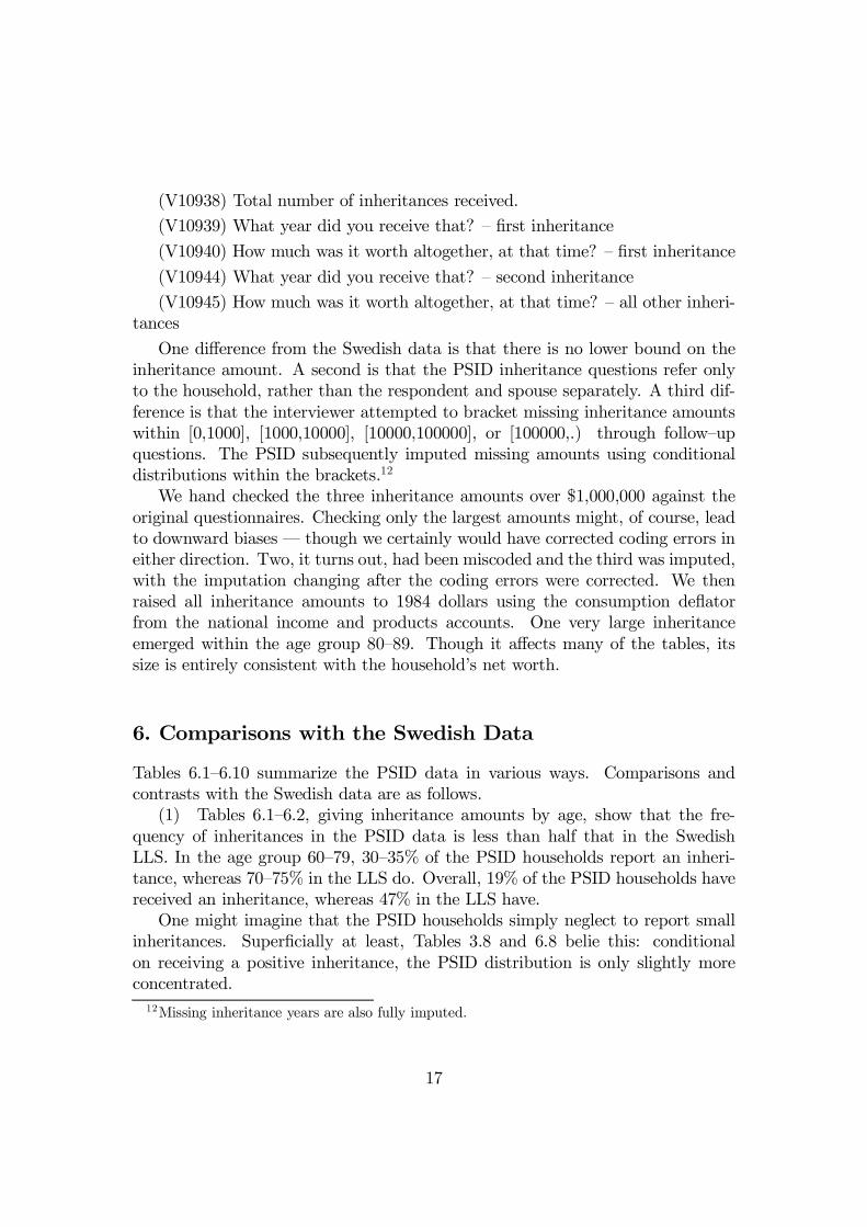
(V10938) Total number of inheritances received.

(V10939) What year did you receive that? – …rst inheritance

(V10940) How much was it worth altogether, at that time? – …rst inheritance

(V10944) What year did you receive that? – second inheritance

(V10945) How much was it worth altogether, at that time? – all other inheri-tances

One di¤erence from the Swedish data is that there is no lower bound on theinheritance amount. A second is that the PSID inheritance questions refer onlyto the household, rather than the respondent and spouse separately. A third dif-ference is that the interviewer attempted to bracket missing inheritance amountswithin [0,1000], [1000,10000], [10000,100000], or [100000,.) through follow–upquestions. The PSID subsequently imputed missing amounts using conditionaldistributions within the brackets.12

We hand checked the three inheritance amounts over $1,000,000 against theoriginal questionnaires. Checking only the largest amounts might, of course, leadto downward biases — though we certainly would have corrected coding errors ineither direction. Two, it turns out, had been miscoded and the third was imputed,with the imputation changing after the coding errors were corrected. We thenraised all inheritance amounts to 1984 dollars using the consumption de‡atorfrom the national income and products accounts. One very large inheritanceemerged within the age group 80–89. Though it a¤ects many of the tables, itssize is entirely consistent with the household’s net worth.

6. Comparisons with the Swedish Data

Tables 6.1–6.10 summarize the PSID data in various ways. Comparisons andcontrasts with the Swedish data are as follows.

(1) Tables 6.1–6.2, giving inheritance amounts by age, show that the fre-quency of inheritances in the PSID data is less than half that in the SwedishLLS. In the age group 60–79, 30–35% of the PSID households report an inheri-tance, whereas 70–75% in the LLS do. Overall, 19% of the PSID households havereceived an inheritance, whereas 47% in the LLS have.

One might imagine that the PSID households simply neglect to report smallinheritances. Super…cially at least, Tables 3.8 and 6.8 belie this: conditionalon receiving a positive inheritance, the PSID distribution is only slightly moreconcentrated.

12Missing inheritance years are also fully imputed.

17

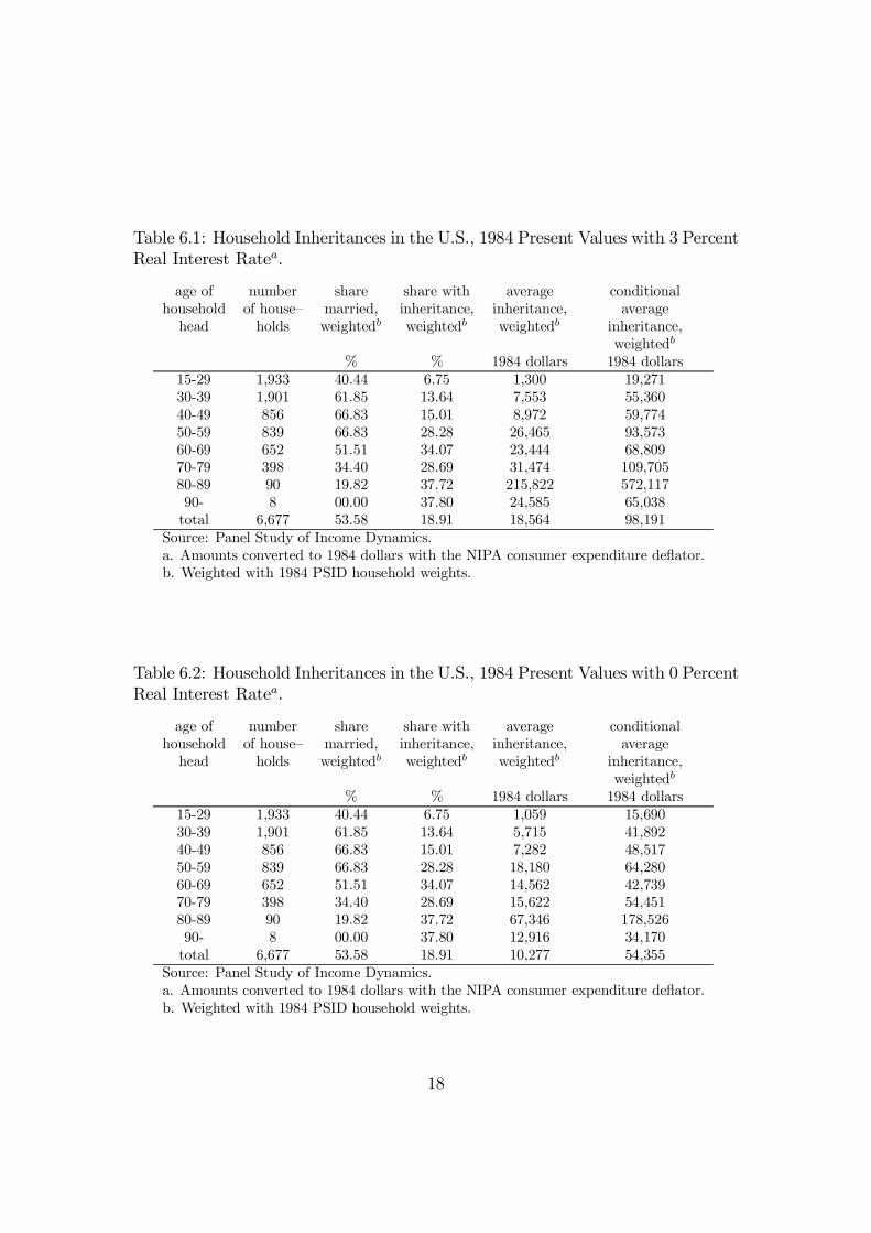
Table 6.1: Household Inheritances in the U.S., 1984 Present Values with 3 PercentReal Interest Ratea.



% % 1984 dollars 1984 dollars15-29 1,933 40.44 6.75 1,300 19,27130-39 1,901 61.85 13.64 7,553 55,36040-49 856 66.83 15.01 8,972 59,77450-59 839 66.83 28.28 26,465 93,57360-69 652 51.51 34.07 23,444 68,80970-79 398 34.40 28.69 31,474 109,70580-89 90 19.82 37.72 215,822 572,11790- 8 00.00 37.80 24,585 65,038

total 6,677 53.58 18.91 18,564 98,191Source: Panel Study of Income Dynamics.a. Amounts converted to 1984 dollars with the NIPA consumer expenditure de‡ator.b. Weighted with 1984 PSID household weights.

Table 6.2: Household Inheritances in the U.S., 1984 Present Values with 0 PercentReal Interest Ratea.



% % 1984 dollars 1984 dollars15-29 1,933 40.44 6.75 1,059 15,69030-39 1,901 61.85 13.64 5,715 41,89240-49 856 66.83 15.01 7,282 48,51750-59 839 66.83 28.28 18,180 64,28060-69 652 51.51 34.07 14,562 42,73970-79 398 34.40 28.69 15,622 54,45180-89 90 19.82 37.72 67,346 178,52690- 8 00.00 37.80 12,916 34,170

total 6,677 53.58 18.91 10,277 54,355Source: Panel Study of Income Dynamics.a. Amounts converted to 1984 dollars with the NIPA consumer expenditure de‡ator.b. Weighted with 1984 PSID household weights.

18

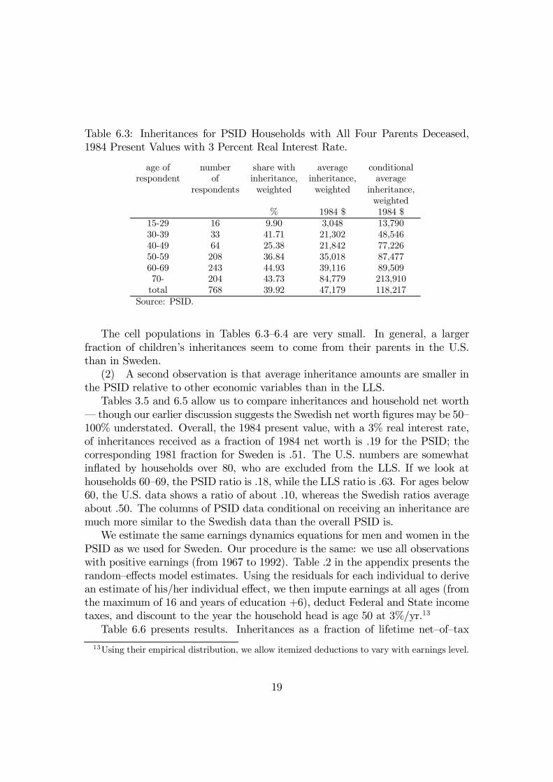
Table 6.3: Inheritances for PSID Households with All Four Parents Deceased,1984 Present Values with 3 Percent Real Interest Rate.


respondents weighted weighted inheritance,weighted

% 1984 $ 1984 $15-29 16 9.90 3,048 13,79030-39 33 41.71 21,302 48,54640-49 64 25.38 21,842 77,22650-59 208 36.84 35,018 87,47760-69 243 44.93 39,116 89,50970- 204 43.73 84,779 213,910

total 768 39.92 47,179 118,217Source: PSID.

The cell populations in Tables 6.3–6.4 are very small. In general, a largerfraction of children’s inheritances seem to come from their parents in the U.S.than in Sweden.

(2) A second observation is that average inheritance amounts are smaller inthe PSID relative to other economic variables than in the LLS.

Tables 3.5 and 6.5 allow us to compare inheritances and household net worth— though our earlier discussion suggests the Swedish net worth …gures may be 50–100% understated. Overall, the 1984 present value, with a 3% real interest rate,of inheritances received as a fraction of 1984 net worth is .19 for the PSID; thecorresponding 1981 fraction for Sweden is .51. The U.S. numbers are somewhatin‡ated by households over 80, who are excluded from the LLS. If we look athouseholds 60–69, the PSID ratio is .18, while the LLS ratio is .63. For ages below60, the U.S. data shows a ratio of about .10, whereas the Swedish ratios averageabout .50. The columns of PSID data conditional on receiving an inheritance aremuch more similar to the Swedish data than the overall PSID is.

We estimate the same earnings dynamics equations for men and women in thePSID as we used for Sweden. Our procedure is the same: we use all observationswith positive earnings (from 1967 to 1992). Table .2 in the appendix presents therandom–e¤ects model estimates. Using the residuals for each individual to derivean estimate of his/her individual e¤ect, we then impute earnings at all ages (fromthe maximum of 16 and years of education +6), deduct Federal and State incometaxes, and discount to the year the household head is age 50 at 3%/yr.13

Table 6.6 presents results. Inheritances as a fraction of lifetime net–of–tax

13Using their empirical distribution, we allow itemized deductions to vary with earnings level.

19

Table 6.4: Inheritances for PSID Households with All Four Parents Living, 1984Present Values with 3 Percent Real Interest Rate.


respondents weighted weighted inheritance,weighted

% 1984 $ 198415-29 1,0057 4.14 501 11,60530-39 736 8.54 4,177 45,79040-49 172 11.78 13,020 138,98650-59 31 20.90 4,436 25,60360-69 3 0 0 070- 1 100.00 55,996 41,703

total 2,000 6.78 3,018 44,515Source: PSID.

Table 6.5: U.S. Household Inheritances as a Fraction of Household Wealth in1984.

all conditional onhouseholds positive inheritance

age number average inheritance/ average inheritance/household of wealth wealth wealth wealth

head households 1984 1984a 1984 1984a

15-29 1,933 15,247 .09 29,843 .6530-39 1,901 69,481 .11 122,281 .4540-49 856 126,556 .07 147,984 .4050-59 839 215,710 .12 177,417 .5360-69 652 132,140 .18 191,659 .3670-79 398 96,410 .33 152,661 .7280-89 90 194,869 1.11 401,141 1.4390- 8 25,045 .98 46,727 1.39

total 6,677 100,021 .19 162,779 .60Source: Panel Study of Income Dynamics.a. 1984 present value of inheritance at 3% real interest rate.

20

Table 6.6: U.S. Household Inheritances as a Fraction of Lifetime Resourcesa.

age number lifetime lifetime average averagehouse– of earnings, earnings inheritance, inheritance/hold house– weighted net of weighted averageheadb holds 1984 $ taxes, 1984 $ net of tax

weighted lifetime1984 $ earnings

15-29 1,933 2,087,479 1,467,399 2,650 .001830-39 1,901 2,059,601 1,458,093 11,679 .008040-49 856 1,850,065 1,328,144 10,478 .007950-59 839 1,571,867 1,149,009 22,640 .019760-69 652 1,173,803 894,793 15,150 .016970-79 398 861,129 690,124 15,258 .022180-89 90 597,444 508,487 83,478 .164290- 8 278,829 261,312 6,430 .0246

total 6,677 1,709,820 1,233,212 13,678 .0111Source: PSID.a. Amounts converted to 1984 dollars with the NIPA consumer expenditurede‡ator; all amounts in present value at age 50 for household head,with 3 percent real interest rate.b. Following the PSID convention, the male in a married couple is the “head.”

earnings are 60% lower in the PSID than the LLS. The fraction is one–third lessfor the 60–69 age group. The overall (i.e., for all age groups) average inheritancein the PSID provides almost exactly one year’s current net–of–tax earnings; inSweden, the corresponding …gure is 1.5 years.

As stated, the sample sizes in Tables 6.3–6.4 are very small. Nevertheless,in contrast to the Swedish data, the conditional average inheritance amounts forhouseholds with and without deceased parents seem quite similar (i.e., considerthe …rst three age categories).

(3) The PSID data shows a distribution of inheritances more concentratedthan the distribution of net worth, which, in turn, is more concentrated than thedistribution of earnings. This is apparent for Tables 6.9–6.10, where we isolatethe age group 60–69. The comparisons resemble the Swedish data, though theU.S. distributions are more unequal.

(4) It is well–known that the PSID does not provide a good representationof very wealthy households. For example, Hurst, Luoh, and Sta¤ord [1996] arguethat the 1994 PSID accurately characterizes the U.S. distribution of wealth up toamounts of $1,000,000, but not over. That leaves the top 2–3% of wealth holders— who seem to control about 40% of U.S. net worth — poorly characterized.14

14The point is that the very rich may behave di¤erently from the rest of population. (We cannote that within the PSID sample, the raw correlation between wealth and inheritances received

21

Table 6.7: Distribution of Inheritances in the PSID for All Households (Inheri-tances in 1984 Present Value with 3 Percent Real Interest Rate)a.

Bracket Smallest Average Fraction CumulativeInheritance Inheritance of Total Fraction ofin Bracket: in Bracket: Inheritances Inheritances1984 dollars 1984 dollars

top 1% 287,639 1,059,954 .57 .57top 1–2% 173,603 215,089 .12 .69top 2–3% 115,062 148,145 .08 .77top 3–5% 64,079 87,694 .09 .86top 5–10% 19,260 38,337 .10 .96top 10–15% 5,293 11,372 .03 1.00top 15–20% 0 1,861 .01 1.00top 20–25% 0 0 .00 1.00top 25–50% 0 0 .00 1.00bottom 50% 0 0 .00 1.00Source: 1984 U.S. PSID.a. Sample size=6677.

Table 6.8: Distribution of Inheritances in the PSID for Households ReceivingPositive Amounts (Inheritances in 1984 Present Value with 3 Percent Real InterestRate)a.


top 1% 1,118,820 3,630,344 .37 .37top 1–2% 540,236 816,113 .08 .45top 2–3% 384,303 483,134 .05 .50top 3–5% 294,046 331,086 .07 .57top 5–10% 173,784 220,042 .11 .68top 10–15% 125,398 149,408 .08 .76top 15–20% 90,171 106,494 .05 .81top 20–25% 70,042 79,083 .04 .85top 25–50% 22,543 41,712 .11 .96bottom 50% 0 8,027 .04 1.00Source: 1984 U.S. PSID.a. Sample size=921.

22

Table 6.9: Distribution of Inheritances in the U.S. for Households Ages 60–69(Inheritances in Present Value at Each Household’s 50th Birthday, with 3 PercentReal Interest Rate)a.


top 1% 190,871 315,482 .21 .21top 1–2% 167,946 198,887 .13 .34top 2–3% 121,284 167,686 .11 .45top 3–5% 92,980 114,120 .15 .60top 5–10% 37,228 63,646 .21 .81top 10–15% 20,155 29,304 .10 .91top 15–20% 10,911 15,462 .05 .96top 20–25% 6,622 8,618 .03 .99top 25–50% 0 783 .01 1.00bottom 50% 0 0 .00 1.00Source: 1984 PSID.a. All households — not just those with positive inheritances. Sample size=652.

Table 6.10: Distribution of Aftertax Lifetime Earnings in the U.S. for HouseholdsAges 60–69 (Lifetime Earnings in Present Value at Household’s 50th Birthday,with 3 Percent Real Interest Rate)a.

Lifetime Smallest Average Fraction CumulativeEarnings Lifetime Lifetime of Total Fraction ofBracket Earnings Earnings Lifetime Lifetime

in Bracket, in Bracket, Earnings Earnings1984 $ 1984 $ in Bracket

top 1% 2,382,744 2,961,416 .03 .03top 1–2% 2,166,875 2,761,246 .03 .06top 2–3% 2,024,953 2,216,875 .02 .09top 3–5% 1,866,338 2,037,435 .04 .13top 5–10% 1,619,768 1,752,582 .10 .23top 10–15% 1,476,384 1,553,193 .09 .32top 15–20% 1,351,168 1,446,497 .08 .40top 20–25% 1,263,819 1,328,697 .07 .47top 25–50% 818,283 1,061,929 .30 .77bottom 50% 0 402,192 .23 1.00Source: PSID.a. Sample size=652.

23

7. Behavioral Model

Table 7.1 presents regression estimates of our behavioral model for the U.S. data.As in the Swedish case, we restrict the sample to people aged 50 and over, withboth parents deceased. The reported regressions refer to single people. Thesample for couples with all parents deceased is even smaller, we do not have thefather’s occupational group for wives, and results for couples are quite similar tothose in Table 7.1.

As in the Swedish data, number of siblings has a negative e¤ect on the prob-ability of receiving any inheritance and on the amount received. Being “poor”when growing up had a signi…cant, negative e¤ect in all of the Swedish regres-sions, but it is insigni…cant in Table 7.1 — as is growing up “rich.” The Americansample grew up during the Great Depression and World War II, and perhapsthe …nancial status of their parents during those years did not accurately predicttheir well–being later on. As in the Swedish data, in Table 7.1 high occupationalstatus/high education parents are generally more likely to leave a bequest, andthe bequest they leave is likely to be larger. However, education rather than oc-cupational group is more signi…cant in the U.S. data. As in the Swedish data,respondent education has a positive, highly signi…cant coe¢cient.

The coe¢cient on the respondent’s lifetime earnings is important in distin-guishing among theories. In the Swedish data, the coe¢cient was negative, thoughgenerally insigni…cant. In Table 7.1, the coe¢cient is negative in 3 of 4 columns— though statistically signi…cant at the 5% level in only one case. A negativecoe¢cient is consistent with the altruistic model.

The dummy variable for being a woman has a negative coe¢cient in bothTobits of Table 7.1. Evidence suggests that siblings are treated equally in theirparents estates. One possibility is, therefore, that our “woman” variable merelyserves to o¤set in our regressions the di¤erence between male and female lifetimeearnings. In Table 7.1 we divide the household inheritance of a widow by 2 — forcompatibility in per capita terms with people who never married. Nevertheless,a widow is more likely to have a positive inheritance. Somewhat surprisingly,widows are also likely to have larger inheritance amounts. Perhaps widows recordlegacies from their spouses.

is weak: within the age group 50–59, for the wealthiest 25% of couples the correlation is -.043;for the age group 60–69, the same is .069.)

24

Table 7.1: U.S. Data: Regression Models of Inheritance Behavior, Coe¢cients(absolute T–statistic).

Independent Probit: Tobit: Probit: Tobit:Variablea Inheritance>0 Inheritance Inheritance>0 Inheritance

Amount Amountnumber -.085 -11641.32 -.080 -9865.19siblings (3.044) (2.515) (2.754) (2.173)

poor when .130 11910.32 .217 21493.47growing up (.660) (.369) (1.078) (.682)rich when .291 15449.02 .208 5640.72growing up (1.099) (.365) (.757) (.136)

father -.0089 64253.44 -.060 56576.88h.s./college (.037) (1.768) (.240) (1.593)father high .131 43814.76 -.051 24565.29occ. group (.573) (1.191) (.215) (.687)

mother .699 46907.86 .422 -2067.90h.s./college (3.560) (1.509) (2.000) (.065)

woman .185 -41087.27 -.018 -73953.57(.766) (1.104) (.071) (1.994)

widow .398 57167.31 .452 61132.21(2.225) (1.903) (2.424) (2.044)

age .177 37075.4 .229 41926.93(1.367) (1.663) (1.709) (1.901)

age -.0013 -285.75 -.0017 -319.47squared (1.329) (1.680) (1.650) (1.898)lifetime -1.27e-07 .00714 -6.21e-07 -.061earnings (.489) (.183) (2.137) (1.471)schooling .. .. .132 19167.7

years (4.223) (4.102)constant -6.742 -1308876 -9.676 -1638079

(1.596) (1.812) (2.184) (2.273)observations 310 290 310 290

Â2(11) 38.95 26.87 58.17 45.59log likelihood -167.281 -1008.896 -157.671 -999.535pseudo R2 .104 .0141 .156 .0223

Source: PSID; single people, aged 50 and over, with both parents dead.a. Unless explicitly noted, all variables refer to respondent.

25

8. Conclusion

Our data suggests that inheritances are far more prevalent in Sweden than in theU.S. The average amount inherited, relative to earnings, is also larger in Sweden,though not in proportion to incidence — as the American inheritances tend to besomewhat larger.

It seems likely that the U.S. data understates total inheritance amounts be-cause our sample does not provide good coverage of the wealthiest households.There is less evidence on the quality of the Swedish data in this regard.

Our behavioral analysis is still at an early stage. Very preliminary evidenceshows negative regression coe¢cients on respondent lifetime earnings, as wouldbe consistent with altruistic models. However, the statistical signi…cance of thenegative coe¢cients is marginal at best — perhaps pointing to the accidentalmodel (which predicts that the coe¢cients will be 0).

26

A. Appendix

27

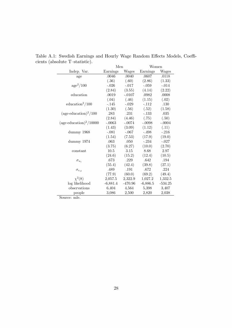
Table A.1: Swedish Earnings and Hourly Wage Random E¤ects Models, Coe¢-cients (absolute T–statistic).

Men WomenIndep. Var. Earnings Wages Earnings Wages

age .0046 .0040 .0607 .0118(.36) (.60) (2.86) (1.33)

age2/100 -.026 -.017 -.059 -.014(2.84) (3.55) (4.14) (2.22)

education .0019 -.0107 .0982 .0008(.04) (.46) (1.15) (.02)

education2/100 -.145 -.029 -.112 .130(1.30) (.56) (.52) (1.58)

(age¢education)2/100 .283 .231 -.133 .035(2.84) (4.46) (.75) (.50)

(age¢education)2/10000 -.0063 -.0074 -.0098 -.0004(1.43) (3.09) (1.12) (.11)

dummy 1968 -.081 -.067 -.498 -.216(1.54) (7.53) (17.9) (19.0)

dummy 1974 .063 .050 -.234 -.027(3.75) (6.27) (10.0) (2.70)

constant 10.5 3.15 8.68 2.97(24.6) (15.2) (12.4) (10.5)

¾ui.673 .229 .642 .194

(55.4) (42.4) (39.8) (27.1)¾eit .489 .191 .672 .224

(77.9) (60.0) (69.2) (49.4)Â2(8) 2,057.5 2,322.9 1,027.2 1,332.5

log likelihood -6,881.4 -470.96 -6,886.5 -534.25observations 6,404 4,564 5,398 3,407

people 3,086 2,500 2,820 2,038Source: mle.

28

Table A.2: PSID Earnings and Hourly Wage Random E¤ects Models, Coe¢cients(absolute T–statistic).

Men WomenIndep. Var. Earnings Wages Earnings Wages

age .084 .013 .178 -.013(10.665) (2.208) (11.410) (1.401)

age2/100 -.126 -.036 -.157 -.0042(24.182) (9.020) (15.824) (.734)

education -.053 -.094 .446 -.156(1.602) (3.755) (6.782) (4.252)

education2/100 .323 .401 -.603 .826(3.364) (5.632) (3.294) (8.499)

(age¢education)2/100 .259 .331 -.645 .312(4.672) (7.905) (5.533) (4.626)

(age¢education)2/10000 -.0035 -.011 .029 -.014(1.422) (5.900) (5.476) (4.404)

dummies 1967–91constant 7.468 1.426 2.034 1.648

(25.466) (6.472) (3.553) (5.088)¾ui

.630 .461 .957 .452(87.077) (89.092) (89.458) (87.642)

¾eit .538 .408 .779 .464(344.819) (345.526) (321.249) (322.197)

Â2(30) 46,557.18 50,803.03 34,808.34 34,067.79log likelihood -58,317.446 -40,245.411 -74,273.411 -43,299.450observations 64,523 64,496 57,480 57,453

Source: mle.

29

References

S. Ahlroth, A. Björklund, and A. Forslund. The output of the Swedish educationsector. Review of Income and Wealth, 43(1):89–104, March 1997.

J. G. Altonji, F. Hayashi, and L. J. Kotliko¤. Is the extended family altruisticallylinked? Direct tests using micro data. American Economic Review, 82(5):1177–1198, December 1992.

A. Auerbach and L. Kotliko¤. Dynamic Fiscal Policy. Cambridge UniversityPress, Cambridge, U.K., 1987.

L. Bager-Sjögren and A. Klevmarken. The distribution of wealth in Sweden.Research on Economic Inequality, 4, 1993.

R. J. Barro. Are government bonds net wealth? Journal of Political Economy,82(6):1095–1117, December 1974.

G. S. Becker. A theory of social interactions. Journal of Political Economy, 82(6):1063–1093, December 1974.

G. S. Becker and N. Tomes. An equilibrium theory of the distribution of incomeand intergenerational mobility. Journal of Political Economy, 87(6):1153–1189,December 1979.

B. D. Bernheim, A. Shleifer, and L. H. Summers. The strategic bequest motive.Journal of Political Economy, 93(6):1045–1076, December 1985.

A. Björklund and M. Jäntti. Intergenerational income mobility in Sweden com-pared to the United States. American Economic Review, 87(5):1009–1018, De-cember 1997.

C. Carroll and L. Summers. Consumption growth parallels income growth: Somenew evidence. In B. Bernheim and J. Shoven, editors, National Saving andEconomic Performance. University of Chicago Press, Chicago, 1994.

C. Chamley. Optimal taxation of capital income in general equilibrium within…nite lives. Econometrica, 54(3):607–622, June 1986.

J. B. Davies. Uncertain lifetime, consumption, and dissaving in retirement. Jour-nal of Political Economy, 89(3):561–577, June 1981.

30

J. B. Davies and A. Shorrocks. The distribution of wealth and its evolution. InA. Atkinson and F. Bourguignon, editors, Handbook of Income Distribution.1996. Forthcoming.

A. Drazen. Government debt, human capital, and bequests in a life–cycle model.Journal of Political Economy, 86(3):505–516, June 1978.

B. Friedman and M. Warshawsky. The cost of annuities: Implications for sav-ing behavior and bequests. Quarterly Journal of Economics, 105(1):135–154,February 1990.

L. J. Kotliko¤ and L. H. Summers. The role of intergenerational transfers inaggregate capital accumulation. Journal of Political Economy, 89(4):706–732,August 1981.

J. Laitner. Modeling marital connections along family lines. Journal of PoliticalEconomy, 99(6):1123–1141, December 1991.

J. Laitner. Random earnings di¤erences, lifetime liquidity constraints, and altru-istic intergenerational transfers. Journal of Economic Theory, 58(2):135–170,December 1992.

J. Laitner. Intergenerational and interhousehold economic links. In M. R. Rosen-zweig and O. Stark, editors, Handbook of Population and Family Economics,volume 1A, chapter 5, pages 189–238. North-Holland, Amsterdam, 1997.

J. Laitner and F. T. Juster. New evidence on altruism: A study of TIAA-CREFretirees. American Economic Review, 86(4):893–908, September 1996.

R. Mariger. Consumption Behavior and the E¤ects of Government Fiscal Policies.Harvard University Press, Cambridge, MA, 1986.

F. Modigliani. Life cycle, individual thrift, and the wealth of nations. AmericanEconomic Review, 76(3):672–690, June 1986.

F. Modigliani. The role of intergenerational transfers and life cycle saving in theaccumulation of wealth. Journal of Economic Perspectives, 2(2):15–40, Spring1988.

G. R. Solon. Intergenerational income mobility in the United States. AmericanEconomic Review, 82(3):393–408, June 1992.

N. Tomes. The family, inheritance, and the intergenerational transmission ofinequality. Journal of Political Economy, 89(5):928–958, October 1981.

31

equality of opportunity and inheritance: a comparison …uueconomics.se/henryo/describe.pdf ·...

Documents