ENVISAT RA-2 USO ANOMALY: IMPACT AND CORRECTION

Remko Scharroo1, Yannice Faugere2, Monica Roca3, Pierre Femenias4, Annalisa Martini5, and John Lillibridge6

1Altimetrics LLC, Cornish, New Hampshire, USA2CLS, Ramonville-St. Agne, France

3IsardSat, Barcelona, Catalunya4ESA/ESRIN, Frascati, Italy

5Serco, Frascati, Italy6NOAA Laboratory for Satellite Altimetry, Silver Spring, Maryland, USA

ABSTRACT

Starting in February 2006, the ranges measured by theEnvisat RA-2 altimeter have been biased significantly forlong periods of time. The range bias is characterised bya relatively constant offset of about 5.6 meters, and anadditional 1-cpr non-harmonic variation around the orbitwith an amplitude of about 10-20 cm.

The bias is caused by an anomalous operation of the Ul-tra Stable Oscillator (USO). Its frequency suddenly be-came biased by approximately 7 ppm plus a small varia-tion around the orbit. This paper discusses how the USObias can be modelled and corrected for. Also some spec-ulations are made as to the cause of the anomaly.

Key words: Envisat, RA-2, oscillator, calibration.

1. BACKGROUND

The first prolonged period that the Envisat altimeter suf-fered a bias of more than 5 meters was between 1 and 9February 2006 (Cycle 44 pass 856 until Cycle 45 pass 75)and then returned to a nearly nominal state. The secondperiod started on 13 March 2006 (Cycle 45 pass 990) andlasted until 28 February 2007 (Cycle 56 pass 54). A sim-ilar bias occurred between 27 and 29 September 2004.

The bias has both been blamed on the Ultra Stable Oscil-lator (USO) that provides the frequency standard for thealtimeter, and on the clock of the Instrument Control Unit(ICU) that provides the time tags to the altimeter data.From the observation that the bias has been introducedand has disappeared at least three times, it is extremelyunlikely that both USO and ICU clock are affected. Thechance that both sub-systems started to function abnor-mally and returned to nominal operation simultaneouslyseems infinitesimally small.

In the following it is therefore assumed that either theUSO or the ICU clock ceased nominal operation. Fromthis it can be demonstrated that it cannot be the ICUclock that is affected, leaving the USO as the culprit.

There are various indications that it is indeed the USOthat should be blamed for the altimeter range bias and itsvariation. The implications of a USO and ICU clock biasare different.

• In both cases a drift between the USO and ICU counterwill be noticeable in the USO, ICU, UTC triplets pro-vided in the Instrument Source Packet (ISP) headersand during the Kiruna time correlation [1].

• A USO frequency bias produces a scale bias in therange. If a USO bias exists, the range bias will be afunction of range itself. At the same time all time in-tervals related to the USO, like the pulse repetition in-terval (PRI, nominally 557 µs), will be scaled by thesame factor [2].

• A bias in the ICU clock results in a timing bias. Thisproduces an error in the sea surface heights propor-tional to the range rate. Hence the range bias will onlybe apparent, not real.

2. OBSERVED BIAS

The range bias can be determined by differencing sealevel anomalies (SLA) along collinear tracks. Fig. 1shows the SLA differences between Cycles 46 (affectedby the USO bias) and Cycle 45 (not affected). An aver-age bias of about 5.6 meters stands out. At the same timethe bias varies as a function of latitude and also differs be-tween ascending tracks (Fig. 1, left panel) and descendingtracks (right panel). On the other hand, the bias appearsgeographically correlated, i.e, it is consistent from oneascending pass to the next and from one descending passto the next. Note that in the right panel the latitude rangeis reversed so that the left and right panels are consecutivein time.

The black curves in Fig. 1 indicate the range biasthat would result from a constant 88 fs (femtoseconds,10−15s) error in the USO period. Since a USO biasproduces a scale bias to the range and the range varieswith latitude, the range bias varies with latitude as well.The comparison between the observed range bias and the

_____________________________________________________

Proc. ‘Envisat Symposium 2007’, Montreux, Switzerland 23–27 April 2007 (ESA SP-636, July 2007)

5.0

5.2

5.4

5.6

5.8

6.0

6.2

6.4∆S

LA (

m)

−60 −30 0 30 60

Latitude (deg)

5.0

5.2

5.4

5.6

5.8

6.0

6.2

6.4

∆SLA

(m

)

−60−3003060

Latitude (deg)

Figure 1. Observed sea level anomaly differences between Cycle 46 and Cycle 45, passes 76 to 568. Left panel: ascendingpasses; right panel: descending passes.

black curve makes it evident that the apparent USO biasis not constant but varies around the orbit.

The USO clock period is determined by differencing theICU clock at two instances and dividing the time intervalby the number of USO counts passed during that interval.In the standard processing this interval is 86400 s, ob-scuring any around-the-orbit variation of the USO period.Fig. 2 shows the USO period determined over intervals ofonly 100 s. The USO period varies around the orbit, as-suming that the ICU clock is functioning correctly.

Finally, we also observe a lengthening of the PRI. The“1-Hz” time interval of 2000 PRI, or 1.114000 seconds,has increased to 1.114007 seconds, adding 7 ppm.

3. HYPOTHESES

3.1. USO is functioning correctly

If the USO is still functioning correctly and in fact pro-duces a stable counter with a nominal beat period of12500000 fs, then the ICU clock must be defective. Theapparent USO periods observed and reported in [3], arecurrently about 88 fs longer than nominal, irrespective ofthe time interval over which they were computed. To pro-duce such a bias in the USO period, the ICU clock mustbe slow by a fraction of 7 ppm. This would lead to a clockoffset of 0.6 seconds every day. This is simply impossi-ble. Such an error would have been observed as soon asit accrues to more than a 1 ms, which takes only 140 s. Itwould sound serious alarms at the ICU/UTC time corre-lation. However, no significant changes in the ICU periodare observed [3].

An ICU clock bias of 1 ms leads to a maximum of 25 mmerror in the retrieved sea level as it is scaled by the rangerate which has a maximum of 25 m/s. Such errors caneasily be identified in crossover differences. However,

since the range rate is 0 m/s just north of the equator, thelocal error in sea level would be zero, independent of theICU clock bias. Fig. 1, however, shows that at the equatorthe error is significant, both in ascending and descendingtracks, even when a mean bias of 5.6 meters is subtracted.In other words, the apparent range bias is not proportionalto the range rate, as also shown in Fig. 3. This makes theexistence of an ICU clock bias highly unlikely.

Another case against the hypothesis of an ICU clock erroris that the ICU period is automatically calibrated againstUTC during every Kiruna overpass. Therefore the ICUperiod, on average will be correct even when otherwisenot being stable. Since we have postulated that the USOis functioning correctly, we should therefore see no meandrift between the USO and ICU clocks, which contradictsthe observations in [3].

3.2. ICU is functioning correctly

If the ICU is still functioning correctly, then the USO pe-riod must be varying to produce a range bias as shown inFig. 1. Since an error in the USO period implies a scaleerror in the range, it is relatively simple to solve the errorin the USO period from the range error, simply by divid-ing the observed range bias by the range and multiply-ing by the nominal USO period of 12500 ps. The resultis shown in Fig. 4. The result looks strikingly similar toFig. 2. The peak-to-peak variation from 86 to 91 fs agreesbetween the Figures, as does the steep upward slope andthe shallower downward slope. The only difference beingthat Fig. 2 implies a maximum at around 50◦S, whereasFig. 4 suggests that the maximum is around 43◦S.

The hypothesis that the USO is biased in a way as re-ported in [3] is therefore supported by the observed rangeerrors. Some further analysis of the observed USO pe-riod and the observed range bias is needed, particularlyto match the observed maxima in the curves of Fig. 2and Fig. 4. Furthermore, the variation of the USO pe-

5.3

5.4

5.5

5.6

5.7

5.8

∆ran

ge (

m)

00 01 02 03 04 05 06 07 08 09 10 11 12 13 14 15 16 17 18 19 20 21 22 23 00

Hours of 14 March 2006

82

84

86

88

90

∆US

O p

erio

d (f

s)

Figure 2. USO clock period evaluated over intervals of 100 s.

5.0

5.2

5.4

5.6

5.8

6.0

6.2

6.4

∆SLA

(m

)

−30 −25 −20 −15 −10 −5 0 5 10 15

Range rate (m/s)

5.0

5.2

5.4

5.6

5.8

6.0

6.2

6.4

∆SLA

(m

)

−15 −10 −5 0 5 10 15 20 25 30

Range rate (m/s)

Figure 3. Apparent range bias from Fig. 1 plotted against range rate. The absence of a clear relation between range biasand range rate makes it unlikely that the ICU clock is biased.

80

82

84

86

88

90

92

94

96

US

O p

erio

d bi

as (

fs)

−60 −30 0 30 60

Latitude (deg)

80

82

84

86

88

90

92

94

96U

SO

per

iod

bias

(fs

)

−60−3003060

Latitude (deg)

Figure 4. USO period bias derived from the apparent range biases shown in Fig. 1.

riod needs to be analysed: is it consistent from revolu-tion to revolution? Can it be modelled (and hence pre-dicted)? Can it be corrected for in addition to the back-ground drift?

The increase of the “1-Hz” time step by 7 ppm is alsoconsistent with an increase in the USO period by the samefraction. The two are related through the PRI. A changein the ICU period would not affect the PRI, nor wouldit even contribute to an apparent lengthening of the “1-Hz” time step (in UTC seconds) since the ICU period iscalibrated nearly every orbital revolution.

4. CONCLUSIONS SO FAR

The range bias of about 5.6 meter and its around-the-orbitvariation observed for long periods since February 2006is clearly not related to ICU clock errors. First, a clock er-ror would result in a range bias proportional to the rangerate (which it is not). Second, the ICU clock error wouldbe observed during the ICU/UTC time correlation (whichis not the case). Third, the observed increase in the “1-Hz” time step by 7 ppm can not be explained by an ICUclock error.

A bias in the USO period of about 88 fs is observedby comparing the USO counter against the ICU clock,and is confirmed by dividing the observed range bias bythe range and multiplying by the nominal USO period of12500 ps. In other words, both USO period and altimeterrange are scaled by about 7 ppm. Also an around-the-orbit variation of the USO period is apparent from bothmethods, and the observed amplitudes and phase agree.

In the rest of the paper, we will present a model that canbe created with only one month of data, has predictive ca-pabilities, is simple to implement, and models the short-term variation of the USO period to better than 0.016 fs (1mm in range). This model was eventually implementedin the Level 0 processing.

5. OBSERVATIONS OF THE USO PERIOD VARI-ATIONS

Input to the modelling exercise discussed in this paper aretwo sets of estimates of the variation of the USO period,determined by comparing the USO counter against theICU clock counter, which in turn is correlated to UTC.The data sets differ in the interval over which the twocounters are compared.

1. USO periods determined over intervals of 100 seconds,from 14 March to 6 May 2006. During periods whenthe USO returned to nominal operation (2-6 April) andperiods with large trends in the USO period were ex-cluded. Remaining were relative orbits 10-51, 57-283and 420-501 of Cycle 46; and relative orbits 1-289 ofCycle 47.

84

85

86

87

88

89

90

91

92

∆US

O p

erio

d (f

s)

0 1000 2000 3000 4000 5000 6000

Cycle 47, Orbit 288Cycle 46, Orbit 10 5.4

5.5

5.6

5.7

5.8

∆ran

ge (

m)

0 1000 2000 3000 4000 5000 6000

Time along orbit (s)

84

85

86

87

88

89

90

91

92

∆US

O p

erio

d (f

s)

72

73

74

75

76

77

78

79

80

∆US

O p

erio

d (f

s)

Cycle 46, Orbit 372Cycle 46, Orbit 419

Figure 5. Estimated USO period in excess of the nominal12500 ps. Determined with 100 second intervals. Hori-zontal axis is time since Southern culmination point (startof ascending pass). Top: Red dots are for Cycle 46, orbit10. Blue dots are for Cycle 47, orbit 288. Curves have thesame shape, but shifted left and up. Bottom: Red dots arefor Cycle 46, orbit 419 (left ordinate). Blue dots are forCycle 46, orbit 372 (right ordinate). Curves have the dif-ferent amplitudes, more or less proportional to the meanOSU bias.

2. USO periods determined over intervals of 25 seconds,from 27 March to 2 May 2006. Data between 2 and 6April was excluded when the USO shortly returned tonormal operations.

Because of the relatively short time intervals and the in-herently coarse resolution of the ICU clock, the USO pe-riod estimates are digitised with a step size of approxi-mately 0.2 fs, as shown in Fig. 5. The top of this Figureclearly illustrates that the short-term variation of the USOperiod is consistent between orbit 10 (14 March) and or-bit 288 (6 May), except for a shift towards the left andup. The horizontal shift by about 400 seconds is compat-ible with the procession of the eclipse entry Southwardby the same amount. It makes therefore sense to modelthe short-term variation of the USO period as a functionof time since entry of the eclipse. The vertical shift byabout 1 fs is “natural” long-term variation of the USOperiod.

During some days, particularly after instrument switch-on, the mean USO bias can be significantly less than the88 fs. The bottom half of Fig. 5 shows that during orbit372 of Cycle 46 the USO period is biased by only 76 fs.At the same time the around-the-orbit variation has alsodecreased in amplitude. This suggests that the 1-cpr vari-

0

200

400

600

800

1000E

clip

se e

ntry

tim

e (s

)

01 02 03 04 05 06 07 08 09 10 11 12

Month of Year

TabulatedFunction

Figure 6. Variation of the eclipse entry time during a year.Times are relative to the start of the ascending pass. Thered curve is based on tabular data for 2006 provided bythe Sciamachy project. The overlapping blue curve is aFourier series approximation used in this paper to modelthe USO period variation.

ation is proportional to the mean bias.

6. MODELLING THE USO PERIOD VARIA-TIONS

As shown in the previous section, the short-term variationis in phase with the time of the entry of the eclipse. Thetimes that Envisat enters and exits the eclipse are avail-able from the Sciamachy project, but are also easily mod-elled. Fig. 6 shows the tabulated entry times (with respectto the start of the ascending pass) as well as the resultsfrom a simple Fourier series function that fits the tabu-lated values to 4.6 seconds rms.

The model for the eclipse entry times can now be used tobring the solutions for the USO period along different or-bits in phase. What remains is a variable offset betweenthe different orbits that needs to be taken into accountwhen developing a model for the short-term variation ofthe USO period. Since this variation is clearly periodic,the variation is best approximated with a Fourier series.An even number (2n) of parameters (c1,s1, ...,cn,sn) isestimated to model the variation up to n cycles per rev-olution, while an additional m parameters (∆P j) are es-timated to capture the mean USO period offset for eachof the m orbits selected. With t being time since eclipseentry, the USO period offset (∆P) becomes

∆P(t) = ∆P j[1+∑(ci cos(iωt)+ si sin(iωt))] (1)

The number n should be small enough not to introduceany artifacts (for example resulting from the digitisationof the data) but large enough to model the variation tobetter than 1 mm in range. It was found that n = 10satisfies these criteria. Using that value, or any numberlarger than that, revealed that there was less than 0.015 fs(1 mm of equivalent range) accumulative power for any

−1.0−0.8−0.6−0.4−0.2

0.00.20.40.60.81.0

∆US

O p

erio

d (f

s)

0 1000 2000 3000 4000 5000

Time since eclipse entry (s)

−60

−40

−20

0

20

40

60

∆ran

ge (

mm

)

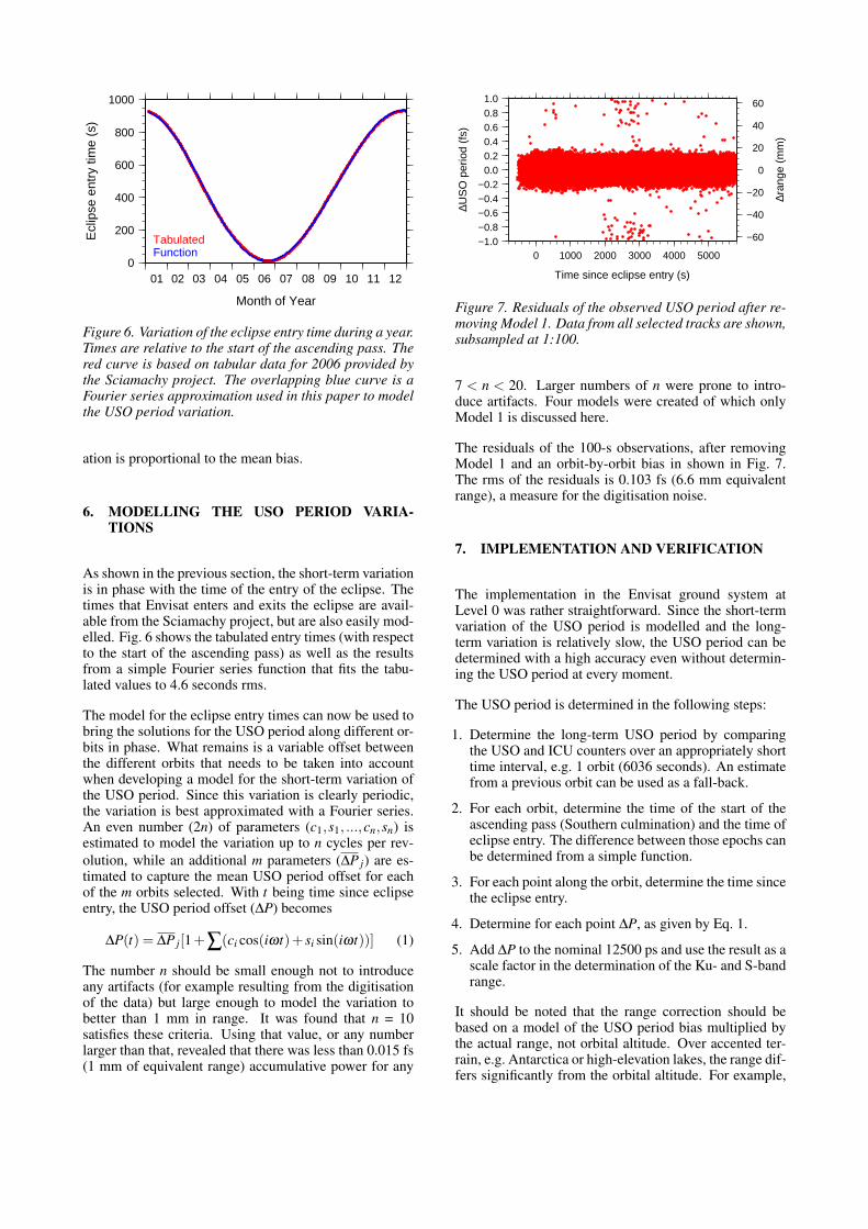
Figure 7. Residuals of the observed USO period after re-moving Model 1. Data from all selected tracks are shown,subsampled at 1:100.

7 < n < 20. Larger numbers of n were prone to intro-duce artifacts. Four models were created of which onlyModel 1 is discussed here.

The residuals of the 100-s observations, after removingModel 1 and an orbit-by-orbit bias in shown in Fig. 7.The rms of the residuals is 0.103 fs (6.6 mm equivalentrange), a measure for the digitisation noise.

7. IMPLEMENTATION AND VERIFICATION

The implementation in the Envisat ground system atLevel 0 was rather straightforward. Since the short-termvariation of the USO period is modelled and the long-term variation is relatively slow, the USO period can bedetermined with a high accuracy even without determin-ing the USO period at every moment.

The USO period is determined in the following steps:

1. Determine the long-term USO period by comparingthe USO and ICU counters over an appropriately shorttime interval, e.g. 1 orbit (6036 seconds). An estimatefrom a previous orbit can be used as a fall-back.

2. For each orbit, determine the time of the start of theascending pass (Southern culmination) and the time ofeclipse entry. The difference between those epochs canbe determined from a simple function.

3. For each point along the orbit, determine the time sincethe eclipse entry.

4. Determine for each point ∆P, as given by Eq. 1.

5. Add ∆P to the nominal 12500 ps and use the result as ascale factor in the determination of the Ku- and S-bandrange.

It should be noted that the range correction should bebased on a model of the USO period bias multiplied bythe actual range, not orbital altitude. Over accented ter-rain, e.g. Antarctica or high-elevation lakes, the range dif-fers significantly from the orbital altitude. For example,

5.3

5.4

5.5

5.6

5.7

5.8

5.9∆r

ange

(m

)

21:00 21:30 22:00 22:30 23:00

HHMM of 14 March 2006

Figure 8. Range corrections based on the implementationof correction Model 1 discussed in this paper. Note thediscrepancies from a smooth curve that relate to changesin terrain. Higher elevations lead to significantly smallercorrections.

an elevation of 2 km would lead to a 15 mm error if rangewas replaced by orbital altitude. The effect of elevationcan be seen clearly in Fig. 8.

All altimeter ranges derived from the Cycle 46 IGDRswere corrected as described above in the RADS data base,except that ∆P was determined from the IGDR time tagsspanning 1 orbit, not from the Level 0 clock counters.Note that Model 1 was determined on data from orbits11-268 of this cycle, so about half the data set can be con-sidered independent. The second half of this cycle alsoincluded a short period during which the USO returnedto nominal operation.

Crossovers for Cycle 46 and Cycle 43 (based on GDRsprior to the anomaly) were computed. The rms crossoverdifference with a time interval of less than 17.5 days was23.11 and 7.64 cm, respectively. After 3.5-sigma edit-ing these numbers decreased to 6.59 and 6.50 cm, re-spectively, with 2.3% and 1.5% of the data rejected. Thehigher rejection rate for Cycle 46 may be a result of a fewbad orbits during which the USO was changing rapidlyfrom nominal state to biased state. The final statisticsare very encouraging, particularly since the Cycle 43 dataused more accurate orbits.

8. CONCLUSIONS

Since February 2006, the period of USO of the Envisataltimeter is offset by a slowly varying mean bias of about88 fs. On top of this the period varies around the orbitby about 5 fs peak-to-peak. The 1-cpr variation is repet-itive and in phase with the time that the satellite entersthe eclipse. This epoch can be determined by adding anannually varying number to the time of the start of an as-cending pass.

The around-the-orbit variation of the USO period can be

modelled as a Fourier series to better than 2 mm in equiv-alent range. A combination of the long-term USO period(determined from the USO/ICU clock pairs) and the mod-elled short-term variation (scaled by the long-term bias)provides an accurate measure for the actual USO periodwhich, in turn, scales the Ku- and S-band ranges.

However, since the estimates of the USO period used inthis study are based on the ICU clock counts, the accuracyof the model depends on the stability of the ICU clockduring at least one revolution. Although this is of someconcern, it has been established that during nominal op-eration of the USO, the ICU and OSU periods agree over100 second intervals to within their respective digitisa-tions.

The implementation of the USO bias model suggested inthis paper allows an accurate determination of the USOperiod even without determining the USO period at ev-ery moment, and is rather impervious to the ICU clockstability.

In March 2007 the USO returned “magically” to nominaloperation.

REFERENCES

1. C. Celani, B. Greco, A. Martini, and M. Roca. Instru-ments corrections applied on RA-2 Level-1B products.In Proceedings of the Envisat Calibration Review, ESASP-520, 2002.

2. M. Roca. Datation in RA-2 Level-1B product.Tech. note PO-TN-ESA-GS-00588, European SpaceAgency, 2002.

3. A. Martini and Y. Faugere. RA-2 range anomaly:February 2006. Tech. note OSME-DPQC-SEDA-TN-06-0099, SERCO/CLS, 2006.