environmental sustainability of light rail transit in
TRANSCRIPT
ENVIRONMENTAL SUSTAINABILITY OF LIGHT RAIL TRANSITIN URBAN AREAS
by
Hazel Marie Achacoso Sarmiento
A dissertation submitted to the faculty ofThe University of North Carolina at Charlotte
in partial fulfillment of the requirementsfor the degree of Doctor in Philosophy in
Public Policy
Charlotte
2013
Approved by:
_____________________________Dr. Edwin W. Hauser
_____________________________Dr. Suzanne M. Leland
_____________________________Dr. Srinivas S. Pulugurtha
_____________________________Dr. Carol O. Stivender

ii
© 2013Hazel Marie Achacoso Sarmiento
ALL RIGHTS RESERVED
iii
ABSTRACT
HAZEL MARIE ACHACOSO SARMIENTO. Environmental sustainability of light railtransit in urban areas. (Under the direction of DR. EDWIN W. HAUSER)
Light rail transit is considered as an environmentally sustainable transit option
based on perceptions of its possible benefits on minimizing air pollution, energy
consumption and greenhouse gas emissions. This study seeks to determine how light rail
presence affects environmental sustainability in urban areas. For urban areas with
existing light rail systems, this study also seeks to determine how light rail, urban area
and public transit characteristics affect environmental sustainability. Environmental
sustainability indicators were selected based on the environmental sustainability goals of
minimizing air pollution, energy resource use and greenhouse gas emissions.
Environmental sustainability goals were measured as air quality index, energy intensity,
energy consumption per capita, carbon dioxide emissions intensity, and carbon dioxide
emissions per capita as outcome variables. Using urban area and public transit data from
2000 to 2011, the impacts of light rail presence and other forms of rail transit on selected
environmental sustainability indicators were estimated through a series of multiple
regressions with light rail, urban area and public transit characteristics. Findings indicate
that light rail presence affects environmental sustainability in varying degrees for each of
the outcome variables. Light rail presence increases the predicted values for air quality
index, but does not significantly affect energy intensity, energy per capita, CO2 intensity
and CO2 per capita. Possible determinants of the selected environmental sustainability
indicators include light rail ridership, light rail directional route miles, light rail
operating expenses, and light rail passenger miles traveled. Housing density and
iv
employment density also significantly affect environmental sustainability indicators.
Public transit ridership, directional route miles, and the number of vehicles operating at
maximum service also affect environmental sustainability. The results of the study imply
that light rail presence is not sufficient to influence environmental sustainability. Other
factors are required, such as light rail transit ridership, which also influences how light
rail transit affects the environmental sustainability in urban areas.
Keywords: Light rail transit, environmental sustainability, sustainable transportation
v
ACKNOWLEDGEMENTS
The successful completion of my dissertation and my doctoral degree at the
University of North Carolina at Charlotte (UNCC) will not be possible without the
support of my family, friends, professors, research mentors, and colleagues at the Public
Policy Program (PPOL). I give my most profound gratitude to all of them for all their
support and contributions to my capabilities that enabled me to pursue and complete my
doctoral degree and my doctoral dissertation for the last six years.
I am most grateful for the support, guidance, trust, confidence, and inspiration
given to me by my dissertation chair and research mentor, Dr. Edwin W. Hauser,
Director of the Center for Transportation Policy Studies (CTPS), and Professor of Public
Policy, Civil Engineering, and Geography and Earth Sciences. I am grateful to him for
the opportunity to work on research projects at the CTPS, and for helping me do applied
research on transportation policy, disaster mitigation, and engineering-related studies. I
am grateful to him and the members of my dissertation committee: Dr. Suzanne M.
Leland, who is also my mentor in political science and public policy; Dr. Srinivas S.
Pulugurtha from the civil engineering department, and Dr. Carol O. Stivender from the
economics department. They have provided me with guidance and encouragement to
complete my dissertation and improve my capabilities to pursue my research career. I
also thank Dr. Wei-Ning Xiang from the geography department, who is also a member
of my comprehensive exam committee. His class on sustainability science provided me
with the theoretical knowledge to support my dissertation research.
I am also grateful to my professors, Dr. Robert W. Brame, and Dr. David
Swindell, for opportunities to contribute to their research projects in criminal justice
vi
(from 2007 to 2008) and in political science (from 2008 to 2009) as their graduate
research assistant. I am also thankful to Ms. Sherry Elmes, Associate Director at the
CTPS, who is also my research supervisor in all the research projects I have participated
at CTPS since Fall 2009. I am thankful for the opportunity to do applied policy research
with her and Dr. Hauser as I complete the requirements for my doctoral degree.
I am thankful for the institutional support provided to me by the entire faculty,
the student body, the staff, and the alumni of the Public Policy Program, headed by Dr.
David Swindell in 2007 and Dr. Beth Rubin in 2012. I am grateful for the funding
support from the UNCC Graduate School through the Graduate Assistantship Support
Program (GASP), and the graduate assistantship funding support provided by the UNCC
Urban Institute and the Department of Civil Engineering through the Center for
Transportation Policy Studies.
I am grateful to my colleagues and friends at the PPOL and the CTPS: Aileen
Lapitan, Nandan Jha, Neena Baneerjee, David Martin, and Melissa Duscha for their
suggestions to improve my dissertation and my research presentations.
Finally, my gratitude to my family and friends who are always rooting for me to
succeed, thank you for believing in me. To God and the universe, I will always be
grateful for everything that you have given to me and my family. To my parents, Rodelio
and Josefina, thank you for raising me and for supporting me throughout my academic
education. To my husband, Orlando Atienza, and my children: Madelyn Grace and
Alessandra Lucianne, I believe everything is possible because I have your love and
support. I aspire to do great things because of you, and my PhD is only the beginning.
Hazel Marie A. Sarmiento, Spring 2013
vii
TABLE OF CONTENTS
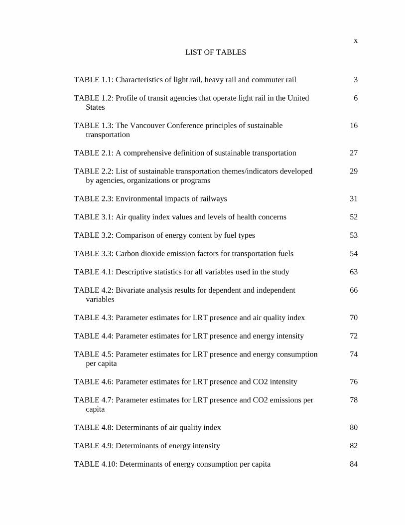
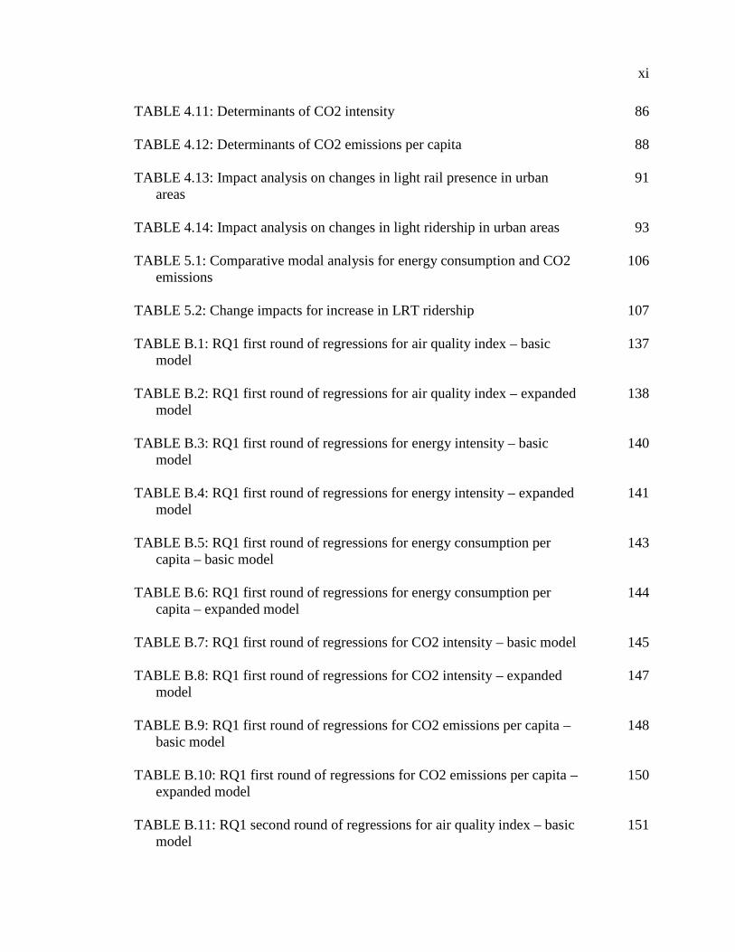
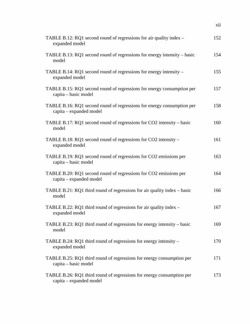
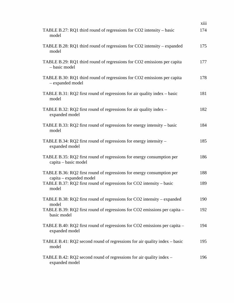
LIST OF TABLES x
LIST OF FIGURES xvi
LIST OF ABBREVIATIONS xviii
CHAPTER 1: INTRODUCTION 1
Background on Sustainability and Sustainable Transportation 5
Perceptions on the Sustainability of Light Rail 8
Statement of the Problem 10
Research Goals and Strategy 11
Theory Base for Research 14
Significance of the Study 19
Overview of the Dissertation Chapters 20
CHAPTER 2: REVIEW OF RELATED LITERATURE 23
Defining Sustainable Transportation 23
Assessment and Measurement of Sustainable Transportation 28
Focus on Environmental Sustainability Assessment 31
Relevant Studies on Light Rail Transit Systems 34
General Findings of the Literature Review 37
CHAPTER 3: METHODOLOGY 40
Research Design 40
Methods of Analysis 42
Model Specifications 46
Variables 48
viii
Data Collection, Preparation and Analysis 51
Chapter Summary 59
CHAPTER 4: PRESENTATION OF THE RESULTS OF ANALYSIS 61
Descriptive Statistics 62
Bivariate Analysis Results 64
Regression Analysis Results 69
Research Question #1: Regression Analysis for All Urban Areaswith LRT
70
Research Question #2: Regression Analysis for Urban Areas 80
Impact Analysis Results 90
Chapter Summary 95
CHAPTER 5: DISCUSSION OF RESULTS 96
Validating the Hypothesis 98
Policy Implications 100
CHAPTER 6: SUMMARY, CONCLUSIONS ANDRECOMMENDATIONS
109
Summary 109
Conclusions 110
Policy Recommendations 111
Limitations of the Study 113
Suggestions for Further Research 116
Final Note 117
REFERENCES 118
APPENDIX A: BIVARIATE FIT ANALYSIS RESULTS 123
ix
APPENDIX B: SUMMARY OF REGRESSION ANALYSIS RESULTS 137
Research Question #1: How does light rail presence affectenvironmental sustainability indicators in urban areas?
137
Research Question #2: For urban areas that have light rail transitsystems, how to light rail, public transit, and urban areacharacteristics affect environmental sustainability indicators?
181
x
LIST OF TABLES
TABLE 1.1: Characteristics of light rail, heavy rail and commuter rail 3
TABLE 1.2: Profile of transit agencies that operate light rail in the UnitedStates
6
TABLE 1.3: The Vancouver Conference principles of sustainabletransportation
16
TABLE 2.1: A comprehensive definition of sustainable transportation 27
TABLE 2.2: List of sustainable transportation themes/indicators developedby agencies, organizations or programs
29
TABLE 2.3: Environmental impacts of railways 31
TABLE 3.1: Air quality index values and levels of health concerns 52
TABLE 3.2: Comparison of energy content by fuel types 53
TABLE 3.3: Carbon dioxide emission factors for transportation fuels 54
TABLE 4.1: Descriptive statistics for all variables used in the study 63
TABLE 4.2: Bivariate analysis results for dependent and independentvariables
66
TABLE 4.3: Parameter estimates for LRT presence and air quality index 70
TABLE 4.4: Parameter estimates for LRT presence and energy intensity 72
TABLE 4.5: Parameter estimates for LRT presence and energy consumptionper capita
74
TABLE 4.6: Parameter estimates for LRT presence and CO2 intensity 76
TABLE 4.7: Parameter estimates for LRT presence and CO2 emissions percapita
78
TABLE 4.8: Determinants of air quality index 80
TABLE 4.9: Determinants of energy intensity 82
TABLE 4.10: Determinants of energy consumption per capita 84
xi
TABLE 4.11: Determinants of CO2 intensity 86
TABLE 4.12: Determinants of CO2 emissions per capita 88
TABLE 4.13: Impact analysis on changes in light rail presence in urbanareas
91
TABLE 4.14: Impact analysis on changes in light ridership in urban areas 93
TABLE 5.1: Comparative modal analysis for energy consumption and CO2emissions
106
TABLE 5.2: Change impacts for increase in LRT ridership 107
TABLE B.1: RQ1 first round of regressions for air quality index – basicmodel
137
TABLE B.2: RQ1 first round of regressions for air quality index – expandedmodel
138
TABLE B.3: RQ1 first round of regressions for energy intensity – basicmodel
140
TABLE B.4: RQ1 first round of regressions for energy intensity – expandedmodel
141
TABLE B.5: RQ1 first round of regressions for energy consumption percapita – basic model
143
TABLE B.6: RQ1 first round of regressions for energy consumption percapita – expanded model
144
TABLE B.7: RQ1 first round of regressions for CO2 intensity – basic model 145
TABLE B.8: RQ1 first round of regressions for CO2 intensity – expandedmodel
147
TABLE B.9: RQ1 first round of regressions for CO2 emissions per capita –basic model
148
TABLE B.10: RQ1 first round of regressions for CO2 emissions per capita –expanded model
150
TABLE B.11: RQ1 second round of regressions for air quality index – basicmodel
151
xii
TABLE B.12: RQ1 second round of regressions for air quality index –expanded model
152
TABLE B.13: RQ1 second round of regressions for energy intensity – basicmodel
154
TABLE B.14: RQ1 second round of regressions for energy intensity –expanded model
155
TABLE B.15: RQ1 second round of regressions for energy consumption percapita – basic model
157
TABLE B.16: RQ1 second round of regressions for energy consumption percapita – expanded model
158
TABLE B.17: RQ1 second round of regressions for CO2 intensity – basicmodel
160
TABLE B.18: RQ1 second round of regressions for CO2 intensity –expanded model
161
TABLE B.19: RQ1 second round of regressions for CO2 emissions percapita – basic model
163
TABLE B.20: RQ1 second round of regressions for CO2 emissions percapita – expanded model
164
TABLE B.21: RQ1 third round of regressions for air quality index – basicmodel
166
TABLE B.22: RQ1 third round of regressions for air quality index –expanded model
167
TABLE B.23: RQ1 third round of regressions for energy intensity – basicmodel
169
TABLE B.24: RQ1 third round of regressions for energy intensity –expanded model
170
TABLE B.25: RQ1 third round of regressions for energy consumption percapita – basic model
171
TABLE B.26: RQ1 third round of regressions for energy consumption percapita – expanded model
173
xiii
TABLE B.27: RQ1 third round of regressions for CO2 intensity – basicmodel
174
TABLE B.28: RQ1 third round of regressions for CO2 intensity – expandedmodel
175
TABLE B.29: RQ1 third round of regressions for CO2 emissions per capita– basic model
177
TABLE B.30: RQ1 third round of regressions for CO2 emissions per capita– expanded model
178
TABLE B.31: RQ2 first round of regressions for air quality index – basicmodel
181
TABLE B.32: RQ2 first round of regressions for air quality index –expanded model
182
TABLE B.33: RQ2 first round of regressions for energy intensity – basicmodel
184
TABLE B.34: RQ2 first round of regressions for energy intensity –expanded model
185
TABLE B.35: RQ2 first round of regressions for energy consumption percapita – basic model
186
TABLE B.36: RQ2 first round of regressions for energy consumption percapita – expanded model
188
TABLE B.37: RQ2 first round of regressions for CO2 intensity – basicmodel
189
TABLE B.38: RQ2 first round of regressions for CO2 intensity – expandedmodel
190
TABLE B.39: RQ2 first round of regressions for CO2 emissions per capita –basic model
192
TABLE B.40: RQ2 first round of regressions for CO2 emissions per capita –expanded model
194
TABLE B.41: RQ2 second round of regressions for air quality index – basicmodel
195
TABLE B.42: RQ2 second round of regressions for air quality index –expanded model
196
xiv
TABLE B.43: RQ2 second round of regressions for energy intensity – basicmodel
198
TABLE B.44: RQ2 second round of regressions for energy intensity –expanded model
199
TABLE B.45: RQ2 second round of regressions for energy consumption percapita – basic model
201
TABLE B.46: RQ2 second round of regressions for energy consumption percapita – expanded model
202
TABLE B.47: RQ2 second round of regressions for CO2 intensity – basicmodel
204
TABLE B.48: RQ2 second round of regressions for CO2 intensity –expanded model
205
TABLE B.49: RQ2 second round of regressions for CO2 emissions percapita – basic model
207
TABLE B.50: RQ2 second round of regressions for CO2 emissions percapita – expanded model
208
TABLE B.51: RQ2 third round of regressions for air quality index – basicmodel
209
TABLE B.52: RQ2 third round of regressions for air quality index –expanded model
211
TABLE B.53: RQ2 third round of regressions for energy intensity – basicmodel
212
TABLE B.54: RQ2 third round of regressions for energy intensity –expanded model
213
TABLE B.55: RQ2 third round of regressions for energy consumption percapita – basic model
215
TABLE B.56: RQ2 third round of regressions for energy consumption percapita – expanded model
216
TABLE B.57: RQ2 third round of regressions for CO2 intensity – basicmodel
218
TABLE B.58: RQ2 third round of regressions for CO2 intensity – expanded 219

xv
model
TABLE B.59: RQ2 third round of regressions for CO2 emissions per capita– basic model
221
TABLE B.60: RQ2 third round of regressions for CO2 emissions per capita– expanded model
222
xvi
LIST OF FIGURES
FIGURE 1.1: Visual representation of the three goals of sustainabletransportation
17
FIGURE 3.1: Analysis map for the assessment of the environmentalsustainability of light rail transit in urban areas
43
FIGURE A.1: Bivariate fit for air quality index and directional route miles 123
FIGURE A.2: Bivariate fit for energy intensity and LRT ridership 124
FIGURE A.3: Bivariate fit for energy intensity and LRT directional routemiles
124
FIGURE A.4: Bivariate fit for energy intensity and LRT operating expenses 125
FIGURE A.5: Bivariate fit for energy intensity and LRT vehicles operatingat maximum service
125
FIGURE A.6: Bivariate fit for energy intensity and LRT passenger milestraveled
126
FIGURE A.7: Bivariate fit for energy intensity and LRT energyconsumption
126
FIGURE A.8: Bivariate fit for energy intensity and LRT CO2 emissions 127
FIGURE A.9: Bivariate fit for energy consumption per capita andemployment density
127
FIGURE A.10: Bivariate fit for energy consumption per capita and ridership 128
FIGURE A.11: Bivariate fit for energy consumption per capita anddirectional route miles
128
FIGURE A.12: Bivariate fit for energy consumption per capita andoperating expenses
129
FIGURE A.13: Bivariate fit for energy consumption per capita and vehiclesoperating at maximum service
129
FIGURE A.14: Bivariate fit for energy consumption per capita and LRTridership
130
xvii
FIGURE A.15: Bivariate fit for energy consumption per capita and LRToperating expenses
130
FIGURE A.16: Bivariate fit for energy consumption per capita and LRTvehicles operating at maximum service
131
FIGURE A.17: Bivariate fit for CO2 intensity and LRT ridership 131
FIGURE A.18: Bivariate fit for CO2 intensity and LRT directional routemiles
132
FIGURE A.19: Bivariate fit for CO2 intensity and LRT operating expenses 132
FIGURE A.20: Bivariate fit for CO2 intensity and LRT vehicles operatingat maximum service
133
FIGURE A.21: Bivariate fit for CO2 intensity and LRT passenger milestraveled
133
FIGURE A.22: Bivariate fit for CO2 intensity and LRT energyconsumption
134
FIGURE A.23: Bivariate fit for CO2 intensity and LRT CO2 emissions 134
FIGURE A.24: Bivariate fit for CO2 emissions per capita and employmentdensity
135
FIGURE A.25: Bivariate fit for CO2 emissions per capita and directionalroute miles
135
FIGURE A.26: Bivariate fit for CO2 emissions per capita and operatingexpenses
136
FIGURE A.27: Bivariate fit for CO2 emissions per capita and employmentdensity 136
xviii
LIST OF ABBREVIATIONS
AQI air quality index
Btu British thermal unit
BCA benefit-cost analysis
CEA cost-effectiveness analysis
CO2 carbon dioxide
CRT commuter rail transit
CST Center for Sustainable Transportation in Canada
DO Direct operations
DOT Department of Transportation
ECMT European Conference of Ministers of Transport
EIA environmental impact assessments
EPA Environmental Protection Agency
ESCOT Economic Assessment of Sustainability Policies of Transport
EST environmentally sustainable transport
FTA Federal Transit Administration
HRT heavy rail transit
IEA International Energy Agency
LCCA life cycle costs analysis
LRT light rail transit
MCA multi-criteria approaches
NAICS North American Industry Classification System
NTD National Transit Database
xix
OECD Organisation for Economic Co-Operation and Development
OLS ordinary least squares
POV privately owned vehicle
PPP policies, plans and programs
PT purchase transportation
ROW right-of-way
RQ1 research question #1
RQ2 research question #2
SEA strategic environmental assessments
SPARTACUS Systems for Planning and Research in Towns and Cities for UrbanSustainability
UNCED United Nations Conference on Environment and Development
UPT unlinked passenger miles
UZA urbanized area
VOMS vehicles operating at maximum service
WCED World Commission on Environment and Development
1
CHAPTER 1: INTRODUCTION
Among all forms of passenger rail, the light rail transit is perceived to be a
sustainable public transit option and an alternative to automobile use, bus systems,
commuter and heavy rail, and other special transportation services. Rail, in general, is a
fuel efficient transport mode especially in comparison to cars and trucks, because of its
capability to transport more passengers or goods (in the case of freight rail systems) to
destinations, which results in less fuel use per miles traveled and less carbon dioxide
emissions (Fietelson, 1994). Passenger rail, in the form of light rail, heavy rail and
commuter rail, is designed to serve local and regional transportation networks in high
frequency and higher ridership levels (Arndt, Morgan, Overman, Clower, Weinstein, &
Seman, 2009). Light rail and heavy rail are both electric rail services and serve local
networks with typical distances of around one mile in between stops. They differ in the
volume of passenger capacities, loading platforms and rights-of-way. However,
compared to commuter rail, light rail and heavy rail services are concentrated on the
central business area. Commuter rail serve local short distance travel between central
city and adjacent suburbs, integrating passengers in various parts of urban areas that use
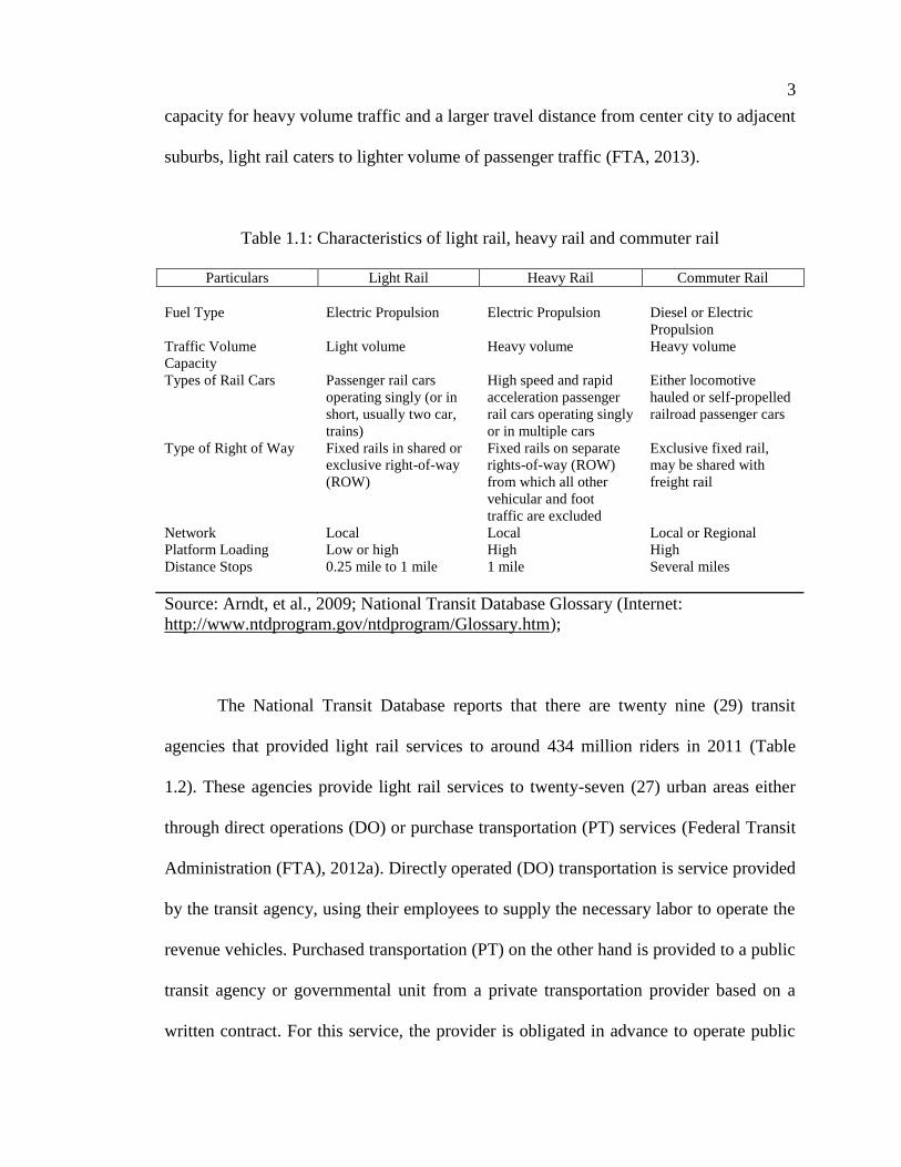
public transit – whether bus, rail or special transportation services. Table 1.1 provides a
comparison of the basic characteristics of light, heavy and commuter rail as defined in
the National Transit Database (Federal Transit Administration (FTA), 2013).
Among all forms of passenger rail, the light rail transit is perceived to be a
sustainable public transit option and an alternative to automobile use, bus systems,
2
commuter and heavy rail, and other special transportation services. This perception is
based on the notion that light rail characteristics adhere to sustainable transportation
principles and that light rail has the ability to address economic, social and
environmental goals that are geared towards ensuring that resources are available for
future generations. Supported by various studies on rail transit benefits (Newman &
Kenworthy, 1999; Schiller, Bruun, & Kenworthy, 2010; Litman, 2012a), light rail has
the potential to solve urban congestion and pollution problems, reduce petroleum
independence, and promote efficient urban development patterns. Light rail
characteristics concur with the sustainable development and sustainable transportation
agenda, which calls for development that is transit-oriented, with transit options that are
competitive with automobiles, with transportation options that reduce energy use,
emissions, noise and other externalities, and with development that encourages efficient
use of urban space (Newman & Kenworthy, 1999). Light rail transit has a positive
influence on increasing transit ridership, reducing traffic congestion, and other
economic, social and environmental benefits, including reducing greenhouse gas
emissions, and less dependence on automobiles especially in urban sprawl areas
(Litman, 2012a).
Light rail, as defined by the Light Rail Transit Subcommittee of the
Transportation Research Board, is “a metropolitan electric railway system characterized
by its ability to operate single cars or short trains along exclusive rights-of-way at
ground level, on aerial structures, in subways, or occasionally, in streets, and to board
and discharge passengers at track or car floor level” (European Conference of Ministers
of Transport (ECMT), 1994). Compared to commuter rail and heavy rail, which has
3
capacity for heavy volume traffic and a larger travel distance from center city to adjacent
suburbs, light rail caters to lighter volume of passenger traffic (FTA, 2013).
Table 1.1: Characteristics of light rail, heavy rail and commuter rail
Particulars Light Rail Heavy Rail Commuter Rail
Fuel Type Electric Propulsion Electric Propulsion Diesel or ElectricPropulsion
Traffic VolumeCapacity
Light volume Heavy volume Heavy volume
Types of Rail Cars Passenger rail carsoperating singly (or inshort, usually two car,trains)
High speed and rapidacceleration passengerrail cars operating singlyor in multiple cars
Either locomotivehauled or self-propelledrailroad passenger cars
Type of Right of Way Fixed rails in shared orexclusive right-of-way(ROW)
Fixed rails on separaterights-of-way (ROW)from which all othervehicular and foottraffic are excluded
Exclusive fixed rail,may be shared withfreight rail
Network Local Local Local or RegionalPlatform Loading Low or high High HighDistance Stops 0.25 mile to 1 mile 1 mile Several miles
Source: Arndt, et al., 2009; National Transit Database Glossary (Internet:http://www.ntdprogram.gov/ntdprogram/Glossary.htm);
The National Transit Database reports that there are twenty nine (29) transit
agencies that provided light rail services to around 434 million riders in 2011 (Table
1.2). These agencies provide light rail services to twenty-seven (27) urban areas either
through direct operations (DO) or purchase transportation (PT) services (Federal Transit
Administration (FTA), 2012a). Directly operated (DO) transportation is service provided
by the transit agency, using their employees to supply the necessary labor to operate the
revenue vehicles. Purchased transportation (PT) on the other hand is provided to a public
transit agency or governmental unit from a private transportation provider based on a
written contract. For this service, the provider is obligated in advance to operate public
4
transportation services for a specific monetary consideration using its own employees to
operate revenue vehicles (FTA, 2013). Total service routes for all urban areas with light
rail cover 807 miles, with light rail from Dallas (Texas), Los Angeles metro area
(California), New York metro area (New York) and San Diego (California) having the
longest routes, and Kenosha (Wisconsin) and Little Rock (Arkansas) with the shortest
routes (Table 1-2). In terms of service area population, the New York-Newark, NY-NJ-
CT urban area has the largest service area population, while Kenosha, WI has the lowest
service area population.
Since the beginning of the light rail movement in North America in the 1960s,
light rail has provided an alternative transport option to bus transit, changed people’s
travel behaviors and improved urban transportation conditions (Thompson, 2003). Urban
development patterns in the 1960s and the 1970s required massive capital improvement
projects for mass transit, like heavy rail, commuter rail and bus systems, to catch up with
urban population growth travel volumes and changing growth patterns in cities. Massive
transportation investments were made, including the construction of the interstate
highway system. In addition, the wave of suburbanization in American cities contributed
to rapid population growth. By the 1980s, the cost of massive capital improvement
projects outpaced available funds for construction of heavy rail and other transportation
projects. Light rail became an adequate and practical alternative to heavy rail. With
funding available through the Federal Transit Administration, and with project
conditions that indicate need, based on urban densities, travel volumes and growth
patterns, light rail construction increased during the period. Light rail, when available in
urban areas, became the most diversified and competitive transportation mode compared

5
to the use of automobile with respect to passenger appeal, speed and positive
environmental impacts (Vuchic, 1999; Greenberg, 2005).
Background on Sustainability and Sustainable Transportation
By the 1990s, the idea of sustainability emerged from discussions organized by
the United Nations World Commission on Environment and Development (WCED) in
1987, the United Nations Conference on Environment and Development (UNCED) in
1992, and in succeeding initiatives by the Organisation for Economic Co-Operation and
Development (OECD) in the late 1990s. The WCED, more popularly known as the
Brundtland Commission, defined sustainable development as “development that meets
the needs of the present without compromising the ability of future generations to meet
their own needs” (WCED, 1987). The concept of sustainability is initially based on
concerns on providing for the needs of future generations and then evolved into a
discussion on developing policy frameworks that address various sectors of society and
covering economic, social and environmental issues. These three issues became the
“triple bottom line” of sustainability – economic, social and environmental
sustainability. This approach made policy discussions and sustainability initiatives more
manageable than the dealing with the overarching intergenerational idea of sustainable
development.
6
Table 1.2: Profile of transit agencies that operate light rail in the United States
Transit Agency Urbanized Area Served
Length ofServiceRoute
(in miles)
Maryland Transit Administration Baltimore, MD 28.8Massachusetts Bay Transportation Authority Boston, MA-NH-RI 25.5Niagara Frontier Transportation Authority Buffalo, NY 6.2Charlotte Area Transit System Charlotte, NC-SC 9.3The Greater Cleveland Regional TransitAuthority
Cleveland, OH 15.2
Dallas Area Rapid Transit Dallas-Fort Worth-Arlington, TX
71.8
Denver Regional Transportation District Denver-Aurora, CO 35.0Metropolitan Transit Authority of HarrisCounty, Texas
Houston, TX 7.4
Kenosha Transit Kenosha, WI-IL 1.0Central Arkansas Transit Authority Little Rock, AR 1.9Los Angeles County MetropolitanTransportation Authority
Los Angeles-LongBeach-Anaheim, CA
60.6
Memphis Area Transit Authority Memphis, TN-MS-AR 5.0Metro Transit Minneapolis-St. Paul,
MN-WI12.4
New Orleans Regional Transit Authority New Orleans, LA 12.7New Jersey Transit Corporation New York-Newark, NY-
NJ-CT58.1
Southeastern Pennsylvania TransportationAuthority
Philadelphia, PA-NJ-DE-MD
41.2
Valley Metro Rail, Inc. Phoenix-Mesa, AZ 19.6Port Authority of Allegheny County Pittsburgh, PA 23.7Tri-County Metropolitan TransportationDistrict of Oregon
Portland, OR-WA 52.2
Sacramento Regional Transit District Sacramento, CA 36.9Utah Transit Authority Salt Lake City-West
Valley City, UT35.4
San Diego Metropolitan Transit System San Diego, CA 54.0North County Transit District San Diego, CA 44.0San Francisco Municipal Railway San Francisco-Oakland,
CA41.6
Santa Clara Valley Transportation Authority San Jose, CA 40.5King County Department of Transportation- Metro Transit Division
Seattle, WA 1.5
Central Puget Sound Regional TransitAuthority
Seattle, WA 17.5
Bi-State Development Agency St. Louis, MO-IL 45.6Hillsborough Area Regional TransitAuthority
Tampa-St. Petersburg, FL 2.4
Source: National Transit Database (Federal Transit Administration, 2010-2011
7
Table 1.2: (continued)Notes:
1. Light rail services are either directly operated (DO) or purchased transportation (PT). DirectlyOperated (DO) Transportation is service provided directly by a transit agency, using theiremployees to supply the necessary labor to operate the revenue vehicles. Purchased transportation(PT) is service provided to a public transit agency or governmental unit from a public or privatetransportation provider based on a written contract. The provider is obligated in advance tooperate public transportation services for a public transit agency or governmental unit for aspecific monetary consideration, using its own employees to operate revenue vehicles. (NationalTransit Database Glossary, FTA, 2012).
2. Ridership data is data from annual unlinked passenger trips from the National Transit Database(FTA, 2012). Ridership for Kenosha, Memphis, New Orleans, and Tampa are based on 2010data. Data for 2011 is not available at the time data is collected.
3. Length of service route is from data from directional route miles from the National TransitDatabase (FTA, 2012). Directional route mile is the mileage in each direction over which publictransportation vehicles travel while in revenue service. One direction of the public transportationvehicles travel while in revenue service. One direction of the directional route miles is the lengthof service route.
In the UNCED conference held in Rio de Janeiro (Brazil) in 1992, national
governments endorsed Agenda 21, which states that “various sectors of human activity
should develop in a sustainable manner”. One of the key sectors that were identified is
transportation. The transportation sector became important because of concerns on how
unsustainable the existing transportation systems are due to growth in transport activity,
use of fossil fuels, air pollution, other environmental issues, and costs of motorized
transport. The growth of transport activity over the years outweighed improvements in
fuel efficiency and the control of emissions (Black W. R., 1996; Organisation for
Economic Co-Operation and Development (OECD), 1997). These concerns became the
driving force for including transportation in the sustainability agenda. Sustainable
transportation, hence, became the expression of sustainable development in the transport
sector. With consideration to the “triple bottom line of sustainability”, transportation
options, such as cars, freight trucks, and public transit options, like bus and passenger
rail, are usually analyzed and assessed based on their respective impacts on society, the
economy and the environment.
8
Perceptions on the sustainability of light rail
Light rail concurs with the broad sustainability agenda for the following reasons
(Newman & Kenworthy, 1999): its competitiveness with the use of automobiles for
private transportation, its compatibility with the use of bicycles as an alternative mode of
transportation, and its attractiveness to pedestrian and transit-oriented development that
promotes appeal and livability in a local area. Because light rail is operated on
electricity, which is a renewable source of energy, light rail is considered a faster and
quieter mode of transport that has less local emissions compared to other forms of
transit. In addition, light rail is flexible, can operate on existing transportation
infrastructure and is adaptable in terms of passenger carrying capacity. Compared to
construction costs and overall transit investment, light rail is a less expensive option than
heavy rail or highway construction (Newman & Kenworthy, 1999). Other positive
attributes of the light rail system also include functionality, quality, safety and reliability
(Cervero, 1984; Newman & Kenworthy, 1999; Vuchic, 1999). Attributes of the light rail
also satisfy criteria for an environmentally conscious public transportation, which
considers transit facilities that are designed to influence sustainable development
patterns, and emphasizes long-term environmental sustainability that reflects
environmentally sound practices (Meyer, 2008). Light rail is considered as sustainable
because of the system’s potential to solve urban congestion and pollution problems,
reduce petroleum independence and promote efficient development patterns. The
permanence of rail transit lines and stations help generate the creation of attractive
human environments, residential developments and business opportunities (Schiller,
Bruun, & Kenworthy, 2010).

9
Despite the adoption, operation and competitiveness of light rail with other forms
of transit, a number of critics have argued that the high initial costs to build the
infrastructure, low ridership, the lack of return on investments and the opportunity cost
for investing in other transportation services (like bus and other special transportation
services, make light rail unsustainable. Case studies on selected operational light rail
systems indicate that light rail may be less efficient, has higher opportunity costs and
lower patronage levels (Gomez-Ibanez, 1985; Fielding, 1995). The opportunity cost for
building other transit options, such as bus services, along with the value for money
service capacity, affordability, flexibility and network coverage of light rail were also
questioned (Semmens, 2006; Hensher, 2007). Critics also argue that light rail, in general,
is outdated, has less ridership, is less cost effective, ineffective in terms of reducing
congestion and emissions, inefficient, more expensive than bus operations, and does not
benefit the poor (as presented in Litman, 2012b). This dissertation hopes to provide
insights on the environmental impacts of light rail and how light rail affects
environmental sustainability.
Rail transit experts, advocates and critics have differing views on the benefits of
light rail as a sustainable transit option for urban areas. These opposing views, however,
indicate room for additional discussions on the advantages and disadvantages of having
a light rail service in the urban area. These discussions from various points of views lead
to understanding and new knowledge on the many aspects of sustainability and
sustainable transportation. Analysis on the different aspects of sustainability enriches the
discussion and improves the literature on assessing sustainable transportation. Since the
sustainable transportation concept emerged from concerns over the environment, a study
10
focusing on light rail, being a sustainable transit option (as described), and how it
specifically affects environmental sustainability can enhance and contribute to existing
comprehensive assessment in the literature of light rail systems as a sustainable transit
option in all sustainability aspects.
Statement of the problem
While there are comprehensive reviews of rail transit benefits in the literature
(Litman, 2012a), empirical studies that have been conducted do not directly addresses
light rail and its environmental sustainability benefits. Granting that sustainability and
sustainable transportation are broad areas for discussion, a targeted and a more specific
approach is needed to address the common perception and arguments for and against the
environmental benefits of light rail in the urban area. Since the concept of sustainable
transportation emerged from environmental concerns brought by transport activities,
focus on the environmental aspect of sustainability is important. Key questions that need
to be answered in addressing common perception on the sustainability of light rail
include the following: Does light rail presence in urban areas contribute to
environmental sustainability? Do other forms of passenger rail contribute to
environmental sustainability? What is environmental sustainability and how is it
measured? Aside from light rail presence, what other factors affect environmental
sustainability indicators? A study on the impact of light rail presence in the urban areas
can address these questions. In addition, identifying factors that affect environmental
sustainability goals and indicators can provide us with additional understanding on the
influence of light rail. Consequently, an empirical analysis can also provide insights on
the plausibility of the differing perceptions on the environmental benefits of light rail.
11
This study hopes to address these issues and provide useful recommendations for
sustainable transportation planning and policy.
Research Goals and Strategy
The primary goal of this research study is to provide an understanding of the
influence of light rail presence on selected environmental sustainability indicators. The
research questions for this study are expressed as follows:
1. How does light rail presence affect environmental sustainability indicators in
urban areas?
2. For urban areas that have light rail systems, how do light rail, public transit,
and urban area characteristics affect environmental sustainability indicators?
To determine how light rail contributes to environmental sustainability,
environmental sustainability goals must be first identified, and matched with many
possible factors that can explain these goals. While the precise definition for
environmental sustainability is evolving with the introduction of many theoretical
frameworks and metrics (Shane & Graedel, 2000; Joumard, 2011; Joumard,
Gudmundsson, & Folkeson, 2011), the goals of environmental sustainability (Hall,
2006) can be summarized as follows:
• minimizing health and environmental damage;
• maintaining high environmental quality and human health standards;
• minimizing the production of noise;
• minimizing the use of land for transportation infrastructure;
• limiting the emissions and waste to levels within the planet’s absorptive
capacity;
12
• ensuring that renewable resources are managed and used in ways that do not
diminish the capacity of ecological systems to continue providing these
resources;
• ensuring that non-renewable resources are used at or below the rate of
development of renewable substitutes;
• ensuring that energy used is powered by renewable energy sources; and
• increasing recycling.
These goals address the negative environmental externalities associated with
transportation: air pollution, consumption of land/urban sprawl, depletion of the ozone
layer, disruption of ecosystems and habitats, climate change, light, noise, vibration, and
water pollution, release of toxic and hazardous substances, solid waste, and depletion of
non-renewable resources and energy supplies (Black W. R., 1996; Black & Sato, 2007;
Hall, 2006; Environmental Protection Agency, 1996; Fietelson, 1994). While the goals
are broad and measurement can be complex with many different variables to represent
environmental issues (Etsy, Levy, Srebotnjak, & De Sherbinin, 2005), the environmental
sustainability goals covered in this study are focused on minimizing pollution,
minimizing energy resource use, and minimizing greenhouse gas emissions. These goals
address the primary concerns that make existing transportation systems unsustainable.
Indicators that represent these goals that are currently available and applicable to urban
areas in the United States include air quality index (for minimizing air pollution), energy
intensity and energy consumption per capita (for minimizing energy consumption), and
carbon dioxide (CO2) emissions intensity and CO2 emissions per capita (for minimizing
greenhouse gas emissions).
13
Possible determinants of environmental sustainability may include light rail,
public transit and urban area characteristics. Urban area characteristics include
metropolitan densities – population density, housing or residential density, and
employment establishment density – which describe urban form. Urban form is the
characterization of the built environment based on its constituent attributes and its
mutual relations (Van Diepen & Voogd, 2001). A measure of mobility of people in the
urban area, such as annual passenger miles traveled, can also affect environmental
sustainability (Van Diepen & Voogd, 2001; Black, Paez, & Suthanaya, 2002). Light rail
characteristics that can also affect environmental sustainability which include ridership
(the number of passengers who board public transportation vehicles), the length of
transit service routes for each direction, transit operating expenses, and the number of
vehicles operated at maximum service (FTA, 2012a). Energy consumed by the light rail
service and the level of carbon dioxide emissions from electricity used for light rail may
also affect environmental sustainability. Aside from the presence of light rail, the
presence of other forms of transit such as commuter rail and heavy rail are also included
as determining factors for comparison.
The impacts of the relationship among these variables, with corresponding
measurement indicators at the urban area level, can be estimated through a series of
regression models, statistical analysis and impact analysis for changes in significant
variables. This research strategy will provide an insight on how light rail presence
contributes to the environmental sustainability in urban areas. The two research
questions articulate the analytical framework for developing a model for assessment of
14
environmental sustainability indicators in urban areas. The results of the analysis are
expected to test and validate the following hypothesis:
1. Light rail presence in urban areas has a significant influence on minimizing
air pollution, energy use and greenhouse gas emissions.
2. Light rail characteristics affect environmental sustainability goals.
3. Public transit characteristics affect environmental sustainability goals.
4. Urban densities affect environmental sustainability goals.
Under the sustainable transportation agenda, the results of this study demonstrate the
relationship between light rail presence and selected environmental sustainability
indicators. The results provide insights on identifying appropriate measures to represent
environmental sustainability goals. While the objective of the analysis does not directly
try to predict selected environmental sustainability indicators based on all the identified
factors, the results of the study may validate this method and approach for sustainability
assessment.
Theory Base for Research
The theoretical basis for this study is rooted on sustainable development and
sustainable transportation. Sustainability has evolved from concerns on the impact of
human activities on the environment to a more focused, issue-based discussion on the
economic, social and environmental dimensions of sustainable development. The
sustainability science covers an interdisciplinary approach to understanding the global,
social and human systems that are crucial to the coexistence of human beings and the
environment (Komiyama & Kazuhiko, 2006). Since the WCED defined sustainable
development as “development that meets the needs of the present without compromising
15
the ability of future generations to meet their own needs” (WCED, 1987), this concept
became a global mission. With the adoption of Agenda 21, sectoral focus is highlighted
in all sustainability initiatives. Sustainable transportation became an expression of
sustainable development in the transportation sector (OECD, 1997).
Sustainable transportation became part of the transportation policy agenda
because of concerns on the unsustainability of existing transportation systems brought by
the growth in transport activity, dependence on finite fossil fuel sources, air pollution
from transport, other environmental issues concerning transportation and costs
associated with motorized transportation (Black, 1996; OECD, 1997), energy resource
consumption and institutional failures (Greene & Wegener, 1997). Intergenerational
equity and the continuance of transportation for future generations also raises an issue
affecting sustainability in transportation (Richardson, Toward a Policy on a
Sustainability Transportation System, 1999). Succeeding studies further expanded the
list of factors that make transportation systems unsustainable: fuel depletion, local
atmospheric effects of motor vehicle emissions, lack of access, congestion,
environmental degradation, vehicle crashes, personal injuries and fatalities (Richardson,
2005; Black & Sato, 2007). Understanding the factors that make transportation systems
unsustainable led to many formulations of the definitions of sustainable transportation. A
set of sustainable transportation principles was presented and endorsed in the Vancouver
Conference organized by the OECD in 1996, which covered principles of access,
decision-making, urban planning, environmental protection, and economic viability.
Table 1-3 presents a summary of these principles (OECD, 1997).
16
Table 1.3: The Vancouver Conference principles of sustainable transportation
Principles Description
Access Improve access to people, goods, and services, but reduce demand for physicalmovement of people and things.
Decision-making Make transportation decisions in an open and inclusive manner that considers allimpacts and reasonable options.
Urban planning Limit sprawl, ensure local mixes of land uses, fortify public transport, facilitatewalking and bicycling, protect ecosystems, heritage, and recreational facilities, andrationalize goods movement.
Environmentalprotection
Minimize emissions and reduce waste from transport activity, reduce noise and useof non-renewable resources, particularly fossil fuels, and ensure adequate capacityto respond to spills and other accidents.
Economic viability Internalize all external costs of transport including subsidies but respect equityconcerns, promote appropriate research and development, consider the economicbenefits including increased employment that might result from restructuringtransportation, and form partnerships involving developed and developingcountries for the purpose of creating and implementing new approaches tosustainable transportation.
Source: Organisation for Economic Co-Operation and Development (OECD), 1997.
As a response to the challenge of developing the concept of sustainable
transportation, definitions based on the principles agreed at the Vancouver Conference in
1996 were developed by the Center for Sustainable Transportation in Canada (CST) in
1997, which was also later adapted by the Council of the European Union in 2001. A
sustainable transportation system has the following characteristics:
• “Allows the basic access and development needs of individuals, companies and
society to be met safely and in a manner consistent with human and ecosystem and
health, and promotes equity within and between successive generations;
• Is affordable, operates fairly and efficiently, offers a choice of transport mode and
supports a competitive economy, as well as balanced regional development; and
• Limits emissions and waste within the planet’s ability to absorb them, uses
renewable resourced at or below their rates of generation, and uses non-renewable
resources at or below rates of development of renewable substitutes, while
17
minimizing the impact on the use of land and the generation of noise” (CST, 2002;
CST, 2005; Litman, 2007; Greg, Kimble, Nellthorp, & Kelly, 2010).
Furthermore, CST also developed a visual representation of the linkages between
economy, society and the environment depicting the relationships between the
sustainability goals of economic development and vitality, social equality and well-
being, and environmental preservation and regeneration. Figure 1.1 presents the
convergence of these over-arching goals.
The economy describes the available resources and how resources are organized
to meet human needs and goals. Society, on the one hand, is the composite of human
interactions and how they are organized. The sustainability of societies is a necessary
condition for meeting human needs. Finally, the environment refers to the surroundings
of humans and other life forms that support them and limits their activity according to
Source: The Centre for Sustainable Transportation (CST), 2002
Figure 1.1: Visual representation of the three goals of sustainable transportation
18
basic physical laws (CST, 2002). The goal of sustainable transportation is to address
transport needs by providing access to affordable and efficient transport mode choices
that supports economic development and vitality, environmental preservation and
regeneration, and social equality and well-being (CST, 2002; CST, 2005). While many
definitions, indicators and metrics of sustainable transportation have emerged (Jeon &
Amekudzi, 2005; Hall, 2006), there is a general consensus that a sustainable
transportation system should address all environmental, social and economic
externalities associated with transportation.
Metropolitan growth theories also support the notion of sustainability and
sustainable transportation. Urban planners and local officials are vested in the
preservation and revitalization of central cities that have been affected by
suburbanization and rail transit is one of the transport mechanisms used to facilitate the
mobility of the middle working class from their home to their workplace in center cities.
Rail transit is also promoted for its economic development potential and its potential to
decrease congestion, as well as pollution. Also, rail transit is politically acceptable
compared to highway construction in some cases because of its smaller
environmental/ecological footprint on urban areas. Finally, rail transit supports smart
growth, which regards transit-based accessibility as a key element in fostering high
density development patterns that define modern cities today (Giuliano, 2004).
Environmentally conscious transportation (Meyer, 2008) affects the
intergenerational aspect of sustainable development by making resources available for
use by future generations. In this study, estimating the impact of light rail presence on
the environmental sustainability of urban areas addresses the perception of whether light
19
rail helps lower air pollution, energy use and greenhouse gas emissions in the area.
Understanding these environmental sustainability goals feeds into the comprehensive
understanding of sustainable transportation that is used as a policy framework in transit
planning.
Significance of the Study
The assessment of light rail transit (LRT) systems in the literature has been
focused on the analyses of the attributes of light rail operations, feasibility studies,
capacity studies, efficiency and effectiveness. The approach used by these studies mostly
focuses on case studies or comparative analyses of different light rail systems in the US
using sets of criteria or goals. Conclusions from these studies mostly yield case-specific
results and are dependent on the variability of the conditions and operations associated
with existing operational LRT systems (Greenberg, 2005). An analysis of the viability of
light rail systems under the sustainability framework leads to a better understanding of
how light rail influences environmental sustainability in urban areas.
The primary contribution of this study will be an empirical assessment of the
impact of light rail presence on environmental sustainability indicators. Because
sustainable development is grounded on concerns on the impact of human activities –
including transportation – on the environment, this study focuses on the environmental
aspect of sustainability. While studies on the social and economic aspects of sustainable
transportation are equally important, there is a research gap in analyzing the impact of
passenger rail transit modes to the environmental sustainability in the urbanized area.
Focusing on environmental sustainability, a more specific explanation will be provided
on whether or not the perception for the benefits provided by light rail is valid.
20
Aside from enhancing the current literature on the environmental sustainability
of light rail systems, the results of the analysis assess the viability of the selected
indicators for environmental sustainability goals and identify factors that influence
environmental sustainability. By identifying influential factors, policy can be directed
towards improving these factors so that the benefit of environmental sustainability is
achieved. The results of analysis can be used to aid policy formulation and analysis
through more study of the significant factors that influence environmental sustainability.
The assessment of the impact of light rail presence on environmental
sustainability can also be a starting point to develop an appropriate policy instrument for
evaluating the light rail as a viable and sustainable transit option. Although this study
only focuses primarily on the environmental aspect, the results of the study can also
enrich the existing literature on sustainable transportation and how light rail systems are
evaluated. The methodology used for analyzing the impact of light rail on environmental
sustainability can also be applied to economic and social sustainability outcomes in
future research endeavors. This study can also help strengthen policy discussions that
relate to the principles of sustainable transportation.
Overview of the Dissertation Chapters
The objective of this dissertation is to understand how light rail presence affects
environmental sustainability in urban areas. Environmental sustainability indicators
include measurements for minimizing air pollution, energy resource use and greenhouse
gas emissions. The study is focused on the environmental aspect of sustainable
transportation and will also include the identification of indicators that will best describe
environmental sustainability.
21
To undertake this study on determining the influence of light rail on
environmental sustainability, this dissertation is organized into six chapters that cover
the background of the study, the literature review, the methodology, and the presentation
of the results of the analysis. A discussion of the results and policy implications will also
be included. The concluding chapter will provide the major conclusions of the study and
recommendations for future directions for research on the assessment of the impact of
light rail on environmental sustainability.
Chapter 1 serves as the introductory chapter, which provides the rationale for the
study, the statement of the problem and a brief discussion on sustainability and
sustainable transportation as the theoretical basis for this study. Chapter 1 also states the
research goals, the research questions and the research strategy for this study, the
significance of the study, and the scope and limitations of entire research study. Chapter
2 provides the review of related literature on sustainability, sustainable development and
sustainable transportation. The literature review also includes a review of previous
studies on light rail transit systems and the issue of environmental sustainability
assessment. Chapter 3 focuses on the methodology used in the study, including a
discussion on the research design, the population and sample, variables to be used, data
collection and preparation, as well as the methods used for analysis. Chapter 4 presents
the analysis and the results while Chapter 5 provides a discussion of the results and the
policy implications of the results of the study. Chapter 6 concludes the study and
provides policy recommendations and suggestions for the future direction for research
on environmental sustainability. This study is expected to provide insights on how light
rail presence affects air quality, energy consumption and carbon dioxide emissions.
22
Determinants of these selected environmental sustainability indicators will also be
identified in the study. The conclusions from this study are expected to aid policy
formulation and analysis related to light rail, and also strengthen the discussions on the
issues related to sustainable transportation.
23
CHAPTER 2: REVIEW OF RELATED LITERATURE
This chapter provides an expanded review of the concept of sustainable
development from the definition provided by the Brundtland Commission (WCED,
1987) to a more comprehensive definition of sustainable transportation that covers
economic, social and environmental goals. A discussion of the assessment of sustainable
transportation and the development of selected indicator frameworks is included in this
section followed by a more focused narrative on environmental sustainability. Finally, a
discussion on studies pertaining to light rail transit systems will also be included in this
chapter. Based on these discussions on pertinent literature on environmental
sustainability and light rail systems, the rationale for the formulation of the research
question concludes this chapter.
Defining Sustainable Transportation
Sustainability emerged from discussions organized by the United Nations World
Commission on Environment and Development (WCED) in 1987, the United Nations
Conference on Environment and Development (UNCED) in 1992, and in succeeding
initiatives by the Organisation for Economic Co-Operation and Development (OECD) in
the late 1990s. The WCED, more popularly known as the Brundtland Commission,
defined sustainable development as “development that meets the needs of the present
without compromising the ability of future generations to meet their own needs”
(WCED, 1987). This definition assumed that the existing natural environments can
24
support the increasing human population needs of the present and future generations. In
addition, sustainability in this sense addresses the issue of equity and equity among
populations in present and future generations, and encompasses the general
understanding of economic, environmental and social aspects. However, criticism for
this definition indicates that sustainability in this sense failed to consider the earth’s
carrying capacity, ecological stability and geographical security (Daly, 1990; Rees,
1995). By the 1990s, following the United Nations Conference on Environment and
Development (UNCED) held in Rio de Janeiro, Brazil in 1992, the attending national
governments endorsed Agenda 21, which states that “various sectors of human activity
should develop in a sustainable manner”. Sustainable transportation, hence, became the
expression of sustainable development in the transport sector, which became the focus of
various international efforts for developing the concept’s definition (OECD, 1997).
To respond to concerns that transportation provides challenges to the sustainable
development agenda, OECD, together with the Government of Canada, organized a
conference on sustainable transportation on March 24 to 27, 1996 in Vancouver, British
Columbia. Key transportation stakeholders from 25 nations developed a vision for
sustainable transportation, bringing to the discussion findings from a series of meetings
between 1990 and 1994 that were organized by the OECD, the International Energy
Agency (IEA), the European Conference of Ministers of Transport (ECMT) and others
agencies and governments. These meetings underlined technical solutions, such as the
development of low consumption and low emission automobiles, promotion of clean
fuel for cars, use of alternative fuel vehicles and provision for public transit as
alternative transportation options. With growing consensus to bring sustainable
25
transportation on the policy agenda, the Vancouver Conference brought together around
400 automobile and alternative vehicle manufacturers, fuel producers, regional and local
planners, and government officials to develop a vision for sustainable transport.
Participants in the conference acknowledged that the challenge is to find ways of
meeting transportation needs that are environmentally sound, socially equitable and
economically viable. A set of sustainable transportation principles (Table 1-3) was
presented and endorsed, which covered principles of access, decision-making, urban
planning, environmental protection, and economic viability.
In the Vancouver Conference, a review of the conditions for sustainable
transportation under the OECD’s Environmentally Sustainable Transport (EST) project
in 1996 also yielded a preliminary qualitative definition of an environmentally
sustainable transport (EST). An environmentally sustainable transportation system is
“transportation that does not endanger public health or ecosystems and meets mobility
needs consistent with (a) use of renewable resources at below their rates of regeneration
and (b) use of non-renewable resources at below the rates of development of renewable
substitutes” (OECD, 1997). This definition, however, focused only on addressing the
environmental goal of sustainable development. The economic and social goals were not
been considered at this 1997 conference.
Sustainable transportation has also been defined as “satisfying current transport
and mobility needs without compromising the ability of future generations to meet their
needs” (Black W. R., 1996). This definition is a broad representation of the transport
sector based on the definition of sustainability from the Brundtland Commission report.
Another definition specifies more details but this is also broadly based on the Brundtland
26
Commission: “a sustainable transportation system is one in which fuel consumption,
vehicle emissions, safety, congestion and social and economic access are at such levels
that they can be sustained into the indefinite future without compromising the ability of
future generations of people throughout the world to meet their transportation needs
(Richardson, 1999).
Finally, the United Nations also proposed that sustainable development when
applied to the transportation sector has to secure a balance between equity, efficiency
and the capacity to answer the needs of future generations. This role implies securing the
energy supply, reflecting the costs of non-renewable resources in transport vehicle
operations, creating responsive and effective markets, and adopting production processes
respective of the environment by eliminating externalities that are detrimental to future
generations (Rodrigue, Comtois, & Slack, 2006).
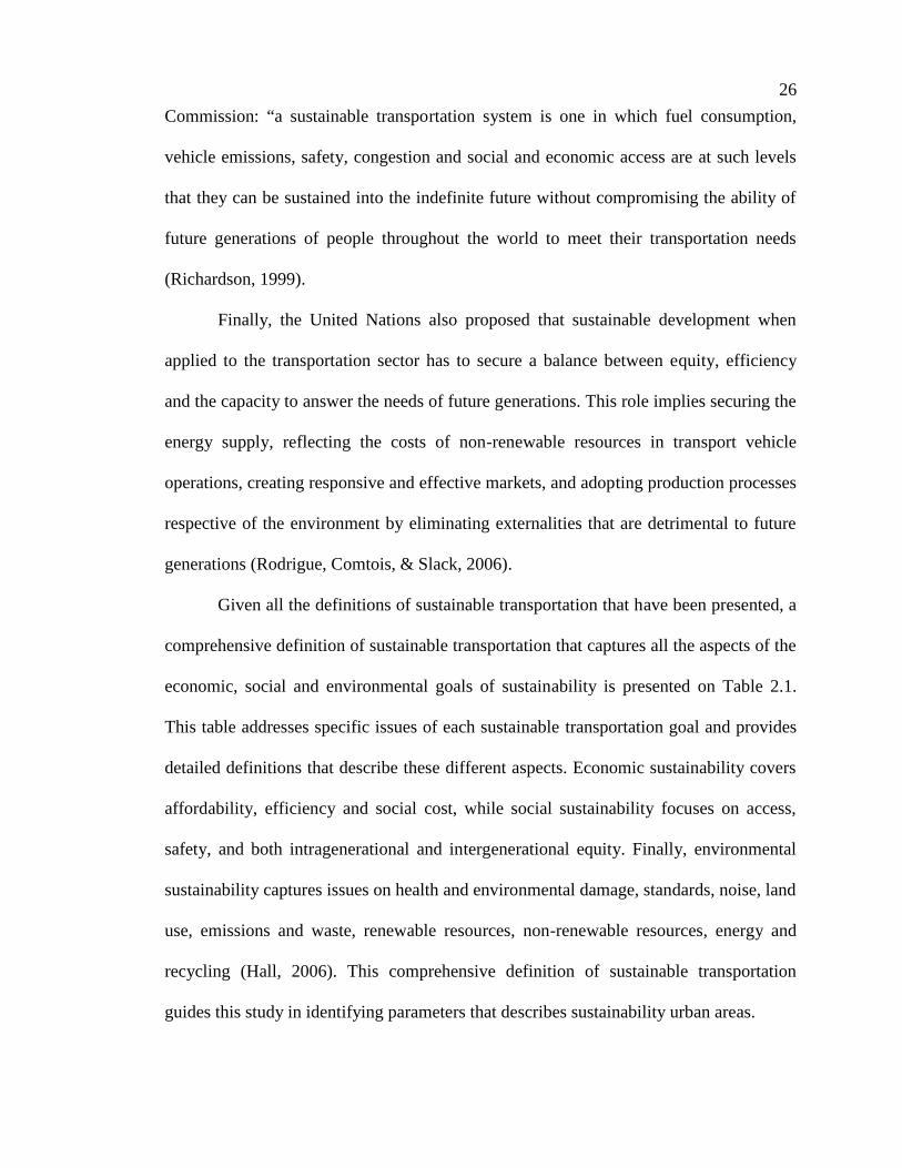
Given all the definitions of sustainable transportation that have been presented, a
comprehensive definition of sustainable transportation that captures all the aspects of the
economic, social and environmental goals of sustainability is presented on Table 2.1.
This table addresses specific issues of each sustainable transportation goal and provides
detailed definitions that describe these different aspects. Economic sustainability covers
affordability, efficiency and social cost, while social sustainability focuses on access,
safety, and both intragenerational and intergenerational equity. Finally, environmental
sustainability captures issues on health and environmental damage, standards, noise, land
use, emissions and waste, renewable resources, non-renewable resources, energy and
recycling (Hall, 2006). This comprehensive definition of sustainable transportation
guides this study in identifying parameters that describes sustainability urban areas.
27
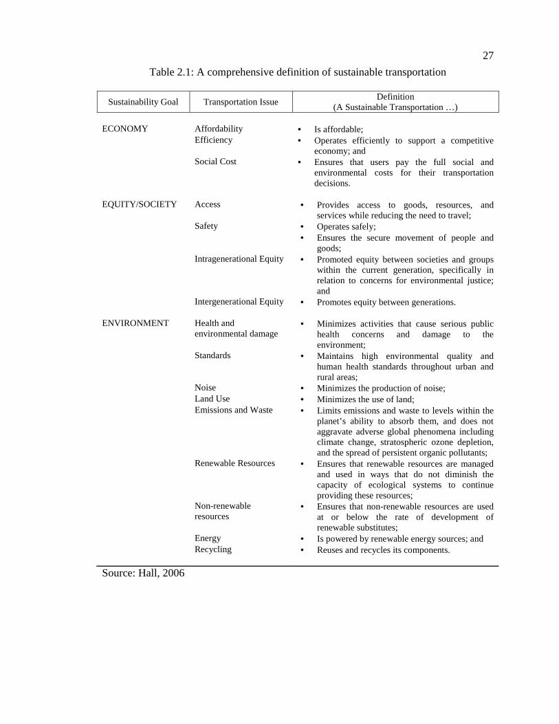
Table 2.1: A comprehensive definition of sustainable transportation
Sustainability Goal Transportation IssueDefinition
(A Sustainable Transportation …)
ECONOMY Affordability • Is affordable;Efficiency • Operates efficiently to support a competitive
economy; andSocial Cost • Ensures that users pay the full social and
environmental costs for their transportationdecisions.
EQUITY/SOCIETY Access • Provides access to goods, resources, andservices while reducing the need to travel;
Safety • Operates safely;• Ensures the secure movement of people and
goods;Intragenerational Equity • Promoted equity between societies and groups
within the current generation, specifically inrelation to concerns for environmental justice;and
Intergenerational Equity • Promotes equity between generations.
ENVIRONMENT Health andenvironmental damage
• Minimizes activities that cause serious publichealth concerns and damage to theenvironment;
Standards • Maintains high environmental quality andhuman health standards throughout urban andrural areas;
Noise • Minimizes the production of noise;Land Use • Minimizes the use of land;Emissions and Waste • Limits emissions and waste to levels within the
planet’s ability to absorb them, and does notaggravate adverse global phenomena includingclimate change, stratospheric ozone depletion,and the spread of persistent organic pollutants;
Renewable Resources • Ensures that renewable resources are managedand used in ways that do not diminish thecapacity of ecological systems to continueproviding these resources;
Non-renewableresources
• Ensures that non-renewable resources are usedat or below the rate of development ofrenewable substitutes;
Energy • Is powered by renewable energy sources; andRecycling • Reuses and recycles its components.
Source: Hall, 2006
28
Assessment and Measurement of Sustainable Transportation
The assessment and measurement of sustainable transportation is as elusive as
finding a standard definition for the concepts of sustainability and sustainable
development. These definitions also evolved from attempts to quantify general
definitions and assign various measurable indicators. This section provides a discussion
on selected tools and approaches for sustainability assessment. These tools and
approaches were designed to aid policy decision-making and to promote sustainable
transportation.
Sustainability assessment is initially driven by environmental impact assessments
(EIAs) and strategic environmental assessments (SEAs). EIAs are typically applied to
project proposals and SEAs are applied to policies, plans and programs (PPPs). EIA-
driven integrated assessments aim to identify the environment, social and economic
impacts of a proposal after a proposal has been designed. Resulting impacts are then
compared with baseline conditions to determine whether or not they are acceptable.
SEA-driven assessments (also referred to as objectives-led integrated assessments) help
determine the extent to which a proposal contributes to defined environmental, social
and economic goals before a proposal has been designed and to determine the “best”
available option in terms of meeting these goals. Both types of assessments reflect the
vision of sustainability but do not determine whether or not an initiative is actually
sustainable. An “assessment for sustainability” approach is proposed that requires a clear
concept of sustainability as a societal goal is defined by criteria against which the
assessment is conducted, and which separates sustainable outcomes from unsustainable
ones. Although this concept has been defined in theory, this concept is not always
29
evident, nor is it applied empirically in practice (Pope, Annandale, & Morrison-
Saunders, 2004).
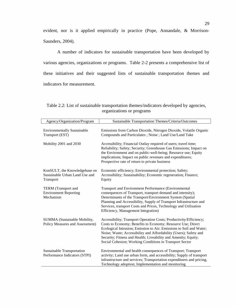
A number of indicators for sustainable transportation have been developed by
various agencies, organizations or programs. Table 2-2 presents a comprehensive list of
these initiatives and their suggested lists of sustainable transportation themes and
indicators for measurement.
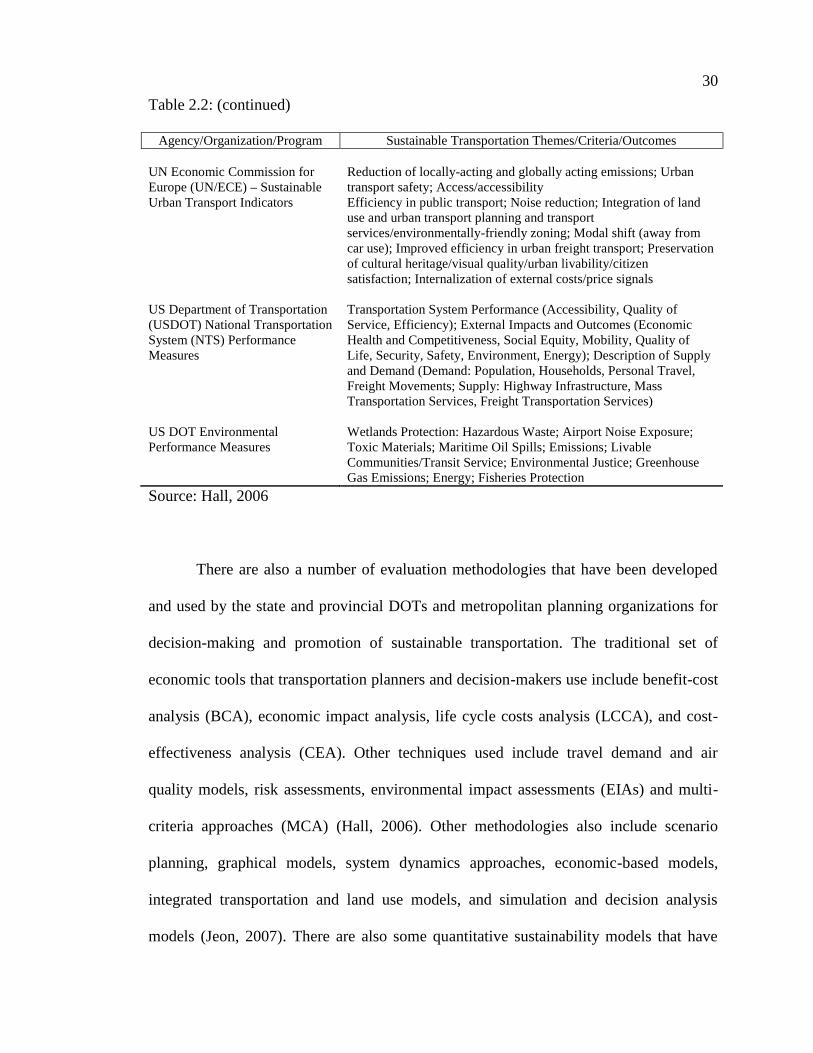
Table 2.2: List of sustainable transportation themes/indicators developed by agencies,organizations or programs
Agency/Organization/Program Sustainable Transportation Themes/Criteria/Outcomes
Environmentally SustainableTransport (EST)
Emissions from Carbon Dioxide, Nitrogen Dioxide, Volatile OrganicCompounds and Particulates ; Noise ; Land Use/Land Take
Mobility 2001 and 2030 Accessibility; Financial Outlay required of users; travel time;Reliability; Safety; Security; Greenhouse Gas Emissions; Impact onthe Environment and on public-well-being; Resource use; Equityimplications; Impact on public revenues and expenditures;Prospective rate of return to private business
KonSULT, the Knowledgebase onSustainable Urban Land Use andTransport
Economic efficiency; Environmental protection; Safety;Accessibility; Sustainability; Economic regeneration; Finance;Equity
TERM (Transport andEnvironment ReportingMechanism
Transport and Environment Performance (Environmentalconsequences of Transport, transport demand and intensity);Determinants of the Transport/Environment System (SpatialPlanning and Accessibility, Supply of Transport Infrastructure andServices, transport Costs and Prices, Technology and UtilisationEfficiency, Management Integration)
SUMMA (Sustainable Mobility,Policy Measures and Assessment)
Accessibility; Transport Operation Costs; Productivity/Efficiency;Costs to Economy; Benefits to Economy; Resource Use; DirectEcological Intrusion; Emission to Air; Emissions to Soil and Water;Noise; Waste; Accessibility and Affordability (Users); Safety andSecurity; Fitness and Health; Liveability and Amenity; Equity;Social Cohesion; Working Conditions in Transport Sector
Sustainable TransportationPerformance Indicators (STPI)
Environmental and health consequences of Transport; Transportactivity; Land use urban form, and accessibility; Supply of transportinfrastructure and services; Transportation expenditures and pricing,Technology adoption; Implementation and monitoring
30
Table 2.2: (continued)
Agency/Organization/Program Sustainable Transportation Themes/Criteria/Outcomes
UN Economic Commission forEurope (UN/ECE) – SustainableUrban Transport Indicators
Reduction of locally-acting and globally acting emissions; Urbantransport safety; Access/accessibilityEfficiency in public transport; Noise reduction; Integration of landuse and urban transport planning and transportservices/environmentally-friendly zoning; Modal shift (away fromcar use); Improved efficiency in urban freight transport; Preservationof cultural heritage/visual quality/urban livability/citizensatisfaction; Internalization of external costs/price signals
US Department of Transportation(USDOT) National TransportationSystem (NTS) PerformanceMeasures
Transportation System Performance (Accessibility, Quality ofService, Efficiency); External Impacts and Outcomes (EconomicHealth and Competitiveness, Social Equity, Mobility, Quality ofLife, Security, Safety, Environment, Energy); Description of Supplyand Demand (Demand: Population, Households, Personal Travel,Freight Movements; Supply: Highway Infrastructure, MassTransportation Services, Freight Transportation Services)
US DOT EnvironmentalPerformance Measures
Wetlands Protection: Hazardous Waste; Airport Noise Exposure;Toxic Materials; Maritime Oil Spills; Emissions; LivableCommunities/Transit Service; Environmental Justice; GreenhouseGas Emissions; Energy; Fisheries Protection
Source: Hall, 2006
There are also a number of evaluation methodologies that have been developed
and used by the state and provincial DOTs and metropolitan planning organizations for
decision-making and promotion of sustainable transportation. The traditional set of
economic tools that transportation planners and decision-makers use include benefit-cost
analysis (BCA), economic impact analysis, life cycle costs analysis (LCCA), and cost-
effectiveness analysis (CEA). Other techniques used include travel demand and air
quality models, risk assessments, environmental impact assessments (EIAs) and multi-
criteria approaches (MCA) (Hall, 2006). Other methodologies also include scenario
planning, graphical models, system dynamics approaches, economic-based models,
integrated transportation and land use models, and simulation and decision analysis
models (Jeon, 2007). There are also some quantitative sustainability models that have
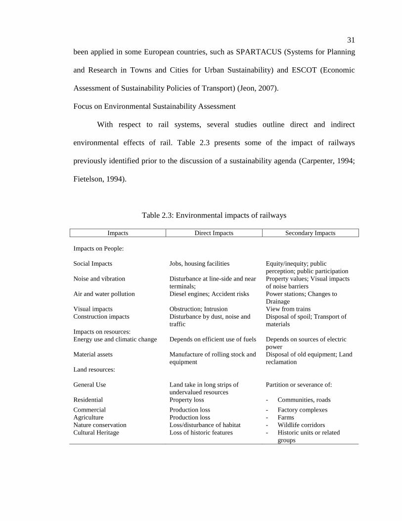
31
been applied in some European countries, such as SPARTACUS (Systems for Planning
and Research in Towns and Cities for Urban Sustainability) and ESCOT (Economic
Assessment of Sustainability Policies of Transport) (Jeon, 2007).
Focus on Environmental Sustainability Assessment
With respect to rail systems, several studies outline direct and indirect
environmental effects of rail. Table 2.3 presents some of the impact of railways
previously identified prior to the discussion of a sustainability agenda (Carpenter, 1994;
Fietelson, 1994).
Table 2.3: Environmental impacts of railways
Impacts Direct Impacts Secondary Impacts
Impacts on People:
Social Impacts Jobs, housing facilities Equity/inequity; publicperception; public participation
Noise and vibration Disturbance at line-side and nearterminals;
Property values; Visual impactsof noise barriers
Air and water pollution Diesel engines; Accident risks Power stations; Changes toDrainage
Visual impacts Obstruction; Intrusion View from trainsConstruction impacts Disturbance by dust, noise and
trafficDisposal of spoil; Transport ofmaterials
Impacts on resources:Energy use and climatic change Depends on efficient use of fuels Depends on sources of electric
powerMaterial assets Manufacture of rolling stock and
equipmentDisposal of old equipment; Landreclamation
Land resources:
General Use Land take in long strips ofundervalued resources
Partition or severance of:
Residential Property loss - Communities, roads
Commercial Production loss - Factory complexesAgriculture Production loss - FarmsNature conservation Loss/disturbance of habitat - Wildlife corridorsCultural Heritage Loss of historic features - Historic units or related
groups
32
Table 2.3: (continued)
Impacts Direct Impacts Secondary Impacts
Amenity Land take - Paths, golf links, playingfields
Scenic Landscape Intrusion; modifications tofeatures
Effects on distant active landforms
Sources: Carpenter, 1994; Fietelson, 1994.
In 1996, the U.S. Environmental Protection Agency (EPA) developed
quantitative national estimates of the impacts of highway, rail, aviation and maritime
transport on the environment. This assessment addressed the full life cycle cost of
transportation, from construction of infrastructure to the manufacture of vehicles and
parts. The study utilized a categorization scheme that focuses on the grouping of the
impacts of basic transportation activities affecting the environment. The basic
transportation activities include the following: a) infrastructure construction,
maintenance, and abandonment; b) vehicle and parts manufacture; c) vehicle travel; d)
vehicle maintenance and support; and e) disposal of used vehicles and parts. This
categorization shifts the focus on transportation activities, rather than on impacts on the
forms of environment such as air, water and land resources (Environmental Protection
Agency, 1996). However, while this study succeeded in identifying environmental
impact indicators, most of the indicators that were identified have limitations on the
availability of data in the transportation statistics that are currently being collected by
government and other statistical agencies. In summary, the EPA’s assessment was
initiated on a completely different empirical basis that may not be easily replicated and a
completely different analytical approach. There has been no other subsequent EPA
study on this topic that can be found in the literature.
33
At the national level, however, an environmental sustainability index developed
by the Yale Center for Environmental Law and Policy was formulated based on five
fundamental components of sustainability: environmental systems, environmental
stresses, human vulnerability to environmental stresses, societal capacity to respond to
environmental challenges, and global stewardship (Etsy, Levy, Srebotnjak, & De
Sherbinin, 2005). By integrating datasets that consider natural resource endowments,
historical pollution levels, environmental management efforts and capacity of the society
to improve environmental performance, 21 indicators that describe environmental
sustainability were identified. These indicators are: air quality, biodiversity, land, water
quality, water quantity, reducing air pollution, reducing ecosystem stresses, reducing
population growth, reducing waste and consumption pressures, reducing water stress,
natural resource management, environmental health, basic human sustenance, reducing
environment-related natural disaster vulnerability, environmental governance, eco-
efficiency, private sector responsiveness, science and technology, participation in
international collaborative efforts, greenhouse gas emissions, and reducing trans-
boundary environmental pressures (Etsy, Levy, Srebotnjak, & De Sherbinin, 2005).
While the study boasts of the richness of specific environmental impact indicators, the
study only focuses on one year, based on national data collected from different countries.
Factors that explained environmental sustainability using this approach are too broad,
and may only be used to explain environmental sustainability in general terms.
Urban environmental sustainability metrics were also defined covering issues
that affect urban areas such as air, water solids, transportation, energy, resource use,
population, urban ecology, livability and general environmental management (Shane &
34
Graedel, 2000). This study identified metrics that were used on a study of Vancouver,
Canada, whose government has embraced sustainability in their urban planning and
policy development. The study provided a good starting point for exploring other metrics
that are issue-based and applicable to urban areas.
Finally, recognizing different ways and approaches in analyzing environmental
sustainability, a new framework is being proposed that takes into account causal chains
on environmental issues in the transport sector (Joumard, 2011; Joumard, Gudmundsson,
& Folkeson, 2011). There are forty nine (49) identified causal chains in the study that
covers the following environmental issues: noise and vibrations, accidents, air pollution,
soil and water pollution, impacts on land, non-renewable resource use and waste
handling, greenhouse effects, and other impacts. While this approach captures several
environmental aspects, an empirical study needs to be done to demonstrate the
assessment of environmental sustainability. The study is still conceptual but it provides
ideas for future research on environmental sustainability, whether applied to public
transit options or as applied to urban areas that currently provide public transit services.
Relevant Studies on Light Rail Transit Systems
Existing relevant light rail studies in the literature focus on the attributes of LRT
operations, capacity studies, efficiency and effectiveness. In terms of its desirable
characteristics, LRT systems are quiet, and environmentally unobtrusive. LRT is
electrically propelled, so the “carbon footprint” of petrochemical fuels is shifted from the
private owned vehicles (POVs), freight and commercial carriers to the electrical power
grid, which is usually in areas some distance from urban centers. They operate
effectively along available railroad tracks and sometimes on street medians. LRT is also
35
cheaper and less disruptive, easier to build than heavy rail, and also lacks exhaust fumes.
LRT runs on slower speeds than heavy rail and is designed for pedestrian settings
(Cervero, 1984). Aside from these characteristics, LRT is also competitively compared
with automobiles in terms of image and functionality. It is also cheaper to build than
new highways. It is attractive to both residential and commercial development, and is
able to “green the city” (Newman & Kenworthy, 1999). LRT is also superior to buses in
terms of riding comfort, vehicle performance and system image (Vuchic, 1999).
There are many studies that have been conducted to assess the performance of
light rail systems. In addition to the pros and cons of investing in light rail systems,
analysis of impacts on land use, residential location and employment location have also
been conducted (Bhatta & Drennan, 2003; Giuliano, 2004). Light rail systems have also
been compared to bus rapid transit systems in terms of operating costs, impacts on
travel, capital costs, and speed (Semmens, 2006), value for money, service capacity,
affordability, relative flexibility and network coverage (Hensher, 2007). A few other
studies were also conducted focusing on planning for the operation of LRT systems,
including urban rail terminal location (Horner & Grubesic, 2001) as well as decision
making processes involving local governments (De Bruijn & Veeneman, 2009).
A study on light rail systems in Europe in comparison with bus systems
demonstrate that there are many system-wide benefits of having LRT systems compared
to only having bus systems (Hass-Klau, Crampton, & Benjari, 2004). Benefits that were
identified in the study were higher public transport patronage, more passengers
transported per hour compared to standard buses, low noise and pollution, running
comfort, better urban design and slightly cheaper cost than buses. In another study that
36
compared 130 US cities with and without rail, those with rail systems have lower traffic
congestion costs, lower traffic fatalities, lower consumer transport expenditures, higher
public transport ridership, higher operating costs per passenger mile and higher public
transport service cost recovery (Litman, 2004). The findings from these studies support
the findings from an international study on the significance of rail in higher income
cities, where cities with strong rail features have greater wealth and more cost-effective
urban transport systems. In relation to environmental factors, the findings of this
international study also yield these conclusions: a) per capita use of energy increases in
private passenger transport as cities are less rail-oriented, and b) per capita generation of
local smog producing emissions from transport are higher in cities with no rail than in
cities with strong rail presence (Kenworthy, 2008).
A more recent study on light rail transit was conducted in Hamilton, Canada,
where health, environmental and economic impacts were reviewed (Topalovic, Carter,
Topalovic, & Krantzberg, 2012).Findings indicate that LRT in medium sized growing
cities like Hamilton are considered as a catalyst for transit-oriented, high density and
mixed use development. In addition, their findings conclude that LRT is an
economically sound investment opportunity, and a catalyst for social change that helps
improve health, environment and connectivity in the community. From this study alone,
it appears that LRT concurs with the sustainable transportation agenda, although its
findings are concentrated on the economic benefits of light rail rather than on
environmental aspects. A related study on Hamilton’s light rail modeled the relationship
between the construction of an LRT network and land use, transportation and other
37
activities (Lavery & Kanaroglou, 2012). They find that construction of an LRT network
alone is not sufficient causation for economic development and transit modal shares.
General Findings of the Literature Review
The literature review tells us that most of the studies cover concepts, definitions
and themes that relate to sustainable transportation. There are studies that pertain to the
measurement of sustainable transportation and environmental sustainability. While there
are relevant studies pertaining to light rail, most of these studies are case studies and
have specific application for selected urban areas. Some literature on rail and light rail
focus on advantages and disadvantages of light rail but findings are biased towards other
public transit modes like buses, and still with automobile use. Studies on the factors that
contribute to environmental sustainability at the urban level are limited, and not entirely
focused on light rail.
Based on the foregoing discussion of the related literature on environmental
sustainability and light rail systems, there are limited empirical studies that directly
focuses on the impact of the implementation of light rail transit systems on
environmental sustainability, and even with comprehensive sustainability. A number of
studies have been conducted providing for the assessment of light rail systems in terms
of economic performance. A few of these studies focus on the environmental impacts
and there have been limited studies that focus on light rail systems at an urban area level,
specifically in the United States. Despite this gap in the literature, the more recent
studies on environmental sustainability assessments provide a good starting point for
setting the agenda for this research.
38
To address this gap in the literature, this research study proposes a more targeted
approach to measure environmental sustainability by focusing on one aspect from the
triple bottom line of sustainability. Since concerns on the unsustainability of existing
transport system emerged from growth in transport activities that affect the environment,
this study will focus on the environmental aspect of sustainability. From the definition of
environmental sustainability, measurable goals are selected together with corresponding
indicators available from the statistical system. From the findings of the literature,
possible determinants that influence environmental sustainability are also included in the
study.
Looking back into the goals of environmental sustainability (Hall, 2006), the
following goals are selected: to minimize air pollution, energy use and greenhouse gas
emissions. Indicators to be used as outcome variables for this study are the variables that
best represent environmental sustainability include the air quality index, energy
intensity, energy consumption per capita, carbon dioxide intensity and carbon dioxide
emissions per capita. The air quality index serves as a measure of air quality in the area,
while the indicator for energy consumption is the sum of all transit fuels consumed by
transit agencies for a year. Greenhouse gas emissions can be measured by converting the
energy use in urban areas into carbon dioxide equivalents. By identifying these
measurement variables, outcome indicators that describe environmental sustainability
can be derived.
Determinants of environmental sustainability can be many different factors that
lead to environmental impacts. Urban densities generally affect the environment
conditions in an area, hence, population density, housing density and employment
39
establishment density can be tested as a determinant for environmental sustainability.
Ridership also tends to affect the performance of transit agencies – more ridership, more
efficiency. However, in the context of an urban area, the relationship may not be the
same. Hence, ridership is also included as a possible determinant of environmental
sustainability. The service route, operating expenses and the number of vehicles used at
maximum service will also be included as factors. These light rail transit system
characteristics may also contribute to environmental sustainability. The analysis of the
relationship among these variables, with corresponding measurement indicators at the
urban area level, can explain how light rail contributes to the environmental
sustainability in urban areas.
The methods used for analysis and the research design for analyzing the impact
of light rail on environmental sustainability indicators are described in the succeeding
chapter.
40
CHAPTER 3: METHODOLOGY
The goal of the study is to determine how light rail presence affects
environmental sustainability in urban areas. This study also seeks to identify relevant
factors among light rail, public transit and urban area characteristics that influence
environmental sustainability in urban areas. The research questions for this study are
expressed as follows:
1. How does light rail presence affect environmental sustainability indicators in
urban areas?
2. For urban areas that have light rail systems, how do light rail, public transit,
and urban area characteristics affect environmental sustainability indicators?
The two research questions articulate the analytical framework for developing a model
for assessment of environmental sustainability indicators in urban areas. This chapter
discusses the research design, the methods of analysis, model specifications, the
variables and the sources of data used for analysis.
Research Design
The research design for this study is based on an ex-post program evaluation
approach, where light rail transit is evaluated as an existing operational program. The
units of analysis for this study are the urban areas classified and defined by the Census
Bureau – geographical areas that have 50,000 or more population (Department of
Commerce, 2011). As identified in the 2010 Census population survey, the study will
41
look into 486 urbanized areas in all US states (including District of Columbia) that are
served by public transportation. The 486 urbanized areas comprise the population for
this study. Among these areas, there are 27 urbanized areas that have light rail services
in 2011 (as presented in Table 1.2). These urban areas are referred to as the treatment
group. The remaining 459 urban areas in the population provides other forms of public
transportation services, such as motorized buses of various capacities, demand response
services, and other forms of passenger rail – heavy rail and commuter rail transit. The
459 urban areas that have no light rail services are included in the control group.
Each urbanized area is considered as one case observation, and tracks the trend
of factors that can influence environmental sustainability from 2000 to 2011. The control
group (areas that do not have light rail) is included in the study to provide a
counterfactual analysis for comparing the conditions where there is no light rail system
present. The treatment group (urban areas that have light rail) have data that represent
characteristics of light rail operations that may indicate some influence on environmental
sustainability indicators. Using a series of regression analysis, factors that explain
environmental sustainability can be predicted taking into account the observations for
both areas with light rail and no light rail from through time. The model for this
program evaluation approach is illustrated in the following equation:
yit = α + βiXit + βTTit +βTCit + uit (Equation 3.1)
where yit is the dependent variable (representing the selected environmental
sustainability goals) per urbanized area through time, and Xit represents
explanatory/independent variables that affect environmental sustainability. The term
42
Tit represents the variables for the treatment group, Cit represents variables for the
control group and uit, represents other individual, time-specific effects.
Methods of Analysis
This study will use regression, statistical analysis and impact analysis to address
the research questions posed in this study and to provide insights on how light rail
presence affects environmental sustainability.
Descriptive statistics for each of these variables are generated and presented to
provide an overview of the types of data that were used in the analysis. Descriptive
statistics include mean, standard deviation, minimum and maximum values, as well as
the number of observations used and missing data.
To determine the individual relationships among dependent and independent
variables, bivariate or simple regressions are conducted. Bivariate regressions only have
one influence (independent variable) and one outcome (dependent variable). The results
of the bivariate regressions provide the direction of the relationships among variables.
The results will also indicate whether or not each of the bivariate models is significant,
and whether the resulting models are good predictor models for environmental
sustainability.
To build the models for environmental sustainability, multiple regression or fit
model analysis using standard least squares is used. Multiple regressions include more
than one influential variable that may affect the outcome variable. The results of the
regression analysis will provide a summary of fit (through the R-square values), an
analysis of variance (including the F-test, which indicates the significance of the model)
and parameter estimates. Using standard least squares, the parameter estimates show
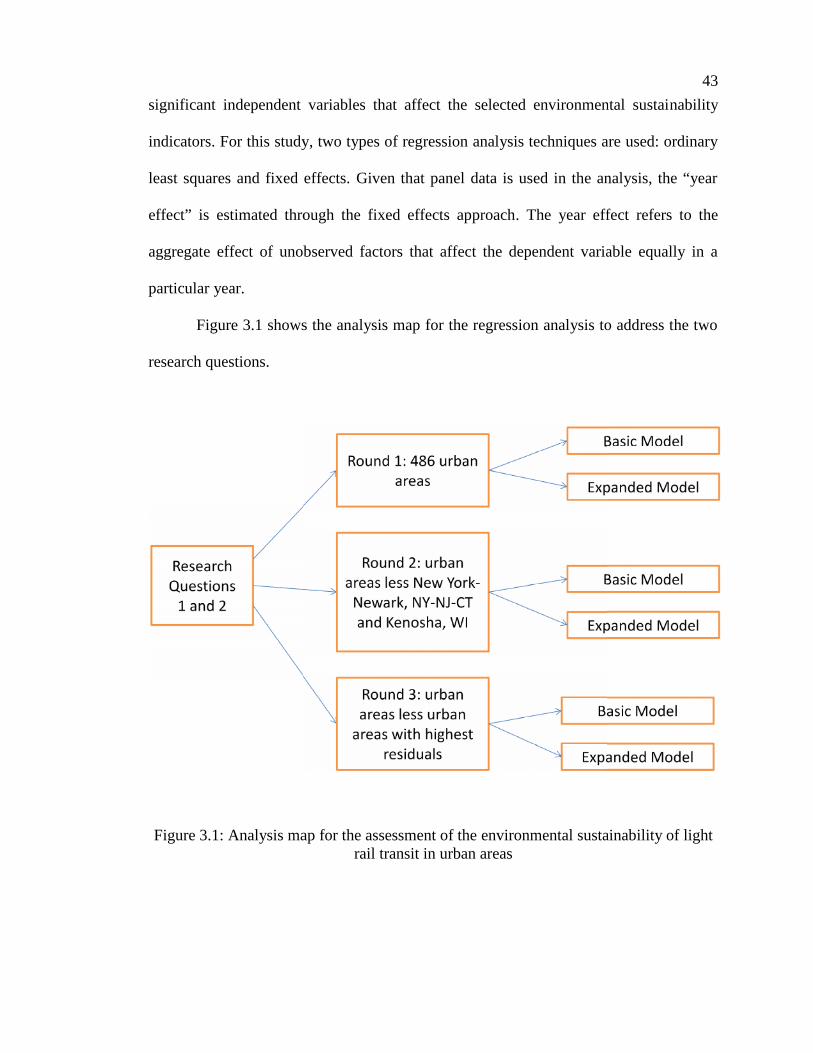
43
significant independent variables that affect the selected environmental sustainability
indicators. For this study, two types of regression analysis techniques are used: ordinary
least squares and fixed effects. Given that panel data is used in the analysis, the “year
effect” is estimated through the fixed effects approach. The year effect refers to the
aggregate effect of unobserved factors that affect the dependent variable equally in a
particular year.
Figure 3.1 shows the analysis map for the regression analysis to address the two
research questions.
Figure 3.1: Analysis map for the assessment of the environmental sustainability of lightrail transit in urban areas
44
Each research question will be addressed through a series of regression analysis.
Each question will be analyzed three rounds of regression analysis which covered three
types of datasets. The first round of regression analysis covers the dataset for all 486
urban areas included in the study. The second and the third rounds of regression analyses
cover additional regression analysis using dataset that removed two types of outliers.
Outliers in the dataset affect the results of the regression for the selected environmental
sustainability indicators, but removing them may strengthen and improve the regression
results. Two kinds of outliers are removed in the second and third datasets. The second
dataset removed urban areas with light rail transit that had the lowest and highest service
area populations. These urban areas refer to the New York-Newark, NY-NJ-CT urban
area, which has the largest service area population, and Kenosha, WI, which has the
lowest service area population. The third dataset comprises the urban areas less the
urban areas with the highest residuals from the results of the first round of regression
analysis. Among all urban areas, in the basic model, Phoenix-Mesa, AZ has the highest
residuals for air quality index, while Blacksburg, VA has the highest residuals for energy
intensity and CO2 intensity. Hilton Head Island, SC has the highest residuals for energy
consumption per capita and CO2 emissions per capita. These three urban areas were
removed from the dataset for the third round of regressions for the basic model. For the
expanded model, Phoenix-Mesa, AZ and Blacksburg, VA have the highest residuals for
air quality index, and for energy intensity and CO2 intensity, respectively. Highest
residuals for energy consumption per capita and CO2 emissions per capita are both from
the Boston, MA-NH-RI urban area. The three urban areas were removed from the
dataset for the expanded model of the third round of regressions.
45
All three types of dataset are analyzed through three rounds of regression. Each
round of regression is assessed through two types of models: basic and expanded
models. The model with the highest variances explained by the independent variables
(the model with the highest R-square) will be used for an impact analysis to demonstrate
how the actual values and predicted values change when some of the variables and
characteristics change. Changes that are tested in this study include:
1) Change in the number of urban areas with light rail presence based on size of
the urban areas; and
2) Change in level of light rail ridership.
The classification for the size of the urban areas is based on the urban area classification
used by the National Transit Database, as follows:
a) Small size urban areas – urban areas with population less than 200,000;
b) Medium size urban areas – urban areas with population greater than 200,000;
c) large size urban areas – urban areas with population greater than 1 million.
For changes in light rail transit ridership, a 25 percent, 50 percent, 75 percent and 100
percent increase from the actual light rail ridership is assumed. The average actual and
the average predicted values for each selected environmental sustainability indicators are
compared with the average predicted values for changes in light rail presence in urban
areas and light rail ridership. The impact analysis will generate additional explanations
of the relationship between significant independent variables and selected environmental
sustainability indicators.
46
Model Specifications
The regression analysis for each selected environmental sustainability indicator
will be presented in two models: basic or expanded, as described in the research design.
Each of the selected environmental sustainability indicators serves as dependent
variables that represent the outcome for the analysis. The first part of the analysis
includes analysis for all urban areas, while the second part includes analysis of urban
areas that have light rail. The model specifications for the analysis are listed as follows:
A. For All Urban Areas, 2000-2011, for each dependent variable (y):
1. Basic Model:
yit = f(year, lrt, hrt, crt, interaction terms) (Equation 3.2)
where y refers to the selected environmental sustainability indicator, such as a) air
quality index, b) energy intensity, c) energy consumption per capita, d) CO2 intensity
and e) CO2 emissions per capita; year refers to year effects; lrt refers to light rail
presence, hrt refers to heavy rail presence, crt, refers to commuter rail presence, and
interaction terms refer to combinations of light rail, heavy rail and commuter rail in
urban areas, such as a) light rail and commuter rail presence, b) light rail and heavy rail
presence, c) heavy rail and commuter rail presence, and d) light rail, heavy rail, and
commuter rail presence.
2. Expanded Model:
yit = f(year, lrt, hrt, crt, interaction terms, urban area characteristics,public transit characteristics)
(Equation 3.3)
where y refers to the selected environmental sustainability indicator, such as a) air
quality index, b) energy intensity, c) energy consumption per capita, d) CO2 intensity
and e) CO2 emissions per capita; year refers to year effects; lrt refers to light rail
47
presence, hrt refers to heavy rail presence, crt, refers to commuter rail presence, and
interaction terms refer to combinations of light rail, heavy rail and commuter rail in
urban areas, such as a) light rail and commuter rail presence, b) light rail and heavy rail
presence, c) heavy rail and commuter rail presence, and d) light rail, heavy rail, and
commuter rail presence; urban area characteristics refer to the following: a) population
density, b) housing density, and c) employment establishment density, and public transit
characteristics refer to the following: a) ridership, b) directional route miles, c)
operating expenses, and d) vehicles operating at maximum service.
B. For Urban Areas, 2000-2011, for each dependent variable (Y):
1. Basic Model
yit = f(year, lrt characteristics) (Equation 3.4)
where y refers to the selected environmental sustainability indicator, such as a) air
quality index, b) energy intensity, c) energy consumption per capita, d) CO2 intensity
and e) CO2 emissions per capita; year refers to year effects; lrt characteristics refer to
the following variables: a) light rail transit ridership; b) light rail transit directional route
miles; c) light rail transit operating expenses; d) light rail transit vehicles operated at
maximum service; e) light rail transit passenger miles; f) light rail transit energy
consumption, and g) light rail transit CO2 emissions.
2. Expanded Model
yit = f(year, lrt characteristics, urban area characteristics,public transit characteristics)
(Equation 3.5)
where y refers to the selected environmental sustainability indicator, such as a) air
quality index, b) energy intensity, c) energy consumption per capita, d) CO2 intensity
and e) CO2 emissions per capita; year refers to year effects; lrt characteristics refer to
48
the following variables: a) light rail transit ridership; b) light rail transit directional route
miles; c) light rail transit operating expenses; d) light rail transit vehicles operated at
maximum service; e) light rail transit passenger miles; f) light rail transit energy
consumption, and g) light rail transit CO2 emissions; urban area characteristics refer to
the following: a) population density, b) housing density, and c) employment
establishment density, and public transit characteristics refer to the following: a)
ridership, b) directional route miles, c) operating expenses, and d) vehicles operating at
maximum service.
Variables
The variables that will be used in the study are described the following list:
• Environmental sustainability indicators – air quality, energy consumption and
greenhouse gas emissions
• Light rail transit presence – whether or not light rail is present in the area
• Other forms of rail transit presence – commuter rail and heavy rail – whether or
not rail transit is present in the area
• Urban area characteristics – population, housing units, employment
establishments, and land area
• Light rail characteristics – ridership, operating expenses, directional route miles,
number of vehicles at maximum service, energy consumption, carbon dioxide
emissions
• Public transit characteristics - ridership, operating expenses, directional route
miles, and number of vehicles at maximum service.
49
The dependent variables for this study are the environmental sustainability
indicators – measured as air quality, energy consumption and greenhouse gas emissions.
The dependent variable is the observed outcome for this study and the variable that is
predicted based on the behavior of various determinants. The dependent variable for
minimizing pollution is the air quality index. The dependent variables for energy
consumption are energy intensity (which is the level of energy consumption (in British
thermal units) per passenger miles traveled) and energy consumption per capita (energy
consumption per population). The dependent variables for greenhouse gas emissions are
carbon dioxide emissions intensity (which is the level of carbon dioxide in an urban area
per output passenger miles traveled), and carbon dioxide emissions per capita (which is
the level of carbon dioxide in the urban area per population).
The independent variables for this study are the light rail transit and other forms
of rail transit presence in the urban area, the urban area characteristics and the selected
light rail operations and performance indicators. Light rail presence is measured as a
dichotomous ordinal data, either yes (1) or no (0), if light rail is present in the urban
area. Commuter rail and heavy rail presence is also included measured as dichotomous
ordinal data, either yes (1) or no (0), if commuter rail or heavy rail is present in the urban
area. To include urban areas that have combinations of rail transit systems, interaction
terms are created. Interaction terms for urban areas that have light rail, commuter rail,
heavy rail, or a combination of all rail systems is considered in the analysis. Urban area
characteristics in the analysis also include population density (number of people per area
square mile), housing density (number of housing units per area square mile) and
employment establishment density (number of employment establishments per area
50
square mile). The context for including urban densities takes into consideration how
urban form matters in the analysis – the more dense an area, how do urban areas with or
without light rail affect environmental sustainability. Lastly, public transit characteristics
included as independent variables are as follows:
a) total ridership in the area – regardless of what type of public transit mode
people use,
b) total directional route miles for all transit modes,
c) total operating expenses for public transit, and
d) Total number of vehicles used at maximum service – in the case of rail, this
refers to the number of rail passenger cars used at maximum service.
Light rail transit characteristics are also included in the study, as follows:
a) ridership for light rail,
b) directional route miles for light rail,
c) operating expenses for light rail,
d) the number of light rail vehicles used at maximum service,
e) light rail energy consumption, and
f) Light rail carbon dioxide emissions per urban area.
For the regressions analysis, the urban area characteristics and the public transit
characteristics are used as control variables. Key variable of interest for the first research
question is light rail presence in urban areas. For the second research question,
significant variables emerge from the analysis and the direction of the relationship of
these variables to the selected environmental sustainability indicators will be discussed.
51
Data Collection, Preparation and Analysis
The dataset used for this study is a panel dataset drawn from 486 urbanized areas
in 50 U.S. states, including District of Columbia. The panel data contains observations
from 12 years, from 2000 to 2011. The data used in this study is collected from:
a) the National Transit Database, compiled by the Federal Transit
Administration,
b) Air Quality Reports from the Environmental Protection Agency,
c) Annual databases from the Energy Information Administration, and
d) Data from the U.S. Census Bureau.
The methods for collecting and preparing the data for analysis for each variable are
explained as follows:
1. Air quality index
Data for air quality index is collected from the air quality index report produced
by the EPA. The median air quality index was used in the study, which represents half of
the daily air quality index values during the year that were less than or equal to the
median value of the index. Table 3.1 presents the range of air quality index values and
the levels of health concerns. The annual summary information for air quality index is
generated from the air quality data website of the EPA:
http://www.epa.gov/airdata/ad_rep_aqi.html.
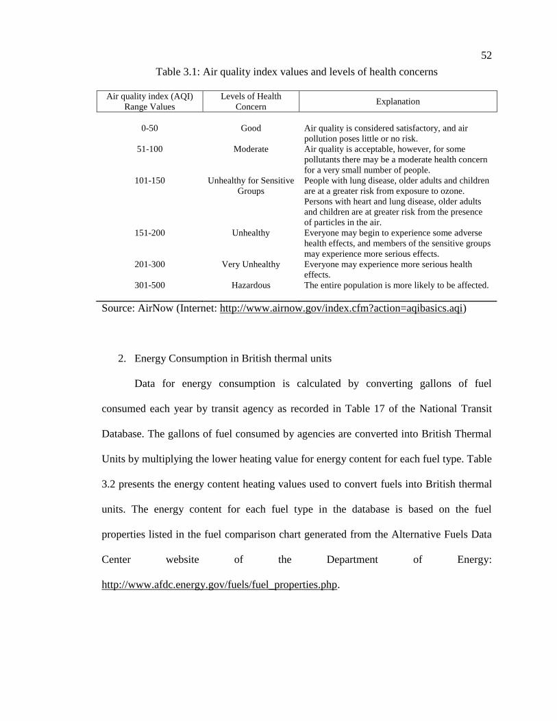
52
Table 3.1: Air quality index values and levels of health concerns
Air quality index (AQI)Range Values
Levels of HealthConcern
Explanation
0-50 Good Air quality is considered satisfactory, and airpollution poses little or no risk.
51-100 Moderate Air quality is acceptable, however, for somepollutants there may be a moderate health concernfor a very small number of people.
101-150 Unhealthy for SensitiveGroups
People with lung disease, older adults and childrenare at a greater risk from exposure to ozone.Persons with heart and lung disease, older adultsand children are at greater risk from the presenceof particles in the air.
151-200 Unhealthy Everyone may begin to experience some adversehealth effects, and members of the sensitive groupsmay experience more serious effects.
201-300 Very Unhealthy Everyone may experience more serious healtheffects.
301-500 Hazardous The entire population is more likely to be affected.
Source: AirNow (Internet: http://www.airnow.gov/index.cfm?action=aqibasics.aqi)
2. Energy Consumption in British thermal units
Data for energy consumption is calculated by converting gallons of fuel
consumed each year by transit agency as recorded in Table 17 of the National Transit
Database. The gallons of fuel consumed by agencies are converted into British Thermal
Units by multiplying the lower heating value for energy content for each fuel type. Table
3.2 presents the energy content heating values used to convert fuels into British thermal
units. The energy content for each fuel type in the database is based on the fuel
properties listed in the fuel comparison chart generated from the Alternative Fuels Data
Center website of the Department of Energy:
http://www.afdc.energy.gov/fuels/fuel_properties.php.
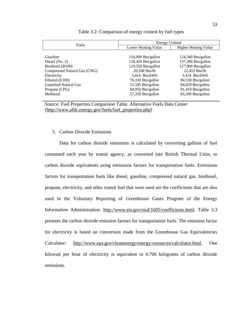
53
Table 3.2: Comparison of energy content by fuel types
FuelsEnergy Content
Lower Heating Value Higher Heating Value
Gasoline 116,090 Btu/gallon 124,340 Btu/gallonDiesel (No. 2) 128,450 Btu/gallon 137,380 Btu/gallonBiodiesel (B100) 119,550 Btu/gallon 127,960 Btu/gallonCompressed Natural Gas (CNG) 20,268 Btu/lb 22,453 Btu/lbElectricity 3,414 Btu/kWh 3,414 Btu/kWhEthanol (E100) 76,330 Btu/gallon 84,530 Btu/gallonLiquefied Natural Gas 51,585 Btu/gallon 84,820 Btu/gallonPropane (LPG) 84,950 Btu/gallon 91,410 Btu/gallonMethanol 57,250 Btu/gallon 65,200 Btu/gallon
Source: Fuel Properties Comparison Table. Alternative Fuels Data Center(http://www.afdc.energy.gov/fuels/fuel_properties.php)
3. Carbon Dioxide Emissions
Data for carbon dioxide emissions is calculated by converting gallons of fuel
consumed each year by transit agency, as converted into British Thermal Units, to
carbon dioxide equivalents using emissions factors for transportation fuels. Emissions
factors for transportation fuels like diesel, gasoline, compressed natural gas, biodiesel,
propane, electricity, and other transit fuel that were used are the coefficients that are also
used in the Voluntary Reporting of Greenhouse Gases Program of the Energy
Information Administration: http://www.eia.gov/oiaf/1605/coefficients.html. Table 3.3
presents the carbon dioxide emission factors for transportation fuels. The emission factor
for electricity is based on conversion made from the Greenhouse Gas Equivalencies
Calculator: http://www.epa.gov/cleanenergy/energy-resources/calculator.html. One
kilowatt per hour of electricity is equivalent to 0.706 kilograms of carbon dioxide
emissions.
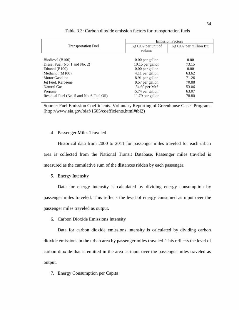
54
Table 3.3: Carbon dioxide emission factors for transportation fuels
Transportation FuelEmission Factors
Kg CO2 per unit ofvolume
Kg CO2 per million Btu
Biodiesel (B100) 0.00 per gallon 0.00Diesel Fuel (No. 1 and No. 2) 10.15 per gallon 73.15Ethanol (E100) 0.00 per gallon 0.00Methanol (M100) 4.11 per gallon 63.62Motor Gasoline 8.91 per gallon 71.26Jet Fuel, Kerosene 9.57 per gallon 70.88Natural Gas 54.60 per Mcf 53.06Propane 5.74 per gallon 63.07Residual Fuel (No. 5 and No. 6 Fuel Oil) 11.79 per gallon 78.80
Source: Fuel Emission Coefficients. Voluntary Reporting of Greenhouse Gases Program(http://www.eia.gov/oiaf/1605/coefficients.html#tbl2)
4. Passenger Miles Traveled
Historical data from 2000 to 2011 for passenger miles traveled for each urban
area is collected from the National Transit Database. Passenger miles traveled is
measured as the cumulative sum of the distances ridden by each passenger.
5. Energy Intensity
Data for energy intensity is calculated by dividing energy consumption by
passenger miles traveled. This reflects the level of energy consumed as input over the
passenger miles traveled as output.
6. Carbon Dioxide Emissions Intensity
Data for carbon dioxide emissions intensity is calculated by dividing carbon
dioxide emissions in the urban area by passenger miles traveled. This reflects the level of
carbon dioxide that is emitted in the area as input over the passenger miles traveled as
output.
7. Energy Consumption per Capita
55
Data for energy consumption per capita is calculated by dividing energy
consumption over total population of the urban area.
8. Carbon Dioxide Emissions per Capita
Data for carbon dioxide emissions per capita is calculated by dividing carbon
dioxide emissions in the urban area over total population of the urban area.
9. Population Estimates
Population data for each urban area is available for census years 2000 and 2010.
Population estimates are calculated using a growth rate method, wherein growth
increments are spread throughout the years from 2000 to 2011 using the population
growth rate.
10. Land Area Estimates
Land area data for each urban area is available for census years 2000 and 2010.
Land area estimates are calculated using a growth rate method, wherein growth
increments are spread throughout the years from 2000 to 2011 using the population
growth rate.
11. Housing Units Estimates
Housing units’ data for each urban area is available for census years 2000 and
2010. Housing units’ estimates are calculated using a growth rate method, wherein
growth increments are spread throughout the years from 2000 to 2011 using the
population growth rate.
12. Employment Establishments Estimates
Data for the total number of employment establishments is available from the
County and Metropolitan Statistical Area Business Patterns database under the North
56
American Industry Classification System (NAICS). Data for years 2000 to 2010 was
generated from the Censtats website: http://censtats.census.gov/cgi-
bin/msanaic/msasect.pl) while data for 2011 is estimated, using data from 2010 levels,
assuming that there are no changes in the number of establishments in the area from
2010 to 2011.
13. Population Density
Population density for each urban area is calculated by dividing the population of
the urban area with the land area in square miles.
14. Housing Density
Housing density for each urban area is calculated by dividing the total number of
housing units in the urban area with the land area in square miles.
15. Employment Establishment Density
Employment establishment density for each urban area is calculated by dividing
the total number of employment establishment in the urban area with the land area in
square miles.
16. Total Ridership
Historical data from 2000 to 2011 for ridership for each urban area is collected
from the National Transit Database. This indicator is represented by unlinked passenger
trips (UPT), which is defined as the number of passengers who board public
transportation vehicles. Passengers are counted each time they board vehicles no matter
how many vehicles they use to travel from their origin to their destination.
17. Total Directional Route Miles for Each Urban Area
57
Historical data from 2000 to 2011 for directional route miles for each urban area
is collected from the National Transit Database. Directional route miles are the mileage
in each direction over which public transportation vehicles travel while in revenue
service. Directional route miles are a measure of the route path over a facility or
roadway and are computed with regard to the direction of the service, but without regard
to the number of traffic lanes or rail tracks existing in the right-of-way. The directional
route miles do not include the staging or storage areas at the beginning or the end of a
route.
18. Total Operating Expenses for Transit Modes
Historical data from 2000 to 2011 for operational expenses for each urban area is
collected from the National Transit Database. The operating expenses are the expenses
associated with the operation of the transit agency.
19. Total Vehicles Operated at Maximum Service
Historical data from 2000 to 2011 for the total vehicles operated at maximum
service directional route miles for each urban area is collected from the National Transit
Database. The vehicles operated at maximum service indicator are the number of
revenue vehicles operated to meet the annual maximum service requirement. This is the
revenue vehicle count during the peak season of the year, on the week day that
maximum service is provided. Vehicles operated in maximum service exclude atypical
days or one-time special events.
20. Light Rail Ridership
Historical data from 2000 to 2011 for the light rail transit ridership for each
urban area is collected from the National Transit Database.
58
21. Light Rail Directional Route Miles for Each Urban Area
Historical data from 2000 to 2011 for the light rail transit directional route miles
for each urban area is collected from the National Transit Database.
22. Light Rail Operating Expenses
Historical data from 2000 to 2011 for the light rail transit operating expenses for
each urban area is collected from the National Transit Database.
23. Light Rail Vehicles Operated at Maximum Service
Historical data from 2000 to 2011 for the light rail passenger vehicles operated at
maximum service is collected from the National Transit Database.
24. Light Rail Presence
Data for light rail presence included in the study is based on operating expenses
data for transit modes from the National Transit Database. Data used in the analysis is
converted to ordinal data, wherein the numbers 1 and 0 are used to indicate whether light
rail is available in the urban area.
25. Commuter Rail Presence
Data for commuter rail presence included in the study is based on operating
expenses data for transit modes from the National Transit Database. Data used in the
analysis is converted to ordinal data, wherein the numbers 1 and 0 are used to indicate
whether commuter rail is available in the urban area.
26. Heavy Rail Presence
Data for heavy rail presence included in the study is based on operating expenses
data for transit modes from the National Transit Database. Data used in the analysis is
59
converted to ordinal data, wherein the numbers 1 and 0 are used to indicate whether light
rail is available in the urban area.
27. Bus System Presence
Data for bus system presence included in the study is based on operating
expenses data for transit modes from the National Transit Database. Data used in the
analysis is converted to ordinal data, wherein the numbers 1 and 0 are used to indicate
whether bus systems rail is available in the urban area.
28. Light Rail Energy Consumption
Data for light rail energy consumption is calculated based on lower energy
content for electricity multiplied by the number of kilowatt hours used for operating light
rail services. The fuel conversion factor of the energy from electric propulsion is based
on the energy content values in Table 3-2.
29. Light Rail Carbon Dioxide Emissions
Data for light rail carbon dioxide emissions is calculated based on the emission
factor for electricity. The emission factor for electricity is based on conversion made
from the Greenhouse Gas Equivalencies Calculator of the EPA:
http://www.epa.gov/cleanenergy/energy-resources/calculator.html. One kilowatt per
hour of electricity is equivalent to 0.706 kilograms of carbon dioxide emissions.
Chapter Summary
This chapter presented a detailed description of the method of analysis, the
research design and the data used for conducting the statistical analysis, regression
analysis and the technical analysis to address the research questions.

60
The results of the analysis will be presented in the succeeding chapter. A
summary of the output tables will be presented for each round of regression analysis.
Supporting tables and detailed regression outputs will be presented in the Appendices
section of the study.
61
CHAPTER 4: PRESENTATION OF THE RESULTS OF ANALYSIS
The descriptive statistics for all variables used in the study as well as the
significant bivariate regression results and results of the series of multiple regression
analysis are presented in this chapter. Descriptive statistics on all variables used in this
analysis are presented in the first section. The second section presents the significant
bivariate regression results for all dependent variables and selected independent
variables. The bivariate regression shows the general direction by which each variable
affect the environmental sustainability indicators. The third section presents the results
of the series of regression analysis to address each of the research questions. The
regression analysis results are presented in two parts for each research question, and
include the discussion of the results for each round of regressions. The regressions with
the largest percentages of variances explained by independent variables will be used for
an impact analysis for changes in light rail presence in urban areas and for changes in
ridership. The results of the impact analysis are also presented in this chapter.
A summary of the regression analysis for both OLS and fixed effects approaches
is presented in Appendix B. For each analysis result, key measures to consider are the R-
square and the F-ratio. The R-square measures the proportion of the variation explained
by the model. The model fits perfectly is the value of the R-square is equal to 1. An R-
square closer to 0, on the other hand, indicates that the fit predicts that the model is no
better than the overall response mean. In other words, the model with a lower R-square
62
is not a good predictor model for environmental sustainability. The F-ratio, on the other
hand, evaluates the effectiveness of the model, and is presented in the analysis of
variance. If the probability associated with the F-ratio is small, then the model is
considered a better statistical fit for the data used in the study. The observed significance
probability (p-value) of 0.05 or less is often considered as evidence of a regression
effect. In other words, estimates must have p-values less than 0.05 to be considered as
significant estimates of factors for the model.
Descriptive Statistics
Table 4.1 presents the summary of the descriptive statistics for selected
environmental sustainability indicators used in the analysis.
For selected environmental sustainability indicators, average air quality index for
all data used in all urban areas is 41, which is within the range of 0-50, where air quality
conditions are described as “good” (Table 3.1). Average energy intensity for all data for
urban areas included in this study is 7,582 BTU per passenger mile, while average
energy consumption per capita is 305,240 BTU. Average carbon dioxide emissions
intensity is 0.52 kilograms of CO2 per passenger mile, while average CO2 emission per
capita is 20 kilograms of CO2.
Average energy consumption for urban areas is 382.6 billion BTUs, while
average CO2 emission for urban areas is 21.7 million kilograms of carbon dioxide.
Average passenger miles traveled in urban areas is 144.3 million miles. On the average,
population density is about 2,110 people per area square mile, while there are about
1,271 houses per area square mile. In urban areas, there are about 80 employment
establishments per are square mile.
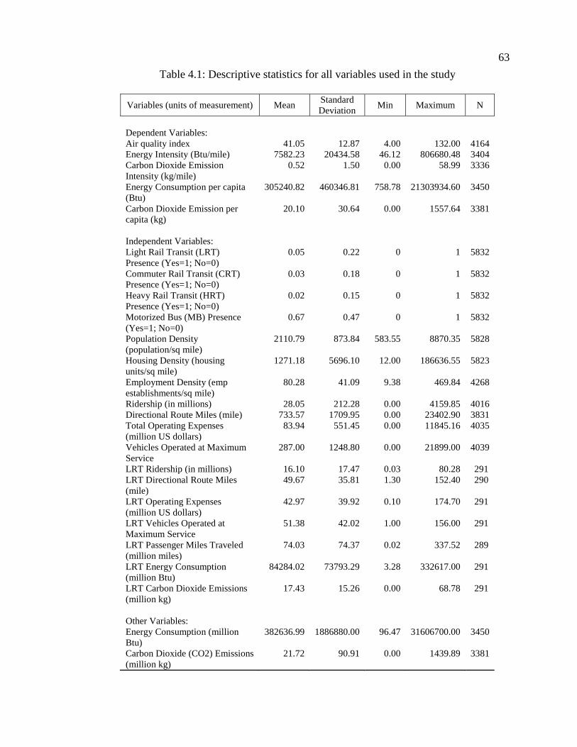
63
Table 4.1: Descriptive statistics for all variables used in the study
Variables (units of measurement) MeanStandardDeviation
Min Maximum N
Dependent Variables:Air quality index 41.05 12.87 4.00 132.00 4164Energy Intensity (Btu/mile) 7582.23 20434.58 46.12 806680.48 3404Carbon Dioxide EmissionIntensity (kg/mile)
0.52 1.50 0.00 58.99 3336
Energy Consumption per capita(Btu)
305240.82 460346.81 758.78 21303934.60 3450
Carbon Dioxide Emission percapita (kg)
20.10 30.64 0.00 1557.64 3381
Independent Variables:Light Rail Transit (LRT)Presence (Yes=1; No=0)
0.05 0.22 0 1 5832
Commuter Rail Transit (CRT)Presence (Yes=1; No=0)
0.03 0.18 0 1 5832
Heavy Rail Transit (HRT)Presence (Yes=1; No=0)
0.02 0.15 0 1 5832
Motorized Bus (MB) Presence(Yes=1; No=0)
0.67 0.47 0 1 5832
Population Density(population/sq mile)
2110.79 873.84 583.55 8870.35 5828
Housing Density (housingunits/sq mile)
1271.18 5696.10 12.00 186636.55 5823
Employment Density (empestablishments/sq mile)
80.28 41.09 9.38 469.84 4268
Ridership (in millions) 28.05 212.28 0.00 4159.85 4016Directional Route Miles (mile) 733.57 1709.95 0.00 23402.90 3831Total Operating Expenses(million US dollars)
83.94 551.45 0.00 11845.16 4035
Vehicles Operated at MaximumService
287.00 1248.80 0.00 21899.00 4039
LRT Ridership (in millions) 16.10 17.47 0.03 80.28 291LRT Directional Route Miles(mile)
49.67 35.81 1.30 152.40 290
LRT Operating Expenses(million US dollars)
42.97 39.92 0.10 174.70 291
LRT Vehicles Operated atMaximum Service
51.38 42.02 1.00 156.00 291
LRT Passenger Miles Traveled(million miles)
74.03 74.37 0.02 337.52 289
LRT Energy Consumption(million Btu)
84284.02 73793.29 3.28 332617.00 291
LRT Carbon Dioxide Emissions(million kg)
17.43 15.26 0.00 68.78 291
Other Variables:Energy Consumption (millionBtu)
382636.99 1886880.00 96.47 31606700.00 3450
Carbon Dioxide (CO2) Emissions(million kg)
21.72 90.91 0.00 1439.89 3381
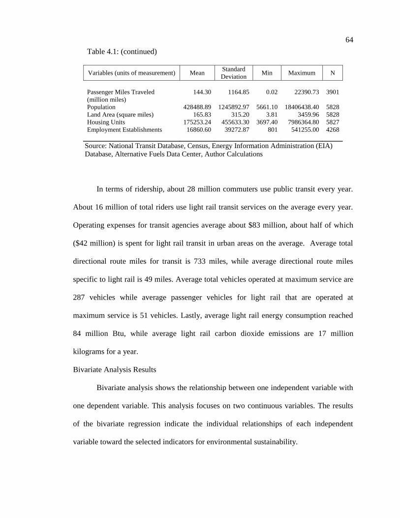
64
Table 4.1: (continued)
Variables (units of measurement) MeanStandardDeviation
Min Maximum N
Passenger Miles Traveled(million miles)
144.30 1164.85 0.02 22390.73 3901
Population 428488.89 1245892.97 5661.10 18406438.40 5828Land Area (square miles) 165.83 315.20 3.81 3459.96 5828Housing Units 175253.24 455633.30 3697.40 7986364.80 5827Employment Establishments 16860.60 39272.87 801 541255.00 4268
Source: National Transit Database, Census, Energy Information Administration (EIA)Database, Alternative Fuels Data Center, Author Calculations
In terms of ridership, about 28 million commuters use public transit every year.
About 16 million of total riders use light rail transit services on the average every year.
Operating expenses for transit agencies average about $83 million, about half of which
($42 million) is spent for light rail transit in urban areas on the average. Average total
directional route miles for transit is 733 miles, while average directional route miles
specific to light rail is 49 miles. Average total vehicles operated at maximum service are
287 vehicles while average passenger vehicles for light rail that are operated at
maximum service is 51 vehicles. Lastly, average light rail energy consumption reached
84 million Btu, while average light rail carbon dioxide emissions are 17 million
kilograms for a year.
Bivariate Analysis Results
Bivariate analysis shows the relationship between one independent variable with
one dependent variable. This analysis focuses on two continuous variables. The results
of the bivariate regression indicate the individual relationships of each independent
variable toward the selected indicators for environmental sustainability.
65
A summary of the results of the bivariate analysis is presented in Table 4-2.
Based on the results, light rail presence is a significant determinant for all the selected
environmental sustainability indicators, however, the models show low R-square values.
The models for air quality index, energy per capita and CO2 emissions per capita, show
9 percent, 5 percent and 3 percent of the variance in light rail presence respectively. For
energy intensity and CO2 intensity models, the R-square is less than one percent. This
means that only less than 1 percent of the variance is explained. For all the models, the
results indicate that the bivariate models for light rail presence and environmental
sustainability indicators are not good models for predicting environmental sustainability
in urban areas.
The bivariate analysis also indicates that the commuter rail presence, heavy rail
presence, population density, and housing density are not good predictors of all five
environmental sustainability indicators. Employment density, however, indicates that
good predictability for energy per capita and CO2 per capita. About 10 percent of the
variance in the models can be explained by employment density. The results also
indicate that ridership has a significant relationship with energy per capita. About 20
percent of the variance can be explained in the model between ridership and energy per
capita.
Directional route miles affect air quality index, energy per capita and CO2 per
capita. R-square values are 12 percent, 33 percent and 19 percent respectively. The
variance for energy per capital model has a larger R-square value, which means that
there is a larger chance of a better bivariate fit. Operating expenses and vehicles
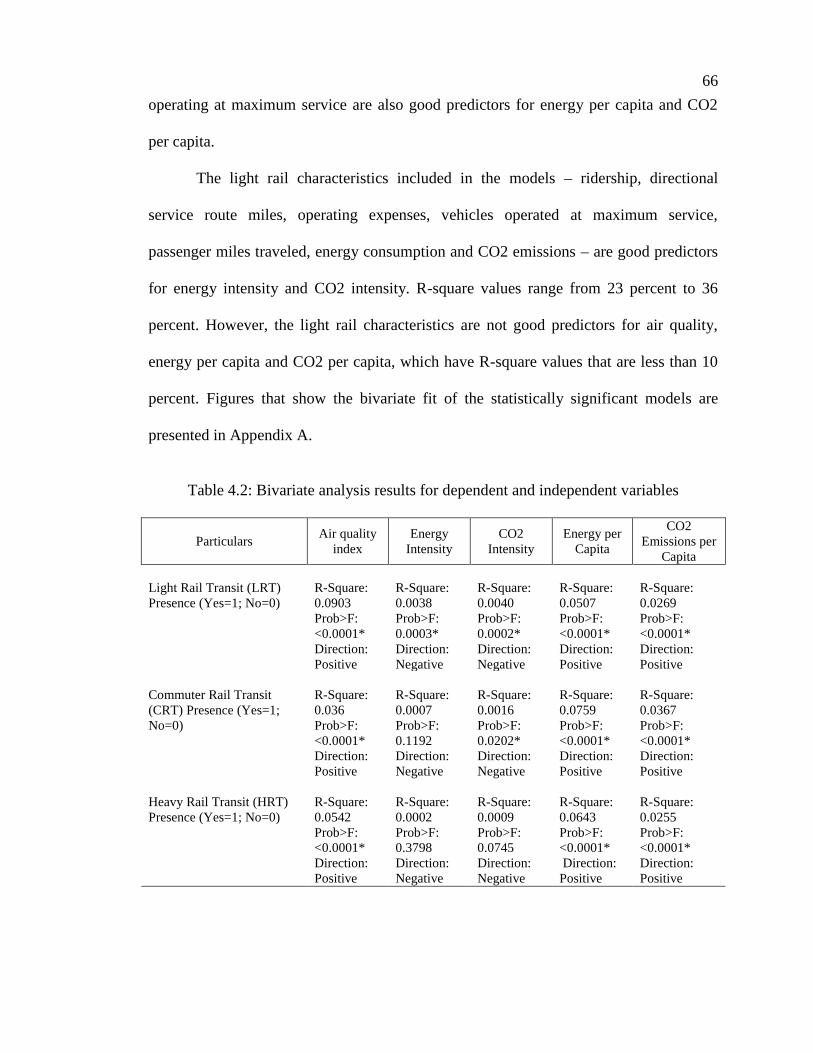
66
operating at maximum service are also good predictors for energy per capita and CO2
per capita.
The light rail characteristics included in the models – ridership, directional
service route miles, operating expenses, vehicles operated at maximum service,
passenger miles traveled, energy consumption and CO2 emissions – are good predictors
for energy intensity and CO2 intensity. R-square values range from 23 percent to 36
percent. However, the light rail characteristics are not good predictors for air quality,
energy per capita and CO2 per capita, which have R-square values that are less than 10
percent. Figures that show the bivariate fit of the statistically significant models are
presented in Appendix A.
Table 4.2: Bivariate analysis results for dependent and independent variables
ParticularsAir quality
indexEnergy
IntensityCO2
IntensityEnergy per
Capita
CO2Emissions per
Capita
Light Rail Transit (LRT)Presence (Yes=1; No=0)
R-Square:0.0903Prob>F:<0.0001*Direction:Positive
R-Square:0.0038Prob>F:0.0003*Direction:Negative
R-Square:0.0040Prob>F:0.0002*Direction:Negative
R-Square:0.0507Prob>F:<0.0001*Direction:Positive
R-Square:0.0269Prob>F:<0.0001*Direction:Positive
Commuter Rail Transit(CRT) Presence (Yes=1;No=0)
R-Square:0.036Prob>F:<0.0001*Direction:Positive
R-Square:0.0007Prob>F:0.1192Direction:Negative
R-Square:0.0016Prob>F:0.0202*Direction:Negative
R-Square:0.0759Prob>F:<0.0001*Direction:Positive
R-Square:0.0367Prob>F:<0.0001*Direction:Positive
Heavy Rail Transit (HRT)Presence (Yes=1; No=0)
R-Square:0.0542Prob>F:<0.0001*Direction:Positive
R-Square:0.0002Prob>F:0.3798Direction:Negative
R-Square:0.0009Prob>F:0.0745Direction:Negative
R-Square:0.0643Prob>F:<0.0001*Direction:
Positive
R-Square:0.0255Prob>F:<0.0001*Direction:Positive
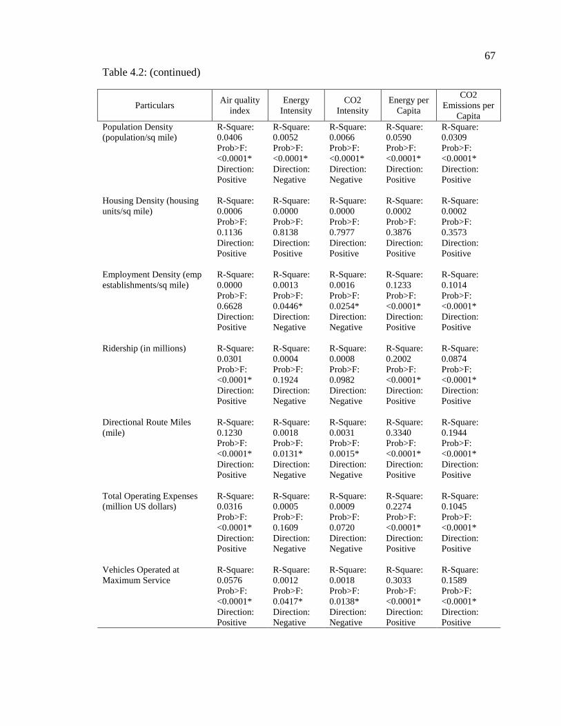
67
Table 4.2: (continued)
ParticularsAir quality
indexEnergy
IntensityCO2
IntensityEnergy per
Capita
CO2Emissions per
CapitaPopulation Density(population/sq mile)
R-Square:0.0406Prob>F:<0.0001*Direction:Positive
R-Square:0.0052Prob>F:<0.0001*Direction:Negative
R-Square:0.0066Prob>F:<0.0001*Direction:Negative
R-Square:0.0590Prob>F:<0.0001*Direction:Positive
R-Square:0.0309Prob>F:<0.0001*Direction:Positive
Housing Density (housingunits/sq mile)
R-Square:0.0006Prob>F:0.1136Direction:Positive
R-Square:0.0000Prob>F:0.8138Direction:Positive
R-Square:0.0000Prob>F:0.7977Direction:Positive
R-Square:0.0002Prob>F:0.3876Direction:Positive
R-Square:0.0002Prob>F:0.3573Direction:Positive
Employment Density (empestablishments/sq mile)
R-Square:0.0000Prob>F:0.6628Direction:Positive
R-Square:0.0013Prob>F:0.0446*Direction:Negative
R-Square:0.0016Prob>F:0.0254*Direction:Negative
R-Square:0.1233Prob>F:<0.0001*Direction:Positive
R-Square:0.1014Prob>F:<0.0001*Direction:Positive
Ridership (in millions) R-Square:0.0301Prob>F:<0.0001*Direction:Positive
R-Square:0.0004Prob>F:0.1924Direction:Negative
R-Square:0.0008Prob>F:0.0982Direction:Negative
R-Square:0.2002Prob>F:<0.0001*Direction:Positive
R-Square:0.0874Prob>F:<0.0001*Direction:Positive
Directional Route Miles(mile)
R-Square:0.1230Prob>F:<0.0001*Direction:Positive
R-Square:0.0018Prob>F:0.0131*Direction:Negative
R-Square:0.0031Prob>F:0.0015*Direction:Negative
R-Square:0.3340Prob>F:<0.0001*Direction:Positive
R-Square:0.1944Prob>F:<0.0001*Direction:Positive
Total Operating Expenses(million US dollars)
R-Square:0.0316Prob>F:<0.0001*Direction:Positive
R-Square:0.0005Prob>F:0.1609Direction:Negative
R-Square:0.0009Prob>F:0.0720Direction:Negative
R-Square:0.2274Prob>F:<0.0001*Direction:Positive
R-Square:0.1045Prob>F:<0.0001*Direction:Positive
Vehicles Operated atMaximum Service
R-Square:0.0576Prob>F:<0.0001*Direction:Positive
R-Square:0.0012Prob>F:0.0417*Direction:Negative
R-Square:0.0018Prob>F:0.0138*Direction:Negative
R-Square:0.3033Prob>F:<0.0001*Direction:Positive
R-Square:0.1589Prob>F:<0.0001*Direction:Positive
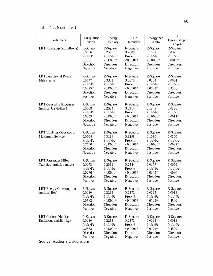
68
Table 4.2: (continued)
ParticularsAir quality
indexEnergy
IntensityCO2
IntensityEnergy per
Capita
CO2Emissions per
CapitaLRT Ridership (in millions) R-Square:
0.0036Prob>F:0.3151Direction:Negative
R-Square:0.2515Prob>F:<0.0001*Direction:Negative
R-Square:0.2600Prob>F:<0.0001*Direction:Negative
R-Square:0.1071Prob>F:<0.0001*Direction:Positive
R-Square:0.0370Prob>F:0.0010*Direction:Positive
LRT Directional RouteMiles (mile)
R-Square:0.0147Prob>F:0.0425*Direction:Positive
R-Square:0.3351Prob>F:<0.0001*Direction:Negative
R-Square:0.3670Prob>F:<0.0001*Direction:Negative
R-Square:0.0284Prob>F:0.0039*Direction:Positive
R-Square:0.0001Prob>F:0.8386Direction:Positive
LRT Operating Expenses(million US dollars)
R-Square:0.0008Prob>F:0.6353Direction:Negative
R-Square:0.2654Prob>F:<0.0001*Direction:Negative
R-Square:0.2914Prob>F:<0.0001*Direction:Negative
R-Square:0.1349Prob>F:<0.0001*Direction:Positive
R-Square:0.0360Prob>F:0.0011*Direction:Positive
LRT Vehicles Operated atMaximum Service
R-Square:0.0004Prob>F:0.7140Direction:Negative
R-Square:0.3134Prob>F:<0.0001*Direction:Negative
R-Square:0.3298Prob>F:<0.0001*Direction:Negative
R-Square:0.1080Prob>F:<0.0001*Direction:Positive
R-Square:0.0306Prob>F:0.0027*Direction:Positive
LRT Passenger MilesTraveled (million miles)
R-Square:0.0173Prob>F:0.0276*Direction:Positive
R-Square:0.2331Prob>F:<0.0001*Direction:Negative
R-Square:0.2544Prob>F:<0.0001*Direction:Negative
R-Square:0.0177Prob>F:0.0234*Direction:Positive
R-Square:0.0009Prob>F:0.6094Direction:Positive
LRT Energy Consumption(million Btu)
R-Square:0.0130Prob>F:0.0563Direction:Positive
R-Square:0.2238Prob>F:<0.0001*Direction:Negative
R-Square:0.2572Prob>F:<0.0001*Direction:Negative
R-Square:0.0215Prob>F:0.0122*Direction:Positive
R-Square:0.0018Prob>F:0.4592Direction:Positive
LRT Carbon DioxideEmissions (million kg)
R-Square:0.0130Prob>F:0.0563Direction:Positive
R-Square:0.2238Prob>F:<0.0001*Direction:Negative
R-Square:0.2572Prob>F:<0.0001*Direction:Negative
R-Square:0.0215Prob>F:0.0122*Direction:Positive
R-Square:0.0018Prob>F:0.4592Direction:Positive
Source: Author’s Calculations
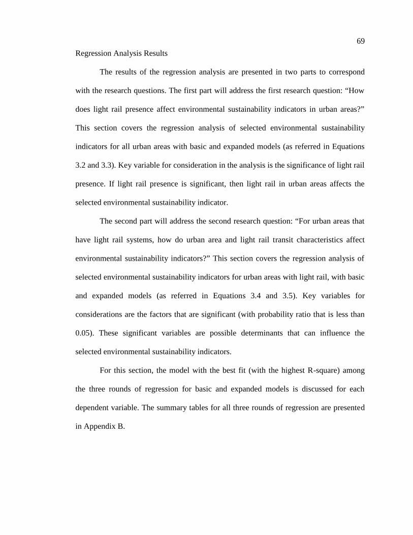
69
Regression Analysis Results
The results of the regression analysis are presented in two parts to correspond
with the research questions. The first part will address the first research question: “How
does light rail presence affect environmental sustainability indicators in urban areas?”
This section covers the regression analysis of selected environmental sustainability
indicators for all urban areas with basic and expanded models (as referred in Equations
3.2 and 3.3). Key variable for consideration in the analysis is the significance of light rail
presence. If light rail presence is significant, then light rail in urban areas affects the
selected environmental sustainability indicator.
The second part will address the second research question: “For urban areas that
have light rail systems, how do urban area and light rail transit characteristics affect
environmental sustainability indicators?” This section covers the regression analysis of
selected environmental sustainability indicators for urban areas with light rail, with basic
and expanded models (as referred in Equations 3.4 and 3.5). Key variables for
considerations are the factors that are significant (with probability ratio that is less than
0.05). These significant variables are possible determinants that can influence the
selected environmental sustainability indicators.
For this section, the model with the best fit (with the highest R-square) among
the three rounds of regression for basic and expanded models is discussed for each
dependent variable. The summary tables for all three rounds of regression are presented
in Appendix B.
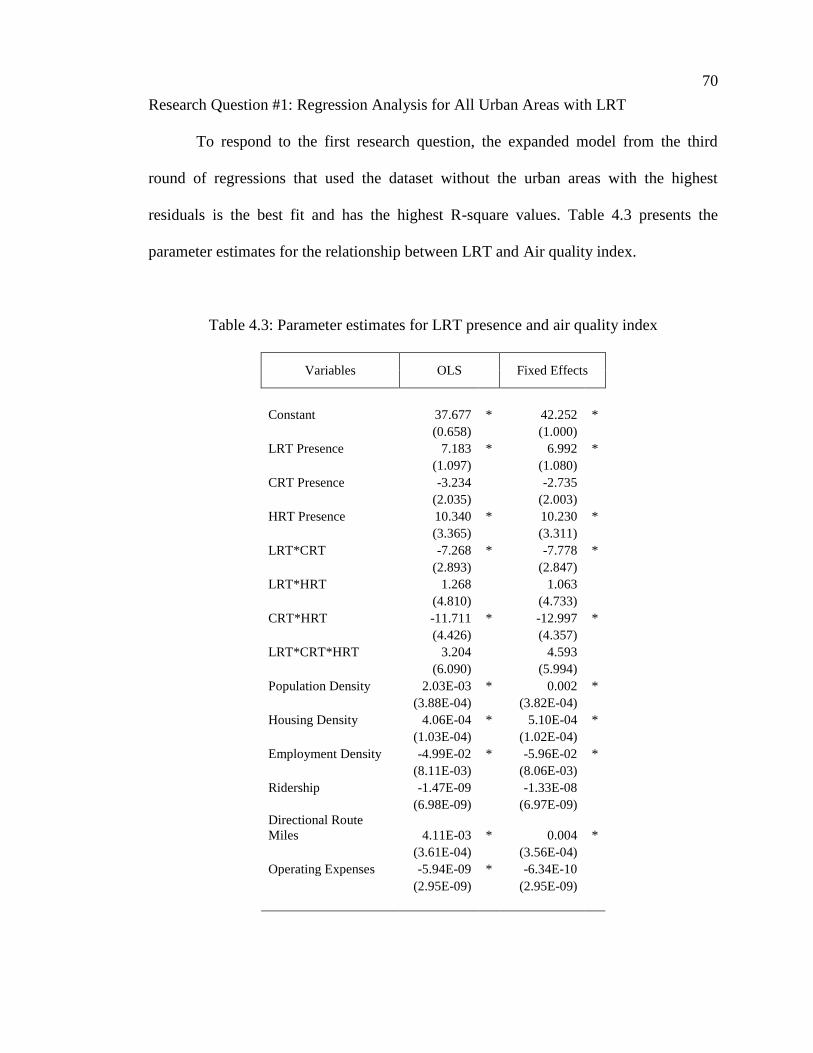
70
Research Question #1: Regression Analysis for All Urban Areas with LRT
To respond to the first research question, the expanded model from the third
round of regressions that used the dataset without the urban areas with the highest
residuals is the best fit and has the highest R-square values. Table 4.3 presents the
parameter estimates for the relationship between LRT and Air quality index.
Table 4.3: Parameter estimates for LRT presence and air quality index
Variables OLS Fixed Effects
Constant 37.677 * 42.252 *(0.658) (1.000)
LRT Presence 7.183 * 6.992 *(1.097) (1.080)
CRT Presence -3.234 -2.735(2.035) (2.003)
HRT Presence 10.340 * 10.230 *(3.365) (3.311)
LRT*CRT -7.268 * -7.778 *(2.893) (2.847)
LRT*HRT 1.268 1.063(4.810) (4.733)
CRT*HRT -11.711 * -12.997 *(4.426) (4.357)
LRT*CRT*HRT 3.204 4.593(6.090) (5.994)
Population Density 2.03E-03 * 0.002 *(3.88E-04) (3.82E-04)
Housing Density 4.06E-04 * 5.10E-04 *(1.03E-04) (1.02E-04)
Employment Density -4.99E-02 * -5.96E-02 *(8.11E-03) (8.06E-03)
Ridership -1.47E-09 -1.33E-08(6.98E-09) (6.97E-09)
Directional RouteMiles 4.11E-03 * 0.004 *
(3.61E-04) (3.56E-04)Operating Expenses -5.94E-09 * -6.34E-10
(2.95E-09) (2.95E-09)
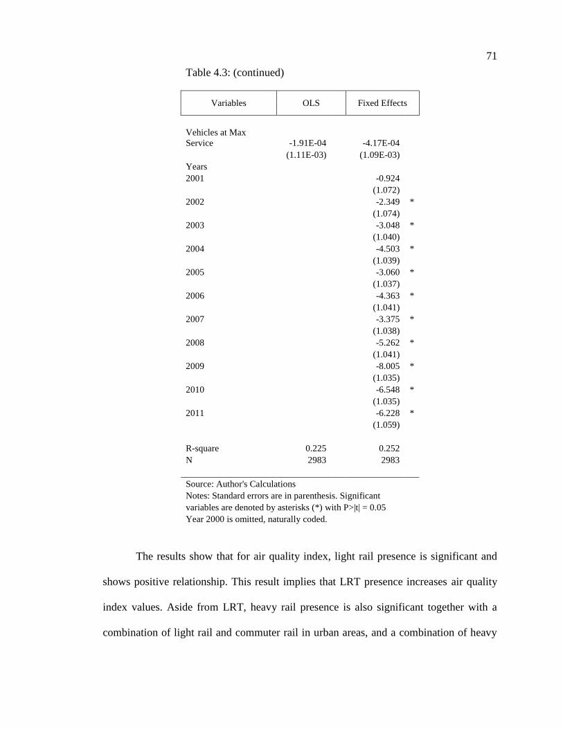
71
Table 4.3: (continued)
Variables OLS Fixed Effects
Vehicles at MaxService -1.91E-04 -4.17E-04
(1.11E-03) (1.09E-03)Years2001 -0.924
(1.072)2002 -2.349 *
(1.074)2003 -3.048 *
(1.040)2004 -4.503 *
(1.039)2005 -3.060 *
(1.037)2006 -4.363 *
(1.041)2007 -3.375 *
(1.038)2008 -5.262 *
(1.041)2009 -8.005 *
(1.035)2010 -6.548 *
(1.035)2011 -6.228 *
(1.059)
R-square 0.225 0.252N 2983 2983
Source: Author's CalculationsNotes: Standard errors are in parenthesis. Significantvariables are denoted by asterisks (*) with P>|t| = 0.05Year 2000 is omitted, naturally coded.
The results show that for air quality index, light rail presence is significant and
shows positive relationship. This result implies that LRT presence increases air quality
index values. Aside from LRT, heavy rail presence is also significant together with a
combination of light rail and commuter rail in urban areas, and a combination of heavy
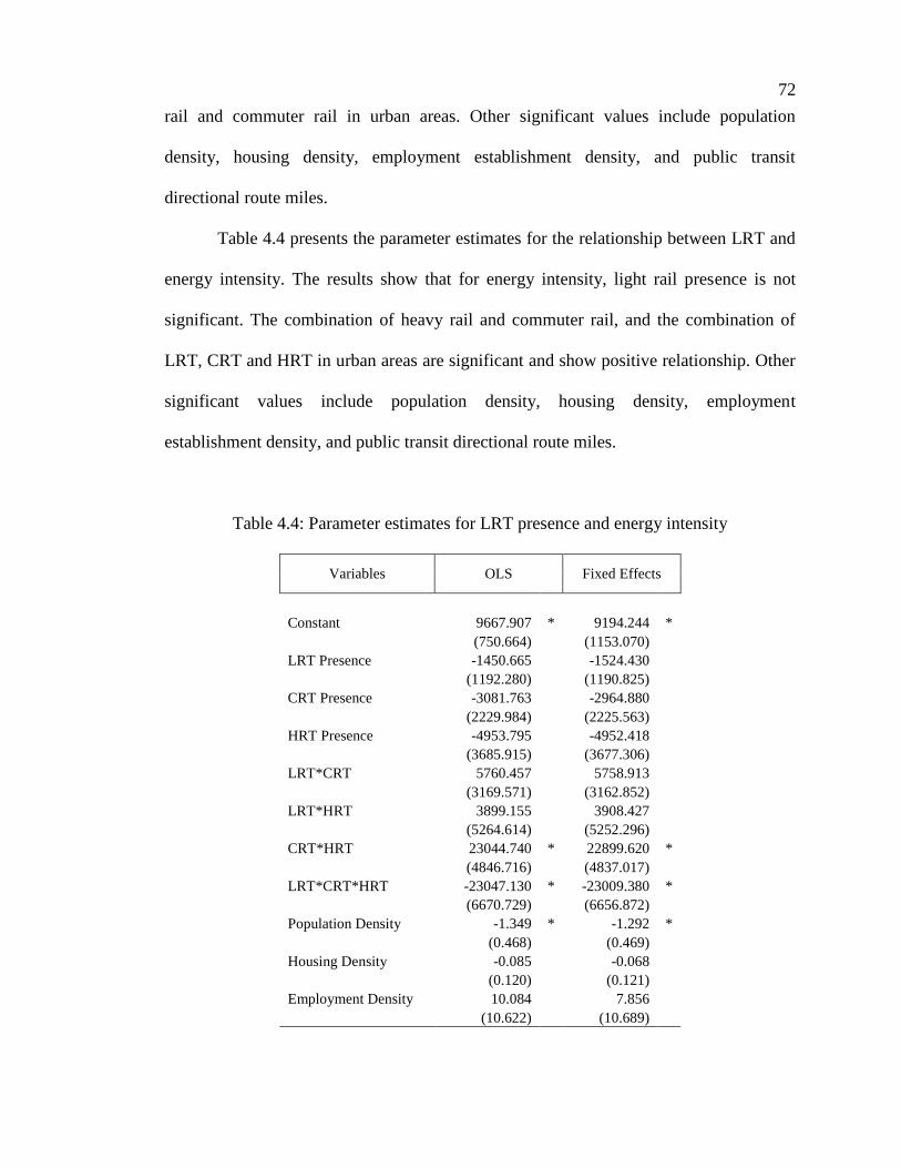
72
rail and commuter rail in urban areas. Other significant values include population
density, housing density, employment establishment density, and public transit
directional route miles.
Table 4.4 presents the parameter estimates for the relationship between LRT and
energy intensity. The results show that for energy intensity, light rail presence is not
significant. The combination of heavy rail and commuter rail, and the combination of
LRT, CRT and HRT in urban areas are significant and show positive relationship. Other
significant values include population density, housing density, employment
establishment density, and public transit directional route miles.
Table 4.4: Parameter estimates for LRT presence and energy intensity
Variables OLS Fixed Effects
Constant 9667.907 * 9194.244 *(750.664) (1153.070)
LRT Presence -1450.665 -1524.430(1192.280) (1190.825)
CRT Presence -3081.763 -2964.880(2229.984) (2225.563)
HRT Presence -4953.795 -4952.418(3685.915) (3677.306)
LRT*CRT 5760.457 5758.913(3169.571) (3162.852)
LRT*HRT 3899.155 3908.427(5264.614) (5252.296)
CRT*HRT 23044.740 * 22899.620 *(4846.716) (4837.017)
LRT*CRT*HRT -23047.130 * -23009.380 *(6670.729) (6656.872)
Population Density -1.349 * -1.292 *(0.468) (0.469)
Housing Density -0.085 -0.068(0.120) (0.121)
Employment Density 10.084 7.856(10.622) (10.689)
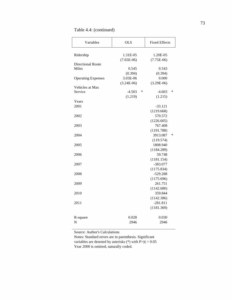
73
Table 4.4: (continued)
Variables OLS Fixed Effects
Ridership 1.31E-05 1.20E-05(7.65E-06) (7.75E-06)
Directional RouteMiles 0.545 0.543
(0.394) (0.394)Operating Expenses 3.03E-06 0.000
(3.24E-06) (3.29E-06)Vehicles at MaxService -4.503 * -4.603 *
(1.219) (1.215)Years2001 -33.121
(1219.668)2002 570.572
(1226.605)2003 767.408
(1191.788)2004 3913.087 *
(119.574)2005 1808.940
(1184.289)2006 59.748
(1181.154)2007 -383.077
(1175.834)2008 -529.288
(1175.696)2009 261.751
(1142.680)2010 359.844
(1142.386)2011 -281.811
(1181.369)
R-square 0.028 0.030N 2946 2946
Source: Author's CalculationsNotes: Standard errors are in parenthesis. Significantvariables are denoted by asterisks (*) with P>|t| = 0.05Year 2000 is omitted, naturally coded.
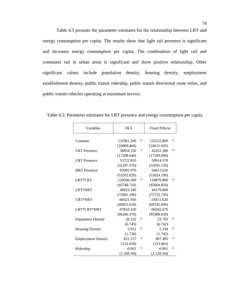
74
Table 4.5 presents the parameter estimates for the relationship between LRT and
energy consumption per capita. The results show that light rail presence is significant
and increases energy consumption per capita. The combination of light rail and
commuter rail in urban areas is significant and show positive relationship. Other
significant values include population density, housing density, employment
establishment density, public transit ridership, public transit directional route miles, and
public transit vehicles operating at maximum service.
Table 4.5: Parameter estimates for LRT presence and energy consumption per capita
Variables OLS Fixed Effects
Constant 132961.200 * 132222.800 *(10809.460) (16615.920)
LRT Presence 38854.330 * 42452.380 *(17208.040) (17169.090)
CRT Presence 53722.810 50914.570(32187.570) (32091.150)
HRT Presence 93992.970 94611.610(53202.820) (53024.190)
LRT*CRT 120506.300 * 118870.800 *(45748.710) (45604.850)
LRT*HRT 46023.540 44179.800(75991.190) (75735.720)
CRT*HRT -60421.910 -55611.620(69955.610) (69745.090)
LRT*CRT*HRT -97810.330 -96942.670(96286.370) (95988.030)
Population Density 26.332 * 23.705 *(6.745) (6.742)
Housing Density 5.951 * 5.194 *(1.738) (1.742)
Employment Density 821.157 * 907.495 *(152.658) (153.465)
Ridership -0.001 * -0.001 *(1.10E-04) (1.12E-04)
75
Table 4.5: (continued)
Variables OLS Fixed Effects
Directional RouteMiles -11.801 * -12.023 *
(5.689) (5.677)Operating Expenses 2.43E-05 0.000
(4.67E-05) (4.74E-05)Vehicles at MaxService 206.337 * 208.347 *
(17.560) (17.511)Years2001 1322.548
(17566.830)2002 17334.950
(17666.060)2003 -9395.155
(17135.210)2004 -14593.260
(17062.320)2005 -20084.240
(16998.920)2006 -20402.500
(17016.290)2007 -18210.440
(16940.270)2008 -14781.390
(16952.970)2009 24853.450
(16476.780)2010 18785.750
(16472.420)2011 32120.240
(17034.410)
R-square 0.452 0.458N 2972 2972
Source: Author's CalculationsNotes: Standard errors are in parenthesis. Significantvariables are denoted by asterisks (*) with P>|t| = 0.05Year 2000 is omitted, naturally coded.
76
Table 4.6 presents the parameter estimates for the relationship between LRT and
carbon dioxide emissions intensity. The results show that light rail presence is not
significant. The combination of heavy rail and commuter rail, and the combination of
LRT, CRT and HRT in urban areas are significant. Other significant values include
population density and public transit vehicles operating at maximum service.
Table 4.6: Parameter estimates for LRT presence and CO2 intensity
Variables OLS Fixed Effects
Constant 0.693 * 0.683 *(0.055) (0.085)
LRT Presence -0.105 -0.113(0.088) (0.087)
CRT Presence -0.211 -0.197(0.164) (0.163)
HRT Presence -0.384 -0.384(0.271) (0.270)
LRT*CRT 0.330 0.326(0.233) (0.232)
LRT*HRT 0.290 0.289(0.387) (0.386)
CRT*HRT 1.244 * 1.223 *(0.356) (0.355)
LRT*CRT*HRT -1.183 -1.170 *(0.490) (0.489)
Population Density -1.05E-04 * -9.90E-05 *(3.46E-05) (3.46E-05)
Housing Density -5.18E-06 -3.00E-06(8.86E-06) (8.88E-06)
Employment Density 7.24E-04 4.69E-04(0.001) (7.90E-04)
Ridership 7.29E-10 5.54E-10(5.62E-10) (5.69E-10)
Directional RouteMiles 1.61E-05 1.56E-05
(2.90E-05) (2.89E-05)Operating Expenses 1.25E-10 2.16E-10
(2.38E-10) (2.42E-10)
77
Table 4.6: (continued)
Variables OLS Fixed Effects
Vehicles at MaxService -2.16E-04 * -2.26E-04 *
(8.94E-05) (8.92E-05)Years2001 -0.005
(0.090)2002 0.033
(0.090)2003 0.052
(0.088)2004 -0.272 *
(0.088)2005 0.117
(0.087)2006 -0.013
(0.087)2007 -0.051
(0.087)2008 -0.076
(0.087)2009 -0.025
(0.084)2010 -0.024
(0.084)2011 -0.063
(0.087)
R-square 0.021 0.031N 2883 2883
Source: Author's CalculationsNotes: Standard errors are in parenthesis. Significantvariables are denoted by asterisks (*) with P>|t| = 0.05Year 2000 is omitted, naturally coded.
Table 4.7 presents the parameter estimates for the relationship between LRT and
carbon dioxide emissions per capita. The results show that light rail presence is not
significant. Significant values include housing density, employment establishment
78
density, public transit ridership and public transit vehicles operating at maximum
service.
Table 4.7: Parameter estimates for LRT presence and CO2 emissions per capita
Variables OLS Fixed Effects
Constant 9.695 11.258(0.788) (1.207)
LRT Presence 0.898 1.017(1.248) (1.246)
CRT Presence 3.172 3.208(2.334) (2.329)
HRT Presence -1.574 -1.592(3.858) (3.847)
LRT*CRT 4.855 4.532(3.318) (3.309)
LRT*HRT 8.484 8.298(5.511) (5.495)
CRT*HRT -6.712 -6.949(5.074) (5.061)
LRT*CRT*HRT -6.642 -5.982(6.983) (6.964)
Population Density 0.001 0.001(4.91E-04) (4.91E-04)
Housing Density 4.61E-04 * 4.54E-04 *(1.26E-04) (1.27E-04)
Employment Density 0.065 * 6.60E-02 *(0.011) (1.12E-02)
Ridership 6.41E-08 * -6.76E-08 *(8.01E-09) (8.11E-09)
Directional RouteMiles -2.98E-04 -3.22E-04
(4.13E-04) (4.12E-04)Operating Expenses -1.89E-09 -4.06E-10
(3.39E-09) (3.44E-09)Vehicles at MaxService 0.015 * 0.015 *
(0.001) (0.001)Years2001 0.001
(1.274)2002 0.862
(1.282)
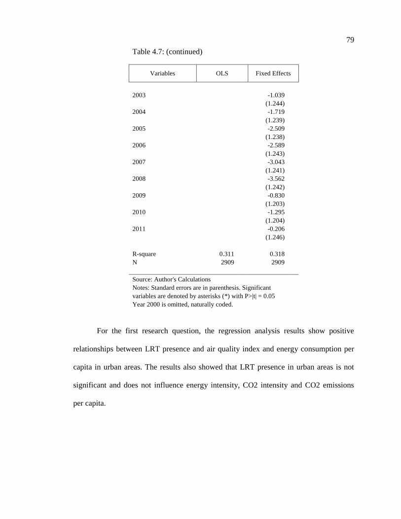
79
Table 4.7: (continued)
Variables OLS Fixed Effects
2003 -1.039(1.244)
2004 -1.719(1.239)
2005 -2.509(1.238)
2006 -2.589(1.243)
2007 -3.043(1.241)
2008 -3.562(1.242)
2009 -0.830(1.203)
2010 -1.295(1.204)
2011 -0.206(1.246)
R-square 0.311 0.318N 2909 2909
Source: Author's CalculationsNotes: Standard errors are in parenthesis. Significantvariables are denoted by asterisks (*) with P>|t| = 0.05Year 2000 is omitted, naturally coded.
For the first research question, the regression analysis results show positive
relationships between LRT presence and air quality index and energy consumption per
capita in urban areas. The results also showed that LRT presence in urban areas is not
significant and does not influence energy intensity, CO2 intensity and CO2 emissions
per capita.
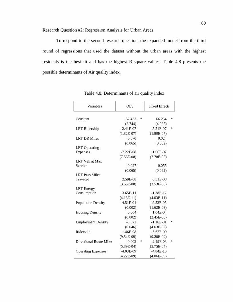
80
Research Question #2: Regression Analysis for Urban Areas
To respond to the second research question, the expanded model from the third
round of regressions that used the dataset without the urban areas with the highest
residuals is the best fit and has the highest R-square values. Table 4.8 presents the
possible determinants of Air quality index.
Table 4.8: Determinants of air quality index
Variables OLS Fixed Effects
Constant 52.433 * 66.254 *(2.744) (4.085)
LRT Ridership -2.41E-07 -5.51E-07 *(1.82E-07) (1.80E-07)
LRT DR Miles 0.070 0.024(0.065) (0.062)
LRT OperatingExpenses -7.22E-08 1.06E-07
(7.56E-08) (7.78E-08)LRT Veh at MaxService 0.027 0.055
(0.065) (0.062)LRT Pass MilesTraveled 2.59E-08 6.51E-08
(3.65E-08) (3.53E-08)LRT EnergyConsumption 3.65E-11 -1.38E-12
(4.18E-11) (4.03E-11)Population Density -4.51E-04 -9.53E-05
(0.002) (1.62E-03)Housing Density 0.004 1.04E-04
(0.002) (2.45E-03)Employment Density -0.072 -1.16E-01 *
(0.046) (4.63E-02)Ridership 1.46E-08 5.67E-09
(9.54E-09) (9.20E-09)Directional Route Miles 0.002 * 2.49E-03 *
(5.89E-04) (5.75E-04)Operating Expenses -4.03E-09 -4.84E-10
(4.22E-09) (4.06E-09)
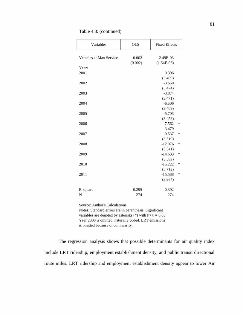
81
Table 4.8: (continued)
Variables OLS Fixed Effects
Vehicles at Max Service -0.002 -2.49E-03(0.002) (1.54E-03)
Years2001 0.396
(3.409)2002 -3.650
(3.474)2003 -3.874
(3.471)2004 -6.506
(3.409)2005 -5.703
(3.458)2006 -7.562 *
3.4792007 -9.537 *
(3.519)2008 -12.076 *
(3.541)2009 -14.633 *
(3.592)2010 -15.222 *
(3.712)2011 -15.588 *
(3.967)
R-square 0.295 0.392N 274 274
Source: Author's CalculationsNotes: Standard errors are in parenthesis. Significantvariables are denoted by asterisks (*) with P>|t| = 0.05Year 2000 is omitted, naturally coded. LRT emissionsis omitted because of collinearity.
The regression analysis shows that possible determinants for air quality index
include LRT ridership, employment establishment density, and public transit directional
route miles. LRT ridership and employment establishment density appear to lower Air
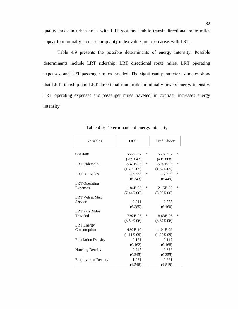
82
quality index in urban areas with LRT systems. Public transit directional route miles
appear to minimally increase air quality index values in urban areas with LRT.
Table 4.9 presents the possible determinants of energy intensity. Possible
determinants include LRT ridership, LRT directional route miles, LRT operating
expenses, and LRT passenger miles traveled. The significant parameter estimates show
that LRT ridership and LRT directional route miles minimally lowers energy intensity.
LRT operating expenses and passenger miles traveled, in contrast, increases energy
intensity.
Table 4.9: Determinants of energy intensity
Variables OLS Fixed Effects
Constant 5585.807 * 5892.607 *(269.043) (415.668)
LRT Ridership -5.47E-05 * -5.97E-05 *(1.79E-05) (1.87E-05)
LRT DR Miles -26.638 * -27.390 *(6.343) (6.449)
LRT OperatingExpenses 1.84E-05 * 2.15E-05 *
(7.44E-06) (8.09E-06)LRT Veh at MaxService -2.911 -2.755
(6.385) (6.460)LRT Pass MilesTraveled 7.92E-06 * 8.63E-06 *
(3.59E-06) (3.67E-06)LRT EnergyConsumption -4.92E-10 -1.01E-09
(4.11E-09) (4.20E-09)Population Density -0.121 -0.147
(0.162) (0.168)Housing Density -0.245 -0.329
(0.245) (0.255)Employment Density -1.081 -0.661
(4.548) (4.819)
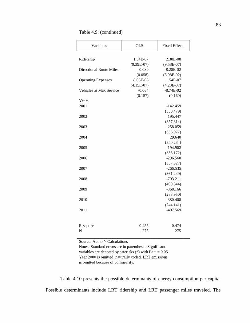
83
Table 4.9: (continued)
Variables OLS Fixed Effects
Ridership 1.34E-07 2.38E-08(9.39E-07) (9.58E-07)
Directional Route Miles -0.089 -8.28E-02(0.058) (5.98E-02)
Operating Expenses 8.03E-08 1.54E-07(4.15E-07) (4.23E-07)
Vehicles at Max Service -0.064 -8.74E-02(0.157) (0.160)
Years2001 -142.459
(350.479)2002 195.447
(357.314)2003 -258.059
(356.977)2004 29.640
(350.284)2005 -194.902
(355.172)2006 -296.560
(357.327)2007 -266.535
(361.249)2008 -703.211
(490.544)2009 -368.166
(288.950)2010 -380.408
(244.141)2011 -407.569
R-square 0.455 0.474N 275 275
Source: Author's CalculationsNotes: Standard errors are in parenthesis. Significantvariables are denoted by asterisks (*) with P>|t| = 0.05Year 2000 is omitted, naturally coded. LRT emissionsis omitted because of collinearity.
Table 4.10 presents the possible determinants of energy consumption per capita.
Possible determinants include LRT ridership and LRT passenger miles traveled. The
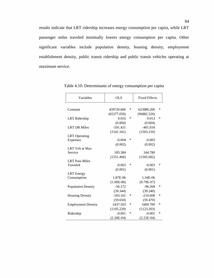
84
results indicate that LRT ridership increases energy consumption per capita, while LRT
passenger miles traveled minimally lowers energy consumption per capita. Other
significant variables include population density, housing density, employment
establishment density, public transit ridership and public transit vehicles operating at
maximum service.
Table 4.10: Determinants of energy consumption per capita
Variables OLS Fixed Effects
Constant 459720.600 * 623980.200 *(65377.050) (96882.520)
LRT Ridership 0.016 * 0.013 *(0.004) (0.004)
LRT DR Miles -591.431 -401.034(1541.341) (1503.210)
LRT OperatingExpenses -0.004 * -0.003
(0.002) (0.002)LRT Veh at MaxService 185.384 344.780
(1551.460) (1505.682)LRT Pass MilesTraveled -0.003 * -0.003 *
(0.001) (0.001)LRT EnergyConsumption 1.87E-06 1.34E-06
(1.00E-06) (9.79E-07)Population Density -56.172 -96.268 *
(39.344) (39.240)Housing Density -183.161 * -210.608 *
(59.650) (59.470)Employment Density 2437.503 * 3469.700 *
(1105.229) (1123.203)Ridership -0.001 * -0.001 *
(2.28E-04) (2.23E-04)
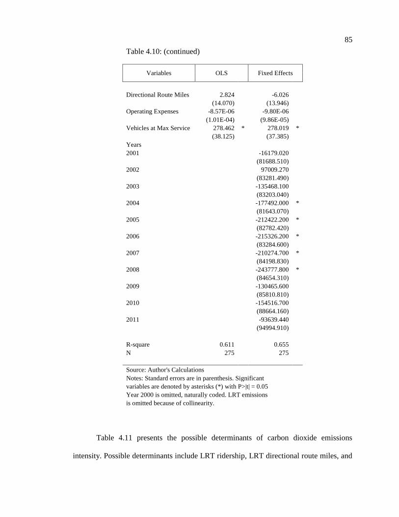
85
Table 4.10: (continued)
Variables OLS Fixed Effects
Directional Route Miles 2.824 -6.026(14.070) (13.946)
Operating Expenses -8.57E-06 -9.80E-06(1.01E-04) (9.86E-05)
Vehicles at Max Service 278.462 * 278.019 *(38.125) (37.385)
Years2001 -16179.020
(81688.510)2002 97009.270
(83281.490)2003 -135468.100
(83203.040)2004 -177492.000 *
(81643.070)2005 -212422.200 *
(82782.420)2006 -215326.200 *
(83284.600)2007 -210274.700 *
(84198.830)2008 -243777.800 *
(84654.310)2009 -130465.600
(85810.810)2010 -154516.700
(88664.160)2011 -93639.440
(94994.910)
R-square 0.611 0.655N 275 275
Source: Author's CalculationsNotes: Standard errors are in parenthesis. Significantvariables are denoted by asterisks (*) with P>|t| = 0.05Year 2000 is omitted, naturally coded. LRT emissionsis omitted because of collinearity.
Table 4.11 presents the possible determinants of carbon dioxide emissions
intensity. Possible determinants include LRT ridership, LRT directional route miles, and
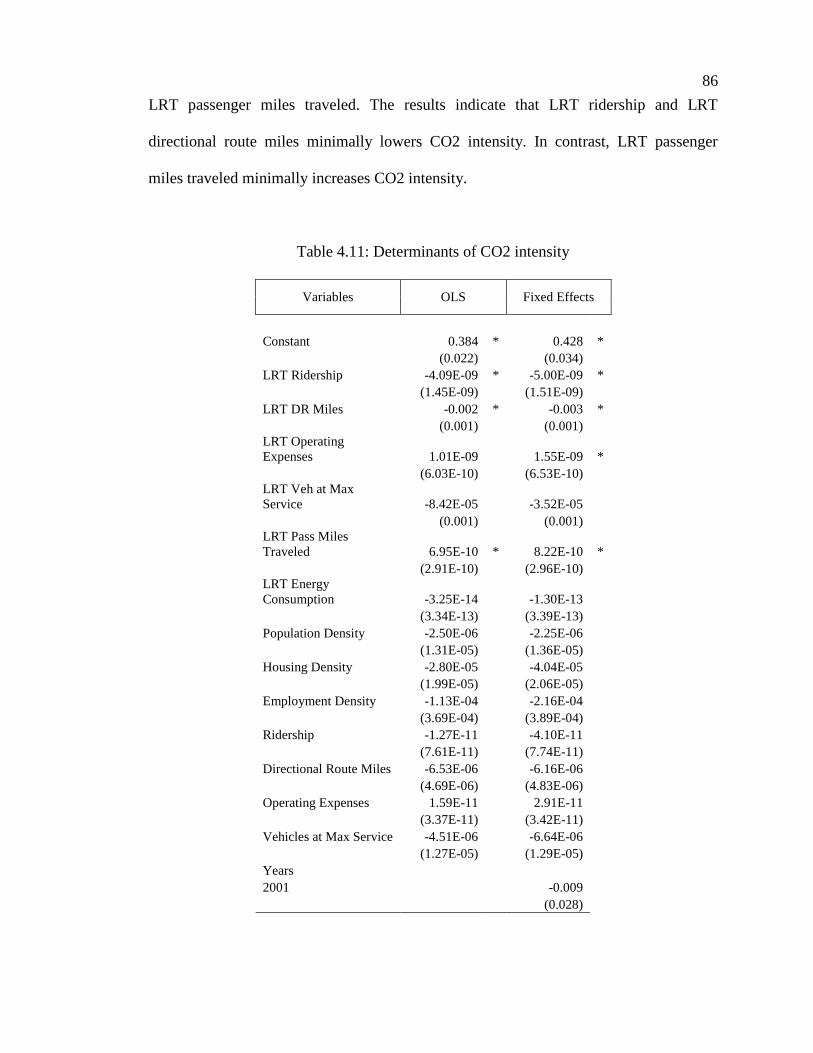
86
LRT passenger miles traveled. The results indicate that LRT ridership and LRT
directional route miles minimally lowers CO2 intensity. In contrast, LRT passenger
miles traveled minimally increases CO2 intensity.
Table 4.11: Determinants of CO2 intensity
Variables OLS Fixed Effects
Constant 0.384 * 0.428 *(0.022) (0.034)
LRT Ridership -4.09E-09 * -5.00E-09 *(1.45E-09) (1.51E-09)
LRT DR Miles -0.002 * -0.003 *(0.001) (0.001)
LRT OperatingExpenses 1.01E-09 1.55E-09 *
(6.03E-10) (6.53E-10)LRT Veh at MaxService -8.42E-05 -3.52E-05
(0.001) (0.001)LRT Pass MilesTraveled 6.95E-10 * 8.22E-10 *
(2.91E-10) (2.96E-10)LRT EnergyConsumption -3.25E-14 -1.30E-13
(3.34E-13) (3.39E-13)Population Density -2.50E-06 -2.25E-06
(1.31E-05) (1.36E-05)Housing Density -2.80E-05 -4.04E-05
(1.99E-05) (2.06E-05)Employment Density -1.13E-04 -2.16E-04
(3.69E-04) (3.89E-04)Ridership -1.27E-11 -4.10E-11
(7.61E-11) (7.74E-11)Directional Route Miles -6.53E-06 -6.16E-06
(4.69E-06) (4.83E-06)Operating Expenses 1.59E-11 2.91E-11
(3.37E-11) (3.42E-11)Vehicles at Max Service -4.51E-06 -6.64E-06
(1.27E-05) (1.29E-05)Years2001 -0.009
(0.028)
87
Table 4.11: (continued)
Variables OLS Fixed Effects
2002 0.013(0.029)
2003 -0.019(0.029)
2004 0.002(0.028)
2005 -0.018(0.029)
2006 -0.029(0.029)
2007 -0.028(0.029)
2008 -0.062 *(0.029)
2009 -0.036(0.030)
2010 -0.045(0.031)
2011 -0.047
R-square 0.454 0.477N 275 275
Source: Author's CalculationsNotes: Standard errors are in parenthesis. Significantvariables are denoted by asterisks (*) with P>|t| = 0.05Year 2000 is omitted, naturally coded. LRT emissionsis omitted because of collinearity.
Table 4.12 presents the possible determinants of carbon dioxide emissions per
capita. Possible determinants include housing density, employment establishment
density, public transit ridership and public transit vehicles operating at maximum
service. None of the LRT characteristics in the study dataset affect CO2 emissions per
capita.
88
Table 4.12: Determinants of CO2 emissions per capita
Variables OLS Fixed Effects
Constant 33.270 * 48.137 *(5.061) (7.534)
LRT Ridership 9.05E-07 * 6.37E-07(3.36E-07) (3.39E-07)
LRT DR Miles -0.112 -0.114(0.119) (0.117)
LRT OperatingExpenses -3.40E-07 * -1.70E-07
(1.40E-07) (1.47E-07)LRT Veh at MaxService -0.013 0.002
(0.120) (0.117)LRT Pass MilesTraveled -1.61E-07 * -1.30E-07
(6.75E-08) (6.64E-08)LRT EnergyConsumption 1.32E-10 8.61E-11
(7.74E-11) (7.62E-11)Population Density -0.003 -0.005
(0.003) (0.003)Housing Density -0.013 * -0.016 *
(0.005) (0.005)Employment Density 0.129 0.182 *
(0.086) (0.087)Ridership -8.60E-08 * -9.11E-08 *
(1.77E-08) (1.74E-08)Directional Route Miles 6.29E-04 8.35E-04
(0.001) (0.001)Operating Expenses 3.08E-09 4.25E-09
(7.81E-09) (7.67E-09)Vehicles at Max Service 0.018 * 1.77E-02 *
(0.003) (0.003)Years2001 -1.172
(6.353)2002 6.916
(6.477)2003 -9.547
(6.471)2004 -11.941
(6.349)2005 -15.970 *
(6.438)
89
Table 4.12: (continued)
Variables OLS Fixed Effects
2006 -16.253 *(6.477)
2007 -16.225 *(6.548)
2008 -19.695 *(6.583)
2009 -13.194 *(6.673)
2010 -14.116 *(6.895)
2011 -11.442(7.388)
R-square 0.429 0.487N 275 275
Source: Author's CalculationsNotes: Standard errors are in parenthesis. Significantvariables are denoted by asterisks (*) with P>|t| = 0.05Year 2000 is omitted, naturally coded. LRT emissionsis omitted because of collinearity.
The second question deals with finding possible determinants of the selected
environmental sustainability indicators. The series of regression analysis indicate that
factors that influence environmental sustainability varies and depends on the outcome
variables: air quality index, energy intensity, energy consumption per capita, CO2
intensity and CO2 emissions per capita. The most common variables in all the regression
analyses combined that provide the most influence with the selected environmental
sustainability indicators are light rail ridership, light rail passenger miles traveled, light
rail operating expenses, and light rail directional route miles.
90
Impact Analysis Results
The models with the highest variances explained by the independent variables are
the expanded models from the regression analysis without the urban areas with highest
residuals. Using these models for addressing the research questions, the actual values
and the predicted values of the selected environmental sustainability indicators are
compared with respect to the following changes in variables: 1) change in the number of
urban areas with light rail presence based on size of the urban areas; and 2) change in
level of light rail ridership. The classification for the size of the urban areas is based on
the urban area classification used by the National Transit Database, as follows:
a) small size urban areas – urban areas with population less than 200,000;
b) medium size urban areas – urban areas with population greater than
200,000; and
c) large size urban areas – urban areas with population greater than 1
million.
For changes in light rail transit ridership, a 25 percent, 50 percent, 75 percent and
100 percent increase from the actual light rail ridership is assumed. The average actual
and the average predicted values for each selected environmental sustainability
indicators are compared with the average predicted values for changes in light rail
presence in urban areas and light rail ridership.
Table 4.13 presents the impact analysis summary for changes in light rail
presence in urban areas.
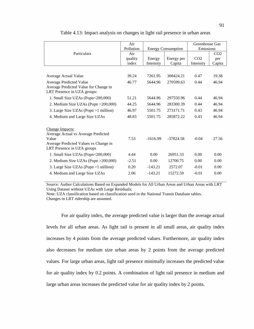
91
Table 4.13: Impact analysis on changes in light rail presence in urban areas
Particulars
AirPollution Energy Consumption
Greenhouse GasEmissions
Airqualityindex
EnergyIntensity
Energy perCapita
CO2Intensity
CO2per
Capita
Average Actual Value 39.24 7261.95 308424.21 0.47 19.38
Average Predicted Value 46.77 5644.96 270599.63 0.44 46.94Average Predicted Value for Change inLRT Presence in UZA groups:
1. Small Size UZAs (Popn<200,000) 51.21 5644.96 297550.96 0.44 46.94
2. Medium Size UZAs (Popn >200,000) 44.25 5644.96 283300.39 0.44 46.94
3. Large Size UZAs (Popn >1 million) 46.97 5501.75 273171.71 0.43 46.94
4. Medium and Large Size UZAs 48.83 5501.75 285872.22 0.43 46.94
Change Impacts:Average Actual vs Average PredictedValue 7.53 -1616.99 -37824.58 -0.04 27.56Average Predicted Values vs Change inLRT Presence in UZA groups
1. Small Size UZAs (Popn<200,000) 4.44 0.00 26951.33 0.00 0.00
2. Medium Size UZAs (Popn >200,000) -2.51 0.00 12700.75 0.00 0.00
3. Large Size UZAs (Popn >1 million) 0.20 -143.21 2572.07 -0.01 0.00
4. Medium and Large Size UZAs 2.06 -143.21 15272.59 -0.01 0.00
Source: Author Calculations Based on Expanded Models for All Urban Areas and Urban Areas with LRTUsing Dataset without UZAs with Large Residuals;Note: UZA classification based on classification used in the National Transit Database tables.Changes in LRT ridership are assumed.
For air quality index, the average predicted value is larger than the average actual
levels for all urban areas. As light rail is present in all small areas, air quality index
increases by 4 points from the average predicted values. Furthermore, air quality index
also decreases for medium size urban areas by 2 points from the average predicted
values. For large urban areas, light rail presence minimally increases the predicted value
for air quality index by 0.2 points. A combination of light rail presence in medium and
large urban areas increases the predicted value for air quality index by 2 points.
92
For energy intensity, the average predicted value is lower than the average actual
levels for energy intensity in all urban areas. When light rail is present in all small urban
areas, the results indicate that there are no changes in the predicted values for energy
intensity. The same result is projected when light rail is present in medium size urban
areas. For large size urban areas and for the combination of medium size and large size
urban areas that have light rail presence, the average actual predicted values decreased.
For energy consumption per capita, the average predicted value is also lower than
the average actual values for energy consumption per capita. When light rail is present is
small urban areas, there is no change from the predicted values. For medium size and
large size urban areas, average predicted values increased by 907 points. Similarly, when
light rail is present in all medium and large size urban areas, average predicted values for
energy consumption per capita also increased.
For CO2 intensity, the average predicted value is lower by 0.4 points than the
average actual values for CO2 intensity in all urban areas. When light rail is present in
small and medium areas, there are no changes in the predicted values. However, as light
rail is present in large size urban areas and in both medium and large size areas, CO2
intensity decreases by 0.1 points.
For CO2 emissions per capita, the average predicted value is lower than the
actual values for CO2 emissions per capita by 3.75 points. However, regardless of
whether light rail is present in any of the urban area groupings, there are no changes in
the average actual predicted values for CO2 emissions per capita.
The results of the impact analysis indicates that for air quality index, more light
rail in large urban areas have lower positive effect. For energy intensity, the results
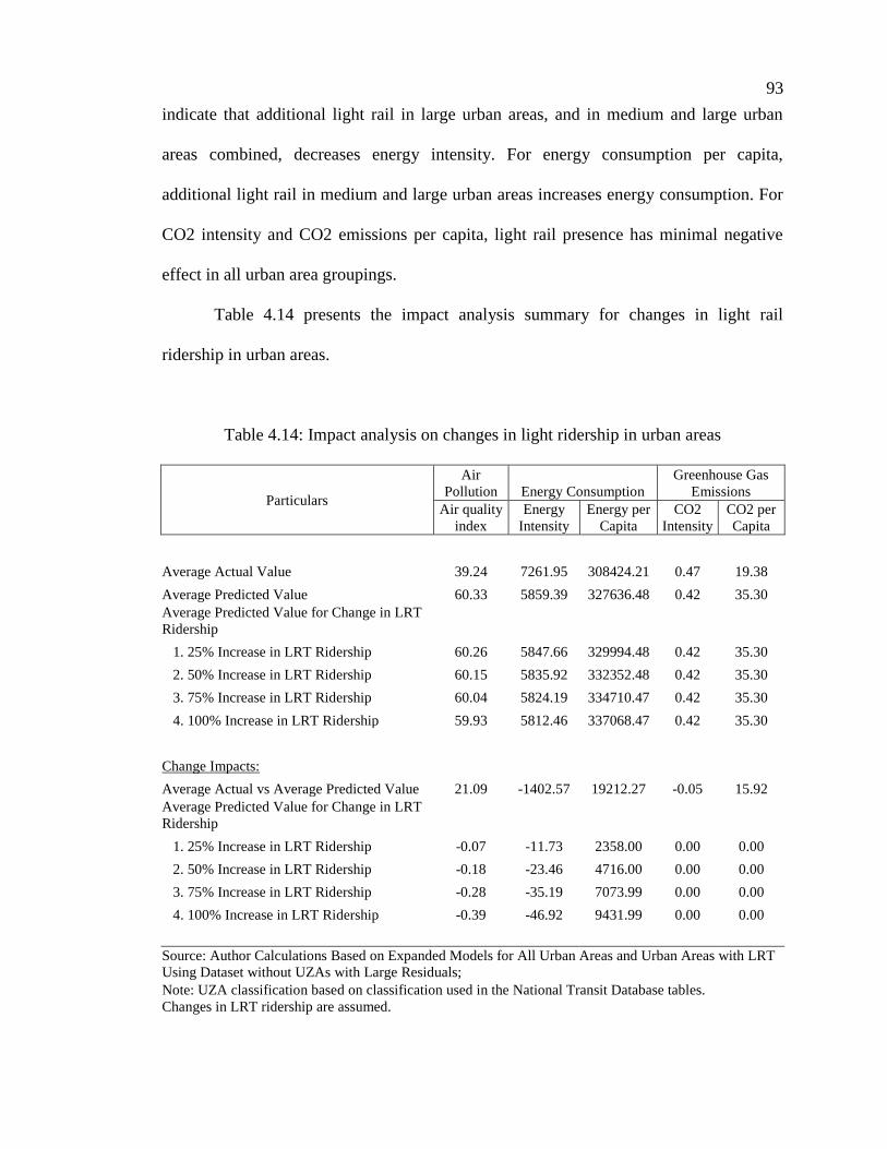
93
indicate that additional light rail in large urban areas, and in medium and large urban
areas combined, decreases energy intensity. For energy consumption per capita,
additional light rail in medium and large urban areas increases energy consumption. For
CO2 intensity and CO2 emissions per capita, light rail presence has minimal negative
effect in all urban area groupings.
Table 4.14 presents the impact analysis summary for changes in light rail
ridership in urban areas.
Table 4.14: Impact analysis on changes in light ridership in urban areas
Particulars
AirPollution Energy Consumption
Greenhouse GasEmissions
Air qualityindex
EnergyIntensity
Energy perCapita
CO2Intensity
CO2 perCapita
Average Actual Value 39.24 7261.95 308424.21 0.47 19.38
Average Predicted Value 60.33 5859.39 327636.48 0.42 35.30Average Predicted Value for Change in LRTRidership
1. 25% Increase in LRT Ridership 60.26 5847.66 329994.48 0.42 35.30
2. 50% Increase in LRT Ridership 60.15 5835.92 332352.48 0.42 35.30
3. 75% Increase in LRT Ridership 60.04 5824.19 334710.47 0.42 35.30
4. 100% Increase in LRT Ridership 59.93 5812.46 337068.47 0.42 35.30
Change Impacts:
Average Actual vs Average Predicted Value 21.09 -1402.57 19212.27 -0.05 15.92Average Predicted Value for Change in LRTRidership
1. 25% Increase in LRT Ridership -0.07 -11.73 2358.00 0.00 0.00
2. 50% Increase in LRT Ridership -0.18 -23.46 4716.00 0.00 0.00
3. 75% Increase in LRT Ridership -0.28 -35.19 7073.99 0.00 0.00
4. 100% Increase in LRT Ridership -0.39 -46.92 9431.99 0.00 0.00
Source: Author Calculations Based on Expanded Models for All Urban Areas and Urban Areas with LRTUsing Dataset without UZAs with Large Residuals;Note: UZA classification based on classification used in the National Transit Database tables.Changes in LRT ridership are assumed.
94
For air quality index, the average predicted value is larger than the actual values
for air quality index in urban areas. A 25 percent increase in LRT ridership lowers the
predicted air quality index values in urban areas by less than 1 point. As LRT ridership
increases to 50 percent, 75 percent and 100 percent than the actual LRT ridership in the
dataset, reduction in the levels for predicted air quality index increases, although very
minimal and less than 1 point.
For energy intensity, average predicted value is lower than the average actual
value for all urban areas. A 25 percent increase in LRT ridership lowers the average
predicted value for energy intensity by 11 points. As LRT ridership increases to 50
percent, 75 percent and 100 percent, average predicted values decreases by larger
margins, from 23 points, 35 points and 46 points, respectively.
For energy consumption per capita, average predicted value is larger than the
average actual value for energy consumption per capita. A 25 percent increase in LRT
ridership increases the average predicted value by 2358 points. As LRT ridership
increases to 50 percent, 75 percent and 100 percent, average predicted values decreases
by larger margins, from 4716 points, 7073 points and 9431 points, respectively.
For CO2 intensity, average actual predicted value is lower by 0.05 points than the
actual value. The results indicate that there are no changes in predicted values regardless
of changes in LRT ridership.
For CO2 emissions per capita, average actual predicted value is higher than the
average actual value by 15.92 points. The results also indicate that there are no changes
in predicted values regardless of changes in LRT ridership.
95
The results of the impact analysis on changes in LRT ridership indicates that an
increase in LRT riders lowers air quality index and lowers energy intensity. For energy
consumption per capita, increase in LRT ridership increases the predicted values. More
LRT riders will increase the level of energy consumption in the urban area.
Chapter Summary
The results of the bivariate regressions and the series of multiple regression
analysis for this study indicate the light rail presence affects the selected environmental
sustainability indicators at varying degrees. In terms of identifying the possible
determinants of the selected environmental sustainability indicators, urban area
characteristics, light rail characteristics and public transit characteristics affect selected
environmental sustainability indicators at varying degrees. The results of the impact
analysis, however, indicate that light rail presence has significant effects on minimizing
air pollution and energy consumption. The effect of light rail presence on minimizing
greenhouse gas emissions is not significant. In terms of light rail ridership, the impact
analysis results imply that more light rail riders lowers air quality index levels (although
minimally) and that more light rail riders lowers energy intensity. The results also imply
that increases in LRT ridership do not significantly affect minimizing energy
consumption per capita and minimizing greenhouse gas emissions.
The next chapter will provide a discussion of the results and the implications of
these results to environmental policy, energy policy, and transportation policy. The next
chapter will also discuss how the results validated the initial hypotheses previously
outlined in the study.
96
CHAPTER 5: DISCUSSION OF RESULTS
This chapter provides a discussion of the results of the analysis and its
implications to environmental policy, energy policy, transportation policy, and
sustainable transportation. To begin this discussion, a summary of the results of the
analysis is presented in the context of testing and validating the hypotheses that were
previously outlined. The discussions seek to enrich the analysis of the results and
connect the findings to policy implications.
The research questions for this study are expressed as follows:
1. How does light rail presence affect environmental sustainability indicators in
urban areas?
2. For urban areas that have light rail systems, how do light rail, public transit,
and urban area characteristics affect environmental sustainability indicators?
General findings of the study indicate that light rail presence affect the selected
environmental sustainability indicators in urban areas at varying degrees. Based on the
analyses of variances, the best models for analysis among the series of regressions
conducted are the third round regression results that yielded the highest R-square values.
Using the third round regression results – with the dataset without the urban areas that
have the highest residuals, light rail presence is a significant variable for all five
environmental sustainability indicators under the basic model. As additional variables
are included in the analysis to control for effects of urban area and public transit
97
characteristics, light rail presence is only significant for air quality index, but various
combinations with other forms of passenger rail help maintain its significance for energy
intensity, energy consumption per capita and CO2 intensity. Light rail presence is not
significant for CO2 emissions per capita.
In determining possible determinants of environmental sustainability among
urban areas with light rail, the third round of regression results indicate the best model
fits to understand influential factors. Significant variables also vary per environmental
sustainability indicator. The most common indicators for all five models are housing
density, light rail ridership, light rail directional route miles, light rail operating
expenses, total public transit ridership and total number of vehicles operating at
maximum service. LRT ridership and total public transit directional route miles affect
the air quality index, while LRT ridership, LRT directional route miles and LRT
operating expenses affect energy intensity. Housing density, employment density, total
public transit ridership and total number of vehicles operating at maximum service affect
energy consumption per capita. LRT directional route miles, LRT operating expenses,
LRT passenger miles traveled and housing density affect CO2 intensity. Finally, housing
density, total public transit ridership and the total number of vehicles operating at
maximum service affect CO2 emissions per capita.
The directions and strength of the relationship among these variables with the
selected environmental sustainability indicators will be discussed in the context of
testing and validating the hypotheses that were previously outlined in the study. Using
the third round regression results, the significant variables for each model are
highlighted.
98
Validating the Hypotheses
The results of the analysis are discussed to test and validate each of the following
hypotheses:
1. Light rail presence in urban areas has a significant influence on minimizing
air pollution, energy use and greenhouse gas emissions.
Light rail presence in urban areas has a significant influence on minimizing air
pollution, and provides significant influence over minimizing energy use and minimizing
greenhouse gas emissions through a combination of other forms of passenger rail in
urban areas.
Light rail presence increases the air quality index values. Heavy rail presence
also increases the air quality index values. The combination of light rail and commuter
rail presence and heavy rail and commuter rail presence both lower air quality index
values. Higher population density and housing density increases air quality index
values, while higher employment establishment density lowers the air quality index
values. An increase in total public transit directional route miles also increases air
quality index.
Light rail presence does not provide significant effects for energy consumption
indicators, but combined with other forms of passenger rail, light rail presence provides
some significant effects. The combination of light rail, heavy rail and commuter rail in
urban areas lowers energy intensity. In contrast, the combination of heavy rail and
commuter rail increases energy intensity. An increase in population density and the
number of vehicles operating at maximum service for public transit lowers energy
intensity. For energy per capita, a combination of light rail and commuter rail presence
99
increases energy consumption per capita. Higher population density, housing density and
employment establishment density in urban areas also increases energy consumption per
capita. An increase in the number of vehicles operated at maximum service also
increases energy per capita. However, an increase in total public transit ridership and
total directional route miles for public transit lowers energy per capita. This may be due
to the spreading out of energy consumption to all members of the population.
For minimizing greenhouse gas emissions, light rail presence is not a significant
factor in understanding CO2 intensity and CO2 emissions per capita. However, the
combination of light rail, heavy rail and commuter rail presence in urban areas lowers
CO2 intensity. In contrast, however, the combination of heavy rail presence and
commuter rail presence increases CO2 intensity. This may be due to the larger traffic
volumes carried by both heavy rail and commuter rail modes. The number of vehicles
operating at maximum service also lowers CO2 intensity, although with minimal effect.
Population density, housing density and employment establishment density also provide
minimal positive effects on CO2 emissions per capita. Public transit ridership, on the
other hand, provides minimal negative effect for CO2 emissions per capita.
In sum, light rail presence has a more significant influence over air quality index
than all the other selected environmental sustainability indicators for energy
consumption and greenhouse gas emissions. However, a combination of light rail
presence with other modes in urban areas makes light rail significant for affecting energy
consumption and greenhouse gas emissions.
2. Light rail characteristics affect environmental sustainability goals.
100
A number of light rail characteristics affect environmental sustainability goals.
An increase in light rail ridership both lowers air quality index values and energy
intensity. An increase in light rail directional route miles lowers energy intensity, but
increases CO2 intensity. An increase in light rail operating expenses both minimally
increases energy intensity and CO2 intensity. Finally, an increase in light rail passenger
miles traveled also minimally increases CO2 intensity.
3. Public transit characteristics affect environmental sustainability goals.
Three public transit characteristics affect environmental sustainability goals. An
increase in public transit ridership lowers energy per capita and CO2 per capita. An
increase in directional route miles increases air quality index, while vehicles operated at
maximum service increases energy per capita and CO2 per capita.
4. Urban densities affect environmental sustainability goals.
Among the three urban densities described in this study (population, housing and
employment establishment density), only housing and employment establishment
density show significant effects. Housing density affects energy consumption per capita,
CO2 intensity and CO2 emissions per capita. An increase in housing density lowers
energy per capita, CO2 intensity and CO2 emissions per capita. Employment
establishment density, in contrast, increases energy consumption per capita. The more
employment establishments in the urban area, the more energy is consumed.
Policy Implications
The primary contribution of this study is to provide empirical evidence on the
influence of light rail presence on environmental sustainability in urban areas. Results
showed that indeed, light rail presence influences the selected environmental
101
sustainability indicators at varying degrees. Light rail presence, as it appears in the
results of the analysis, has more influence on air quality index values than all the other
selected environmental sustainability indicators.
Based on the results, it appears that light rail presence increases the air quality
index. Contrary to the notion that light rail is environmentally sustainable and that light
rail minimizes air pollution, it appears that light rail does not help improve air quality in
the area. However, taking into consideration that air quality is only one aspect of
environmental sustainability, this study cannot make any conclusions on the
environmental sustainability of light rail transit based one aspect alone. The results also
indicate that an increase in light rail presence can also lower energy intensity. In this
case, the result indicates that light rail presence lowers the amount of energy consumed
to achieve travel output (passenger miles traveled). The goal of the study to determine
the influence of light rail on selected environmental sustainability is achieved through
empirical evidence, but the result may not be necessarily conclusive as expected.
While the results focuses on light rail presence as main determinant for selected
environmental sustainability indicators, the influence of heavy rail and the combination
of light rail and other forms of transit in urban areas should also be considered as
significant. Similar to the results with light rail presence, heavy rail presence also
contributes to increases in air quality index values in the area.
Aside from enhancing the current literature on the environmental sustainability
of light rail systems, the results of the analysis identified factors that influence
environmental sustainability. By identifying influential factors, policy can be directed
towards improving these factors so that the benefit of environmental sustainability is
102
achieved. Noting that light rail ridership influences the selected environmental
sustainability indicators, policy may be directed towards increasing light rail ridership in
urban areas. The results of analysis can be used to aid policy formulation and analysis
through more discussions on the significant factors that influence environmental
sustainability.
The policy implications of the results of the analysis in this study are more
relevant to the policy discussions on environmental policy, energy policy and
transportation policy. Since this study is also done in the context of sustainability, the
results also provide some insights on how the environmental sustainability goals of
sustainable transportation area achieved.
For environmental policy, the findings of this study add to the discussion on the
benefits and effects of light rail presence to air pollution and the use of energy resources.
The government’s environmental policy, typically established by the EPA, has focused
traditionally on conservation of natural resources, but in the 1960’s, policy focus on
environment covered concerns over public health, which includes controlling air and
water pollution, and limiting exposure to toxic chemicals (Kraft & Furlong, 2010). The
findings of this study show that light rail increases air pollution, along with other forms
of rail transit, in urban areas. However, since air pollution is only one aspect related to
environmental sustainability, this study cannot conclude that light rail presence causes
air pollution. There are many more factors that can be considered to boost this analysis,
as well as methods that can specifically address providing causality for environmental
sustainability goals.
103
Another aspect within environmental policy is climate change. The goal of
climate change policy is to reduce the rate and mitigate the risks of climate change for
future generations. This relates to lessening the use of fossil fuels, which leads to less
CO2 emissions. Does LRT presence reduce CO2 emissions in urban areas? The results
of the analysis using the existing data indicate the LRT presence is not significant for
minimizing greenhouse gas emissions. With regards to air quality, the results of the
analysis indicate that LRT increases the air quality index values, but the relationship
cannot be causal, since there are many other omitted variables in the study that may
provide a better insight on the relationship between LRT and air quality.
Another finding of this study is the effect of light rail presence on energy
intensity and energy consumption per capita. While energy intensity and energy
consumption per capita is measured at the urban area level, light rail presence effects are
miniscule compared to all possible effects of other factors that contribute to energy
consumption. These other factors may come from other sectors of society, and not only
from the transportation sector. The same could also be said for CO2 intensity and CO2
emissions. The impact of light rail presence may be too miniscule or virtually absent on
the selected environmental sustainability indicators because of there a many other
unknown contributing factors that are also not included in the study. Hence, to relate the
findings to overall environmental policy, focus must be on the value of the empirical
findings on improving the discussion on the impact of light rail presence on the selected
environmental sustainability goals, rather than focusing on concluding that light rail
presence causes air pollution, energy consumption or greenhouse gas emissions. To
104
provide causality, a different modeling approach is needed, and may be a subject for
future study on this topic.
Environmental policy is also connected with energy policy, as energy sources
contribute to harmful emissions to the environment that affect the population.
Environmental policy also covers energy policy, especially with the enactment of the
Energy Policy Act of 2005 (PL 109-58) and subsequent related energy policies such as
the Energy Independence and Security Act of 2009 (PL 110-140) and with the funding
of energy policy in the American Recovery and Reinvestment Act of 2009 (PL 111-5)
(Kraft & Furlong, 2010). The findings of this study also reinforce the discussion for
energy resource use, especially on how light rail presence affects energy consumption.
Light rail presence is supposed to lower energy intensity, but the variable in the model is
not significant. A different modeling approach in a future study may provide a more
definitive conclusion on the impact of light rail presence on energy consumption.
Aside from the notion that energy policy is a natural resource policy component
of environmental policy, the other policy component of energy policy covers
environmental protection. Given that light rail operates on electricity as fuel, less CO2 is
emitted in the atmosphere. The policy decisions involving the use of alternative fuel
vehicles and alternative fuel for public transit depends on government’s motivations and
commitment to protect the environment and lessen the effects of greenhouse gas
emissions. The findings of this study indirectly reinforces the argument that rail in
general has environmental protection benefits, if this analysis is interpreted based on the
benefits of the use of electricity as fuel in transportation instead of petroleum based fuels
that have more CO2 emissions. However, careful consideration must be included when
105
making generalizations regarding the possible benefits of the use of electricity as source
of energy. Electricity is also coal-powered, which is also a form of fossil fuel. In
addition, the waste generated for producing and renewing electricity may not be evident
in areas that have LRT, but it is a possibility that the waste will be released in another
part of the urban area, which may also be in an area away from the most populous, most
congested and most dense parts of the urban area.
The findings also relate to implications on transportation policy. Transportation
policy covers modal selection for public transit, and investments on public transit over
other transportation investments on infrastructure such as highways, roads and bridges.
Are there investments being made in providing sustainable public transit options? The
findings of this study indicate that more operating expenses on light rail transit
minimally increases energy intensity and CO2 intensity, but does not necessary cause
energy intensity and CO2 intensity. A comparison of energy intensity and CO2 intensity
as well as how energy consumption and CO2 emissions relate to ridership may provide
additional insights than the findings from the regression analysis.
Table 5.1 presents a comparative analysis of light rail, heavy rail, commuter rail,
and bus systems on energy intensity, CO2 intensity, energy consumption per public
transit ridership and CO2 emissions per public transit ridership. Using 2011 data from
the dataset used in the study and figures from the National Transit Database, the results
show that of all four public transit systems compared, light rail does not have the lowest
energy intensity, lowest CO2 intensity, lowest CO2 emissions per ridership and lowest
CO2 emissions per ridership. Based on the comparative analysis, heavy rail has the least
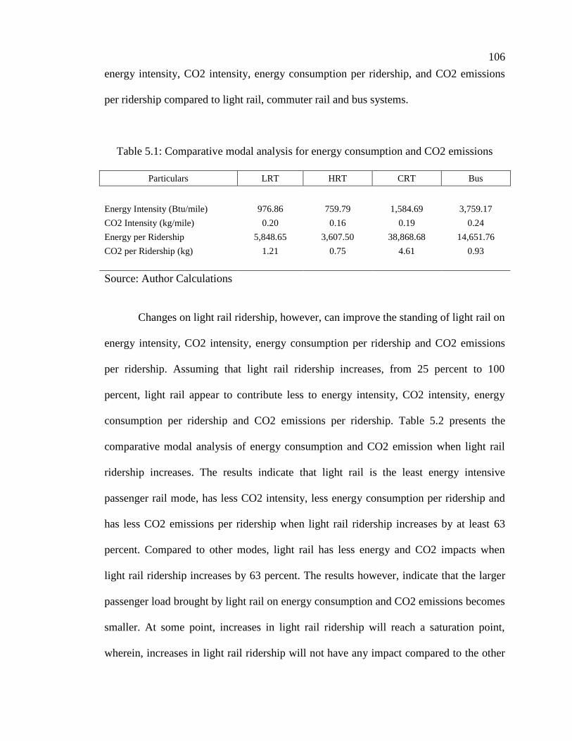
106
energy intensity, CO2 intensity, energy consumption per ridership, and CO2 emissions
per ridership compared to light rail, commuter rail and bus systems.
Table 5.1: Comparative modal analysis for energy consumption and CO2 emissions
Particulars LRT HRT CRT Bus
Energy Intensity (Btu/mile) 976.86 759.79 1,584.69 3,759.17
CO2 Intensity (kg/mile) 0.20 0.16 0.19 0.24
Energy per Ridership 5,848.65 3,607.50 38,868.68 14,651.76
CO2 per Ridership (kg) 1.21 0.75 4.61 0.93
Source: Author Calculations
Changes on light rail ridership, however, can improve the standing of light rail on
energy intensity, CO2 intensity, energy consumption per ridership and CO2 emissions
per ridership. Assuming that light rail ridership increases, from 25 percent to 100
percent, light rail appear to contribute less to energy intensity, CO2 intensity, energy
consumption per ridership and CO2 emissions per ridership. Table 5.2 presents the
comparative modal analysis of energy consumption and CO2 emission when light rail
ridership increases. The results indicate that light rail is the least energy intensive
passenger rail mode, has less CO2 intensity, less energy consumption per ridership and
has less CO2 emissions per ridership when light rail ridership increases by at least 63
percent. Compared to other modes, light rail has less energy and CO2 impacts when
light rail ridership increases by 63 percent. The results however, indicate that the larger
passenger load brought by light rail on energy consumption and CO2 emissions becomes
smaller. At some point, increases in light rail ridership will reach a saturation point,
wherein, increases in light rail ridership will not have any impact compared to the other
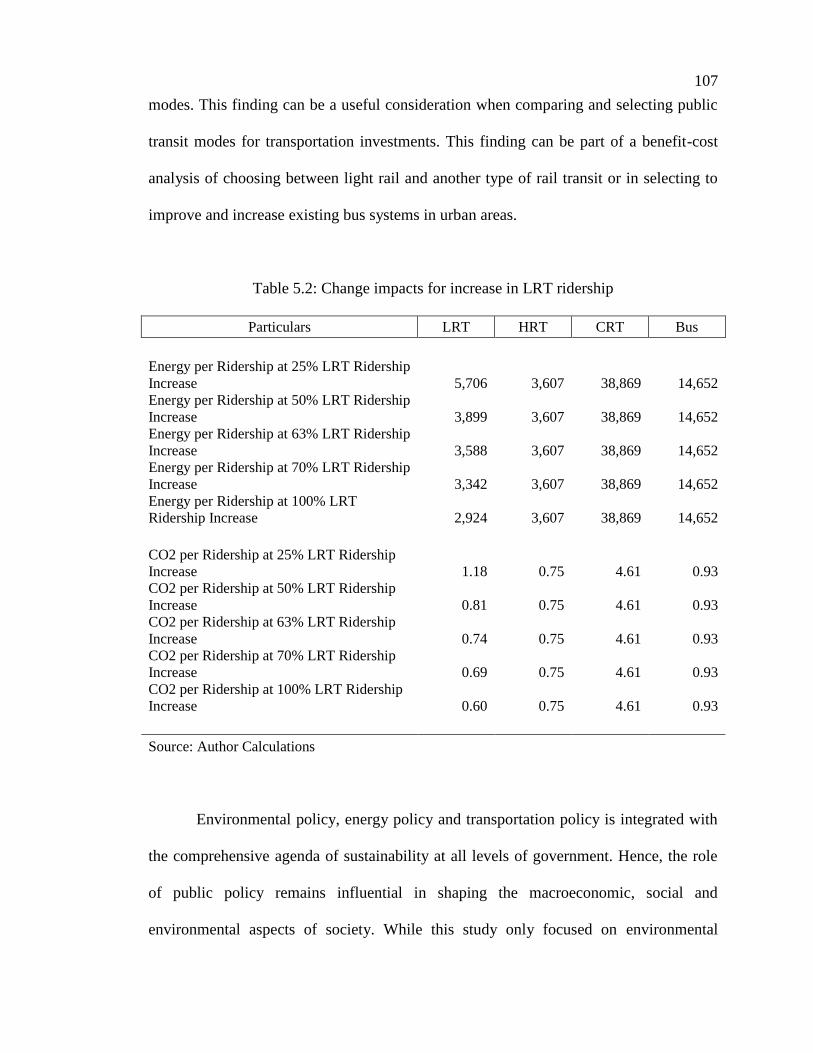
107
modes. This finding can be a useful consideration when comparing and selecting public
transit modes for transportation investments. This finding can be part of a benefit-cost
analysis of choosing between light rail and another type of rail transit or in selecting to
improve and increase existing bus systems in urban areas.
Table 5.2: Change impacts for increase in LRT ridership
Particulars LRT HRT CRT Bus
Energy per Ridership at 25% LRT RidershipIncrease 5,706 3,607 38,869 14,652Energy per Ridership at 50% LRT RidershipIncrease 3,899 3,607 38,869 14,652Energy per Ridership at 63% LRT RidershipIncrease 3,588 3,607 38,869 14,652Energy per Ridership at 70% LRT RidershipIncrease 3,342 3,607 38,869 14,652Energy per Ridership at 100% LRTRidership Increase 2,924 3,607 38,869 14,652
CO2 per Ridership at 25% LRT RidershipIncrease 1.18 0.75 4.61 0.93CO2 per Ridership at 50% LRT RidershipIncrease 0.81 0.75 4.61 0.93CO2 per Ridership at 63% LRT RidershipIncrease 0.74 0.75 4.61 0.93CO2 per Ridership at 70% LRT RidershipIncrease 0.69 0.75 4.61 0.93CO2 per Ridership at 100% LRT RidershipIncrease 0.60 0.75 4.61 0.93
Source: Author Calculations
Environmental policy, energy policy and transportation policy is integrated with
the comprehensive agenda of sustainability at all levels of government. Hence, the role
of public policy remains influential in shaping the macroeconomic, social and
environmental aspects of society. While this study only focused on environmental
108
sustainability, the study demonstrated how light rail presence affects environmental
sustainability even through a selected number of indicators for environmental
sustainability goals. Further research on this subject is encouraged, in addition to
additional study on understanding light rail and its impacts on social and economic
sustainability. The subject of improving this research and suggestions for policy
recommendations are discussed in the concluding chapter for this study.
109
CHAPTER 6: SUMMARY, CONCLUSIONS AND RECOMMENDATIONS
This chapter presents the summary, conclusions and recommendations of this
study on environmental sustainability of light rail systems in urban areas. Suggestions
for further improving this research are also outlined in this chapter.
Summary
The objective of this dissertation is to understand how light rail presence affects
environmental sustainability in urban areas. For urban areas with existing light rail
systems, this study also seeks to determine how light rail, urban area and public transit
characteristics affect environmental sustainability. Environmental sustainability
indicators were selected based on the environmental sustainability goals of minimizing
air pollution, energy resource use and greenhouse gas emissions. Environmental
sustainability goals were measured as air quality index, energy intensity, energy
consumption per capita, carbon dioxide emissions intensity, and carbon dioxide
emissions per capita as outcome variables. Using urban area and public transit data from
2000 to 2011, the impacts of light rail presence and other forms of passenger rail transit
on selected environmental sustainability indicators were estimated through bivariate
regression analysis and a series of multiple regressions with light rail, urban area and
public transit characteristics. Findings indicate that light rail presence affects
environmental sustainability in varying degrees for each of the outcome variables. Light
rail presence increases the predicted values for air quality index, but does not
significantly affect energy intensity, energy per capita, CO2 intensity and CO2 per
110
capita. Possible determinants of the selected environmental sustainability indicators
include light rail ridership, light rail directional route miles, light rail operating expenses,
and light rail passenger miles traveled. Housing density and employment density also
significantly affects environmental sustainability indicators. Public transit ridership,
directional route miles, and the number of vehicles operating at maximum service also
affect environmental sustainability. Further research on light rail presence is encouraged
to improve the results of the analysis of environmental sustainability in urban areas.
Conclusions
Light rail presence affects environmental sustainability at varying degrees,
depending on the approach of the analysis and the environmental sustainability measures
used. The bivariate regression results established individual independent variable effects
for each of the selected environmental sustainability indicators in the study. The results
of the regression analyses, however, demonstrate a more refined representation of the
effects of light rail presence and other significant variables on environmental
sustainability indicators. While regression analysis results provide significant effects
between the explanatory variables and the outcome variables, the results are not
interpreted as causal effects. Light rail presence increases air quality index values but
this study does not conclude that light rail causes air pollution to increase. While light
rail presence does not have significant relationships with energy intensity, energy
consumption per capita, CO2 emissions intensity and CO2 emissions per capita, this
study also does not conclude that light rail presence can neither increase nor decrease the
selected environmental sustainability indicators. This study establishes the relationships
111
and the direction of these relationships between light rail presence and environmental
sustainability in urban areas in the United States.
Given the results of the analysis, the main point of the study on the
environmental sustainability of light rail transit is to establish the fact that light rail
presence is not sufficient to encourage sustainability in urban areas. Making the light rail
transit available in urban areas is not the primary driving factor that makes it
sustainability. One of the findings of this study indicates that LRT ridership can be the
driving factor that can make LRT systems sustainable. People should be able to utilize
LRT when available to provide an impact. If LRT is available and less people ride the
LRT systems, and more people prefer to ride privately owned vehicles instead of public
transit, then LRT does not appear to be sustainable. LRT ridership is the key to influence
environmental sustainability in urban areas.
Policy Recommendations
A key policy recommendation arising from the realization that LRT ridership
may provide the key to influence environmental sustainability is to focus on increasing
LRT ridership in urban areas where LRT is available. Policy recommendations resulting
from the conclusions of this study are focused on directing existing environmental,
energy and transportation policies to increase light rail transit ridership. As presented in
Table 5.2, the results of the comparative modal analysis indicate that light rail transit
becomes the least energy intensive and least CO2 emissions intensive compared to other
rail transit modes and bus system when light rail ridership is increased by at least 63
percent from the existing 2011 ridership levels. Based on available 2011 data from the
National Transit Database, ridership levels for light rail is at 434 million in 2011. Light
112
rail ridership should increase to about 708 million to be able to be less energy intensive
and less CO2 emissions intensive than heavy rail, commuter rail and bus systems. Policy
recommendations and strategies for increasing ridership include, but not limited to the
following needs:
a) additional public relations campaign on the benefits of riding light rail transit
for urban areas that have existing LRT systems in place;
b) additional light rail presence in urban areas as an alternative public transit
option, although this requires a thorough feasibility study as well as capital
outlay and investments from government and private sector partnerships;
c) incentives to ride light rail instead of privately owned vehicles through fare
pricing, fuel tax incentives, subsidies;
d) provisions for park and ride facilities within the proximity of light rail transit
station.
These policy recommendations require budget appropriations, legislation and other
policy discussions for implementing and operating light rail transit systems. The
decision to build light rail transit systems on urban areas depends on the demand for rail
transit and other considerations such as population growth, economic feasibility and
public transit ridership. In addition, the cultural aspect and attitudes toward riding light
rail and other forms of public transit should be considered. In the United States, majority
of the population still prefer to ride their privately owned vehicles instead of public
transit for ease of mobility and convenience. Providing access to public transit options
may not be sufficient when public attitudes and demand for public transit is low. In
essence, establishing a light rail transit system is dependent on whether people will
113
actually ride light rail transit when available. This applies also to other more energy
efficient forms of public transportation. Hence, in considering choices for building and
operating public transit systems as well as high volume highways, all aspects of
environmental, economic and social sustainability must be covered in the analysis to be
able to provide a comprehensive view on whether public transit systems adhere to the
principles of the sustainable transportation agenda.
Limitations of the Study
While this study provided empirical evidence on the relationship between LRT
and environmental sustainability indicators and possible determinants, the study has
many limitations. While the study is guided by the triple bottom line aspects of
sustainability, the primary focus of this analysis is focused on environmental
sustainability. However, discussions indirectly cover the social and economic aspects of
sustainable transportation, especially when trying to provide an explanation why LRT
presence is significant for air quality and energy consumption per capita, but not
significant for energy intensity and CO2 emissions variables. In addition, the study did
not cover the institutional and political aspects of sustainability. From a conceptual
framework, the role of institutions and politics can provide additional insights and
explanations to the relationships between LRT and sustainability.
As a form of empirical evidence, the findings of this study reinforces the notion
that light rail has environmental sustainability impacts. However, the findings of this
study are also limited to urban areas, and are limited to available data and measurement
variables in the existing statistical system. The definitions and the measurement of the
variables used in the study may change over time to capture the changes in the units of
114
analysis and other factors, which may alter and be different from the initial findings of
the study.
While the impact of light rail on environmental sustainability in urban areas is
examined, this study also takes into account the areas that have other forms of rail transit
in the urban areas, such as heavy rail and commuter rail. The presence of other forms of
public transit may also affect environmental sustainability in the area, and the results of
the analysis can broaden the understanding on the benefits of rail transit in general on
environmental sustainability.
Bus systems are not included in the empirical analysis of study. Bus systems
have been initially considered for this study together with other passenger rail transit
modes. However, all the urban areas covered in the study have bus systems in place,
thereby providing no variation for comparison. Bus systems, on the other hand, are
included in some policy discussions in the study, but the transit modes considered in this
study are passenger rail modes.
The policy discussions and the results of the study do not directly address the
following issues: a) policy debates on which transit option is a better alternative for
urban areas; b) comparison between light rail systems and bus systems; c) comparison
between rail investments and highway investments; and d) light rail impacts on urban
development patterns. Focus on light rail and environmental sustainability provides
additional value on the literature for sustainable transportation and sustainable public
transit options.
The discussions for this study are focused on light rail presence and
environmental sustainability goals. The resulting analysis does not make conclusions on
115
the overall sustainability of light rail systems since the study is only focused on one of
the three aspects of sustainable transportation. The three aspects of sustainable
transportation, also referred to as the “triple bottom line” are social, economic and
environmental sustainability.
Finally, data used as environmental sustainability indicators are limited to data
and information that are available in the existing statistical system. Data for variables
that represent possible determinants of environmental sustainability are also limited to
available data and information at the geographic area level of analysis. The available
data and information provided a constraint in covering the analysis of all the
environmental sustainability goals that are provided in sustainable transportation
definition (Hall, 2006). Since secondary data is used, there are may be missing values in
the dataset and the author has no control over the validity of data that was entered in the
databases at the time of research. In addition to missing values, test for the measurement
validity of the variables used in the study are limited. While collinearity issues have been
addressed in the regression analysis, a possible endogeneity problem with the variables
was not explicitly addressed in the analysis and discussion. Additional tests and
variables that were previously omitted should be included in future analysis related to
the environmental sustainability of LRT systems
With respect to the overall research goals for this study, the results of the analysis
provide the relationships among dependents and independent variables through empirical
data. Other considerations to be included in selecting additional variables to improve this
research may include the purposes and motivations why LRT is built and operated in
urban areas, the regional effects, city effects, and the attitudes of the public on LRT
116
ridership, environmental sustainability and identifying factors that motivate and enable
people to ride the LRT and other public transit.
Suggestions for Further Research
Given the findings of the study, suggestions for further research include
addressing the limitations of the study and improving the analysis of LRT and
sustainability. Additional environmental sustainability indicators can be identified and
included in this study, provided that data is available at the urban area level. Suggestions
include indicators for other environmental sustainability goals that were not covered in
this study such as minimizing health and environmental damage, maintaining high
environmental quality and human health standards, minimizing the production of noise,
minimizing the use of land, and recycling. These additional environmental sustainability
goals are based on the definition of sustainable transportation compiled by Hall (2006).
A comparative modal analysis on energy consumption and CO2 emissions
indicated that based on data from 2011, light rail is not the least energy intensive, and
least CO2 emissions intensive among other modes of rail transit and bus systems. A
similar method of analysis used in this study focusing on heavy rail presence, commuter
rail presence and bus system presence can be conducted using specific modal
characteristics similar to the variables used for light rail. While the models for the first
research question addressed heavy rail and commuter rail presence, the analysis can be
enhanced with the inclusion of heavy rail and commuter rail characteristics as
independent variables, and compared with light rail impacts.
Other statistical and regression analysis approaches can also be utilized in future
analysis that captures all aspects of environmental sustainability and sustainable
117
transportation. The use of the fixed effects models in the regression analysis enhanced
the analysis by removing possible confounding and spurious variables brought about my
certain conditions and events that may also influence environmental sustainability. Other
statistical and econometric modeling approaches include the use of structural models,
general equilibrium models and other techniques for analysis.
A similar approach for analysis used in this study can be utilized in considering
other aspects of sustainability, such as economic, social and institutional sustainability.
By identifying measurable goals for each of these aspects, and finding relevant and
measurable indicators for the same geographical urban area level, the same analysis
using the same dataset can also be conducted. By covering all aspects of sustainability, a
more comprehensive picture can be provided on the state of LRT systems as a
sustainable public transit option.
Final Note
As a final note, the results of this analysis established a small portion of
improving the understanding of the environmental sustainability of light rail systems.
This dissertation only focused on one aspect of sustainable transportation (environmental
sustainability) and on one mode of public transit (light rail transit). Suggestions for
further research include expanding the focus of the study on other aspects of
sustainability such as economic and social sustainability. Aside from expanding this
study to other aspects of sustainability, analysis can also be expanded to other modes of
transportation, specifically for public transit. Further research is also encouraged for
identifying additional sustainability indicators and for discussing other possible
determinants for sustainability.
118
REFERENCES
Arndt, J. C., Morgan, C., Overman, J. H., Clower, T. L., Weinstein, B. L., & Seman, M.(2009). Transportation, Social and Economic Impacts of Light and Commuter Rail.Texas Transportation Institute. Texas: National Technical Information Service.
Bhatta, S., & Drennan, M. (2003). The economic benefits of public investment intransportation: A review of recent literature. Journal of Planning Education andResearch , 22, 88-296.
Black, J. A., Paez, A., & Suthanaya, P. A. (2002). Sustainable Urban Transportation:Performance Indicators and Some Analytical Approaches. Journal of Urban Planningand Development , 128 (4), 184-209.
Black, W. R. (1996). Sustainable transportation: a US Perspective. Journal of TransportGeography , 4 (3), 151-159.
Black, W. R., & Sato, N. (2007). From Global Warning to Sustainable Transport 1989-2006. International Journal of Sustainable Transportation , 1 (2), 73-89.
Carpenter, T. (1994). The environmental impact of railways. West Sussex, England:John Wiley and Sons, Ltd.
Cervero, R. (1984). Light Rail Transit and Urban Development. Journal of AmericanPlanning Association , 50 (2), 133-147.
Daly, H. (1990). Toward some operational principles of sustainable development.Ecological Economics , 2, 1-6.
De Bruijn, H., & Veeneman, W. (2009). Decision-making for light rail. TransportationResearch Part A , 43 (4), 349-359.
Department of Commerce. (2011, August 24). Federal Register Vol. 76, No. 164.Retrieved from Census Bureau: http://www.census.gov/geo/www/ua/fedregv76n164.pdfEnvironmental Protection Agency. (1996). Indicators of the Environmental Impacts ofTransportation: Highway, Rail, Aviation and Maritime Transport.
Etsy, D. C., Levy, M., Srebotnjak, T., & De Sherbinin, A. (2005). 2005 EnvironmentalSustainability Index: Benchmarking National Environmental Stewardship. New Haven:Yale Center for Environmental Law and Policy.
European Conference of Ministers of Transport (ECMT). (1994). Light Rail TransitSystems. Paris, France: Organisation for Economic Co-Operation and Development(OECD).
119
Federal Transit Administration (FTA). (2012a, November 6). National TransitDatabase. Retrieved January 10, 2013, from Transit Agency Information:http://www.ntdprogram.gov/ntdprogram/
Federal Transit Administration (FTA). (2013). National Transit Database Glossary.Retrieved January 14, 2013, from National Transit Database Glossary:http://www.ntdprogram.gov/ntdprogram/Glossary.htm
Fielding, G. J. (1995). Transit in American Cities. In S. Hanson, The Geography ofUrban Transportation. New York: The Guilford Press.
Fietelson, E. (1994). The potential of rail as an environmental solution: setting theagenda. Transportation Research Part A , 28 (3), 209-221.
Giuliano, G. (2004). Land Use Impacts of Transportation Investments: Highway andTransit. In S. Hanson, & G. G., The Geography of Urban Transportation, 3rd Edition.
Gomez-Ibanez, J. A. (1985). A Dark Side to Light Rail?: The Experience of Three NewTransit Systems. Journal of American Planning Association , 51 (3), 337-351.
Greenberg, J. B. (2005). Light Rail Transit in the United States since 1980: If you Buildit, will they come? PhD Dissertation, University of Louisville, School of Urban andPublic Affairs, Louisville, Kentucky.
Greene, D. L., & Wegener, M. (1997). Sustainable transport. Journal of TransportGeography , 5 (3).
Greg, M., Kimble, M., Nellthorp, J., & Kelly, C. (2010). Sustainability Assessment: TheDefinition Deficit. International Journal of Sustainable Transportation , 4 (4), 189-211.
Hall, R. P. (2006). Understanding and Applying the Concept of SustainableDevelopment to Transportation Planning and Decision-Making in the U.S. PhDDissertation, Massachusetts Institute of Technology.
Hass-Klau, C., Crampton, G., & Benjari, R. (2004). Economic impact of light rail: Theresults of 15 urban areas in France, Germany, UK and North America. Environmentaland Transport Planning .
Hensher, D. A. (2007). Sustainable public transport systems: Moving towards a value formoney and network-based approach and away from blind commitment. TransportationPolicy , 14 (1), 98-102.
Horner, M. W., & Grubesic, T. H. (2001). A GIS-Based planning approach to locatingurban rail terminals. Transportation , 28, 55-77.
120
Jeon, C. M. (2007). Incorporating Sustainability into Transportation Planning andDecision Making: Definitions, Performance Measures and Evaluation. PhDDissertation, Georgia Institute of Technology.
Jeon, C. M., & Amekudzi, A. (2005). Addressing Sustainability in TransportationSystems: Definitions, Indicators, and Metrics. Journal of Infrastructure Systems , 11, 31-50.
Joumard, R. (2011). Environmental Sustainability Assessments: Toward a NewFramework. International Journal of Sustainable Society , 3 (2), 133-150.
Joumard, R., Gudmundsson, H., & Folkeson, L. (2011). Framework for AssessingIndicators of Environmental Impacts in the Transport Sector. Conference Paper inTransportation Research Board 90th Annual Meeting, Washington, D.C.
Kenworthy, J. (2008). An International Review of The Significance of Rail inDeveloping More Sustainable Urban Transport Systems in Higher Income Cities. WorldTransport Policy and Practice , 14 (2), 21-37.
Komiyama, H., & Kazuhiko, T. (2006). Sustainability Science: building a newdiscipline. Sustainability Science , 1 (1), 1-6.
Kraft, M. E., & Furlong, S. R. (2010). Public Policy: Politics, Analysis and Alternatives,3rd Edition. Washington, DC: CQ Press.
Lavery, T., & Kanaroglou, P. (2012). Rediscovering light rail: assessing the potentialimpacts of a light rail transit line on transit oriented development and transit ridership.Transportation Letters: the International Journal of Transportation Research , 16 (4),211-226.
Litman, T. (2007). Developing Indicators for Comprehensive and Sustainable TransportPlanning. Transportation Research Record , 2017, 10-15.
Litman, T. (2012b). Evaluating Rail Transit Criticism. British Columbia, Canada:Victoria Transport Policy Institute. Retrieved January 13, 2013, fromhttp://vtpi.org/railcrit.pdf
Litman, T. (2012a). Rail Transit in America: A Comprehensive Evaluation of Benefits.British Columbia, Canada: Victoria Transport Policy Insitute. Retrieved fromhttp://www.vtpi.org/railben.pdf
Litman, T. (2004). Rail Transit in America: Comprehensive evaluation of benefits.Retrieved from http://www.vtpi.org/railben.pdf
121
Meyer, M. D. (2008). Public Transportation and Environment. In M. Kutz,Environmentally Conscious Transportation (pp. 15-46). Hoboken, New Jersey: JohnWiley and Sons, Inc.
Newman, P., & Kenworthy, J. R. (1999). Sustainability and Cities: OvercomingAutomobile Independence. Washington, D.C.: Island Press.
Organisation for Economic Co-Operation and Development (OECD). (1997). TowardsSustainable Transportation: The Vancouver Conference. OECD Proceedings: TowardsSustainable Transportation. Vancouver, British Columbia: Organisation for EconomicCo-Operation and Development.
Pope, J., Annandale, D., & Morrison-Saunders, A. (2004). Conceptualising sustainabilityassessment. Environmental Impact Assessment Review , 24 (6), 595-616.
Rees, W. E. (1995). Achieving Sustainability: Reform or Transformation? Journal ofPlanning Literature , 9 (4), 343-361.
Richardson, B. C. (2005). Sustainable transport: analysis frameworks. Journal ofTransport Geography , 13, 29-39.
Richardson, B. C. (1999). Toward a Policy on a Sustainability Transportation System.Transportation Research Record , 1670, 27-34.
Rodrigue, J.-P., Comtois, C., & Slack, B. (2006). The Geography of Transport Systems.New York: Routledge.
Schiller, P. L., Bruun, E. C., & Kenworthy, J. R. (2010). An Introduction to SustainableTransportation: Policy Planning and Implementation. Washington, D.C.: Earthscan.
Semmens, J. (2006). Are Benefits of Light Rail Worth Sacrifices of Foregone BusService? Journal of Transportation Law, Logistics and Policy , 73 (4), 453-462.
Shane, M. A., & Graedel, T. E. (2000). Urban Sustainability Metrics: A Provisional Set.Journal of Environmental Planning and Management , 43 (5), 643-663.
The Centre for Sustainable Transportation (CST). (2005, March 31). DefiningSustainable Transportation. Winnepeg, Manitoba, Canada. Retrieved fromhttp://cst.uwinnipeg.ca/documents/Defining_Sustainable_2005.pdf
The Centre for Sustainable Transportation (CST). (2002, October). Definition andVision of Sustainable Transportation. Mississauga, Ontario, Canada.
Thompson, G. L. (2003). Defining an Alternative Future: Birth of the LIght RailMovement in North America. Transportation Research Board.
122
Topalovic, P., Carter, J., Topalovic, M., & Krantzberg, G. (2012). Light Rail Transit inHamilton: Health, Environmental and Economic Impact Analysis. Social IndicatorsResearch , 108 (2), 329-350.
Van Diepen, A., & Voogd, H. (2001). Sustainability and Planning: Does Urban FormMatter? International Journal of Sustainable Development , 4 (1), 59-74.
Vuchic, V. R. (1999). Transportation for Livable Cities. New Brunswick, New Jersey:Center for Urban Policy Research.
World Commission on Environment and Development (WCED). (1987). Our CommonFuture. United Kingdom: Oxford University Press.
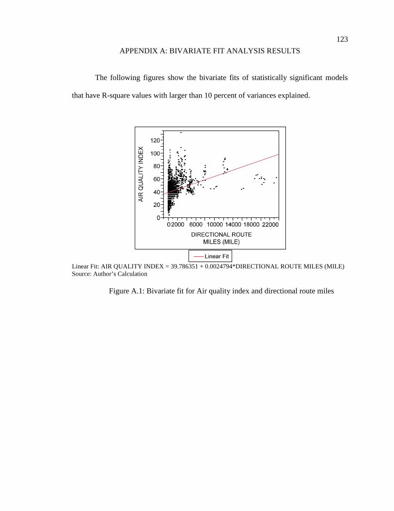
123
APPENDIX A: BIVARIATE FIT ANALYSIS RESULTS
The following figures show the bivariate fits of statistically significant models
that have R-square values with larger than 10 percent of variances explained.
Linear Fit: AIR QUALITY INDEX = 39.786351 + 0.0024794*DIRECTIONAL ROUTE MILES (MILE)Source: Author’s Calculation
Figure A.1: Bivariate fit for Air quality index and directional route miles
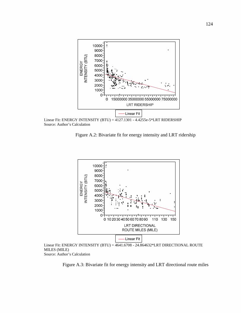
124
Linear Fit: ENERGY INTENSITY (BTU) = 4127.1301 - 4.4255e-5*LRT RIDERSHIPSource: Author’s Calculation
Figure A.2: Bivariate fit for energy intensity and LRT ridership
Linear Fit: ENERGY INTENSITY (BTU) = 4641.6708 - 24.864632*LRT DIRECTIONAL ROUTEMILES (MILE)Source: Author’s Calculation
Figure A.3: Bivariate fit for energy intensity and LRT directional route miles
ENER
GY
INTE
NSI
TY(B
TU)
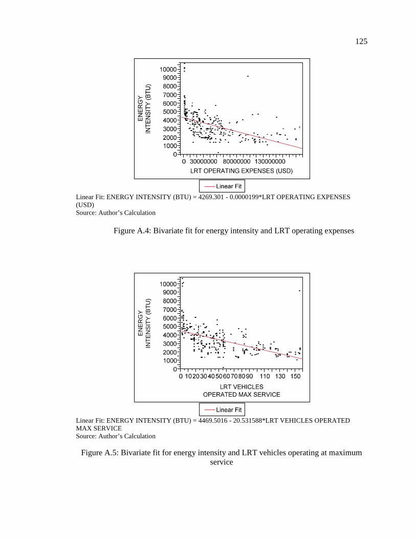
125
Linear Fit: ENERGY INTENSITY (BTU) = 4269.301 - 0.0000199*LRT OPERATING EXPENSES(USD)Source: Author’s Calculation
Figure A.4: Bivariate fit for energy intensity and LRT operating expenses
Linear Fit: ENERGY INTENSITY (BTU) = 4469.5016 - 20.531588*LRT VEHICLES OPERATEDMAX SERVICESource: Author’s Calculation
Figure A.5: Bivariate fit for energy intensity and LRT vehicles operating at maximumservice
ENER
GY
INTE
NSI
TY(B
TU)
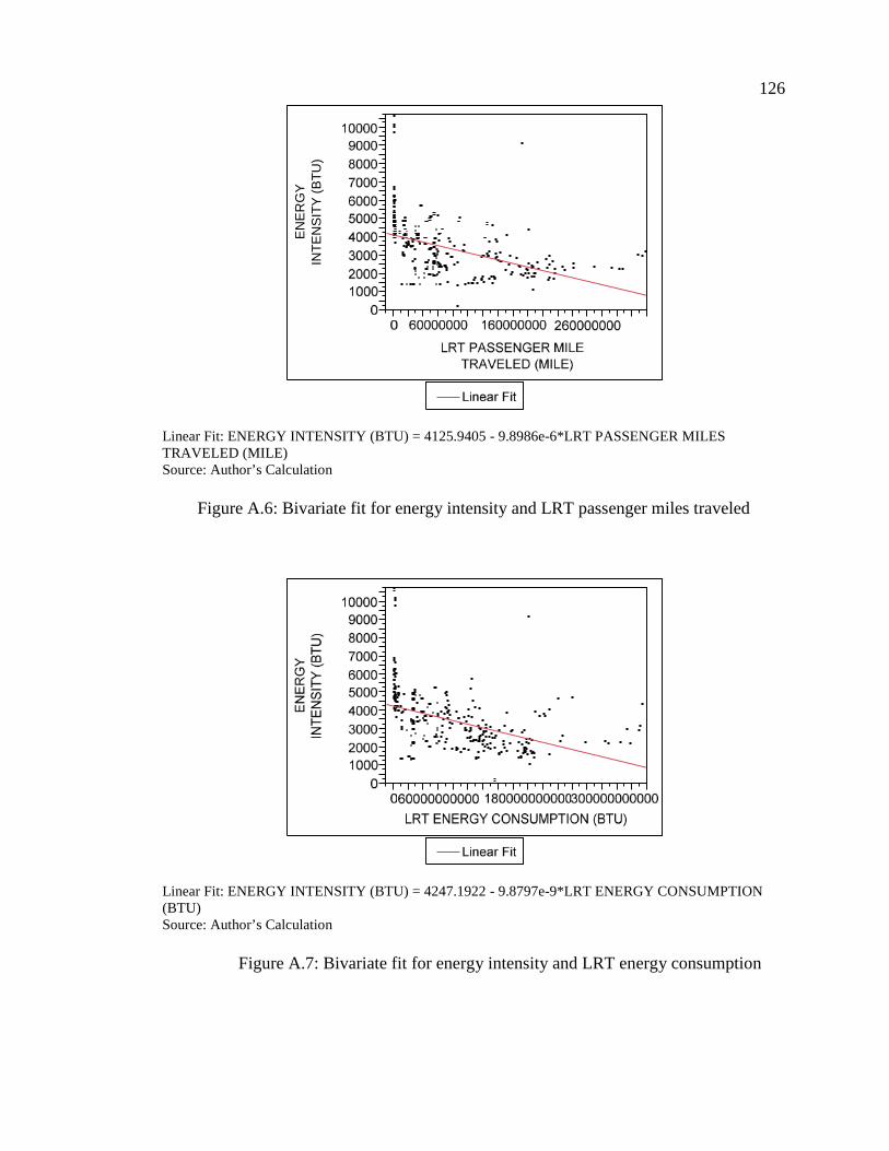
126
Linear Fit: ENERGY INTENSITY (BTU) = 4125.9405 - 9.8986e-6*LRT PASSENGER MILESTRAVELED (MILE)Source: Author’s Calculation
Figure A.6: Bivariate fit for energy intensity and LRT passenger miles traveled
Linear Fit: ENERGY INTENSITY (BTU) = 4247.1922 - 9.8797e-9*LRT ENERGY CONSUMPTION(BTU)Source: Author’s Calculation
Figure A.7: Bivariate fit for energy intensity and LRT energy consumption
ENER
GY
INTE
NSI
TY(B
TU)
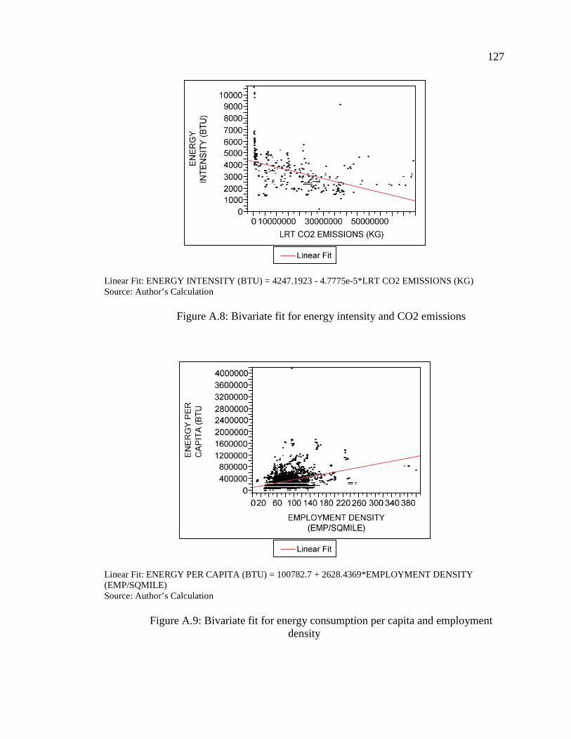
127
Linear Fit: ENERGY INTENSITY (BTU) = 4247.1923 - 4.7775e-5*LRT CO2 EMISSIONS (KG)Source: Author’s Calculation
Figure A.8: Bivariate fit for energy intensity and CO2 emissions
Linear Fit: ENERGY PER CAPITA (BTU) = 100782.7 + 2628.4369*EMPLOYMENT DENSITY(EMP/SQMILE)Source: Author’s Calculation
Figure A.9: Bivariate fit for energy consumption per capita and employmentdensity
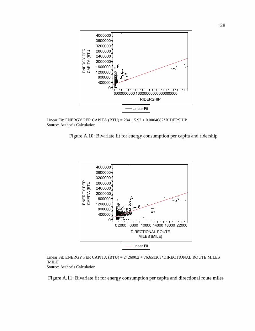
128
Linear Fit: ENERGY PER CAPITA (BTU) = 284115.92 + 0.0004682*RIDERSHIPSource: Author’s Calculation
Figure A.10: Bivariate fit for energy consumption per capita and ridership
Linear Fit: ENERGY PER CAPITA (BTU) = 242600.2 + 76.651203*DIRECTIONAL ROUTE MILES(MILE)Source: Author’s Calculation
Figure A.11: Bivariate fit for energy consumption per capita and directional route miles
ENER
GY
PER
CAP
ITA
(BTU
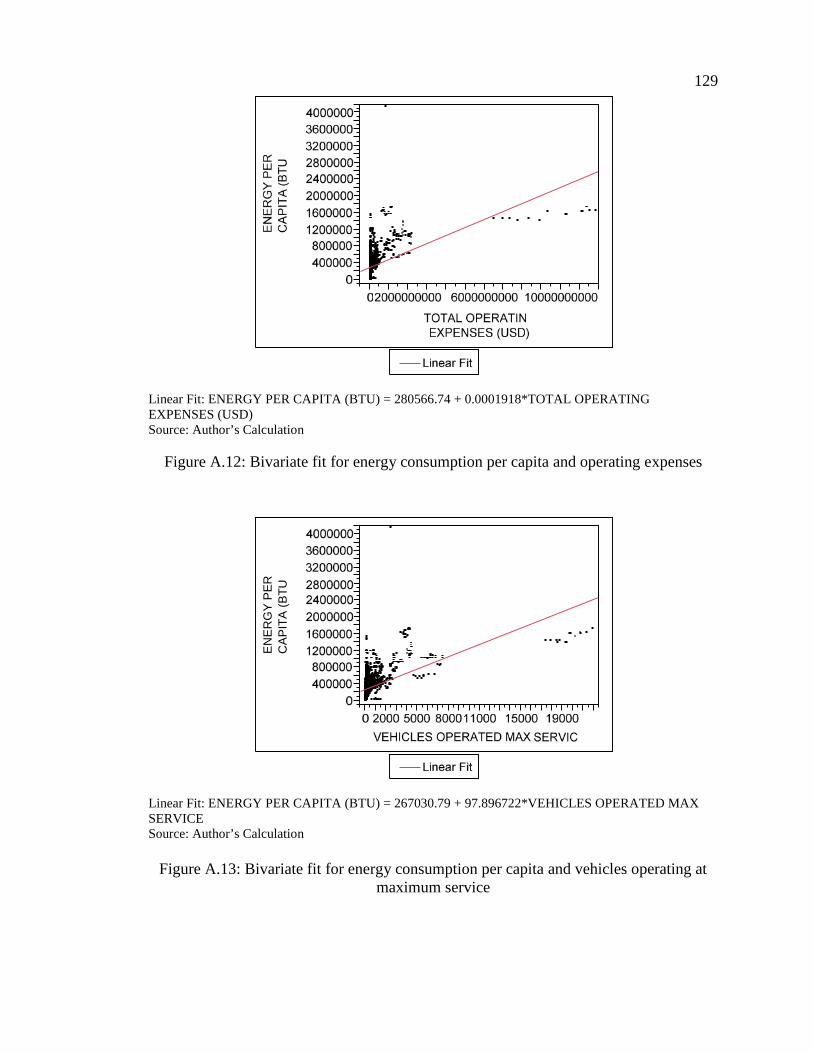
129
Linear Fit: ENERGY PER CAPITA (BTU) = 280566.74 + 0.0001918*TOTAL OPERATINGEXPENSES (USD)Source: Author’s Calculation
Figure A.12: Bivariate fit for energy consumption per capita and operating expenses
Linear Fit: ENERGY PER CAPITA (BTU) = 267030.79 + 97.896722*VEHICLES OPERATED MAXSERVICESource: Author’s Calculation
Figure A.13: Bivariate fit for energy consumption per capita and vehicles operating atmaximum service
ENER
GY
PER
CAP
ITA
(BTU
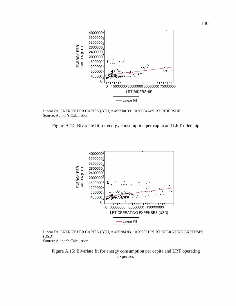
130
Linear Fit: ENERGY PER CAPITA (BTU) = 495500.39 + 0.0080474*LRT RIDERSHIPSource: Author’s Calculation
Figure A.14: Bivariate fit for energy consumption per capita and LRT ridership
Linear Fit: ENERGY PER CAPITA (BTU) = 455284.83 + 0.0039512*LRT OPERATING EXPENSES(USD)Source: Author’s Calculation
Figure A.15: Bivariate fit for energy consumption per capita and LRT operatingexpenses
ENER
GY
PER
CAP
ITA
(BTU
ENER
GY
PER
CAP
ITA
(BTU
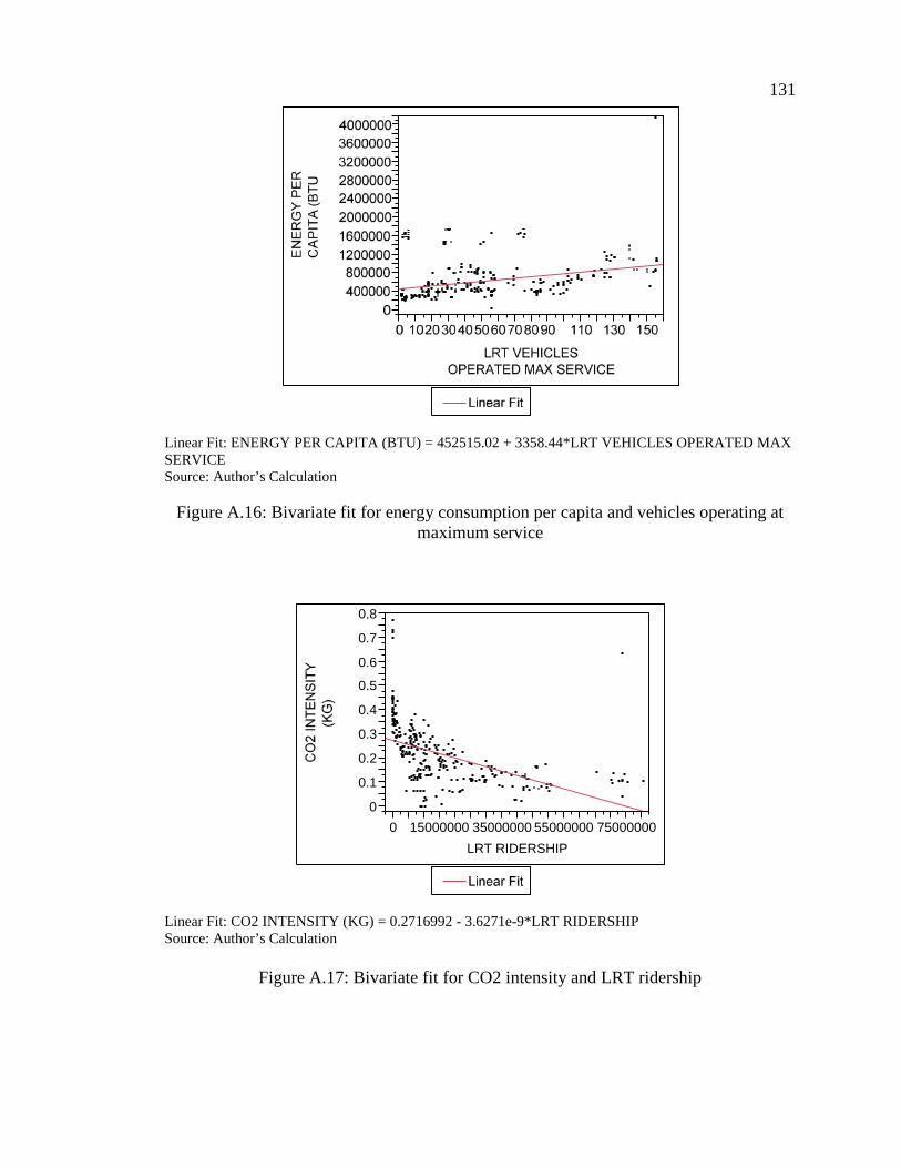
131
Linear Fit: ENERGY PER CAPITA (BTU) = 452515.02 + 3358.44*LRT VEHICLES OPERATED MAXSERVICESource: Author’s Calculation
Figure A.16: Bivariate fit for energy consumption per capita and vehicles operating atmaximum service
Linear Fit: CO2 INTENSITY (KG) = 0.2716992 - 3.6271e-9*LRT RIDERSHIPSource: Author’s Calculation
Figure A.17: Bivariate fit for CO2 intensity and LRT ridership
0
0.1
0.2
0.3
0.4
0.5
0.6
0.7
0.8
0 15000000 35000000 55000000 75000000LRT RIDERSHIP
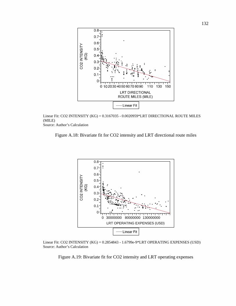
132
Linear Fit: CO2 INTENSITY (KG) = 0.3167035 - 0.0020959*LRT DIRECTIONAL ROUTE MILES(MILE)Source: Author’s Calculation
Figure A.18: Bivariate fit for CO2 intensity and LRT directional route miles
Linear Fit: CO2 INTENSITY (KG) = 0.2854843 - 1.6799e-9*LRT OPERATING EXPENSES (USD)Source: Author’s Calculation
Figure A.19: Bivariate fit for CO2 intensity and LRT operating expenses
0
0.1
0.2
0.3
0.4
0.5
0.6
0.7
0.8
0 30000000 80000000 130000000LRT OPERATING EXPENSES (USD)
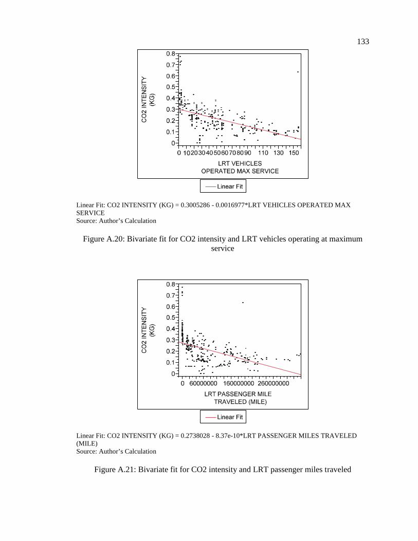
133
Linear Fit: CO2 INTENSITY (KG) = 0.3005286 - 0.0016977*LRT VEHICLES OPERATED MAXSERVICESource: Author’s Calculation
Figure A.20: Bivariate fit for CO2 intensity and LRT vehicles operating at maximumservice
Linear Fit: CO2 INTENSITY (KG) = 0.2738028 - 8.37e-10*LRT PASSENGER MILES TRAVELED(MILE)Source: Author’s Calculation
Figure A.21: Bivariate fit for CO2 intensity and LRT passenger miles traveled
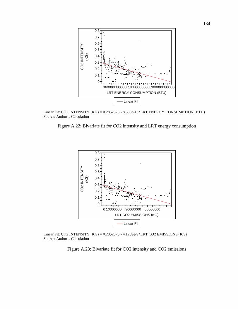
134
Linear Fit: CO2 INTENSITY (KG) = 0.2852573 - 8.538e-13*LRT ENERGY CONSUMPTION (BTU)Source: Author’s Calculation
Figure A.22: Bivariate fit for CO2 intensity and LRT energy consumption
Linear Fit: CO2 INTENSITY (KG) = 0.2852573 - 4.1289e-9*LRT CO2 EMISSIONS (KG)Source: Author’s Calculation
Figure A.23: Bivariate fit for CO2 intensity and CO2 emissions
0
0.1
0.2
0.3
0.4
0.5
0.6
0.7
0.8
060000000000 180000000000300000000000LRT ENERGY CONSUMPTION (BTU)
0
0.1
0.2
0.3
0.4
0.5
0.6
0.7
0.8
0 10000000 30000000 50000000LRT CO2 EMISSIONS (KG)
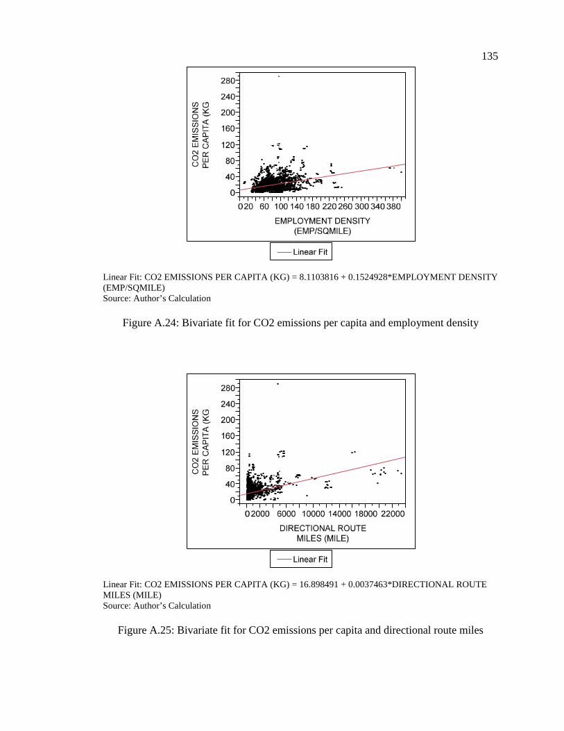
135
Linear Fit: CO2 EMISSIONS PER CAPITA (KG) = 8.1103816 + 0.1524928*EMPLOYMENT DENSITY(EMP/SQMILE)Source: Author’s Calculation
Figure A.24: Bivariate fit for CO2 emissions per capita and employment density
Linear Fit: CO2 EMISSIONS PER CAPITA (KG) = 16.898491 + 0.0037463*DIRECTIONAL ROUTEMILES (MILE)Source: Author’s Calculation
Figure A.25: Bivariate fit for CO2 emissions per capita and directional route miles
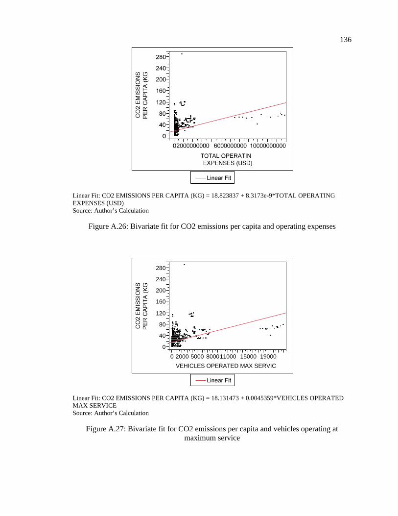
136
Linear Fit: CO2 EMISSIONS PER CAPITA (KG) = 18.823837 + 8.3173e-9*TOTAL OPERATINGEXPENSES (USD)Source: Author’s Calculation
Figure A.26: Bivariate fit for CO2 emissions per capita and operating expenses
Linear Fit: CO2 EMISSIONS PER CAPITA (KG) = 18.131473 + 0.0045359*VEHICLES OPERATEDMAX SERVICESource: Author’s Calculation
Figure A.27: Bivariate fit for CO2 emissions per capita and vehicles operating atmaximum service
0
40
80
120
160
200
240
280
0 2000 5000 800011000 15000 19000VEHICLES OPERATED MAX SERVIC
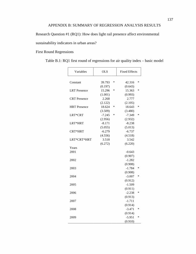
137
APPENDIX B: SUMMARY OF REGRESSION ANALYSIS RESULTS
Research Question #1 (RQ1): How does light rail presence affect environmental
sustainability indicators in urban areas?
First Round Regressions
Table B.1: RQ1 first round of regressions for air quality index – basic model
Variables OLS Fixed Effects
Constant 39.793 * 42.316 *(0.197) (0.643)
LRT Presence 15.296 * 15.363 *(1.001) (0.993)
CRT Presence 2.268 2.777(2.122) (2.105)
HRT Presence 18.624 * 18.643 *(3.509) (3.480)
LRT*CRT -7.245 * -7.349 *(2.956) (2.932)
LRT*HRT -8.171 -8.238(5.055) (5.013)
CRT*HRT -6.279 -6.737(4.556) (4.518)
LRT*CRT*HRT 3.518 3.542(6.272) (6.220)
Years2001 -0.643
(0.907)2002 -1.282
(0.908)2003 -1.784 *
(0.908)2004 -3.007 *
(0.912)2005 -1.509
(0.911)2006 -2.238 *
(0.913)2007 -1.711
(0.914)2008 -3.471 *
(0.914)2009 -5.951 *
(0.910)
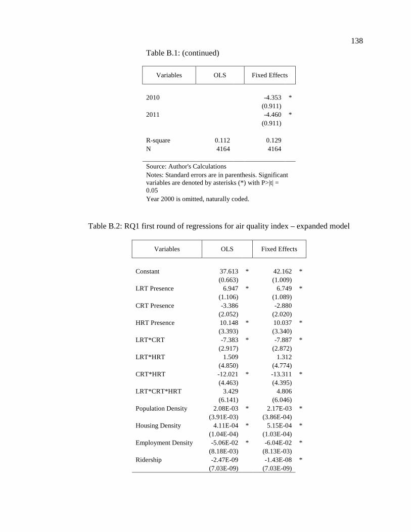
138
Table B.1: (continued)
Variables OLS Fixed Effects
2010 -4.353 *(0.911)
2011 -4.460 *(0.911)
R-square 0.112 0.129N 4164 4164
Source: Author's CalculationsNotes: Standard errors are in parenthesis. Significantvariables are denoted by asterisks (*) with P>|t| =0.05Year 2000 is omitted, naturally coded.
Table B.2: RQ1 first round of regressions for air quality index – expanded model
Variables OLS Fixed Effects
Constant 37.613 * 42.162 *(0.663) (1.009)
LRT Presence 6.947 * 6.749 *(1.106) (1.089)
CRT Presence -3.386 -2.880(2.052) (2.020)
HRT Presence 10.148 * 10.037 *(3.393) (3.340)
LRT*CRT -7.383 * -7.887 *(2.917) (2.872)
LRT*HRT 1.509 1.312(4.850) (4.774)
CRT*HRT -12.021 * -13.311 *(4.463) (4.395)
LRT*CRT*HRT 3.429 4.806(6.141) (6.046)
Population Density 2.08E-03 * 2.17E-03 *(3.91E-03) (3.86E-04)
Housing Density 4.11E-04 * 5.15E-04 *(1.04E-04) (1.03E-04)
Employment Density -5.06E-02 * -6.04E-02 *(8.18E-03) (8.13E-03)
Ridership -2.47E-09 -1.43E-08 *(7.03E-09) (7.03E-09)
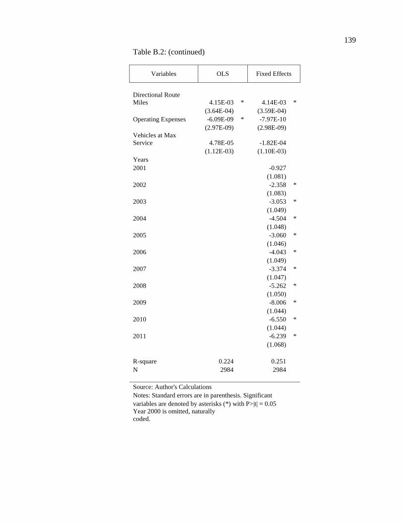
139
Table B.2: (continued)
Variables OLS Fixed Effects
Directional RouteMiles 4.15E-03 * 4.14E-03 *
(3.64E-04) (3.59E-04)Operating Expenses -6.09E-09 * -7.97E-10
(2.97E-09) (2.98E-09)Vehicles at MaxService 4.78E-05 -1.82E-04
(1.12E-03) (1.10E-03)Years2001 -0.927
(1.081)2002 -2.358 *
(1.083)2003 -3.053 *
(1.049)2004 -4.504 *
(1.048)2005 -3.060 *
(1.046)2006 -4.043 *
(1.049)2007 -3.374 *
(1.047)2008 -5.262 *
(1.050)2009 -8.006 *
(1.044)2010 -6.550 *
(1.044)2011 -6.239 *
(1.068)
R-square 0.224 0.251N 2984 2984
Source: Author's CalculationsNotes: Standard errors are in parenthesis. Significantvariables are denoted by asterisks (*) with P>|t| = 0.05Year 2000 is omitted, naturallycoded.
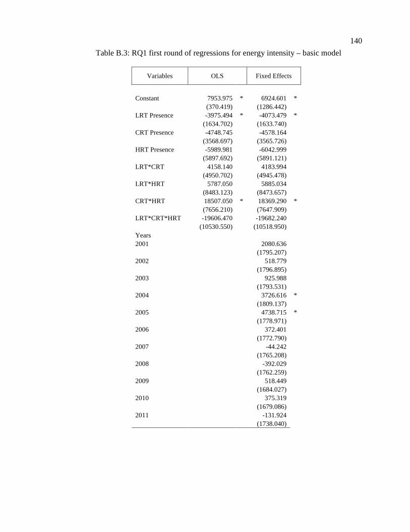
140
Table B.3: RQ1 first round of regressions for energy intensity – basic model
Variables OLS Fixed Effects
Constant 7953.975 * 6924.601 *(370.419) (1286.442)
LRT Presence -3975.494 * -4073.479 *(1634.702) (1633.740)
CRT Presence -4748.745 -4578.164(3568.697) (3565.726)
HRT Presence -5989.981 -6042.999(5897.692) (5891.121)
LRT*CRT 4158.140 4183.994(4950.702) (4945.478)
LRT*HRT 5787.050 5885.034(8483.123) (8473.657)
CRT*HRT 18507.050 * 18369.290 *(7656.210) (7647.909)
LRT*CRT*HRT -19606.470 -19682.240(10530.550) (10518.950)
Years2001 2080.636
(1795.207)2002 518.779
(1796.895)2003 925.988
(1793.531)2004 3726.616 *
(1809.137)2005 4738.715 *
(1778.971)2006 372.401
(1772.790)2007 -44.242
(1765.208)2008 -392.029
(1762.259)2009 518.449
(1684.027)2010 375.319
(1679.086)2011 -131.924
(1738.040)
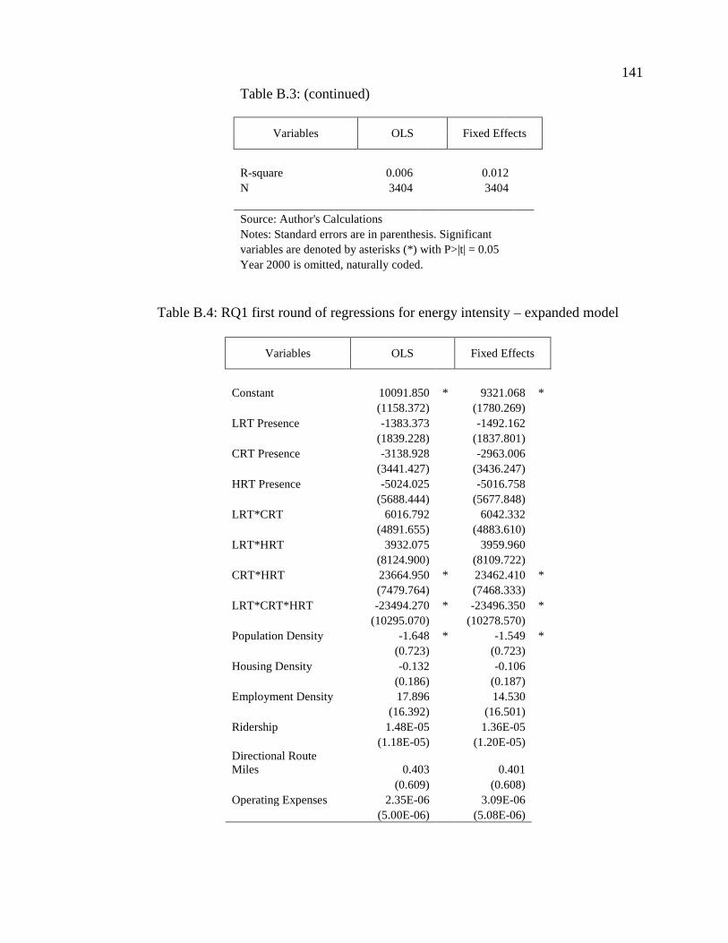
141
Table B.3: (continued)
Variables OLS Fixed Effects
R-square 0.006 0.012N 3404 3404
Source: Author's CalculationsNotes: Standard errors are in parenthesis. Significantvariables are denoted by asterisks (*) with P>|t| = 0.05Year 2000 is omitted, naturally coded.
Table B.4: RQ1 first round of regressions for energy intensity – expanded model
Variables OLS Fixed Effects
Constant 10091.850 * 9321.068 *(1158.372) (1780.269)
LRT Presence -1383.373 -1492.162(1839.228) (1837.801)
CRT Presence -3138.928 -2963.006(3441.427) (3436.247)
HRT Presence -5024.025 -5016.758(5688.444) (5677.848)
LRT*CRT 6016.792 6042.332(4891.655) (4883.610)
LRT*HRT 3932.075 3959.960(8124.900) (8109.722)
CRT*HRT 23664.950 * 23462.410 *(7479.764) (7468.333)
LRT*CRT*HRT -23494.270 * -23496.350 *(10295.070) (10278.570)
Population Density -1.648 * -1.549 *(0.723) (0.723)
Housing Density -0.132 -0.106(0.186) (0.187)
Employment Density 17.896 14.530(16.392) (16.501)
Ridership 1.48E-05 1.36E-05(1.18E-05) (1.20E-05)
Directional RouteMiles 0.403 0.401
(0.609) (0.608)Operating Expenses 2.35E-06 3.09E-06
(5.00E-06) (5.08E-06)
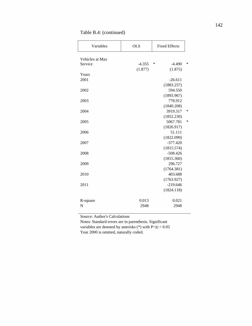
142
Table B.4: (continued)
Variables OLS Fixed Effects
Vehicles at MaxService -4.355 * -4.490 *
(1.877) (1.875)Years2001 -26.611
(1883.257)2002 594.550
(1893.967)2003 778.912
(1840.208)2004 3919.317 *
(1852.230)2005 5067.781 *
(1826.917)2006 51.111
(1822.099)2007 -377.420
(1815.574)2008 -508.426
(1815.360)2009 296.727
(1764.381)2010 403.688
(1763.927)2011 -219.646
(1824.118)
R-square 0.013 0.021N 2948 2948
Source: Author's CalculationsNotes: Standard errors are in parenthesis. Significantvariables are denoted by asterisks (*) with P>|t| = 0.05Year 2000 is omitted, naturally coded.
143
Table B.5: RQ1 first round of regressions for energy consumption per capita – basicmodel
Variables OLS Fixed Effects
Constant 267232.500 * 258120.900 *(7381.518) (25829.560)
LRT Presence 160067.500 * 162715.500(32804.190) (32788.380)
CRT Presence 114451.300 112102.40070585.680 (70550.770)
HRT Presence 158899.200 159475.200(118392.300) (118281.700)
LRT*CRT 253341.600 * 251191.200 *(98626.730) (98540.600)
LRT*HRT -51872.200 -54520.110(170295.600) (170136.300)
CRT*HRT 297337.300 298923.500(153208.600) (153072.700)
LRT*CRT*HRT -213842.300 -210531.700(211044.600) (210847.500)
Years2001 1188.233
(36011.580)2002 92232.010 *
(35944.940)2003 -4582.253
(35879.100)2004 -8181.416
(35751.000)2005 -13748.060
(35563.450)2006 -16904.930
(35473.190)2007 -14209.230
(35324.790)2008 -11455.100
35354.2302009 23796.430
(33751.800)2010 17534.640
(33693.020)2011 36757.260
(34863.020)
R-square 0.097 0.102N 3450 3450
144
Table B.5: (continued)
Source: Author's CalculationsNotes: Standard errors are in parenthesis. Significantvariables are denoted by asterisks (*) with P>|t| = 0.05Year 2000 is omitted, naturally coded.
Table B.6: RQ1 first round of regressions for energy consumption per capita – expandedmodel
Variables OLS Fixed Effects
Constant 133372.700 * 132746.900 *(10815.770) (16625.120)
LRT Presence 40164.020 * 43731.150 *(17212.330) (17171.490)
CRT Presence 54572.560 51697.350(32208.880) (32109.970)
HRT Presence 95031.720 95596.980(53239.440) (53056.460)
LRT*CRT 121137.400 * 119434.000 *(45780.960) (45633.450)
LRT*HRT 44722.420 42914.610(76044.070) (75782.280)
CRT*HRT -58679.240 -53934.120(70002.510) (69786.250)
LRT*CRT*HRT -99055.860 -98065.850(96354.410) (96048.350)
Population Density 25.963 * 23.320 *(6.748) (6.745)
Housing Density 5.928 * 5.167 *(1.739) (1.743)
Employment Density 826.641 * 913.460 *(152.745) (153.540)
Ridership -0.001 * -0.001 *(1.11E-04) (1.12E-04)
Directional RouteMiles -12.024 * -12.244 *
(5.692) (5.680)Operating Expenses 2.50E-05 1.05E-05
(4.68E-05) (4.74E-05)Vehicles at MaxService 205.079 * 207.183 *
(17.565) (17.515)Years2001 1335.766
(17578.070)
145
Table B.6: (continued)
Variables OLS Fixed Effects
2002 17379.030(17677.360)
2003 -9372.000(17149.180)
2004 -14597.170(17073.240)
2005 -19732.230(16994.400)
2006 -22118.480(17011.510)
2007 -18234.400(16951.110)
2008 -14794.880(16963.820)
2009 24853.880(16487.330)
2010 18791.010(16482.970)
2011 32181.670(17045.290)
R-square 0.452 0.457N 2974 2974
Source: Author's CalculationsNotes: Standard errors are in parenthesis. Significantvariables are denoted by asterisks (*) with P>|t| = 0.05Year 2000 is omitted, naturally coded.
Table B.7: RQ1 first round of regressions for CO2 intensity – basic model
Variables OLS Fixed Effects
Constant 0.555 * 0.497 *(0.027) (0.094)
LRT Presence -0.293 * -0.301 *(0.120) (0.120)
CRT Presence -0.341 -0.324(0.262) (0.262)
HRT Presence -0.457 -0.461(0.433) (0.432)
146
Table B.7: (continued)
Variables OLS Fixed Effects
LRT*CRT 0.278 0.280(0.363) (0.363)
LRT*HRT 0.422 0.429(0.623) (0.622)
CRT*HRT 0.975 0.960(0.562) (0.561)
LRT*CRT*HRT -1.029 -1.034(0.773) (0.772)
Years2001 0.150
(0.132)2002 0.032
(0.132)2003 0.066
(0.132)2004 0.263
(0.133)2005 0.338 *
(0.131)2006 0.014
(0.131)2007 -0.022
(0.131)2008 -0.060
(0.131)2009 0.001
(0.124)2010 0.006
(0.124)2011 -0.046
(0.129)
R-square 0.005 0.011N 3336 3336
Source: Author's CalculationsNotes: Standard errors are in parenthesis. Significantvariables are denoted by asterisks (*) with P>|t| = 0.05Year 2000 is omitted, naturally coded.
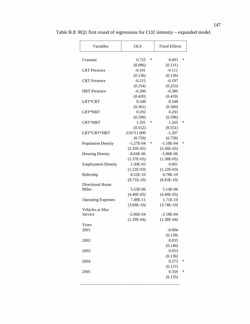
147
Table B.8: RQ1 first round of regressions for CO2 intensity – expanded model
Variables OLS Fixed Effects
Constant 0.725 * 0.693 *(0.086) (0.131)
LRT Presence -0.101 -0.111(0.136) (0.136)
CRT Presence -0.215 -0.197(0.254) (0.253)
HRT Presence -0.390 -0.389(0.420) (0.419)
LRT*CRT 0.349 0.348(0.361) (0.360)
LRT*HRT 0.292 0.293(0.599) (0.598)
CRT*HRT 1.291 * 1.265 *(0.552) (0.551)
LRT*CRT*HRT -216711.000 -1.207(0.759) (0.758)
Population Density -1.27E-04 * -1.18E-04 *(5.35E-05) (5.36E-05)
Housing Density -8.64E-06 -5.86E-06(1.37E-05) (1.38E-05)
Employment Density 1.30E-03 0.001(1.22E-03) (1.22E-03)
Ridership 8.52E-10 6.78E-10(8.71E-10) (8.83E-10)
Directional RouteMiles 5.53E-06 5.14E-06
(4.49E-05) (4.49E-05)Operating Expenses 7.49E-11 1.71E-10
(3.69E-10) (3.74E-10)Vehicles at MaxService -2.06E-04 -2.18E-04
(1.39E-04) (1.38E-04)Years2001 -0.004
(0.139)2002 0.035
(0.140)2003 0.053
(0.136)2004 0.273 *
(0.137)2005 0.359 *
(0.135)
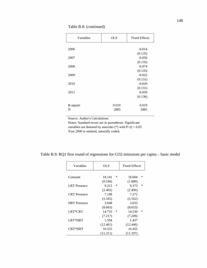
148
Table B.8: (continued)
Variables OLS Fixed Effects
2006 -0.014(0.135)
2007 -0.050(0.135)
2008 -0.074(0.135)
2009 -0.022(0.131)
2010 -0.020(0.131)
2011 -0.059(0.136)
R-square 0.010 0.019N 2885 2885
Source: Author's CalculationsNotes: Standard errors are in parenthesis. Significantvariables are denoted by asterisks (*) with P>|t| = 0.05Year 2000 is omitted, naturally coded.
Table B.9: RQ1 first round of regressions for CO2 emissions per capita – basic model
Variables OLS Fixed Effects
Constant 18.141 * 18.604 *(0.546) (1.889)
LRT Presence 9.215 * 9.373 *(2.402) (2.400)
CRT Presence 7.198 7.272(5.165) (5.162)
HRT Presence 3.048 3.033(8.663) (8.653)
LRT*CRT 14.733 * 14.530 *(7.217) (7.209)
LRT*HRT 1.594 1.437(12.461) (12.446)
CRT*HRT 16.555 16.455(11.211) (11.197)
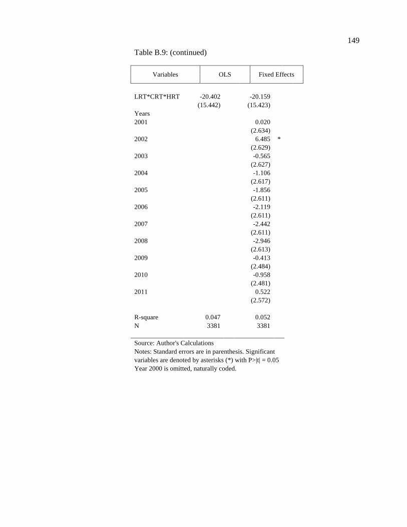
149
Table B.9: (continued)
Variables OLS Fixed Effects
LRT*CRT*HRT -20.402 -20.159(15.442) (15.423)
Years2001 0.020
(2.634)2002 6.485 *
(2.629)2003 -0.565
(2.627)2004 -1.106
(2.617)2005 -1.856
(2.611)2006 -2.119
(2.611)2007 -2.442
(2.611)2008 -2.946
(2.613)2009 -0.413
(2.484)2010 -0.958
(2.481)2011 0.522
(2.572)
R-square 0.047 0.052N 3381 3381
Source: Author's CalculationsNotes: Standard errors are in parenthesis. Significantvariables are denoted by asterisks (*) with P>|t| = 0.05Year 2000 is omitted, naturally coded.
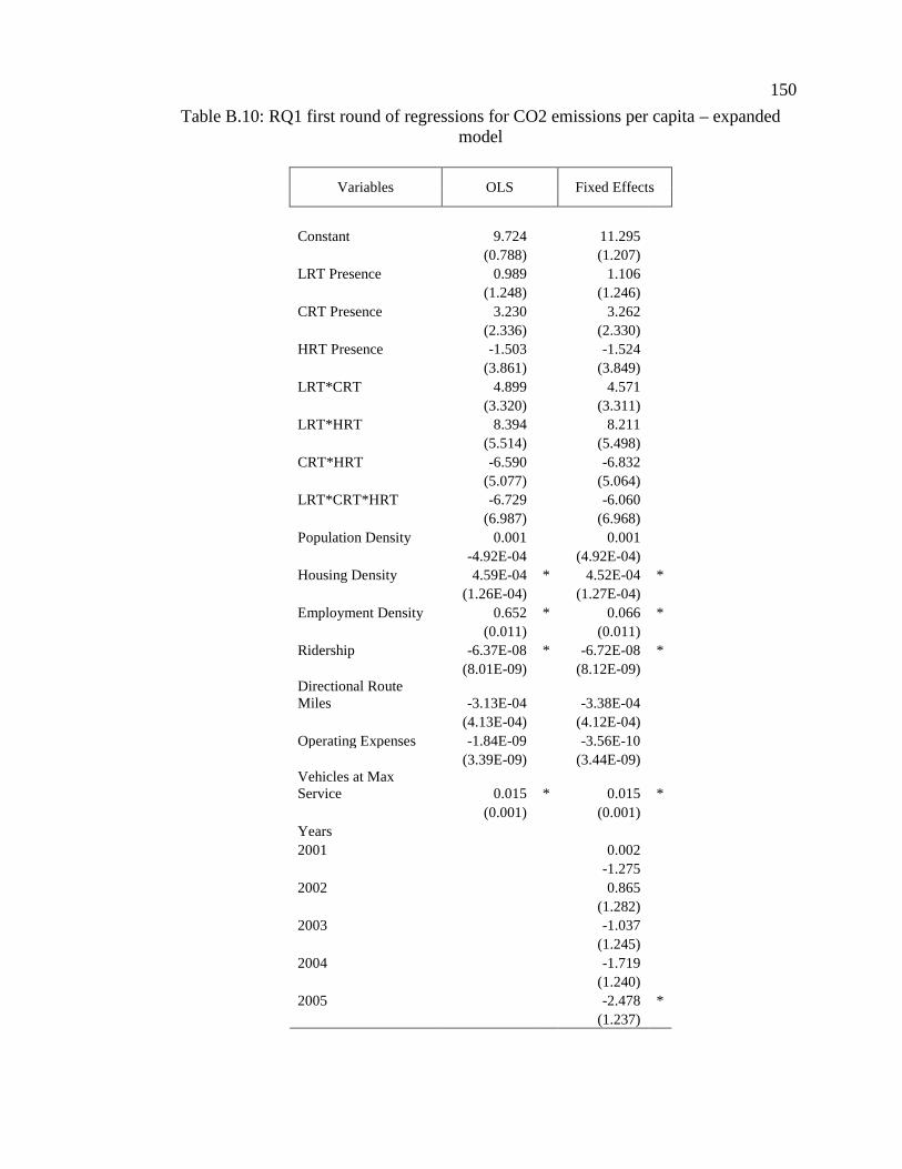
150
Table B.10: RQ1 first round of regressions for CO2 emissions per capita – expandedmodel
Variables OLS Fixed Effects
Constant 9.724 11.295(0.788) (1.207)
LRT Presence 0.989 1.106(1.248) (1.246)
CRT Presence 3.230 3.262(2.336) (2.330)
HRT Presence -1.503 -1.524(3.861) (3.849)
LRT*CRT 4.899 4.571(3.320) (3.311)
LRT*HRT 8.394 8.211(5.514) (5.498)
CRT*HRT -6.590 -6.832(5.077) (5.064)
LRT*CRT*HRT -6.729 -6.060(6.987) (6.968)
Population Density 0.001 0.001-4.92E-04 (4.92E-04)
Housing Density 4.59E-04 * 4.52E-04 *(1.26E-04) (1.27E-04)
Employment Density 0.652 * 0.066 *(0.011) (0.011)
Ridership -6.37E-08 * -6.72E-08 *(8.01E-09) (8.12E-09)
Directional RouteMiles -3.13E-04 -3.38E-04
(4.13E-04) (4.12E-04)Operating Expenses -1.84E-09 -3.56E-10
(3.39E-09) (3.44E-09)Vehicles at MaxService 0.015 * 0.015 *
(0.001) (0.001)Years2001 0.002
-1.2752002 0.865
(1.282)2003 -1.037
(1.245)2004 -1.719
(1.240)2005 -2.478 *
(1.237)
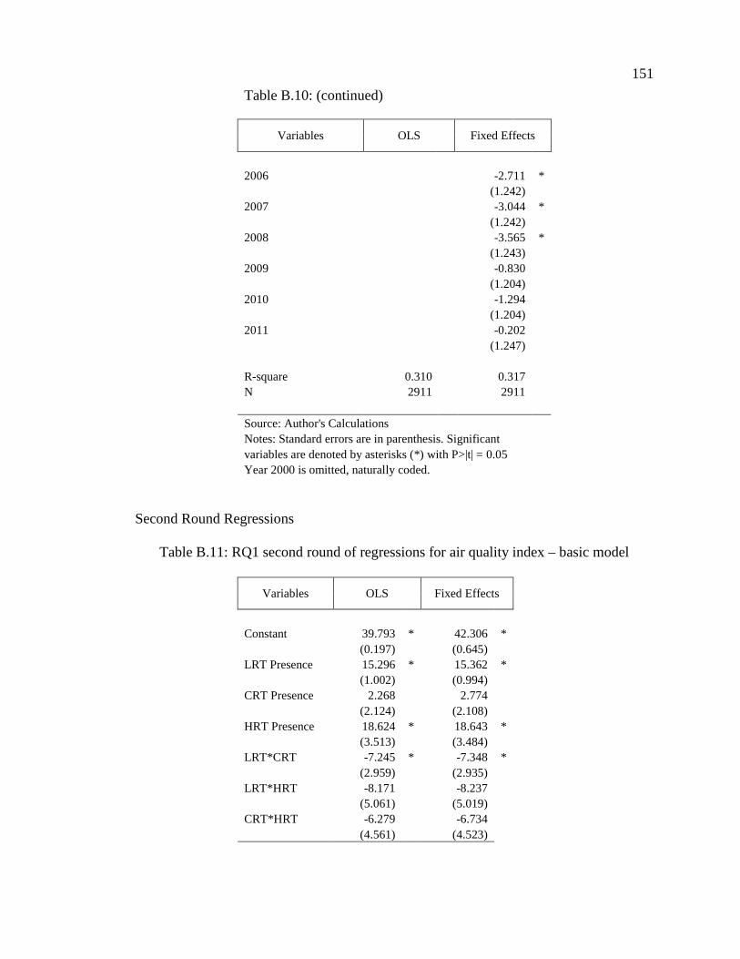
151
Table B.10: (continued)
Variables OLS Fixed Effects
2006 -2.711 *(1.242)
2007 -3.044 *(1.242)
2008 -3.565 *(1.243)
2009 -0.830(1.204)
2010 -1.294(1.204)
2011 -0.202(1.247)
R-square 0.310 0.317N 2911 2911
Source: Author's CalculationsNotes: Standard errors are in parenthesis. Significantvariables are denoted by asterisks (*) with P>|t| = 0.05Year 2000 is omitted, naturally coded.
Second Round Regressions
Table B.11: RQ1 second round of regressions for air quality index – basic model
Variables OLS Fixed Effects
Constant 39.793 * 42.306 *(0.197) (0.645)
LRT Presence 15.296 * 15.362 *(1.002) (0.994)
CRT Presence 2.268 2.774(2.124) (2.108)
HRT Presence 18.624 * 18.643 *(3.513) (3.484)
LRT*CRT -7.245 * -7.348 *(2.959) (2.935)
LRT*HRT -8.171 -8.237(5.061) (5.019)
CRT*HRT -6.279 -6.734(4.561) (4.523)
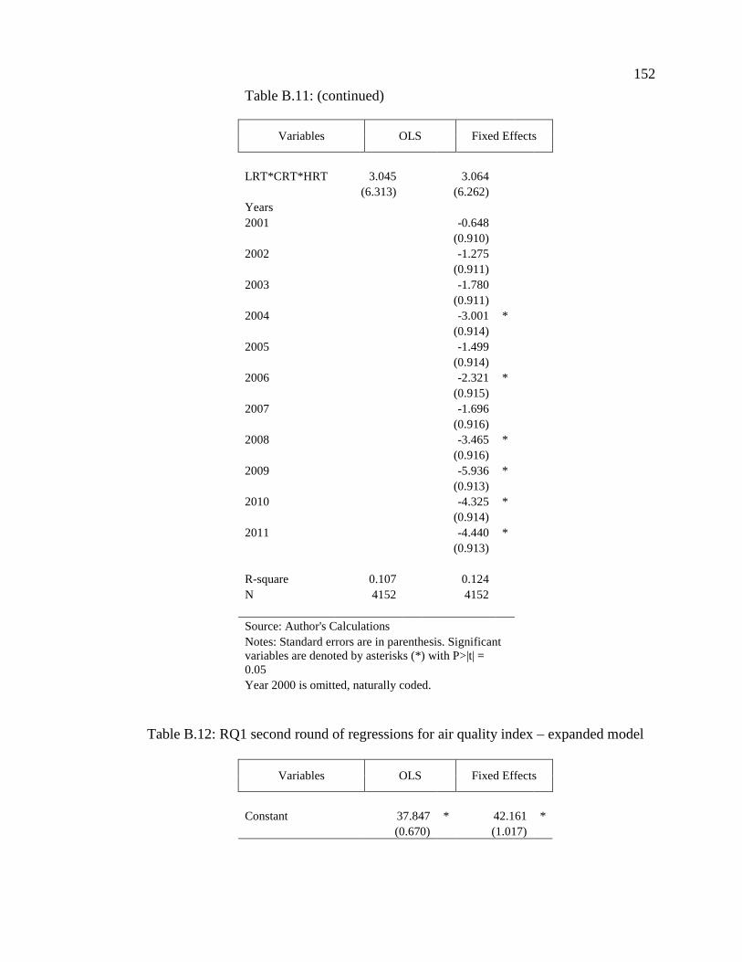
152
Table B.11: (continued)
Variables OLS Fixed Effects
LRT*CRT*HRT 3.045 3.064(6.313) (6.262)
Years2001 -0.648
(0.910)2002 -1.275
(0.911)2003 -1.780
(0.911)2004 -3.001 *
(0.914)2005 -1.499
(0.914)2006 -2.321 *
(0.915)2007 -1.696
(0.916)2008 -3.465 *
(0.916)2009 -5.936 *
(0.913)2010 -4.325 *
(0.914)2011 -4.440 *
(0.913)
R-square 0.107 0.124N 4152 4152
Source: Author's CalculationsNotes: Standard errors are in parenthesis. Significantvariables are denoted by asterisks (*) with P>|t| =0.05Year 2000 is omitted, naturally coded.
Table B.12: RQ1 second round of regressions for air quality index – expanded model
Variables OLS Fixed Effects
Constant 37.847 * 42.161 *(0.670) (1.017)
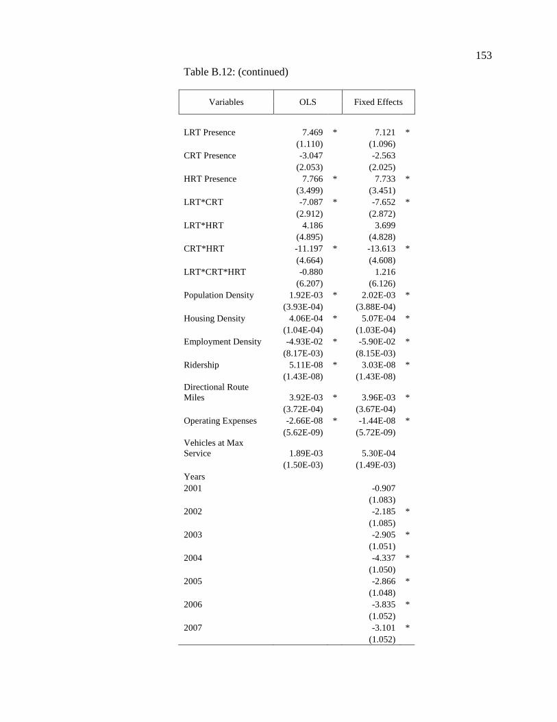
153
Table B.12: (continued)
Variables OLS Fixed Effects
LRT Presence 7.469 * 7.121 *(1.110) (1.096)
CRT Presence -3.047 -2.563(2.053) (2.025)
HRT Presence 7.766 * 7.733 *(3.499) (3.451)
LRT*CRT -7.087 * -7.652 *(2.912) (2.872)
LRT*HRT 4.186 3.699(4.895) (4.828)
CRT*HRT -11.197 * -13.613 *(4.664) (4.608)
LRT*CRT*HRT -0.880 1.216(6.207) (6.126)
Population Density 1.92E-03 * 2.02E-03 *(3.93E-04) (3.88E-04)
Housing Density 4.06E-04 * 5.07E-04 *(1.04E-04) (1.03E-04)
Employment Density -4.93E-02 * -5.90E-02 *(8.17E-03) (8.15E-03)
Ridership 5.11E-08 * 3.03E-08 *(1.43E-08) (1.43E-08)
Directional RouteMiles 3.92E-03 * 3.96E-03 *
(3.72E-04) (3.67E-04)Operating Expenses -2.66E-08 * -1.44E-08 *
(5.62E-09) (5.72E-09)Vehicles at MaxService 1.89E-03 5.30E-04
(1.50E-03) (1.49E-03)Years2001 -0.907
(1.083)2002 -2.185 *
(1.085)2003 -2.905 *
(1.051)2004 -4.337 *
(1.050)2005 -2.866 *
(1.048)2006 -3.835 *
(1.052)2007 -3.101 *
(1.052)
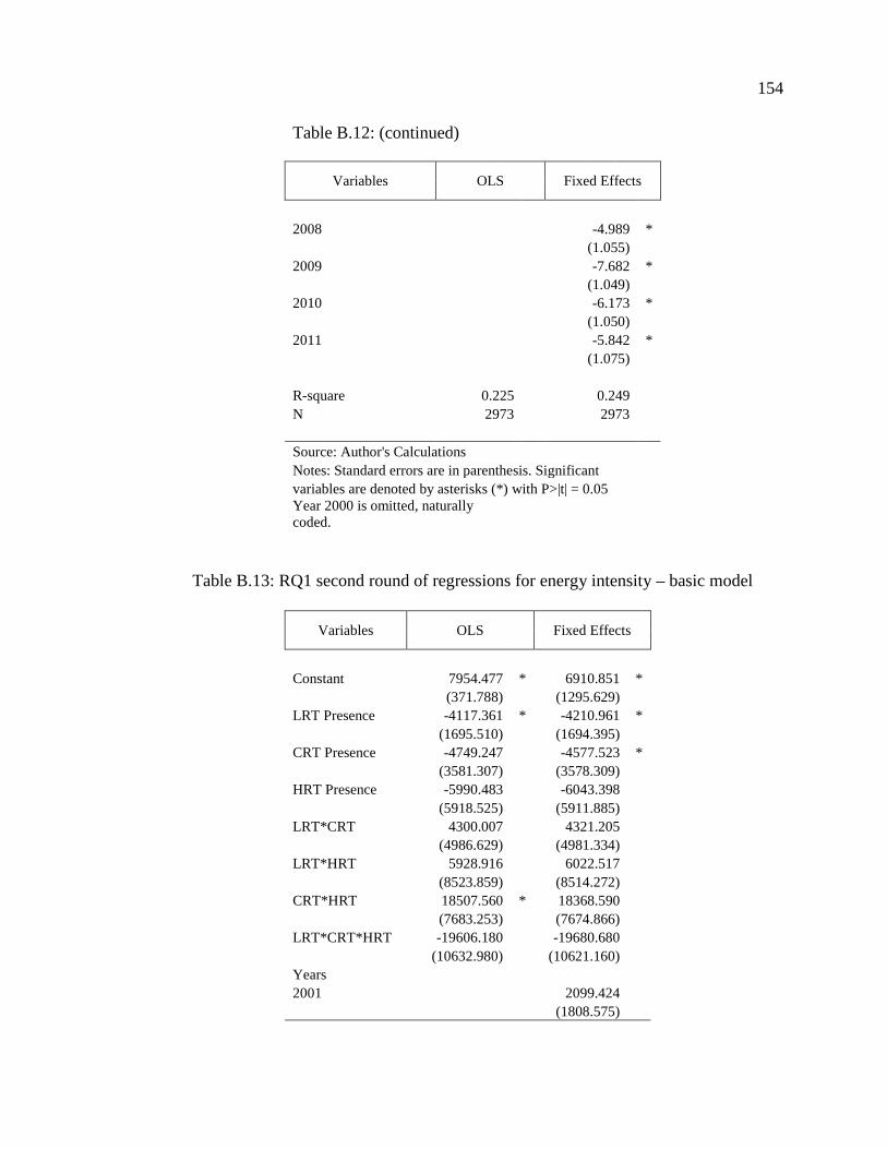
154
Table B.12: (continued)
Variables OLS Fixed Effects
2008 -4.989 *(1.055)
2009 -7.682 *(1.049)
2010 -6.173 *(1.050)
2011 -5.842 *(1.075)
R-square 0.225 0.249N 2973 2973
Source: Author's CalculationsNotes: Standard errors are in parenthesis. Significantvariables are denoted by asterisks (*) with P>|t| = 0.05Year 2000 is omitted, naturallycoded.
Table B.13: RQ1 second round of regressions for energy intensity – basic model
Variables OLS Fixed Effects
Constant 7954.477 * 6910.851 *(371.788) (1295.629)
LRT Presence -4117.361 * -4210.961 *(1695.510) (1694.395)
CRT Presence -4749.247 -4577.523 *(3581.307) (3578.309)
HRT Presence -5990.483 -6043.398(5918.525) (5911.885)
LRT*CRT 4300.007 4321.205(4986.629) (4981.334)
LRT*HRT 5928.916 6022.517(8523.859) (8514.272)
CRT*HRT 18507.560 * 18368.590(7683.253) (7674.866)
LRT*CRT*HRT -19606.180 -19680.680(10632.980) (10621.160)
Years2001 2099.424
(1808.575)
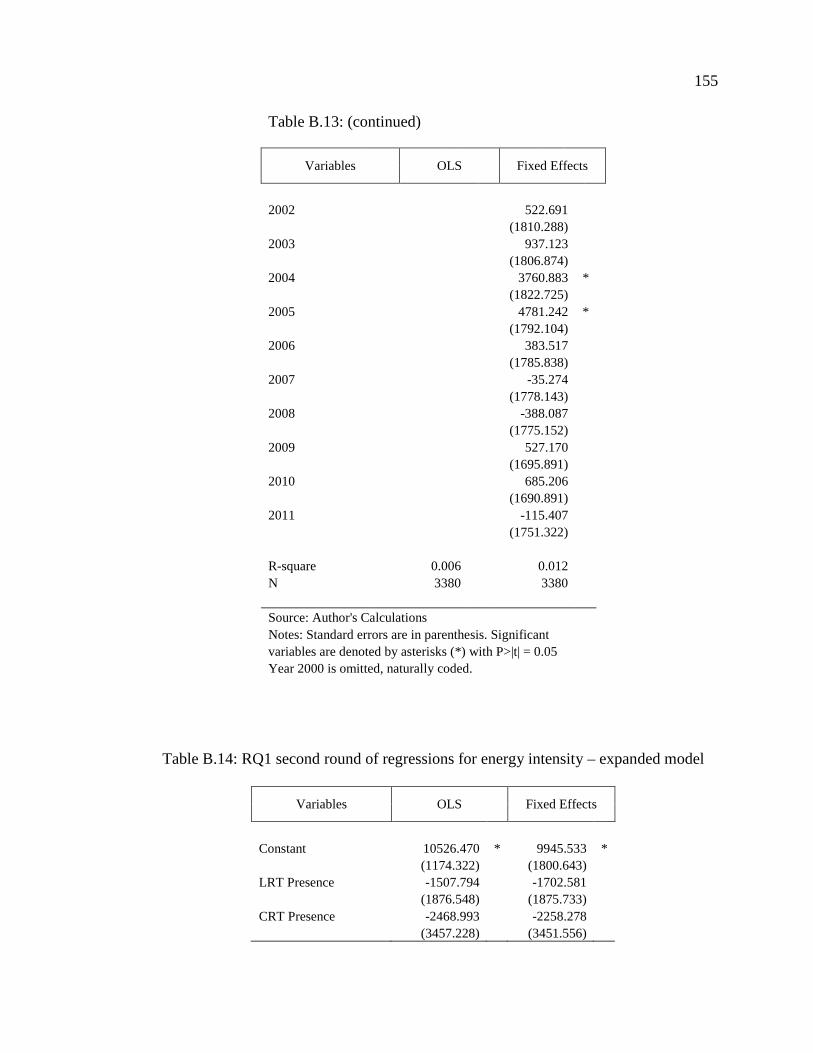
155
Table B.13: (continued)
Variables OLS Fixed Effects
2002 522.691(1810.288)
2003 937.123(1806.874)
2004 3760.883 *(1822.725)
2005 4781.242 *(1792.104)
2006 383.517(1785.838)
2007 -35.274(1778.143)
2008 -388.087(1775.152)
2009 527.170(1695.891)
2010 685.206(1690.891)
2011 -115.407(1751.322)
R-square 0.006 0.012N 3380 3380
Source: Author's CalculationsNotes: Standard errors are in parenthesis. Significantvariables are denoted by asterisks (*) with P>|t| = 0.05Year 2000 is omitted, naturally coded.
Table B.14: RQ1 second round of regressions for energy intensity – expanded model
Variables OLS Fixed Effects
Constant 10526.470 * 9945.533 *(1174.322) (1800.643)
LRT Presence -1507.794 -1702.581(1876.548) (1875.733)
CRT Presence -2468.993 -2258.278(3457.228) (3451.556)
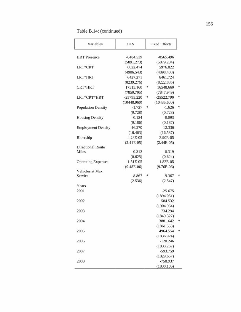
156
Table B.14: (continued)
Variables OLS Fixed Effects
HRT Presence -8484.539 -8565.496(5891.273) (5879.204)
LRT*CRT 6022.474 5976.822(4906.543) (4898.408)
LRT*HRT 6427.271 6461.724(8239.276) (8222.835)
CRT*HRT 17315.160 * 16548.660 *(7850.705) (7847.949)
LRT*CRT*HRT -25795.220 * -25522.790 *(10448.960) (10435.600)
Population Density -1.727 * -1.626 *(0.728) (0.728)
Housing Density -0.124 -0.093(0.186) (0.187)
Employment Density 16.270 12.336(16.463) (16.587)
Ridership 4.28E-05 3.90E-05(2.41E-05) (2.44E-05)
Directional RouteMiles 0.312 0.319
(0.625) (0.624)Operating Expenses 1.51E-05 1.82E-05
(9.48E-06) (9.76E-06)Vehicles at MaxService -8.867 * -9.367 *
(2.536) (2.547)Years2001 -25.675
(1894.051)2002 584.532
(1904.964)2003 734.294
(1849.327)2004 3881.642 *
(1861.553)2005 4964.554 *
(1836.924)2006 -120.246
(1833.267)2007 -593.759
(1829.657)2008 -758.937
(1830.106)
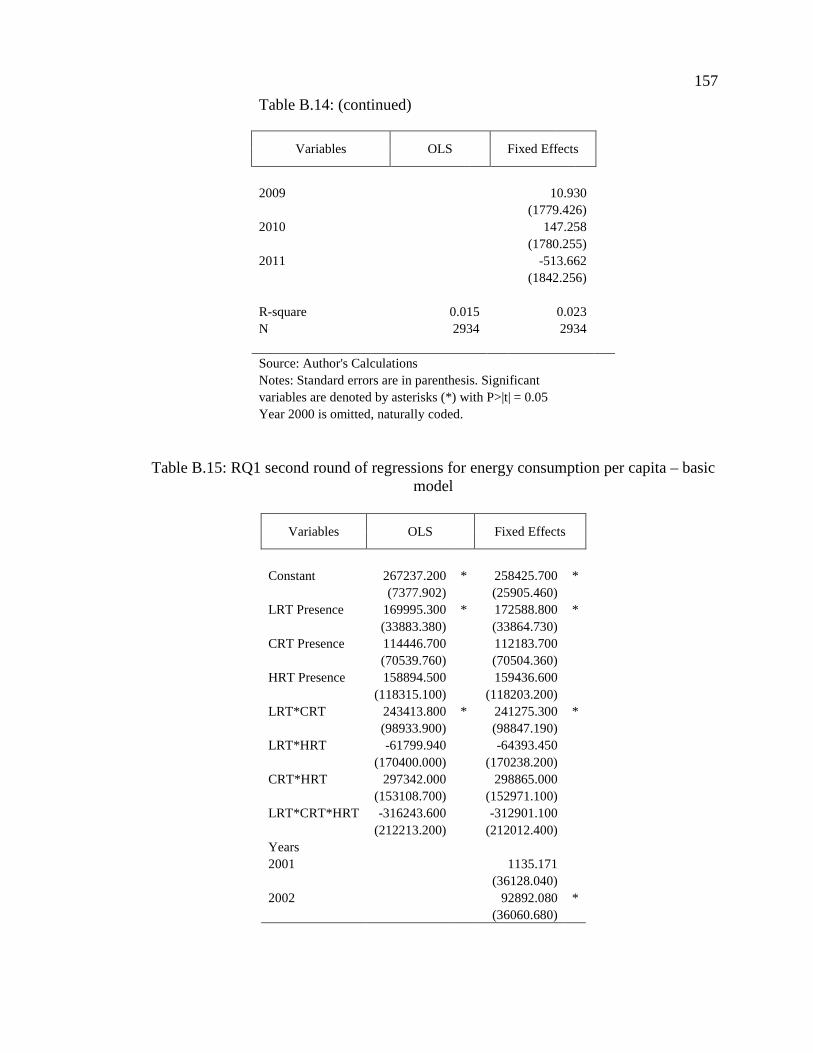
157
Table B.14: (continued)
Variables OLS Fixed Effects
2009 10.930(1779.426)
2010 147.258(1780.255)
2011 -513.662(1842.256)
R-square 0.015 0.023N 2934 2934
Source: Author's CalculationsNotes: Standard errors are in parenthesis. Significantvariables are denoted by asterisks (*) with P>|t| = 0.05Year 2000 is omitted, naturally coded.
Table B.15: RQ1 second round of regressions for energy consumption per capita – basicmodel
Variables OLS Fixed Effects
Constant 267237.200 * 258425.700 *(7377.902) (25905.460)
LRT Presence 169995.300 * 172588.800 *(33883.380) (33864.730)
CRT Presence 114446.700 112183.700(70539.760) (70504.360)
HRT Presence 158894.500 159436.600(118315.100) (118203.200)
LRT*CRT 243413.800 * 241275.300 *(98933.900) (98847.190)
LRT*HRT -61799.940 -64393.450(170400.000) (170238.200)
CRT*HRT 297342.000 298865.000(153108.700) (152971.100)
LRT*CRT*HRT -316243.600 -312901.100(212213.200) (212012.400)
Years2001 1135.171
(36128.040)2002 92892.080 *
(36060.680)
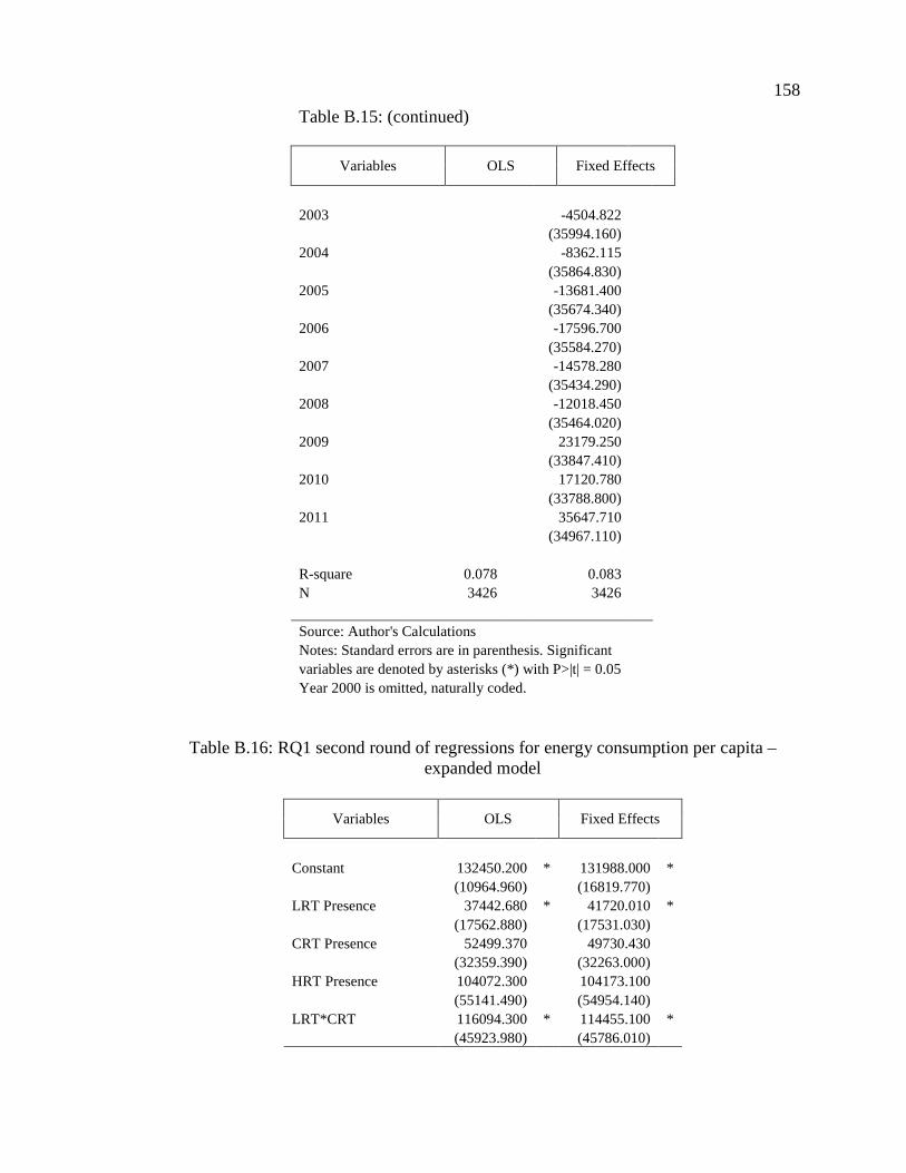
158
Table B.15: (continued)
Variables OLS Fixed Effects
2003 -4504.822(35994.160)
2004 -8362.115(35864.830)
2005 -13681.400(35674.340)
2006 -17596.700(35584.270)
2007 -14578.280(35434.290)
2008 -12018.450(35464.020)
2009 23179.250(33847.410)
2010 17120.780(33788.800)
2011 35647.710(34967.110)
R-square 0.078 0.083N 3426 3426
Source: Author's CalculationsNotes: Standard errors are in parenthesis. Significantvariables are denoted by asterisks (*) with P>|t| = 0.05Year 2000 is omitted, naturally coded.
Table B.16: RQ1 second round of regressions for energy consumption per capita –expanded model
Variables OLS Fixed Effects
Constant 132450.200 * 131988.000 *(10964.960) (16819.770)
LRT Presence 37442.680 * 41720.010 *(17562.880) (17531.030)
CRT Presence 52499.370 49730.430(32359.390) (32263.000)
HRT Presence 104072.300 104173.100(55141.490) (54954.140)
LRT*CRT 116094.300 * 114455.100 *(45923.980) (45786.010)
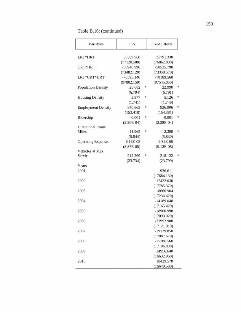
159
Table B.16: (continued)
Variables OLS Fixed Effects
LRT*HRT 36589.960 35791.330(77120.580) (76862.880)
CRT*HRT -58940.990 -50535.790(73482.120) (73358.570)
LRT*CRT*HRT -76595.140 -78189.560(97802.150) (97545.850)
Population Density 25.682 * 22.990 *(6.794) (6.791)
Housing Density 5.877 * 5.126 *(1.741) (1.746)
Employment Density 840.863 * 926.906 *(153.418) (154.381)
Ridership -0.001 * -0.001 *(2.26E-04) (2.28E-04)
Directional RouteMiles -11.965 * -12.390 *
(5.844) (5.830)Operating Expenses 6.16E-05 2.32E-05
(8.87E-05) (9.12E-05)Vehicles at MaxService 212.269 * 218.122 *
(23.734) (23.799)Years2001 936.611
(17684.130)2002 17432.030
(17785.370)2003 -8666.904
(17236.620)2004 -14189.040
(17165.420)2005 -18900.990
(17093.020)2006 -21992.900
(17121.010)2007 -19139.850
(17087.670)2008 -15786.560
(17106.830)2009 24956.640
(16632.960)2010 18429.570
(16640.580)
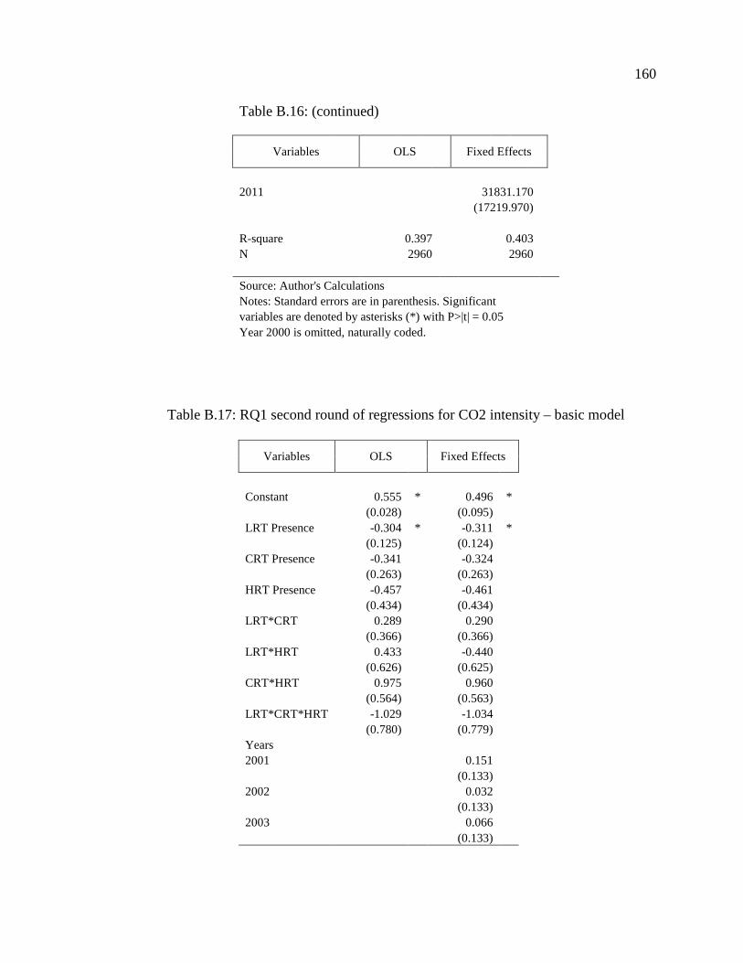
160
Table B.16: (continued)
Variables OLS Fixed Effects
2011 31831.170(17219.970)
R-square 0.397 0.403N 2960 2960
Source: Author's CalculationsNotes: Standard errors are in parenthesis. Significantvariables are denoted by asterisks (*) with P>|t| = 0.05Year 2000 is omitted, naturally coded.
Table B.17: RQ1 second round of regressions for CO2 intensity – basic model
Variables OLS Fixed Effects
Constant 0.555 * 0.496 *(0.028) (0.095)
LRT Presence -0.304 * -0.311 *(0.125) (0.124)
CRT Presence -0.341 -0.324(0.263) (0.263)
HRT Presence -0.457 -0.461(0.434) (0.434)
LRT*CRT 0.289 0.290(0.366) (0.366)
LRT*HRT 0.433 -0.440(0.626) (0.625)
CRT*HRT 0.975 0.960(0.564) (0.563)
LRT*CRT*HRT -1.029 -1.034(0.780) (0.779)
Years2001 0.151
(0.133)2002 0.032
(0.133)2003 0.066
(0.133)
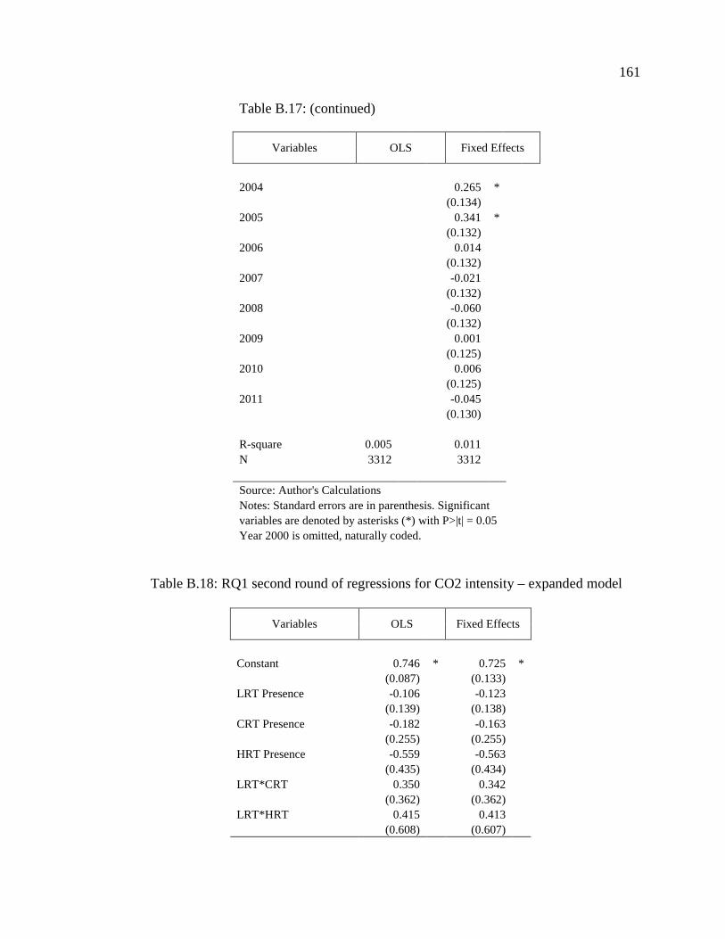
161
Table B.17: (continued)
Variables OLS Fixed Effects
2004 0.265 *(0.134)
2005 0.341 *(0.132)
2006 0.014(0.132)
2007 -0.021(0.132)
2008 -0.060(0.132)
2009 0.001(0.125)
2010 0.006(0.125)
2011 -0.045(0.130)
R-square 0.005 0.011N 3312 3312
Source: Author's CalculationsNotes: Standard errors are in parenthesis. Significantvariables are denoted by asterisks (*) with P>|t| = 0.05Year 2000 is omitted, naturally coded.
Table B.18: RQ1 second round of regressions for CO2 intensity – expanded model
Variables OLS Fixed Effects
Constant 0.746 * 0.725 *(0.087) (0.133)
LRT Presence -0.106 -0.123(0.139) (0.138)
CRT Presence -0.182 -0.163(0.255) (0.255)
HRT Presence -0.559 -0.563(0.435) (0.434)
LRT*CRT 0.350 0.342(0.362) (0.362)
LRT*HRT 0.415 0.413(0.608) (0.607)
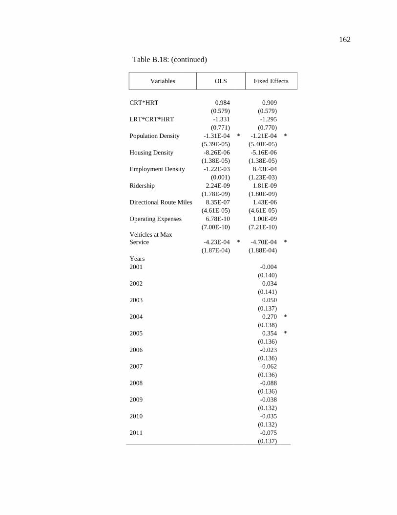
162
Table B.18: (continued)
Variables OLS Fixed Effects
CRT*HRT 0.984 0.909(0.579) (0.579)
LRT*CRT*HRT -1.331 -1.295(0.771) (0.770)
Population Density -1.31E-04 * -1.21E-04 *(5.39E-05) (5.40E-05)
Housing Density -8.26E-06 -5.16E-06(1.38E-05) (1.38E-05)
Employment Density -1.22E-03 8.43E-04(0.001) (1.23E-03)
Ridership 2.24E-09 1.81E-09(1.78E-09) (1.80E-09)
Directional Route Miles 8.35E-07 1.43E-06(4.61E-05) (4.61E-05)
Operating Expenses 6.78E-10 1.00E-09(7.00E-10) (7.21E-10)
Vehicles at MaxService -4.23E-04 * -4.70E-04 *
(1.87E-04) (1.88E-04)Years2001 -0.004
(0.140)2002 0.034
(0.141)2003 0.050
(0.137)2004 0.270 *
(0.138)2005 0.354 *
(0.136)2006 -0.023
(0.136)2007 -0.062
(0.136)2008 -0.088
(0.136)2009 -0.038
(0.132)2010 -0.035
(0.132)2011 -0.075
(0.137)
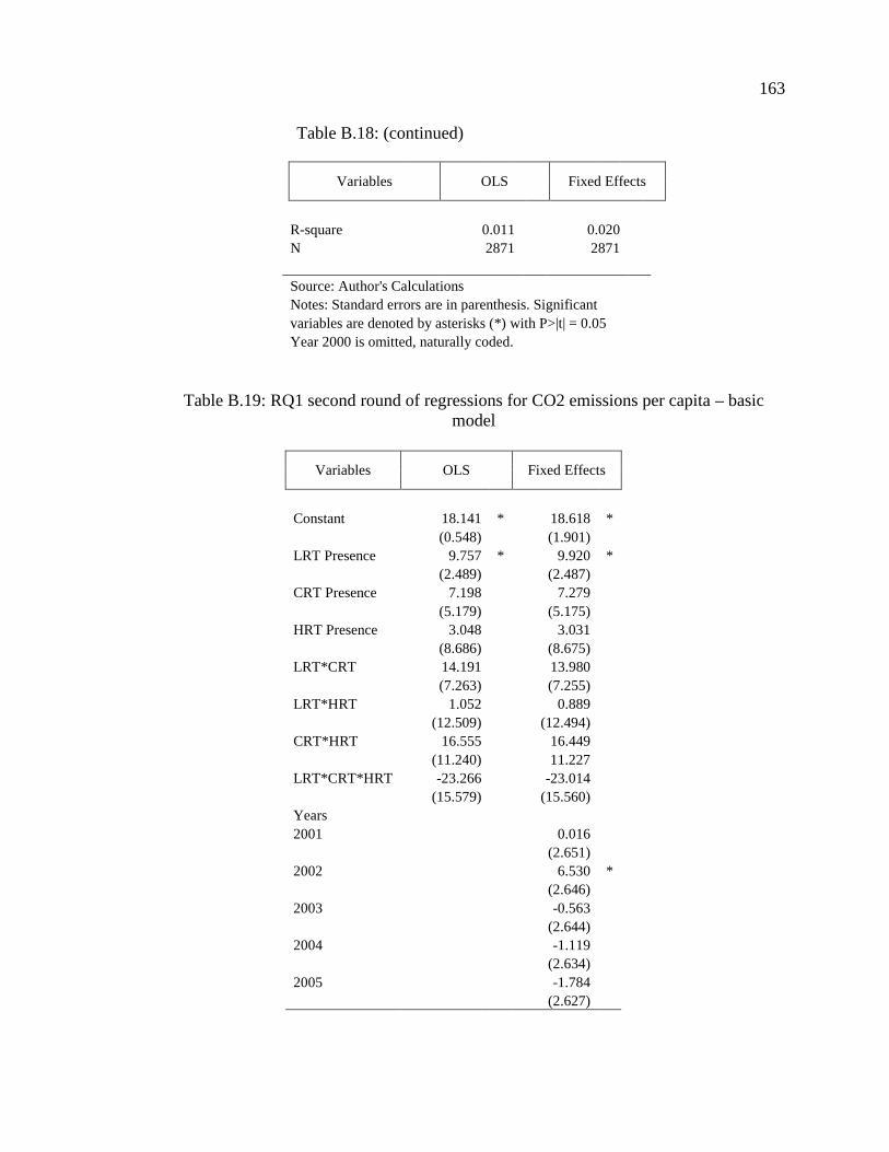
163
Table B.18: (continued)
Variables OLS Fixed Effects
R-square 0.011 0.020N 2871 2871
Source: Author's CalculationsNotes: Standard errors are in parenthesis. Significantvariables are denoted by asterisks (*) with P>|t| = 0.05Year 2000 is omitted, naturally coded.
Table B.19: RQ1 second round of regressions for CO2 emissions per capita – basicmodel
Variables OLS Fixed Effects
Constant 18.141 * 18.618 *(0.548) (1.901)
LRT Presence 9.757 * 9.920 *(2.489) (2.487)
CRT Presence 7.198 7.279(5.179) (5.175)
HRT Presence 3.048 3.031(8.686) (8.675)
LRT*CRT 14.191 13.980(7.263) (7.255)
LRT*HRT 1.052 0.889(12.509) (12.494)
CRT*HRT 16.555 16.449(11.240) 11.227
LRT*CRT*HRT -23.266 -23.014(15.579) (15.560)
Years2001 0.016
(2.651)2002 6.530 *
(2.646)2003 -0.563
(2.644)2004 -1.119
(2.634)2005 -1.784
(2.627)
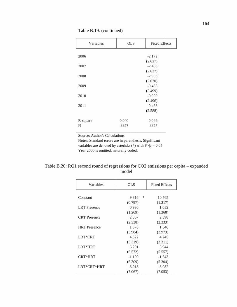
164
Table B.19: (continued)
Variables OLS Fixed Effects
2006 -2.172(2.627)
2007 -2.463(2.627)
2008 -2.983(2.630)
2009 -0.455(2.499)
2010 -0.990(2.496)
2011 0.463(2.588)
R-square 0.040 0.046N 3357 3357
Source: Author's CalculationsNotes: Standard errors are in parenthesis. Significantvariables are denoted by asterisks (*) with P>|t| = 0.05Year 2000 is omitted, naturally coded.
Table B.20: RQ1 second round of regressions for CO2 emissions per capita – expandedmodel
Variables OLS Fixed Effects
Constant 9.316 * 10.765(0.797) (1.217)
LRT Presence 0.930 1.052(1.269) (1.268)
CRT Presence 2.567 2.598(2.338) (2.333)
HRT Presence 1.678 1.646(3.984) (3.973)
LRT*CRT 4.622 4.245(3.319) (3.311)
LRT*HRT 6.201 5.944(5.572) (5.557)
CRT*HRT -1.100 -1.643(5.309) (5.304)
LRT*CRT*HRT -3.918 -3.082(7.067) (7.053)
165
Table B.20: (continued)
Variables OLS Fixed Effects
Population Density 0.001 0.001(4.93E-04) (4.93E-04)
Housing Density 4.47E-04 * 4.38E-04 *(1.26E-04) (1.26E-04)
Employment Density 0.068 * 6.95E-02 *(0.011) (1.12E-02)
Ridership -9.28E-08 * -9.79E-08 *(1.63E-08) (1.65E-08)
Directional RouteMiles -2.65E-04 -2.84E-04
(4.23E-04) (4.22E-04)Operating Expenses -1.34E-08 * -1.04E-08
(6.41E-09) (6.60E-09)Vehicles at MaxService 0.020 * 0.020 *
(0.002) (0.002)Years2001 (0.029)
-1.2792002 0.880
(1.286)2003 -0.947
(1.247)2004 -1.633
(1.242)2005 -2.243
(1.240)2006 -2.582 *
(1.246)2007 -2.943 *
(1.248)2008 -3.447 *
(1.250)2009 -0.612
(1.210)2010 -1.130
(1.212)2011 0.005
(1.255)
R-square 0.293 0.300N 2897 2897
Source: Author's CalculationsNotes: Standard errors are in parenthesis. Significant
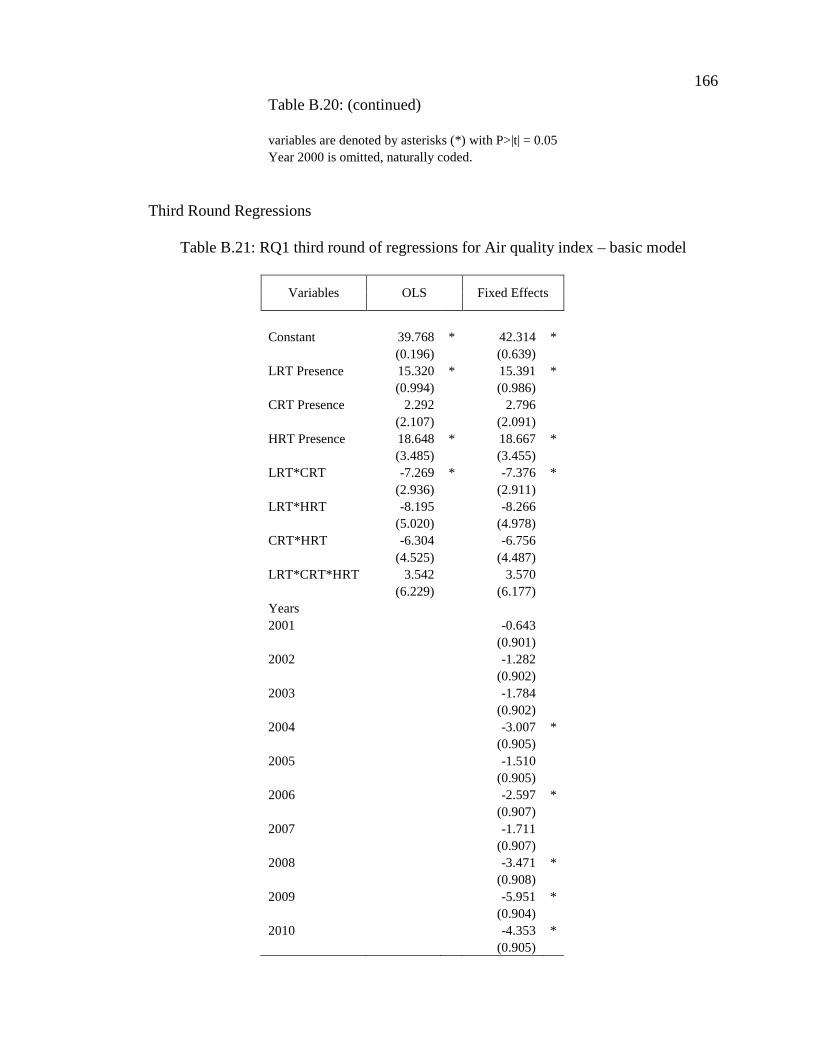
166
Table B.20: (continued)
variables are denoted by asterisks (*) with P>|t| = 0.05Year 2000 is omitted, naturally coded.
Third Round Regressions
Table B.21: RQ1 third round of regressions for Air quality index – basic model
Variables OLS Fixed Effects
Constant 39.768 * 42.314 *(0.196) (0.639)
LRT Presence 15.320 * 15.391 *(0.994) (0.986)
CRT Presence 2.292 2.796(2.107) (2.091)
HRT Presence 18.648 * 18.667 *(3.485) (3.455)
LRT*CRT -7.269 * -7.376 *(2.936) (2.911)
LRT*HRT -8.195 -8.266(5.020) (4.978)
CRT*HRT -6.304 -6.756(4.525) (4.487)
LRT*CRT*HRT 3.542 3.570(6.229) (6.177)
Years2001 -0.643
(0.901)2002 -1.282
(0.902)2003 -1.784
(0.902)2004 -3.007 *
(0.905)2005 -1.510
(0.905)2006 -2.597 *
(0.907)2007 -1.711
(0.907)2008 -3.471 *
(0.908)2009 -5.951 *
(0.904)2010 -4.353 *
(0.905)
167
Table B.21: (continued)
Variables OLS Fixed Effects
2011 -4.461 *(0.904)
R-square 0.114 0.131N 4163 4163
Source: Author's CalculationsNotes: Standard errors are in parenthesis. Significantvariables are denoted by asterisks (*) with P>|t| =0.05Year 2000 is omitted, naturally coded.
Table B.22: RQ1 third round of regressions for Air quality index – expanded model
Variables OLS Fixed Effects
Constant 37.677 * 42.252 *(0.658) (1.000)
LRT Presence 7.183 * 6.992 *(1.097) (1.080)
CRT Presence -3.234 -2.735(2.035) (2.003)
HRT Presence 10.340 * 10.230 *(3.365) (3.311)
LRT*CRT -7.268 * -7.778 *(2.893) (2.847)
LRT*HRT 1.268 1.063(4.810) (4.733)
CRT*HRT -11.711 * -12.997 *(4.426) (4.357)
LRT*CRT*HRT 3.204 4.593(6.090) (5.994)
Population Density 2.03E-03 * 0.002 *(3.88E-04) (3.82E-04)
Housing Density 4.06E-04 * 5.10E-04 *(1.03E-04) (1.02E-04)
Employment Density -4.99E-02 * -5.96E-02 *(8.11E-03) (8.06E-03)
Ridership -1.47E-09 -1.33E-08(6.98E-09) (6.97E-09)
168
Table B.22: (continued)
Variables OLS Fixed Effects
Directional RouteMiles 4.11E-03 * 0.004 *
(3.61E-04) (3.56E-04)Operating Expenses -5.94E-09 * -6.34E-10
(2.95E-09) (2.95E-09)Vehicles at MaxService -1.91E-04 -4.17E-04
(1.11E-03) (1.09E-03)Years2001 -0.924
(1.072)2002 -2.349 *
(1.074)2003 -3.048 *
(1.040)2004 -4.503 *
(1.039)2005 -3.060 *
(1.037)2006 -4.363 *
(1.041)2007 -3.375 *
(1.038)2008 -5.262 *
(1.041)2009 -8.005 *
(1.035)2010 -6.548 *
(1.035)2011 -6.228 *
(1.059)
R-square 0.225 0.252N 2983 2983
Source: Author's CalculationsNotes: Standard errors are in parenthesis. Significantvariables are denoted by asterisks (*) with P>|t| = 0.05Year 2000 is omitted, naturallycoded.
169
Table B.23: RQ1 third round of regressions for energy intensity – basic model
Variables OLS Fixed Effects
Constant 7692.739 * 6894.451 *(274.370) (952.719)
LRT Presence -3714.259 * -3777.576 *(1210.450) (1209.949)
CRT Presence -4487.509 -4372.512(2642.482) (2640.724)
HRT Presence -5728.746 -5770.721(4367.002) (4362.875)
LRT*CRT 3896.905 3905.765(3665.797) (3662.549)
LRT*HRT -5525.815 5589.132(6281.405) (6275.458)
CRT*HRT 18245.820 * 18157.020 *(5669.111) (5663.920)
LRT*CRT*HRT -19345.230 * -19393.940 *(7797.442) (7790.164)
Years2001 2081.672
(1329.501)2002 519.703
(1330.751)2003 926.009
(1328.260)2004 3723.239 *
(1339.817)2005 1803.800
(1318.648)2006 396.144
(1314.042)2007 -45.129
(1307.285)2008 -393.486
(1305.101)2009 521.795
(1247.163)2010 678.462
(1243.504)2011 -129.040
(1287.730)
R-square 0.011 0.016N 3402 3402
Source: Author's CalculationsNotes: Standard errors are in parenthesis. Significant
170
Table B.23: (continued)
variables are denoted by asterisks (*) with P>|t| = 0.05Year 2000 is omitted, naturally coded.
Table B.24: RQ1 third round of regressions for energy intensity – expanded model
Variables OLS Fixed Effects
Constant 9667.907 * 9194.244 *(750.664) (1153.070)
LRT Presence -1450.665 -1524.430(1192.280) (1190.825)
CRT Presence -3081.763 -2964.880(2229.984) (2225.563)
HRT Presence -4953.795 -4952.418(3685.915) (3677.306)
LRT*CRT 5760.457 5758.913(3169.571) (3162.852)
LRT*HRT 3899.155 3908.427(5264.614) (5252.296)
CRT*HRT 23044.740 * 22899.620 *(4846.716) (4837.017)
LRT*CRT*HRT -23047.130 * -23009.380 *(6670.729) (6656.872)
Population Density -1.349 * -1.292 *(0.468) (0.469)
Housing Density -0.085 -0.068(0.120) (0.121)
Employment Density 10.084 7.856(10.622) (10.689)
Ridership 1.31E-05 1.20E-05(7.65E-06) (7.75E-06)
Directional RouteMiles 0.545 0.543
(0.394) (0.394)Operating Expenses 3.03E-06 0.000
(3.24E-06) (3.29E-06)Vehicles at MaxService -4.503 * -4.603 *
(1.219) (1.215)Years2001 -33.121
(1219.668)2002 570.572
(1226.605)2003 767.408
(1191.788)
171
Table B.24: (continued)
Variables OLS Fixed Effects
2004 3913.087 *(119.574)
2005 1808.940(1184.289)
2006 59.748(1181.154)
2007 -383.077(1175.834)
2008 -529.288(1175.696)
2009 261.751(1142.680)
2010 359.844(1142.386)
2011 -281.811(1181.369)
R-square 0.028 0.036N 2946 2946
Source: Author's CalculationsNotes: Standard errors are in parenthesis. Significantvariables are denoted by asterisks (*) with P>|t| = 0.05Year 2000 is omitted, naturally coded.
Table B.25: RQ1 third round of regressions for energy consumption per capita – basicmodel
Variables OLS Fixed Effects
Constant 260444.100 * 257383.000 *(3560.743) (12440.050)
LRT Presence 166856.000 * 169198.200 *(15816.960) (15792.010)
CRT Presence 121239.800 * 117454.400 *(34033.130) (33978.780)
HRT Presence 165687.600 * 166771.200 *(57083.060) (56966.980)
172
Table B.25: (continued)
Variables OLS Fixed Effects
LRT*CRT 246553.000 * 245328.500 *(47553.100) (47459.280)
LRT*HRT -58660.640 -61002.820(82108.280) (81941.150)
CRT*HRT 290548.900 * 293392.900 *(73869.760) (73722.950)
LRT*CRT*HRT -207053.800 * -204397.400 *(101755.400) (101548.500)
Years2001 1216.290
(17343.910)2002 12893.120
(17327.800)2003 -4567.841
(17280.100)2004 -8204.168
(17218.400)2005 -14070.250
(17142.890)2006 -16139.850
(17099.150)2007 -14213.400
(17013.130)2008 -11482.910
(17027.310)2009 23882.120
(16255.550)2010 17610.750
(16227.540)2011 36806.640 *
(16790.730)
R-square 0.322 0.327N 3447 3447
Source: Author's CalculationsNotes: Standard errors are in parenthesis. Significantvariables are denoted by asterisks (*) with P>|t| = 0.05Year 2000 is omitted, naturally coded.
173
Table B.26: RQ1 third round of regressions for energy consumption per capita –expanded model
Variables OLS Fixed Effects
Constant 132961.200 * 132222.800 *(10809.460) (16615.920)
LRT Presence 38854.330 * 42452.380 *(17208.040) (17169.090)
CRT Presence 53722.810 50914.570(32187.570) (32091.150)
HRT Presence 93992.970 94611.610(53202.820) (53024.190)
LRT*CRT 120506.300 * 118870.800 *(45748.710) (45604.850)
LRT*HRT 46023.540 44179.800(75991.190) (75735.720)
CRT*HRT -60421.910 -55611.620(69955.610) (69745.090)
LRT*CRT*HRT -97810.330 -96942.670(96286.370) (95988.030)
Population Density 26.332 * 23.705 *(6.745) (6.742)
Housing Density 5.951 * 5.194 *(1.738) (1.742)
Employment Density 821.157 * 907.495 *(152.658) (153.465)
Ridership -0.001 * -0.001 *(1.10E-04) (1.12E-04)
Directional RouteMiles -11.801 * -12.023 *
(5.689) (5.677)Operating Expenses 2.43E-05 0.000
(4.67E-05) (4.74E-05)Vehicles at MaxService 206.337 * 208.347 *
(17.560) (17.511)Years2001 1322.548
(17566.830)2002 17334.950
(17666.060)2003 -9395.155
(17135.210)2004 -14593.260
(17062.320)2005 -20084.240
(16998.920)
174
Table B.26: (continued)
Variables OLS Fixed Effects
2006 -20402.500(17016.290)
2007 -18210.440(16940.270)
2008 -14781.390(16952.970)
2009 24853.450(16476.780)
2010 18785.750(16472.420)
2011 32120.240(17034.410)
R-square 0.452 0.458N 2972 2972
Source: Author's CalculationsNotes: Standard errors are in parenthesis. Significantvariables are denoted by asterisks (*) with P>|t| = 0.05Year 2000 is omitted, naturally coded.
Table B.27: RQ1 third round of regressions for CO2 intensity – basic model
Variables OLS Fixed Effects
Constant 0.535 * 0.495 *(0.020) (0.069)
LRT Presence -0.274 * -0.278 *(0.088) (0.088)
CRT Presence -0.321 -0.308(0.193) (0.193)
HRT Presence -0.438 -0.441(0.319) (0.318)
LRT*CRT -0.259 0.259(0.268) (0.267)
LRT*HRT 0.403 -0.407(0.458) (0.458)
CRT*HRT 0.955 * 0.945 *(0.414) (0.413)
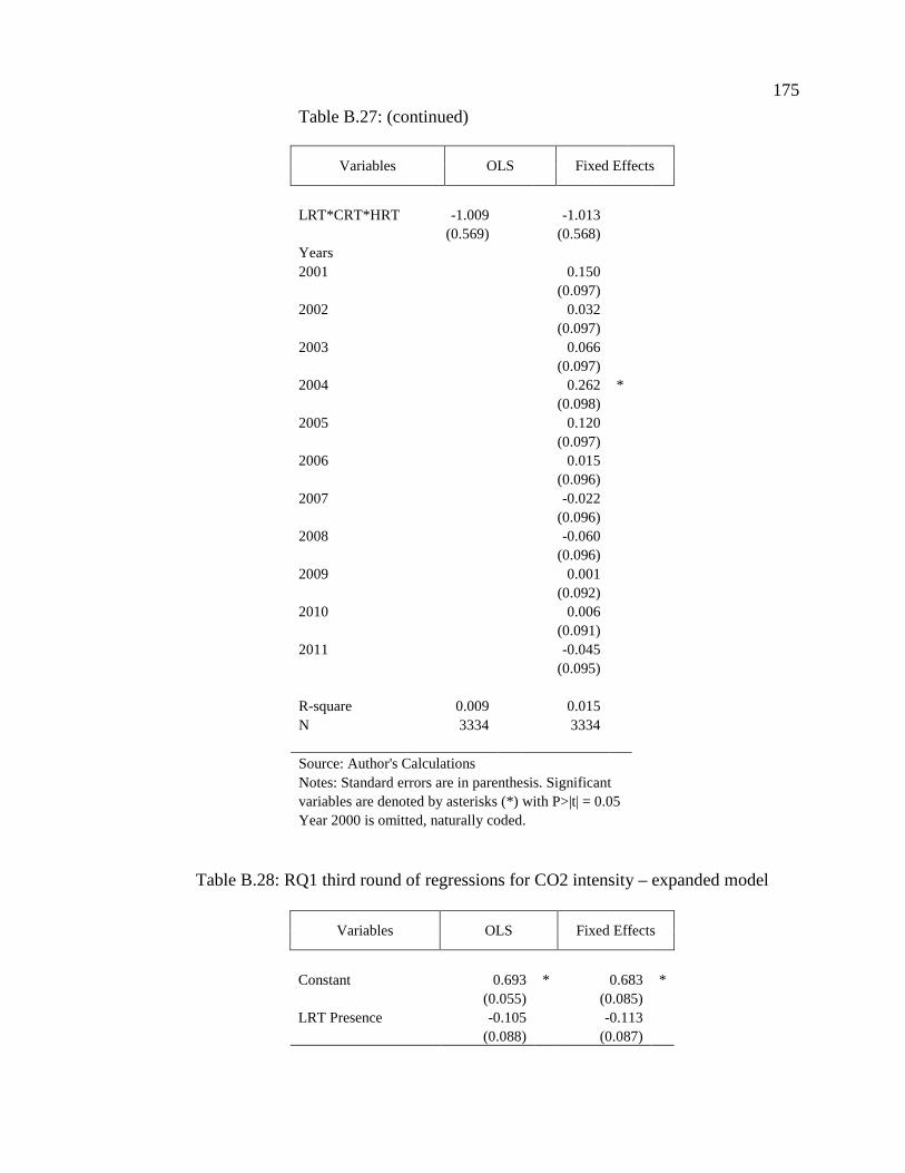
175
Table B.27: (continued)
Variables OLS Fixed Effects
LRT*CRT*HRT -1.009 -1.013(0.569) (0.568)
Years2001 0.150
(0.097)2002 0.032
(0.097)2003 0.066
(0.097)2004 0.262 *
(0.098)2005 0.120
(0.097)2006 0.015
(0.096)2007 -0.022
(0.096)2008 -0.060
(0.096)2009 0.001
(0.092)2010 0.006
(0.091)2011 -0.045
(0.095)
R-square 0.009 0.015N 3334 3334
Source: Author's CalculationsNotes: Standard errors are in parenthesis. Significantvariables are denoted by asterisks (*) with P>|t| = 0.05Year 2000 is omitted, naturally coded.
Table B.28: RQ1 third round of regressions for CO2 intensity – expanded model
Variables OLS Fixed Effects
Constant 0.693 * 0.683 *(0.055) (0.085)
LRT Presence -0.105 -0.113(0.088) (0.087)
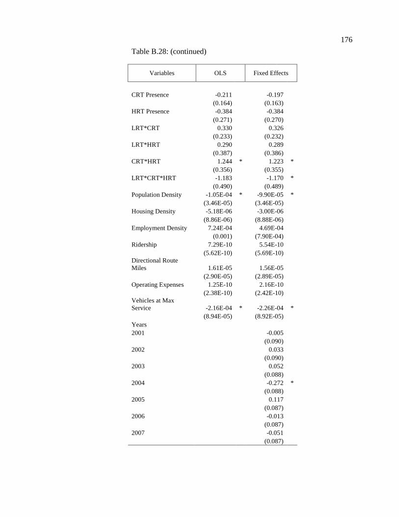
176
Table B.28: (continued)
Variables OLS Fixed Effects
CRT Presence -0.211 -0.197(0.164) (0.163)
HRT Presence -0.384 -0.384(0.271) (0.270)
LRT*CRT 0.330 0.326(0.233) (0.232)
LRT*HRT 0.290 0.289(0.387) (0.386)
CRT*HRT 1.244 * 1.223 *(0.356) (0.355)
LRT*CRT*HRT -1.183 -1.170 *(0.490) (0.489)
Population Density -1.05E-04 * -9.90E-05 *(3.46E-05) (3.46E-05)
Housing Density -5.18E-06 -3.00E-06(8.86E-06) (8.88E-06)
Employment Density 7.24E-04 4.69E-04(0.001) (7.90E-04)
Ridership 7.29E-10 5.54E-10(5.62E-10) (5.69E-10)
Directional RouteMiles 1.61E-05 1.56E-05
(2.90E-05) (2.89E-05)Operating Expenses 1.25E-10 2.16E-10
(2.38E-10) (2.42E-10)Vehicles at MaxService -2.16E-04 * -2.26E-04 *
(8.94E-05) (8.92E-05)Years2001 -0.005
(0.090)2002 0.033
(0.090)2003 0.052
(0.088)2004 -0.272 *
(0.088)2005 0.117
(0.087)2006 -0.013
(0.087)2007 -0.051
(0.087)
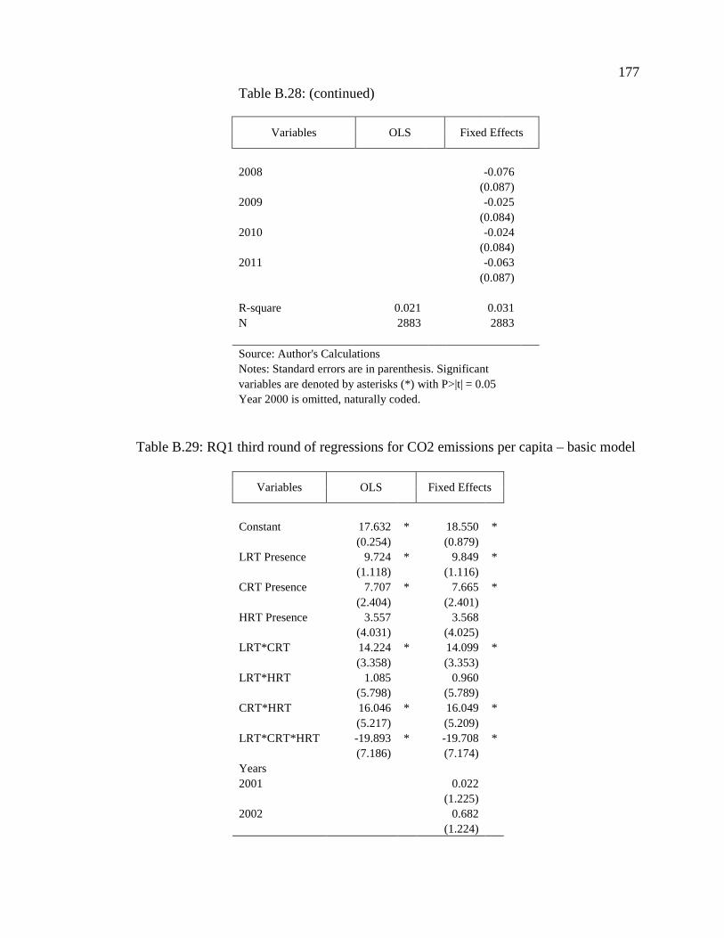
177
Table B.28: (continued)
Variables OLS Fixed Effects
2008 -0.076(0.087)
2009 -0.025(0.084)
2010 -0.024(0.084)
2011 -0.063(0.087)
R-square 0.021 0.031N 2883 2883
Source: Author's CalculationsNotes: Standard errors are in parenthesis. Significantvariables are denoted by asterisks (*) with P>|t| = 0.05Year 2000 is omitted, naturally coded.
Table B.29: RQ1 third round of regressions for CO2 emissions per capita – basic model
Variables OLS Fixed Effects
Constant 17.632 * 18.550 *(0.254) (0.879)
LRT Presence 9.724 * 9.849 *(1.118) (1.116)
CRT Presence 7.707 * 7.665 *(2.404) (2.401)
HRT Presence 3.557 3.568(4.031) (4.025)
LRT*CRT 14.224 * 14.099 *(3.358) (3.353)
LRT*HRT 1.085 0.960(5.798) (5.789)
CRT*HRT 16.046 * 16.049 *(5.217) (5.209)
LRT*CRT*HRT -19.893 * -19.708 *(7.186) (7.174)
Years2001 0.022
(1.225)2002 0.682
(1.224)
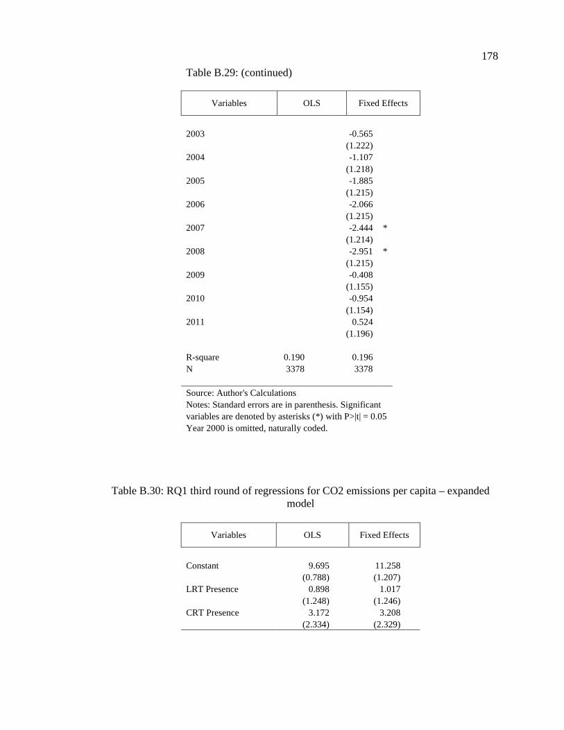
178
Table B.29: (continued)
Variables OLS Fixed Effects
2003 -0.565(1.222)
2004 -1.107(1.218)
2005 -1.885(1.215)
2006 -2.066(1.215)
2007 -2.444 *(1.214)
2008 -2.951 *(1.215)
2009 -0.408(1.155)
2010 -0.954(1.154)
2011 0.524(1.196)
R-square 0.190 0.196N 3378 3378
Source: Author's CalculationsNotes: Standard errors are in parenthesis. Significantvariables are denoted by asterisks (*) with P>|t| = 0.05Year 2000 is omitted, naturally coded.
Table B.30: RQ1 third round of regressions for CO2 emissions per capita – expandedmodel
Variables OLS Fixed Effects
Constant 9.695 11.258(0.788) (1.207)
LRT Presence 0.898 1.017(1.248) (1.246)
CRT Presence 3.172 3.208(2.334) (2.329)
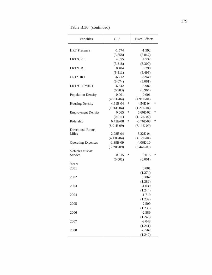
179
Table B.30: (continued)
Variables OLS Fixed Effects
HRT Presence -1.574 -1.592(3.858) (3.847)
LRT*CRT 4.855 4.532(3.318) (3.309)
LRT*HRT 8.484 8.298(5.511) (5.495)
CRT*HRT -6.712 -6.949(5.074) (5.061)
LRT*CRT*HRT -6.642 -5.982(6.983) (6.964)
Population Density 0.001 0.001(4.91E-04) (4.91E-04)
Housing Density 4.61E-04 * 4.54E-04 *(1.26E-04) (1.27E-04)
Employment Density 0.065 * 6.60E-02 *(0.011) (1.12E-02)
Ridership 6.41E-08 * -6.76E-08 *(8.01E-09) (8.11E-09)
Directional RouteMiles -2.98E-04 -3.22E-04
(4.13E-04) (4.12E-04)Operating Expenses -1.89E-09 -4.06E-10
(3.39E-09) (3.44E-09)Vehicles at MaxService 0.015 * 0.015 *
(0.001) (0.001)Years2001 0.001
(1.274)2002 0.862
(1.282)2003 -1.039
(1.244)2004 -1.719
(1.239)2005 -2.509
(1.238)2006 -2.589
(1.243)2007 -3.043
(1.241)2008 -3.562
(1.242)
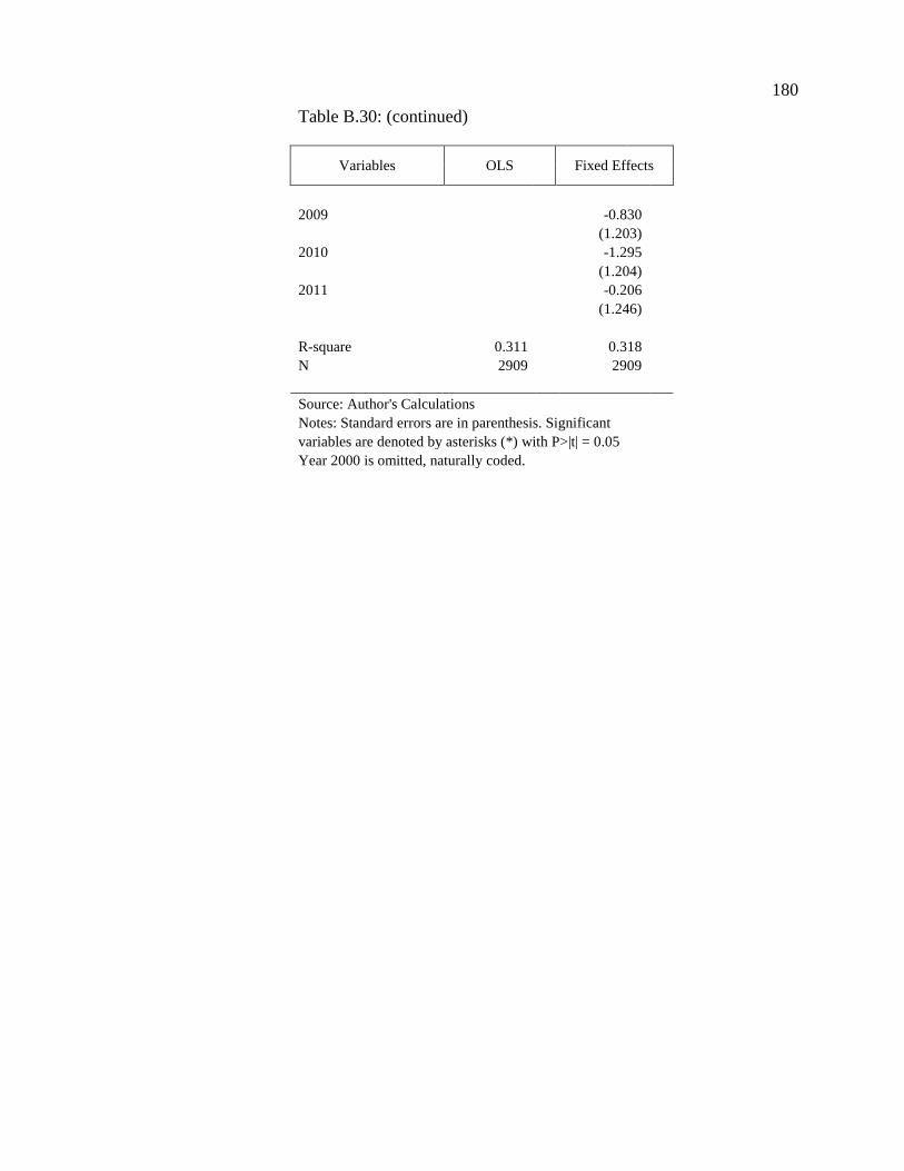
180
Table B.30: (continued)
Variables OLS Fixed Effects
2009 -0.830(1.203)
2010 -1.295(1.204)
2011 -0.206(1.246)
R-square 0.311 0.318N 2909 2909
Source: Author's CalculationsNotes: Standard errors are in parenthesis. Significantvariables are denoted by asterisks (*) with P>|t| = 0.05Year 2000 is omitted, naturally coded.
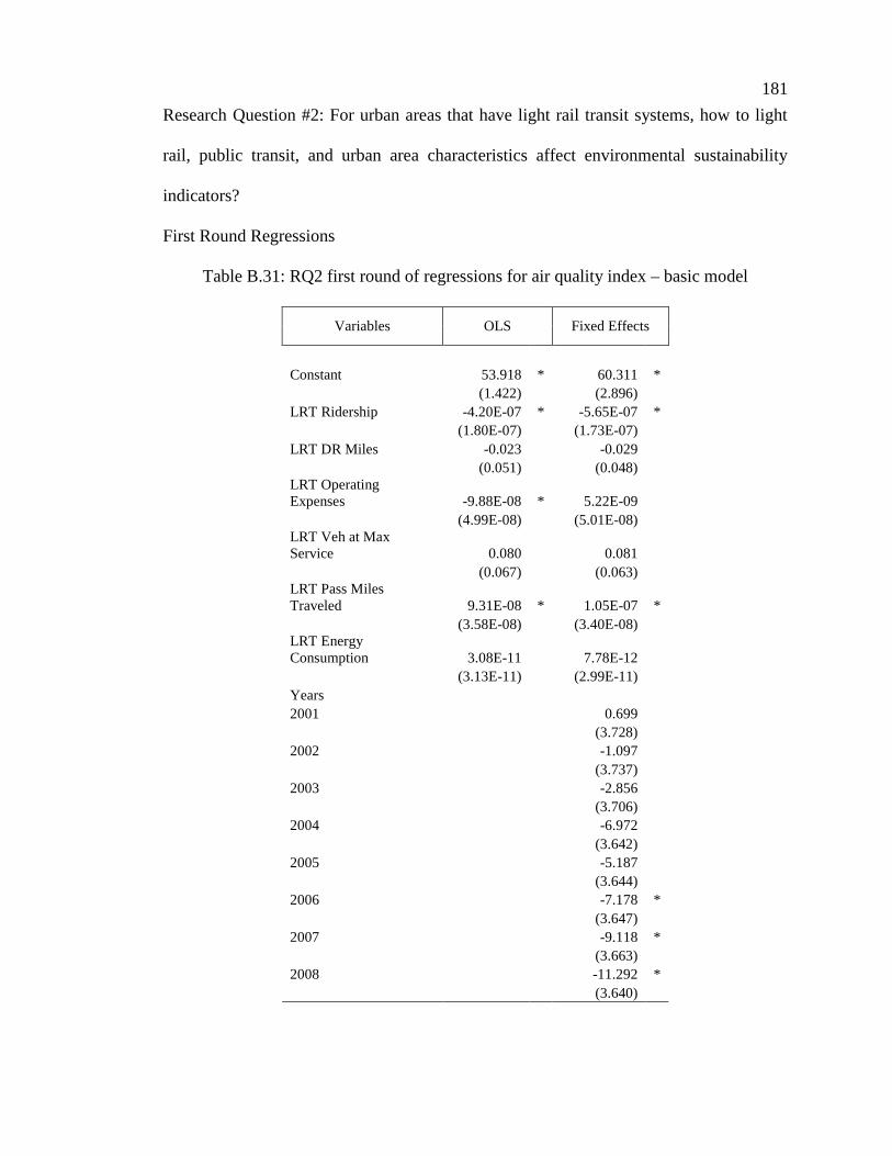
181
Research Question #2: For urban areas that have light rail transit systems, how to light
rail, public transit, and urban area characteristics affect environmental sustainability
indicators?
First Round Regressions
Table B.31: RQ2 first round of regressions for air quality index – basic model
Variables OLS Fixed Effects
Constant 53.918 * 60.311 *(1.422) (2.896)
LRT Ridership -4.20E-07 * -5.65E-07 *(1.80E-07) (1.73E-07)
LRT DR Miles -0.023 -0.029(0.051) (0.048)
LRT OperatingExpenses -9.88E-08 * 5.22E-09
(4.99E-08) (5.01E-08)LRT Veh at MaxService 0.080 0.081
(0.067) (0.063)LRT Pass MilesTraveled 9.31E-08 * 1.05E-07 *
(3.58E-08) (3.40E-08)LRT EnergyConsumption 3.08E-11 7.78E-12
(3.13E-11) (2.99E-11)Years2001 0.699
(3.728)2002 -1.097
(3.737)2003 -2.856
(3.706)2004 -6.972
(3.642)2005 -5.187
(3.644)2006 -7.178 *
(3.647)2007 -9.118 *
(3.663)2008 -11.292 *
(3.640)
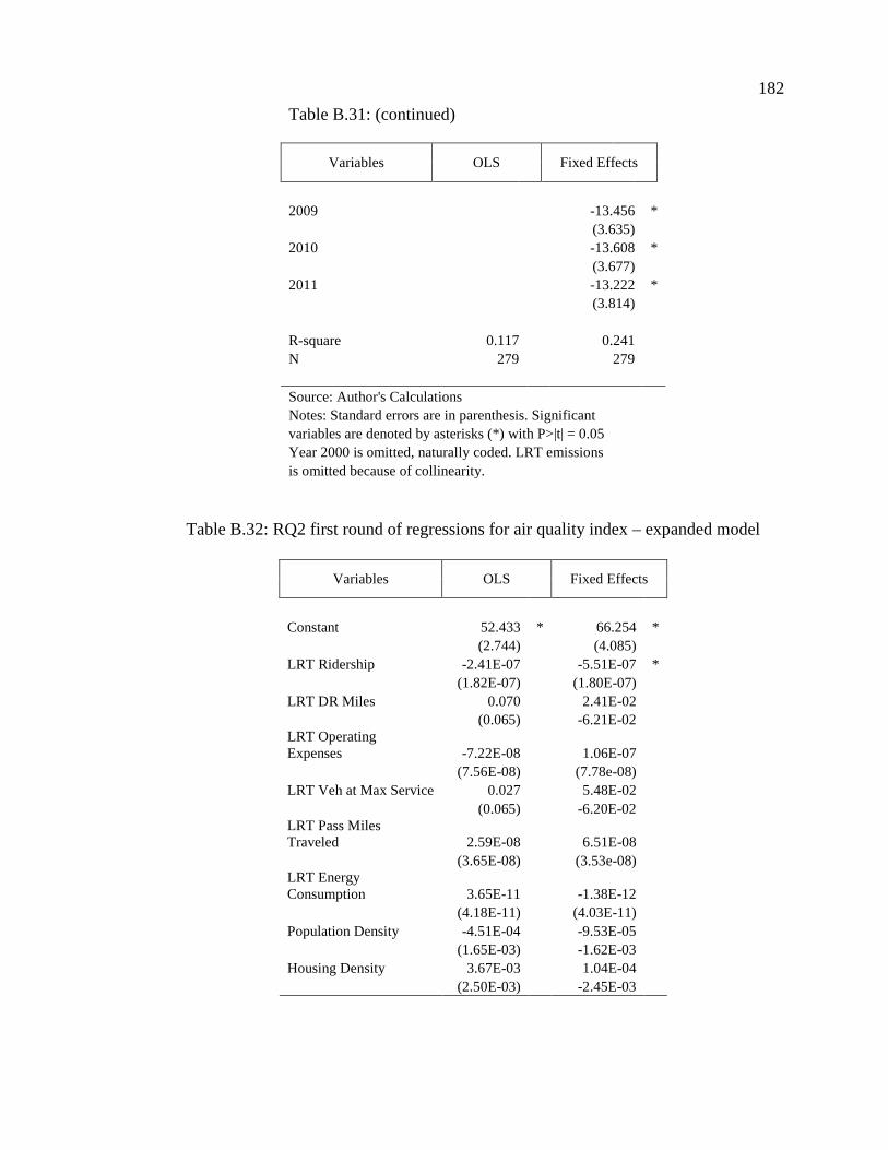
182
Table B.31: (continued)
Variables OLS Fixed Effects
2009 -13.456 *(3.635)
2010 -13.608 *(3.677)
2011 -13.222 *(3.814)
R-square 0.117 0.241N 279 279
Source: Author's CalculationsNotes: Standard errors are in parenthesis. Significantvariables are denoted by asterisks (*) with P>|t| = 0.05Year 2000 is omitted, naturally coded. LRT emissionsis omitted because of collinearity.
Table B.32: RQ2 first round of regressions for air quality index – expanded model
Variables OLS Fixed Effects
Constant 52.433 * 66.254 *(2.744) (4.085)
LRT Ridership -2.41E-07 -5.51E-07 *(1.82E-07) (1.80E-07)
LRT DR Miles 0.070 2.41E-02(0.065) -6.21E-02
LRT OperatingExpenses -7.22E-08 1.06E-07
(7.56E-08) (7.78e-08)LRT Veh at Max Service 0.027 5.48E-02
(0.065) -6.20E-02LRT Pass MilesTraveled 2.59E-08 6.51E-08
(3.65E-08) (3.53e-08)LRT EnergyConsumption 3.65E-11 -1.38E-12
(4.18E-11) (4.03E-11)Population Density -4.51E-04 -9.53E-05
(1.65E-03) -1.62E-03Housing Density 3.67E-03 1.04E-04
(2.50E-03) -2.45E-03
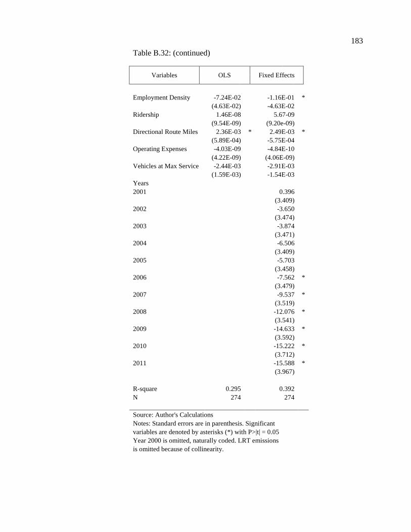
183
Table B.32: (continued)
Variables OLS Fixed Effects
Employment Density -7.24E-02 -1.16E-01 *(4.63E-02) -4.63E-02
Ridership 1.46E-08 5.67-09(9.54E-09) (9.20e-09)
Directional Route Miles 2.36E-03 * 2.49E-03 *(5.89E-04) -5.75E-04
Operating Expenses -4.03E-09 -4.84E-10(4.22E-09) (4.06E-09)
Vehicles at Max Service -2.44E-03 -2.91E-03(1.59E-03) -1.54E-03
Years2001 0.396
(3.409)2002 -3.650
(3.474)2003 -3.874
(3.471)2004 -6.506
(3.409)2005 -5.703
(3.458)2006 -7.562 *
(3.479)2007 -9.537 *
(3.519)2008 -12.076 *
(3.541)2009 -14.633 *
(3.592)2010 -15.222 *
(3.712)2011 -15.588 *
(3.967)
R-square 0.295 0.392N 274 274
Source: Author's CalculationsNotes: Standard errors are in parenthesis. Significantvariables are denoted by asterisks (*) with P>|t| = 0.05Year 2000 is omitted, naturally coded. LRT emissionsis omitted because of collinearity.
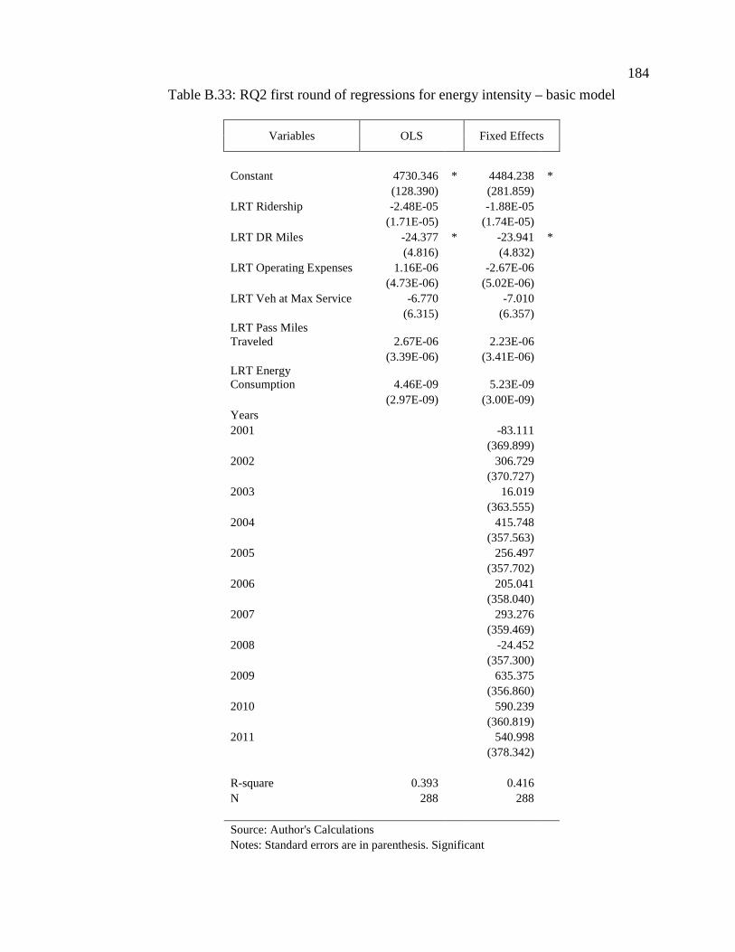
184
Table B.33: RQ2 first round of regressions for energy intensity – basic model
Variables OLS Fixed Effects
Constant 4730.346 * 4484.238 *(128.390) (281.859)
LRT Ridership -2.48E-05 -1.88E-05(1.71E-05) (1.74E-05)
LRT DR Miles -24.377 * -23.941 *(4.816) (4.832)
LRT Operating Expenses 1.16E-06 -2.67E-06(4.73E-06) (5.02E-06)
LRT Veh at Max Service -6.770 -7.010(6.315) (6.357)
LRT Pass MilesTraveled 2.67E-06 2.23E-06
(3.39E-06) (3.41E-06)LRT EnergyConsumption 4.46E-09 5.23E-09
(2.97E-09) (3.00E-09)Years2001 -83.111
(369.899)2002 306.729
(370.727)2003 16.019
(363.555)2004 415.748
(357.563)2005 256.497
(357.702)2006 205.041
(358.040)2007 293.276
(359.469)2008 -24.452
(357.300)2009 635.375
(356.860)2010 590.239
(360.819)2011 540.998
(378.342)
R-square 0.393 0.416N 288 288
Source: Author's CalculationsNotes: Standard errors are in parenthesis. Significant
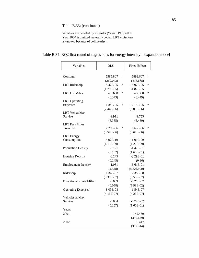
185
Table B.33: (continued)
variables are denoted by asterisks (*) with P>|t| = 0.05Year 2000 is omitted, naturally coded. LRT emissionsis omitted because of collinearity.
Table B.34: RQ2 first round of regressions for energy intensity – expanded model
Variables OLS Fixed Effects
Constant 5585.807 * 5892.607 *(269.043) (415.668)
LRT Ridership -5.47E-05 * -5.97E-05 *(1.79E-05) -1.87E-05
LRT DR Miles -26.638 * -27.390 *(6.343) (6.449)
LRT OperatingExpenses 1.84E-05 * -2.15E-05 *
(7.44E-06) (8.09E-06)LRT Veh at MaxService -2.911 -2.755
(6.385) (6.460)LRT Pass MilesTraveled 7.29E-06 * 8.63E-06 *
(3.59E-06) (3.67E-06)LRT EnergyConsumption -4.92E-10 -1.01E-09
(4.11E-09) (4.20E-09)Population Density -0.121 -1.47E-01
(0.162) (1.68E-01)Housing Density -0.245 -3.29E-01
(0.245) (0.26)Employment Density -1.081 -6.61E-01
(4.548) (4.82E+00)Ridership 1.34E-07 2.38E-08
(9.39E-07) (9.58E-07)Directional Route Miles -0.089 -8.28E-02
(0.058) (5.98E-02)Operating Expenses 8.03E-08 1.54E-07
(4.15E-07) (4.23E-07)Vehicles at MaxService -0.064 -8.74E-02
(0.157) (1.60E-01)Years2001 -142.459
(350.479)2002 195.447
(357.314)
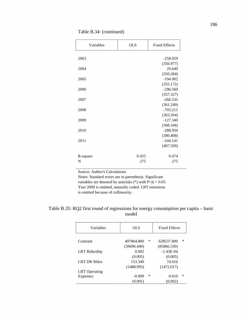
186
Table B.34: (continued)
Variables OLS Fixed Effects
2003 -258.059(356.977)
2004 29.640(350.284)
2005 -194.902(355.172)
2006 -296.560(357.327)
2007 -266.535(361.249)
2008 -703.211(363.204)
2009 -127.340(368.166)
2010 -288.950(380.408)
2011 -244.141(407.569)
R-square 0.455 0.474N 275 275
Source: Author's CalculationsNotes: Standard errors are in parenthesis. Significantvariables are denoted by asterisks (*) with P>|t| = 0.05Year 2000 is omitted, naturally coded. LRT emissionsis omitted because of collinearity.
Table B.35: RQ2 first round of regressions for energy consumption per capita – basicmodel
Variables OLS Fixed Effects
Constant 497864.800 * 628537.800 *(39696.440) (85866.530)
LRT Ridership 0.002 -1.43E-04(0.005) (0.005)
LRT DR Miles 153.349 74.016(1488.993) (1472.017)
LRT OperatingExpenses -0.009 * 0.010 *
(0.001) (0.002)
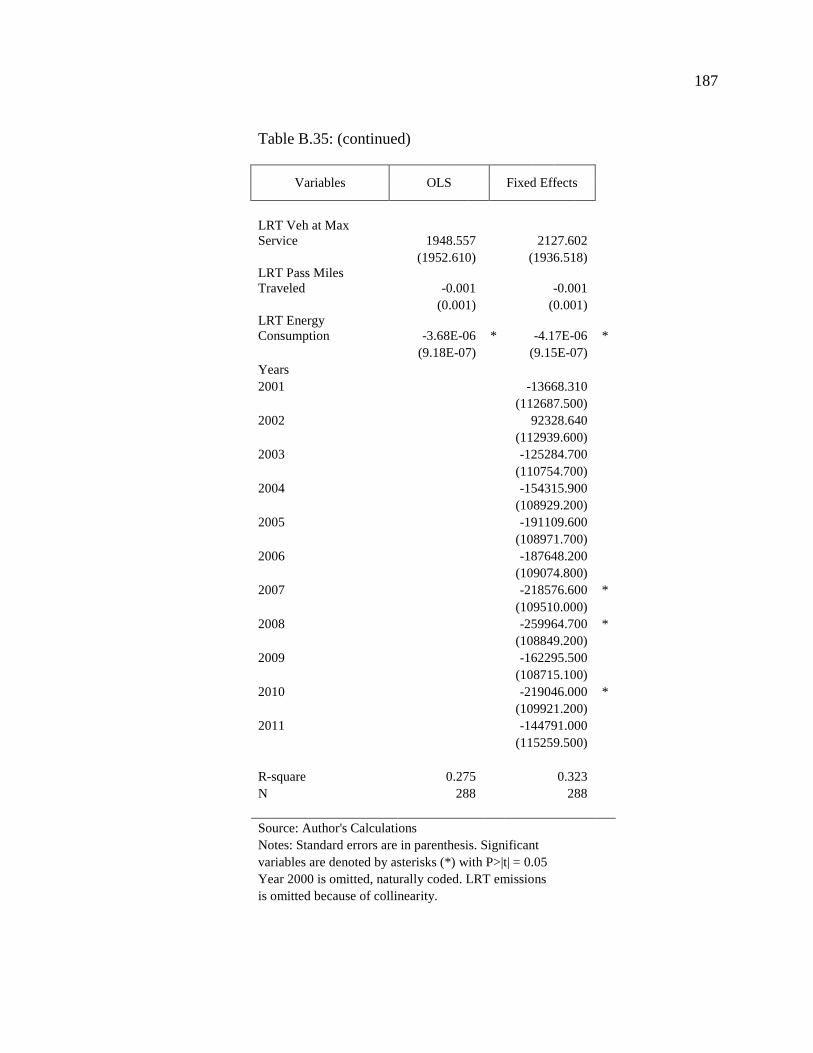
187
Table B.35: (continued)
Variables OLS Fixed Effects
LRT Veh at MaxService 1948.557 2127.602
(1952.610) (1936.518)LRT Pass MilesTraveled -0.001 -0.001
(0.001) (0.001)LRT EnergyConsumption -3.68E-06 * -4.17E-06 *
(9.18E-07) (9.15E-07)Years2001 -13668.310
(112687.500)2002 92328.640
(112939.600)2003 -125284.700
(110754.700)2004 -154315.900
(108929.200)2005 -191109.600
(108971.700)2006 -187648.200
(109074.800)2007 -218576.600 *
(109510.000)2008 -259964.700 *
(108849.200)2009 -162295.500
(108715.100)2010 -219046.000 *
(109921.200)2011 -144791.000
(115259.500)
R-square 0.275 0.323N 288 288
Source: Author's CalculationsNotes: Standard errors are in parenthesis. Significantvariables are denoted by asterisks (*) with P>|t| = 0.05Year 2000 is omitted, naturally coded. LRT emissionsis omitted because of collinearity.
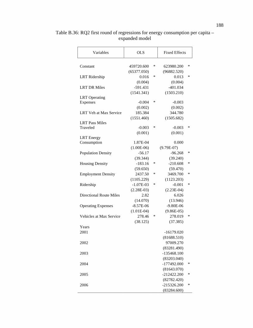
188
Table B.36: RQ2 first round of regressions for energy consumption per capita –expanded model
Variables OLS Fixed Effects
Constant 459720.600 * 623980.200 *(65377.050) (96882.520)
LRT Ridership 0.016 * 0.013 *(0.004) (0.004)
LRT DR Miles -591.431 -401.034(1541.341) (1503.210)
LRT OperatingExpenses -0.004 * -0.003
(0.002) (0.002)LRT Veh at Max Service 185.384 344.780
(1551.460) (1505.682)LRT Pass MilesTraveled -0.003 * -0.003 *
(0.001) (0.001)LRT EnergyConsumption 1.87E-04 0.000
(1.00E-06) (9.79E-07)Population Density -56.17 -96.268 *
(39.344) (39.240)Housing Density -183.16 * -210.608 *
(59.650) (59.470)Employment Density 2437.50 * 3469.700 *
(1105.229) (1123.203)Ridership -1.07E-03 * -0.001 *
(2.28E-03) (2.23E-04)Directional Route Miles 2.82 6.026
(14.070) (13.946)Operating Expenses -8.57E-06 -9.80E-06
(1.01E-04) (9.86E-05)Vehicles at Max Service 278.46 * 278.019 *
(38.125) (37.385)Years2001 -16179.020
(81688.510)2002 97009.270
(83281.490)2003 -135468.100
(83203.040)2004 -177492.000 *
(81643.070)2005 -212422.200 *
(82782.420)2006 -215326.200 *
(83284.600)
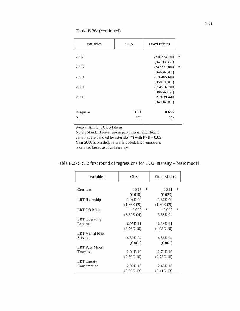
189
Table B.36: (continued)
Variables OLS Fixed Effects
2007 -210274.700 *(84198.830)
2008 -243777.800 *(84654.310)
2009 -130465.600(85810.810)
2010 -154516.700(88664.160)
2011 -93639.440(94994.910)
R-square 0.611 0.655N 275 275
Source: Author's CalculationsNotes: Standard errors are in parenthesis. Significantvariables are denoted by asterisks (*) with P>|t| = 0.05Year 2000 is omitted, naturally coded. LRT emissionsis omitted because of collinearity.
Table B.37: RQ2 first round of regressions for CO2 intensity – basic model
Variables OLS Fixed Effects
Constant 0.325 * 0.311 *(0.010) (0.023)
LRT Ridership -1.94E-09 -1.67E-09(1.36E-09) (1.39E-09)
LRT DR Miles -0.002 * -0.002 *(3.82E-04) -3.88E-04
LRT OperatingExpenses 6.95E-11 -6.84E-11
(3.76E-10) (4.03E-10)LRT Veh at MaxService -4.50E-04 -4.86E-04
(0.001) (0.001)LRT Pass MilesTraveled 2.91E-10 2.71E-10
(2.69E-10) (2.73E-10)LRT EnergyConsumption 2.09E-13 2.43E-13
(2.36E-13) (2.41E-13)
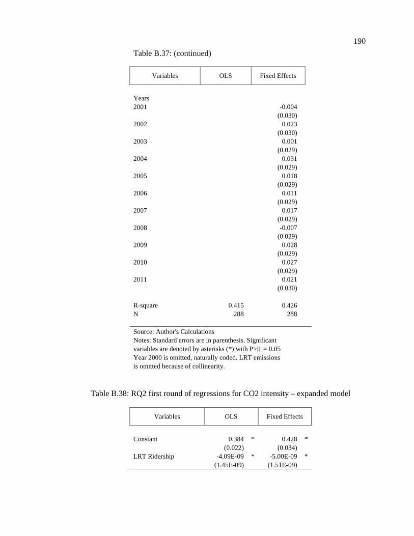
190
Table B.37: (continued)
Variables OLS Fixed Effects
Years2001 -0.004
(0.030)2002 0.023
(0.030)2003 0.001
(0.029)2004 0.031
(0.029)2005 0.018
(0.029)2006 0.011
(0.029)2007 0.017
(0.029)2008 -0.007
(0.029)2009 0.028
(0.029)2010 0.027
(0.029)2011 0.021
(0.030)
R-square 0.415 0.426N 288 288
Source: Author's CalculationsNotes: Standard errors are in parenthesis. Significantvariables are denoted by asterisks (*) with P>|t| = 0.05Year 2000 is omitted, naturally coded. LRT emissionsis omitted because of collinearity.
Table B.38: RQ2 first round of regressions for CO2 intensity – expanded model
Variables OLS Fixed Effects
Constant 0.384 * 0.428 *(0.022) (0.034)
LRT Ridership -4.09E-09 * -5.00E-09 *(1.45E-09) (1.51E-09)
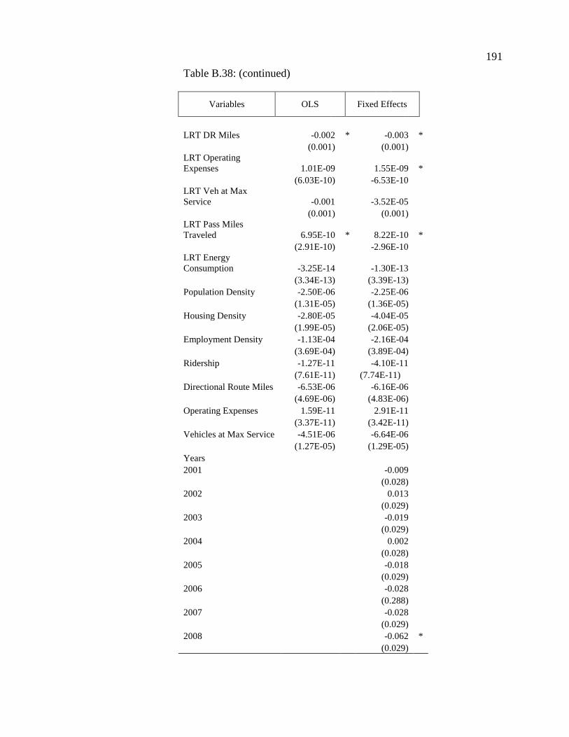
191
Table B.38: (continued)
Variables OLS Fixed Effects
LRT DR Miles -0.002 * -0.003 *(0.001) (0.001)
LRT OperatingExpenses 1.01E-09 1.55E-09 *
(6.03E-10) -6.53E-10LRT Veh at MaxService -0.001 -3.52E-05
(0.001) (0.001)LRT Pass MilesTraveled 6.95E-10 * 8.22E-10 *
(2.91E-10) -2.96E-10LRT EnergyConsumption -3.25E-14 -1.30E-13
(3.34E-13) (3.39E-13)Population Density -2.50E-06 -2.25E-06
(1.31E-05) (1.36E-05)Housing Density -2.80E-05 -4.04E-05
(1.99E-05) (2.06E-05)Employment Density -1.13E-04 -2.16E-04
(3.69E-04) (3.89E-04)Ridership -1.27E-11 -4.10E-11
(7.61E-11) (7.74E-11)Directional Route Miles -6.53E-06 -6.16E-06
(4.69E-06) (4.83E-06)Operating Expenses 1.59E-11 2.91E-11
(3.37E-11) (3.42E-11)Vehicles at Max Service -4.51E-06 -6.64E-06
(1.27E-05) (1.29E-05)Years2001 -0.009
(0.028)2002 0.013
(0.029)2003 -0.019
(0.029)2004 0.002
(0.028)2005 -0.018
(0.029)2006 -0.028
(0.288)2007 -0.028
(0.029)2008 -0.062 *
(0.029)
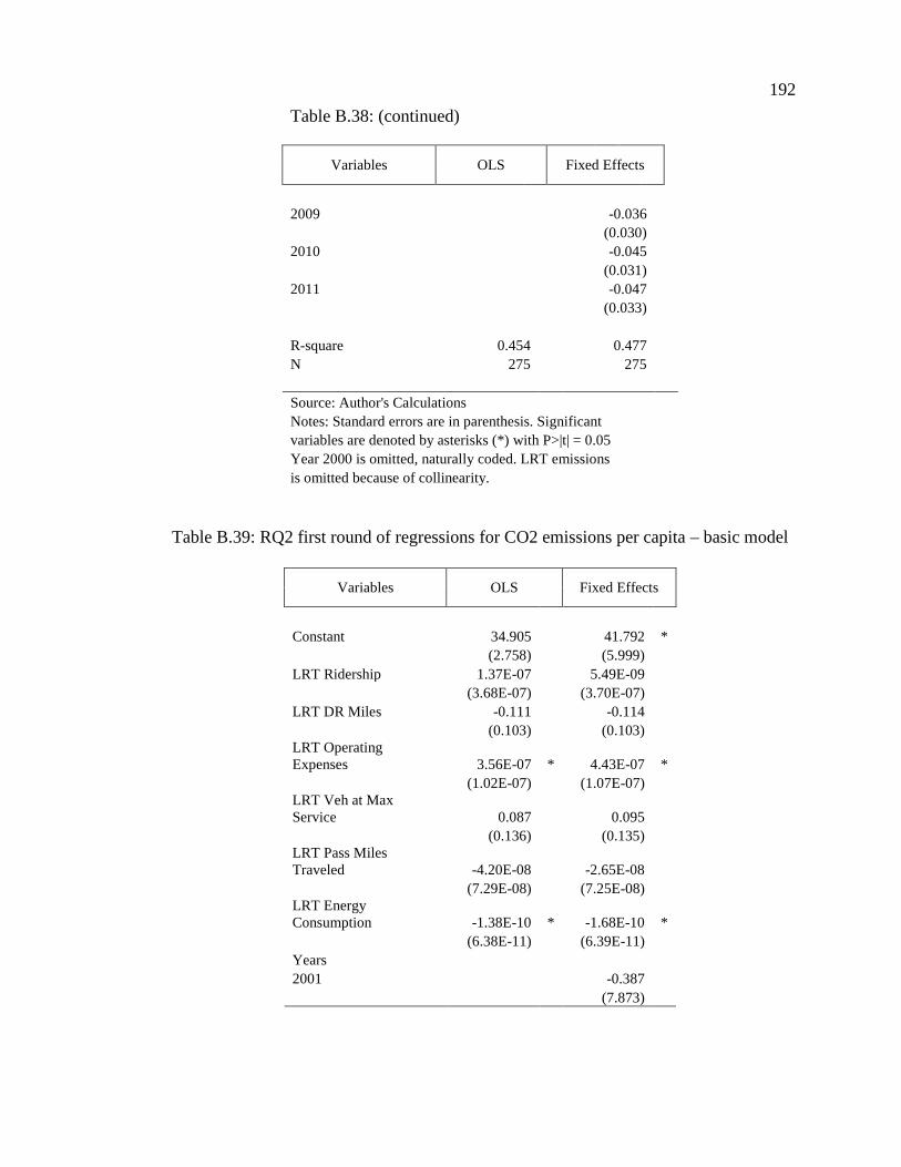
192
Table B.38: (continued)
Variables OLS Fixed Effects
2009 -0.036(0.030)
2010 -0.045(0.031)
2011 -0.047(0.033)
R-square 0.454 0.477N 275 275
Source: Author's CalculationsNotes: Standard errors are in parenthesis. Significantvariables are denoted by asterisks (*) with P>|t| = 0.05Year 2000 is omitted, naturally coded. LRT emissionsis omitted because of collinearity.
Table B.39: RQ2 first round of regressions for CO2 emissions per capita – basic model
Variables OLS Fixed Effects
Constant 34.905 41.792 *(2.758) (5.999)
LRT Ridership 1.37E-07 5.49E-09(3.68E-07) (3.70E-07)
LRT DR Miles -0.111 -0.114(0.103) (0.103)
LRT OperatingExpenses 3.56E-07 * 4.43E-07 *
(1.02E-07) (1.07E-07)LRT Veh at MaxService 0.087 0.095
(0.136) (0.135)LRT Pass MilesTraveled -4.20E-08 -2.65E-08
(7.29E-08) (7.25E-08)LRT EnergyConsumption -1.38E-10 * -1.68E-10 *
(6.38E-11) (6.39E-11)Years2001 -0.387
(7.873)
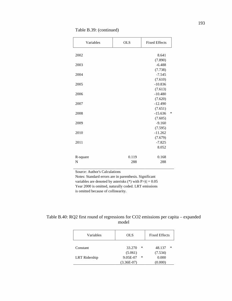
193
Table B.39: (continued)
Variables OLS Fixed Effects
2002 8.641(7.890)
2003 -6.488(7.738)
2004 -7.545(7.610)
2005 -10.836(7.613)
2006 -10.480(7.620)
2007 -12.490(7.651)
2008 -15.636 *(7.605)
2009 -9.160(7.595)
2010 -11.262(7.679)
2011 -7.8258.052
R-square 0.119 0.168N 288 288
Source: Author's CalculationsNotes: Standard errors are in parenthesis. Significantvariables are denoted by asterisks (*) with P>|t| = 0.05Year 2000 is omitted, naturally coded. LRT emissionsis omitted because of collinearity.
Table B.40: RQ2 first round of regressions for CO2 emissions per capita – expandedmodel
Variables OLS Fixed Effects
Constant 33.270 * 48.137 *(5.061) (7.534)
LRT Ridership 9.05E-07 * 0.000(3.36E-07) (0.000)
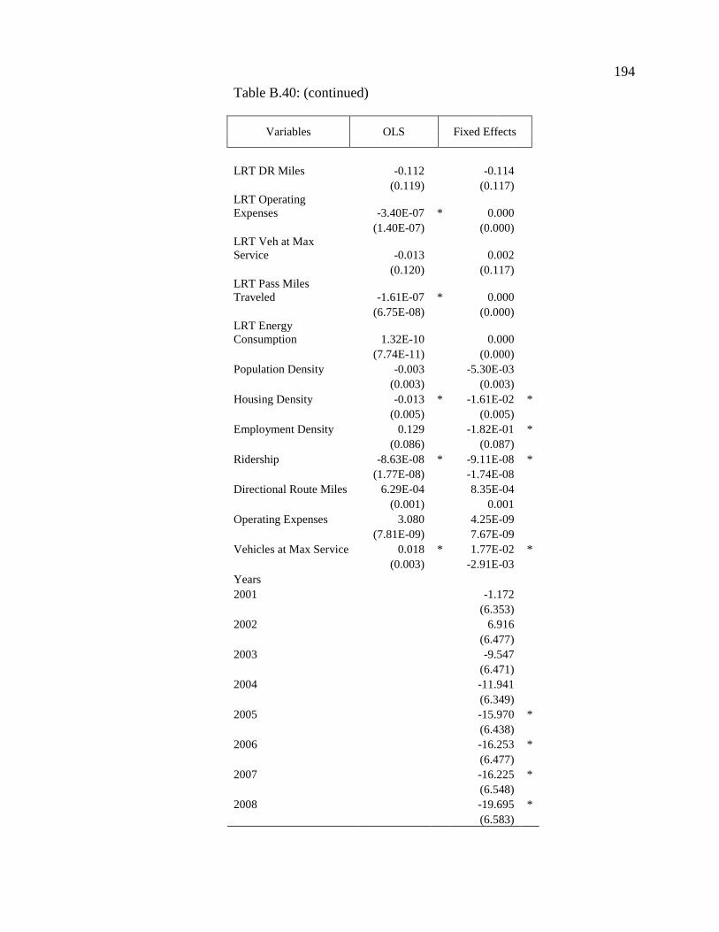
194
Table B.40: (continued)
Variables OLS Fixed Effects
LRT DR Miles -0.112 -0.114(0.119) (0.117)
LRT OperatingExpenses -3.40E-07 * 0.000
(1.40E-07) (0.000)LRT Veh at MaxService -0.013 0.002
(0.120) (0.117)LRT Pass MilesTraveled -1.61E-07 * 0.000
(6.75E-08) (0.000)LRT EnergyConsumption 1.32E-10 0.000
(7.74E-11) (0.000)Population Density -0.003 -5.30E-03
(0.003) (0.003)Housing Density -0.013 * -1.61E-02 *
(0.005) (0.005)Employment Density 0.129 -1.82E-01 *
(0.086) (0.087)Ridership -8.63E-08 * -9.11E-08 *
(1.77E-08) -1.74E-08Directional Route Miles 6.29E-04 8.35E-04
(0.001) 0.001Operating Expenses 3.080 4.25E-09
(7.81E-09) 7.67E-09Vehicles at Max Service 0.018 * 1.77E-02 *
(0.003) -2.91E-03Years2001 -1.172
(6.353)2002 6.916
(6.477)2003 -9.547
(6.471)2004 -11.941
(6.349)2005 -15.970 *
(6.438)2006 -16.253 *
(6.477)2007 -16.225 *
(6.548)2008 -19.695 *
(6.583)
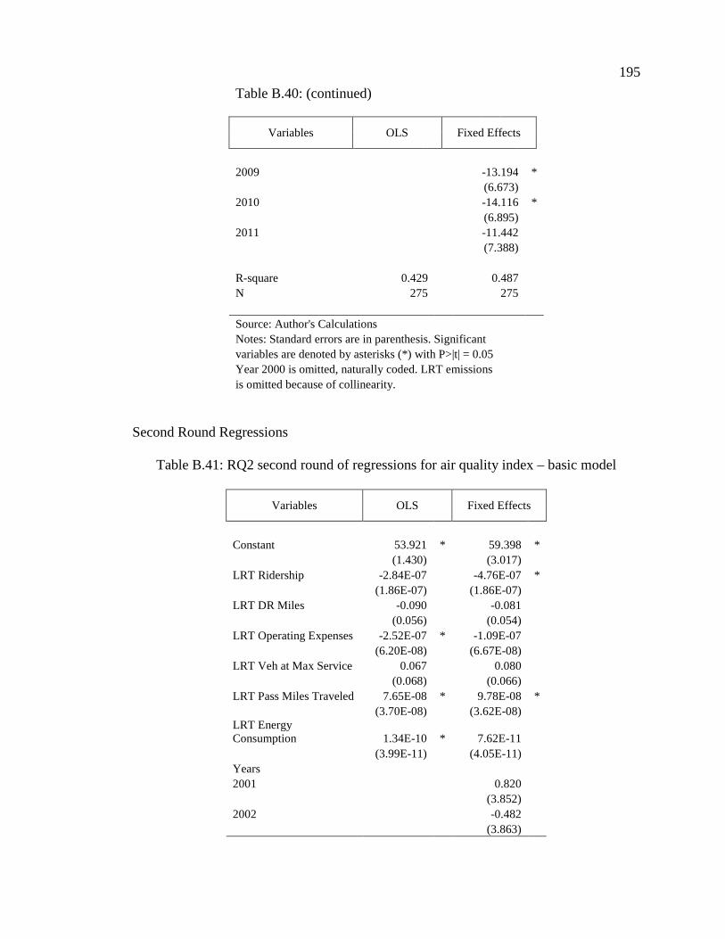
195
Table B.40: (continued)
Variables OLS Fixed Effects
2009 -13.194 *(6.673)
2010 -14.116 *(6.895)
2011 -11.442(7.388)
R-square 0.429 0.487N 275 275
Source: Author's CalculationsNotes: Standard errors are in parenthesis. Significantvariables are denoted by asterisks (*) with P>|t| = 0.05Year 2000 is omitted, naturally coded. LRT emissionsis omitted because of collinearity.
Second Round Regressions
Table B.41: RQ2 second round of regressions for air quality index – basic model
Variables OLS Fixed Effects
Constant 53.921 * 59.398 *(1.430) (3.017)
LRT Ridership -2.84E-07 -4.76E-07 *(1.86E-07) (1.86E-07)
LRT DR Miles -0.090 -0.081(0.056) (0.054)
LRT Operating Expenses -2.52E-07 * -1.09E-07(6.20E-08) (6.67E-08)
LRT Veh at Max Service 0.067 0.080(0.068) (0.066)
LRT Pass Miles Traveled 7.65E-08 * 9.78E-08 *(3.70E-08) (3.62E-08)
LRT EnergyConsumption 1.34E-10 * 7.62E-11
(3.99E-11) (4.05E-11)Years2001 0.820
(3.852)2002 -0.482
(3.863)
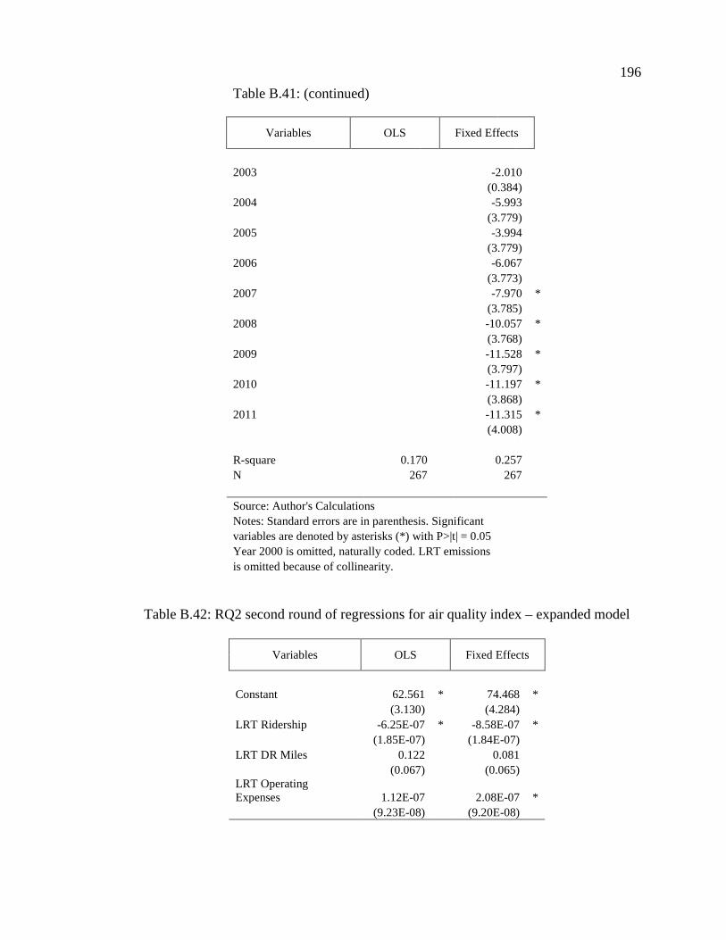
196
Table B.41: (continued)
Variables OLS Fixed Effects
2003 -2.010(0.384)
2004 -5.993(3.779)
2005 -3.994(3.779)
2006 -6.067(3.773)
2007 -7.970 *(3.785)
2008 -10.057 *(3.768)
2009 -11.528 *(3.797)
2010 -11.197 *(3.868)
2011 -11.315 *(4.008)
R-square 0.170 0.257N 267 267
Source: Author's CalculationsNotes: Standard errors are in parenthesis. Significantvariables are denoted by asterisks (*) with P>|t| = 0.05Year 2000 is omitted, naturally coded. LRT emissionsis omitted because of collinearity.
Table B.42: RQ2 second round of regressions for air quality index – expanded model
Variables OLS Fixed Effects
Constant 62.561 * 74.468 *(3.130) (4.284)
LRT Ridership -6.25E-07 * -8.58E-07 *(1.85E-07) (1.84E-07)
LRT DR Miles 0.122 0.081(0.067) (0.065)
LRT OperatingExpenses 1.12E-07 2.08E-07 *
(9.23E-08) (9.20E-08)
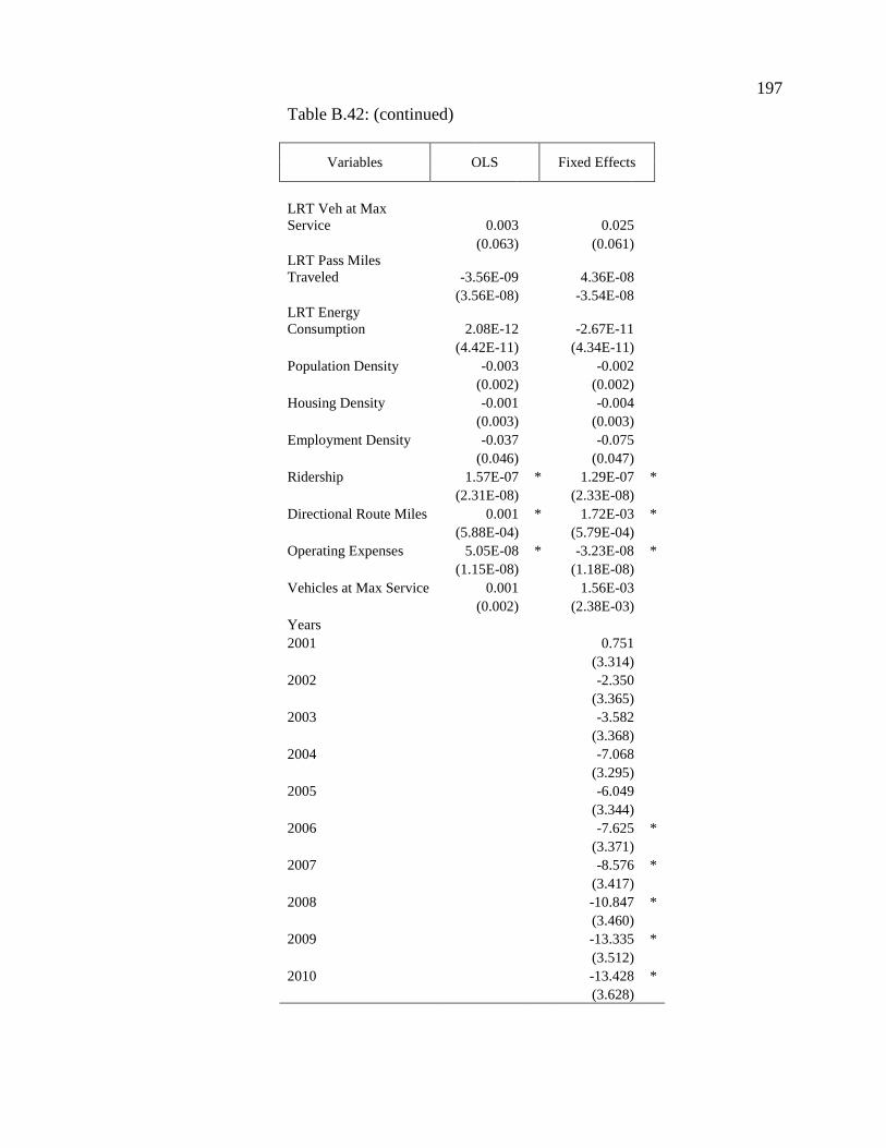
197
Table B.42: (continued)
Variables OLS Fixed Effects
LRT Veh at MaxService 0.003 0.025
(0.063) (0.061)LRT Pass MilesTraveled -3.56E-09 4.36E-08
(3.56E-08) -3.54E-08LRT EnergyConsumption 2.08E-12 -2.67E-11
(4.42E-11) (4.34E-11)Population Density -0.003 -0.002
(0.002) (0.002)Housing Density -0.001 -0.004
(0.003) (0.003)Employment Density -0.037 -0.075
(0.046) (0.047)Ridership 1.57E-07 * 1.29E-07 *
(2.31E-08) (2.33E-08)Directional Route Miles 0.001 * 1.72E-03 *
(5.88E-04) (5.79E-04)Operating Expenses 5.05E-08 * -3.23E-08 *
(1.15E-08) (1.18E-08)Vehicles at Max Service 0.001 1.56E-03
(0.002) (2.38E-03)Years2001 0.751
(3.314)2002 -2.350
(3.365)2003 -3.582
(3.368)2004 -7.068
(3.295)2005 -6.049
(3.344)2006 -7.625 *
(3.371)2007 -8.576 *
(3.417)2008 -10.847 *
(3.460)2009 -13.335 *
(3.512)2010 -13.428 *
(3.628)
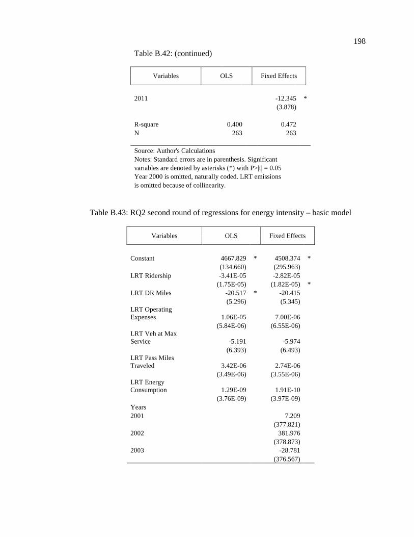
198
Table B.42: (continued)
Variables OLS Fixed Effects
2011 -12.345 *(3.878)
R-square 0.400 0.472N 263 263
Source: Author's CalculationsNotes: Standard errors are in parenthesis. Significantvariables are denoted by asterisks (*) with P>|t| = 0.05Year 2000 is omitted, naturally coded. LRT emissionsis omitted because of collinearity.
Table B.43: RQ2 second round of regressions for energy intensity – basic model
Variables OLS Fixed Effects
Constant 4667.829 * 4508.374 *(134.660) (295.963)
LRT Ridership -3.41E-05 -2.82E-05(1.75E-05) (1.82E-05) *
LRT DR Miles -20.517 * -20.415(5.296) (5.345)
LRT OperatingExpenses 1.06E-05 7.00E-06
(5.84E-06) (6.55E-06)LRT Veh at MaxService -5.191 -5.974
(6.393) (6.493)LRT Pass MilesTraveled 3.42E-06 2.74E-06
(3.49E-06) (3.55E-06)LRT EnergyConsumption 1.29E-09 1.91E-10
(3.76E-09) (3.97E-09)Years2001 7.209
(377.821)2002 381.976
(378.873)2003 -28.781
(376.567)
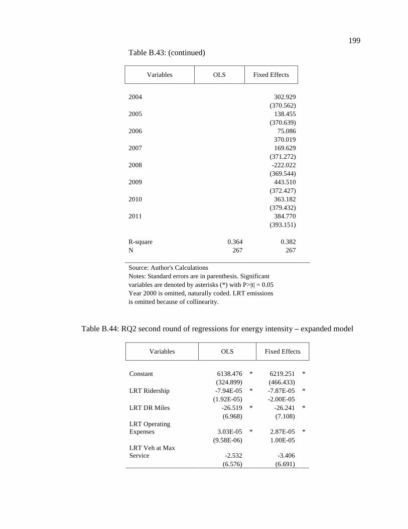
199
Table B.43: (continued)
Variables OLS Fixed Effects
2004 302.929(370.562)
2005 138.455(370.639)
2006 75.086370.019
2007 169.629(371.272)
2008 -222.022(369.544)
2009 443.510(372.427)
2010 363.182(379.432)
2011 384.770(393.151)
R-square 0.364 0.382N 267 267
Source: Author's CalculationsNotes: Standard errors are in parenthesis. Significantvariables are denoted by asterisks (*) with P>|t| = 0.05Year 2000 is omitted, naturally coded. LRT emissionsis omitted because of collinearity.
Table B.44: RQ2 second round of regressions for energy intensity – expanded model
Variables OLS Fixed Effects
Constant 6138.476 * 6219.251 *(324.899) (466.433)
LRT Ridership -7.94E-05 * -7.87E-05 *(1.92E-05) -2.00E-05
LRT DR Miles -26.519 * -26.241 *(6.968) (7.108)
LRT OperatingExpenses 3.03E-05 * 2.87E-05 *
(9.58E-06) 1.00E-05LRT Veh at MaxService -2.532 -3.406
(6.576) (6.691)
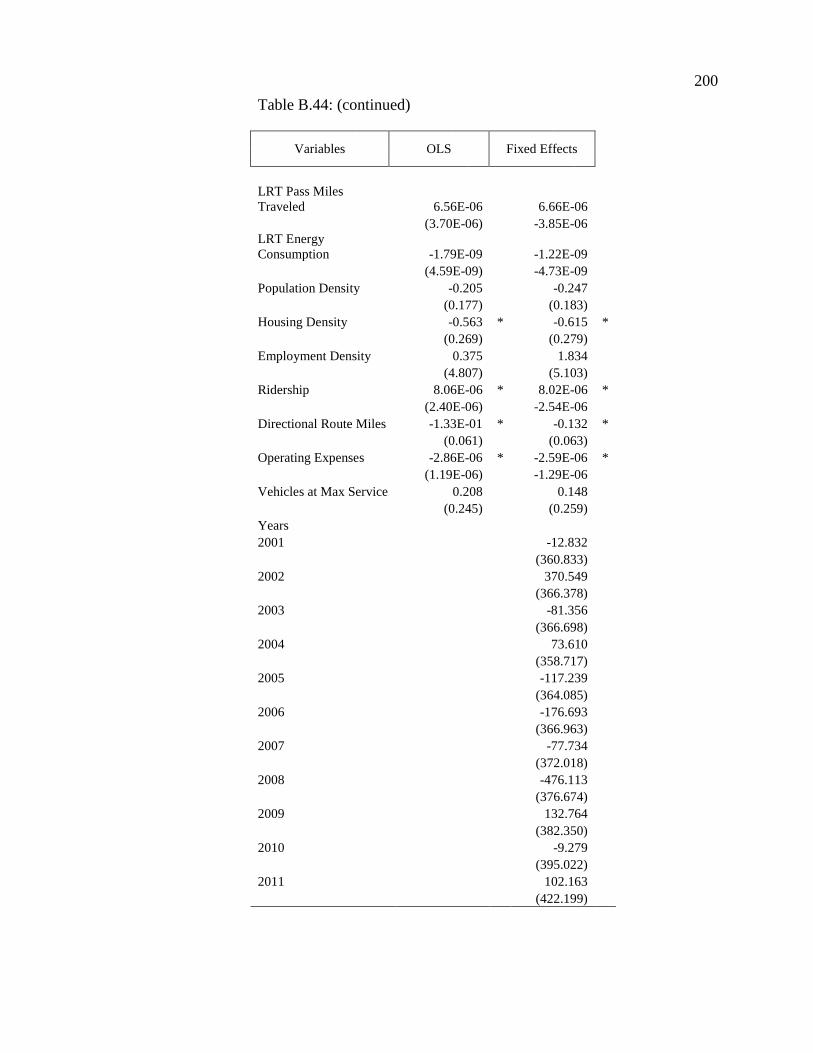
200
Table B.44: (continued)
Variables OLS Fixed Effects
LRT Pass MilesTraveled 6.56E-06 6.66E-06
(3.70E-06) -3.85E-06LRT EnergyConsumption -1.79E-09 -1.22E-09
(4.59E-09) -4.73E-09Population Density -0.205 -0.247
(0.177) (0.183)Housing Density -0.563 * -0.615 *
(0.269) (0.279)Employment Density 0.375 1.834
(4.807) (5.103)Ridership 8.06E-06 * 8.02E-06 *
(2.40E-06) -2.54E-06Directional Route Miles -1.33E-01 * -0.132 *
(0.061) (0.063)Operating Expenses -2.86E-06 * -2.59E-06 *
(1.19E-06) -1.29E-06Vehicles at Max Service 0.208 0.148
(0.245) (0.259)Years2001 -12.832
(360.833)2002 370.549
(366.378)2003 -81.356
(366.698)2004 73.610
(358.717)2005 -117.239
(364.085)2006 -176.693
(366.963)2007 -77.734
(372.018)2008 -476.113
(376.674)2009 132.764
(382.350)2010 -9.279
(395.022)2011 102.163
(422.199)
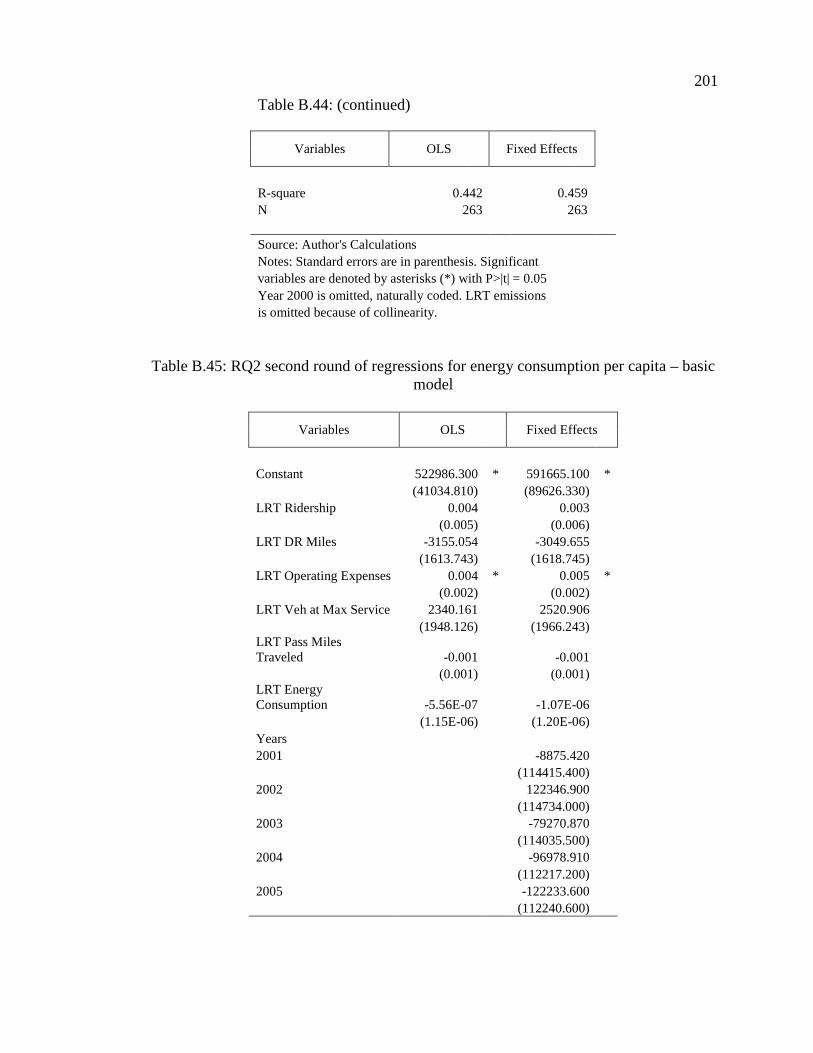
201
Table B.44: (continued)
Variables OLS Fixed Effects
R-square 0.442 0.459N 263 263
Source: Author's CalculationsNotes: Standard errors are in parenthesis. Significantvariables are denoted by asterisks (*) with P>|t| = 0.05Year 2000 is omitted, naturally coded. LRT emissionsis omitted because of collinearity.
Table B.45: RQ2 second round of regressions for energy consumption per capita – basicmodel
Variables OLS Fixed Effects
Constant 522986.300 * 591665.100 *(41034.810) (89626.330)
LRT Ridership 0.004 0.003(0.005) (0.006)
LRT DR Miles -3155.054 -3049.655(1613.743) (1618.745)
LRT Operating Expenses 0.004 * 0.005 *(0.002) (0.002)
LRT Veh at Max Service 2340.161 2520.906(1948.126) (1966.243)
LRT Pass MilesTraveled -0.001 -0.001
(0.001) (0.001)LRT EnergyConsumption -5.56E-07 -1.07E-06
(1.15E-06) (1.20E-06)Years2001 -8875.420
(114415.400)2002 122346.900
(114734.000)2003 -79270.870
(114035.500)2004 -96978.910
(112217.200)2005 -122233.600
(112240.600)
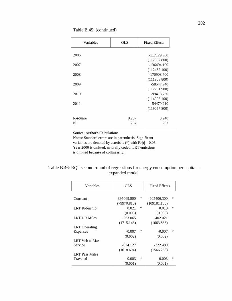
202
Table B.45: (continued)
Variables OLS Fixed Effects
2006 -117129.900(112052.800)
2007 -136494.100(112432.100)
2008 -170908.700(111908.800)
2009 -58547.940(112781.900)
2010 -99418.760(114903.100)
2011 -54470.210(119057.800)
R-square 0.207 0.240N 267 267
Source: Author's CalculationsNotes: Standard errors are in parenthesis. Significantvariables are denoted by asterisks (*) with P>|t| = 0.05Year 2000 is omitted, naturally coded. LRT emissionsis omitted because of collinearity.
Table B.46: RQ2 second round of regressions for energy consumption per capita –expanded model
Variables OLS Fixed Effects
Constant 395069.800 * 605406.300 *(79970.810) (109181.100)
LRT Ridership 0.021 * 0.018 *(0.005) (0.005)
LRT DR Miles -253.065 -402.021(1715.143) (1663.833)
LRT OperatingExpenses -0.007 * -0.007 *
(0.002) (0.002)LRT Veh at MaxService -674.127 -722.489
(1618.604) (1566.268)LRT Pass MilesTraveled -0.003 * -0.003 *
(0.001) (0.001)
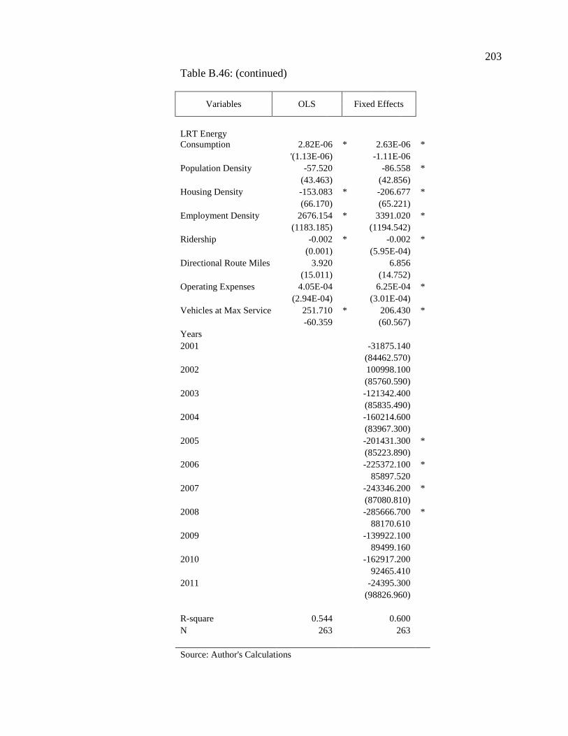
203
Table B.46: (continued)
Variables OLS Fixed Effects
LRT EnergyConsumption 2.82E-06 * 2.63E-06 *
'(1.13E-06) -1.11E-06Population Density -57.520 -86.558 *
(43.463) (42.856)Housing Density -153.083 * -206.677 *
(66.170) (65.221)Employment Density 2676.154 * 3391.020 *
(1183.185) (1194.542)Ridership -0.002 * -0.002 *
(0.001) (5.95E-04)Directional Route Miles 3.920 6.856
(15.011) (14.752)Operating Expenses 4.05E-04 6.25E-04 *
(2.94E-04) (3.01E-04)Vehicles at Max Service 251.710 * 206.430 *
-60.359 (60.567)Years2001 -31875.140
(84462.570)2002 100998.100
(85760.590)2003 -121342.400
(85835.490)2004 -160214.600
(83967.300)2005 -201431.300 *
(85223.890)2006 -225372.100 *
85897.5202007 -243346.200 *
(87080.810)2008 -285666.700 *
88170.6102009 -139922.100
89499.1602010 -162917.200
92465.4102011 -24395.300
(98826.960)
R-square 0.544 0.600N 263 263
Source: Author's Calculations
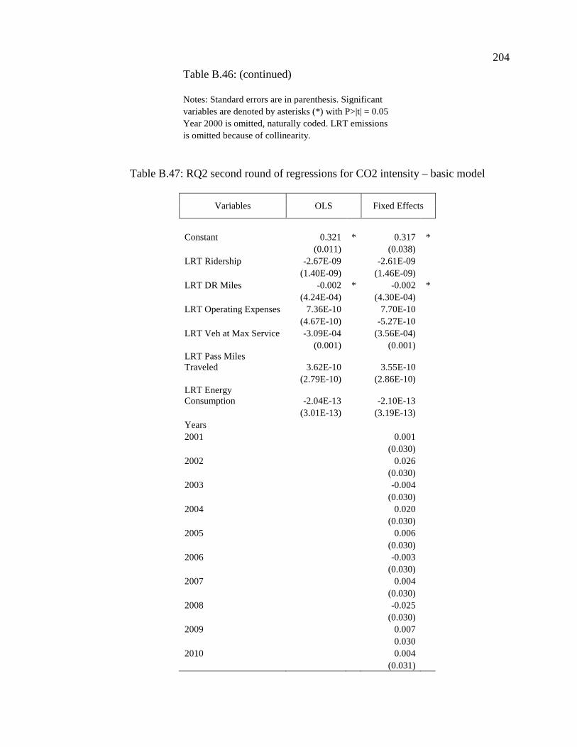
204
Table B.46: (continued)
Notes: Standard errors are in parenthesis. Significantvariables are denoted by asterisks (*) with P>|t| = 0.05Year 2000 is omitted, naturally coded. LRT emissionsis omitted because of collinearity.
Table B.47: RQ2 second round of regressions for CO2 intensity – basic model
Variables OLS Fixed Effects
Constant 0.321 * 0.317 *(0.011) (0.038)
LRT Ridership -2.67E-09 -2.61E-09(1.40E-09) (1.46E-09)
LRT DR Miles -0.002 * -0.002 *(4.24E-04) (4.30E-04)
LRT Operating Expenses 7.36E-10 7.70E-10(4.67E-10) -5.27E-10
LRT Veh at Max Service -3.09E-04 (3.56E-04)(0.001) (0.001)
LRT Pass MilesTraveled 3.62E-10 3.55E-10
(2.79E-10) (2.86E-10)LRT EnergyConsumption -2.04E-13 -2.10E-13
(3.01E-13) (3.19E-13)Years2001 0.001
(0.030)2002 0.026
(0.030)2003 -0.004
(0.030)2004 0.020
(0.030)2005 0.006
(0.030)2006 -0.003
(0.030)2007 0.004
(0.030)2008 -0.025
(0.030)2009 0.007
0.0302010 0.004
(0.031)
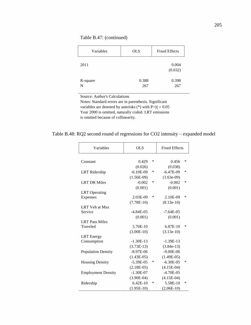
205
Table B.47: (continued)
Variables OLS Fixed Effects
2011 0.004(0.032)
R-square 0.388 0.398N 267 267
Source: Author's CalculationsNotes: Standard errors are in parenthesis. Significantvariables are denoted by asterisks (*) with P>|t| = 0.05Year 2000 is omitted, naturally coded. LRT emissionsis omitted because of collinearity.
Table B.48: RQ2 second round of regressions for CO2 intensity – expanded model
Variables OLS Fixed Effects
Constant 0.429 * 0.456 *(0.026) (0.038)
LRT Ridership -6.10E-09 * -6.47E-09 *(1.56E-09) (1.63e-09)
LRT DR Miles -0.002 * -0.002 *(0.001) (0.001)
LRT OperatingExpenses 2.03E-09 * 2.10E-09 *
(7.78E-10) (8.13e-10)LRT Veh at MaxService -4.84E-05 -7.64E-05
(0.001) (0.001)LRT Pass MilesTraveled 5.70E-10 6.87E-10 *
(3.00E-10) (3.13e-10)LRT EnergyConsumption -1.30E-13 -1.39E-13
(3.73E-13) (3.84e-13)Population Density -8.97E-06 -9.00E-06
(1.43E-05) (1.49E-05)Housing Density -5.39E-05 * -6.30E-05 *
(2.18E-05) (4.15E-04)Employment Density -1.30E-07 -4.70E-05
(3.90E-04) (4.15E-04)Ridership 6.42E-10 * 5.58E-10 *
(1.95E-10) (2.06E-10)
206
Table B.48: (continued)
Variables OLS Fixed Effects
Directional Route Miles -1.04E-05 * -9.93E-06(4.95E-06) (5.12e-06)
Operating Expenses -2.41E-10 * -1.75E-10(9.69E-11) (1.04e-10)
Vehicles at Max Service 2.14E-05 1.07E-05(1.99E-05) (2.10E-05)
Years2001 -0.002
(0.029)2002 0.024
(0.029)2003 -0.008
(0.030)2004 0.003
(0.029)2005 -0.014
(0.030)2006 -0.023
(0.030)2007 -0.017
(0.030)2008 -0.047
(0.031)2009 -0.019
(0.031)2010 -0.027
(0.032)2011 -0.023
(0.034)
R-square 0.448 0.464N 263 263
Source: Author's CalculationsNotes: Standard errors are in parenthesis. Significantvariables are denoted by asterisks (*) with P>|t| = 0.05Year 2000 is omitted, naturally coded. LRT emissionsis omitted because of collinearity.
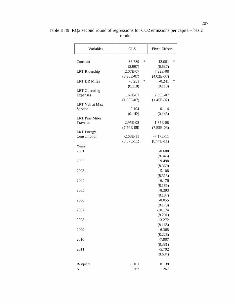
207
Table B.49: RQ2 second round of regressions for CO2 emissions per capita – basicmodel
Variables OLS Fixed Effects
Constant 36.789 * 42.081 *(2.997) (6.537)
LRT Ridership 2.07E-07 7.22E-08(3.90E-07) (4.02E-07)
LRT DR Miles -0.251 * -0.241 *(0.118) (0.118)
LRT OperatingExpenses 1.67E-07 2.69E-07
(1.30E-07) (1.45E-07)LRT Veh at MaxService 0.104 0.114
(0.142) (0.143)LRT Pass MilesTraveled -2.95E-08 -1.35E-08
(7.76E-08) (7.85E-08)LRT EnergyConsumption -2.68E-11 -7.17E-11
(8.37E-11) (8.77E-11)Years2001 -0.680
(8.346)2002 9.498
(8.369)2003 -5.108
(8.318)2004 -6.176
(8.185)2005 -8.293
(8.187)2006 -8.855
(8.173)2007 -10.174
(8.201)2008 -13.272
(8.163)2009 -6.365
(8.226)2010 -7.907
(8.381)2011 -5.792
(8.684)
R-square 0.101 0.139N 267 267
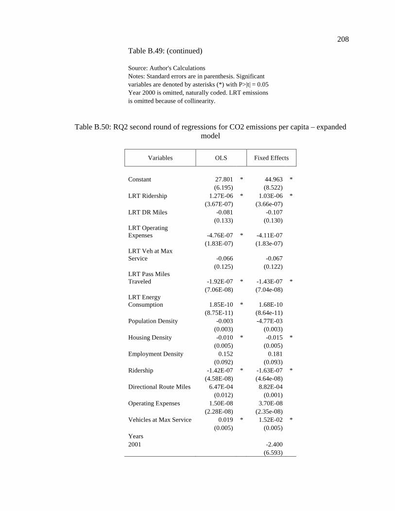
208
Table B.49: (continued)
Source: Author's CalculationsNotes: Standard errors are in parenthesis. Significantvariables are denoted by asterisks (*) with P>|t| = 0.05Year 2000 is omitted, naturally coded. LRT emissionsis omitted because of collinearity.
Table B.50: RQ2 second round of regressions for CO2 emissions per capita – expandedmodel
Variables OLS Fixed Effects
Constant 27.801 * 44.963 *(6.195) (8.522)
LRT Ridership 1.27E-06 * 1.03E-06 *(3.67E-07) (3.66e-07)
LRT DR Miles -0.081 -0.107(0.133) (0.130)
LRT OperatingExpenses -4.76E-07 * -4.11E-07
(1.83E-07) (1.83e-07)LRT Veh at MaxService -0.066 -0.067
(0.125) (0.122)LRT Pass MilesTraveled -1.92E-07 * -1.43E-07 *
(7.06E-08) (7.04e-08)LRT EnergyConsumption 1.85E-10 * 1.68E-10
(8.75E-11) (8.64e-11)Population Density -0.003 -4.77E-03
(0.003) (0.003)Housing Density -0.010 * -0.015 *
(0.005) (0.005)Employment Density 0.152 0.181
(0.092) (0.093)Ridership -1.42E-07 * -1.63E-07 *
(4.58E-08) (4.64e-08)Directional Route Miles 6.47E-04 8.82E-04
(0.012) (0.001)Operating Expenses 1.50E-08 3.70E-08
(2.28E-08) (2.35e-08)Vehicles at Max Service 0.019 * 1.52E-02 *
(0.005) (0.005)Years2001 -2.400
(6.593)
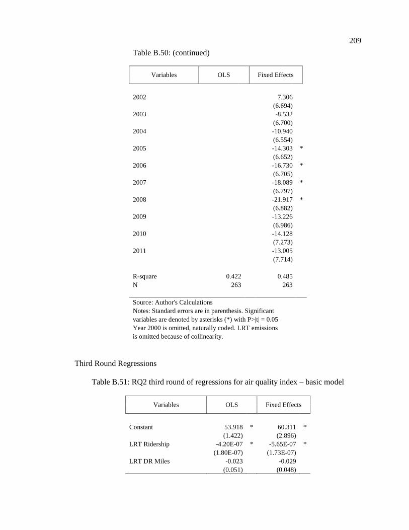
209
Table B.50: (continued)
Variables OLS Fixed Effects
2002 7.306(6.694)
2003 -8.532(6.700)
2004 -10.940(6.554)
2005 -14.303 *(6.652)
2006 -16.730 *(6.705)
2007 -18.089 *(6.797)
2008 -21.917 *(6.882)
2009 -13.226(6.986)
2010 -14.128(7.273)
2011 -13.005(7.714)
R-square 0.422 0.485N 263 263
Source: Author's CalculationsNotes: Standard errors are in parenthesis. Significantvariables are denoted by asterisks (*) with P>|t| = 0.05Year 2000 is omitted, naturally coded. LRT emissionsis omitted because of collinearity.
Third Round Regressions
Table B.51: RQ2 third round of regressions for air quality index – basic model
Variables OLS Fixed Effects
Constant 53.918 * 60.311 *(1.422) (2.896)
LRT Ridership -4.20E-07 * -5.65E-07 *(1.80E-07) (1.73E-07)
LRT DR Miles -0.023 -0.029(0.051) (0.048)
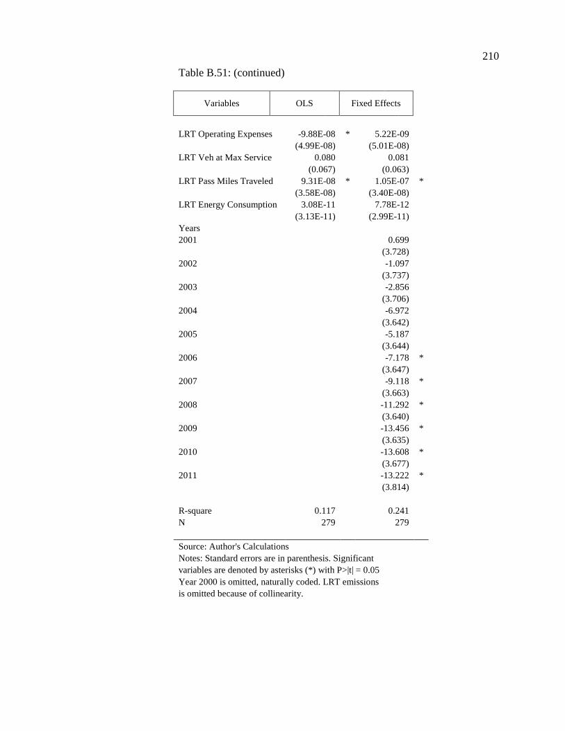
210
Table B.51: (continued)
Variables OLS Fixed Effects
LRT Operating Expenses -9.88E-08 * 5.22E-09(4.99E-08) (5.01E-08)
LRT Veh at Max Service 0.080 0.081(0.067) (0.063)
LRT Pass Miles Traveled 9.31E-08 * 1.05E-07 *(3.58E-08) (3.40E-08)
LRT Energy Consumption 3.08E-11 7.78E-12(3.13E-11) (2.99E-11)
Years2001 0.699
(3.728)2002 -1.097
(3.737)2003 -2.856
(3.706)2004 -6.972
(3.642)2005 -5.187
(3.644)2006 -7.178 *
(3.647)2007 -9.118 *
(3.663)2008 -11.292 *
(3.640)2009 -13.456 *
(3.635)2010 -13.608 *
(3.677)2011 -13.222 *
(3.814)
R-square 0.117 0.241N 279 279
Source: Author's CalculationsNotes: Standard errors are in parenthesis. Significantvariables are denoted by asterisks (*) with P>|t| = 0.05Year 2000 is omitted, naturally coded. LRT emissionsis omitted because of collinearity.
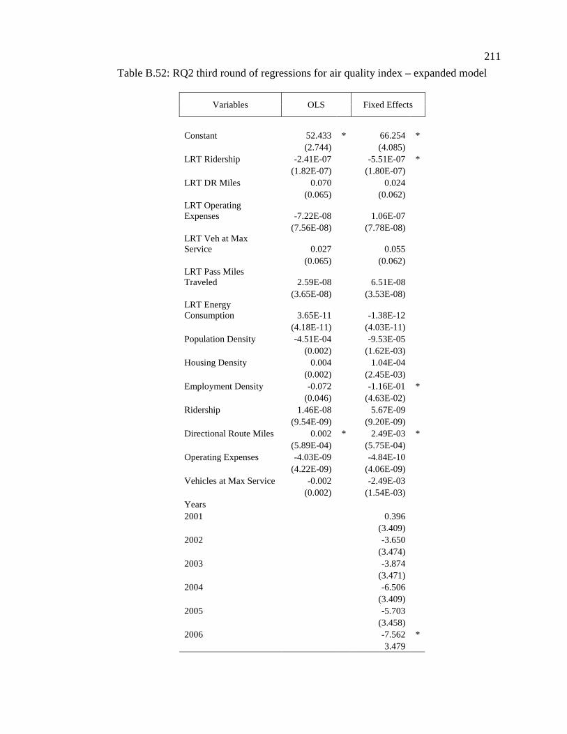
211
Table B.52: RQ2 third round of regressions for air quality index – expanded model
Variables OLS Fixed Effects
Constant 52.433 * 66.254 *(2.744) (4.085)
LRT Ridership -2.41E-07 -5.51E-07 *(1.82E-07) (1.80E-07)
LRT DR Miles 0.070 0.024(0.065) (0.062)
LRT OperatingExpenses -7.22E-08 1.06E-07
(7.56E-08) (7.78E-08)LRT Veh at MaxService 0.027 0.055
(0.065) (0.062)LRT Pass MilesTraveled 2.59E-08 6.51E-08
(3.65E-08) (3.53E-08)LRT EnergyConsumption 3.65E-11 -1.38E-12
(4.18E-11) (4.03E-11)Population Density -4.51E-04 -9.53E-05
(0.002) (1.62E-03)Housing Density 0.004 1.04E-04
(0.002) (2.45E-03)Employment Density -0.072 -1.16E-01 *
(0.046) (4.63E-02)Ridership 1.46E-08 5.67E-09
(9.54E-09) (9.20E-09)Directional Route Miles 0.002 * 2.49E-03 *
(5.89E-04) (5.75E-04)Operating Expenses -4.03E-09 -4.84E-10
(4.22E-09) (4.06E-09)Vehicles at Max Service -0.002 -2.49E-03
(0.002) (1.54E-03)Years2001 0.396
(3.409)2002 -3.650
(3.474)2003 -3.874
(3.471)2004 -6.506
(3.409)2005 -5.703
(3.458)2006 -7.562 *
3.479
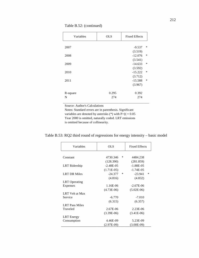
212
Table B.52: (continued)
Variables OLS Fixed Effects
2007 -9.537 *(3.519)
2008 -12.076 *(3.541)
2009 -14.633 *(3.592)
2010 -15.222 *(3.712)
2011 -15.588 *(3.967)
R-square 0.295 0.392N 274 274
Source: Author's CalculationsNotes: Standard errors are in parenthesis. Significantvariables are denoted by asterisks (*) with P>|t| = 0.05Year 2000 is omitted, naturally coded. LRT emissionsis omitted because of collinearity.
Table B.53: RQ2 third round of regressions for energy intensity – basic model
Variables OLS Fixed Effects
Constant 4730.346 * 4484.238(128.390) (281.859)
LRT Ridership -2.48E-05 -1.88E-05(1.71E-05) -1.74E-05
LRT DR Miles -24.377 * -23.941 *(4.816) (4.832)
LRT OperatingExpenses 1.16E-06 -2.67E-06
(4.73E-06) (5.02E-06)LRT Veh at MaxService -6.770 -7.010
(6.315) (6.357)LRT Pass MilesTraveled 2.67E-06 2.23E-06
(3.39E-06) (3.41E-06)LRT EnergyConsumption 4.46E-09 5.23E-09
(2.97E-09) (3.00E-09)
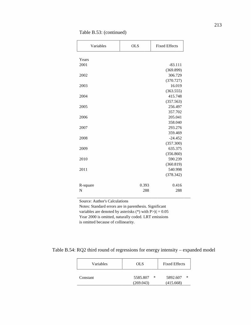
213
Table B.53: (continued)
Variables OLS Fixed Effects
Years2001 -83.111
(369.899)2002 306.729
(370.727)2003 16.019
(363.555)2004 415.748
(357.563)2005 256.497
357.7022006 205.041
358.0402007 293.276
359.4692008 -24.452
(357.300)2009 635.375
(356.860)2010 590.239
(360.819)2011 540.998
(378.342)
R-square 0.393 0.416N 288 288
Source: Author's CalculationsNotes: Standard errors are in parenthesis. Significantvariables are denoted by asterisks (*) with P>|t| = 0.05Year 2000 is omitted, naturally coded. LRT emissionsis omitted because of collinearity.
Table B.54: RQ2 third round of regressions for energy intensity – expanded model
Variables OLS Fixed Effects
Constant 5585.807 * 5892.607 *(269.043) (415.668)
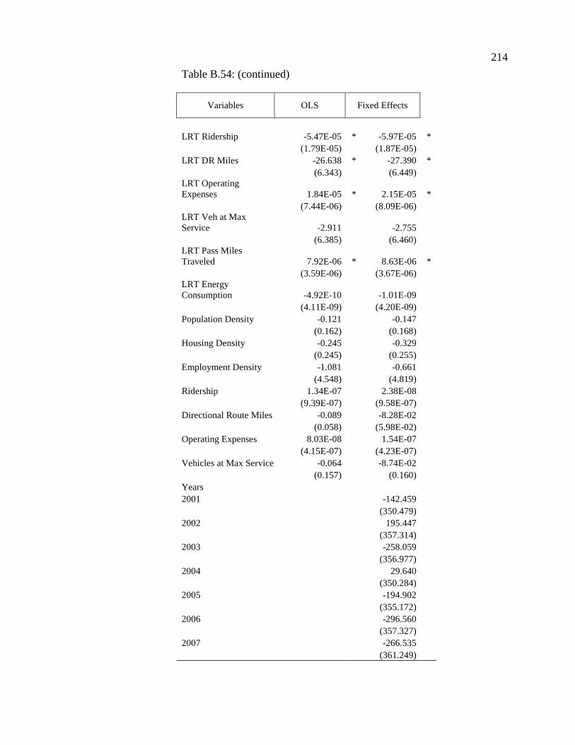
214
Table B.54: (continued)
Variables OLS Fixed Effects
LRT Ridership -5.47E-05 * -5.97E-05 *(1.79E-05) (1.87E-05)
LRT DR Miles -26.638 * -27.390 *(6.343) (6.449)
LRT OperatingExpenses 1.84E-05 * 2.15E-05 *
(7.44E-06) (8.09E-06)LRT Veh at MaxService -2.911 -2.755
(6.385) (6.460)LRT Pass MilesTraveled 7.92E-06 * 8.63E-06 *
(3.59E-06) (3.67E-06)LRT EnergyConsumption -4.92E-10 -1.01E-09
(4.11E-09) (4.20E-09)Population Density -0.121 -0.147
(0.162) (0.168)Housing Density -0.245 -0.329
(0.245) (0.255)Employment Density -1.081 -0.661
(4.548) (4.819)Ridership 1.34E-07 2.38E-08
(9.39E-07) (9.58E-07)Directional Route Miles -0.089 -8.28E-02
(0.058) (5.98E-02)Operating Expenses 8.03E-08 1.54E-07
(4.15E-07) (4.23E-07)Vehicles at Max Service -0.064 -8.74E-02
(0.157) (0.160)Years2001 -142.459
(350.479)2002 195.447
(357.314)2003 -258.059
(356.977)2004 29.640
(350.284)2005 -194.902
(355.172)2006 -296.560
(357.327)2007 -266.535
(361.249)
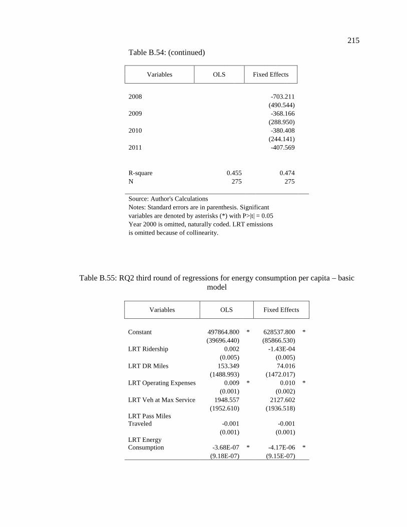
215
Table B.54: (continued)
Variables OLS Fixed Effects
2008 -703.211(490.544)
2009 -368.166(288.950)
2010 -380.408(244.141)
2011 -407.569
R-square 0.455 0.474N 275 275
Source: Author's CalculationsNotes: Standard errors are in parenthesis. Significantvariables are denoted by asterisks (*) with P>|t| = 0.05Year 2000 is omitted, naturally coded. LRT emissionsis omitted because of collinearity.
Table B.55: RQ2 third round of regressions for energy consumption per capita – basicmodel
Variables OLS Fixed Effects
Constant 497864.800 * 628537.800 *(39696.440) (85866.530)
LRT Ridership 0.002 -1.43E-04(0.005) (0.005)
LRT DR Miles 153.349 74.016(1488.993) (1472.017)
LRT Operating Expenses 0.009 * 0.010 *(0.001) (0.002)
LRT Veh at Max Service 1948.557 2127.602(1952.610) (1936.518)
LRT Pass MilesTraveled -0.001 -0.001
(0.001) (0.001)LRT EnergyConsumption -3.68E-07 * -4.17E-06 *
(9.18E-07) (9.15E-07)
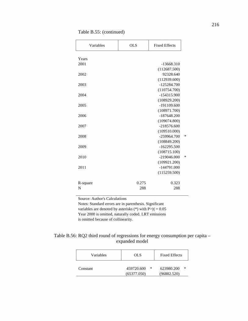
216
Table B.55: (continued)
Variables OLS Fixed Effects
Years2001 -13668.310
(112687.500)2002 92328.640
(112939.600)2003 -125284.700
(110754.700)2004 -154315.900
(108929.200)2005 -191109.600
(108971.700)2006 -187648.200
(109074.800)2007 -218576.600
(109510.000)2008 -259964.700 *
(108849.200)2009 -162295.500
(108715.100)2010 -219046.000 *
(109921.200)2011 -144791.000
(115259.500)
R-square 0.275 0.323N 288 288
Source: Author's CalculationsNotes: Standard errors are in parenthesis. Significantvariables are denoted by asterisks (*) with P>|t| = 0.05Year 2000 is omitted, naturally coded. LRT emissionsis omitted because of collinearity.
Table B.56: RQ2 third round of regressions for energy consumption per capita –expanded model
Variables OLS Fixed Effects
Constant 459720.600 * 623980.200 *(65377.050) (96882.520)
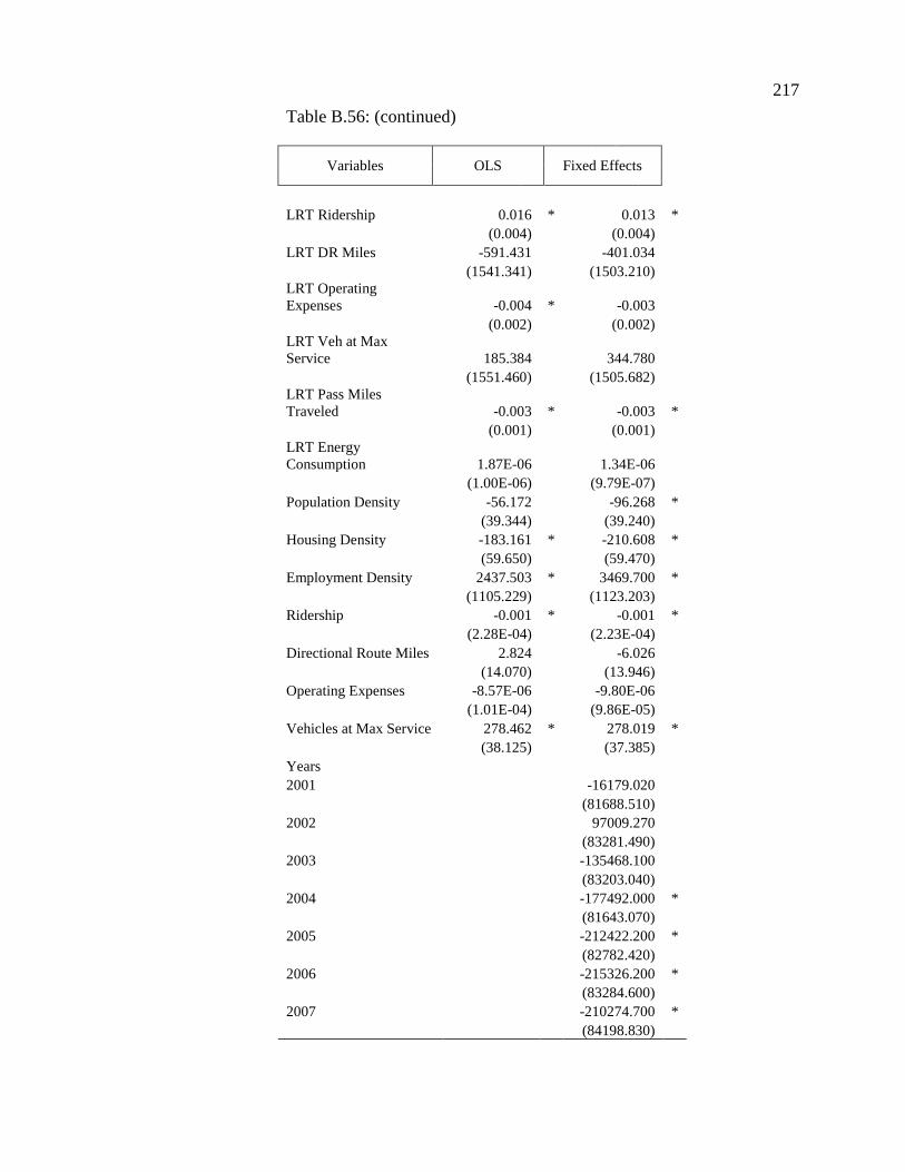
217
Table B.56: (continued)
Variables OLS Fixed Effects
LRT Ridership 0.016 * 0.013 *(0.004) (0.004)
LRT DR Miles -591.431 -401.034(1541.341) (1503.210)
LRT OperatingExpenses -0.004 * -0.003
(0.002) (0.002)LRT Veh at MaxService 185.384 344.780
(1551.460) (1505.682)LRT Pass MilesTraveled -0.003 * -0.003 *
(0.001) (0.001)LRT EnergyConsumption 1.87E-06 1.34E-06
(1.00E-06) (9.79E-07)Population Density -56.172 -96.268 *
(39.344) (39.240)Housing Density -183.161 * -210.608 *
(59.650) (59.470)Employment Density 2437.503 * 3469.700 *
(1105.229) (1123.203)Ridership -0.001 * -0.001 *
(2.28E-04) (2.23E-04)Directional Route Miles 2.824 -6.026
(14.070) (13.946)Operating Expenses -8.57E-06 -9.80E-06
(1.01E-04) (9.86E-05)Vehicles at Max Service 278.462 * 278.019 *
(38.125) (37.385)Years2001 -16179.020
(81688.510)2002 97009.270
(83281.490)2003 -135468.100
(83203.040)2004 -177492.000 *
(81643.070)2005 -212422.200 *
(82782.420)2006 -215326.200 *
(83284.600)2007 -210274.700 *
(84198.830)
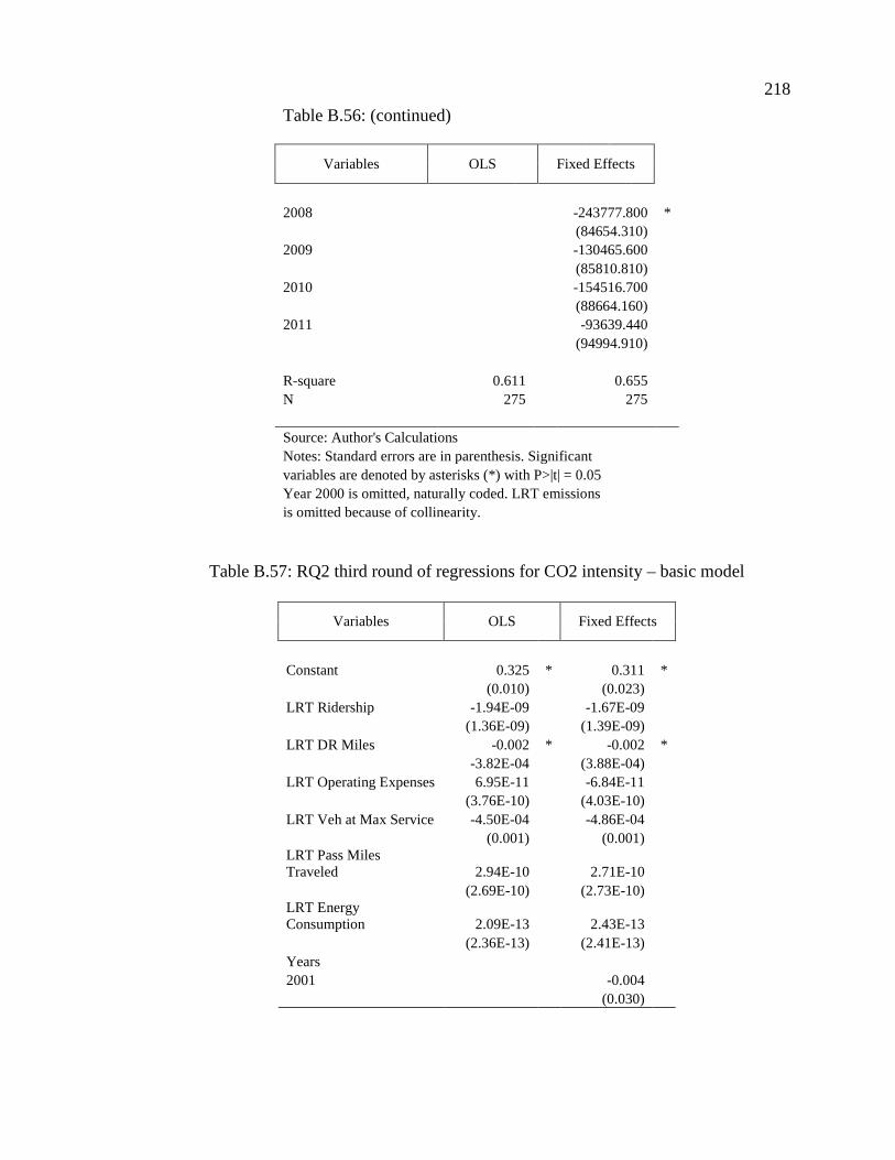
218
Table B.56: (continued)
Variables OLS Fixed Effects
2008 -243777.800 *(84654.310)
2009 -130465.600(85810.810)
2010 -154516.700(88664.160)
2011 -93639.440(94994.910)
R-square 0.611 0.655N 275 275
Source: Author's CalculationsNotes: Standard errors are in parenthesis. Significantvariables are denoted by asterisks (*) with P>|t| = 0.05Year 2000 is omitted, naturally coded. LRT emissionsis omitted because of collinearity.
Table B.57: RQ2 third round of regressions for CO2 intensity – basic model
Variables OLS Fixed Effects
Constant 0.325 * 0.311 *(0.010) (0.023)
LRT Ridership -1.94E-09 -1.67E-09(1.36E-09) (1.39E-09)
LRT DR Miles -0.002 * -0.002 *-3.82E-04 (3.88E-04)
LRT Operating Expenses 6.95E-11 -6.84E-11(3.76E-10) (4.03E-10)
LRT Veh at Max Service -4.50E-04 -4.86E-04(0.001) (0.001)
LRT Pass MilesTraveled 2.94E-10 2.71E-10
(2.69E-10) (2.73E-10)LRT EnergyConsumption 2.09E-13 2.43E-13
(2.36E-13) (2.41E-13)Years2001 -0.004
(0.030)
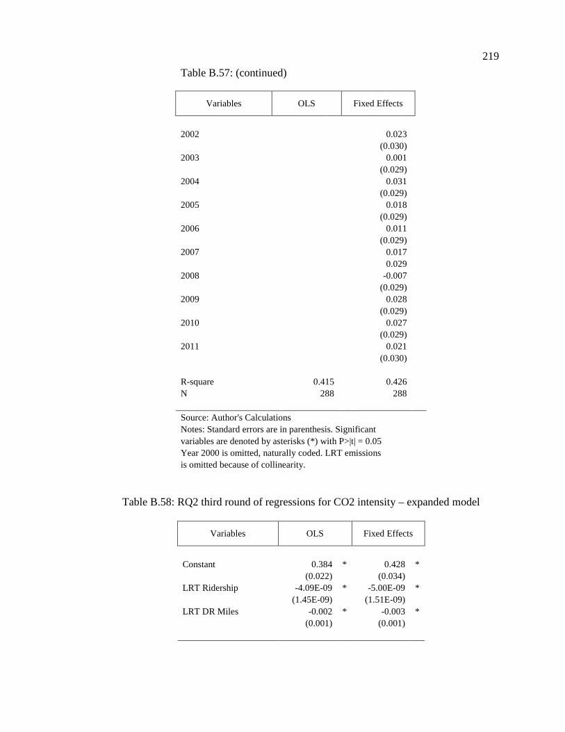
219
Table B.57: (continued)
Variables OLS Fixed Effects
2002 0.023(0.030)
2003 0.001(0.029)
2004 0.031(0.029)
2005 0.018(0.029)
2006 0.011(0.029)
2007 0.0170.029
2008 -0.007(0.029)
2009 0.028(0.029)
2010 0.027(0.029)
2011 0.021(0.030)
R-square 0.415 0.426N 288 288
Source: Author's CalculationsNotes: Standard errors are in parenthesis. Significantvariables are denoted by asterisks (*) with P>|t| = 0.05Year 2000 is omitted, naturally coded. LRT emissionsis omitted because of collinearity.
Table B.58: RQ2 third round of regressions for CO2 intensity – expanded model
Variables OLS Fixed Effects
Constant 0.384 * 0.428 *(0.022) (0.034)
LRT Ridership -4.09E-09 * -5.00E-09 *(1.45E-09) (1.51E-09)
LRT DR Miles -0.002 * -0.003 *(0.001) (0.001)
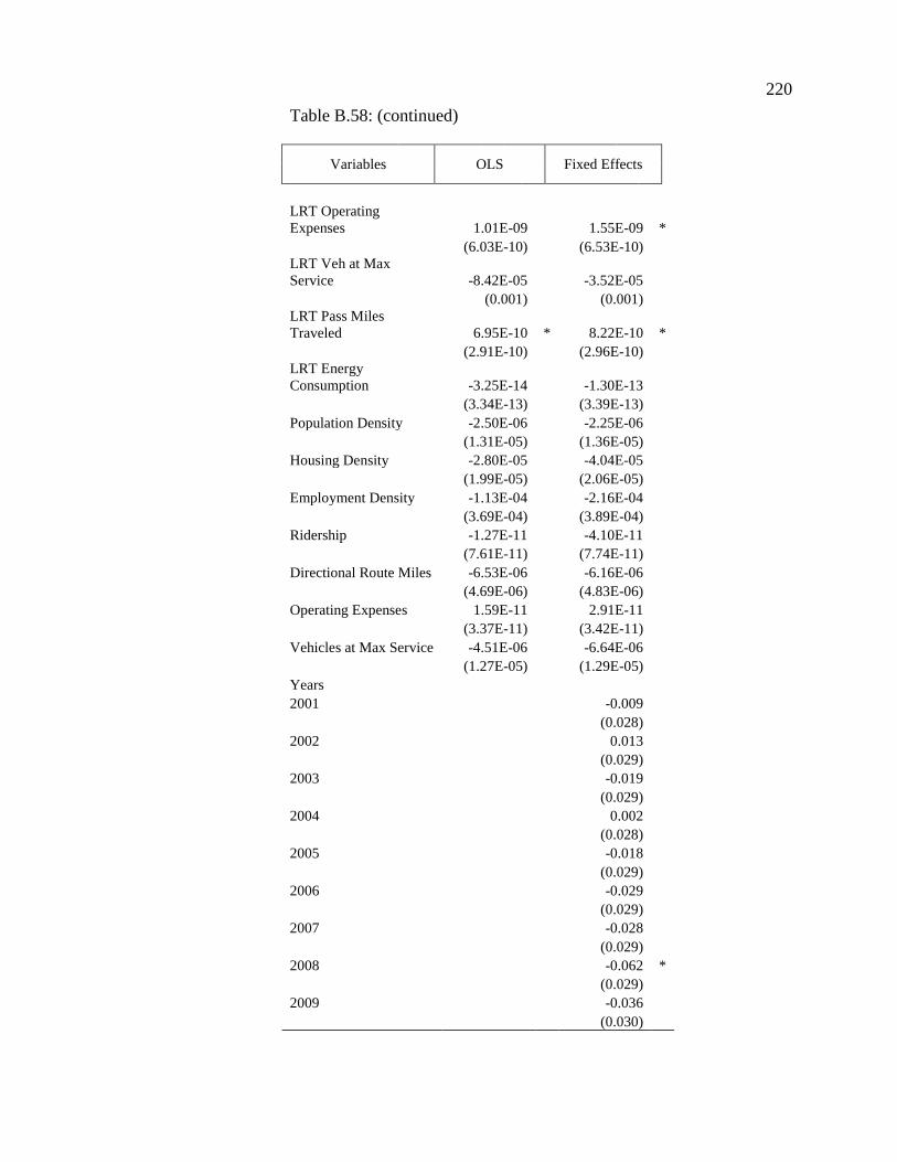
220
Table B.58: (continued)
Variables OLS Fixed Effects
LRT OperatingExpenses 1.01E-09 1.55E-09 *
(6.03E-10) (6.53E-10)LRT Veh at MaxService -8.42E-05 -3.52E-05
(0.001) (0.001)LRT Pass MilesTraveled 6.95E-10 * 8.22E-10 *
(2.91E-10) (2.96E-10)LRT EnergyConsumption -3.25E-14 -1.30E-13
(3.34E-13) (3.39E-13)Population Density -2.50E-06 -2.25E-06
(1.31E-05) (1.36E-05)Housing Density -2.80E-05 -4.04E-05
(1.99E-05) (2.06E-05)Employment Density -1.13E-04 -2.16E-04
(3.69E-04) (3.89E-04)Ridership -1.27E-11 -4.10E-11
(7.61E-11) (7.74E-11)Directional Route Miles -6.53E-06 -6.16E-06
(4.69E-06) (4.83E-06)Operating Expenses 1.59E-11 2.91E-11
(3.37E-11) (3.42E-11)Vehicles at Max Service -4.51E-06 -6.64E-06
(1.27E-05) (1.29E-05)Years2001 -0.009
(0.028)2002 0.013
(0.029)2003 -0.019
(0.029)2004 0.002
(0.028)2005 -0.018
(0.029)2006 -0.029
(0.029)2007 -0.028
(0.029)2008 -0.062 *
(0.029)2009 -0.036
(0.030)
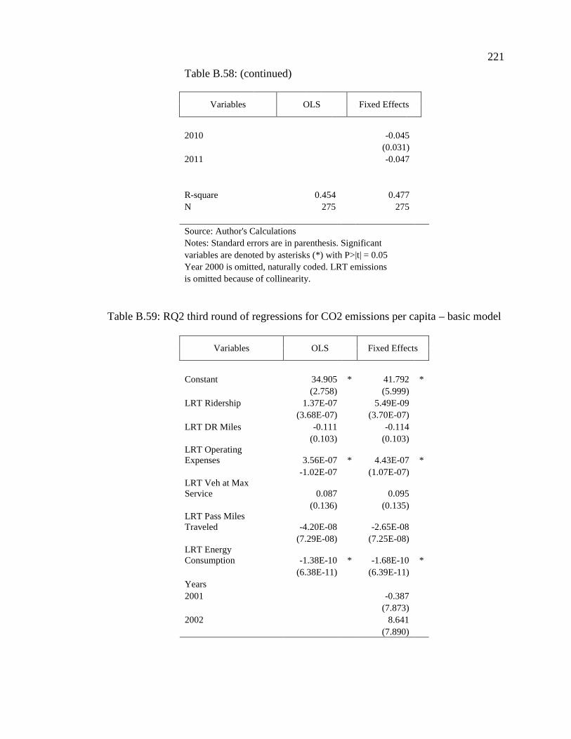
221
Table B.58: (continued)
Variables OLS Fixed Effects
2010 -0.045(0.031)
2011 -0.047
R-square 0.454 0.477N 275 275
Source: Author's CalculationsNotes: Standard errors are in parenthesis. Significantvariables are denoted by asterisks (*) with P>|t| = 0.05Year 2000 is omitted, naturally coded. LRT emissionsis omitted because of collinearity.
Table B.59: RQ2 third round of regressions for CO2 emissions per capita – basic model
Variables OLS Fixed Effects
Constant 34.905 * 41.792 *(2.758) (5.999)
LRT Ridership 1.37E-07 5.49E-09(3.68E-07) (3.70E-07)
LRT DR Miles -0.111 -0.114(0.103) (0.103)
LRT OperatingExpenses 3.56E-07 * 4.43E-07 *
-1.02E-07 (1.07E-07)LRT Veh at MaxService 0.087 0.095
(0.136) (0.135)LRT Pass MilesTraveled -4.20E-08 -2.65E-08
(7.29E-08) (7.25E-08)LRT EnergyConsumption -1.38E-10 * -1.68E-10 *
(6.38E-11) (6.39E-11)Years2001 -0.387
(7.873)2002 8.641
(7.890)
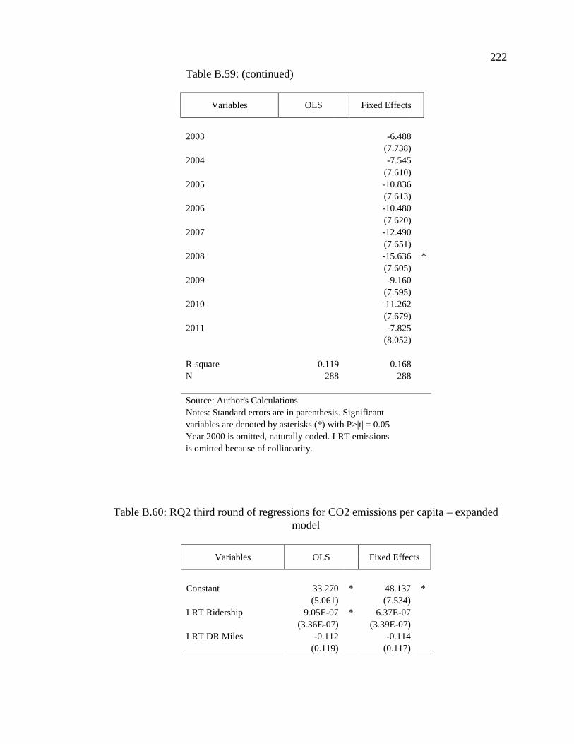
222
Table B.59: (continued)
Variables OLS Fixed Effects
2003 -6.488(7.738)
2004 -7.545(7.610)
2005 -10.836(7.613)
2006 -10.480(7.620)
2007 -12.490(7.651)
2008 -15.636 *(7.605)
2009 -9.160(7.595)
2010 -11.262(7.679)
2011 -7.825(8.052)
R-square 0.119 0.168N 288 288
Source: Author's CalculationsNotes: Standard errors are in parenthesis. Significantvariables are denoted by asterisks (*) with P>|t| = 0.05Year 2000 is omitted, naturally coded. LRT emissionsis omitted because of collinearity.
Table B.60: RQ2 third round of regressions for CO2 emissions per capita – expandedmodel
Variables OLS Fixed Effects
Constant 33.270 * 48.137 *(5.061) (7.534)
LRT Ridership 9.05E-07 * 6.37E-07(3.36E-07) (3.39E-07)
LRT DR Miles -0.112 -0.114(0.119) (0.117)
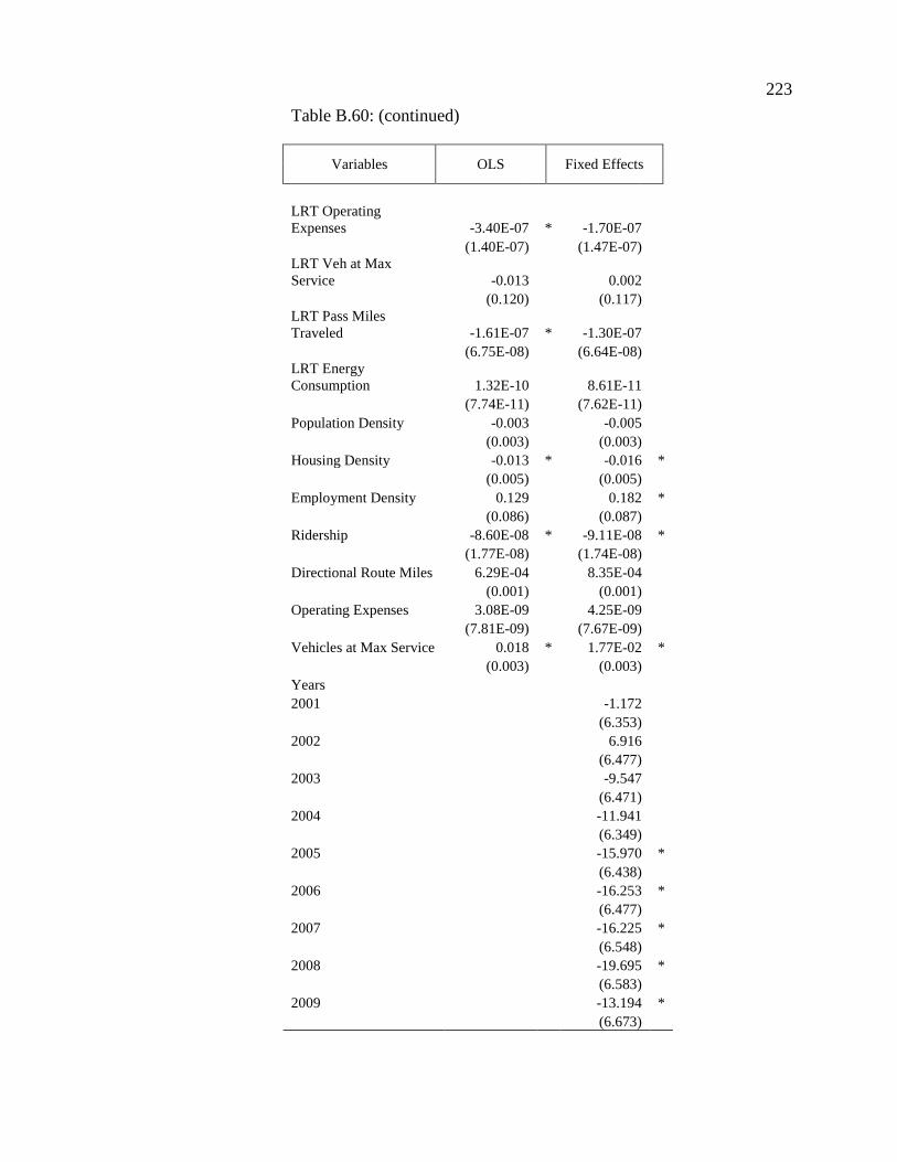
223
Table B.60: (continued)
Variables OLS Fixed Effects
LRT OperatingExpenses -3.40E-07 * -1.70E-07
(1.40E-07) (1.47E-07)LRT Veh at MaxService -0.013 0.002
(0.120) (0.117)LRT Pass MilesTraveled -1.61E-07 * -1.30E-07
(6.75E-08) (6.64E-08)LRT EnergyConsumption 1.32E-10 8.61E-11
(7.74E-11) (7.62E-11)Population Density -0.003 -0.005
(0.003) (0.003)Housing Density -0.013 * -0.016 *
(0.005) (0.005)Employment Density 0.129 0.182 *
(0.086) (0.087)Ridership -8.60E-08 * -9.11E-08 *
(1.77E-08) (1.74E-08)Directional Route Miles 6.29E-04 8.35E-04
(0.001) (0.001)Operating Expenses 3.08E-09 4.25E-09
(7.81E-09) (7.67E-09)Vehicles at Max Service 0.018 * 1.77E-02 *
(0.003) (0.003)Years2001 -1.172
(6.353)2002 6.916
(6.477)2003 -9.547
(6.471)2004 -11.941
(6.349)2005 -15.970 *
(6.438)2006 -16.253 *
(6.477)2007 -16.225 *
(6.548)2008 -19.695 *
(6.583)2009 -13.194 *
(6.673)
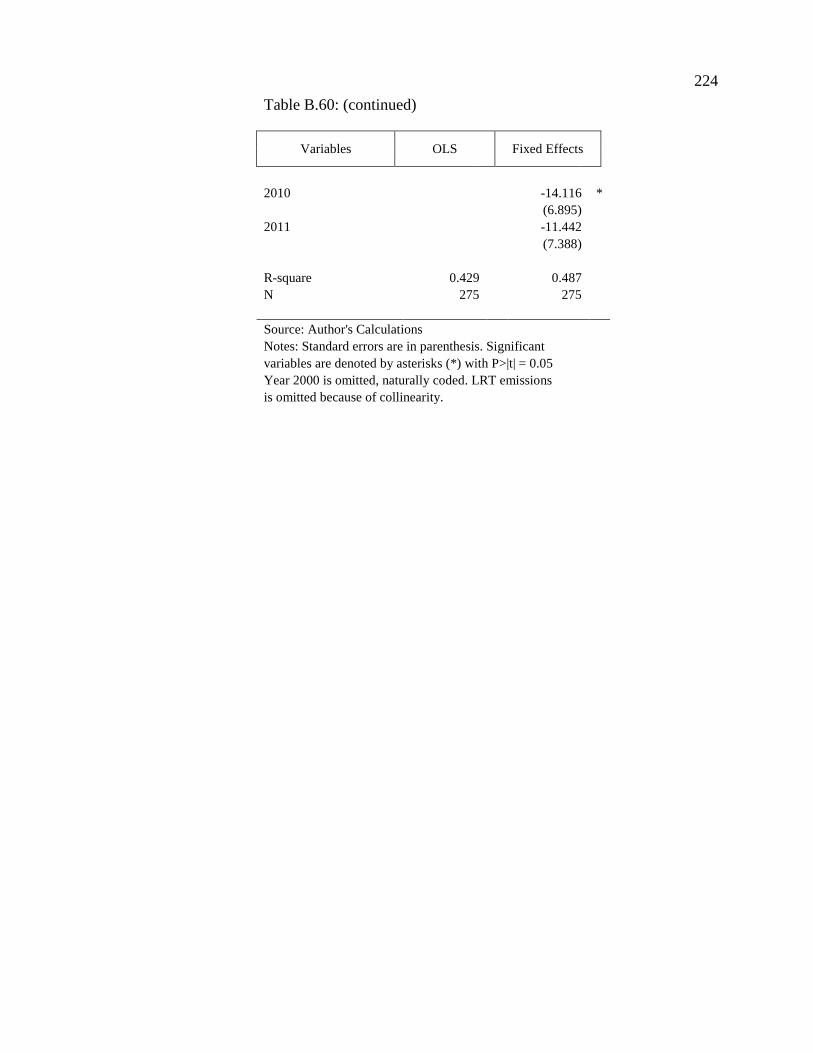
224
Table B.60: (continued)
Variables OLS Fixed Effects
2010 -14.116 *(6.895)
2011 -11.442(7.388)
R-square 0.429 0.487N 275 275
Source: Author's CalculationsNotes: Standard errors are in parenthesis. Significantvariables are denoted by asterisks (*) with P>|t| = 0.05Year 2000 is omitted, naturally coded. LRT emissionsis omitted because of collinearity.