Environmental monitoring: between science and decision-making

J. Richir, S. Gobert, P.

Lejeune, G. Watson and

Ph. Grosjean

CIBIM

13-04-2016

Mons

Trace elements

(after Amiard, 2011)

Bioindicator : Posidonia oceanica

Michel, 2012

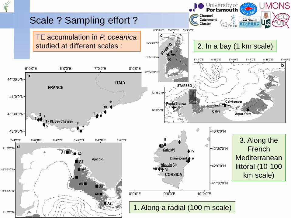
Scale ? Sampling effort ?

TE accumulation in P. oceanica

studied at different scales :

1. Along a radial (100 m scale)

2. In a bay (1 km scale)

3. Along the

French

Mediterranean

littoral (10-100

km scale)

Scale ? Sampling effort ?

4. Along the whole Mediterranean coastline (100-1000 km scale)

TE accumulation in P. oceanica

studied at different scales :

Scale ? Sampling effort ?

1. Along a radial (100 m)

2. In a bay (1 km)

3. Along the French littoral (10-100 km)

4. Along the Mediterranean coastline (100-1000 km)

Conclusion

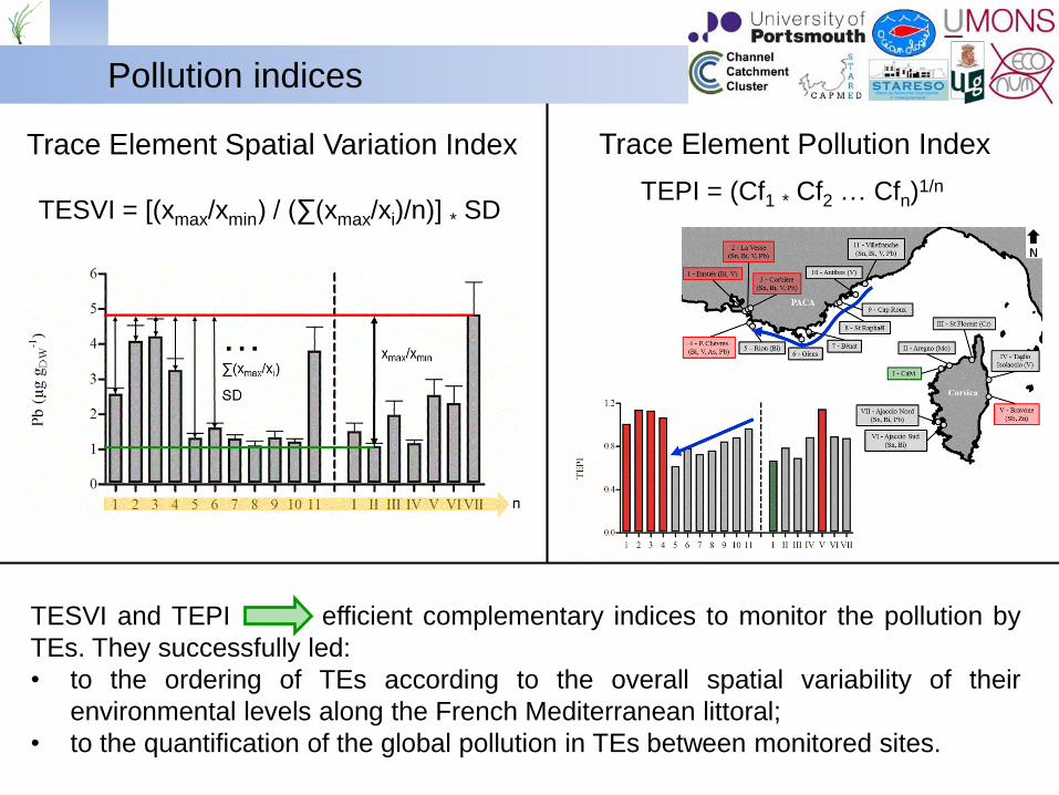
Trace Element Spatial Variation Index

TESVI = [(xmax/xmin) / (∑(xmax/xi)/n)] * SD

Trace Element Pollution Index

TEPI = (Cf1 * Cf2 … Cfn)1/n

TESVI and TEPI efficient complementary indices to monitor the pollution by

TEs. They successfully led:

• to the ordering of TEs according to the overall spatial variability of their

environmental levels along the French Mediterranean littoral;

• to the quantification of the global pollution in TEs between monitored sites.

Pollution indices

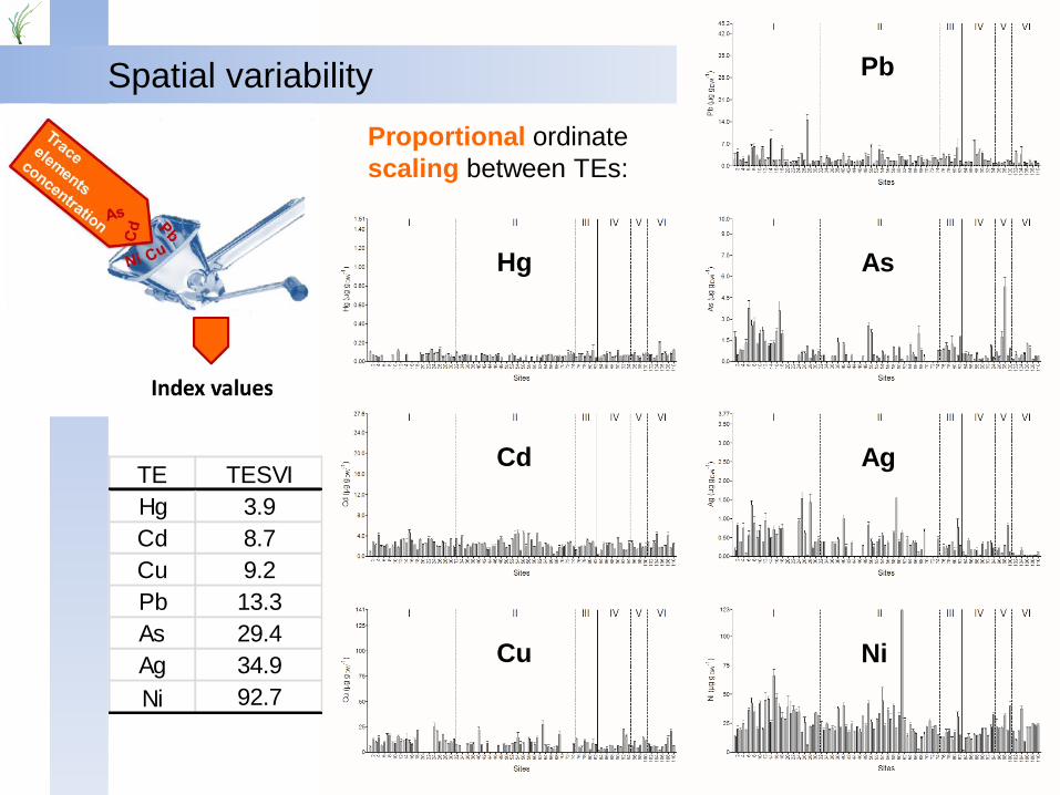
Spatial variability

Proportional ordinate

scaling between TEs:

Hg

Cd

Cu

As

Ag

Ni

Pb

TE TESVI

Hg 3.9

Cd 8.7

Cu 9.2

Pb 13.3

As 29.4

Ag 34.9

Ni 92.7

Global contamination

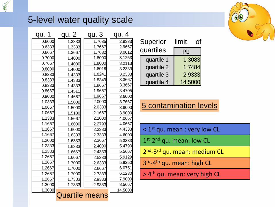
5-level water quality scale

0.6000

0.6333

0.6667

0.7000

0.7667

0.8000

0.8333

0.8333

0.8333

0.8667

0.9000

1.0333

1.0667

1.0667

1.1333

1.1667

1.1667

1.1667

1.2000

1.2333

1.2333

1.2667

1.2667

1.2667

1.2667

1.2667

1.3000

1.3000

1.3333

1.3333

1.3667

1.4000

1.4000

1.4000

1.4333

1.4333

1.4333

1.4511

1.4667

1.5000

1.5000

1.5180

1.5667

1.6000

1.6000

1.6333

1.6333

1.6333

1.6667

1.6667

1.7000

1.7000

1.7000

1.7333

1.7333

1.7635

1.7667

1.7682

1.8000

1.8000

1.8018

1.8241

1.8349

1.8667

1.9667

1.9667

2.0000

2.0333

2.1667

2.2000

2.2793

2.3333

2.3333

2.3667

2.4000

2.4333

2.5333

2.6333

2.6667

2.7333

2.9333

2.9333

2.9333

2.9667

3.0012

3.1253

3.2113

3.2333

3.2333

3.3667

3.3667

3.4705

3.6000

3.7667

3.8000

3.9000

4.0667

4.0667

4.4333

4.6000

5.3333

5.4790

5.5667

5.9129

5.9250

6.0751

6.1230

7.9000

8.5667

14.5000

Ag As Cd Cu Hg Ni Pb

quartile 1 0.1833 0.4000 1.8283 6.4500 0.0552 17.9250 1.3083

quartile 2 0.3667 0.6333 2.2996 8.5667 0.0663 22.2833 1.7484

quartile 3 0.5642 1.2333 2.8292 12.6263 0.0798 31.5852 2.9333

quartile 4 1.5500 5.3000 4.6714 27.7000 0.2041 123.0000 14.5000

Ag As Cd Cu Hg Ni Pb

quartile 1 0.1833 0.4000 1.8283 6.4500 0.0552 17.9250 1.3083

quartile 2 0.3667 0.6333 2.2996 8.5667 0.0663 22.2833 1.7484

quartile 3 0.5642 1.2333 2.8292 12.6263 0.0798 31.5852 2.9333

quartile 4 1.5500 5.3000 4.6714 27.7000 0.2041 123.0000 14.5000

Superior limit of

quartiles

qu. 1 qu. 2 qu. 3 qu. 4

Quartile means

< 1st qu. mean : very low CL

1st-2nd qu. mean: low CL

2nd-3rd qu. mean: medium CL

3rd-4th qu. mean: high CL

> 4th qu. mean: very high CL

5 contamination levels

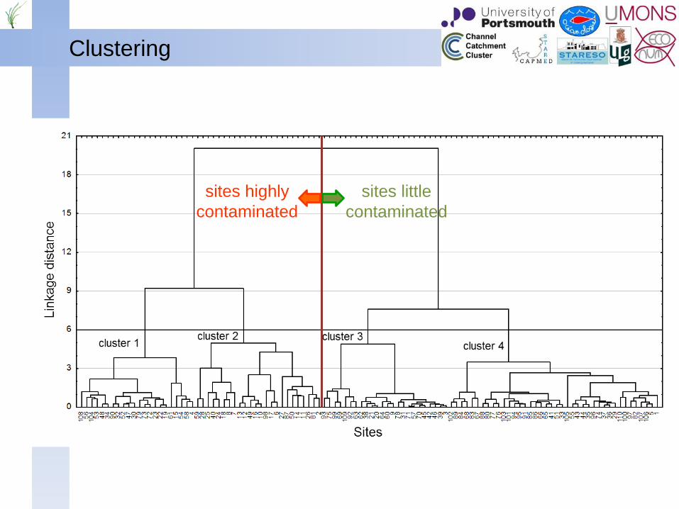
Clustering

sites highly

contaminated

sites little

contaminated

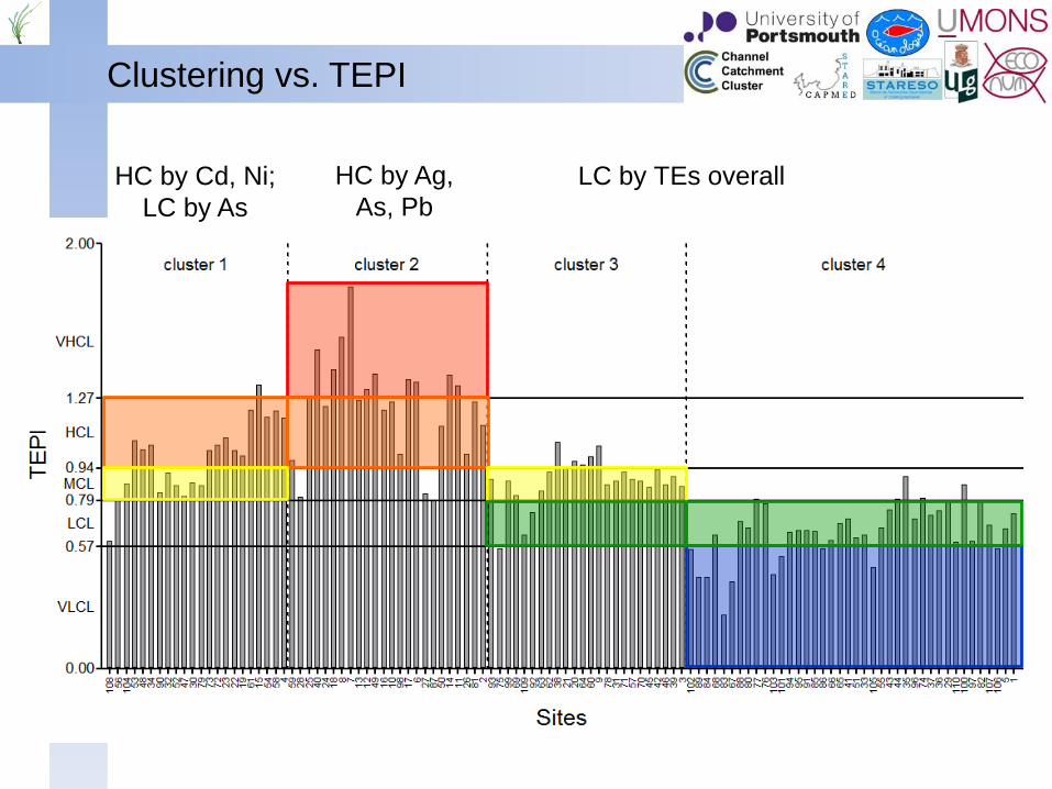
HC by Cd, Ni;

LC by As

HC by Ag,

As, Pb

LC by TEs overall

Clustering vs. TEPI

Posidonia oceanica: shoots,

rhizomes and roots;

• Foliar stratum ◄ water;

• Matte ◄ sediments.

Posidonia oceanica bed

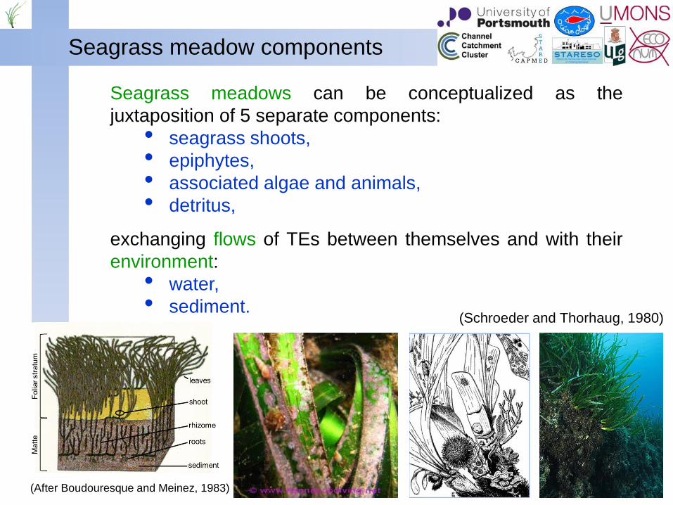
Seagrass meadow components

Seagrass meadows can be conceptualized as the

juxtaposition of 5 separate components:

• seagrass shoots,

• epiphytes,

• associated algae and animals,

• detritus,

exchanging flows of TEs between themselves and with their

environment:

• water,

• sediment.

(After Boudouresque and Meinez, 1983)

(Schroeder and Thorhaug, 1980)

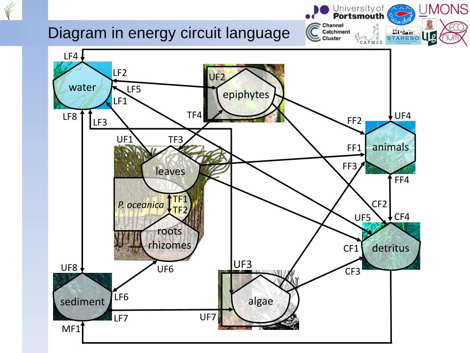
P. oceanica

leaves

rootsrhizomes

waterepiphytes

sediment algae

detritus

animalsUF1

LF1

TF1TF2

TF3

TF4

LF6

UF2LF2

UF3

LF3LF8

UF8

LF4

UF5

LF5

UF4

FF1

FF2

FF3

FF4

CF4CF2

CF3

CF1

MF1

UF6

LF7 UF7

Diagram in energy circuit language

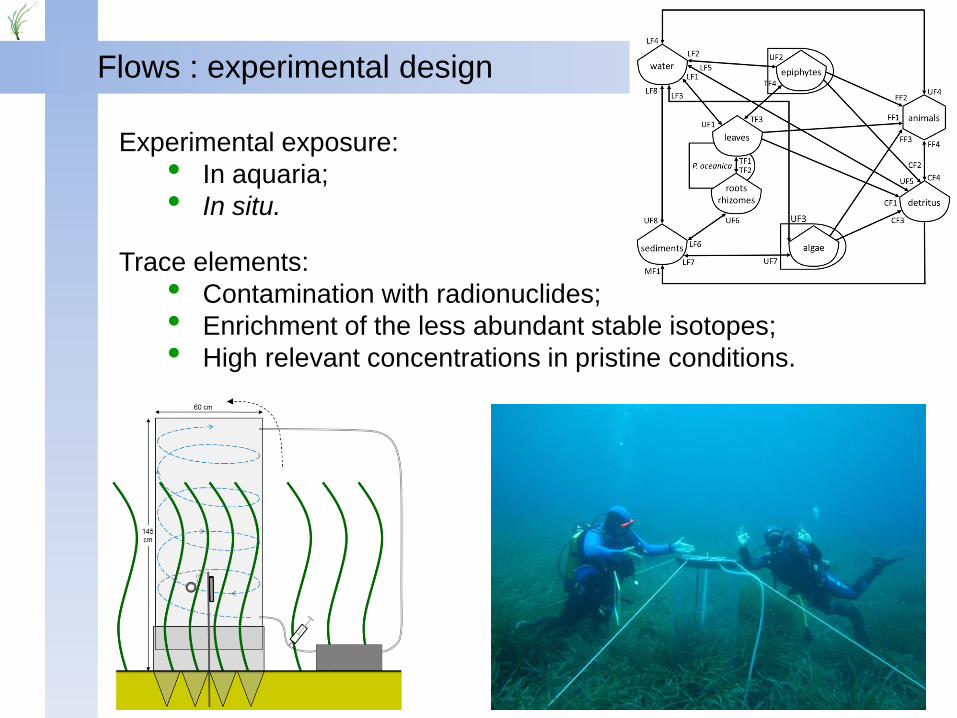
Flows : experimental design

Experimental exposure:

• In aquaria;

• In situ.

Trace elements:

• Contamination with radionuclides;

• Enrichment of the less abundant stable isotopes;

• High relevant concentrations in pristine conditions.

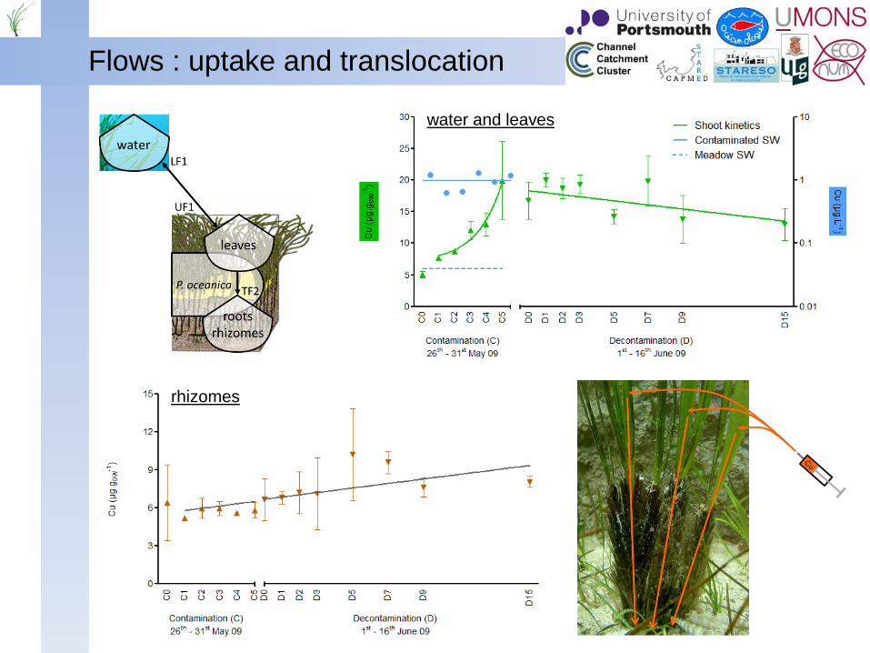
Flows : uptake and translocation

water and leaves

rhizomes

TEs in seagrass meadows

Data compilation for the different components of the model;

Mass balance analyses;

Experiments.

The quantification of the role played by P. oceanica

meadows in the coastal biogeochemistry of TEs and their

function of biological filter.

M. galloprovincialis monitoring station

©Ifremer

Applications

A

P

P

L

I

C

A

T

I

O

N

S

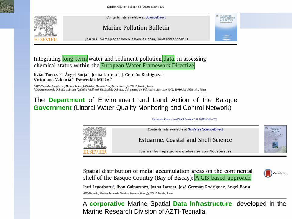
The Department of Environment and Land Action of the Basque

Government (Littoral Water Quality Monitoring and Control Network)

A corporative Marine Spatial Data Infrastructure, developed in the

Marine Research Division of AZTI-Tecnalia

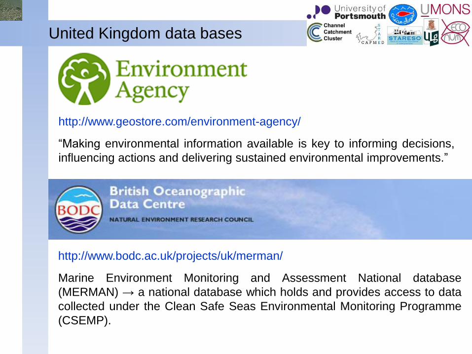
United Kingdom data bases

http://www.geostore.com/environment-agency/

“Making environmental information available is key to informing decisions,

influencing actions and delivering sustained environmental improvements.”

http://www.bodc.ac.uk/projects/uk/merman/

Marine Environment Monitoring and Assessment National database

(MERMAN) → a national database which holds and provides access to data

collected under the Clean Safe Seas Environmental Monitoring Programme

(CSEMP).

PORTSMOUTH

SOUTHAMPTON

0

100

200

300

1/01

/199

2

1/01

/199

4

1/01

/199

6

1/01

/199

8

1/01

/200

0

1/01

/200

2

1/01

/200

4

1/01

/200

6

1/01

/200

8

1/01

/201

0

1/01

/201

2

1/01

/201

4

BL

TEL

PELZ

n (

mg

kg

DW

-1);

< 6

3 µ

m

0

20

40

60

80

100

100

200

1/01

/199

2

1/01

/199

4

1/01

/199

6

1/01

/199

8

1/01

/200

0

1/01

/200

2

1/01

/200

4

1/01

/200

6

1/01

/200

8

1/01

/201

0

1/01

/201

2

1/01

/201

4

TEL

BL

PEL

Pb

(m

g k

gD

W-1

); <

63

µm

8

32

128

512

2048

1/01

/199

2

1/01

/199

4

1/01

/199

6

1/01

/199

8

1/01

/200

0

1/01

/200

2

1/01

/200

4

1/01

/200

6

1/01

/200

8

1/01

/201

0

1/01

/201

2

1/01

/201

4

BLTEL

PEL

log

2 C

u (

mg

kg

DW

-1);

< 6

3 µ

m0.0

0.5

1.0

1.5

1/01

/199

2

1/01

/199

4

1/01

/199

6

1/01

/199

8

1/01

/200

0

1/01

/200

2

1/01

/200

4

1/01

/200

6

1/01

/200

8

1/01

/201

0

1/01

/201

2

1/01

/201

4

LODTEL

PEL

Hg

(m

g k

gD

W-1

); <

63

µm

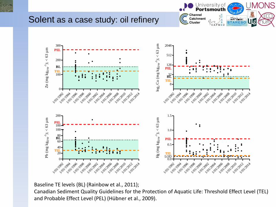
Solent as a case study: oil refinery

Baseline TE levels (BL) (Rainbow et al., 2011);Canadian Sediment Quality Guidelines for the Protection of Aquatic Life: Threshold Effect Level (TEL)and Probable Effect Level (PEL) (Hübner et al., 2009).

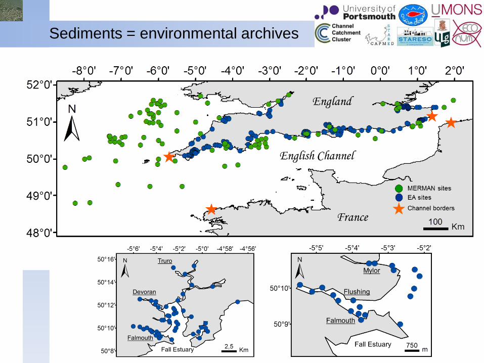
Sediments = environmental archives

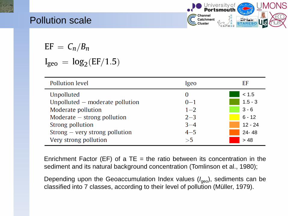
Pollution scale

Enrichment Factor (EF) of a TE = the ratio between its concentration in the

sediment and its natural background concentration (Tomlinson et al., 1980);

Depending upon the Geoaccumulation Index values (Igeo), sediments can be

classified into 7 classes, according to their level of pollution (Müller, 1979).

2

< 1.5

1.5 - 3

3 - 6

6 - 12

12 - 24

24- 48

> 48

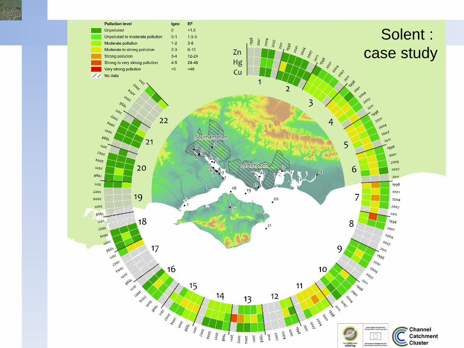
Solent :

case study

Data mining - Decision tools - Monitoring

Long-term sediment pollution data:

assessment of the chemical

status within the European WFD;

Knowledge transfer from scientists to

environmental managers:

develop practical environmental

management tools;

Complementary monitoring approach:

environmental compartments

vs. biota.

Questions?

… Thank you for your attention …