Environmental Modelling and Expert Fuzzy Control of Climate in a Miniature Cropping

House

Damon Berry BSc (Eng), Dip. E.E.

Submitted for the Award of MSc July 1996

Supervisor: Dr. Richard Hayes

Department of Control Systems and ElectricalEngineering

DIT Kevin St. Dublin 8

For Grandad The Quiet Man

Thanks to all those who advised and supported the author during this work

Special thanks to my supervisor, Richard Hayes

You know who you

I hereby Certify that this material which I now submit for assessment on the programme of study leading to the award of MSc is entirely my own work and has not been taken from the work of others save and to the extent that such work has been cited and acknowledged within the text of my work

n,»

Environmental Modelling and Expert Fuzzy Control of Climate in a Miniature Cropping House

Damon Berry BSc (Eng), Dip E E

Project AbstractThis work describes the development o f an inexpensive control system for a miniature cropping house which uses the method o f crop production

The control system was first developed in the Matlab-Simulink environment where it controlled a simulated model o f the plant The model was composed o f four differential equations describing, air temperature in the cropping house, water temperature, C 0 2 concentration and inside humidity I he controller comprises a fuzzy “expert” controller which accepts inputs o f light intensity and air temperature and returns fan speed and water temperature set-point as outputs The latter was applied as a set-point for digital PID controller which controls water temperature in the cropping house

Expert advice, as well as knowledge o f the plant gained from observation ol the plant and the model, were used to develop fuzzy sets and a fuzzy rule-base The controller was implemented in Matlab simulation language and tested on the model o f the plant

Finally, the controller was implemented in “C” source and assembly for a standalone Motorola 68HC11 microprocessor based digital controller Development o f software for the micro-controller was conducted using the Motorola’s Evaluation Tool-kit PCBUG The controller circuits included two temperature sensing circuits, a light input and power control circuitry for both a DC fan and a set o f aquarium heaters

Table of Contents

I 1 B a c k g r o u n d t o t i ie D e v h o p m e n t o r ri ic C o n t r o i S y s te m f o r i h f C r o p p in g \ lo i isi I1 2 T in M a ih e m a t ic a i M o o n o r m i C i im a t i W i i i i i n i h i C r o p p in g I l o u s i 2I 3 U s in g a C o m p u t e r t o C o n t r o l i h e E n v ir o n m e n t w it h in a G r l i n m o u s i 21 4 S u m m a r y o f t h e C o n t e n t s o r m is T h e s is 3CHAPTER 2 HYDROPONICS 62 1 In t r o d u c t io n 62 2 A e r ia l E n v ir o n m e n t 6

2 2 1 The Effects o f Air Temperature on the Growth o f Plants 72 2 2 Cooling the Air by Ventilation 72 2 3 Using Glazing to Reduce Heat Losses 8

2 2 4 Control o f Carbon Dioxide Levels within a Greenhouse 92 3 C o n t r o l o f t h e R h iz o s p h e r e 12

2 3 1 The Nutrient Film Technique 122 3 2 The Water Supply in an NFT System 142 3 3 Mineral Requirements o f Plants 152 3 4 The Effects o f Root Zone Wanning 162 3 5 The Needfor an Adequate Oxygen Supply to Roots 172 3 6 Other Considerations 17

2 4 R e v ie w o f L im its a n d O p tim u m V a l u e s o f P a r a m e t e r s in a n N F T C o n t r o l S y s t e m 18CHAPTER 3 FUZZY LOGIC CONTROL 203 1 A n In t r o d u c t io n t o F u z z y L o g ic C o n t r o l 2 03 2 In t r o d u c t io n t o F u z z y Lo g ic 2 13 3 FUZZiriCATION 223 4 iNrERENCING 243 5 D e f u z z if ic a t io n 28

3 5 1 Height Defuzzification 283 5 2 Centroid Defuzzification 28

3 6 T h e R e a s o n t o r U s in g F u z z y L o g ic in E n v i r o n m e n t a l C o n t r o l 293 7 F u z z y L o g ic a n d E x p e r t C o n t r o l 303 8 F u r i i irR R e a d in g 31CHAPTER 4 MODEL OF MINIATURE CROPPING HOUSE 324 I In t r o d u c t io n 324 2 T Y P r s o r M a t h e m a t ic a l M o d e l s u s l d Fo r D e s c r ib in g E n v i r o n m e n t S y s i f m s 334 3 C o n t r o i i f d V a r ia b l e s in a C o m m f r c ia l H y d r o p o n ic s -B a s e d C r o p p in g S y s i f m 344 4 Di v l l o p m l n r o r i i ie D c i l r m i n i s i ic M o d e l o i a n NFT C r o p p in g S y s i i m 364 5 A s s u m p t io n s t o r D e t e r m in is t ic M o d f l o f M in ia t u r f C r o p p in g H o u s i 384 6 L q u a i io n s D l s c r i b i n g E n v i r o n m l n i w i i i iin N F I - B a s e d Vi g i i a b i i C r o p p in g I lo u s i 394 7 H e a t a n d M a s s T r a n s f e r M e c h a n is m s in G l a s s h o u s e s 4 0

4 7 1 Short Wave Radiation 404 7 3 Long Wave Radiation 414 7 4 Conduction 424 7 5 Ventilation 434 7 6 Convection and the Diffusion oj Heat 444 7 7 Evaporation Transpiration and Condensation 454 7 8 C 0 2 Assimilation by Plants 484 8 D e r iv a t io n o f M o d e l o f C ro p p in g Housr 504 8 1 Heat Balance in Internal Air in the Cropping House 504 8 2 Heat Balance at Nutrient Solution and Plant Canopy Sutface 514 8 3 Moisture Mass Balance at Inside Air 52

CHAPTER 1 INTRODUCTION 1

v

4 8 4 C02 Mass Balance in inside Air 534 9 D e v e l o p m e n t o f t h e M o d e l o r t h e C r o p p in g H o u s e in t h e M a i l a b -S im u l in k S im u i a i io n E n v ir o n m e n t 544 10 S t e a d y S t a t e C h a r a c t e r is t ic s o f t h e D e t e r m in is t ic M o d e l o r ti i r C r o p p in g H o u s i 55

4 IO I Steady State Chat acteristic o f the inside Air Temperatili e 554 10 2 Steady State Nutrient Solution Temperatiti e Chat act et tsdcs 574 / 3 3 Steady State Inside Absolute Humidity Characteristics 594 10 4 Steady State Inside C 0 2 Concentration Characteristic 60

4 11 S u m m a r y o f C h a p t e r 4 63CHAPTER 5 MODEL VALIDATION BY COMPARISON WITH REAL SYSTEM 635 I In t r o d u c t io n 63 5 2 U s in g R e a l H is t o r ic a l D a t a to A s s e s s t h e P l r i o r m a n c e o i im l C r o p p in g H o u s i M o d i i 63

5 2 1 Data-Logger and Instrumentation 645 2 2 Configuration o f Data Logging Equipment fo r the Data-logging Experiment and Other Boundary Conditions 6 6

5 3 D y n a m ic R e s p o n s e s o r t h e D if f e r e n t ia l Eq u a tio n s D e s c r ib in g C o n d i i io n s In s id l i i ii C r o p p in g H o u s l 69

5 3 1 Dynamic Responses o f the Air and Nutrient solution heat Balance Equations 695 3 2 Dynamic Response o f the Water Vapour Mass balance Equation 775 3 3 Dynamic Response o f the CO 2 Mass balance Equation 79

5 4 U s in g ti ie M o d e l t o D e t e r m in e t h e S ig n if ic a n c e o r H e a t T r a n s f e r s w iti un ti i r C r o p p in g H o u s e 815 6 S u m m a r y or C h a p t e r 5 83CHAPTER 6 CONTROL SYSTEM FOR VEGETABLE PROPAGATION UNIT 846 1 In t r o d u c t io n 846 2 T i ie C o n s t r u c t io n a n d O p e r a tion o r ti ie V e g e t a b l e P r o p a g a t io n U n it 86

6 2 1 Description o f the Vegetable Propagation Unit 8 6

6 2 2 Ventilation o f the Vegetable Propagation Unit 8 8

6 2 3 Nutrient Recirculation in the Vegetable Propagation Unit 8 8

6 2 4 Nutrient Flow within a Tray 896 2 5 Heating o f Recirculated Nutrient Solution 91

5 3 MC68HC11 MICROCONTROLLER UNIT 926 3 1 Summary o f the Elements the 68HC11-Based Digital Controller 926 3 2 Overview o f the 68HC11 Micro-controller 946 3 3 Using the 68HC11 as a Standalone Micro-controller 966 3 4 Sampling o f Temperature and Light Intensity 966 3 5 Serial Communications to the P C 976 3 6 Using Pulse Width Modulation to Control Fan Speed 98

6 4 CON IROLLLR INS! RUMEN IA HON AND CON I ROI O U IPU I CIRCUI IS 9 86 4 1 dc - dc Converter 996 4 2 Over- Voltage Protection 996 4 3 Micro-controller Operating Frequency 1016 4 4 Temperature Sensing Circuit 1016 4 5 Light Sensor 1036 4 6 Control Output fo r Heater 1036 4 7 Control Output fo r Fan Current 1046 4 8 The Complete Micro-controller System 105

6 5 THE SOFTWARE DEVELOPMENT SYSTEM FOR THE DIGITAL ENVIRONMENTAI CONTROLl ER 1056 6 C o n t r o l l e r S o f t w a r e 107

6 6 1 Introduction 1076 6 2 Direct Digital Control o f Nutrient Solution Tempei ature 1086 6 3 Control o f Aerial Environment Using Fuzzy Logic 110

6 7 SIMULATION OF THE COMPLETE CONTROL SYSTEM 1 156 7 1 Description o f the Simulated Control System as Implemented in Matlab/Simuhnk 1166 7 2 Response o f the Simulated Controller to Step Changes in External Air Temperature 118

6 8 Im p l e m e n t a t io n 011 n r C o n i ro i l e r to r im e 6 8 H C 1 1 M ic r o -c o n t r o i i t r 1226 8 1 Sequence o f Operation o f Controller Code 123

VI

6 8 2 Execution time and Memory Requirements fo r the Control! er 1236 8 3 Other Comments on the implementation and Testing o f the Controller 124

6 9 P e r f o r m a n c e T r i a l s o r t h e E x p e r t F u z z y C o n i r o l l e r o n T iir R e a l S y s te m a n d o n n ii S im u la ! l d S y s t e m 125

6 9 1 Controller Performance Trial on the Real System 1256 9 2 Controller Performance Ti ¡al on Simulation oj the Cr opping House 129

6 10 S u m m a r y 130CHAPTER 7 DISCUSSION 1317 I IN I RODUCI ION 1317 2 DISCUSSION OF PERrORMANCF OF TI IE MODEL OF TI IE CROPPING HOUSI 13 1

7 2 1 General Performance o f the Deterministic Model 1317 2 2 The Heat Balance Equation for Nutrient Solution 1327 2 3 The Heat Balance Equation fo r the Air Inside the Cr opping Home 1337 2 4 The Water Vapour Mass Balance Equation for the Air Inside the Cropping House 1347 2 4 The C 0 2 Mass Balance Equation 1357 2 5 Suggested Improvements to the Data-loggmg System 136

7 3 ASSL SSMLNI Ol 11IL Pi Rl ORMANU 01 MIL CON IROI IJ R 1377 4 RrcoMMENDrD I m p r o v e m e n t s i o C o n t r o i i f r 140

7 4 1 Extra Sensors as Inputs jo r the Digital Controller 1407 4 2 Suggestions fo r Additional Control Outputs 1427 4 3 Other Additions to the Controller Hardware and Software 144

CHAPTER 8 CONCLUSION 1478 1 In t r o d u c t io n 1478 2 T h e D e t e r m in is t ic m o d e l o f t h e C r o p p in g H o u s e 1478 3 T m C l im a t e C o n i r o i i i r i o r ih f C r o p p in g I lo u s i 148APPENDIX A ADDITIONAL EXPERIMENTAL RESULTS iA l F a n C h a r a c t e r is t ic s i

APPENDIX B SOFTWARE LISTINGS AND FLOWCHARTS iB l 68HC11 M em o ry M ap iB 2 Fi owcmarts tor Low i rvri Routines ivAPPENDIX C PARAMETERS USED IN MODEL OF CROPPING HOUSE iC 1 V a r i a b l e s in M o d e l a n d V a l u e s o i P a r a m e t e r s t o r O r i g i n a i M o d e l iC 2 V a i u r s o r P A R A M r T r R s w h i c h W F R rC i iA N G rD io R M o D in r o M o d i i h i

APPENDIX D EXTRA CALCULATIONS IE l C a l c u l a i i o n o f t h e L in e a r A p p r o x i m a t i o n o i t h e R a t e o i N l i Lo n g W a v e R a d i a i i o n E m i s s i o n s f r o m t h e C r o p C a n o p y a n d N ut r ie n r S u r f a c e i

APPENDIX E REFERENCES i

VH

Table of Figures

CHAPTER 2 6Fig 2 1 Thermal and Optical Properties o f Various Cover Mat et ¡als 9Fig 2 2 A Modern Commercial High Volume NFT Cropping System 13

CHAPTER 3 20Fig 3 1 Elements o f a Fuzzy Logic Controller 20Fig 3 2 Fuzzification o f a Crisp Measurement Using Tt iangular Sets 22Fig 3 2 Fuzzification Using Sfunction Membership Functions 24Fig 3 4 Min and Product Inferencing 26Fig 3 5 Generation o f a Fuzzy Control Surface Using Product inferencing 27

CHAPTER 4 32Fig 4 1 Block Diagram o f Model o f Miniature Cropping House 37Fig 4 2 Diffusion o f C 0 2 into the chloroplasts 49Fig 4 3 The Cropping House Showing Heat Flows 52Fig 4 4 The Cropping House Showing Moisture Flows 53Fig 4 5 The Cropping House Showing C 0 2 Flows 54Fig 4 6 Simuhnk Block Diagram Showing the Cropping House with Changeable Inputs andDisplaying Model Outputs 55Fig 4 7 Steady State Inside Air Temperature Versus Ventilation Rate fo r Different WaterTemperatures with Outside Air Temperature at 0°C, and heater power at 400 W 56Ftg4 8 Steady State Nutrient Temperature Versus External Air Temperature for Different HeateiPowers with the Inside Air Temperature in That mal Equilibrium with (he Temperature of the Nutrient 58Tig 4 9 Steady State Inside Absolute Humidity Versus Ventilation Rate fo r Different ExternalAbsolute Humidities 59Fig 4 10 Steady State Inside C 0 2 Concentration Versus Ventilation Rate for Different Levels o fIncident Solar Radiation 6 1Fig 4 11 Steady State Inside C 0 2 Concentration Versus Ventilation Rate for Dijfet ent MesophyllC 0 2 Concentrations 6 1

CHAPTER 1 1

CHAPTER 5 63Fig 5 1 The Cropping House with Conti oiler and Data-Logger 64Fig 5 2 Measured Response o f Air Temperature Inside the Cropping House to External Conditions Between the 16th and 19th o f September 1994 and the Response oj the Original Model to Input Data Collected Over the Same Time Period 71Tig 5 3 Measured Response o f Nutrient Solution Tempet atui e in the Ci opptng House to Extei nal Conditions Between the 16th and 19,h o f September 1994 and the Response o f the Original Model to Input Data Collected Over the Same Time Period 72Fig 5 4 Measured Response o f Air Temperature in (he Cropping House to External Conditions Between the 16th and I9,h o f September 1994 and the Response o f the Modified Model to Input Data Collected Over the Same Time Pet lod 73Fig 5 5 Measured Response o f Nutrient Solution Temperature in the Real System to ExternalConditions Between the I 6 lh and 19th o f September 1994 and the Response o f the Modified Model to Input Data Collected Over the Same Time Period 74Fig 5 6 Measured Response o f Nutrient Solution Temperature In the Cr opping House to a StepChange in Heater Power o f 0 to 400W on 16th September ¡994 and the Modelled Response o f the Nutrient Tempet ature in the Modified Model with Input Data Collected Over the Same Time Period 75Tig 5 7 Measwed Response of Inside An 7tm puatu ie in the Cropping House to a Step Change in Heater Power o f 0 to 400W on 16th September 1994 and the Modelled Response of the Inside Air Temperature in the Modified Model with Input Data Collected Over the Same lim e Period 76

VIII

Fig 5 8 Measured Response of Inside Relative Humidity m the Real System to External ConditionsBetween the I6'h and !9'h o f September 1994 and the Response o f the Original Model to Input Data Collected During this Time 77Fig 5 9 Measured Response o f Inside Relative Humidity in (he Real System to External Conditions Between the 16th and 19,h o f September 1994 and the Response o f the Modified Model to Input Data Collected During this Time 78Fig 5 10 The Measured CO2 concentration withm the Miniature Cropping House On the 2 T ‘September 1994 and the Response o f the Model with Input Data Collected Ovei the Same Time Period 80

CHAPTER 6 84Tig 6 1 Block Diagram o f Conti ol System fo r the Miniature Cropping Home 85Fig 6 2 Nutrient Flow in the Vegetable Propagation Unit and in a Single Ti ay 90Fig 6 3 Simplified representation o f Digital Controller Hardware 93Fig 6 4 Features o f The 68HC/ /E9 Micro Controller Unit 95Tig 6 5 Block Diagram o f the Cn ants for the Environmental Conti oiler 99Fig 6 6 Over- Voltage Protection Circuit fo r dc-dc Converter 100Fig 6 7 Temperatw e Sensing Circuit 102Fig 6 8 MCU Output Circuit fo r Controlling Heater Cut rent 103Fig 6 9 MCU Output Circuit fo r Controlling Fan Speed 105Fig 6 10 The Software Development System fo r the 68HCI1-Based Environmental Controller 106Fig 6 11 Input and Output Universes o f Discourse fo r Expert Fuzzy> Controller 113Fig 6 12 Simuhnk Block Diagram Showing the Complete Conti ol system fo r the Ci opping Houseand Displaying Model Outputs 116Fig 6 13 Simuhnk Block Diagram representation o f the Simuhnk group ADC which Models anAnalogue to Digital Converter 118

Tig 6 14 Simulated Responses o f Controlled Nutnent Tempuatuie to Step Changes m External AnTemperature 119Fig 6 15 Simulated Responses o f Controlled Inside Air Temperature to Step Changes in ExternalA ir Temperature 121Fig 6 16 Sequence o f Execution o f Controller code 123Fig 6 17 Controller Performance Chart from the 3rtl to the 7lh June 1995 Showing the Variation o f Inside Air Temperature and Nutnent Solution Temperature over the Four Day Period In Response to Changes m the Air Temperature Outside the Cropping House 126Fig 6 18 Response o f Inside Air Temperature and Nutrient temperature in the Tull Control System Model to Changes in Air Temperature over a Four Day Period During June 1995 with Humidity Unmeasured and Set at 80%RH 129

CHAPTER 7 131CHAPTER 8 146APPENDIX A 1Figure A 1 Static Characteristics o f the Papst D C Fan 11

APPENDIX B 1Fig B1 Memory Map o f the 68HC711E9 as Used in this Work 1Fig B 2 Memory Map o f Controller Parameters mFig B 3 Flowchart showing Relationship Between Low-level Routines and Controller Code ivrig B 4 Flowchart for Subroutine R7 UN I vTig B 5 Flowchart fo r Subr outine DECIS viFig B 6 Flowchart fo r Subroutine ADC vuFig B 7 Flowchart fo r the Subroutine SCI vinFig B 8 Flowchart fo r Subroutine PWMINI ixFig B 9 Flowchart fo r Subroutine P DECIS xFig BIO Flowchart fo r Subroutine CALOFF x

APPENDIX C

IX

APPENDIX D APPENDIX E

Table of Tables

CHAPTER 2 6Table 2 1 Limits fo r Controlled Parameters in an Environmental Control System for NTT 1<SI able 2 2 Limits and Preferred Values jo r Controlled Parameters in the Miniature Ct opprng

House 19CHAPTER 3 20CHAPTER 4 32CHAPTER 5 63Table 5 1 Heat Flows in the Cropping House 81

CHAPTER 6 84Table 6 I Controller Settings fo r Digital PJD Controller ¡09Table 6 2 Fuzzy Rule-base for Expert Fuzzy Climate Controller for Cropping House m TabularForm ¡¡5

CHAPTER 7 131CHAPTER 8 147APPENDIX A iAPPENDIX B iAPPENDIX C iAPPENDIX D iAPPENDIX E i

C HAPTER I I

XI

Chapter 1 Introduction

1.1 Background to the Development of the Control System for the Cropping House

The world population is increasing at a rate o f 320,000 per day One o f the principal problems created by this increase in world population is the difficulty in feeding everyone From 1950 to 1984, global food production tripled Since then, loss o f usable farmland has resulted in a levelling o ff in production (W orld Book 1993) This has resulted in a search for alternative and more resource-efficient methods o f growing food, such as hydroponics Hydroponics is a means o f growing plants using a solution o f nutrients in the place o f soil The advantage o f this technique is that the nutrient can be designed to meet each plants nutritional needs exactly, thus reducing the amount o f minerals and nitrates which are released into the surrounding environment In addition, because the plants receive an ideal mix of nutrient, they grow laster than those grown using conventional techniques O f course there is a price to pay for this extra productivity Hydroponics growth systems require energy to heat the nutrient solutions to a certain optimum temperature Consequently it is necessary to control the environment inside such cropping houses to conserve energy while keeping crop productivity high

The principal aim o f this work, is to develop a control system for a miniature hydroponic cropping house The control system will be expandable to allow additional controlled variables to be added at a later date it so required It will also to be inexpensive to produce and need the minimum o f attention by the grower Any aids to the growth of plants within the growing house will be automated where possible

1

This work will also present a deterministic mathematical model o f a miniature hydroponics-based growing house. This model is to be used in the development o f an environmental controller for the real system. The control system will be an expert system which uses existing growers’ knowledge to make decisions about ventilation and heating requirements o f the growing house.

1.2 The M athematical Model of the Climate Within the Cropping House

M odern research into new products often involves the use o f some form o f model either physical or mathematical, to assist understanding of the system being designed and to aid development work. A mathematical model o f the miniature cropping house was developed to fulfil these roles. The model was developed from consideration o f the physics o f the system. Since the model was developed from physical principles, the parameters affecting each variable in the model are transparent to the user. This allows these parameters to be changed easily, to test new designs involving different construction materials, cropping house dimensions or new control devices or control strategies.

1.3 Using a Computer to Control the Environment within a Greenhouse

The advantage o f using a computer-based or d i g i t a l controller for climate control in a greenhouse is that, in addition to performing all o f those functions performed by a standard hard-wired analogue climate controller, a digital controller can make decisions based on stage in cropping cycle, time o f day or time o f year. The configuration o f digital controllers is easily altered and this makes them very flexible. Vendors o f such controllers may easily have the software altered to suit changing control environments and to follow advances in control theory. For instance, many manufacturers o f commercial control systems have added modules which implement fuzzy logic control (M itsubishi,

2

M otorola) The hardware for these controllers is very similar if not identical to that required for conventional control techniques (M otorola 1993)

Growers rely to a large extent on their own experience when making decisions which affect the crop and the environment inside growing houses I heir reactions to changing environmental conditions inside and outside the growing house can be easily encapsulated in the rule-base o f a computer-based fuzzy logic controller (McDowell 1994, MacSioman 1994)

The computer-based environmental controller will accept as inputs, air temperature water temperature and light intensity It will control nutrient temperature by regulating the power to an electric water heater and will a!feet the aerial environment within the cropping house by controlling the power to a small d c fan

1 4 Summary of the Contents of this Thesis

This first chapter has given a brief introduction to the project and its various components

Chapter two will discuss the problems and control constraints associated with the development o f a hydroponic crop production system The information contained in this chapter is the expert knowledge which is used in the design of the expert fuzzy logic controller The chapter concludes with a table o f conditions which should be met for successful hydroponic crop production

Chapter three introduces fuzzy logic theory with an emphasis on its use in controllers An explanation o f the operation o f each stage o f a fuzzy logic engine is given with examples and diagrams

3

Chapter four will deal with the development o f a deterministic model of the cropping house It will describe the equations governing each o f the major processes affecting mass and heat flow within the cropping house and will show how these heat flows and mass flows can be balanced using four differential equations in addition it will present qualitative and quantitative validation o f the model

Chapter five shows the comparison between the response of the real cropping house to changing external climatic conditions and the response of the model with environmental data measured at the real system over the same time period It will reccomend changes which might improve the performance o f the model

Chapter six describes the construction and operation o f the miniature cropping house It also describes the elements of the control system lor the mimatuic cropping house These elements are as follows

• Controller instrumentation circuits• Control output circuits• The low-level service routines which perform the sampling and control the

PWM signals and serial communications• The controller code for the simulation o f the full control system and for the

micro-controller

Chapter seven discusses the results and findings o f the project and makes recommendations about possible improvements which could be made to the model and to the control system

Chapter eight is the conclusion

4

Appendix A contains additional experimental results, which are relevant to this work

Appendix B contains the memory map of the micro-controller unit and the flowcharts for the service routines for the micro-controller

Appendix C lists the parameters which were used in the model o f the cropping house and the values they take in the original model and the modifications made to improve the model’s performance

Appendix D derives an equation used in the work

Appendix E is the bibliography

5

Chapter 2: Hydroponics2.1 Introduction

This chapter outlines the Nutrient Film Technique (NFT) It also deals with the basic requirements and constraints ol an NFI system It lorms the basis lor the rule-based control approach developed in later chapters, by summarising some ol the control objectives in a linguistic lashion I he contiol problem may be broken into two distinct halves, the aerial environment and artificial root support and nutrition This chapter is partitioned accordingly I lie ilist part of the chapter deals with the aerial environment and discusses lactors in the design of a cropping system, which affect the content and temperature o f the air in the growing house and its interaction with the plant canopy I he second section deals with the factors influencing the behaviour o f the loot systems o f the plants

2.2 Aerial Environm ent

The control o f the temperature, moisture content and CO 2 concentration o f the air in greenhouses is desirable in colder climates to accelerate the growth ol plants Indeed the first recorded controlled environment for growing plants appears to be the growing oi oif-season cucumbers for the Emperor I lbcrius during the first century AD No significant advances were made in growing plants in an enclosed environment until greenhouses first appeared in 17th Century England Ihese houses were heated using fresh compost which decomposed producing a source ot CO 2 and heat (Jenson and Collins 1983)

Climate control is o f course also needed for hydroponics-based cropping houses This section discusses the ways in which the aerial environment aifects the growth o f plants in an N fT cropping system

2.2.1 The Effects o f Air Tem perature on the Growth o f Plants

Optimum air temperature values depend, as do many other parameters, on the particular cultivar being grown However researchers have found that an air temperature range o f 15°C to 22°C during daylight hours seems to produce generally good results and that the efficacy o f a certain regime may be affected by root temperature This will be discussed later in this chapter Air temperatures for NFT can be allowed to drop to low levels at night Air temperatures at night o f 5-15°C have been reported to have the effect o f delaying the ripening o f fruit in tomato plants but have no other detrimental effects It is important to keep the nutrient temperature reasonably high if the air temperature is allowed to drop Graves (1985), has reported that winter lettuce grown at an air temperature o f 4°C had twice as much mass if they were giown at a solution temperature of 17°C than at 8nC

I he simplest way to heat a cropping house is to use a convection heater I he pioblem with this approach is that heat is not spread evenly around the enclosure, and a temperature gradient results In larger structures water pipes aie used to carry heat to remote parts o f the house (Canham 1984) In this study, it will be assumed that the heat transfer lrom the heated nutrient solution will be sufficient to heat the Vegetable Propagation Unit

2.2.2 C ooling the Air by Ventilation

During the summer months, it becomes necessary to remove surplus heat by ventilation, since the cropping house tends to trap heat Heat storage, which is desirable in W inter is a disadvantage in the Summer months Ventilation

7

introduces its own problems however Aphids, greenfly and other pests arc abundant in the summertime and unless adequate filtering is installed will multiply within the environment provided by the grower fum es and particles from cars and incinerators will also affect the growth o f the plants

2.2.3 Using G lazing to Reduce Heat Losses

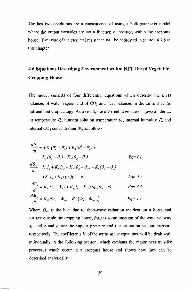
The type o f glazing material used influences the thermal properties o f the cropping house Glass which is the traditional glazing material, has largely been supplanted by other newer and cheaper materials such as polycarbonates which are good insulators There is a trade off here, because the optical transmission coefficients of polycarbonates tend to be lower than that oi glass 1 he optical transmission coefficients o f the plastics also degrade with time and they attract dust particles (Me Dowell 1994) It is advantageous to use the more robust plastics in a unit such as the one used in this work

I nnsmission cocflicient & Uvalue [W/sqm]

7 6 6

6

5

4

3

2

1 0 65

0 l

H I nnsmisswn Cocflicicnt I 1U l ictor

Single G h/cd G hss (Roylc

1984)

Double Ghzcd Glass (Roylc 1984)

4 54 1

0 63 0 76

Iy * * j a V

Single I aycrcd

Polylhuie (O I hhcrty

3 2

0 55

I win Will Polycnrbonatc (Me Dowell

1994)

Figure 2 1 Thermal and Optical Pioperties o f Vat tous Cover Mat et ials

8

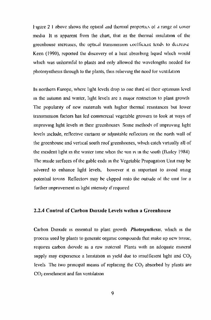
l*igure 2 I above shows the optical and thermal properties ol a range ol cover media It is apparent from the chart, that as the thermal insulation o f the greenhouse increases, the optical transmission coelllcicnt lends to decrease Keen (1990), reported the discovery of a heat absoibing liquid which would which was unharmful to plants and only allowed the wavelengths needed for photosynthesis through to the plants, thus relieving the need lor ventilation

In northern Europe, where light levels drop to one third oi their optimum level in the autumn and winter, light levels are a major restriction to plant growth The popularity o f new materials with higher thermal resistances but lower transmission factors has led commercial vegetable growers to look at ways o f improving light levels in their greenhouses Some methods o f improving light levels include, reflective curtains or adjustable reflectors on the north wall o f the greenhouse and vertical south roof greenhouses, which catch virtually all o f the incident light in the winter time when the sun is in the south (Bailey 1984) The inside surfaces o f the gable ends in the Vegetable Propagation Unit may be silvered to enhance light levels, however it is important to avoid using potential toxins Reflectors may be clipped onto the outside of the unit lor a further improvement in light intensity if required

2.2.4 Control o f Carbon Dioxide Levels w ithin a G reenhouse

Carbon Dioxide is essential to plant growth P h o t o s y n t h e s i s , which is the process used by plants to generate organic compounds that make up new tissue, requires carbon dioxide as a raw material Plants with an adequate mineral supply may experience a limitation in yield due to insufficient light and C 0 2 levels The two principal means o f replacing the C 0 2 absorbed by plants are C 0 2 enrichment and fan ventilation

9

2 2.4 1 C 0 2 Enrichment

CO 2 levels in a greenhouse can be increased by employing C 0 2 e n r i c h m e n t

The idea o f enrichment as the name suggests is to supply additional C 0 2 to the plants Commercial growers use C 0 2 enrichment during the winter and early spring Enrichment brings the added advantage that valuable heat is not lost through convection to the external environment A concentration l i f t (where a lift is understood to be an increase in a measured quantity from outside levels to those measured inside), irom the ambient 340 vpm to 1000 vpm is common (Hand 1986a) As temperatures rise in late spring, it becomes necessary to ventilate, to limit the temperature lift in the enclosure due to solar heat gain It then becomes impractical to use enrichment, since the C 0 2 is immediately lost by ventilation

Some growers use enrichment to keep concentration at the ambient level o f 340 vpm This method is called p a r t i a l e n r i c h m e n t The advantage o f this scheme is that no C 0 2 is lost to the external environment since no concentration gradient exists

10

2 2 4 2 The Drawbacks of C 02 Enrichment

Enrichment is not without its drawbacks however Burning materials such as Natural Gas or Butane to release C 0 2 will also generate trace quantities o f other gases, such as nitrogen, which may affect the growth of the crop (Hand 1986b) Compost also releases a quantity o f CO2 during fermentation This enhances the growth o f plants in traditional greenhouses (Meath 1993), but is not feasible in a hydroponic system Yeast also releases CO 2, but only in relatively small quantities and the life span o f an active yeast plant is typically 4-5 days (Yeast products 1994) For large scale installations, bottled CO2 is too expensive to use, but in miniature houses like the one under consideration here, it could be used effectively The main restriction on bottled C 0 2 is availability With only one major supplier o f industrial grade C 0 2 in the country it is difficult to guarantee a steady supply

The cost o f CO 2 sensors is another drawback A typical commercial automatic C 0 2 sensor can cost anything between £500 and £3000 Though C 0 2 test kits are available for about £200 (Hand 1986b) For a small unit this cost is prohibitive In chapter 5, a possible solution to this problem will be suggested

2 2 4 2 Ventilation to Prevent C 0 2 Depletion in the Cropping House

It is important that the C 0 2 levels do not drop far below ambient, as this decreases the photosynthetic rate o f the plants Hand (1986a) found that at an air temperature o f 20°C, the photosynthctic rate decreased by 9% in bright light and 6% in dull light for a 10% drop in C 0 2 concentration below the ambient 340 vpm Hand, and Tarm Electric (1973 after Gaastra 1959) note that photosynthesis almost ceases when adequate light is available and C 0 2 concentration drops below 50 vpm This o f course is undesirable and ambient

II

levels are required where possible So in the absence o f C 0 2 enrichment, it becomes necessary to ventilate to ensure that CO 2 levels are adequate particularly during periods o f bright sunshine when the plants are photosynthesising, but also at night when the plants are respiring and there is a build-up o f CO 2 in the cropping house

2.3 Control o f the Rhizosphere

The term rhizosphere can be used to describe the vicinity o f the root In conventional greenhouses, this area is not directly controlled However in hydroponics-based cropping systems, there is no soil to protect the roots from extremes o f temperature or to protect against excessively rich and potentially toxic mineral supplies

2.3.1 The N utrient Film Technique

H y d r o p o n i c s is a word which is used to describe methods o f growing plants in soil-free nutrient solutions Artificial materials such as rockwool, sand or sawdust may replace soil to support the root systems o f the plants W oodward grew plants in a soil-less culture in 1699 The first true hydroponics systems were developed independently for laboratory use by Sachs and Knapp in 1860 I he first iull-scale commercial application of hydroponics was reported by Gericke in 1940 He also in passing, coined the word hydroponics (Jenson and Collins 1983)

The N u t n e n t F i l m T e c h n i q u e ( N F T ) , which will be considered in this work and is illustrated in figure 2 2, is called a l i q u i d h y d r o p o n i c system since it requires no root support medium The Nutrient Film Technique was developed

12

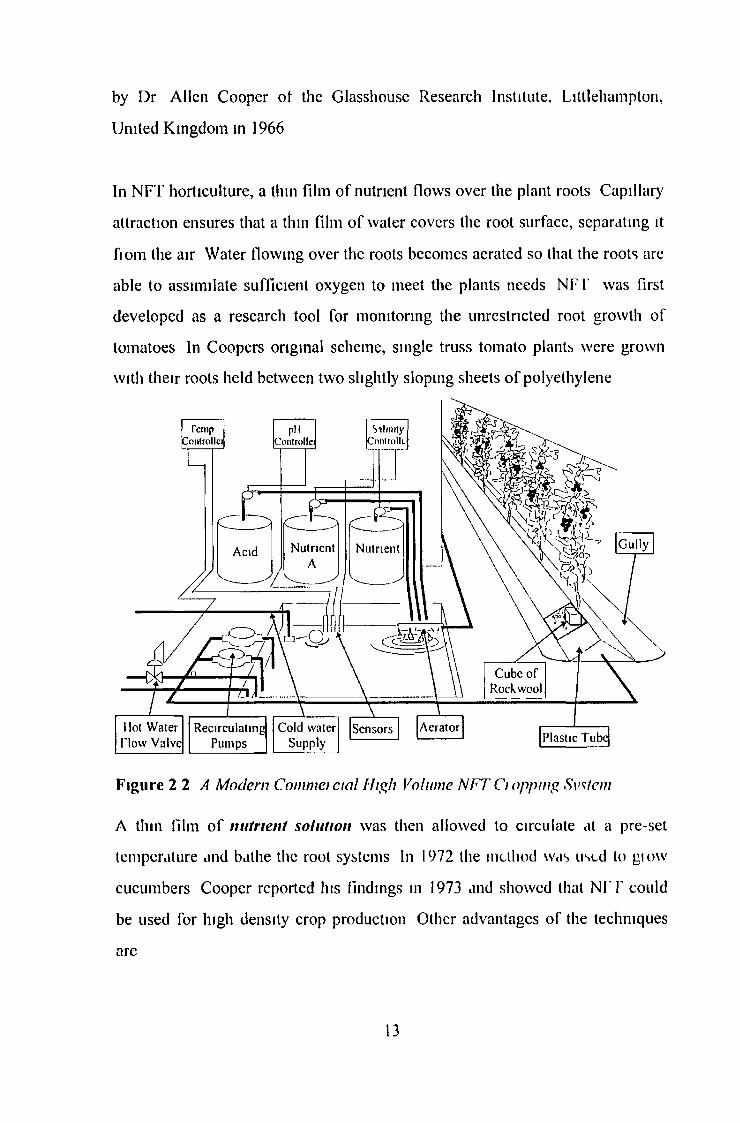
by Dr Allen Cooper of the Glasshouse Research Institute, Littlehampton, United Kingdom in 1966

In NFT horticulture, a thin film o f nutrient flows over the plant roots Capillary attraction ensures that a thin film o f water covers the root surface, separating it ftom the air W ater flowing over the roots becomes aerated so that the roots are able to assimilate sufficient oxygen to meet the plants needs NFT was first developed as a research tool for monitoring the unrestricted root growth of tomatoes In Coopers original scheme, single truss tomato plants were grown with their roots held between two slightly sloping sheets o f polyethylene

Figure 2 2 A M o d e r n C o m m e t c m l H i g h V o lu m e N F T C i o p p m g S y s t e m

A thin film o f n u t r i e n t s o l u t i o n was then allowed to circulate at a pre-set temperature and bathe the root systems In 1972 the method was used to glow cucumbers Cooper reported his findings in 1973 and showed that NFT could be used for high density crop production Other advantages o f the techniques are

13

• Economic use o f plant nutrients• Crop production where no soil exists, eliminating need lor soil sterilisation• Conservation o f soil ecosystems• Isolation o f crop from soil (to reduce risk o f disease, salinity problems)• Control o f conditions in rhizosphcre to optimise mineral ion uptake• Rapid crop turnover• Minimal exposure o f rhizosphere to pathogens such as wilt, fungi and

nematodes

Between 1973 and 1985 the technique was adopted widely by horticulturists However due to the rising costs o f oil, prohibitive initial capital costs and the level o f expertise required to use the technology effectively, the original method ceased to be cost effective Modified N IT techniques were then developed Teagasc’s Kinsealy Research Station conducted extensive trials on N H m the mid 1980’s They presently prefer an aggregate technique in which they allow nutrient to propagate through enclosed rockwool R o c k w o o l is a mesh o f benevolent recycled mineral threads through which plant roots arc permitted to spread The fine mesh causes capillary action to take place, thus permitting water to reach roots (Maher 1993) I here has been much controversy however, as to which strategy produces the best results (Cooper 1983), and NFT is still used by commercial growers in noith County Dublin (Fisher 1994)

2.3 2 The W ater Supply in an NFT System

A plentiful and regular supply o f aerated water is essential lor any hydroponics system A typical tomato plant in a protected environment will consume about 1 3 litres o f water on a bright summer day Winsor (1980), discovered that tomatoes lost water at 15 ml/hr/plant at night, but losses rose to 135 ml/hr/plant on a cloudless summer day Adams (1980) noted that the water uptake for

14

cucumbers is twice that for tomatoes and varies linearly with incident radiation. Modern commercial systems generally contain sufficient water so that the nutrient is replaced once a day (Hurd and Graves 1981). The amount o f Oxygen dissolved in the nutrient solution will also affect the flow rate. This matter will be discussed later in this chapter.

2.3.3 M ineral Requirem ents o f Plants

Different plants have different mineral requirements and so, unwanted and potentially toxic ions may build up in the solution. Even if the solution is not toxic, the unwanted ions may prevent osmosis o f the desirable nutrients into the root. These problems are o f major concern for large volume growers. Consequently, conductivity and pH control systems are used to monitor and control the salinity and acidity o f the nutrient. These control systems are difficult to maintain and are often dependent on the crop type. A major disadvantage o f NFT is that since there is no solid material enclosing the roots, there is nothing to act as a buffer against toxicity in the nutrient supply. It is desirable to keep pH levels between pH 5.5 and pH 6.5, where optimum ion uptake occurs (Graves 1985).

The quantity o f nutrient in a hydroponic solution does not have to be as high as in conventional systems since the flow guarantees that the nutrient gets to the root. This is not the case in conventional systems where the root depends on diffusion for its supply o f nutrient. For lettuce, salinity o f between 1500 jiScm '1 and 1800 jxScm'1 is recommended (Burrage & Varley 1980). O f course, conductivity is only a measure o f the quantity o f salt in the nutrient, and is virtually unaffected by the amount o f trace elements present. It also depends on the type o f nutrient used as some solutions contain chclated compounds which have lower than average conductivities for higher concentrations.

15

Nutricrop which is the commercial nutrient used in this work, contains chelated compounds The suppliers recommend a conductivity o f 200-600 |iScm 1 From tests conducted on plants, a conductivity ol 400 j.iScm 1 was found to produce satisfactory results

2.3.4 The Effects o f Root Zone W arm ing

Root temperature is known to be a critical determinant o f the productivity of hydroponic systems Root zone warming is known to increase the rate ol fruit production It has been shown that control o f the root temperature can shorten or lengthen growth cycle ot tomatoes (Hurd and Graves 1984),(M aher ct al 1993) After the energy crisis in the 1970’s, growers began to research using reduced night-time air temperatures (Jenson and Collins 1983) W henever air temperatures below 12°C are used for NFT systems, it is necessary to keep solution temperatures within the range 13°C - 15°C, to prevent reduced uptake of nutrients (Moorby and Graves 1980) Nulncnt in an unhealed NT I system may become cold enough to check root growth severely Evaporative cooling may cause the nutrient temperature to drop below the air temperature (Graves 1985) NFT is readily adaptable to root zone warming

Solution temperature is relatively inexpensive and simple to control accurately, whereas a control system for soil temperature would be expensive to install and operate An acceptable optimal range for nutrient temperature in full sunlight is 25°C with an acceptable optimal value o f |ust over 20°C (Grower Books 1982) It is known that fruit picking in plants grown in an NTT solution, is accompanied by a period ol root death It has been found that root temperatures of 25°C around picking time in an early tomato crop can increase the yield o f

1 6

fruit, but will not shorten the delay caused by low air temperatures (Hurd and Graves 1984).

2.3.5 The Need for an Adequate Oxygen Supply to Roots

Roots need a constant supply o f oxygen. Since oxygen is virtually insoluble in water, it is undesirable to have the roots more than partially submerged in nutrient. A mature tomato plant requires 20 ml o f oxygen per hour (Graves 1985). NFT resolves this problem by allowing water and air to mix freely, thus guaranteeing an abundant supply o f oxygen to the root. Increases in water temperature decrease the saturation concentration o f oxygen in the water. At 25°C the saturation concentration is 8.5 ppm (Jackson 1980). This means that if the root is submerged in the nutrient that the water would have to be passing the root at a rate o f 0.65 Is'1. If the roots are only partially submerged however, oxygen may be absorbed directly from the air so this value is an upper limit on the flow rate.

2.3.6 Other Considerations

Care must be taken when choosing materials for an NFT system. Wavin Plastics warn against the use o f galvanised fittings which can lead to a build-up o f unwanted substances in the solution to toxic levels. Some plastics however, are also dangerous to plants. Among those which have been found to have detrimental effects are ABS and Plasticised PVC. Where it is necessary to use a metal, it is preferable to use stainless steel fittings. Though stainless steel is difficult to shape and expensive to buy, it is relatively inert. Another danger to plants comes from stabilisers and pigments for otherwise safe plastic fittings which may also contain toxins. The catchment tank for small scale systems is

17

oiten constructed ot fibreglass, since this is generally sale to use but sub|ect to the same constraint (Graves 1985) It is prudent therefore to request ‘food handling grade m aterials’ when ordering materials which may come into direct or indirect contact with the nutrient (Grower Books 1982)

2.4 Review o f Limits and Optimum Values of Param eters in an NFT Control System

This chapter has summarised currently available information regarding lactors determining optimal productivity in NFT systems Desirable ranges and optimal values o f physical parameters which affect plant growth derived from the preceding discussion are tabulated below

Table 2 1 Limits foi Controlled Pat ametei s in an Envu onmental Conti olSystem for NFT

Parameter DAY NIGHTRelative Humidity < 85% Same

Nutrient Temperature 20 - 26°C 24°C Optimum

13- 15°C

Nutrient Flow Rate Past Roots

0 125 lmin 1 Same

C 0 2 Concentration Near 340vpm SameNut Solution Conductivity

Using Chelated Compounds

200 - 600 jiScm 1 400^iScm"1 Optimum

Same

Air Temperature 15 - 22°C 5 - 15°CNutrient Solution pH pH5 5 - pi 16 5 Same

lab ie 2 1 can be shoitencd to include only those quantities which will be dealt with in this study The night-time nutrient solution temperature range has been relaxed to allow for the power limitations o f the water heaters Digital control o f conductivity and pH o f the nutrient solution will be left for later work

1 8

Table 2 2 Limits and Prefer)ed Values fo / Controlled Parameters in the Miniature Ci opping House

Parameter DAY N1G11TAir Temperature 15 - 22()C 5 - I5°C

Relative Humidity < 85% SameCO 2 Concentration Near 340vpm Same

Nutrient Temperature 20 - 26°C 24°C Optimum

8 - 15°C

Nutrient Flow Rate Past Roots 0 125 Imin 1 Same

The values shown in table 2 2 will now form the basis for a control strategy which will attempt to keep these parameters within these ranges or at the appropnate values It is apparent from table 2 2 above, that some form o f rule- based approach would be suitable for transforming the above set o f constraints into a control strategy The next chapter will describe one such a rule-based control strategy which may be used to control the environment inside the cropping house

19

Chapter 3: Fuzzy Logic Control

3.1 An Introduction to Fuzzy Logic Control

Agucultural scicncc like medicine, is not always an exact sciencc As can be seen Irom chapter 2, many ol the control leqununcnts lor an Nf 1 system are not easily transierred into a classical control strategy Growers Irequently tend to use their senses and expert judgement rather than instiumentation when making decisions which may affect the crops As a result, it is difficult to obtain optimum figures for humidity, air temperature, nutrient temperature, and C 0 2 concentration for a particular cultivar In addition, these requirements may often contradict each other, may depend on stage o f growth and will almost certainly be expressed in a linguistic way

Since the control strategy for regulating the environment in an NTT systemtrelies on rules, it is necessary to use some form of rule-based control One foim

o f rule-based control is called fuzzy logic control The following discussion examines the operation o f a fuzzy logic engine, which is an all-purpose fuzzy logic system with an emphasis on its use as a controller

Figure 3.1 Elements o f a Fuzzy Logic Conti oiler

Figure 3 I shows the three main processes at work in a fuzzy logic controller Fuzzification is a means o f converting a measured value into its equivalent fuzzy representation Fuzzy inferencing allows this information to be combined

2 0

with fuzzy rules to form a conclusion which will still be in the fuzzy domain Finally, defuzzification as the name suggests, is the process o f converting the output o f the inferencing mechanism back into a non-iuzzy output value which can then be applied to the plant The following sections briefly describe the operation o f a fuzzy logic controller

3.2 Introduction to Fuzzy Logic

Fuzzy logic was first conceived as an extension o f muiti-vaiued logic, by Lotfi Zadeh o f the University o f California at Berkeley in 1962 Zadeh describes fuzzy logic as a translation mechanism which translates a human solution to a problem, into the language o f fuzzy rules For instance a driver o f a car relies on judgement to decide if the car in front is too close and responds by adjusting the accelerator The text o f an appropriate fuzzy rule for this situation might be IF THE CAR IN FRONT IS TOO CLOSE, THEN SLOW DOWN The point at which the driver eases back on the accelerator is not clearly defined since the transition from a safe distance between cars, to an unacceptable one is gradual This gradual change in the suitability o f a term such as TOO CLOSE to describe a situation, is quite commonly encountered and can be readily described using the idea o f partial set membership, which is central to fuzzy logic

The idea o f ambiguity is inherent m the way in which we describe the world around us Information transferred using everyday language may include ideas such as the adjectives “VERY’' and “SLIGHTLY" which are not easily described using existing mathematics Fuzzy logic also has features which capture this additional information and it is therefore well suited for storing linguistic knowledge

2 1

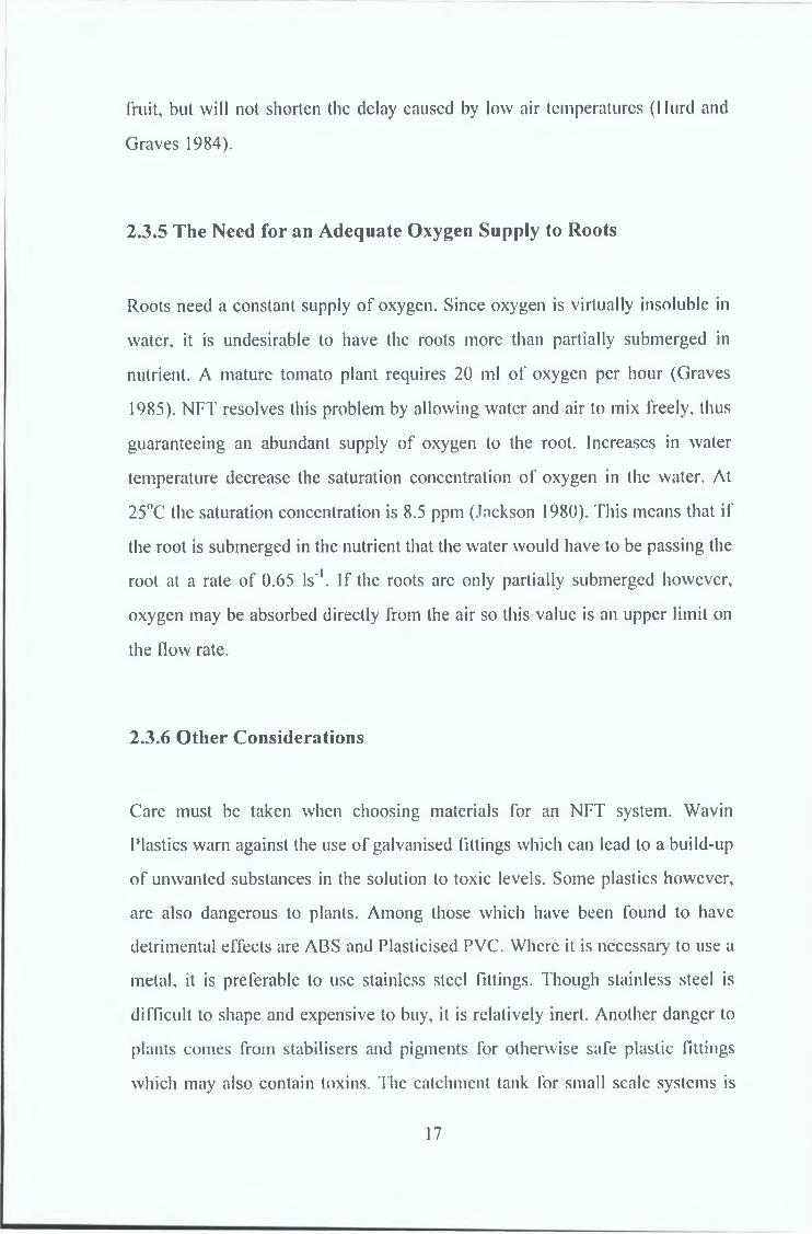
The principal difference between crisp logic and luzzy logic is that while crisp logic only allows for membership or non-membership oi a set, fuzzy logic permits an element to be a partial member o f a set In a crisp logic system for instance, one might judge the temperature o f water in a shower to be a member o f the set HOT and not a member o f the set COLD This does not allow lor uncertainty in the definition o f the terms HOT and COI D Using fu //y logic however, we might say that shower temperature is HO Y to degree 0 7 and COLD to degree 0 3 This allows the sets HOT and COLD to overlap The numbers 0 7 and 0 3 are an indication o f the extent to which a temperature measurement belongs to each set They are known as g r a d e o f m e m b e r s h i p

v a l u e s and are usually signified by the symbol \x A function which is used to describe the degree o f membership for any member o f a fuzzy set is called a m e m b e r s h i p f u n c t i o n Functions o f this type are shown in figure 3 2 below

Figure 3 2 Fuzzification o f a C; isp Measurement Using Triangula/ Sets

3,3 Fuzzification

Figure 3 2 shows the membership functions o f three f u z z y s e t s , which are being used to describe a temperature I he words used to describe each set are called

f u z z y l a b e l s The space on which the sets exist is called a u n i v e r s e o f d i s c o u r s e

U , which in this case lies between 0°C and 100°C Notice that the c r i s p

m e a s u r e m e n t o f 85°C has a non-zero membership o f the sets H ot and W arm

2 2

The sets shown above may be represented by a set of lin ear sp lin es L{ u, a, b, c) as follows -

L{u, a,b,c)

0(u - a ) / { b - a ) (u - c ) / { h - t )

0

foi u < a

for a < u < b

for b < u < c

foi u > c

E qn 3 /

where a ,b and care any three consecutive points on U as shown above and u is the crisp measured input which is also on U

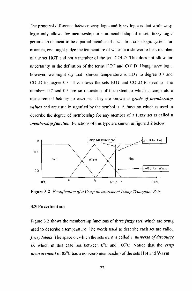
Membership functions do not necessarily have to be piecewise linear Indeed, bell shape functions favoured by statisticians are frequently used when precise definitions o f fuzzy sets are required The S -functton s(it, a, b ,c ) approximates these functions using quadratic approximations as follows

s {u,a,b,c)'

0 foi if < a

2[{u - a)/{c - a)]2 fat a < u < b

/-2[(i/-c)/(c-a)]2 foi b < u < c

0 fot u > c

Eqn. 3 2

Notice that the membership values for the S-function, shown in figure 3 3, are less likely to be near the ambiguous value of 0 5 than those generated by the linear splines for the same crisp input The obvious shortcoming of this type of membership function is that it requires moie computation S-lunctions are usetul for applications such as medical diagnosis where a high degree of precision is required and there arc relatively lew time constraints

23

0°C a b 85°C c IOO°CFigure 3 3 Fuzzification Using S-function Mem bet ship Functions

For this work however, it will be sufficient to define sets using linear splines A fuzzy set may be represented as a set of ordered pairs of an element u and its associated grade of membership which may be determined by evaluating the membership function at that point

F = [(i/,|i(//) )|wct/} Eqn 3 3

Where U is the universe of discourse

Thus the first stage of the fuzzy logic controller, called fuzzification, takes each crisp measurement it and assigns a value which correspond to its degree of membership of each of the fuzzy sets available to it across the universe of discourse The crisp measurements arc now said to be f u n i f ie d

3.4 Inferencing

The inferencing stage extends the linguistic description so that the fuzzified measurements suggest lu//y “icsults" I his is done by Juzzy in feren cin g I u //y inleicnung is a method which uses data liom one universe ol discourse to loim conclusions in another (Dexter 1992) We shall see that the inference mechanism uses so called fu z zy operators to implement the mathematical

24

equivalent of statements such as IF SHOWER IS HOT THEN MAKE IEMP VERY LOW These statements are called rides The First part of the rule, called the iuIc p rem ise is composed oi anteceden t sets 1 he sccond part ol the lule, the part after the THEN, is called the con sequ en t A collection of fuzzy rules is called a fu z z y ru lebase The example below which shows part oi a fuzzy rulebase, illustrates these terms

___________________________ Rule__________________________________________________ Premise___________________ Antecedent ____ Antecedent Consequent_IF SPEED IS HIGH AND DISTANCE IS SHORT TIIEN BRAKE IIARD IF SPEED IS MEDIUM AND DISTANCE IS SHORT THEN BRAKE MEDIUM IF SPEED IS LOW AND DISTANCE IS SHORT THEN BRAKE OrF

As can be seen above, the phrases IF SPEED IS HIGH and AND DISTANCE IS SHORT are antecedents in the First rule When they are combined they form the phrase IF SPEED IS HIGH AND DISTANCE IS SHORT This longer phrase is the premise of the rule Finally the consequent of the first rule is THEN BRAKE HARD

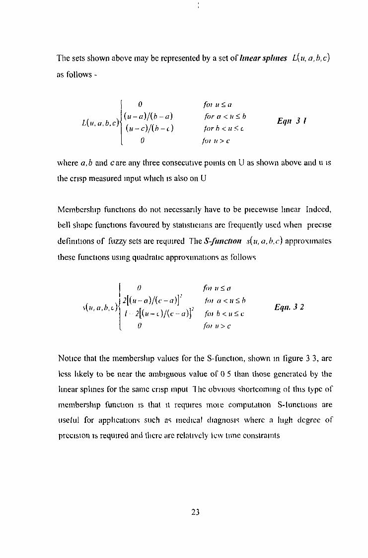
The tuzzy operator referred to above is called a t-nornt T-norms map the grade of membership of each set on the input universes o f discourse to a D egree o f

fu lf ilm e n t of a fuzzy rule on the output universe The degree of fulfilment of a rule is a measure o f how appropriate it is to use that rule to respond to the crisp measurement Examples of t-norms are the p rod u ct function and the nun function The degree of fulfilment of the fuzzy rules are said to qualify the consequent sets The usual effect of such operators is that the shape of the set is changed Qualification using the product (scaling) and the min (clipping) t- norms is shown below in figure 3 4

25

The m axim u m values of the qualified consequents form a single fuzzy set which is called a fu z zy com position The fuzzy compositions resulting from scaling and clipping are shown at the bottom of figure 3 4

Rule I

Min and Product InferencmgTuzry Output Using

Mtn Inlcrcncing

\ ui/y Ouiptll Uülinr Prod Infcrcncmg

Fig 3 4 Min and Product Inferencmg

Figure 3 5 below shows a two dimensional plot of the output resulting from a range of non-luzzy inputs to a controller It shows the conti lbulion of the rule to a range o f control efforts

IF INPUT 1 IS SET1 AND INPUT2 IS SET1 THEN OUTPUT IS +0 5

In this case the premise is a two dimensional fuzzy set The two dimensional membership function of this set is shown in figure 3 5 (Degree of Fulfilment of Rule) This membership function may be considered to be a plot of the degree of fulfilment of the rule for every combination of input values IP1 and IP2 I igure 3 5 (Deiuzzilled Outputs) is composed ol the weighted degrees ol

26

fulfilment of four such rules For the rule shown above, the weighting is +0 5 Figure 3 5 (Defuzzified Outputs) is called a fuzzy control surface A control surface will exactly mimic the fuzzy logic controller However, if a lookup table or a set of splines (Hams 1993), is used to deliver the required action, the linguistic knowledge contained in the fuzzy rule-base is lost

Input 1 Set 1

Input 2 Set 1

D egree of Fulfilment of Rule

Defuzzified Outputs

Figure 3 5 Generation o f a Fuzzy Control Surface Using Product Infer encing

27

3.5 Defuzzification

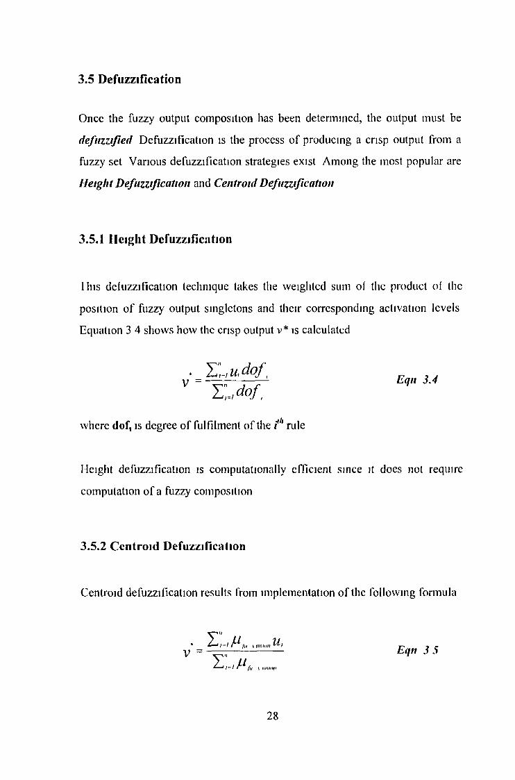
Once the fuzzy output composition has been determined, the output must be defu zzified Defuzzification is the process of producing a crisp output from a fuzzy set Various defuzzification strategies exist Among the most popular are H eigh t D efuzzification and C entro id D efuzzification

3.5.1 H eight Defuzzification

1 his defuzzification technique takes the weighted sum of the product of the position of fuzzy output singletons and their corresponding activation levels Equation 3 4 shows how the crisp output v* is calculated

• T,.,u,dof, r , ,_ — i------------ - Eqn 3 .4Z - M ,

where dof, is degree of fulfilment of the f h rule

Height defuzzification is computationally efficient since it does not require computation of a fuzzy composition

3.5.2 Centroid Defuzzification

Centroid defuzzification results from implementation of the following formula

* = l ^ fu I unnnt -V = E qn 3 51-1 fu i union

28

Where JUfuzzyunion is a function of u resulting from taking the su prem u m o f allthe qualified fuzzy sets Supremum is a word used to describe a function which will select the greater of two grades of membership if given a choice (Lyons 1993) Of the two methods, centroid defuzzification which is sometimes referred to as centre o f area defuzzification, is more computationally intensive but produces a smoother control action than height defuzzification

3.6 The Reason for Using Fuzzy Logic m Environm ental Control

A commonly voiced objection to fuzzy logic controllers is that they are primarily of use where a model of the plant does not exist and otherwise, more conventional control strategies should be used Conventional non-linear controllers may be created by using control surfaces or lookup tables which will determine the output of the controller for different input values Unfortunately these methods require the designer to be familiar with control system theory They may also be quite time consuming to design PID controllers are easier to design and are used extensively in industry, but PID controllers are not always suitable for controlling non-hnear systems like the one discussed here In contrast, fuzzy logic controllers may be used to quickly translate heuristic expert knowledge such as that given in table 2 1 into a control strategy Modern commercial fuzzy logic development packages are quite user-friendly and the level of understanding of the system necessary to design a fuzzy controller is moderate

Simple deterministic models of environmental systems like the one introduced in the next chapter are rarely extremely accurate So in effect, even though the model will mimic the system, and the user may change the parameters it will only give an indication of how the real system will behave The low-pass nature ot the set shapes in a fuzzy controller peimits it to cope well with inaccuracies

29

between model and system and a well designed luzzy controller may continue controlling even in the event of sensor failure It is this feature which has prompted its use 111 backup control systems lor nuclear reactors (Bernard Lt A1 1985)

3.7 Fuzzy Logic and Expert Control

The first application of fuzzy logic control was for the control ol an experimental steam engine (Mamdam and Assilian 1975) Since then, fuzzy logic has been applied to a large variety of control problems Among the more unusual are flight control of a model helicopter (Schwartz and Klir 1992), and intelligent washing machines and rice makers ( Mamdam 1992)

Fuzzy logic control appears to date, to have been used chiefly in situations wheie little is known about the dynamics of the plant Although Mamdam (1993) suggests that it is this conservative attitude among Europeans which has allowed Japanese researchers to become world leaders in fuzzy logic research

In recent years, fuzzy logic has been used increasingly for environmental control (MacConnell et al 1993), (Tobi and Hanafasu 1991) The lack of understanding of the physical processes occurring in such systems makes it difficult to control them using standard control techniques Earlier in this chapter, it was mentioned that climate control systems for cropping houses have the additional difficulty that the optimum climate for plant growth may not be known It is not surprising therefore that fuzzy logic control should be applied to this type o f problem

As we shall see later, the most dilficult aspect of controlling the unit is the control of humidity/air tcmpcrature/C02 concentration It is to this aspect ol the

30

control problem that fuzzy logic control will be applied Since the controller will be performing the same task as a grower in deciding what the values o f the above parameters are appropriate lor a given set o( external conditions, the control may be termed “E xpert C on tro l” From the preceding explanation oi luzzy logic, it becomes apparent that iuzzy rulebases may be easily ioimed from the relatively vague expert knowledge ol the grower The more linear processes such as nutrient temperature and conductivity will be controlled using standard control techniques

The rule-base for the expert fuzzy controller will be chosen using a combination of knowledge gained by observation from table 2 1 and from consulting with experts This issue will be further addressed in chapter 5

3.8 Further Reading

Over 9000 papers, books and reports have been published on fuzzy logic since 1965 (Harris et al 1993) Cox (1992) Schwartz and Klir (1992) and Self (1990) are three articles which give a simple introduction for those who have no experience o f the technique The Motorola Fuzzy Logic Tutorial is a particularly useful introduction to the topic and is available for a token fee from Motorola’s Document Supply Centre in the UK (Lee 1990a, 1990b) has produced a concise overview of fuzzy logic for those who wish to delve deeper into the topic Arguably the most readable work on the links between fuzzy logic and neural networks is Harris (1993)

31

Chapter 4: Model Of Miniature Cropping House

4.1 Introduction

The purpose of a greenhouse is to provide an energy efficient and favourable growing environment for plants The former usually results in large and expensive-to-run commercial greenhouses The considerable cost of using a full-scale greenhouse to test a particular control strategy, led engineers and environmental physicists to develop mathematical models that mimic the behaviour of such systems These models can be used to aid the understanding of the behaviour o f the greenhouse under diflerent environmental conditions Dent and Blackie (1979) give the following additional uses of models of agricultural systems

• They are a means by which experimental studies may be guided• Results of such work can be easily accumulated and assessed• They are a platform to guide the development of new systems

The complexity of a model should reflect the purpose for which it is designed l o r example, a model ot the dynamics ol an aircrait lor a flight simulator would need to be more accurate and hence more complex, than a similar model for use in a computer game simulation

Due to the degree of non-linearity of the parameters in models which describe environmental systems, as well as the amount of interaction, the creation of environmental models may be problematic Later, it will be seen that in the model described here there is interaction between the inside air temperature, nutrient solution tcmpciature and inside humidity, all of which are output

32

variables in the model llie chiel sources ol non-linuiritits aie the equations describing humidity, C 02 concentration and the fan characteristic

4 2 Types o f M athem atical M odels used For Describing Environm ental System s

Mathematical models of environmental systems such as greenhouses can be divided into three main categories,

• D eterm in istic M odels may be developed from elements of environmental physics

• H eu ristic M odels depend on expert knowledge of the cropping house and may be accumulated in rules that will govern the response of the model to external stimuli, or may simply take the form of an empirical charactenstic equation

• Iden tified M odels use identification algorithms to determine the relative significance of cach parameter in a model lather than relying on physical principles

Models may also be dynamic or static A sta tic model predicts the final value that each output variable will take, when variables or other parameters in the model are changed A dyn am ic model also takes account of the storage capacities of some variables in the model For this reason, the dynamic model can be used to study the behaviour of a system, as external conditions change over time

A deterministic greenhouse spatial model can be zero dimensional, one- dimensional or three dimensional Zero Dimensional or bulk p ara m eter models assume that conditions in each clement ol the model are homogeneous O ne

33

d im en sion a l m odels assume that conditions in the greenhouse will only change as a function of height Three d im en sion al m odels on the other hand, also allow for changes in parameters at different positions m a horizontal plane, in addition to changes due to height

The non-linearities and interaction effects mentioned at the end ol section 4 1 affect deterministic and heuristic models in particular, since the nonl-inearities may be difficult to describe using standard physics or may not be well understood in a linguistic sense These difficulties may be overcome in some cases, by replacing the deterministic/heuristic models with identified models, which are known to be good at mimicking the system for which they are created Identified models however are chiefly suited to modelling systems whose dynamics do not change over time In addition, they are generally only accurate for mimicking conditions close to those under which they were identified Consequently, most models involve a combination of some or all of the above three approaches For this work, the model will be predominantly deterministic and based on plant physics There will however, be elements of heuristic and identified modelling

4.3 Controlled V ariables in a Com m ercial H ydroponics-Based Cropping System

The main controlled variables in a conventional greenhouse are as follows

• Air temperature• Humidity• C 0 2 concentration

34

A hydroponics system requires the control of some additional quantities These are

• Nutrient temperature• Nutrient concentration• pH of nutrient

This chapter will follow the development of a mostly deterministic model that will predict the behaviour of the first four of these parameters namely, air temperature, humidity, C 02 concentration and nutrient temperature within the miniature cropping house

Seginer and Levav (1971), have identified the need for researchers to develop models which include only p rim ary boundary con dition s Primary boundary conditions are environmental parameters afletting conditions mside the greenhouse which are easy to measure and are unaffected by the existence of the greenhouse (Kindelan 1980) An example of a primary boundary condition is the intensity of light incident on the outside surfaces of the cropping house A secon dary bou ndary condition is a parameter which is affected by the existence of the cropping house The intensity of light incident on the crop canopy inside the cropping house, is a secondary boundary condition

Using secondary boundary conditions makes the cropping house model less useful, since it then requires information about conditions inside the cropping house A model using only primary boundary conditions, can operate using only meteorological data from the intended location of the cropping house The deterministic model introduced in this work will thcreiore use primary boundary conditions only

35

Many control strategies require the designer to provide a mathematical model of the plant, before the controller can be implemented At least some knowledge of the plant is required in almost all cases For example, before tuning a PID controller for optimum periormance in a particular application, it is usual to perform some form of system identification such as, using a process reaction curve to determine the steady state gain and the time constant of the system

Fuzzy logic control requires trials to be conducted belore the controller designer will be familiar enough with the controlled system to create a fuzzy rule-base and fuzzy sets This process can be made easier if a model exists on which the controller may be tested initially and then fine-tuned on the real system

The first part o f this chapter will consider the development of the model This will be followed by qualitative and quantitative assessments ol its periormance

4.4 D evelopm ent o f the Determ inistic M odel o f an NFT Cropping SystemInitial work on dynamic deterministic models ior greenhouses was done by Businger (1963) who developed a steady state model of the environment inside a greenhouse This was iollowed by probably the most referenced and comprehensive work on deterministic models by Seginer and Levav (1971) They developed a static one dimensional static model of a greenhouse similar to that o f Businger and extended it to three dimensions Work by Udink len Cate (1983) on a bulk parameter dynamic deterministic greenhouse model was extended and adapted to model a mushroom growing tunnel by Hayes (1991), whose equations described the heat and mass fluxes occurring between the internal air, the external environment and the crop

36

Meath (1993) further developed Hayes’ model with particular emphasis on the equations describing humidity in the mushroom house Mushroom houses have concrete floors and concrete has a large thermal capacity Consequently, the temperature of the floor changes very slowly relative to the air temperature Thus Meath did not include an equation describing the floor temperature dynamics

Hydroponic cropping systems include a relatively large quantity of a solution of water and nutrient concentrate The thermal capacity o f the volume of water in the hydroponics based vegetable cropping house, is relatively low compared to that of a concrete floor and consequently the dynamics are substantially faster This means that they are much closer in reaction time to the dynamics o f air temperature and thus cannot be neglected Since the temperature of the nutrient- water mixture is to be controlled, it is necessary to extend the Meath and Hayes models to include water temperature

Figure 4.1: Block Diagt am o f Model o f Mimatw e Ci opping House

37

Figure 4 1 above shows the inputs to the model and the interaction between equations The model accepts incident solar radiation, external air temperature, external humidity and outside CO2 concentration as uncontrolled inputs Water temperature and internal air temperature, humidity and C 02 concentration are alfected by the water heater and fan speed respectively, as indicated Fig 4 2 shows how these parameters are to be measured and controlled in the real system

4.5 Assum ptions for Determ inistic M odel o f M iniature Cropping House.Before showing the set of equations which define the model, it is necessary to state the assumptions under which the model was constructed These are listed below

• Solar radiation which has been transmitted through the cover, reaches only the floor and/or the plant canopy and not other parts of the structure and does not directly heat the air inside the enclosure

• All surfaces radiate long wave radiation like black-bodies• Short-wave radiation absorbed by the floor, is re-emitted as long-wave

radiation in the form of heat• The significant dynamic factor in the water temperature balance, is the

thermal capacity of the tanks and not that of the trays• The resistance of the stomata in the plants to heat and moisture transfer, is a

function of ventilation rate only• The nutrient solution temperature is uniform throughout the unit• The air within the cropping house is perfectly mixed

38

I he last two conditions are a consequence of using a bulk-parameter model where the output variables are not a function of position within the cropping house The issue of the stomatal resistance will be addressed in section 4 7 8 in this chapter

4 6 Equations Describing Environm ent within NFT-Based Vegetable C ropping H ouse

The model consists of four differential equations which describe the mass balances o f water vapour and of C 02 and heat balances in the air and at the nutrient and crop canopy As a result, the differential equations govern internal air temperature 0a, nutrient solution temperature internal humidity r a and internal C 02 concentration cPm as follows

df)^ = +Kl(e:-0:)+ K2(0:-e:)+

K ,( 0 a - O J - K 4( 0 ' - 0 t) Eqn 4 1

^ - = K ,/„+ K t Q„ + K , (0t - 00 - K h (0„ - 0J+ K sIh + K J ( q J ( e 4 - e) Eqn 4 2

= K,„(Tl - r j + K ,,Ih + K ,J ( q J ( e t - e) Eqn 4 3a t i/O

dtWhere Qso is the heat due to short-wave radiation incident on a horizontal surface outside the cropping house, f ( q j is some function of the wind velocity qu and e and es are the vapour pressure and the saturation vapour pressure respectively The coefficients K t of the terms in the equations, will be dealt with individually in the following section, which explains the major heat transfer processes which occur in a cropping house and shows how they can be described analytically

39

4.7 H eat and M ass Transfer M echanism s in G lasshouses

This section introduces the individual terms describing heat and mass transfer which contribute to the heat and mass balance equations of section 4.6. Each term is described independently, is modified to suit the model and linearised where possible. The following section will show how these terms may be combined to form the four differential equations which constitute the model.

4.7.1 Short W ave Radiation

The difference in the intensity of short-wave radiation between summer and winter months is largely attributable to latitude, since this determines the angle of the solar azimuth and also the length of the day, at any particular time of the year. In Ireland and Great Britain for instance, the total energy supplied by the sun may be up to ten times less in a winter month than in a summer month. On a clear summer's day outside a greenhouse, a typical value for the flux of solar radiation would be 800 Wm'2. Dense clouds can reflect up to 70% of incoming solar radiation. Typically about 44% of total radiation is considered to be ph o tosyn th etica lly active. Of course this figure varies depending on the type of plant (Electric Council 1973). In addition, if the plant is grown in a closed space such as a greenhouse or miniature cropping house such as the one studied here, the radiation flux is attenuated by the glazing.

The co-efficient which quantifies how much light will get through the glazing of the cropping house is called the glazing transmission coefficient xc. If the incident radiation Q w is measured in Wm'2 to coincide with meteorological measurements and the total flux inside the cropping house Qs, is measured in W, then the short wave radiation flux incident on the entire plant canopy is

40

£?„ = r J l - a J A Q « , E q n .4 .5Where At is the surface area of the cover and a is the albedo of the plant, which is the fraction o f incident radiation which is reflected by the plant surface The above treatment assumes that there is no specu lar reflection , or in other words, light is incident on the glazing at an angle which is approximately normal to the surface and so is transmitted through it, rather than reflected

4.7.2 M easuring Short W ave Radiation Using a Light Sensor

In this work, the intensity of incoming solar radiation is measured using a light sensor which produces a voltage output which is a linear function of the intensity o f the incident short wave radiation At zero intensity, the device outputs 0 V, while at an intensity of 200 W in2, the output voltage saturates at approximately 4 V This can be modelled by the following light intensity to voltage characteristic

Vst- 0 02 QSIwhere Q SI is the intensity of the solar radiation in Wm' and V Si is the output voltage

4.7.3 Long W ave Radiation

Much of the short-wave radiation which falls on leaves and other surfaces is absorbed and re-emitted as less energetic long wave radiation The amount of radiation emitted per second by one square meter of the radiating surface Q is expressed by the Stefan-Boltzmann Law

Q = oGx E qn 4 6Where S tefa n 's con stan t a is 5 67 10 8 Wm"2K'4 and 0\s the temperature o f the emitting surface For radiation exchange between two different media with temperatures around 22 5°C and with area ol interface equal to this is approximately,

41

Q,w = 4 6 3aA s { A/9) E qn 4 7where z!0 is the difference in temperature between the two media (See appendix d ) For a plant whose ratio of leaf surface area to covered surface area is given by the leaf area index Lat, the amount of long wave radiation can beapproximated by the following linear equation

& = 5 9A tL J A 0 ) E qn 4 8vvheie 0 \s in °C or in K This is the approximation which is used in the model to describe radiative heat loss from the canopy and the nutrient solution surface

4,7.4 Conduction

Conduction is a form of heat transfer produced by a sharing of momentum between molecules in a fluid or by free electrons in a metal In micrometeorology, conduction is important in relation to heat flow m the soil and solid surfaces, but not in free air (Monteith 1973) The loss of heat through conduction Qt through a cross section of a solid such as a leaf which is at temperature 0/m, at one side and 0t»w at the other, can be described by the following equation

Qc = Uu4'(Qh<,t - 0caid) E qn 4 9where Ut is the th erm a l conductiv ity of the material and At is its cross- sectional area Equations o f this type will be used later to describe conduction through the cover and through the walls of the nutrient reservoir tanks, which means that Uc and Ac in the above equation will represent the thermal conductivity, and surface area of the cover and the tanks respectively

42

4,7.5 Ventilation

Ventilation is necessary to remove surplus solar heat admitted into the greenhouse after it has been converted into sensible heat and latent heat of vapourisation in the inside air It is also required to prevent the decrease in concentration of CO2 which will retard the growth of plants experiencing high levels of solar radiation (Moms 1971)

In a conventional greenhouse, C 02 depletion is not critical, since decay of compost releases comparatively large quantities of C 02 which enrich the air and promote plant growth due to the resulting acceleration of photosynthesis However there is no compost involved in hydroponics and hence no C 0 2 enrichment

The fan used in his work is a PAPST 12 V d c fan which produces variable andreproducible air flow-rates between 4 ms“1 and 6 ms 1 for applied voltages inthe range 5 V(cutoff voltage) to 11 V (maximum allowed voltage) Theperformance of the fan in this voltage range can be modelled by the following

*

second order empirical equation

q v = 6 1 W 4VfJ + 3 7 10f3Vfan + 5 6 1 0 3[m 3s ' j E qn 4 .10

where Vfan is the applied voltage and q v is the resulting volum etric air How rate through the cropping house q v is the measure of ventilation which is used in the simulation of the cropping house This equation is derived in appendix A

The ventilation system in the miniature cropping house extracts air from the interior, through a vent This creates a region of low pressure inside the house

43

which causes air to pass through small grills in the gable ends of the house to bring the air pressure back to atmospheric pressure

If q v is volumetric flow rate, and yc^andc^ are the density and specific heatcapacity o f air respectively, then the heat lost by ventilation by the cropping house is

0, = (0.-0J E qn. 4 1 1

This assumes o f course, that there is no short circuiting o f the air flow The positions and distance between the fan aperture and the exhaust grills ensures that this assumption is valid The equivalent equations for mass flux of C 02 and water vapour are

M v = q v(®a - 0 J E qn 4 1 2and

W, = q , ( r a - r j E qn . 4 13respectively, where A/vand^Fvare the net volumes of C 02 and water vapour drawn into the cropping house due the a volumetric air flow qv, and 0 a - 0 L and r a - r e are the gradients in absolute humidity and C 02 concentration respectively between the inside and outside air

4.7.6 Convection and the Diffusion o f Heat

The simplest method of representing heat losses by convection is known as N ew to n ’s L aw o f C ooling This states that under constant conditions, the rate of heat loss per unit area of a body Qcv will be proportional to the difference in temperature between the body, which in this case is the crop canopy, and its surroundings as follows -

44

Q c v — P a C pa( 0 , - 0 a ) Eqn. 4 14

where 0, is the temperature at the plant canopy surface, 0fl is the temperature of the surrounding air, rH is the boundary layer resistan ce and p(/ and cp(t are thedensity and specific h ea t capacity of air respectively (White 1974), (Montcith 1973) For a crop canopy with a total leaf surface area At = AtL(U, this becomes

The boundary layer resistance rH is a non-linear function of ventilation rate but

4.7,7 Evaporation, Transpiration and Condensation

All objects that contain water can dissipate water vapour In the case o f soil and water, this dissipation is called evaporation , which is a physical process For plants and animals it is called tran spiration , and is regarded as a biological process The reverse o f both processes is called condensation

4.7.7.1 Evaporation

Since evaporation cools the evaporating surface, the humidity of the air can be determined by comparing the temperature o f a sufficiently ventilated wet bulb and a dry bulb The vapour pressure e is

e s is the saturation vapour pressure, which is assumed to be the vapour pressure at the crop and water surface Monteith (1973) gave an alternative means of determining e as follows

Ô c v = P a CpaA A(9,-0 J E qn 4 1 5a pa t at

for this work is taken to be constant at 577 sm

e = e s - f (Q a -Q s ) E qn 4 .16

Eqn 4 17

45

The above equation requires knowledge of the dry bulb temperature 0o and the absolute humidity r a

4 J .7 .2 Transpiration - Evaporation from Plants

Vapour originates in the substomatal cavities of plant leaves The vapour concentration gradient between the ambient air and the substomatal cavity causes water vapour to diffuse into the air from this cavity Air in the substomatal cavity is assumed to be at or near 100% relative humidity 0S is the temperature of the crop and water surface The psych ro m eter con stan t ,y is expressed as -

where Xt P and e are the latent heat of vapourisation of water, atmospheric pressure, and the ratio of molecular weights of water vapour and air respectively X is a means of converting from partial pressures to temperature Using Newton’s Law of Cooling again and incorporating eqn 4 13, the latent heat loss XE from the crop and water surface due to evapo-transpiration is expressed as -

Latent heat loss is partially driven by water vapour partial pressure gradient e% ~ e a Loss of latent heat by the canopy is accompanied by an increase in moisture in the air inside the cropping house This is given by

E qn 4 18

E qn 4 20

where rv is the resistance of the boundary layer to evaporation If y * = y — ,//

then the above equations can be expressed as

46

p c (e — e )XE = " Eqn. 4 21r rHp c (e — e )E = P a p a [ _ , a ± 4 22

Xy rHSome o f the vapour loss from the water and crop canopy is due to absorption ol heat Q at the surface Equations 4 21 and 4 22 can be modified to account lor this additional evaporation as follows (Monteith 1973)X E = AQ + P'‘CrXe<~eM rH Eqn 4 23a

A + y

£ - + _ea)lrH £ j4 d + r’) q

Penman (1946), developed a version of equations 4 23a/4 23b which included an empirical equation accounting for changes in wind velocity which rcpLitcs

p acthe term -~/w in Monteith’s equation The advantage of Penman’s originalrH

approach is that r// does not need to be measured Penman’s original equation was modified from Imperial units by Stigter to yield the following form which is still widely used by plant physicists today (Rosenberg, Blad & Verma 1983)

f ( q v) = 0 00021(1 + qJ160) E qn 4 24It is the above form of the equation which will be used in this work At high ventilation rates (air speed over canopy typically over 1ms *), the resistance to flow in the vapour phase, between the substomatal cavity and the ambient air is significant (Rosenberg, Blad & Verma 1983) This resistance is called the stomatal resistance but does not affect evaporation since ventilation is kept very low as shall be seen in the next chapter

47

4,7.8 CO2 Assimilation by Plants

Green plants use a process known as photosynthesis to extract solar energy and convert it in to primary sugars by the light intermediated reaction,

These primary sugars are then converted into more complex sugars starches and cellulose which are the materials for plant growth C 02 from ambient air is allowed to pass through the stoma, where it diffuses through the cells walls into the cytosolPhotosynthesis can be described by the equation

where the C 02 concentration potential 0 - O miw exists between the air and the chloroplasts and rs is the stomatal diffusion resistance, as before is a function of ventilation rate but also of light intensity, leaf temperature, leaf water potential and possibly water vapour pressure deficit

This information has been discovered by experimentation (Rosenberg, Blad and Verma 1983), and it is difficult to derive equations from first principles which accurately account for the influence of the above parameters However typical values for for different light intensities and C 02 concentrations in the air, can be determined empirically Rosenberg, Blad and Verma (1983), give a general empirical equation which relates stomatal resistance to incident short-wave radiation as follows

6 C 0 2 + 1 2 H 20 > C (}H n 0 ( + 6 H 20 + 6 0 .

E qit 4 25

r = 3000e~& ,2" E qit 4 2 6

48I

Stomatal resistance is not solely a function of light intensity Gaastra (1957), Monteith and Unsworth (1990), and Stoutjesdijk (1992) have all conducted experiments that indicate the level o f C 02 assimilation for different light levels and C 02 concentrations, lor tomatoes and corn I he results ol these experiments could be used to develop cultivar-specific relations between these parameters However this would require a considerable amount o f time to correlate the necessary information and to develop which mimicked the C 02

49

assimilation process o f each cultivar and is thus outside the scope of this work The approach taken here will be to use the simple equation for stomatal resistance given above for estimating CO2 uptake

4.8 Derivation o f M odel o f Cropping House

This section will combine the terms described in the last section to form the full deterministic model of the cropping house This initial version of the model will be modified after studying its performance qualitatively and quantitatively As stated earlier in this chapter, the model is composed of lour differential equations, each one describing a mass or heat balance in the air, or a heatbalance in the nutrient solution Each equation will be dealt with in a separatesub-section

4.8.1 Ileat Balance in Internal Air in the C ropping House

The first differential equation describes the heat balance in the air inside the unit This heat balance can be derived from Fig 4 3 below as follows

Rate o f H eat Storage in A ir - SfV R ad fro m Water and Crop- S fV R ad Lost to E xt E nv-vHeatin fro m Ventilation - Conduction to Ext Env

Or in mathematical form,

50

dOP a w . a * + a - a E ( i " 4 2 7

whereQ « „ ~ $ 9LmAt ( 9 W- Qa ) E qn 4 28Ql,L = 5 9 T i AL( 9 i l - d J E qn 4 292v = P ac paq J O L - O J E qn 4 .30Q c = U A ( Q a ~ 0 J E qn 4 31

4.8.2 H eat Balance at Nutrient Solution and Plant Canopy Surface

The second differential equation mimics the temperature of the water surface and the canopy Heat flows in the cropping house can be seen in figure 4 3 , which leads to the following heat balance

Rate o f = S W R ad on Canopy + H eat fro m H eater H eat Storage - H eat R ad to A ir - H eat fro m Crop by Convection

in Water - Latent H eat Lost to A ir

Or more explicitly,

df)P*cpwvw = a + Q „ -Q m - Qcom - XE E qn 4 32where -

0 „ = r t( 7 - « H a „ E qn 4 33Q„ = Vhl hnh E qn 4 34

Q,a = 5 9 A 'L J 9 w - e j E qn 4 35P a C j O v - e j r J 3 g :Qtmiv = ---- ~ ------------ E qn 4 36

h

XE = AVl’ll,t}l' + P«cp ^ ^ - ^ e' ~ e) Eqn 4 37A + y

where 7]h is the efficiency of the heaters and other parameters are the same as introduced earlier in this chapter

51

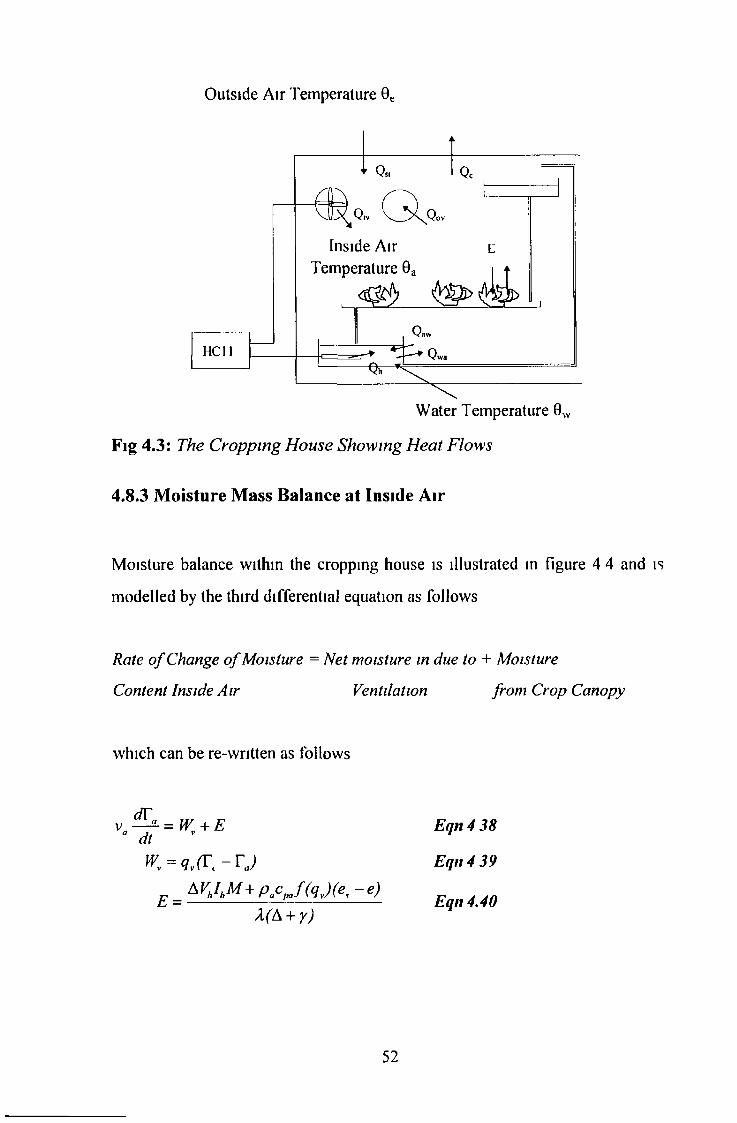
Outside Air Temperature 0e

Q,v Q . <Inside Air

Temperature 0;:rature ua i tc

HCll Q.

W ater Temperature 0W Fig 4.3 : The Cropping H ouse Show ing H eat Flows

4.8.3 M oisture M ass Balance at Inside Air

M oisture balance within the cropping house is illustrated in figure 4 4 and is modelled by the third differential equation as follows

Rate o f Change o f Moisture = Net moisture in due to + Moisture Content Inside Air Ventilation from Crop Canopy

which can be re-written as follows

rpvo — 2- = IV + E a dt E qn 4 38

E qn 4 39K = j

e A VhIhM + P ac J ( q v) ( e , - e ) A(A + y) Eqn 4.40

52

Outside Air Te

E

Inside Air f aHCll

Figure 4.4: 7% Cropping H ouse Show ing M oisture Flows

4.8.4 CO 2 M ass Balance in Inside Air

Finally, CO2 mass balance inside the cropping house is modelled by the fourth differential equation and supplementary equations as follows

Rate o f Change o fCO2 Cone = Net CO2 in due to Ventilation - CO2 lost to Crop due too f Inside A ir Photosynthesis

This leads to the following set of equations

V" ~dt = M ’~ M r K = 9,K-<P.)

E qn 4.41E qn 4 42

Eqn 4A 3

53

Outside Air Oe

Figure 4.5: The Cropping H ouse Show ing CO 2 F lows

4.9 Developm ent o f the M odel o f the Cropping House in the M atlab- Sim ulm k Sim ulation Environm ent.

The differential equations describing the model o f the cropping house were implemented as a script file in the M atlab/Simuhnk simulation environment ior windows Script files o f this type are called Matlab S-Functtom An S- function may be linked to a user-configured graphical interface using the Simuhnk simulation tool Figure 4 6 below, shows the Simuhnk block diagram used to process and display the input and output variables that affect and are affected by the model

54

0 00125

Flow Rate23

Fxt Air temp

40l td Hum

t a n M k Sp [

H eater M k Sp

100Incident light

Mux * f ( u )IMu\2 RII lo All

I 1 I --- Hf(») ,hPWM-Volts Tan C h a r

Mux ^ \p u 4Model

of VI» D

©-Clock

Dcrnux

Air Tem p

W a te r I emp

MuxI All to UN

+ 0(02timeI ime

Figure 4 6 Simulmk Block Diagram Showing the Cropping House with Changeable Inputs and Displaying Model Outputs

4.10 Steady State Characteristics o f the D eterm inistic M odel o f the C ropping H ouse

This section examines the steady state characteristics o f the model Using Matiab, a computer package for mathematical computation and simulation, the steady state form o f the model equations will be evaluated for a range o f input conditions A qualitative assessment o f the performance o f each element o f the model is given

The set o f graphs given in figure 4 7 are an indication o f how each variable in the model responds to external stimuli such as incident light intensity and external air temperature

4.10 1 Steady State Characteristic o f the Inside Air Tem perature

Figure 4 7 below shows the inside air temperature as a function o f ventilation rate and o f water temperature for the original model By setting the rate o f change o f Qa to zero, which is what happens under steady state conditions

55

5 9A lLa + U IKIIyAlimt + P a CpaA , L a,d.+ (5 9Ai+qiPacpa + VíAí)Oí

e.5 9A,L„ + UpnlyAumk + + 5 9 4 + 9i P(jC. j(i + {/ a

E qn 4 44which is a linear function of the nutrient solution temperature 6W and the external air temperature 6e if the ventilation rate qv is held constant This means that, the air temperature inside the cropping house 0a will increase if either nutrient temperature 0W, or external air temperature 0e, increase as in the real system The air temperature is a non-hnear function of ventilation rate as follows

A + B qv6 t6L = E qn 4 45C + B qvAs the ventilation rate q v becomes dominant, 0a asymptotically approaches 0e and this effect is independent of the value 0W, as shown below in figure 4 7

Figure 4 7 Steady State Inside Air Temperatili e Versus Ventilation Rate fo r Different Water Temperatures with Outside Air Temperature at (fC, and heater power at 400W

56

This is expected, since an increase in the ventilation rate in the real system will force more of the outside air into the cropping house, thus causing the internal air temperature to approach the outside air temperature

4 10.2 Steady State Nutrient Solution Temperature Characteristics

The steady state nutrient solution temperature is given by,

which means that 0W is a linear combination ol 0a, Qt, and 0e As belore, any increases in these quantities will result in an increase in the nutrient temperature

Any non-linearities in this equation come lrom the evaporation term XEt , which is a non-linear function of 0a as shown below

Consideration of equation 4 48 shows that XEC and thus 0W are linear functions of r a if the air temperature 0a and the ventilation rate q v are kept constant, since the equation is then of the form -

It is also apparent from equation 4 49 that as r a increases, the vapour deficit <v ea decreases, which decreases the evapo-transpiration rate XEt This agrees well with the real system

Q h + Q s , + 5 9 A t L a, + U poly A a n k +

/ p c. A I.

e,P a Cp „ A , L ,

E qna pa t at

r,4 .46

which is in the form,- Qh + A 0 a + B 6 l + C Eqn 4 47

AE =tAQ + 0 0 0 0 2 l ( l + q j [0a) F J 2 7 3 + 0 J )

217 J E qn 4 48

XEi =K, + K2{et - K3r a) E qn 4 49

57

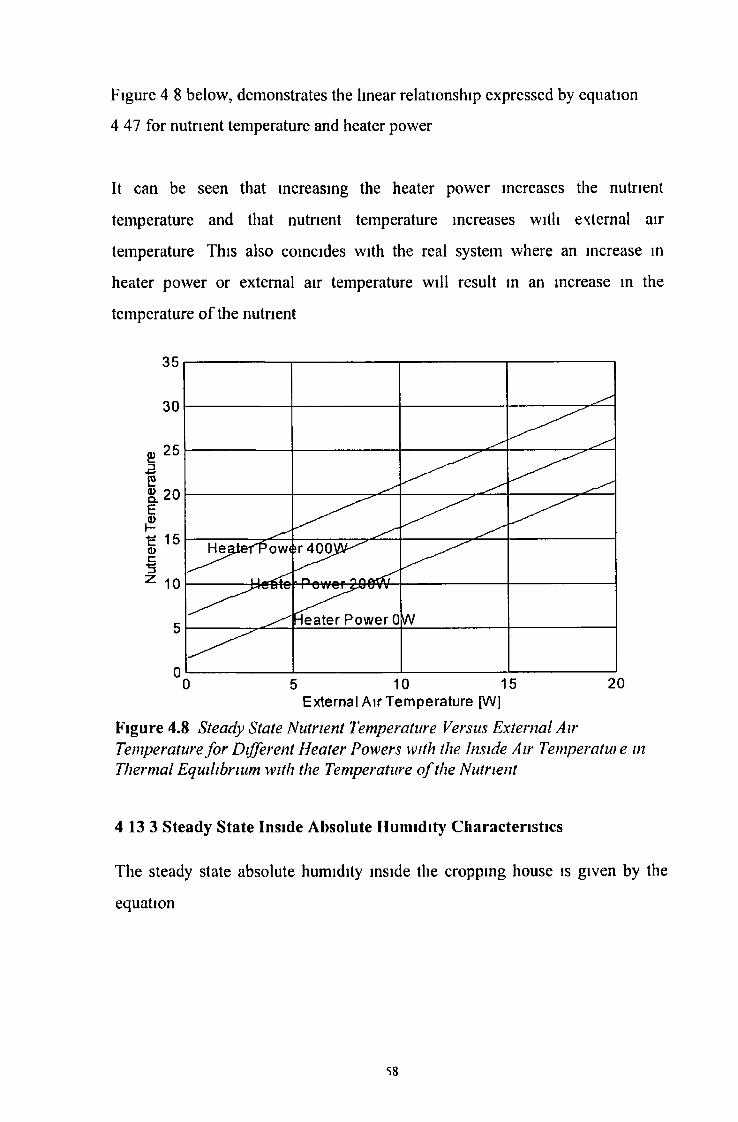
Figure 4 8 below, demonstrates the linear relationship expressed by equation 4 47 for nutrient temperature and heater power

It can be seen that increasing the heater power increases the nutrient temperature and that nutrient temperature increases with external air temperature This also coincides with the real system where an increase in heater power or external air temperature will result in an increase in the temperature o f the nutrient

External Air Temperature [W]

Figure 4.8 Steady State Nutrient Temperature Versus External Air Temperature fo r Different Heater Powers with the Inside Air Temper atui e in Thermal Equilibrium with the Temperature o f the Nutrient

4 13 3 Steady State Inside Absolute Humidity Characteristics

The steady state absolute humidity inside the cropping house is given by the equation

58

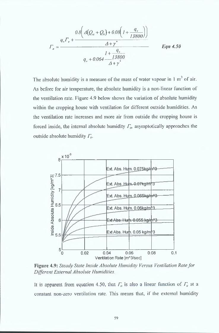
o l A(Qxi + Q ) + O m [ 1 + - ^ —1 V V h! V 13800)) q,re + -------------------------

r = -------------------------------------------------------------------------------------- Eqn 4.50a Qv

qv + 0.064-----A + y

The absolute humidity is a measure of the mass of water vapour in 1 m3 of air. As before for air temperature, the absolute humidity is a non-linear function of the ventilation rate. Figure 4.9 below shows the variation o f absolute humidity within the cropping house with ventilation for different outside humidities. As the ventilation rate increases and more air from outside the cropping house is forced inside, the internal absolute humidity r a, asymptotically approaches the outside absolute humidity r e.

8

FT 7.5 <E o>i *~q EI 6.5

1 oCO$ 6 0)£ 5.5

50 0.02 0.04 0.06 0.08 0.1

Ventilation Rate [mA3/sec]

Figure 4.9: Steady State Inside Absolute Humidity Versus Ventilation Rate fo r Different External Absolute Humidities.

It is apparent from equation 4.50, that r n is also a linear function of r c at a constant non-zero ventilation rate. This means that, if the external humidity

59

increases diffusion and ventilation ensure that the humidity inside the cropping house increases also

4,10.4 Steady State Inside C 0 2 Concentration Characteristic

The steady state C 02 concentration within the cropping house is given by,0qv0 ^ ^ L

0 a -------------— E qn 4 51<7v+-

r>

where the stomatal resistance rs is approximated by equation, 4 26-(?«

rv - 3000e 120which was introduced earlier in this chapter Consideration of equation 4 26 shows that 0 a is a linear function of 0 ei if q v and Q Si are kept constant, and a non-linear function of rs and q v Figure 4 10 below shows the effect of ventilation rate on the inside C 02 concentration for different incident light intensities using the above approximation for rs The inside C 02 concentration asymptotically approaches outside ambient concentration as the ventilation rate increases The higher the incident light intensity, the greater the photosynthetic uptake, which means that a greater ventilation rate is required to keep the C 02 concentration inside the cropping house near ambient levels This is also apparent from figure 4 10

Consideration of the set o f curves in figure 4 10 shows that the above approximation results in a C 02 concentration which is independent o f light intensity at a zero ventilation rate In the real unventilated system however, an increase in incident light, would result in a decrease in the C 0 2 concentration within the cropping house The solution to this problem is to assume 0 meso to be a linear function of the light intensity

60

A I W

SW Radiation Inside = 100W/mA2 SW Radiation Inside = 200W/mA2

SW Radiation Inside = 300W/mA2SW Radiation Inside = 400W/mA2

0 01 0 040 02 0 03Ventilation Rate [mA3/sec]Figure 4 10 Steady State Inside CO 2 C ontenu ation Veisus Ventilation Rate

fo r Different Levels o f Incident Solar Radiation

0 0 01 0 02 0 03 0 04Ventilation R ate [mA3 /se c ]

Figure 4 11 Steady State C 0 2 ConcenU ation versus Ventilation Rate fo r Different M esophyll CO 2 ConcenU ations

Figure 4 11 shows the result of taking &meso as a linear function of Qsl The coefficients for this approximations would need to be determined empirically and would result in secondary boundary conditions, which are beyond the scope

o f this work The original equation given by Rosenberg, Blad and Verma (1983), gives a good approximation o f the dynamic responses o f the real system as will be seen in the next section For the above reasons, the original approximation was selected to describe C 0 2 transfer

4.11 Sum m ary

This chapter has described a deterministic model o f a miniature cropping house, which was written in the M atlab/Simuhnk simulation environment It has also described and assessed the performance o f the model both qualitatively and quantitatively The next chapter will compare the behaviour o f the model o f the cropping house to the behaviour o f the real system with the same time-varying external climate It will point out weaknesses and suggest modifications which may be made to the model based on the results o f this set o f simulation experiments, and it will show the result o f other simpler modifications

62

C h a p t e r 5: M o d e l Validation b y C o m p a r i s o n with Real S y s t e m

5.1 Introduction

This chapter displays and assesses the dynamic responses o f the cropping house model This is achieved by applying historical input data measured at the real system to the deterministic model o f the cropping house and comparing the resulting modelled output data to the response data o f the real system

The first section describes the experimental set-up for the data acquisition, while the subsequent sections deal with the responses o f the differential equations o f the model to the quantities representing changing conditions outside the cropping house The last section shows an example o f how the model may be used to pinpoint improvements to the control system or the cropping house structure itself

5.2 Using Real H istorical Data to Assess the Perform ance o f the C ropping House M odel

A series o f three experiments was carried out on the miniature cropping house during the month o f September 1994 Quantities affecting the model o f the cropping house were measured over time on the real system These data were used to evaluate the performance o f the model by comparing the real measured data with the modelled output The comparison o f real and modelled data was accomplished by converting the raw data from the data­logger from M icrosoft Excel format to a series o f Matlab data files so that quantities corresponding to model input variables could be applied as inputs to the model It also allowed the quantities modelled by the simulation, such

63

as air temperature inside the unit, to be directly compared with the equivalent quantities measured in the real system

A description o f the data acquisition system is given in this section followed by an assessment o f the comparison between the real and the modelled data

I Data Logger | 1 leader TankFan Air Outlet

LightSensorHumiditySensor

RTD’s C02 SensorFig 5.1 : The Cropping H ouse with Controller and D ata-Logger

5.2.1 D ata -L o g ger and In stru m en tation

Figure 5 1 above shows the connections for the acquisition o f data using a data­logger The data logger used in this work was an RIL CL0008 programmable chart-logger Eight analogue input channels can be configured for connection to PtlOO R TD ’s, output voltages in the range 0-10V d c , or a selection o f output current ranges Data were stored temporarily in 256k o f battery-backed RAM during the trials and was later saved to a file on a computer via a serial link

64

The file format was compatible with Microsoft Excel which made it easy to transfer data to virtually any other package

5.2.1.1 Tem perature M easurem ent

Up to eight temperature measurements were taken simultaneously, although this depended on whether other parameters such as humidity, light level, and C 0 2 concentration were needed Due to the remote position of the Unit, it would have been impractical to log all these parameters using the 681IC11, since the micro-controller requires a computer to be positioned nearby to log data For this reason the data-logger was used, thus allowing the data to be stored temporarily in static RAM and saved to disk after the trials

Eight Pt-100’s were used to measure temperature They were hght-duty laboratory sensors with a stainless steel outer casing which is non-toxic

5 .2 .1.2 H um idity Sensors

The external humidity was measured using an RS humidity/temperature sensor with 0-1OV output (RS 256-253) This sensor accepted 0-12V d c supply voltage which made it suitable for measurements in the field as it could be connected to a 12V battery Humidities of up to 95% may be accurately measured using this sensor This was considered to be adequate lor external conditions The output voltage signal was sent via a twisted pair to the data­logger

Humidity inside the unit was measured using a form of psychrometer Two Pt 100 platinum resistance thermometers were laid in close proximity to each other One thermometer, called the dry-bulb thermometer, was positioned in

65

free air The second thermometer, called the wet-bulb thermometer was covered with damp gauze The wet-bulb thermometer reaches thermal equilibrium with the damp gauze surface which is cooler than the surrounding air because o f latent heat losses due to evaporation The difference in measured temperature between the two thermometers can be used to determine the humidity ol the air The advantage o f this measurement technique is that it cati measure humidities up to and including 100% relative humidity

5.2.1.3 CO 2 Sensor«

The CO 2 concentration was measured using the ADC W A-470B-E Carbon Dioxide Transducer, which also produces a 0-10V output In this case it was necessary to use a dc-dc converter to convert the d c output from the battery to the ±15V needed by the sensor The converter used for this purpose was a Computer Products NFC 10-12D 15

5 .2 .2 C on fig u ra tio n o f D ata L oggin g E q u ip m en t for the D a ta ­lo g g in g E xp erim en t and O ther B ou n d ary C on d ition s

The data-logging equipment as described above was used at the DIT college campus in Kevin Street Dublin on the 14lh o f September 1994, over the three day period including the 16th and 19th o f September 1994 and again on the 21st o f September 1994, to log data from the real system The parameters measured in the first one-day trial were as follows

• External air temperature• Inside air temperature,• Nutrient temperatures at the surface o f the weirs o f the top and bottom trays

on each side o f the cropping house

66

!

An average value for the nutrient temperature was calculated to match the uniform nutrient temperature o f the cropping house model

For the three day trial, the above quantities were measured in addition to humidity inside the cropping house

M easurements o f relative humidity and incident light intensity for the locality were obtained from the M eteorological Office in Glasnevin, Dublin Since these data were only available for hourly intervals, the information had to be modified to accommodate the faster sampling rate o f the data logging system which was 6 samples per hour

5.2.2.1 Experim ent to Investigate the Response o f System to a Step Change in H eater Power.

The first one day trial was used to obtain the response o f conditions inside the cropping house to a step change in heater temperature Before the trial started, conditions within the cropping house matched those outside Two 200 W heaters were turned on full as the trial commenced No ventilation was allowed as this would have dissipated much o f the heat generated by the heaters and reduced the air temperature lift (the difference between air temperatures inside and outside) o f the cropping house The accumulated data from this first trial are presented in figures 5 6 and 5 7

67

1

5.2.2.2 Investigation o f the Effect o f Changing Conditions over a Three Day Period

The three-day trial commenced with nutrient and air inside the unit in thermal equilibrium with temperature outside the cropping house At the start of the trial, the two 200 W heaters were once again turned on full and as before, the fan was kept off Thus the nutrient temperature and air temperature inside the cropping house were expected to rise at the start o f the trial and provide a temperature lift inside the cropping house

Figures 5 2 to 5 5 in the next section show historical temperature data from this first trial, along with the response to the model to the same input data Tigures5 8 and 5 9 show the variation of humidity over time for the same three day period

5.2.2.3 The Variation o f C 0 2 Levels over One Day

The final one-day trial was used to measure C 02 concentration in the cropping house The carbon dioxide sensor was calibrated using zero nitrogen and ambient C 02 levels in the air as zero and full-scale reference points respectively The C 02 sensor was connected to the data logger using an input configured for voltage signals between 0 V and 10 V Light intensity information for the one-day period was provided by the Meteorological Office, as in the first trial The sampling period for this experiment was set as before, at6 samples per hour

The fan was switched off for this experiment in order to observe and quantify changes in C 02 levels due to photosynthesis, in the absence of ventilation The

68

nutrient temperature in the tanks was thermostatically controlled by the water heaters within the temperature range 16°C to 20°C The data from this experiment are presented graphically in figure 5 10

5.3 Dynam ic Responses o f the Differential Equations Describing Conditions Inside the Cropping House

This section compares the performance o f the model with the performance o f the real system The following three sub-sections show the performance o f the original and altered elements o f the model in response to historical data from the real system In the following sub-section, the responses o f the nutrient and air heat balance equations in the cropping house are described The next sub­section deals with the moisture mass balance equation and the final sub-section describes the response o f the C 0 2 mass balance equation This section also describes the changes in the model which were required to improve its performance on the basis o f the comparison

5.3.1 D yn am ic R esp on ses o f the A ir and N u trien t S o lu tion H eat B a la n ce E q u ation s.

The nutrient heat balance equation has a larger time constant than the air temperature heat balance equation and it is this time constant which dominates the air temperature dynamics Figures 5 2 to 5 5 show the response o f the air temperature and water temperature to changes in the external environment It is apparent from the graphs that both the modelled and real data show a substantial reaction to the step change in heater power, which occurs at the start o f each plot

69

Consideration of equations 4 25 and 4 30 in the previous chapter shows that the water heater affects the nutrient temperature directly, whereas the air temperature is heated by sensible heat transfer Q wa from the plant and nutrient surface Any inaccuracies in the time constant therefore, may be attributed to problems with the dynamics of the nutrient surface temperature

The total volume of water nutrient mix used for the original model is 50 litres However, only a fraction of this solution comes into direct contact with the air inside the unit Consequently, the dynamics are much faster than those predicted by the model During normal operation it takes 10 litres of nutrient to fill the trays Setting the apparent volume of nutrient solution at 12 litres, makes the model respond well to changes in outside conditions such as air temperature However, as can be seen from figures 5 4 and 5 5, this value for water volume causes problems with the responses o f the model to the step change in heater power which occurs at the start o f the trial It appears that the water temperature is not uniform throughout the cropping house, as assumed for the original model

A solution to this problem is to introduce an additional first order differential equation in the model which will simulate a temperature lag between the nutrient temperature in the tank and the temperature at the nutrient and crop surface In this way the model can still be kept as a bulk parameter model which fits the original assumptions This alteration is left for future work

The second major difficulty with the model is also due to the temperature gradient between the header tank and the lower tray in the cropping house Tests show that in the real system, the surface temperature varies by about 3- 5°C under normal conditions The measured temperature shown in figures 5 3, 5 5 and 5 7 below are therefore calculated as the average o f four measurements of nutrient temperature taken at different points m the recirculation cycle

70

Figures 5 2 and 5 3 show the variation of the air and water temperature in the original model The effect of the heater on these variables in the original model is too great The heater efficiency in the original model is 95% However, to allow for the thermal gradients which exist within the cropping house, it is necessary to decrease this figure to an apparent efficiency o f 25%-27%

30

25

20

10

/Modelled

Air Temperature

Actual

151 Air Temperature

0 5 1 5Time [s X 10s]

2 5

Figure 5 2: M easu red R esponse o f A ir Temperature Inside the C ropping House to E xternal C onditions Between the 16th an d 19lh o f Septem ber 1994 an d the R esponse o f the O riginal M odel to Input D ata C ollected O ver the Sam e Time P eriod

71

TemPeratureDeg

2 5

Figure 5 3 Measured Response o f Nutrient Solution Temperature in the Cfopping House to External Conditions Between the 16th and 19th o f September 1994 and the Response o f the Original Model to Input Data Collected Over the Same Time Period

Reduction of the apparent volume of the nutrient in the recirculation system to 12 1 and the apparent heater efficiency to 25%, as recommended above dramatically improves the performance of the model as can be seen from figures 5 4 and 5 5 These changes result in what will be referred to as the m o d ified m odeI The modifications are a substitute for the inclusion of the additional differential equation

72

26

„ 24 /, \o ...< / VO)Q)QCD(0i_a>Q.E<Di - 2 0

14

j\%\ IActuaJ) /; 1

5 22 Air Temperature

18 Air Temperature

16

0 0 5 1 1 5 2 255Time [Secs]x 10

Figure 5 4* M easured Response o f A ir Temperature in the Cropping H ouse to E xternal Conditions Between the 16th and 19th o f Septem ber 1994 and the R esponse o f the M odified M odel to Input D ata C ollected O ver the Same Time P erio d

73

TemPeratureDeg

26

24

22

20

18

16

28

r V

Modelled

Nut Temperature

Actual

Nut Temperature

140 0 5 1 1 5

Time [sX105]2 5

Figure 5.5: M easured Response o f Nutrient Solution Tem perature in the R eal System to External Conditions Between the 1 6th and 19th o f Septem ber 1994 an d the R esponse o f the M odified M odel to Input D ata C ollected O ver the Same Time P eriod

Figures 5 6 and 5 7 show the response of the modified model and the real system to a step change in power applied to the heater of 0 W to 400 W on the 14th of September 1994 Air temperatures outside the cropping house at this time were at 14°C, and the fan was off It can be seen that the unventilated cropping house provides a lift in air temperature of approximately 6°C With full ventilation, the inside air temperature drops to the external air temperature

74

entTemPeratureDeg

Time [s X 10 ]

F igure 5 6* Measured Response o f Nutrient Solution Temperature In the Cropping House to a Step Change m Heater Power o f 0 to 400W on 14th September 1994 and the Modelled Response o f the Nutt lent Tempet ature in the Modified Model with Input Data Collected Over the Same Tune Period

75

T e mP e r a t u r eD egc Time [sX104]

Figure 5 7: Measured Response o f Inside Air Temperature in the Cropping House to a Step Change in Heater Power o f 0 to 400W on 14th September 1994 and the Modelled Response o f the Inside Air Temper atur e in the Modified Model with Input Data Collected Over the Same Tune Period

It is apparent from the above two graphs, that the time constant associated with the nutrient heat balance equation, which dominates the dynamics, is slightly larger than it should be This could be rectified by further decreasing the apparent volume o f the nutrient by roughly 20% It would be more correct however, to insert the additional differential equation mentioned earlier This is left for future work

76

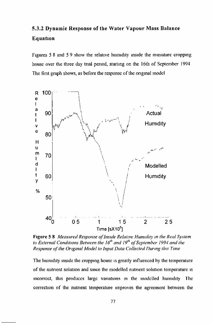
5 .3 .2 D yn am ic R esp on se o f the W ater V ap ou r M ass B a lan ce E q u ation

Figures 5 8 and 5 9 show the relative humidity inside the miniature cropping house over the three day trial period, starting on the 16th o f September 1994 The First graph shows, as before the response o f the original model

F igure 5 8 Measured Response o f Inside Relative Humidity in the Real System to External Conditions Between the 16th and 19th o f September Î994 and the Response o f the Original Model to Input Data Collected During this TimeThe humidity inside the cropping house is greatly influenced by the tem perature o f the nutrient solution and since the modelled nutrient solution temperature is incorrect, this produces large variations in the modelled humidity The correction o f the nutrient temperature improves the agreement between the

77

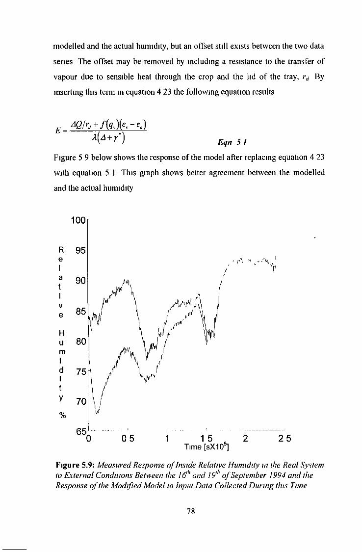
modelled and the actual humidity, but an offset still exists between the two data series The offset may be removed by including a resistance to the transfer of vapour due to sensible heat through the crop and the lid o f the tray, rd By inserting this term in equation 4 23 the following equation results

E AQIrd + f{q,){e<-ea)

*(à + r ') £ , » 5 1Figure 5 9 below shows the response of the model after replacing equation 4 23 with equation 5 1 This graph shows better agreement between the modelled and the actual humidity

Figure 5.9: M easured Response o f Inside Relative H um idity in the R eal System to External Conditions Between the 16th and 19th o f Septem ber Î994 an d the R esponse o f the M odified M odel to Input D ata C ollected D uring this Tune

78

The two plots stay within 5% of each other except where the modelled air temperature and nutrient solution temperature are inaccurate because of the problems with the dynamics of the nutrient heat balance equation which were discussed in the last section Even after this change however, it was found that the water vapour mass balance equation was sensitive to variations in temperature This element of the model requires more work to produce a robust and accurate humidity term It seems that the deterministic approach used in this thesis, is not suitable for describing humidity Deterministic equations describing humidity were found to be inaccurate or overly complex, often requiring information which is difficult to measure, such as resistances to vapour diffusion at the canopy An empirical approach, based on a simpler model structure is suggested as an alternative (Segincr and I evav 1971),(Young 1995) With accurate humidity sensors which measure high humidities, it should be possible to perform system identification to determine the coefficients o f simplified versions of equations 4 23 and 4 38 of the last chapter

5 .3 .3 D yn am ic R esp on se o f the C O 2 M ass B a lan ce E q u ation

A separate one-day trial was conducted to investigate the C 02 levels within the cropping house Figure 5 10 below shows the C 02 concentration within the cropping house on the 21st o f September 1994 and the response of the unmodified model There is an offset of 30 ppm between the real and modelled graphs This can be accounted for by the lack of a term describing respiration in the C 02 mass balance equation Monteith (1973) indicated that plants respire at a rate of 1 to 2 g CC^hr"1 independent of incident light levels

The main problem with any analysis of figure 5 10, is the fact that the C 02 sensor proved to be troublesome Since the accuracy of the sensor is not known

79

it is difficult to assess whether the model is perfonning well or the modelled CO 2 levels are coincidentally in the same range as those measured in the real system

The C 0 2 sensor was originally used on the three-day trial, but the data from the sensor had to be discarded after the sensor malfunctioned after a day o f operation It is assumed that the malfunction was due to the high humidities inside the cropping house The addition o f a dehumidifier on the input to the CO 2 sensor m ight solve this problem

CO2C0nc

nsIde

Cr0 P P1n9Hse

[ppm]Figure 510 The M easured CO 2 concent? at ion within the M iniature C ropping H ouse On the 21st Septem ber ¡9 9 4 and the Response o f the M odel with Input D ata C ollected O ver the Same Time Pet lod

80

The zero nitrogen required to calibrate the sensor was only occasionally available This is a practical problem which must be overcome before serious work on modelling C 0 2 fluxes is carried out It would also be beneficial if a more accurate measuring system could be arranged This would allow future researchers to perform more detailed analysis o f this part o f the model

5.4 U sing the M odel to Determ ine the Significance o f Heat Transfers within the C ropping House

This section is a demonstration o f a simple use o f the deterministic model o f the cropping house One o f the major concerns in any cropping house is where and how heat is being lost Using the modified model, the following information about heat transfers in the cropping house was obtained

With no solar radiation, zero ventilation, air temperature at 24°C, nutrient temperature 26°C, and external air temperature 16°C, the following modelled heat transfers were recorded

Qoc 41 5WQwc 1 1WQwca 0 2 WQwa 89 7 WQae 76 6 WQc 31 9 WQh 123 2 W

T able 5 1 Heat Flows in the Cropping House

The first observation about the above data is that the heat lost by conduction from the nutrient solution to the internal air Qnco and to the outside air Qwe, are significantly less than the other heat losses This is due to the thermal insulating polystyrene cladding around the nutrient reservoir tanks By comparison, the heat lost by conduction through the glazing Qoc is much greater

81

\ Though the heaters produce 400 W of heat, only 123 W arrive in the trays, 90 W are lost to the internal air due to convection from the heated nutrient surface Q wa This is desirable if the ventilation is kept low since the air is heated to a temperature above the external air temperature However if the fan were turned on high the resulting heat loss by ventilation would bring the air temperature and nutrient temperature to potentially unacceptable levels The majority of the rest o f the heat generated by the heater is dissipated by evapo-transpiration in the plant canopy E c

Quite a significant portion o f the heat inside the cropping house is lost by long wave radiation through the glazing This heat loss is difficult to reduce In general, the higher the optical transmission co-efficient the faster the plants grow However, high optical transmission coefficients usually mean comparatively large radiative heat losses also

Another interesting observation involves the existing fan in the cropping house Using equation 4 11, the equation which determines the heat lost through ventilation, for the same inside and outside temperatures and taking a maximum ventilation rate o f 73 Is-1, one obtains Qv = 0 0 7 3 (1 2 )(1 0 10 )(2 6 - 1 6 ) -884 WWhich means the original fan is capable of dissipating 884W of heat at full power This value is significantly larger the other heat losses outlined above, it appears that this fan is over-sized for the cropping house used in this work So based on the figures taken from the model, it is recommended that the present fan be replaced by a less one with a flow rate of 10 Is 1 as this would reduce the heat transfer due to ventilation Q v to around 100 W

82

This chapter has assessed the performance o f the model and its response to data from the real system Modifications based on the responses o f the original model and the behaviour o f the real system have improved its performance to an acceptable level The results from the modified model suggest that the inclusion o f an additional equation would improve the dynamic pcrlormancc ol the inside air and nutrient heat balance equations ih e moisture mass balance equation was found to be sensitive to the nutrient solution temperature and this equation requires further work The C 0 2 mass balance equation was the simplest o f the four and appeared to produce acceptable results The mam limitation with this final equation, involved the C 0 2 sensor which was difficult to calibrate and relatively unreliable

The next chapter will deal with the simulation o f the control system and the elements o f the real control system which was developed for the cropping house

5.6 Summary

83

\

Chapter 6: Control System for Vegetable Propagation Unit

6.1 In troduct ion

The overall purpose o f this project is to develop a digital control system for a miniature hydroponics plant growth unit The unit, which is called the vegetable propagation unit, is intended as an alternative to conventional vegetable growing techniques which will allow potential amateur growers with little growing space, to grow their own tomatoes, lettuce potatoes and other small-rooted plants It is envisaged that later versions o f the unit will be used as inexpensive tools for research into factors affecting crop production

The control system for the cropping house is similar to one produced by Claudia et al (1993), who developed a low cost Motorola 68000 microprocessor-based system for controlling the environment in a miniature glasshouse Claudia’s micro-controller monitored air temperatures at five different points in the greenhouse, humidity and C 0 2 concentration Air temperature was controlled using hot and cold water pumps whereas nutrient temperature in this work is controlled by a set o f electric water heaters In Claudia’s controller, fans were controlled in an on-off fashion rather than the variable speed control presented here Another feature which was similar to the controller in this work was a serial communication module which sent sampled data along a 100 m long serial link to a dedicated personal computer which logged the data Included in the monitor program on the personal computer was a feature which performed statistical analysis o f the data collected over one week

84

A block diagram o f the control system for the vegetable propagation unit is shown in figure 6 1 The control ler measures air temperature inside the unit, nutrient temperature and light intensity The first control led output is heater power which directly affects nu tnen t temperature and indirectly affects air temperature The second is fan power which affects the air temperature and the C 0 2 and moisture content o f the air

Figure 6 1 B lo ck D ia g ra m o f C o n tro l S ystem f o r the M in ia tu re C ro p p in g H ouse

This chapter will give a brief explanation o f heating and recirculation o f nutrient in the unit and will also discuss the ventilation system This will be followed by a description o f the controller hardware and development system and the data-logging system The controller software will be described under the headings oi luzzy logic expert control and PID control Finally, the response of the real system under control and the

85

response o f the simulated control system with the same boundary conditions, will be examined

6.2 T h e C onstruct ion and O peration o f the V egetab le&Prop agat ion Unit

This section will describe overall design and the explain the operation o f the miniature cropping house used for this study, which is called a vegetable propagation unit (VPU) The first sub-section will give an overview o f the VPU This will be followed by more detailed descriptions o f the ventilation in the unit and o f recirculation o f nutrient solution in the tanks and trays

6.2.1 D escr ip t ion o f the V egetable P ropagat ion Unit.

The vegetable propagation unit is a compact hydroponics-based vegetable cropping house The unit which is illustrated in figure 6 2, consists o f an A-frame structure on which six trays are suspended Three trays are positioned on each side o f the unit Two sump tanks at the base o f the unit and a single header tank at the apex fit into matching slots in the gable pieces The tanks are capable o f holding 56 litres o f nutrient but a typical value is around 36 litres

The gable ends are fixed to the tanks using a hand-tightened cross-wire which makes the unit rigid The ends are made from two layers o f fibre- glass which enclose 4 cm ot polystyrene foam to provide insulation The

86

slots for the tanks are constructed from welded strips o f Dexian During ventilation, a cavity in the centre o f the gable ends is filled with incoming air which passes through perforations in the inner layer o f fibreglass

The trays are positioned at an incline o f one in fifty A weir and reservoir at the top o f each tray provides a constant head of water which ensures that each tray receives a steady supply o f the water nutrient mix Excess water runs down the weir pipe in the centre o f each reservoir and into the next tray In this way, water cascades from the header tank at the apex o f the A-frame, through each set o f trays and into the two sump tanks in the base o f the unit A connecting pipe between the two sump tanks ensures that the water level in the base is kept balanced

Pumps located in each o f the sump tanks recirculate water returning from the trays The pumps are controlled by a float switch in the header tank which regulates the water level and ensures that water is evenly distributed between the sump tanks and the header tanks

Two 200 W aquarium heaters raise the water temperature in the header tank and are the only iorm of active heating in the unit A removable plastic cover on each tray minimises heat losses from the interior o f each tray and so protects the plant roots against low air temperatures

A small d c fan set in one gable end of the unit expels air from the interior thus drawing air from outside through a series o f perforations in the gables

87

6.2.2 Ventilation of the Vegetable Propagation Unit

The simplest form o f cropping house ventilation relies on natural ventilation from the outside air This may be achieved using a gauze cover through which ambient air is allowed to percolate freely Unfortunately, this means that spores and insects reach the loliagc ol the plants In addition, using this method, the incident light levels inside the unit are diminished and night temperatures are the same as external ambient temperatures

The introduction o f box section plastic glazing in place o f the gauze cover, and controlled ventilation in the form o f a small fan provides improved light levels while only allowing heat to escape the system when it is necessary to do so Control o f the fan speed facilitates control o f the air temperature as well as the C 0 2 and humidity levels within the unit A PAPST 12 W 12 V d c fan which could supply 100 litres per second was chosen for this purpose The speed control o f the fan will be addressed in the next section Air temperature is measured using a PtlOO RTD suspended inside the unit

6 .2 .3 N utr ient R ec ircu lat ion in the V egetab le Prop agat ion Unit

Tests conducted using a single pump to recirculate water from the sump tanks to the header tank at the top o f the A-frame resulted in the formation o f backwaters in the unit which meant under-utilisation o f

88

potential heat storage capacity A second pump was added to improve circulation and provide a fail-safe in the case o f pump failure

*

The full nutrient recirculation system is shown in figure 6 2 Nutrient is pumped to the header by the twin pumps mentioned above The incoming nutrient flows from the two sump tanks arc allowed to mix before directing them into the centre o f the header tank I his feature was added to minimise temperature gradients in the header tank

The pumps are switched by a float switch which is located in the header tank, and a mechanical relay This arrangement ensures that a constant head o f water is supplied to the trays below (Berry & Berigan 1993)

6,2 .4 N utr ien t F low within a Tray

Nutrient is allowed to propagate down through the trays from the header tank using a gravity feed system Figure 6 2 shows the nutrient How in a tray Nutrient enters the tray by a weir at the head o f the tray A small portion o f the nutrient flows through a small hand valve and down the length o f the tray Each tray is tilted to allow a gradient o f one in fifty, which is the preferred slope (Graves 1985) Excess nutrient flows over the weir where it is mixed with water returning from the end o f the tray before entering the reservoir o f the next tray

89

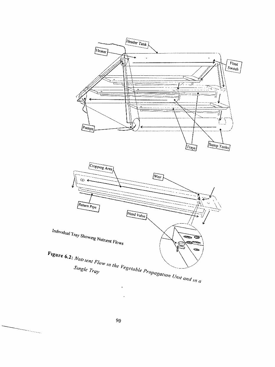
.-■gure 6.2: Nutrient Flow in the Vegetable Propagation Unit Single Traya n d i / i a

i

The simplest method for controlling nutrient temperature within the unit is to use two thermostatically controlled water heaters The problem with this scheme is that such healers icly on a thermostat within the heater casing itself to control the temperature Investigation o f a range o f 200 W commercial water heaters revealed that the thermostats typically controlled water temperature to within 1°C but not necessarily at the required temperature One water heater over-heated the water by up to 4°C

Initial data-logging o f the unit revealed that during normal operation o f the unit, there was typically a 5 to 10°C temperature drop between the nutrient immediately surrounding the heater and the nutrient in the bottom tray Furthermore, this temperature depends on outside air temperature and so is subject to disturbance changes Since the temperature in the trays is the controlled variable and not the temperature o f the water surrounding the heater, this method o f heating the nutrient is not suitable for this application

Using d ig i ta l c o n tr o l , and a temperature sensor located in the weir o f the bottom tray, it is possible to measure and control the water temperature in the trays directly Digital control also presents the additional advantage o f relating the nutrient temperature set-point to air temperature, time o f day, time o f year, phase o f cropping cycle and light levels With a correctly rated heater, it is also possible to keep temperature to within a fraction o f a degree o f the set-point temperature

6.2.5 Heating of Re-circulated Nutrient Solution

91

Accurate digital control for part o f the day, with a 5-10°C temperature lift at night can be accomplished using two o f the aforementioned heaters with their temperature settings on maximum Power to the heaters may be controlled using pulse width modulation The next section presents the Motorola MC68HC11 micro-controller integrated circuit, which is the device chosen to implement digital control for this work

5.3 M C 6 8 H C 1 1 M icro-con tro l ler Unit

This section summarises the main features o f the 68HC11 micro­controller unit (MCU) This is followed by a more detailed description o f the key elements o f the MCU, which are necessary for the operation o f a digital environmental controller

6.3.1 S u m m ary o f the E lem ents the 68 H C 1 1 -B a sed Digital C on tro l ler

Computerised systems are commonly used for climate control in modern greenhouses Udink Ten Cate (1983), identified northern European countries such as Ireland, Denmark and The Netherlands as places where the non-ideal external climatic conditions necessitated using a digital controller to regulate the environment within a greenhouse Digital controllers such as the one described here have found applications in many environmental control systems This controller is intended for a miniature cropping system and so must be relatively simple and inexpensive to produce

92

A simple schematic diagram of the controller hardware is shown in figure 6 3 Comparison with figure 6 1, shows how each output affccts the variables described in the mathematical model o f the last chapter

Air temperature and nutrient temperature are measured using two PtlOO RTD’s The resistance o f the R ID ’s varies linearly with temperature Two bridge circuits convert the resistances o f the R ID ’s to signals which are then amplified to voltages which are approximately proportional to temperature and are limited between 0 V and 5 V A light sensor measures the intensity o f solar radiation within the unit and supplies a third 0-5 V voltage signal The three analogue voltages are accepted by the micro-controller

Figure 6 3* S im p lif ie d re p re sen ta tio n o f D ig ita l C o n tro lle r H a rd w a re

A serial link to the P C allows data relating to the control performance o f the controller to be sent to the P C , where a program saves the data to '

93

disk Two PWM signals control the power to the water heater and fan by using an a c relay and an IGBT respectively to switch the currents to these controlled devices Four light emitting diodes are added for debugging purposes and for alarm indication

6.3.2 O v erv ie w o f the 68HC11 M icro -con tro l ler

The micro-controller used for this work is the Motorola MC68HC11E9, which is a member o f the 68HC11 family o f micro-controller integrated circuits The 68ITC11 is an 8-bit micro-controller with a nominal clock frequency o f 2MHz, which uses an extended version of the instruction set o f the 6800 family o f micro-processors The extended instruction set features instructions for multiplication and division o f integersAdditional on board facilities include -• 8 analogue inputs• 16-Bit timer-counter / time of day facility• Real time interrupt• Serial communication interface• Serial peripheral interface• Output compare to 16 bit free-running counter/timerFigure 6 4 shows the features available on the 68HC11 and which ports are influenced by each

The version o f the 68HC11 used in this work is called the 68H C11711E9CFS The E9CFS version o f the i c includes 12kB o f

94

EPROM, 512B o f RAM and 512B of EEPROM A more detailed(explanation o f this 1 c may be found in Motorola 1991a and 1991b

Fig 6.4 F ea tu res o f The 68H C 1 1E 9 M icro C o n tro lle r U nit

95

6.3.3 U sing the 68HC11 as a S tand-a lone M icro -con tro l ler

For this work, the 68HC11 micro-controller unit (MCU) was operated in single chip mode In this mode, the integrated circuit functions as a monolithic micro-controller without external address or data buses Port B, Port C, function as general purpose I/O, and Strobe A and Strobe B function as handshake lines This restricts total available memory to the capacity o f the MCU itself, which is 12288 Bytes o f ROM and 512 Bytes o f RAM Due to this memory restriction, the service routines have been implemented in 68HC11 assembly language to minimise stack usage and size o f controller code

The following sub-sections describe the main features o f the assembly level software» routines Flowcharts for these subroutines may be found in appendix B

6.3 .4 Sam p l in g o f T em p eratu re and Light Intensity

The 68HC11 includes an 8-channel multiplexed-input successive approximation analogue to digital converter (ADC), with a sample and hold circuit to minimise conversion errors caused by rapidly changing input signals Two dedicated lines (V RL and VRM) are provided as reference voltage inputs and these were connected to 0 V and 5 V respectively In the next section it will be seen that the control system was designed so that the analogue input voltage would not exceed these

96

voltage limits The ADC was configured to convert four o f the analogue input voltages in quick succession on receipt o f a CONVERT instruction The analogue to digital conversion was controlled by the assembly routine ADC

The sample time for the ADC was determined by the internal timer facility on the 68HC11 The timer has 16-bit free-running counter which is clocked by the output o f a programmable four stage prescaler which is in turn driven by the MCU E clock This counter is used by the micro­controller’s Real Time Interrupt (RTI) function to effect a periodic interrupt which can be used for sampling The slowest actual sampling rate permitted by the RTI function is 32 ms which is much too fast for monitoring or controlling relatively slow systems such as the miniature cropping house However, by only acknowledging every thousandth sample for instance, the effective sample time was lengthened The RTI- based sampling system was initialised by the subroutine RTIINI

6.3 .5 Serial C om m u n ica t ion s to the P.C.

The 68HC11 provides a full-duplex asynchronous Serial Communications Interface (SCI) with a standard NRZ format (one start bit, eight or nine data bits and one stop bit) and a variety o f baud rates The SCI facility was used to provide a data link to a personal computer if needed A low level routine called SCI transmitted blocks ol data from the controller to the Personal Computer at every sample instant

97

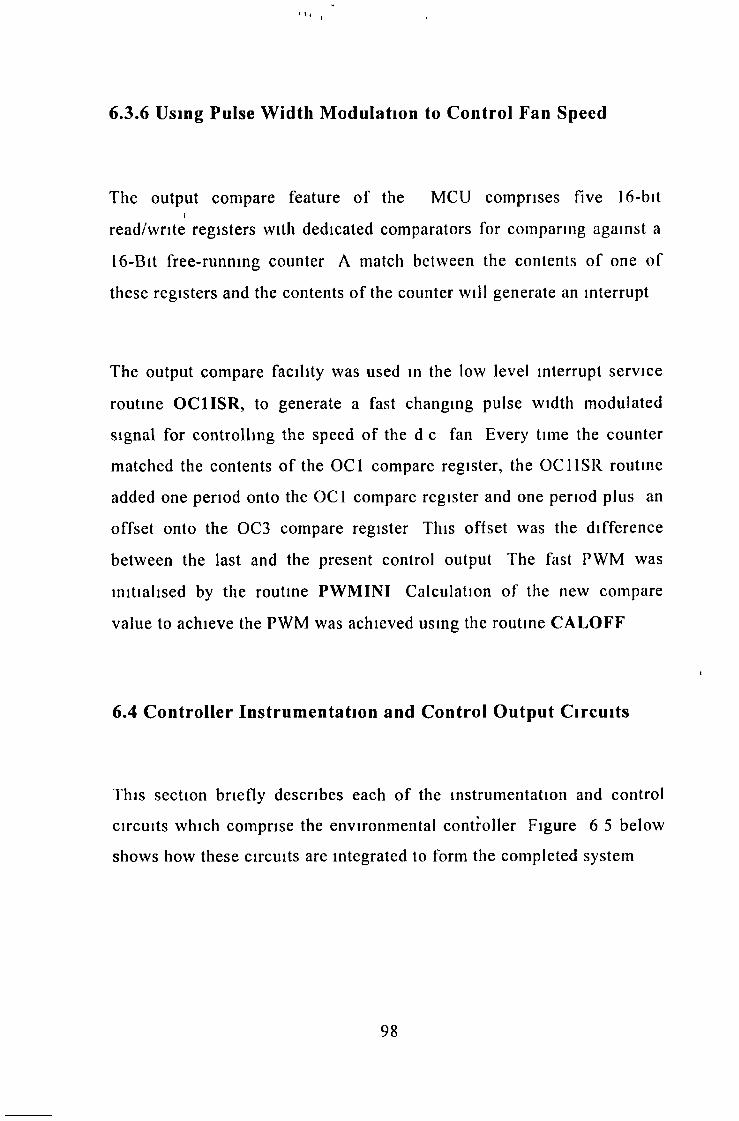
6.3.6 Using Pulse Width Modulation to Control Fan Speed

The output compare feature o f the MCU comprises five 16-bitIread/write registers with dedicated comparators for comparing against a

16-Bit free-running counter A match between the contents o f one o f these registers and the contents o f the counter will generate an interrupt

The output compare facility was used in the low level interrupt service routine OC1ISR, to generate a fast changing pulse width modulated signal for controlling the speed of the d c fan Every time the counter matched the contents o f the OC1 compare register, the OC1ISR routine added one period onto the OC1 compare register and one period plus an offset onto the OC3 compare register This offset was the difference between the last and the present control output The fast PWM was initialised by the routine PWMINI Calculation o f the new compare value to achieve the PWM was achieved using the routine CALOFF

6.4 C on tro l ler Instrum entat ion and Control O utput C ircuits

This section briefly describes each o f the instrumentation and control circuits which comprise the environmental controller Figure 6 5 below shows how these circuits are integrated to form the completed system

98

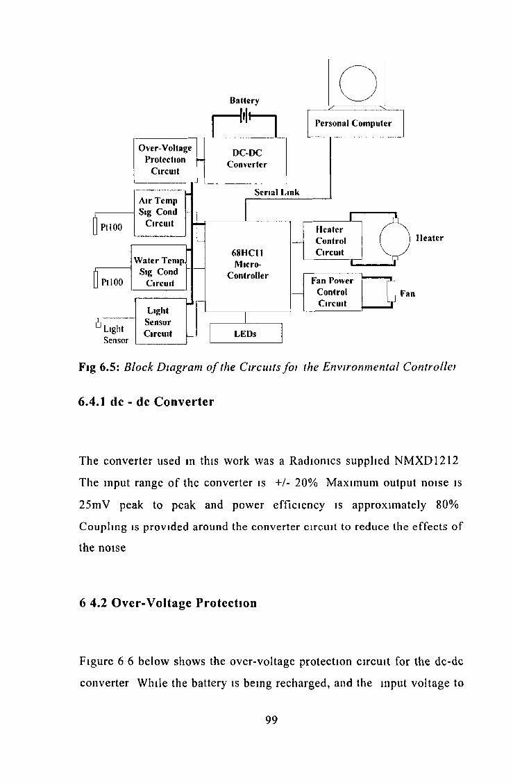
Fig 6.5 : B lock D ia g ra m o f the C ircu its fo r the E n v iro n m en ta l C on tro ller

6.4.1 dc - dc C on verter

The converter used in this work was a Radionics supplied NMXD1212 The input range o f the converter is +/- 20% Maximum output noise is 25mV peak to peak and power efficiency is approximately 80% Coupling is provided around the converter circuit to reduce the effects o f the noise

6 4 .2 O ver -V o ltage Protect ion

Figure 6 6 below shows the over-voltage protection circuit for the dc-dc converter While the battery is being recharged, and the input voltage to

99

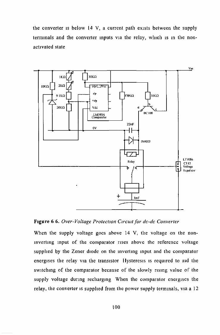
the converter is below 14 V, a current path exists between the supply terminals and the converter inputs via the relay, which is in the non- activated state

Figure 6 6. O ve r-V o lta g e P ro te c tio n C ircu it f o r d c -d c C o n v er te r

When the supply voltage goes above 14 V, the voltage on the non- mverting input o f the comparator rises above the reference voltage supplied by the Zener diode on the inverting input and the comparator energises the relay via the transistor Hysteresis is required to aid the switching o f the comparator because o f the slowly rising value o f the supply voltage during recharging When the comparator energises the relay, the converter is supplied from the power supply terminals, via a 12

1 0 0

V regulator and the relay The voltage at which the comparator switches can be altered by adjusting the potentiometer in the voltage divider

6.4 .3 M icro -con tro l ler O perat ing Frequency

An 8 MHz resonator was used to clock the processor This was considered to be preferable to using the internal clock for the following reasons• The resonator provides a much more stable oscillating frequency• It oscillates at 11 times the frequency o f the internal clock, thus

allowing the processor to carry out more operations per second

6.4 .4 T em p era tu r e Sensing Circuit

Two Platinum Resistance transducers were used in conjunction with Wheatstone bridges and instrumentation amplifiers to measure temperature The resistance o f these transducers varies directly withtemperature between 100Q at 0°C and 138 5fi at 100°C

The temperature monitoring was chosen to be within the range 0°C-40°C , which corresponds to a variation in resistance o f 15 54Q Resistor values in the bridge circuit were selected so that the maximum output voltage from the bridge was 0 1519V

101

This voltage, if inputted directly to the analogue to digital converter (ADC) circuit, would under-utilise the accuracy o f the ADC For this reason the signal was amplified, subject to the constraint that the maximum allowed voltage for the analogue input ports on the 68IIC11 is 5 V This requires an amplifier with a gain o f 33 Figure 6 7 below shows the resulting circuit

The two final stages in the temperature circuit arc to prevent the output voltage from the amplifier exceeding the 5 V limit and to filter any noise that may be transmitted to the 68HC11 The filter also serves to prevent any capacitive coupling between adjacent pins on the A/D The 5 V voltage limiter between the amplifier and the microprocessor consists o f a resistor and a Zener diode in series between common ground and the amplifier output which acts like a voltage divider but will actually limit the voltage into the processor to 5 V The Zener diode limits any over­voltages from the amplifier, (l e when the air temperature in the VPUgoes above 40°C), by drawing enough current to common ground, to keep the amplifier voltage output at 5 V

COMPONENTS A1 - ADJ625J Instrumentation Amplifier

Fig 6.7. T em p era tu re S en sin g C ircu it

102

6.4.5 Light Sensor

A Texas Instruments TSL250 Optical Sensor was used to measure light intensity This device produces an output voltage range o f 10 mV to 5 V with a supply voltage range o f 3 V to 9 V It is very sensitive to light with a responsivity o f typically 90 mV|.iW'1cm'2 The output o f this device was applied directly into an analogue input o f the MCU

6.4 .6 C ontro l O utput for H eater

The controller uses PWM to affect changes in the controlled variables A PWM signal with a period o f lm S is used to control the fan speed The signal controls an IGBT which sw itches the current to the fan A second PWM signal running at a frequency o f 0 5 Hz controls the heater current via a solid state relay

I2V

RELAY - MP240D4 (rarnell) Opto-Isolator - 4N25 Resistors 5% 25 watt

Fig. 6 8 : M CU Output Circuit fo r Controlling Heater Current

103

The controller output circuit for the heater which is shown above consists o f a comparator and opto-isolator which control an a c relay The heater used was a 200 W aquarium heater The relatively slow dynamics o f the heater enabled the use o f the slow PWM signal to control the water temperature

6.4 .7 C ontro l O utput for Fan C urrent

An insulated gate bipolar transistor (IGBT) was chosen to control the fan speed using the faster, output compare-based PWM signal This was for the following reasons

• The power requirements o f an IGBT are considerably lower than that o f a relay A typical mechanical relay draws 30 mA o f current when activated, this current is large when compared with the 1 mA drawn by an IGBT in the same circumstances

• IGBT’s are have a larger bandwidth and a longer mean time between failure than mechanical relays

• The cost o f using an IGBT is significantly lower than that o f a mechanical relay Snubber networks that are often used with IGBT's to limit di/dt and dv/dt are not needed in this case because o f the low voltages and currents, and the high ratings o f the IGBT's

Figure 6 9 below shows the fan speed control output circuit The fast output compare driven PWM signal is applied to the input o f the second comparator in the dual comparator integrated circuit The comparator output drives the opto-isolator which in turn switches the IGBT The IGBT controls d c current to the fan

104

12V (dc-dc Converter)

microprocessor

Components A1 2/4 LM 339 D1 IN5400 D2 RUR30I00 Resistors 5% 25 watt Opto-Isolator - 4N25 IGBT GT25J10I

-r- 0 47fjF

Fig 6 9 MCU Output Circuit fo r Controlling Fan Speed

6.4 .8 T h e C om p lete M icro-con tro l ler System

The connections between the MCU and the sensing and control circuits are shown in figure 6 10 The two light emitting diodes were included to supply “computer operating properly” signals and were initially used to test the PWM routines Pull-up resistors in the form o f 10 kQ resistor networks, were added to terminate unused MCU pins The Texas Instruments TL7705ACP i c was used to control reset o f the MCU

6.5 T h e Softw are D eve lop m en t System for the Digital E n viron m en ta l C ontro l ler

The software development system for the controller consisted o f eight basic elements

105

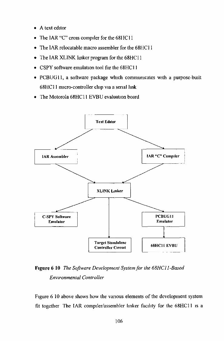
• A text editor• The IAR “C” cross compiler for the 6811C 11• The IAR relocatable macro assembler for the 68HC11• The IAR XLINK linker program for the 68HC11• CSPY software emulation tool for the 68HC11• PCBUG11, a software package which communicates with a purpose-built

68H C11 micro-controller chip via a serial link• The Motorola 68HC11 EVBU evaluation board

Figure 6 10 The Software Development System for the 68HCII-Based Environmental Controller

Figure 6 10 above shows how the various elements o f the development system fit together The IAR compiler/assembler linker facility for the 68HC11 is a

106

powerful tool which allows users to mix C source code for the 68HC11 with assembly level code IAR also supplies a compatible emulation tool for the 68H C11 called CSPY which was used for initial debugging o f the source code after link time

The 68I IC11 may be purchased as part o f an inexpensive development kit 1 his kit includes a 68I1C11 evaluation boaid tailed the 681IC11 EV13U, an assembler and an “Emulator” package for the P C , called PCBUG11, which communicates with the evaluation board via a serial link PCBUG11 does not provide all the services o f a full emulator, but docs allow some programs to be single stepped and can look at memory and at the contents o f registers Hus package was used for further debugging o f the C source and 68H C11 assembly code

6.6 C on tro l ler Softw are

6 .6.1 Introduct ion

The following sub-sections describe the software used in the controller to implement digital control oi the environment within the cropping house I he software may be divided into three main components which perform the following tasks -

• Assembly level service routines for serial communications, sampling o f data, and pulse width modulation

• Direct digital control o f nutrient solution temperature• Fuzzy expert control o f the environment in the cropping house Each sub-section below will deal with one o f these elements

107

The description o f the code in the last two sub-sections apply also to the simulated version o f the controller which is described in the next section

6.6.2 D irect Digita l Control o f N utr ient Solution T e m p era tu re

Control o f the temperature o f the recirculated nutrient solution was accomplished by using a digital PID controller which was written in “C” The control output value mn at each sampled instant can be calculated from the previous control output value mn and the last three control errors en, e„.| and en 2, using the following equation

tr if \ Ten Td(en ~ 2en-i + en-2)m n = m n -\ + K p \ { e n ~ e n- 1 ) + ~ J T + ----------------- ------------------- E qn 6.1

where Kp is the proportional gain, T is the sampling interval and T( and T(i are the integral and derivative action times respectively The advantage o f this form o f the digital PID algorithm is that the change m the controlled variable, mn-mn i can be applied directly as an input to a PWM waveform generator such as the one described in appendix B, thus reducing the amount o f computation required at run-time

In this work, the set-point for the digital PID controller was provided by the fuzzy controller A fuzzy controller is low pass in nature and the inputs to the fuzzy controller, which are light intensity and inside air temperature will not change suddenly The set-point for the digital PID controller will therefore change slowly and so derivative kick is reduced

The control system may be considered to be a form o f cascade control, with the higher level fuzzy controller providing the set-point for the PID controller, as may be seen from consideration o f figure 6 1 at the start o f this chapter The structure o f the controller represented by equation 6 1 is similar to ones

108

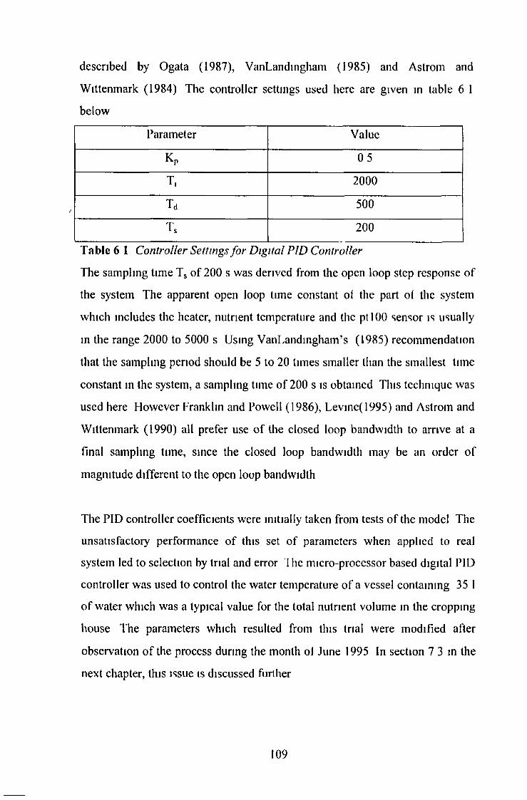
described by Ogata (1987), VanLandingham (1985) and Astrom and Wittenmark (1984) The controller settings used here are given in table 6 1 below

Parameter ValueKP 0 5T, 2000Td 500Ts 200

Table 6 1 Controller Settings fo r Digital PID ControllerThe sampling time Ts o f 200 s was derived from the open loop step response o f the system The apparent open loop time constant ot the part oi the system which includes the heater, nutrient temperature and the ptlOO sensor is usually in the range 2000 to 5000 s Using VanLandingham’s (1985) recommendation that the sampling period should be 5 to 20 times smaller than the smallest time constant in the system, a sampling time o f 200 s is obtained This technique was used here However Franklin and Powell (1986), Levine(1995) and Astrom and Wittenmark (1990) all prefer use o f the closed loop bandwidth to arrive at a final sampling time, since the closed loop bandwidth may be an order o f magnitude different to the open loop bandwidth

The PID controller coefficients were initially taken from tests o f the model The unsatisfactory performance o f this set o f parameters when applied to real system led to selection by trial and error The micro-processor based digital PID controller was used to control the water temperature o f a vessel containing 35 I o f water which was a typical value for the total nutrient volume in the cropping house The parameters which resulted from this trial were modified after observation o f the process during the month ot June 1995 In section 7 3 in the next chapter, this issue is discussed further

109

6.6.3 C ontro l o f Aerial E n vironm en t Using Fuzzy Logic .

Control o f the climate within the cropping house was accomplished with the help o f a fuzzy logic-based expert controller Traditionally, commercial growers have controlled the environment inside greenhouses by opening vents and switching boilers using rules based on the external climatic conditions In general for instance, the higher the incident light intensity at the plant canopy, the higher the desired air temperature, since a plant photosynthesises more efficiently at higher ambient air temperatures, below a threshold o f approximately 26°C

This example can be converted to the following fuzzy rule

IF LIGHT INTENSITY IS HIGH, THEN MAKE WATER TEMPERATURE SET-POINT HIGH

In this way, the degree to which the light intensity is HIGH, determines the degree to which the water temperature set-point should be made HIGH also

Probably the most crucial stage in designing a fuzzy controller is the acquisition o f the expert knowledge o f the system required for the creation o f the rule-base and sets o f the fuzzy controller The knowledge required for creation o f the rule-base and sets was acquired in the following way

• A set o f rules similar to the one shown above were first compiled after an informal discussion with a plant physiologist and an experienced grower

• The information was supported by reference to texts on plant physiology Table 2 1 in chapter 2 shows a summary o f the results o f this search

110

• The rule-base was then tested on the deterministic model o f the system to see how it would perform

• Finally, the sets and rules were tested on the real system by running the controller continuously for four days and monitoring its performance

1 he lollowing three main control rules were lormulatcd lor the luzzy controller

Control Rule #1

If air temperature is very high then turn fan on high and nutrient temperature lowJustification Plants die after prolonged periods o f temperatures which exceed 26°C

Control Rule #2

If the air temperature is very low, then make nutrient temperature high and turn fan o ffJustification Plants die if temperatures drop near to freezing Heaters can only provide an appreciable temperature lift if the fan is o ff

Control Rule #3If the above two conditions are not met then keep nutrient solution temperature at approximately 24°C and keep the unit well ventilated Higher light levels will need higher ventilation ratesJustification The mam considerations during the day are cooling the cropping house and keeping the C 0 2 levels high and humidity low At night howeverrespiration involves a much lower mass transfer rate than photosynthesis and

/the main concern is to keep the cropping house heated so the ventilation should be kept low

111

Using the above control rules, the fuzzy sets and fuzzy rule-base shown below were created to effect control of the model and of the environment in the cropping house The selection of ranges for the controller inputs and outputs is derived from experience gamed in initial trials with various prototypes o f the cropping house between May 1993 and August 1994 The temperature range selected for the two pt-100 RTDs was 0°C to 40°C as the temperatures in the cropping house only transcends these limits in the most extreme conditions

Light sensors for horticulture usually associate a spectral band with light intensity figures A range of 0-250 W m2 was found to be applicable to the bandwidth of the ORP 12 when used with lettuce plants

In appendix A, the voltage-speed characteristic o f the fan is derived The data sheet for the fan states that the fan will not operate for applied voltages which are lower than 5 V In fact, the fan operates when the applied voltage is kept between 3 5V and 12 V which corresponds to 30% to 100% of full fan power However since the fan was overrated, it was required to operate at no higher than 50% of full power as seen below If required fan power dropped below 30%, the fan stopped The nutrient temperature set-point for the PID controller was allowed to vary between 19°C and 27°C

Note that the outermost sets of the output universes appear to exceed their boundaries This is because control action resulting from each of these outermost output sets never exceeds the centre of gravity of those sets Lyons (1993)

112

0 5 15 25

Inside A ir Temperatiti e ¡°C ]4 0

Incident Light Intensity [W m 2]

Fan Power [% ]

N utrient Solution Temperature Set-point ¡°C ]

Figure 6 11. Input and Output Universes o fD isco u t se fo r Fuzzy Conti allei The rule-base for the fuzzy controller is shown below

113

If Inside Air Temperature is low and Incident Light Intensity is low then set Nutrient Temperature Set-pomt high and Fan Power low

If Inside Air Temperature is low and Incident Light Intensity is m oderate then set Nutrient Temperature Set-pomt m oderate and Fan Power m oderate

If Inside Air Temperature is low and Incident Light Intensity is high then set Nutrient Temperature Set-pomt m oderate and Fan Power m oderate

If Inside Air Tem perature is m oderate and Incident Light Intensity is low then set Nutrient Temperature Set-point m oderate and Fan Power m oderate

If Inside Air Temperature is m oderate and Incident Light Intensity ism oderate then set Nutrient Temperature Set-pomt m oderate and Fan Powerm oderate

If Inside Air Temperature is m oderate and Incident Light Intensity is high then set Nutrient Temperature Set-point m oderate and Fan Power m oderate

If Inside Air Temperature is high and Incident Light Intensity is lowthen set Nutrient Temperature Set-point m oderate and Fan Power m oderate

If Inside Air Temperature is high and Incident Light Intensity is m oderate then set Nutrient Temperature Set-pomt m oderate and Fan Power m oderate

If Inside Air Temperature is high and Incident Light Intensity is high then set Nutrient Temperature Set-point low and Fan Power high

The above set of fuzzy rules are presented in tabular iorm in table 6 2 below

114

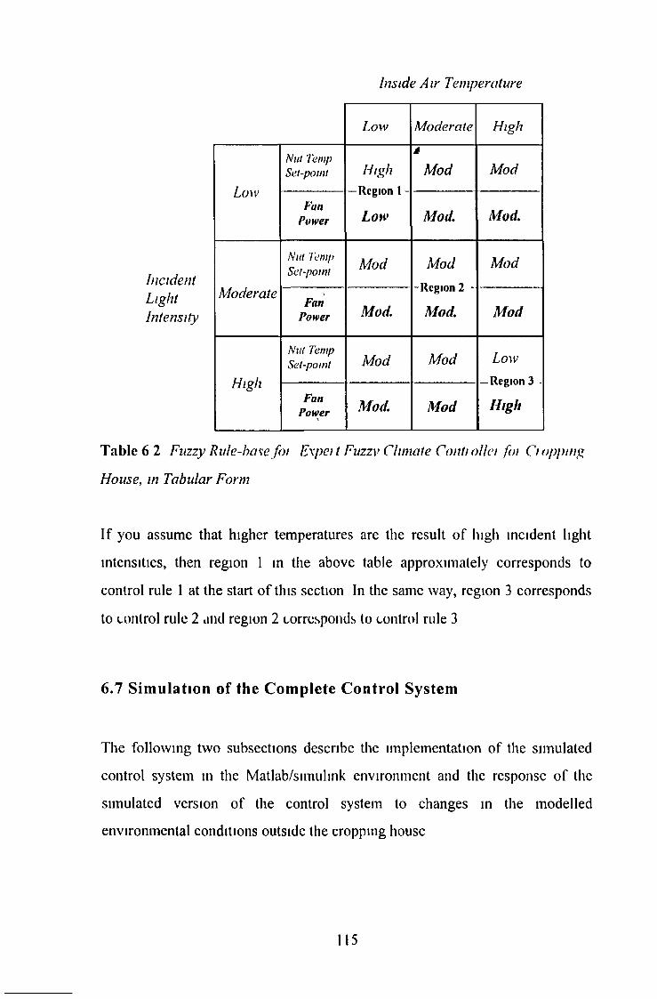
Inside A ir Temperature

IncidentLightIntensity

Low M oderate High

Low

Nut Temp Set-point High

—Region 1 -L o w

*M od M od

FanPower M o d . M o d .

M oderate

Nut Temp Set-point M od M od

-Region 2 -M o d .

M od

FanPower M o d . M o d

High

Nut Temp Set-pomt M od M od Low

—Region 3 -H ig h

FanPower%

M o d . M o d

Table 6 2 Fuzzy Rule-base fo i Expei t Fuzzy Climate Conti olici fot O oppmg House, in Tabular Form

If you assume that higher temperatures are the result o f high incident light intensities, then region 1 in the above table approximately corresponds to control rule 1 at the start of this section In the same way, region 3 corresponds to control rule 2 and region 2 corresponds to control rule 3

6 .7 S im u la tio n o f th e C o m p le te C o n tr o l S y ste m

The following two subsections describe the implementation of the simulated control system in the Matlab/simuhnk environment and the response o f the simulated version of the control system to changes in the modelled environmental conditions outside the cropping house

115

6.7,1 Description of the Simulated Control System as

Implemented in Matlab/Simulink

The fuzzy controller was tested in simulation by implementing it as a simulation in the MATLAB Simuhnk environment The following Simuhnk block diagram shows the simulation layout The three main elements in the simulation are three Simuhnk S-functions as listed below

• Mathematical Model describing the climate inside the cropping house written as an S-function

• S-function implementation of the digital PID controller• S-function implementation of the expert fuzzy controller

One of the reasons for developing the model was to test the performance of the control system without having to perform tests on the real plant

Figure 6.12 Simuhnk Block D iagt am Showing the C om plete C ontrol system fo r the C ropping H ouse and D isplaying M odel Outputs

116

The remote location of cropping houses makes them ill-suited to intensive experimental work such as system identification For this reason a model was developed to support any physical experiments and to permit efficient optimisation of any new control strategy A simulink block diagram ol the controller is shown in figure 6 12 Consideration of the block diagram shows how the fuzzy controller forms an outer loop with the PID nutrient temperature controller forming the inner loop

In order to carry out tests on new control strategies or re-designs of the cropping house, the controller was implemented as MArLAB-Simulink S- F un cttons For this work, two S-functions were created to model the controller The first was a simulated version of the open loop fuzzy logic expert controller discussed earlier, which performs some of the tasks carried out by a grower in a conventional growing house This controller measures light intensity and air temperature and makes decisions about the heating and ventilation requirements of the house The decisions influence the two outputs of this simulated controller which are nutrient temperature set-point and fan power

The nutrient solution temperature set-point was taken as an input for the second S-function which simulated the digital PID controller introduced in the last section This controller measured the nutrient solution temperature and attempted to keep it at the desired set-point value which had been provided by the fuzzy logic expert controller block

The S-function implementation of the model of the system was incorporated into the simulation as the “F uzzy C on tro l” and “D ig P ID ” s-function blocks of figure 6 12 so that the two controllers controlled the model in simulation

Three “A D C ” blocks simulated the eight bit analogue to digital converter feature of the Motorola 68HC11 micro-controller This was accomplished by

117

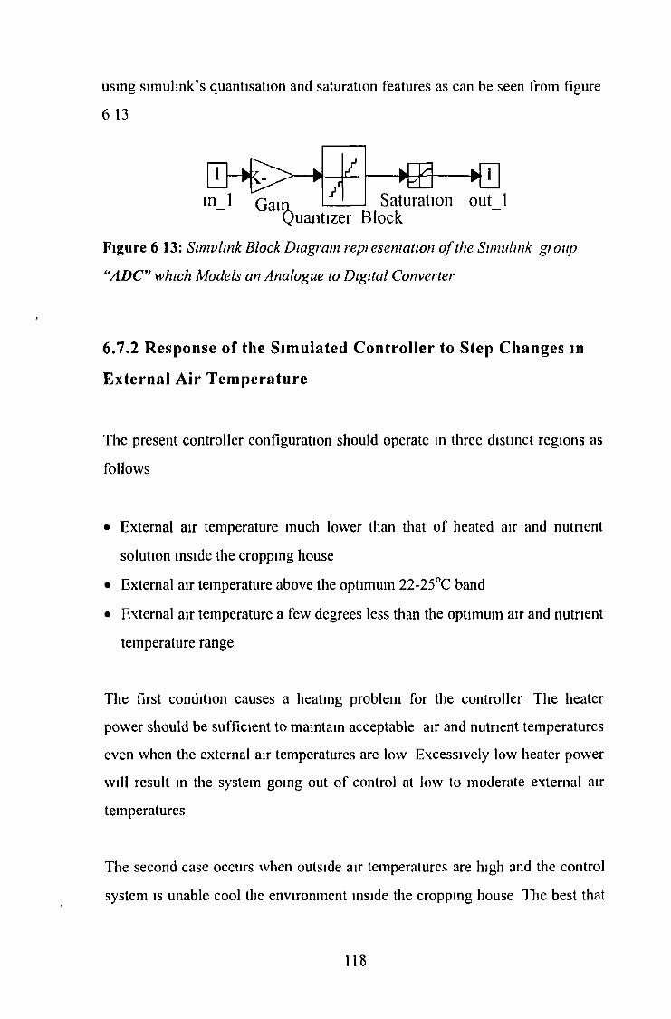
using simuhnk’s quantisation and saturation features as can be seen from figure 6 13

Figure 6 13: Simulmk Block D iagram representation o f the Simuhnk g fou p “A D C ” which M odels an Analogue to D ig ita l Converter

6.1JI Response of the Simulated Controller to Step Changes in External Air Temperature

The present controller configuration should operate in three distinct regions as follows

• External air temperature much lower than that of heated air and nutrient solution inside the cropping house

• External air temperature above the optimum 22-25°C band• External air temperature a few degrees less than the optimum air and nutrient

temperature range

The first condition causes a heating problem for the controller The heater power should be sufficient to maintain acceptable air and nutrient temperatures even when the external air temperatures are low Excessively low heater power will result in the system going out of control at low to moderate external air temperatures

The second case occurs when outside air temperatures are high and the control system is unable cool the environment inside the cropping house The best that

118

can be achieved by the controller with the existing controller outputs is to switch off the heating system

Finally, the last case corresponds to the system being in control when the air temperature and nutrient temperature inside the cropping house should be slightly less than optimum This means that only a slight temperature lilt is required to bring the temperatures within the optimum range

Figure 6 14 below shows the simulated controller responses to step changes in external air temperature

32

30

oo>q 28<DL a3

• MCD

&. 26E<Dt-

24

22

20

180

Ext Air Temp =30 Deg C

Ext Air Temp =25 Deg C

Ext Air Temp =20 Deg C

Ext Air Temp = 15 Deg C\ \ \ \

Ext Air Temp =10 Deg C

2 3Time [Secs]

4 5x 10

Fig 6 14 Sim ulated Responses o f Conti o iled Nutrient Tem perature to S tep Changes in External An Temperatui e

119

The water heater cannot provide enough power to heat the nutrient to the required temperature of 24°C when the external air temperature is below 15°C The curve showing the response to an external air temperature oi 10°C is a typical example The heater can only provide a temperature lift of 9°C, which means that the water temperature cannot exceed 19°C and thus never reaches the set-point temperature This corresponds to case one above

The second case is represented by the curve where external air temperature is at 30°C This means that the air temperature outside the cropping house exceeds the optimum temperature range inside the cropping house Since there is no active cooling device such as a heat exchanger available to cool the incoming air, the nutrient temperature tends to rise towards the external air temperature of 30°C

The final class of curve represents external air temperatures in a range which allows the nutrient temperature to be controlled For a nutrient temperature set- pomt of 24°C, this occurs when the external air temperature is within the range 15°C- 24°C The curves representing external air temperatures of 15°C and 20°C are in this category It can be seen from these response curves that they are within 1°C of 24°C which is the set-point temperature

Since the present control configuration only operates correctly for external air temperatures above 15°C, it can be concluded that higher power heaters are required to ensure that the temperatures inside the cropping house are adequate Based on the fact that the present total heater power is 400 W, an additional 600-800 W of power would be needed However this amount of power is expensive to provide with electric heaters So based on recommendations resulting from this study, and for reasons of safety the electric heater system is to be replaced with a more powerful gas/oil burner-based water heating system

120

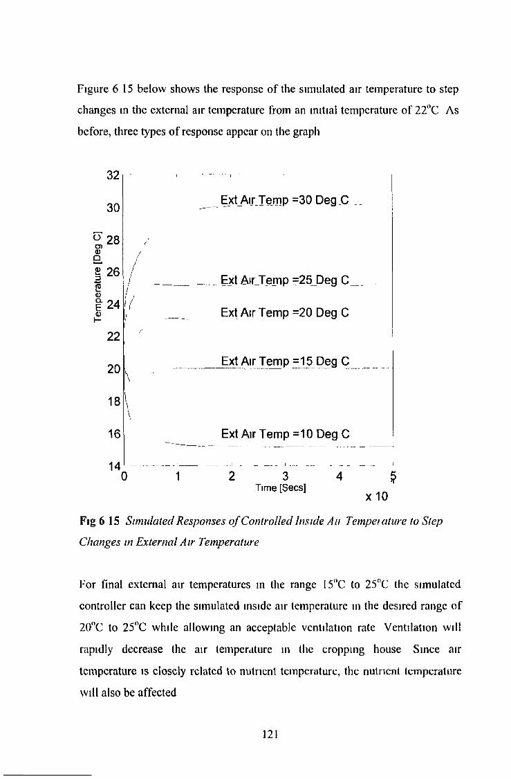
Figure 6 15 below shows the response of the simulated air temperature to step changes in the external air temperature from an initial temperature of 22°C As before, three types o f response appear on the graph

32

30

^ 28 O)<DQ§ 262<DI 24a)

222018

16

140

Ext_Air.Je.mp =30 Deg C

Ext AirTemp =25 Deg C

Ext Air Temp =20 Deg C

Ext Air Temp =15 Deg C

Ext AirTemp =10 Deg C

2 3Time [Secs]

4 §x 10

Fig 6 15 Sim ulated Responses o f C ontrolled Inside An Temperature to Step Changes in E xternal A ir Temperature

For final external air temperatures in the range 15°C to 25°C the simulated controller can keep the simulated inside air temperature in the desired range of 20°C to 25°C while allowing an acceptable ventilation rate Ventilation will rapidly decrease the air temperature in the cropping house Since air temperature is closely related to nutrient temperature, the nutrient temperature will also be affected

121

For satisfactory internal air temperatures when air temperatures outside the cropping house are low, it would be necessary to introduce some form of air heating device in addition to the proposed water heater Some possible air heating devices are described in the next chapter Using the existing control configuration, the air temperature must be above a threshold temperature bclore the air temperature stays within the desired range

For external air temperatures above 25°C, region 1 of the fuzzy controller rule- base ensures that the electric water heaters are switched off and the fan ventilation rate is set high This ensures that there is no temperature lift inside the cropping house as can be seen from the curve representing conditions when external air temperatures are at 30°C

6 .8: Im p lem en tat ion o f the Contro l ler for the 68HC11 M ic r o ­contro l ler

To allow the controller code to be used on the real plant, the fuzzy controller and digital PID controller were implemented in the “C” programming language for the 68HC11 The controller code was written so that the PID controller settings and the control rules and fuzzy sets for the fuzzy controller would be identical to those used in the simulated controller written for Matlab The code was compiled, assembled and linked using the software development system described earlier in this chapter The first of the following three subsections describes the sequence of operation of the code The second subsection deals with execution time and memory requirements The final subsection briefly discusses how the code was tested in the development stage

122

6.8,1 Sequence o f Operat ion o f C on tro l ler Code?

The sequence of operation of the code on the micro-controller is as follows Voltages corresponding to temperatures and light intensities are first sampled by the sampling service routines Sampled values from the A D C ’s are converted into floating point format after each sample instant All the internal calculations for the two controllers are performed by using floating point arithmetic Calculated control output values corresponding to P W M mark-space ratios, are converted back to integer format The P W M service routines then convert the integer to P W M signals for the fan and heater The sequence of execution of the various elements of the controller code is shown in figure 6 16 below

Figure 6.16 Sequence o f Execution o f Conti oiler code

6.8.2 Execut ion time and M em o ry R eq u irem en ts for the C on tro l ler

The software for the controller when actually resident on the micro-controller integrated circuit, occupies approximately 8 5 kBytes ol EPROM I his leaves 3 5 kBytes of EPROM for further development In addition, by using integer arithmetic in place of floating point arithmetic, the amount of memory required could be much reduced Extra inputs could easily be added to the fuzzy controller since the controller may need as little as four Bytes to store one fuzzy set and for n inputs and m outputs, needs only 2 +2(n+m) Bytes per rule The

123

512 Bytes of RAM available on the 681IC11E9 are used for the stack and for storing variables This leaves the 512 Bytes of EEPROM free for other uses Typical examples would be as a data storage space in case of emergency shutdown or for data-logging In a later version of the controller it could be used to store modifications to the original rule-base This would allow the rule- base to be reprogrammed on-site via the serial link to a laptop computer for instance

The code takes milliseconds to go through one complete cycle This execution time is orders o f magnitude less than the sample time of 200 s, so it is possible to add extra code for intelligent data-logging or more complex fuzzy control for instance, without timing constraints

6.8.3 O ther C om m en ts on the Im plem entat ion and T est ing o f the C on tro l ler

In the development stage of the project, low-level routines were tested by moving them to RAM where they could be single-stepped for debugging purposes Interrupt vectors were located as pseudo-vectors in RAM during the design stage and were finally moved to the last few Bytes of EPROM High level routines such as the PID controller and the fuzzy controller were tested by first compiling and run-time testing using Borland Turbo-C They were then re­compiled for the 68HC11 and tested with the assembly routines The full controller was then further tested by attempting to control the temperature in a tank of water, before being transferred to the real system This control was successful (Berry and Berrigan 1994)

Prior to testing the expert controller on the real system, the expert fuzzy controller was tested statically by changing the temperature measured by the

124

two Pt 100’s and the light incident on the light sensor and observing the change in fan speed and the temperature of a water container in which the heaters were immersed (Berry and Berngan 1994)

6.9 Perform ance Trials o f the Expert Fuzzy Contro l ler on the Real System and on the S imulated System

This section gives an assessment of the performance of the controller based on the results o f a four day trial on the real system The first sub-section presents the result o f the trial on the real system The second sub-section shows the output o f the model which results from temperature data from the above trial being applied to the cropping house model

6.9.1 C on tro l ler Perform ance Trial on the Real System

In June 1995, the controller was set up to control the environment in the cropping house The remote location of the cropping house during the course of the trial meant that a personal computer could not be located sufficiently close to use the serial link capability For this reason, the data logger set-up identical to that described for the three day trial at the beginning of the previous chapter was used to monitor the performance of the controller Temperatures at four points in the nutrient circuit were monitored, as were external air temperature and air temperature inside the cropping house

Problems with humidity sensors and the CO2 sensor meant that the humidity and C 02 levels could not be measured reliably either inside or outside o f the cropping house, These aspects of the control system model have therefore been ignored

125

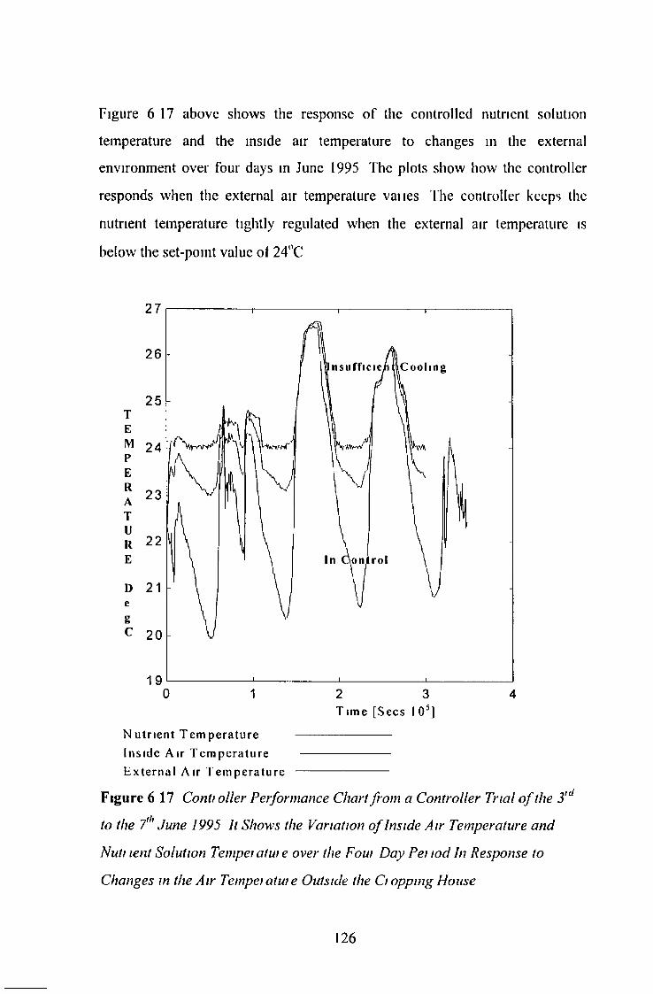
Figure 6 17 above shows the response of the controlled nutrient solution temperature and the inside air temperature to changes in the external environment over four days in June 1995 The plots show how the controller responds when the external air temperature vanes The controller keeps the nutrient temperature tightly regulated when the external air temperature is below the set-point value of 24°C

Tim e [Secs 1 0 5]Nutrient Temperature -------------------------Inside Air Tem perature ------------------------External Air Temperature ------------------------

Figure 6 17 Controller Performance Chart from a Controller Trial o f the 3,dto the 7th June 1995 It Shows the Variation o f Inside Air Temperature andNutt tent Solution Temper atur e over the Four Day Per tod In Response toChanges in the Air Temper atur e Outside the Cr opping House

126

If the external air temperature and hence the inside air temperature exceed this value, which happens when the fuzzy controller is operating in region 1, the controller cannot cool the air and this in turn heats the nutrient solution Tor external air temperatures below 24°C and above 15°C , the heater can provide enough temperature lift to heat the water This represents operating region 2 for the fuzzy controller As can be seen from the graph, external air temperaturedoes not drop below 15°C at any point

The inside air temperature stays close to the optimum value of 24°C when theinside air temperature is below 24°C This is due to the action of the fuzzycontroller, which ensures that the fan speed is low to keep the air temperature in the cropping house at acceptable levels When the inside air temperature exceeds the set-point temperature, the fuzzy expert controller sets the fan speed high, and the air temperature and nutrient temperatures are kept very close to the outside air temperature Again this shows the controller operating in region 1

Consideration of the nutrient temperature curve shows that the PID controller appears to be operating correctly When the external air temperature is low enough that no cooling is needed and high enough that the heater can provide enough power to heat the water sufficiently , the nutrient temperature is kept near 24°C, as can be seen from figure 6 17

It appears from the above curve representing measured air temperature inside the cropping house, that the fuzzy controller is also performing satisfactorily in general The controller appears to be slightly deficient however, when low ventilation rates are required This is attributed to the non-linear effect o f the threshold voltage o f the fan, below which the fan will not function correctly It is also possible that by increasing the number of sets in the inside air

127

temperature universe of discourse, the quality of control would improve A second suggestion is that the rate of change of external air temperature be taken as an additional input to the fuzzy controller subroutine Finally, to achieve full control of the mside air temperature, it would be desirable to have some form of heat exchange mechanism to heat or cool incoming air

The fuzzy controller produces an output control surface which is a non-linear function of the controller input variables A control surface is simpler to programme than a fuzzy controller However, control surfaces become more difficult to visualise as the number of inputs and outputs increases The rule- based nature of a fuzzy controller allows the controller designer to work on small portions of the control surface independently, which is why fuzzy controllers are suitable for controlling complex systems such as environmental systems

In retrospect, judging from the performance of the fuzzy expert controller, it may seem questionable whether at this level of sophistication the fuzzy expert controller is worth all the development effort It seems that, in order to justify the development of the controller, at least one extra interacting parameter would need to be included as part of the controlled system The expert knowledge which is encapsulated in the three control rules of sub-section 6 6 3 could be simply implemented as a three part i f statement which would probably work quite satisfactorily, albeit without the influence of light However, it is envisaged that the controller will be extended eventually to include humidity control, which is a difficult control problem for a classical controller to handle Therefore the work on the fuzzy controller is quite valuable

128

6.9.2 Controller Performance Trial on Simulation of the

Cropping House

In contrast to figure 6 17 above, the following figure shows the response o f the model of the cropping house to the external air temperature data collected during the four day trial

Time |Sec 10'|

Nutrient Temperature ------------------Inside Air Temperature -----------------Outside Air Temperature----------------Figure 6 18. Response Inside Air Temperature and Nutrient Temperature in the Full Control System Model, to Changes in Air Temperatur e over a Four Day Period During June 1995, with Humidity Unmeasured and Set at 80%RH

129

Unfortunately, since the humidity could not be measured directly, a constant value had to be applied to the model However despite this, the two graphs are quite similar The main difference between the plots is that the modelled nutrient temperature in figure 6 18 closely follows the modelled inside air temperature whereas the measured equivalent quantities of figure 6 17 do not This indicates that the model slightly over-emphasizes the interaction between the nutrient and inside air heat balance equations The model also under-estimates the heat loss through the cropping house cover, since the inside air temperature and nutrient temperature plots do not follow the outside air temperature plot as closely in the simulated graph as in the graph of data taken Irom the real system Apart from these slight inaccuracies, the model of the complete control system performs well

6.10 S u m m ary

This chapter has discussed the elements of the control system for the vegetable propagation unit, which is a miniature hydroponic cropping house which is aimed at the amateur gardener In the next chapter, the elements of the project itself will be summarised and discussed with suggestions for future work

130

Chapter 7: Discussion

7.1 Introduction

This chapter may be broken up into two parts The first half of the chapter which includes sections 7 2 and 7 3, discusses the overall performance and suggests improvements to the deterministic model introduced in chapters four and five The second half of the chapter discusses issues relating to the implementation of the control system tor the real system

7.2 Discussion o f Performance of the Model of the Cropping House

The mathematical model presented in this work is an adaptation and extension of work by Hayes and Meath (1993) The mam modifications to their equations are the inclusion of the equation describing nutrient temperature and selecting the original Penman formula, (Penman 1946) rather than the Penman formula as modified by Monteith (1973), to describe evapo-transpiration from the canopy This section will discuss the justification for these modifications, assess its performance and highlight areas where further modifications could be made to improve the model The next section will deal with issues relating to the digital controller

7.2 1 General Performance of the Deterministic Model

The reasons for the creation of the mathematical model of the cropping house were to gain an understanding of how the system functions and to provide a method by which modifications to the system could be tested The overall performance of the modified model was found to be sufficient to achieve these goals

131

It is questionable whether the approach of developing the model from first principles as used here, is superior to a system identification approach It seems that the mam argument for using a deterministic model is the ease with which modifications to parameters such as water volume or fan power may be made This feature is advantageous when testing a new control strategy, or cropping house configuration This is acceptable if all that is required from the model arc rough estimates of conditions inside the cropping house However researchers have found that the level of sophistication required to achieve accurate predictions from an altered model developed from first principles, would not justify further development in this direction (Young 1994) This is particularly true of models including equations describing humidity It would be far better to develop reliable empirical equations to describe the various elements of the system such as the heater and the transmission of light through the cover

7 2 2 The Heat Balance Equation for Nutrient Solution

Meath and Hayes in their original models of a mushroom growing tunnel ignored the influence of the soil on the temperature regime inside their mushroom tunnel This is acceptable with soil since soil has a large thermal capacity and hence the soil temperature changes really slowly in relation to the internal air temperature The nutrient temperature, which is equivalent to the soil temperature in the earlier works, has much faster dynamics which cannot be neglected It is also a controlled variable in the system so it is necessary to obtain a prediction of how water temperature varies over time

♦Consideration of figure 5 8 shows the response of the nutrient temperature to a step change in heater power It shows a response time which is of the same order as the air temperature The air temperature plots of figure 5 2 and 5 4

132

show dynamic responses which indicate a high level of interaction with the corresponding nutrient temperature dynamics of figures 5 3 and 5 5

The original model was modified to allow for the nutrient temperature gradient between the tanks and the trays The overall performance of the modi lied nutrient heat balance equation as seen in chapters four and five, is satisfactory for the purposes of this work The changes to the apparent volume of nutrient and to the apparent heater efficiency in the original model are therefore justified

A more satisfactory arrangement would be the inclusion of an additional first- order differential equation to describe the difference in temperature between nutrient in the tanks and in the trays This is relatively simple to model using thermal physics and would improve the performance of the model considerably

7 2.3 The Heat Balance Equation for the Air Inside the Cropping House

The inside air heat balance equation is perhaps the most satisfactory equation since it required little modification to achieve a satisfactory response The principal contributions to the heat balance in the air are ventilation Qv and convection from the canopy and nutrient surface Qwa

It appears from direct observation of the real system and of the model, that a less powerful fan is required for the cropping house Based on the results of simulations, it is estimated that a fan with a volumetric capacity of 2 0 Is 1 would be sufficient

It is possible that the convection term Q,ia could be reduced by improving the insulation between the nutrient flowing in the trays and the inside air However,

133

this convection term serves the purpose of heating the air in the cropping house for low or zero ventilation rates

7.2 4 The W ater Vapour Mass Balance Equation for the Air Inside the Cropping House

1 wo notable factors were found to influence the vapour mass balancc equation These were the effect o f the fan on the humidity inside the cropping house, and the equation used to describe evapo-transpiration from the crop canopy and the nutrient solution surface These two issues are discussed in the following two sub-sections

7 2 4 1 The Influence o f the Fan on Humidity inside the Cropping House

The water vapour mass balance equation is greatly influenced by the fan power As an example of the power of the fan, consider a case where the air inside and outside the cropping house is at 23°C, the inside relative humidity is 80% and outside humidity at 70% If the fan at full power, draws 73 1 of air per second through the cropping house, the cropping house loses 12 6 1 of water vapour per day This is just a typical figure In the real system, losses of 30 1 of water per day accompanied by severe water stress in the plants were observed Again, the conclusion is that the fan capacity is too high This is a demonstration of the usefulness o f the model

7 2 3 2 Selection of the Equation Describing Evapo-transpiration

The most problematic element of the water vapour mass balancc equation discussed above is the term describing evapo-transpiration A lot of work has been done by numerous researchers in this area over the last fifty years (see Rosenberg Blad and Verma 1983) There appears to be no simple deterministic approach to this problem which gives accurate results Many studies have relied

134

on system identification approaches with some success (Seginer & Levav 1971), (Udink ten Cate 1983), (Kindelan 1980) In retrospect, with sufficiently accurate instruments, this would be the preferred technique lor determining the heat lost due to evapo-transpiration, XEC

The resistance to diffusion of heat from the surface of the crop and trays, r fh is difficult to determine and is required by Monteiths version of the Penman formula This makes the Monteith version of the model less attractive for the purposes o f this work The value of 577 sm 1 for rfi was arrived at by considering an air flow over a single leaf This figure is completely altered if a full tray of lettuce is considered

The most satisfactory method for determining ru is by measurement This requires further instrumentation and is tending towards the empirical approach suggested in the last section The development o f Penman-Monteith equation is left for further work However, as discussed in chapters four and five, it is recommended that a more empirical approach be taken with the moisture mass balance equations and this would preclude the use of Monteiths equation though the form of the equation could be used

7 2 4 The C 0 2 Mass Balance Equation

The C 02 mass balance equation appears to mimic the actual C 02 concentration quite successfully This equation includes a term which describes the C 02 concentration gradient within the mesophyll which accounts for photosynthesis This was not present in the models described by Hayes and Meath since they were modelling the mushroom growing environment The main problem with the photosynthesis term is apparent from consideration of figure 4 10 At zero

135

ventilation, the C 02 concentration in the ciopping house is not a function of light intensity To solve this problem it was suggested in section 4 7 8 that the C 02 concentration in the mesophyll be modelled as a function ol light intensity Of course the C 02 concentration in the mesophyll would be difficult to measure directly without very specialised instruments It would be there lore necessary to use an estimation algorithm such as recursive least squares estimation to determine the best equation for describing this relationship This is again pointing towards an empirical technique

%

7 2 4 1 M odification o f the Short-wave Radiation Equation to Allow a Position, Time and Month to be Selected

Meath (1993) used a half-wave rectified sinusoidal wave-form to mimic the change m short-wave radiation over a twenty four hour period The Q st term in the model as presented in chapter four of this work depends on a measurement of light intensity being specified at the start of the simulation It would be preferable for the user to select a longitude, time of day, date, orientation, a measure of cloud cover and a description of structures likely to cast shadows This means the user of the model would be able to predict how the cropping house would behave under the wide range o f environmental conditions encountered in a typical garden, without requiring historical data lones ( 1992), developed an equation which would relate the above parameters to the incident short-wave radiation intensity It is suggested for further work that this equation be added to the model

7 2 5 Suggested Improvements to the Data-loggmg System

One of the prerequisites for a more empirical approach to modelling of the cropping house is a more comprehensive data-loggmg system for the trials

136

which are shown above, some of the input data were obtained by referring to measurements taken in the Dublin area by the Meteorological Office While these data produced satisfactory results, they were only received twelve weeks after the trials took place This is not an ideal situation and it would be advisable for any future work to be independent of such restrictions Hie following instruments would be desirable additions to the instruments already available• A pyrometer or other such instrument for measuring incident light intensity,• A humidity sensor such as a wet and dry bulb thermometer which measures humidities up to 100%R!I

• An instrument for measuring radiative heat losses from surfaces,• A calibration system for the CO 2 sensor with samples of gases with different and known concentrations of C0 2

7.3 Assessment of the Performance of the Controller

The controller was seen in chapter 6 to fulfil its task of controlling the environment in the cropping house Figure 6 17 showed the performance of the controller controlling the environment in the cropping house

The most obvious problem with control arose from the control devices The fan was over-sized and had a threshold voltage below which it would not function correctly This problem could be overcome by resizing the fan and introducing a second smaller fan to supplement the first and allow low ventilation rates The total power of the nutrient heaters was slightly too low at 440 W It is recommended that the total heater power be increased to around 700 W

The digital PID controller which was used to control the nutrient temperature in the tanks and trays of the cropping house performed very well except where the

137

heater power was insufficient to provide Ihc temperature lilt needed to keep temperature at acceptable levels

The selection o f parameters for the digital PID controller was problematic however The volume of the nutrient in the tanks can vary in normal operation from 56 1 down to 30 1, with a typical volume of 36 1 as detailed in section 6 2 in the last chapter

Disconnection of the external water supply causes serious problems for the control system The cropping house with the fan on full has been known to lose in excess of 30 1 in a day due to evaporation which could result in nutrient volumes as low as 20 1 This would represent the minimum amount ol water which the cropping house could reasonably be expected to hold It is not desirable for the cropping house to contain low quantities of the nutrient in the tanks as the recycling pumps, which had to be plastic welded onto the ends ol the sump tanks, would then have to be on for a longer period of time and would eventually be uncovered, which would cause them to overheat In fact two sets of pumps were lost this way with an earlier prototype of the cropping house In addition, low volumes of nutrient would cause the nutrient heaters to become uncovered which could cause their fragile glass casings to crack which would in turn release oil into the nutrient supply For these reasons it was considered inadvisable to perform step responses to changes in heater power except with a volume of nutrient in excess of 35 1, since by the end of the trial the nutrient volume would be much reduced and would approach dangerously low levels

In 7 2 2 it was stated that the model required an extra equation to distinguish nutrient temperature in the trays from nutrient temperature in the tanks The performance of the model was found to deteriorate substantially when the nutrient volume was reduced to 20 1 The nutrient capacity o f the six trays totalled 10 1 as noted in 5 3 1, which meant that a substantial quantity o f water

138

which was modelled as being heated in the model, was actually being cooled by heat transfer to the inside air in the real system The model was thus unsuitable for modelling the effects of low quantities of water on the real system

The result of the variation of nutrient volume was that both the apparent gam and apparent time constant of the real system changed unless the system was constantly monitored and the water supply to the tanks was regulated If the PID controller parameters were selected on the basis that the cropping house was always contained a full load of water while the controller was running then an interruption in the external water supply could cause the controller to lose control

Selection of the parameters of the controller based on robust control techniques would have required measurements with low time constants which was not possible for the reasons outlined above so to get the controller working on the real system, a trial and error technique was adopted which resulted in the parameters given in table 6 1

The PID controller was initially tested by controlling the temperature of a vessel containing 35 1 of water at a constant air temperature of 22°C, thus producing estimate values for the controller coefficients I his trial produced a favourable response except that the cooling characteristic in this trial was much slower than the heating characteristic since there was no active cooling and the exposed surface area of the water was much smaller than in the real system The dynamics of the vessel and water were quite different from those of the real system however This is probably due to the absence of the substantial heat transfer between the nutrient solution and the surrounding air which occurs in the real system The coefficients derived from the above tests were refined in set of tests on the real system which produced the coefficients given in table 6 1

139

The expert fuzzy controller kept air temperature within 5°C of the optimum inside air temperature of 24°C while keeping C 02 levels and humidity at acceptable levels by constantly ventilating Recommended changes to the fuzzy controller are as follows

• Extend the controller to control humidity• Add extra sets to the air temperature input universe of discourse• Add an input which accounts for rate of change of air temperature

These improvements would improve the performance and effectiveness o f the controller, especially if a heating/cooling device is incorporated into the control system This will be discussed in the next section

7.4 Recommended Improvements to Controller

This section will outline a set of improvements which could be applied to the existing controller as well as recommendations for extending the complete control system The comments will be split into three sections as follows,

• Controller inputs• Controller outputs• Improvements to the configuration of the Micro-controller unit

7.4.1 Extra Sensors as Inputs for the Digital Controller.

Additional inputs which were also considered for the controller were an electric psychrometer in the form of wet and diy bulb thermometers and a C 02 sensor

140

The following subsections will explain why these inputs were rejected and suggest which inputs might be added in later versions o f the controller

7 4 11 Humidity Sensor

Since one PtlOO was already set up to measure dry bulb temperature within the cropping house it would be relatively simple to connect a second thermometer covered in gauze This was considered to be unnecessary however, without a method for controlling the humidity directly It is suggested that any attempt to control humidity in the future would incorporate a wet and dry bulb thermometer since it allows humidities in excess of 95%RH to be measured High humidities can occur inside an enclosed space such as the cropping house where plants are transpiring

7 4 1 2 C 0 2 Sensor

The C 02 levels within a cropping house are o f great concern to growers 1 Iigh C 0 2 levels generally mean higher yields To control C 02 levels a device for measuring C 02 levels accurately is required Unfortunately any ol the commercial C 02 sensors encountered are too expensive for a simple control system such as the one presented here and were difficult to calibrate Consequently, no C 02 sensor was included in the controller The sensor used in this work was only connected to the data-logger for data acquisition It is possible to construct inexpensive hand-made C 02 transducers but the accuracy of such sensors is questionable The light sensor in the existing controller will at least give a good indication of when the demand for C 02 is likely to be high

141

7.4.1.3 Control o f Nutrient Levels using Conductivity and pH Sensors

For fully automatic control of the nutrient levels in the hydroponic cropping house it is necessary to regulate the pH and the conductivity of the nutncnt This was outside the original specification of the project but it is desirable to have control of the nutrient levels since it will mean less work for growers who would otherwise have to constantly monitor the nutrient levels A relatively inexpensive and reliable analogue control circuit for monitoring and controlling conductivity has been developed independently for the cropping house (Berry and Ryan 1995) Trials have shown that this circuit would be sufficient for controlling the nutrient levels in the tanks if the nutrient supply is flushed and replaced every fortnight This circuit could easily be modified and incorporated into the controller

The addition of a pH measuring circuit with small reservoirs of acid and base would ensure that the controller kept the pH of the nutrient solution balanced and this in turn would allow the solution to be used for an extended period without replacing it It is doubtful however whether this extra feature would be economic in temperate climates such as those found in northern Europe

7 4 2 Suggestions for Additional Control Outputs

This section describes suggested improvements or modifications which could be made to the environmental controller to improve performance or flexibility The following subsections deal with three such additions

142

7 4 2.1 Peltier-Effect Heat Pump

The inclusion of a Peltier Effect heat pump as a device for heating /cooling incoming air in the greenhouse would greatly enhance the effectiveness of the controller These devices are quite inexpensive for low power applications such as this The heat pump could then form the basis for a humidifier/dehumidifier Commercial humidity control systems tend to be relatively expensive

7.4.2.2 Bi-directional Fan System with Low Speed Capability

A bi-directional d c fan in place of the existing one would allow the proposed humidifier to be a simple wet pad This could be achieved by allowing the controller to decide whether to draw incoming air or outgoing air over the pad, thus controlling the humidity and allowing a certain amount of evaporative cooling to take place

One problem which was encountered with the control of fan speed in the real system involved the threshold voltage of the fan The fan would not operate with an applied voltage of less than 2 V Starting from a standstill, a voltage of not less than 4 V had to be applied to the fan to ensure that it began to rotate It is possible that a pair of fans of different sizes could be used to overcome this problem

7 4 2 3 Gas Heater in Place o f the Electric W ater Heater

The electric water heaters used in this study are expensive to run and are not well suited to remote locations An alternative would be to use an oil or gas heater to heat the air and the nutrient in the cropping house This would be more energy efficient and less expensive to run However, full control of nutrient temperature and/or air temperature may involve expensive hardware

143

such as valves and positioners This suggestion is being investigated by the manufacturer of the cropping house

7 4 3 Other Additions to the Controller Hardware and Software

In addition to the changes to the controller input and output devices, the following changes to the controller structure should be considered

7 4 3 1 Duplex Serial Communications between the Controller and the Personal Computer

The serial communications leature ol the controller is potentially a verypowerful addition to the controller The present version of the controller onlyallows data to be transmitted from the controller to the personal computer Anenhanced version of the controller could allow the user to alter the controlsettings for the PID controller, change rules and sets in the fuzzy controller ordecide which parameters were sent down the serial line to be logged The P Ccould also be replaced by a palm-top computer which would be portable and

*could be used to down load data in blocks from battery backed RAM on the controller

7 4 3 2 User Interface for the Controller

The present version of the controller does not allow the user to alter the*controller settings A simple and inexpensive method for allowing more

advanced users to do this would be to use Radionics supplied LCD display and a keypad, which could be interfaced to the serial peripheral interface output of the micro-controller

■t

144

7 4 3 3 Modifications to the Code for the Direct Digital Controller of Nutrient Temperature

The direct digital controller described in chapter 6 had no protection against the phenomenon known as derivative kick In extreme condtions the equation for the digital PID controller could be susceptible to sudden changes in required nutrient temperature set-point which would result in a sudden large and unnecessary change in output from the derivative term o f the controller This can be rectified by making the derivative term o f the digital controller proportional to the rate o f change o f the negation o f the nutrient temperature, instead o f the rate o f change o f nutrient temperature error as in equation 6 1 This leads to the following equation

^ + K p \ { e „ - e„_,) + ^ - +X- 2H E q n 7 .1

where K p is the proportional gainT is the sampling interval T t the integral action time T d derivative action time m k control output value at the k th instant yk measured value at the ¡¿ h instant

A more correct procedure for selection o f sampling time has been discovered since this work was completed Rather than making the sample time 4 to 20 times smaller than the shortest time constant in the system, it is suggested that the sampling be selected as one fifth o f the dead time (Bennett 1994)

145

7 4 3 4 Modifications to the Code for the Expert Fuzzy Controller

It is advised that in future implementations, some account be taken o f what should happen when nutrient levels in the cropping house get very low Low volumes o f nutrient in the cropping house may lead to loss ol the crop or damage to the control system In this case it must be decided whether the crop or the cropping house should be protected fust It might seem that the contio llu should always come first, but this might not be the case if the cropping house contains a particularly valuable crop This information could then be coded as fuzzy rules for the controller

A final notable point is that evaporation o f water from the nutrient solution causes concentration o f the nutrient which may adversely affect the growth o f the crop during excessive evaporation This effect should also be considered when designing future controllers

146

Chapter 8: Conclusion

8.1 Introduction

This work described a deterministic model and a control system for a miniature cropping house M ost o f the model was developed from principles o f environmental physics The remainder o f the model was determined empirically The issues regarding the model is dealt with in the next section The controller for the cropping house was developed using the M otorola 68H C 11 m icro-controller unit (MCU) and this controller is dealt with in the last section

8.2 The Deterministic Model of the Cropping House

A deterministic model o f a miniature cropping house was developed in the M atlab/Snnulink environment The following mam conclusion has been reached about this model

• The altered form o f the cropping house model was found to produce accurate results It has been shown that the behaviour o f the model is sufficiently similar to the behaviour o f the real system, that the model can be used to pinpoint potential weaknesses in the control system

In addition, the following important points have been made about the model

• A more empirical approach to modelling, with improved instrumentation and more system identification would allow easier and more accurate estimation o f the coefficients in the model The first principles approach which was

147

followed here may be used instead at an early stage to determine the significant mass and heat transfers in the model

• By treating the heat balance in the trays and the tanks as s e p a r a t e

homogeneous regions, by introducing an additional differential equation, the modelled dynamic responses o f the nutrient temperature and the air < temperature would be much improved

8.3 The Climate Controller for the Cropping House

The control system for the cropping house was simulated in the M atlab/Sim ulink environment By combining the simulation o f the controller with the plant simulation, a simulation o f the entire control system was created in M atlab The real control system was designed around the 68H C 11 MPU The control strategy for the real controller was tested on the simulated model by monitoring step responses The following three main weaknesses were identified in the real control system by modelling the cropping house and by observation o f the real and the modelled control system

• The original 100 Is'1 fan was found to be too powerful for the actual system Since it tended to expel heated air rapidly the air temperature and the nutrient temperatures in the unit dropped to unacceptable levels when the fan was on full power

• The heater power was insufficient to keep the water temperature at acceptable temperatures if external air temperatures dropped below 10°C, even if the ventilation rate was very low

148

• The fuzzy expert controller was found to operate successfully, but to gain full benefit from the expert controller it would be desirable to include extra inputs and outputs as detailed in chapter 7

In addition to the above points, it is suggested that an extended form o f the cropping house control system would benefit greatly from a cooling system There is still some work to be done on the control system before the miniature cropping house will be capable o f operating all through the year

> 149

Appendix A: Additional Experimental ResultsA .l: Fan Characteristics

An experiment was conducted to discover the relationship between voltage applied to the fan and the resulting wind-specd at the crop canopy Applied voltage was varied in steps o f 0 5 V from 5 V to 11 V The resulting lan speed, air speed at the fan and air speed at the canopy are shown in figure A 1 below

I he data for air speed at the canopy were fitted using a second order regression model and least squares estimation in the system identification toolbox in M ATLAB The resulting equation relating fan voltage Vfam and air speed at the canopy v e l canopy is as follows

vel canopy = 4 0 1 0 4VfJ + 2 4 103Vfm + 3 63 10 3[ms '] Eqn. A1

The equation fits data for Applied voltage between 5 V and 11 V Turbulence at the point o f measurement caused fluctuation in the airspeed measurements but it is assumed that the equation holds reasonably well up to an applied d c voltage o f 12 V The fan manufacturers recommend that the applied voltage not drop below 5 V d c so equation A1 will be taken to be valid between 5 V and 12 V

The voltage to be applied to the fan is pulse width modulated 12 V d c The fan due to its low pass nature, filters out high frequency PWM signals The duty cycle is therefore proportional to the equivalent d c voltage The volumetric flow rate at the canopy can by calculated by multiplying by the air speed by the area through which it passes, which is the area o f the cover A c =1 53 m 2 So equation A1 now becomes

qv =6 1 10 4VfJ + 3 7 10 3Vfan + 5 6 10 3[m3s ‘] Eqn. A2

1

Air

spee

d

D C Fan Static Characteristics (From Experiment on 24-08-94 12-12-94)

i n m i D i o r ' - m c o i n o i i n o i r ) " - 10 t o h- 00 O J ' r _ O r “

Applied voltage

Figure A.l Static Characteristics o f the Papst D C Fan

« Fan Speed [RPM*1000]

Air Speed at Canopy [cms-1]

A Air Speed at Fan [ms 1]

Canopy A»rSpeedRegression

il

Appendix B: Software Listings and Flowcharts

B.l 68HC11 Memory Map

$0000

$01FF

$1000$103F

$B600

$B7FF

$D000

$FFFF

$(KXX)

$003F $00D0

$(X)EF $01EO$01 FF

$FFE0srrrr

Fig, B1 Memory Map o f the 68HC7IIE9 as Used in this Woik

5

The memory map of the 68IIC11E9 micro-controller is shown in fig B 1 above The map shows the parts of memory in use by the controller Parts of memory denoted as ‘Not U sed’, are available for external addressing

Fig B 2 below gives a closer view of the controller parameters block These parameters piovide the link between the assembly code and C sourcc Most of the addresses shown here are used by both The C Code and the 681IC 11 assembly code The first ten parameters shown here are sent down the serial lead to the P C for data logging

ii

A/D Register #1 (Nutrient Temperature ANAINO [0-255])A/D Register #2 (Air Temperature ANAIN1 10 255])A/D Recister #3 (Licht Intensity ANA1N2 10 255|)A/D Register #4 (Conductivity ANAIN3 |0-255[)PWM O/P #1 (Heater Current Output m_eiiar ((I i(Xi{)PWM O/P #2 (Fan Speed Output m_charl [0-100])ANALOG O/P #1 (Not Connected)ANALOG O/P #2 (Not Connected)8 Bit Sample Counter [0-255]

Sample Time (In Increments of 4 096nis) [0-65536]

16-Bit Counter for Real Time Internipt Used for Sampling [0-65536]

‘"Ready for Control’ Flag [0-1]

1% of PWM Period in Increments of luS

PWM Period in Increments of IuS[0-65536]

Offset Between OC1 Inter nipt and OC2 Toggle (Not Used)

Offset Between OC1 Interrupt and OC3 Toggle [0-65536]

Counter for Slow PWM lor Fan, to Set Mark Spaee Ratio [0-100]

Fig. B.2 Memory Map o f Conti olio Paiameteis

$01F0 $01F 1 $01F2$01F3$01F4$01F5 $01F6$01F7 $01F8 $01F9 $01 FAIIIIIIIIIIIII«$01 FF

Not Used

PWMP1P

PWMPER

0C 20FF

0C 30FF

PWMCTR

Not Used

$01E0 $01E1 $01E2 $01E3 $01E4 $01E5 $01E6 $01E7 $01E8 $01E9 $01EA$01EB $01 EC$01 ED $01 EE $01EF

ADR1ADR2ADR3ADR4

PWMDC1PWMDC2

OP3OP4

SCNTR

TS

RTICTR

Na Used CONFLG Hot Iked

in

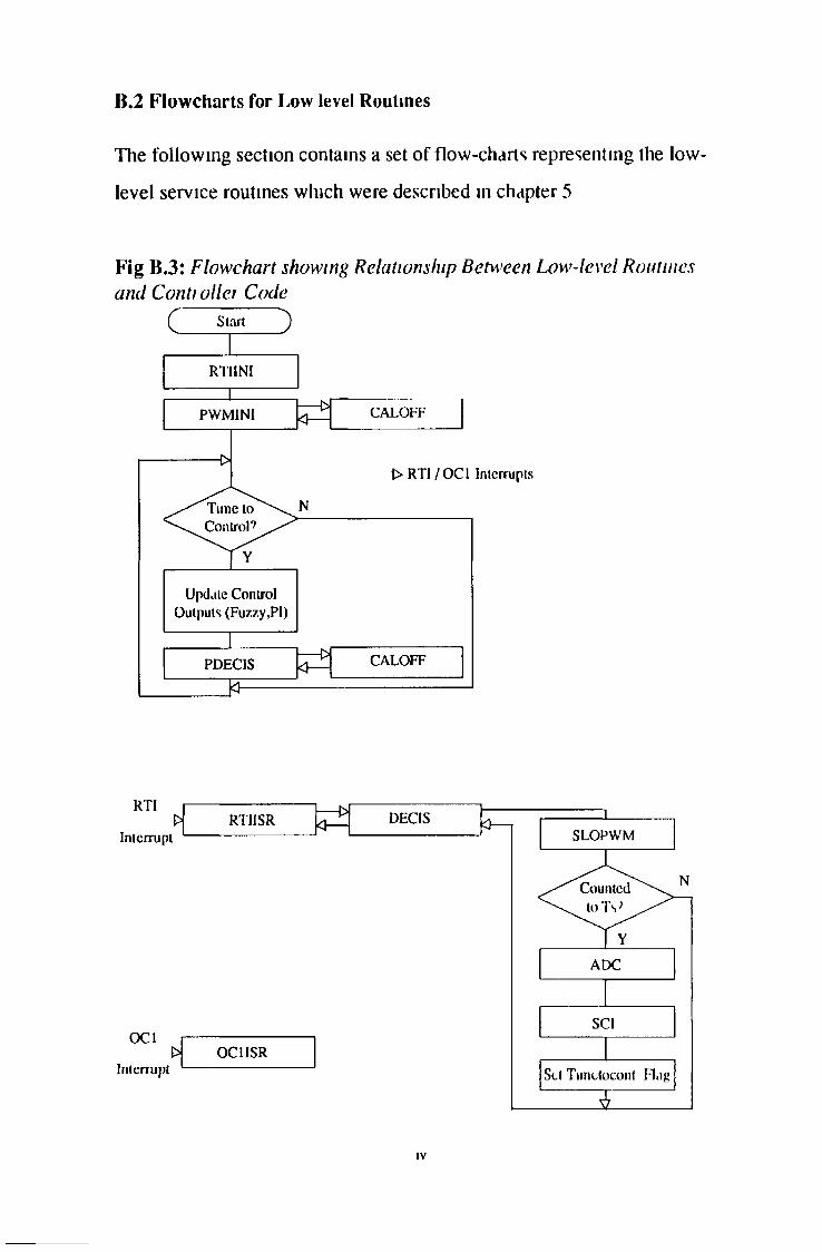
The following section contains a set of flow-charts representing the low- level service routines which were described in chapter 5

B.2 Flowcharts for Low level Routines

F ig B .3 : F l o w c h a r t s h o w i n g R e l a t i o n s h i p B e t w e e n L o w - l e v e l R o u t i n e s

a n d C o n t i o l l e i C o d e

IV

Fig B.4: Flowchart fo t Subi online RTIINI

V

Stari

Fig B.5: Flowchart fo r Subroutine DECIS

VI

Fig B,6: Flowchart fo r Subroutine ADC

VII

Start

Fig B.7: Flowchart fo r the Subioutine SCI

V III

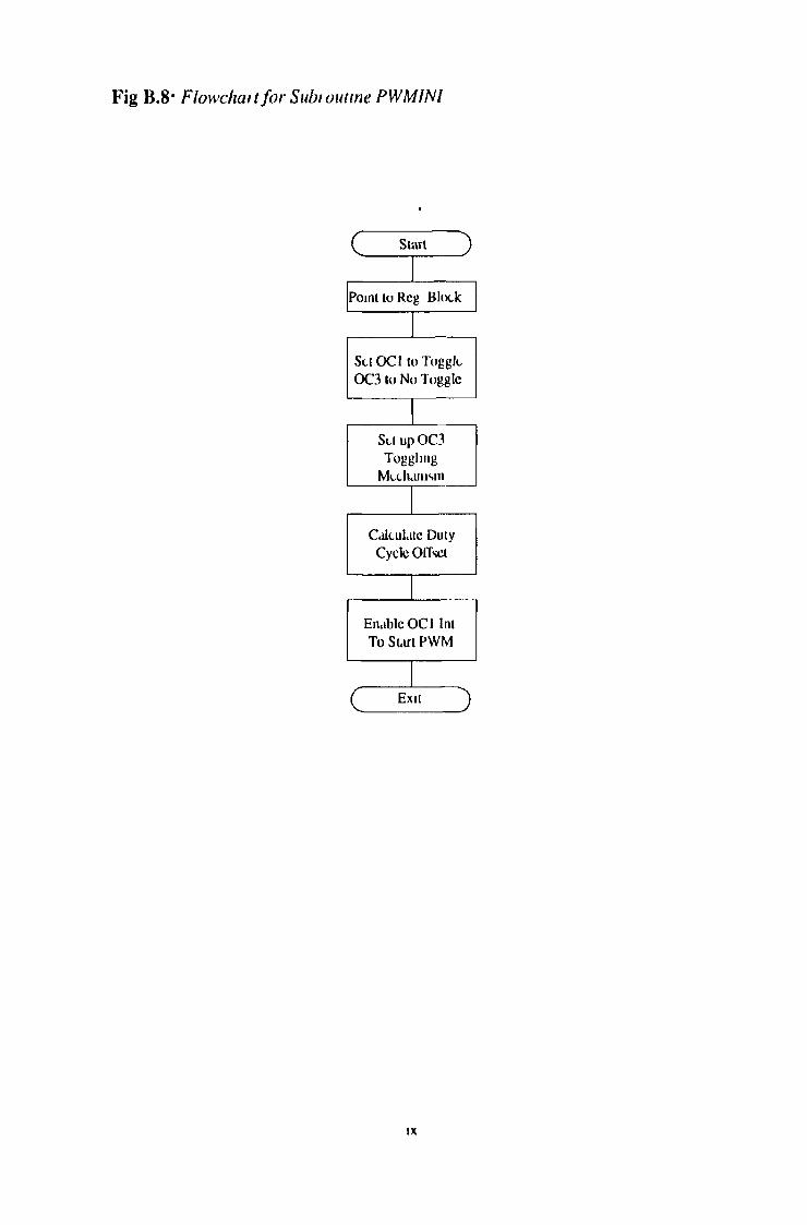
9

Fig B ,8# Flowchaìtfor Subi outine PWMINI

IX

\ t

Fig B.9 Flowchaitfor Subioutine PDECIS

Fig B.10: F l o w c h a r t f o i S u b i o u t i n e C A L O F F

X

Appendix C: Parameters used in Model of Cropping House

C.l : Variables in Model and Values of Parameters for OriginalModel

A Surface area o f cov er [/ 53 m2 jA Surface area o f trays [2 510~? m2 ]A Surface area o f water [w2]Cra Specific heat capacity o f air 0I0Jkg~!K~! JCn- Specific heat capacity o f water [4200Jkg~l K~l]e Current vapour pressure[mbat ]

Saturation vapour pressure[mbai ]E Evaporation from crop canopy [ kgs'1 ]h Current through heater [2 A]k , Leaf area index [6]Qv Volumetric flow rate o f air in a opping home [ msf t Heat lost tin ough conduction to outside [W]f t . Heat lost by convection [W]f t , Heat in by ventilation [¿F]f t „ V Heat out by ventilation [W]f t , Short - wave radiation flux inside [W]f t , Short - wave radiation flux outside [ W]

K CO2 induetoventilation^kgs_/]K v C02 out due to ventilation \kgs~! J

1

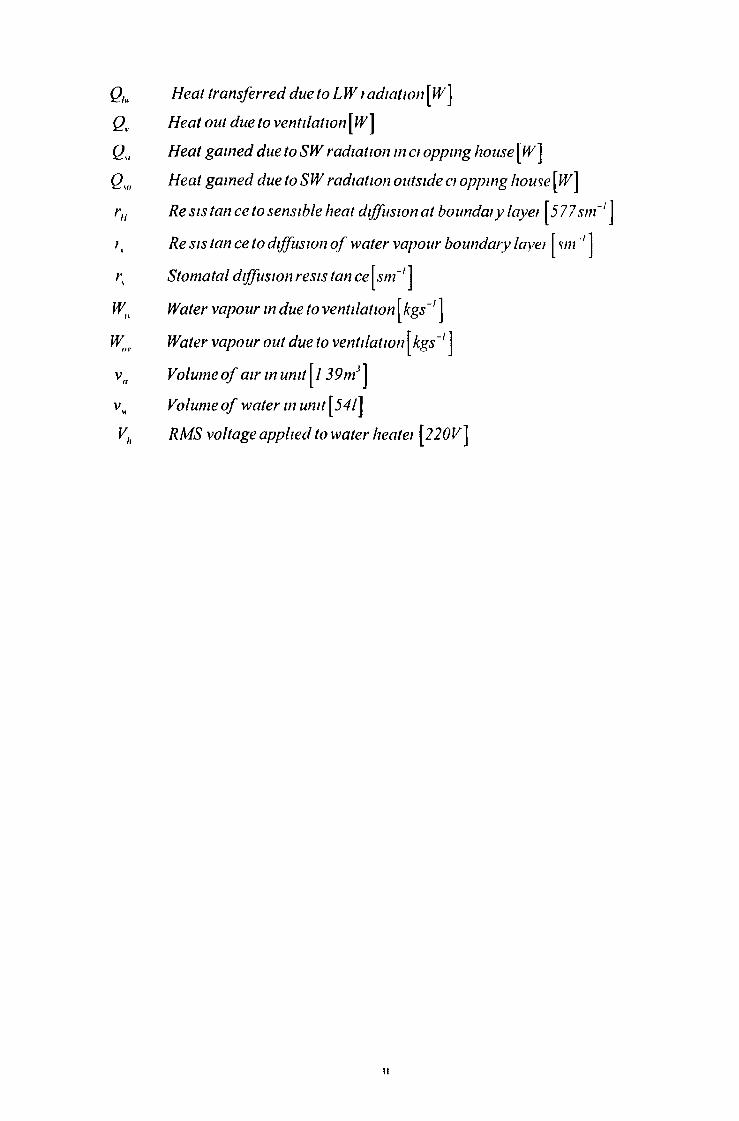
Qu Heat transferred due to LW? adiation [W]Qv Heat out due to ventilation [f'P]Qsl Heat gained due to SW radiation in a opping house [W]Qw Heat gained due to SW radiation outside a opping house [W]rH Re sis tan ce to sensible heat diffusion at boundary layer [5 77sin ! ji ( Re sis tan ce to diffusion o f water vapour boundary layer [ sin1 jrs Stomatal diffusion resis tan ce [s in 1 jWlx Water vapour in due to ventilation [kgs~l ]Wm Water vapour out due to ventilation[kgs~' ]va Volume o f air in umt^l 39 m3 jvM Volume o f water in unit[54l]Vh RMS voltage applied to water heater [220V]

u

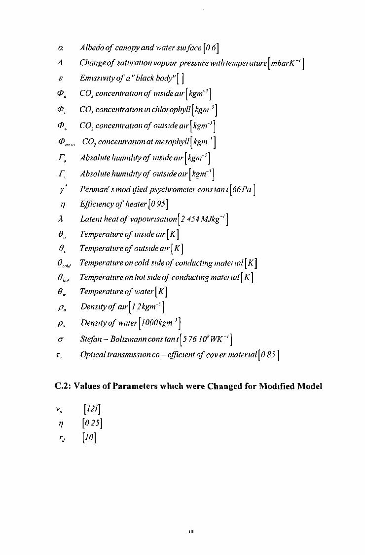
a Albedo o f canopy and water suiface \0 6\A Change o f saturation vapour pressure with tempei ature^m barK js Emissivity o f a " black body"[ ]0 a C02 concentration o f inside air^kgm~3 J0 C C02 concentration in chlorophyll [kgm~3 J0^ C 02 concentration o f outside air^kgin3 j0 mtw C02 concentration at mesophyll\kgm~' jr a Absolute humidity o f inside air^kgm"J]r t Absolute humidity o f outside air Jy* Penman* s mod ified psychrometet cons tan t [66Pa ]7; Efficiency o f heater \0 95]

X Latent heat o f vapourisation^ 454 MJkg~f ]6a Temperature o f inside air [K\0{ Temperature o f outside airOu)U{ Temperature on cold side o f conducting matei /«/ [AT]0fwt Temperature on hot side o f conducting mater /tf/[/C]0W Temperature o f water [A ]p a Density o f air\l 2kgm~3

Density o f water [ 1 OOOkgnf3 ] a Stefan - Boltzmann cons tan t^5 7610H WK ~4 ]r t Optical transmission co - efficient o f cov er material [0 85 ]

C.2: Values of Parameters which were Changed for Modified Model

V. [ « / ]1 [««]>1 ['»]

t t l

Appendix D: Extra Calculations

E l: Calculation of the Linear Approximation of the Rate of Net Long Wave Radiation Emissions from the Crop Canopy and Nutrient Surface.

The incident long wave radiation at the surface is given by

Qiw, = F(In Dlwhere 0O is the temperature of the surrounding air expressed in Kelvin and cris the Stefan-Boltzmann constant

The long wave radiation emitted by the crop canopy and nutrient solution surface can be expressed by

Qhvo = Eqn D2Where 0W is the temperature at the crop canopy and nutrient solution surface which is slightly greater than 6a and is also expressed in Kelvin

The temperature of the crop canopy and nutrient solution surface may be expressed as

0 W = 0 a + &0 Eqn D3where AO is the difference in temperature between the nutrient solution surface and the air inside the cropping house

The net heat loss from the crop canopy and nutrient solution surface is then

Q/w = o{0a + AO)4 - ae\ Eqn D4

By expanding this equation, we arrive at the following

Qlw = + 602aA02 + 4#aA03 + A04 ) Eqn D5

Since AO\ the difference between the two temperatures 0a and 0M, is typically inthe range 0°C -10°C, it is insignificant when compared to their absolute valueswhen expressed in Kelvin By ignoring the terms involving A£?2and higher orders we get

l

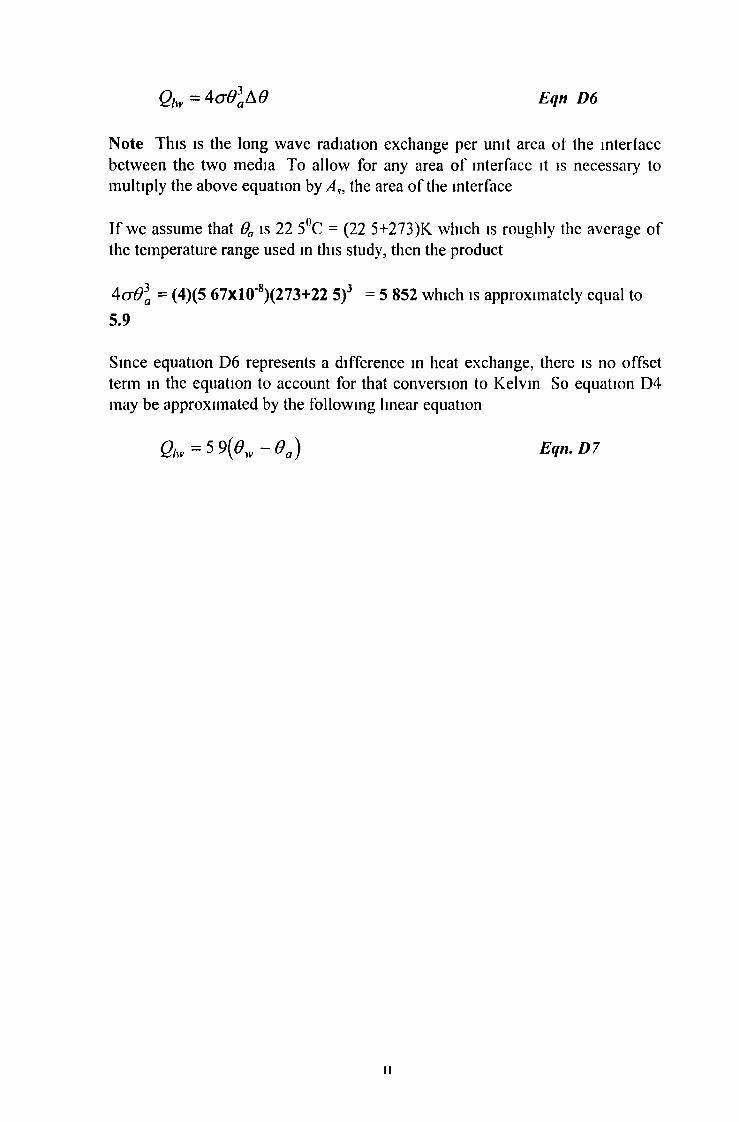
Qlw = 4a0l&e E q n D 6

Note This is the long wave radiation exchange per unit area of the interface between the two media To allow for any area o f interface it is necessary to multiply the above equation by the area o f the interface

I f we assume that 9a is 22 5°C = (22 5+273)K which is roughly the average o f the temperature range used in this study, then the product

4 ( j ^ = (4)(5 67x 10'8)(273+22 5)3 = 5 852 which is approximately equal to 5.9

Since equation D6 represents a difference in heat exchange, there is no offset term in the equation to account for that conversion to Kelvin So equation D4 may be approximated by the following linear equation

E q n . D 7

ii

Appendix E: References

Adams P 1980 “Nutrient Uptake by Cucumbers from Recirculating Solutions ’’Acta llo rticu ltu ra 98 ppl 19-126Astrom and W ittenm ark “Computer Controlled Systems” Prentice Hall First Edition 1984 Astrom and W ittenm ark “Computer Controlled Systems” Prentice Mall Second Edition 1990 Bailey B J “Designing fo r More Light and Less Energy” G rower July 19 1984 pp7,9,l I Bennett S “Real-time Computer Control” Prentice-Hall 1994Bernard J A , Asok R , K w a n K S , “Design and Experimental Evaluation o f a Fuzzy S) stem fo rthe Control o f Reactor Power” American Control Conference Vol 3 1985 ppl 466-1474Berry D & Berigan P “Interim Report on Vegetable Propagation Unit” Internal Report, DeptO f Control Systems and Electrical Engineering DIT Kevin StBerry D &Ryan M Final Report on the Vegetable Propagation Unit Forbairt 1995Bowman G E “Principles and Progress tn Environmental Control Systems1' Crop Processes inControlled Environments Vol 2 Academic Press 1972 pp63-76Control Sys & Electrical Eng DIT Kevin st Dublin 8 Dec 1993 9ppBurrage S W , Varlcy M J “Water Relations o f Lettuce Crown in Nutrient Film Culture”Actallorticiilturae Vol 98 1980, pp 79-86Busmger J A. “The Glasshouse/Greenhouse Climate “ In Physics of Plant Environment North Holland Publishing Co The Netherlands 1963Canham A “Coming to Terms with Tunnel Heating” Grow er Jul> 19 1984 pp26-27 Claudia G M , Gilberto H R , Guillermo P G “Low Cost Automatic Control Applied to an Experimental Greenhouse” 1992 IFAC Conference on Low Cost Automation (Components, Instrum ents, Applications) Pergammon 1993 pp313-316Cooper A , 1973 “Rapid Crop Turnaround is Possible with Experimental Nutrient film Technique” Grow er 79(18) pp!048,1050,1052Cooper A “Which side is Winning the Media War?” Grower Supplement (Tomatoes) 1983 3p Cox E "Fuzzy Fundamentals” IEEE Spectrum Oct 1992 p58Dexter A L “Introduction to Ftizzy Logic” Oxford International Summer Engineering Program m e July 1992Electric Council “Lighting tn Greenhouses” Growelectric Series 3rd Ed 1981Fisher J C Dept Control Sys and Electrical Eng DIT Kevin S t , Private Correspondence 1993Franklin & Powell “Feedback Control o f Dynamic S\ stems” Addison Wesley 1986 622ppGraves C “The Nutrient rd m Technique” Horticultural Reviews Vol 7 1985Grow er Publications “Commercial Applications o fN F T \ 1982 2nd Ed 96pHand D “The Promise o f Enrichment” Grower Supplement Vol 105 HN31,Jan 23 1986,4pHand D “Enrichment Needs Accurate Control and This is How you do i t” Grow er SupplementMay 1st 1986

i

H arris C J , Moore G , Brown M *'Intelligent Control Aspects o f Fuzzy Logic and Neural Nets ” W orld Scientific 1993,377 ppHayes R “The Development o f a Computer Simulation Model o f a Mushroom Growing Tunnel to Investigate Environmental Control” Prodceedmgs of the Symposium on Science and Cultivation of Edible Fungi Rotterdam 1991 pp307-313Hurd R and Graves C “Controlling the Water Supply” Grow er Vol 95 (19) Nov 1981 pp 17,19,21- 22Hurd R and Graves C “Soil Warming Needs Careful Control” G row er (17) July 19 1984 pp 15,17-19Jackson M B "Aeration in the Nutrient Film Technique o f Crop Production” Acta H o rtic u ltu re 1980 Vol 98 pp61-78Jenson M H and Collins W L “Hydroponic Vegetable Production” Horticultural Reviews Vol 5 1983 pp483-558Jones H G “Plants and Micro-climate” Cambridge University Press 1992 427ppKeen M "Cooling without Ventilation, an Israeli Breakthrough”, Grow er (114) July 12th 1990pp 14-15)Kindeian, M “Dynamic Modelling o f Greenhouse Environment” Transactions of the ASAE 1980 pp!232-1239Kuo B C “Digital Control Systems” HRW series in Electrical and Com puter Engineering 1980 Lee C C “Fuzzy Logic in Control Systems Fuzzy Logic Controller - Part I ” IEEE Transactions on Systems Man and Cybernetics 1990,Vol 20, No 2 pp 419 - 435Lee C C “Fuzzy Logic in Control Systems Fuzzy Logic Controller - Part 2 ” IEEE Transactions on Systems Man and Cybernetics 1990,Vol 20, No 2, pp404 - 417 Levine W “The Control Handbook ” CRC Press 1995Lyons G, “Defuzzification” W orkshop on Fuzzy Control DCU section D pp 1-20 1993MacConnell P F Sartorius C Owens D "Residential Environmental Regulation Using IntelligentFuzzy Control” IEE Colloquium Two Decades of Fuzzy Control, IEE Press, London 1993MacSiomain T Dept of Biology, DIT Kevin St Private Correspondence, Jan 1995M aher M J Teagasc Research Station, Kinsealy, Co Dublin, Private Correspondence, M arch1993Me Dowell T , Agripon Teo , Private Correspondence, Feb 1994M aher M J , H K Browne M J Mahon, R M Dunne and E W Ryan “Programme fo r Early Tomato Production” Internal Report Teagasc, Kinsealy Research Station 1993 M amdani F H “Fuzzy Control in Japan Learning Lessons” IFE Colloquium Two Decades of Fuzzy Control, IEE Press, London 1993M amdani E H , Assilian S “An Experiment m Linguistic Synthesis with a Fuzzy Logic Controller”, International Journal of Man Machine Studies, 1975 ,Vol 7, No l,ppl-13 Mathews R B , Saffell R A “Computer Control o f Humiditv m Experimental Greenhouses” Journal of Agricultural Engineering Research Vol 33 1986 pp2!3-221

n

M eath, F "Computer Simulation o f Mushroom Cropping Houses” MSc Thesis Dept Control Systems and Electrical Eng DIT Kevin St Dublin 8 1993M onteith J L "Principles o f Environmental Physics” Edward Arnold Contem porary Biology Series 1973 236ppMoorby J and Graves C J “The Effects o f Root and Air Temperature on the Growth o f Tomatoes” Acta H o rtic u ltu re 1980 98 29-43M orris, L G uThe theory o f fa n ventilation "A cta H o rt , 22, 1971 74-85M otorola INC “IICMOS Micro-Controller Unit Technical Data M anual” M C 68H C I1E9/D Rev 1 1991aM otorola “M 68H C II Reference M anual” MC68HC11RM/AD Rev 2 1991bM otorola “ Manual fo r 68H C II- based Fuzzy Engine and Editor” pp32 1993O ’ Flaherty T “Double Clad Polythene Greenhouses fo r Energy Saving” Farm and FoodResearch, M ount Salus Press Jan Feb 1977 pp l7 -!8Ogata “Discrete-time Control Systems” 1M Edition Prentice Hall 1987Procyk T , M amdani E H “A Linguistic S e lf Organising Controller” Automatica Vol 15 pp 15-30 1979Rosenberg N J , Blad B L ,Verma S B “Microclimate, the Biological E m ironm ent” Wiley 1983 Royle M , “The Case fo r Glass Double Glazing”, Grower 19th Ju lj 1984 pp 42-44,46 Schwartz D G , K hr G J ‘T tizzy Logic Flowers ut Japan” 1EFF Spectrum Inly 1992 pp 32-35 Self K “Designing with Fuzzy logic” IEEE Spectrum, Nov 1990 p42Seginer I, Levav N “Models as Tools in Greenhouse Climate Design ’’Agricultural Eng Dept Publication 115,Israel Institute of Technology Haifa Israel 1971 80ppStoutjesdijk P H and Barkmann J J “Micro-climate and Fauna” Opulus Press Sweden 1992pp88Tobi T , Hanafasu T “A Practical Application o f Fuzzy Control f o an Air-Conditioning System ” International Journal of Approximate Reasoning 1991 Vol 5 pp331-348Ud ink ten Cate "Modelling and Adaptive Control o f Greenhouse Climates” PhD Thesis Techmsche Hogcschool Twente 1983 pp 145Van Lmdmgham H “Introduction to Digital Control Systems” MacMillan London 1985 W insor G W “Progress in Nutrient Film Culture” Span 1980 23(1) pp7-9 W hite D C S “Heat Flow and D iffusion” in Biological Physics Chapm an &Hall 1974 W orld Book Science Year “Human Population Growth”, pp206-2251, 993Yeast Products ,Private correspondence Yeast Products Research Laboratory, Fmglas Dublin July 1994Young P, Private Correspondance Centre for Research in Environmental Systems, University of Lancaster 1994

in