Biogeosciences, 12, 5061–5074, 2015

www.biogeosciences.net/12/5061/2015/

doi:10.5194/bg-12-5061-2015

© Author(s) 2015. CC Attribution 3.0 License.

Environmental drivers of drought deciduous phenology in the

Community Land Model

K. M. Dahlin1,2, R. A. Fisher2, and P. J. Lawrence2

1Department of Geography, Michigan State University, East Lansing, Michigan, USA2Climate and Global Dynamics Division, National Center for Atmospheric Research, Boulder, Colorado, USA

Correspondence to: K. M. Dahlin (kdahlin@msu.edu)

Received: 6 March 2015 – Published in Biogeosciences Discuss.: 16 April 2015

Revised: 30 July 2015 – Accepted: 5 August 2015 – Published: 26 August 2015

Abstract. Seasonal changes in plant leaf area have a substan-

tial impact on global climate. The presence of leaves and the

time when they appear affect surface roughness and albedo,

and the gas exchange occurring between leaves and the atmo-

sphere affects carbon dioxide concentrations and the global

water system. Thus, correct predictions of plant phenological

processes are important for understanding the present and fu-

ture states of the Earth system. Here we compare plant phe-

nology as estimated in the Community Land Model (CLM)

to that derived from satellites in drought deciduous regions

of the world. We reveal a subtle but important issue in the

CLM: anomalous green-up during the dry season in many

semi-arid parts of the world owing to rapid upwards water

movement from wet to dry soil layers. We develop and im-

plement a solution for this problem by introducing an addi-

tional criterion of minimum cumulative rainfall to the leaf-

out trigger in the drought deciduous algorithm. We discuss

some of the broader ecological impacts of this change and

highlight some of the further steps that need to be taken to

fully incorporate this change into the CLM framework.

1 Introduction

Ecosystems change with the seasons in response to environ-

mental cues. Some of those cues are fixed, like day length,

while others are climate-driven and therefore vary from year

to year. The combination of fixed and climate-driven pheno-

logical cues poses an interesting problem in the face of cli-

mate change – climate-related drivers of phenology (temper-

ature and rainfall patterns) are likely to change (Lau et al.,

2013), while fixed cues will remain unchanged. Phenologi-

cal shifts due to climate change have already been identified

(e.g., Parmesan and Yohe, 2003). Phenology can refer to a

large number of patterns and behaviors in plants and animals

that shift with the seasons. Here, however, because we are fo-

cused on land surface model simulations, we use phenology

specifically to refer to intra-annual variations in leaf area in-

dex (LAI). Leaf area can vary significantly within a year and

is, therefore, a critical control on land–atmosphere feedbacks

(Lawrence et al., 2012).

Recent advances have greatly improved our ability to

predict seasonal patterns in northern temperate deciduous

forests (Richardson et al., 2012), but our understanding of

phenological patterns in stress or drought deciduous plants

(also called “raingreen”) remains weak (Guan et al., 2014;

Jenerette et al., 2010; Ma et al., 2013). The semi-arid ecosys-

tems that host the majority of drought deciduous woody

plants have relatively low biomass but make up a large frac-

tion of global land area (∼ 30 %; Scholes and Hall, 1996).

Their extensiveness alone makes them important to global

radiation budgets, but additionally these systems are likely

very sensitive to climate change given their apparent bista-

bility (Scholes and Hall, 1996; Staver et al., 2011). In semi-

arid ecosystems leaf-out is typically thought to be a function

of water availability (Reich, 1995; White et al., 1997); how-

ever, some woody plants leaf out several weeks before the

first rains of the season (Archibald and Scholes, 2007).

In an Earth system modeling context, the timing and mag-

nitude of plant phenology, and how these processes may

change, are critical for approximating the energy and car-

bon balances of the planet. Prognostic phenology has only

recently been incorporated into Earth system models, how-

ever, and its fidelity, particularly in semi-arid regions, re-

Published by Copernicus Publications on behalf of the European Geosciences Union.

5062 K. M. Dahlin et al.: Environmental drivers of drought deciduous phenology in the Community Land Model

mains poorly tested (Blyth et al., 2011; Lawrence et al., 2011;

Randerson et al., 2009). Lawrence et al. (2012) found that

the prognostic phenology in the Community Land Model

version 4 (CLM4(CN)) degraded estimates of latent heat

flux and other biophysical properties in comparison to using

prescribed, satellite-derived phenology (CLM4SP). Wang et

al. (2013) compared intra-annual variation in the fraction

of absorbed photosynthetically active radiation (fAPAR) in

CLM4CN to satellite-derived estimates and found substan-

tial differences in regional averages, zonal means, and inter-

annual trends. It is difficult, however, to isolate the impact

of the drought deciduous phenology algorithm using these

regional and zonal estimates.

Satellite-derived estimates of greenness, fAPAR, and LAI

have greatly improved our ability to study the environmental

drivers of phenology (Reed et al., 2009); however, the major-

ity of studies have focused on northern deciduous and boreal

forests (e.g., Delbart et al., 2006; White et al., 2009; Yang et

al., 2012). While fewer studies have focused on remote sens-

ing of phenology in semi-arid systems, Zhang et al. (2005)

found a strong relationship between greenness onset and the

start of the rainy season across the semi-arid parts of Africa.

They found a weaker relationship, however, between dor-

mancy and the end of rainy seasons, and they attribute this

weakness to differences in soil properties. Similarly, Ma et

al. (2013) found a strong relationship between greenness and

rainfall in northern Australia in both seasonal timing and

amplitude and Bradley et al. (2011) found a close relation-

ship between rainfall and seasonality in Amazonian savan-

nas. Interestingly, in Africa, Zhang et al. (2005) also showed

a strong relationship between latitude and both green-up and

dormancy onset, even in the narrow band of the Sahelian and

sub-Sahelian region, suggesting a possible link between phe-

nology and subtle changes in photoperiod at least in northern

Africa. Recently Guan et al. (2014) showed a relationship be-

tween woody plant cover and phenological timing in African

savannas.

In this study we address three questions related to the rep-

resentation of drought deciduous phenology in the CLM.

(1) How well does the CLM capture phenological patterns

of LAI among different drought deciduous plant functional

types (PFTs) as compared to satellite-derived estimates?; (2)

which parameters in the current version of the CLM have the

most leverage on drought deciduous phenology?; and (3) do

changes in the phenology algorithms in the CLM improve

the model’s representation of seasonal cycles regionally?

2 Methods

2.1 Model description

The CLM is the terrestrial component of the Community

Earth System Model (CESM; Lawrence et al., 2011); it sim-

ulates biogeophysical and biogeochemical processes includ-

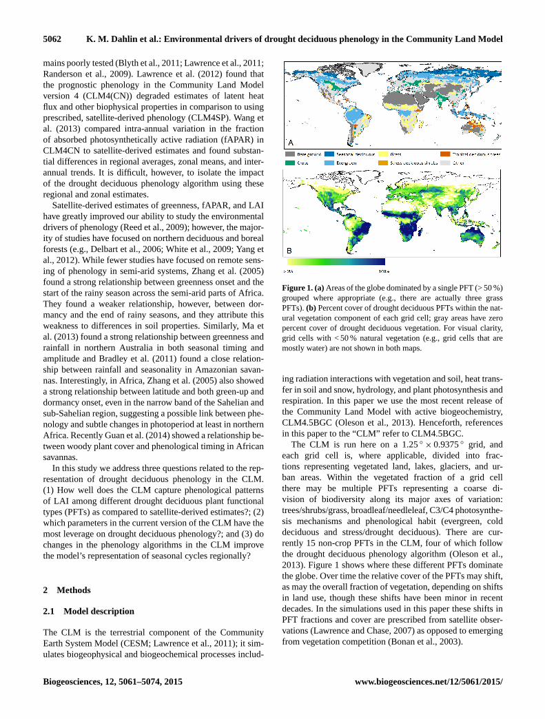
Figure 1. (a) Areas of the globe dominated by a single PFT (> 50 %)

grouped where appropriate (e.g., there are actually three grass

PFTs). (b) Percent cover of drought deciduous PFTs within the nat-

ural vegetation component of each grid cell; gray areas have zero

percent cover of drought deciduous vegetation. For visual clarity,

grid cells with < 50 % natural vegetation (e.g., grid cells that are

mostly water) are not shown in both maps.

ing radiation interactions with vegetation and soil, heat trans-

fer in soil and snow, hydrology, and plant photosynthesis and

respiration. In this paper we use the most recent release of

the Community Land Model with active biogeochemistry,

CLM4.5BGC (Oleson et al., 2013). Henceforth, references

in this paper to the “CLM” refer to CLM4.5BGC.

The CLM is run here on a 1.25 ◦× 0.9375 ◦ grid, and

each grid cell is, where applicable, divided into frac-

tions representing vegetated land, lakes, glaciers, and ur-

ban areas. Within the vegetated fraction of a grid cell

there may be multiple PFTs representing a coarse di-

vision of biodiversity along its major axes of variation:

trees/shrubs/grass, broadleaf/needleleaf, C3/C4 photosynthe-

sis mechanisms and phenological habit (evergreen, cold

deciduous and stress/drought deciduous). There are cur-

rently 15 non-crop PFTs in the CLM, four of which follow

the drought deciduous phenology algorithm (Oleson et al.,

2013). Figure 1 shows where these different PFTs dominate

the globe. Over time the relative cover of the PFTs may shift,

as may the overall fraction of vegetation, depending on shifts

in land use, though these shifts have been minor in recent

decades. In the simulations used in this paper these shifts in

PFT fractions and cover are prescribed from satellite obser-

vations (Lawrence and Chase, 2007) as opposed to emerging

from vegetation competition (Bonan et al., 2003).

Biogeosciences, 12, 5061–5074, 2015 www.biogeosciences.net/12/5061/2015/

K. M. Dahlin et al.: Environmental drivers of drought deciduous phenology in the Community Land Model 5063

Figure 2. Annual LAI cycles for LAI3g and CLM averaged for

1982–2010; shaded areas represent one standard deviation. Each

plot is averaged across a region as shown in Fig. 1. (a) Northern

Hemisphere (NH) C3 grasses; (b) NH C4 grasses; (c) Southern

Hemisphere (SH) C3 grasses; (d) SH C4 grasses; (e) Tropical de-

ciduous trees; (f) SH broadleaved deciduous shrubs.

In the CLM, drought deciduous plants are represented by

the “stress deciduous” phenology type, as distinct from the

evergreen or “seasonal” (cold) deciduous phenology types.

This designation allows for plants to lose their leaves via the

impact of cold, via the impact of drought, or via the onset of

short days, thus allowing the model to simulate, for exam-

ple, grass vegetation growing in an environment that is both

seasonally cold and seasonally dry. If the triggers for offset

are not reached in a given year, drought deciduous vegeta-

tion will follow the evergreen phenology algorithm, gaining

and losing fixed fractions of carbon with each time step. This

stress deciduous algorithm, described in more detail below

and in Oleson et al. (2013), was developed in part from White

et al. (1997), though that study was particularly focused on

grass phenology.

The deciduous algorithms are hierarchical, such that plants

classified as stress deciduous but growing at high latitudes

or in cold climates will follow the same onset/offset rules

as cold/seasonally deciduous plants. From the beginning of

a dormant period a “freezing day accumulator” is activated

whereby time steps with temperatures below freezing (0 ◦C)

are summed and if this sum exceeds 15 days then the plants

will follow both the winter deciduous and drought deciduous

algorithms. Leaf onset can only be triggered if day length is

greater than 6 h, a latitude-specific sum of growing degree

days has been reached (described in Oleson et al., 2013) and

the soil wetness criteria described below have been met.

In seasonally dry, warm regions (the focus of this paper)

where day length is never less than 6 h, leaf onset for the

stress deciduous phenology type is determined by soil wet-

ness. At the end of the previous offset period an accumulated

soil water index (SWI) is set to zero and accumulation is cal-

culated as

SWIn =

{SWIn−1

+ fday for ψsoil 3 ≥ ψthreshold

SWIn−1 for ψsoil 3 <ψthreshold, (1)

where n and n− 1 refer to the values in the previous and

current time steps, 9soil 3 is the soil water potential (MPa) in

the third soil layer (6.23–9.06 cm), 9threshold is −2 MPa, and

fday is a time step (30 min in CLM) as a fraction of a day.

Onset is triggered when SWI exceeds 15 days.

The rate of leaf onset (fraction of onset per time step),

which in the CLM is represented as the transfer of C and N

from a storage pool to the “display” leaf pool, is determined

by the number of days prescribed for onset, fixed at 30 days.

The rate (ronset) at each time step is defined as

ronset =

2

tonset

for tonset 6=1t

1

1tfor tonset = 1t

, (2)

where tonset is time remaining in the current onset period in

seconds and1t is the length of a time step (1800 s). The flux

of C out of the storage pool is then defined as the amount

in the C storage pool at that time step multiplied by ronset.

These functions result in a linearly decreasing flux out of the

transfer pool, so the rate of increase in LAI over the onset

period steadily decreases as C moves from the storage pool

to the display pool (see Fig. 14.1 in Oleson et al., 2013).

During the onset period, C and N are also transferred from

storage pools for fine roots, live and dead stems, and live

and dead coarse roots into these components’ respective dis-

played growth pools. During the growing season, C and N

taken up by the plant are accumulated in transfer pools, to be

used in the next growing season.

As long as the leaf onset period is complete, leaf offset

can be triggered by short (< 6 h) day length, a period of cold

temperatures (described in Oleson et al., 2013) or if the soil

dryness criteria described below has been met.

The offset soil wetness index (OSWI) can potentially start

accumulating time steps once the previous leaf onset phase

is complete. The algorithm differs slightly from the onset

trigger in that OSWI can increase or decrease as described

below.

OSWIn =

{OSWIn−1

+ fday for ψsoil 3 ≤ ψthreshold

max(OSWIn−1− fday, 0) for ψsoil 3 > ψthreshold

. (3)

where 9threshold is −2 MPa, and leaf offset is triggered when

OSWI equals 15 days.

Similar to the rate of leaf onset, leaf offset rate is a function

of the amount of time left in the offset period, fixed at 15

days:

roffset =21t

t2offset

(4)

Carbon fluxes into the litter pool are only calculated for

leaves and fine roots (stems and coarse roots cannot shrink).

Nitrogen fluxes into the litter pool reflect retranslocation of

N prior to offset. See Oleson et al. (2013) for more details.

The model runs used in the global simulations described

here ran for 45 years, and were started from an equilib-

rium baseline state generated by a standard CLM spin-up

www.biogeosciences.net/12/5061/2015/ Biogeosciences, 12, 5061–5074, 2015

5064 K. M. Dahlin et al.: Environmental drivers of drought deciduous phenology in the Community Land Model

Figure 3. Seasonal cycles of rainfall (mm day−1, gray bars), leaf area index (LAI, green lines and black dots) and soil water potential in the

third layer (MPa, blue lines) in CLM and CLM-MOD for 1 year (2001).

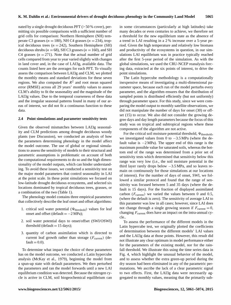
Figure 4. Illustration of Latin hypercube (LH) variable exploration

analysis results – here each line represents one simulation from 1

year of the LH analysis without the additional rainfall trigger. Each

line is from a model run with slightly different values for the vari-

ables considered. In actuality 100 simulations were performed, but

for visual clarity we are showing a selection of 10 simulations.

run (as described in detail by Koven et al., 2013) cycling

meteorological conditions of 1948–1972. The present-day

run (1965–2010) used CRU-NCEP meteorological reanaly-

sis data (Vivoy, 2012) and transient CO2 concentrations to

drive the model. Soil type and land cover are prescribed in

the model, and recent work has suggested that the soil resis-

tance parameterization may be unrealistic in arid ecosystems

(Swenson and Lawrence, 2014). More details on CLM are

available in Oleson et al. (2013).

2.2 Satellite-derived LAI

We compared the model-derived estimates of LAI to those

estimated from the Advanced Very High Resolution Ra-

diometer sensors (AVHRR) onboard NOAA satellites. These

data are available twice per month and span 1981 to 2011.

They are supplied at 1/12 ◦ resolution. A detailed description

of the development of the LAI product (hereafter LAI3g) is

in Zhu et al. (2013).

To ensure the most appropriate comparison possible, the

LAI3g data set was rescaled to match the mean monthly LAI

output from the CLM. First, the two LAI3g maps generated

for each month were averaged, and then the LAI3g pixels

were aggregated (averaged) to match the size of a CLM grid

cell (∼ 165 pixels per grid cell). If more than 80 % of the

grid cell did not have values in LAI3g (mostly applicable at

high latitudes), the entire grid cell was removed from further

analysis. Finally, the aggregated LAI3g data was resampled

using a nearest neighbor approach to align with the CLM grid

for further analysis. All spatial and statistical analyses were

performed in R (R Core Team, 2013) using the ncdf (Pierce,

2011), raster (Hijmans and van Etten, 2013) and rgdal (Bi-

vand et al., 2013) packages.

2.3 Comparing LAI3g to CLM LAI

We first compared LAI3g to the CLM output for 1982 (the

first full year of LAI3g) to 2010 (the last available year of

the CRU-NCEP forcing data set for CLM), aggregating val-

ues by zones based on dominant PFT and hemisphere. To ag-

gregate into PFT classes, we only considered grid cells domi-

Biogeosciences, 12, 5061–5074, 2015 www.biogeosciences.net/12/5061/2015/

K. M. Dahlin et al.: Environmental drivers of drought deciduous phenology in the Community Land Model 5065

nated by a single drought deciduous PFT (> 50 % cover), per-

mitting six possible comparisons with a sufficient number of

grid cells for comparison: Northern Hemisphere (NH) tem-

perate C3 grasses (n= 180), NH C4 grasses (n= 234), trop-

ical deciduous trees (n= 242), Southern Hemisphere (SH)

deciduous shrubs (n= 68), SH C3 grasses (n= 160), and SH

C4 grasses (n= 271). Note that the actual number of grid

cells compared from year to year varied slightly with changes

in land cover and, in the case of LAI3g, available data. The

counts listed here are the averages for each PFT. To visually

assess the comparison between LAI3g and CLM, we plotted

the monthly means and standard deviations for these seven

regions. We also computed the R2 and root mean squared

error (RMSE) across all 29 years’ monthly values to assess

CLM’s ability to fit the seasonality and the magnitude of the

LAI3g values. Due to the temporal coarseness of these data

and the irregular seasonal patterns found in many of our ar-

eas of interest, we did not fit a continuous function to these

data.

2.4 Point simulations and parameter sensitivity tests

Given the observed mismatches between LAI3g seasonal-

ity and CLM predictions among drought deciduous woody

plants (see Discussion), we conducted an analysis of how

the parameters determining phenology in the model affect

the model outcome. The use of global or regional simula-

tions to assess the sensitivity of models to their structural and

parametric assumptions is problematic on account of both

the computational requirements to do so and the high dimen-

sionality of the model outputs, which can hinder understand-

ing. To avoid these issues, we conducted a sensitivity test on

the major model parameters that control seasonality in LAI

at the point scale. In these point simulations we focused on

low-latitude drought deciduous ecosystems, and selected six

locations dominated by tropical deciduous trees, grasses, or

a combination of the two (Table 1).

The phenology model contains three empirical parameters

that collectively describe the leaf onset and offset algorithms:

1. critical soil water potential (9threshold) values for leaf

onset and offset (default=−2 MPa);

2. soil water potential days to onset/offset (SWI/OSWI)

threshold (default= 15 days);

3. quantity of carbon assimilation which is directed to

current leaf growth rather than storage (Fcurrent) (de-

fault= 0.0).

To determine what impact the choice of these parameters

has on the model outcome, we conducted a Latin hypercube

analysis (McKay et al., 1979), beginning the model from

a spun-up state with default parameters. We then perturbed

the parameters and ran the model forwards until a new LAI

equilibrium condition was detected. Because the nitrogen cy-

cle is active in CLM, soil biogeochemical equilibrium can

in some circumstances (particularly at high latitudes) take

many decades or even centuries to achieve, we therefore set

a threshold for the new equilibrium state as the absence of

a trend in LAI resulting in a 2 % increase over a 5-year pe-

riod. Given the high temperature and relatively low biomass

and productivity of the ecosystems in question, in our sim-

ulations LAI equilibrium was in practice typically reached

after the first 5-year period of the simulation. As with the

global simulations, we used the CRU-NCEP reanalysis forc-

ing data, extracted at the six points of interest, to drive the

point simulations.

The Latin hypercube methodology is a computationally

inexpensive means of investigating a multi-dimensional pa-

rameter space, because each run of the model perturbs every

parameter, and the algorithm ensures that the distribution of

sampled points is distributed efficiently (but not uniformly)

through parameter space. For this study, since we were com-

paring the model output to monthly satellite observations, we

did not manipulate the number of days for onset (30) or off-

set (15) to occur. We also did not consider the growing de-

gree days and day length parameters because the focus of this

study was on tropical and subtropical regions where these

components of the algorithm are not active.

For the critical soil moisture potential threshold,9threshold,

we investigated values from 0 to −3.5 MPa (where the de-

fault value is −2 MPa). The upper end of this range is the

maximum possible value for saturated soils, whereas the bot-

tom end of the range was determined from a prior set of

sensitivity tests which determined that sensitivity below this

range was very low (i.e., the soil moisture potential in the

third layer rarely drops below −3.5 MPa, and so leaves re-

main on continuously for those simulations at our locations

of interest). For the number of days of onset, SWI, we fol-

lowed a similar protocol and found that the range of sen-

sitivity was focused between 5 and 35 days (where the de-

fault is 15 days). For the fraction of displayed assimilated

carbon (Fcurrent) we varied the values between 0 and 0.5,

(where the default is zero). The sensitivity of average LAI to

this parameter was low in all cases; however, since LAI does

not change through a single growing season if Fcurrent = 0,

changing Fcurrent does have an impact on the intra-annual cy-

cle..

To assess the performance of the different models in the

Latin hypercube test, we originally plotted the coefficients

of determination between the different models’ LAI values

and the LAI3g data at those points. However, this result did

not illustrate any clear optimum in model performance either

for the parameters of the existing model, nor for the rain-

fall threshold. We illustrate this using the time series data in

Fig. 4, which highlight the unusual behavior of the model,

and to assess whether the extra green-up period during the

dry season had been eliminated in any of the parametric per-

mutations. We ascribe the lack of a clear parametric signal

to two effects. First, the LAI3g data were necessarily ag-

gregated to monthly values, meaning that the primarily sub-

www.biogeosciences.net/12/5061/2015/ Biogeosciences, 12, 5061–5074, 2015

5066 K. M. Dahlin et al.: Environmental drivers of drought deciduous phenology in the Community Land Model

Table 1. List of locations for point simulations and percent cover of plant functional types (PFTs). PFTs with no coverage at any point are

not listed.

Point.name Latitude Longitude Bare Broadleaf Broadleaf Broadleaf C3 C4 Crops

ground Evergreen Evergreen Deciduous Grasses Grasses

Tree Tropical Tree Temperate Tree Tropical

Brasilia −15 −51 0.46 1.69 0 16.52 8.83 62.35 10.15

Western Brazil −6 −39 2.66 0 0 35.4 9.04 40.6 12.3

South Chad 11 18 1.34 0 0 34.26 0.03 60.22 4.16

Eastern Zambia −13 32 0.22 0.56 1.27 26.4 37.81 26.39 7.35

South Ethiopia 5.5 40 8.75 0.13 0.02 63.1 19.12 5.42 3.47

Darwin Australia −15 130.5 15.94 0 0 35.73 0 48.33 0

monthly variation between ensemble members was masked.

Second, the timing of the secondary leaf-on period in the dry

season was the emergent property of the oscillatory (and thus

somewhat chaotic) dynamics of the soil–vegetation feedback

on soil moisture. We thus conclude that the model deficiency

is caused by structural, not parametric, issues.

Once we determined that we could not eliminate the dry

season green-up by changing the existing model parameters,

we considered four possible additions to the model. The first

three are described here but, for brevity, are not quantified

in the results. First, we considered that using the third soil

layer in CLM may be an arbitrary choice of soil depth, and

that usage of the soil moisture potential derived drought in-

dex (“BTRAN”, Oleson et al., 2013), which is weighted by

vertical root fraction across the whole rooting depth profile,

might provide a more physiologically relevant metric and be

less prone to increases due to upwards moisture diffusion in

the dry season. However, since the exponential root profile in

the CLM weights the top soil layers (including layer 3) more

strongly than the lower layers with fewer roots, this metric

was just as prone to increasing water potential during the dry

season as soil water potential in the third soil layer.

Second, we implemented leaf onset as a function of a total

column soil moisture content threshold rather than soil mois-

ture potential. We postulated that the redistribution of water

causes the erroneous behavior and that this would not impact

total column moisture. However, the establishment of a sin-

gle global threshold for total soil moisture is challenging as a

number of different variables impact soil moisture, including

the variation in soil water retention capacities between dif-

ferent land points, and by the interaction between leaf area,

evaporation rate and deep soil moisture content. Variation in

rainfall and evaporation rates affects the equilibrium water

content of deep soils, which changes the total column soil

moisture content between locations and years, but not the

physiologically relevant upper soil moisture potential. There-

fore, we abandoned this possible driver of drought deciduous

phenology.

Third, we considered a metric of triggering leaf flush by

the rate of change of total column soil moisture, rather than

soil moisture potential. However, this methodology also gen-

erates erroneous behavior, on account of the ability of the

CLM hydrology model to extract water from the water table

or aquifer along a water potential gradient. Thus, when water

potential is low in the bottom soil layer in the dry season, the

rate of change of total soil moisture can be positive without

any input from rainfall.

2.5 Rainfall model

To correct biases uncovered in the model output (described

below) we introduced a simple trigger into the model, that

time-averaged 10-day precipitation must exceed a given

threshold before leaf onset is triggered. This approach re-

quires the addition of a new parameter, rain_threshold, into

the model, which is the threshold over which the sum of

precipitation over 10 days must be for leaf-on to occur.

Leaf onset is thus triggered if 10-day rain is higher than

rain_threshold and if the SWI is greater than 15 days.

We then used a Latin hypercube approach again to deter-

mine the sensitivity of the model to rain_threshold at our six

chosen geographical points. We considered a range of rain-

fall rates, requiring that it rain 20 mm over the course of 5 to

60 days in order for plants to begin growing leaves. To test

the global impact of these parameter changes, we ran CLM

with the new rainfall-based trigger and compared the results

both at several points and globally.

2.6 Global simulations

We used a number of different metrics to globally compare

CLM to the LAI3g data and, later, to the modified version of

the model (CLM-MOD). First we compared maps of max-

imum annual LAI and differences between the three maps.

We also developed an algorithm to count the number of LAI

peaks per year in all three data sets on grid cells with an LAI

range greater than 1 by counting the number of times per

year that the difference between one month’s LAI and the

next was negative, then taking the mode across all 29 years.

Finally, we calculated the coefficient of determination (R2)

in each grid cell, comparing the monthly LAI3g data to CLM

and CLM-MOD to identify areas with strong agreement be-

Biogeosciences, 12, 5061–5074, 2015 www.biogeosciences.net/12/5061/2015/

K. M. Dahlin et al.: Environmental drivers of drought deciduous phenology in the Community Land Model 5067

tween the remotely sensed data and the models, and areas

with weak relationships.

The recent focus on land model benchmarking has led to

a number of additional suggested methods for assessing sea-

sonality in models compared to data (e.g., Randerson et al.,

2009; Kelley et al., 2013); however, none of the proposed

metrics would have captured the central issue addressed in

this paper – model output with two or more peaks per year,

data with only one – as they begin with the unstated assump-

tion that seasonality is unimodal over the course of a year,

as do measures of the start and end of the growing season. In

Randerson et al. (2009) seasonality is assessed by identifying

the month of peak LAI and comparing that to MODIS LAI

(MOD15A2), and in Kelley et al. (2013) several, more com-

plicated metrics are introduced (Eqs. 7–9) to again produce

single numbers to compare a model’s seasonality to a bench-

mark data set. In these examples, as in other benchmarking

studies, the focus is on producing a single number, which,

while useful, can miss important details.

3 Results

3.1 Seasonal patterns in CLM

We found generally good agreement between LAI3g and

CLM averaged across grass-dominated regions. In a compar-

ison of monthly values from 1982 to 2010 for the single PFT

dominated regions in Fig. 1, R2 values ranged from 0.54 to

0.9 (Table 2) with the majority of the grass R2 values greater

than 0.7. Figure 2 shows the monthly values across all years,

and we see similar results – generally good correspondence,

especially in seasonal pattern, between LAI3g and the CLM

runs in the grass-dominated regions. The root mean squared

error (RMSE) values in Table 2 and Fig. 2b and c show that

CLM does not always capture the appropriate LAI values in

grasslands, but the seasonal cycle is reasonably correct.

In contrast, CLM does not successfully capture phenolog-

ical patterns or values in areas dominated by woody drought

deciduous vegetation. Among tropical deciduous trees CLM-

predicted LAI appears to be both too high and out of phase

with the satellite observations (Fig. 2e) while CLM shows no

apparent seasonality among deciduous shrubs in the South-

ern Hemisphere (Fig. 2f), while LAI3g shows a slight cycle

ranging from 0.4 to 0.7 LAI.

3.2 Point simulations and sensitivity tests

To look more closely at seasonal patterns in drought decidu-

ous locations, we selected six points around the globe across

a range of latitudes dominated by a mixture of broadleaf de-

ciduous tropical trees, and C3 and C4 grasses (Table 1), all

of which use the same stress deciduous phenology algorithm.

To better understand the phenological patterns, we re-ran

CLM using the same methods as described above but record-

ing daily outputs of relevant parameters including LAI, soil

water potential, rainfall, and others. Plots of the seasonal cy-

cles at these specific points using daily model output (solid

green lines in Fig. 3) revealed a pattern whereby CLM ap-

pears to put leaves on during the “brown season” in the

LAI3g data in some of the points in addition to during the

LAI3g green season. We note, however, that some areas in

reality do have two separate growing seasons per year (e.g.,

Fig. 3e). Despite the lack of rainfall, soil water potential in

the third soil layer in CLM rises during the dry season and is

extremely variable in the dry season, on account of periods

of high transpiration when plants leaf out (blue dot-dashed

line in Fig. 3).

We used the output from the Latin hypercube approach at

these six points to vary the parameters of interest (days to on-

set/offset, critical soil water potential, carbon assimilation) to

assess whether modification of parameter values could ame-

liorate the problem of plants leafing out during the dry season

in CLM. We found, however, that simply varying the param-

eters of the existing model within the parameter space inves-

tigated (and assuming no large nonlinearities in the model

response surface) did not remove the dry season leaf-out in

the model (Fig. 4).

In order to address this issue, we considered a number of

structural perturbations to the leaf-on and leaf-off algorithms

(described in the discussion below), but ultimately decided

on adding a new parameter, rain_threshold, to the model. We

then used the same Latin hypercube approach to determine

the best fitting values for this parameter (Fig. 5). This addi-

tional leaf-on criterion, set so that 20 mm of rain must ac-

cumulate over 10 days in order for leaf onset to occur, led

to a removal of the brown season leaf-out in CLM (dashed

green line in Fig. 3) without preventing two green seasons

per year, as is possible in some semi-arid regions (e.g., parts

of Ethiopia, Fig. 3e). While this new rainfall threshold im-

proved model performance both at our points and globally

(see below), we note that the model did not appear to be par-

ticularly sensitive to the amount of rain that fell, as long as

some rain did fall, but this threshold, and the drought de-

ciduous algorithm as a whole, deserves more research into

seasonal drivers.

3.3 Global simulations

To test how well the additional rainfall parameter performed

globally, we ran CLM with the new rainfall parameter for 45

years (CLM-MOD) from the same equilibrium baseline state

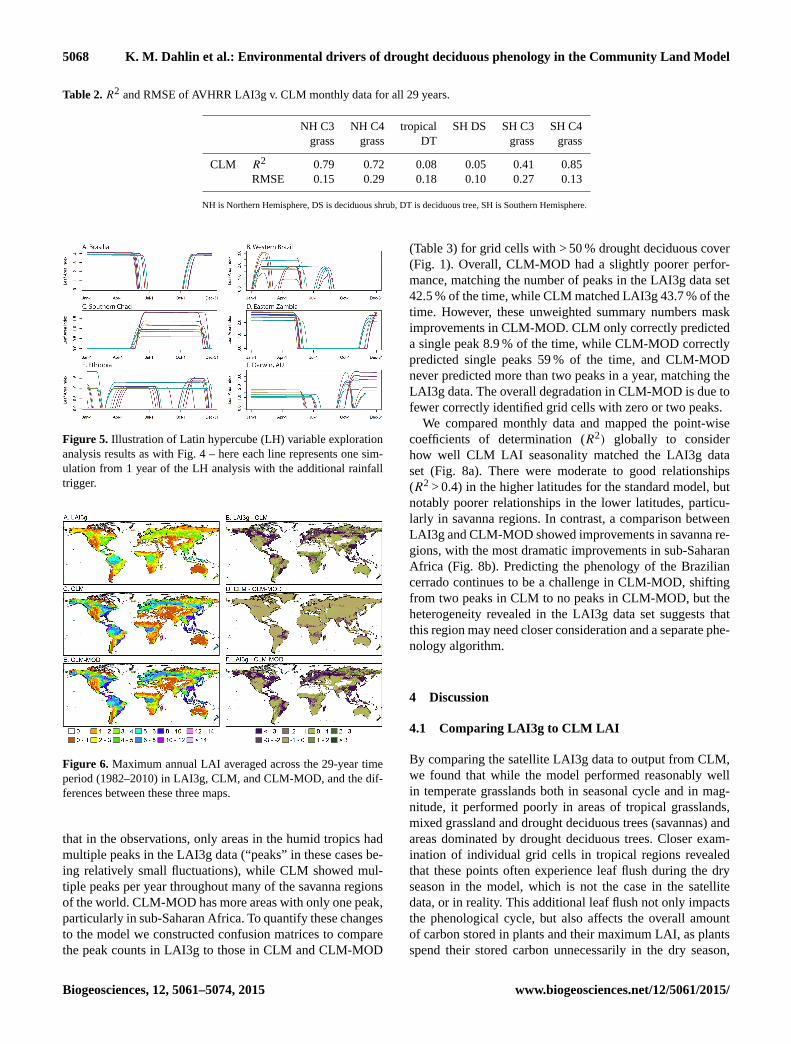
as was used in the first run described. Measures of maximum

LAI (Fig. 6) and mean LAI (data not shown) in CLM-MOD

showed closer matches to LAI3g than CLM. While CLM val-

ues remain far too high in the evergreen tropics, the maxi-

mum LAI values in deciduous savanna regions did increase

appropriately in CLM-MOD to better match the LAI3g data.

To test whether the poor fit between CLM and LAI3g was

due to multiple annual LAI peaks in CLM we counted the

number of peaks per year in each data set (Fig. 7). We found

www.biogeosciences.net/12/5061/2015/ Biogeosciences, 12, 5061–5074, 2015

5068 K. M. Dahlin et al.: Environmental drivers of drought deciduous phenology in the Community Land Model

Table 2. R2 and RMSE of AVHRR LAI3g v. CLM monthly data for all 29 years.

NH C3 NH C4 tropical SH DS SH C3 SH C4

grass grass DT grass grass

CLM R2 0.79 0.72 0.08 0.05 0.41 0.85

RMSE 0.15 0.29 0.18 0.10 0.27 0.13

NH is Northern Hemisphere, DS is deciduous shrub, DT is deciduous tree, SH is Southern Hemisphere.

Figure 5. Illustration of Latin hypercube (LH) variable exploration

analysis results as with Fig. 4 – here each line represents one sim-

ulation from 1 year of the LH analysis with the additional rainfall

trigger.

Figure 6. Maximum annual LAI averaged across the 29-year time

period (1982–2010) in LAI3g, CLM, and CLM-MOD, and the dif-

ferences between these three maps.

that in the observations, only areas in the humid tropics had

multiple peaks in the LAI3g data (“peaks” in these cases be-

ing relatively small fluctuations), while CLM showed mul-

tiple peaks per year throughout many of the savanna regions

of the world. CLM-MOD has more areas with only one peak,

particularly in sub-Saharan Africa. To quantify these changes

to the model we constructed confusion matrices to compare

the peak counts in LAI3g to those in CLM and CLM-MOD

(Table 3) for grid cells with > 50 % drought deciduous cover

(Fig. 1). Overall, CLM-MOD had a slightly poorer perfor-

mance, matching the number of peaks in the LAI3g data set

42.5 % of the time, while CLM matched LAI3g 43.7 % of the

time. However, these unweighted summary numbers mask

improvements in CLM-MOD. CLM only correctly predicted

a single peak 8.9 % of the time, while CLM-MOD correctly

predicted single peaks 59 % of the time, and CLM-MOD

never predicted more than two peaks in a year, matching the

LAI3g data. The overall degradation in CLM-MOD is due to

fewer correctly identified grid cells with zero or two peaks.

We compared monthly data and mapped the point-wise

coefficients of determination (R2) globally to consider

how well CLM LAI seasonality matched the LAI3g data

set (Fig. 8a). There were moderate to good relationships

(R2 > 0.4) in the higher latitudes for the standard model, but

notably poorer relationships in the lower latitudes, particu-

larly in savanna regions. In contrast, a comparison between

LAI3g and CLM-MOD showed improvements in savanna re-

gions, with the most dramatic improvements in sub-Saharan

Africa (Fig. 8b). Predicting the phenology of the Brazilian

cerrado continues to be a challenge in CLM-MOD, shifting

from two peaks in CLM to no peaks in CLM-MOD, but the

heterogeneity revealed in the LAI3g data set suggests that

this region may need closer consideration and a separate phe-

nology algorithm.

4 Discussion

4.1 Comparing LAI3g to CLM LAI

By comparing the satellite LAI3g data to output from CLM,

we found that while the model performed reasonably well

in temperate grasslands both in seasonal cycle and in mag-

nitude, it performed poorly in areas of tropical grasslands,

mixed grassland and drought deciduous trees (savannas) and

areas dominated by drought deciduous trees. Closer exam-

ination of individual grid cells in tropical regions revealed

that these points often experience leaf flush during the dry

season in the model, which is not the case in the satellite

data, or in reality. This additional leaf flush not only impacts

the phenological cycle, but also affects the overall amount

of carbon stored in plants and their maximum LAI, as plants

spend their stored carbon unnecessarily in the dry season,

Biogeosciences, 12, 5061–5074, 2015 www.biogeosciences.net/12/5061/2015/

K. M. Dahlin et al.: Environmental drivers of drought deciduous phenology in the Community Land Model 5069

Table 3. Confusion matrices comparing grid cell peak counts between LAI3g and the two model data sets. “%” rows and columns are the

percent of the correct values (diagonal) compared to the sums for the respective rows and columns. n/a is not applicable.

A. LAI3g vs. CLM B. LAI3g vs. CLM-MOD

LAI3g LAI3g

0 1 2 > 2 % 0 1 2 > 2 %

CLM

0 436 164 145 0 58.5

CLM-MOD

0 365 279 277 0 39.6

1 28 74 130 0 31.9 1 242 439 407 0 43.2

2 196 555 499 0 39.9 2 60 63 125 0 50.4

> 2 7 42 35 0 0 > 2 0 0 0 0 n/a

% 65.4 8.9 61.7 n/a 43.7 % 54.7 59.0 15.5 n/a 42.5

Figure 7. Mode of annual peak count analysis for the three simula-

tions. (a) LAI3g; (b) CLM; (c) CLM-MOD.

leaving less carbon available during the wet season for grow-

ing leaves. This addition of leaf carbon in the dry season also

may affect the fire cycle in varying ways around the dry trop-

ics. While these runs of the model were not coupled to a dy-

namic atmosphere, we expect that this dry season leaf flush

could also impact the climate, potentially having an unrealis-

tic cooling effect by moving more water into the atmosphere

during what should be a very dry time of year, but also dark-

ening the land surface, possibly leading to a slight warming.

Figure 8. Coefficients of determination (R2) between LAI3g and

the two model versions.

The mechanism behind the dry season leaf flush is an

increase in soil water potential in the dry season to levels

above the prescribed leaf-out threshold. These increases de-

rive from the assumption in CLM that all of the land surface

sits on top of an unconfined aquifer. In most cases this aquifer

is either irrelevant because plenty of soil water is available or

it is essential to plant survival in areas where aquifers do ex-

ist in the real world. In semi-arid systems, however, this ex-

tra pool of soil water becomes problematic in the dry season.

The top soil layers dry out due to soil evaporation and, when

plants are active, evapotranspiration, establishing a water po-

tential gradient which causes water to be transferred by mass

flow from the aquifer up through the soil column to the shal-

low soil layers until eventually the moisture potential reaches

the trigger for plants to leaf out. As per the drought decidu-

ous phenology algorithm, once leaf-out is triggered it must

www.biogeosciences.net/12/5061/2015/ Biogeosciences, 12, 5061–5074, 2015

5070 K. M. Dahlin et al.: Environmental drivers of drought deciduous phenology in the Community Land Model

be completed, so plants begin to grow leaves but then the in-

creased evapotranspiration rate quickly draws the soil mois-

ture down below leaf off threshold levels, so leaf drop be-

gins again, typically as soon as the leaf-out period (30 days)

has ended. The degree to which aquifers in reality contribute

to dry season evapotranspiration is largely unconstrained be-

cause there are no global data sets for depth to water table,

making it impossible to non-arbitrarily define where plants

should have access to ground water and where they should

not. Refinements of the soil water algorithms in CLM and ac-

cess to new data sources like the NASA Soil Moisture Active

Passive mission (SMAP; Entekhabi et al., 2014) will likely

improve this part of the model, but like many aspects of the

CLM, more global-scale data are needed.

4.2 Soil water and rainfall in CLM

To address the erroneous dry season leaf flush, we tested a

number of different model alterations, beginning with the

least invasive – adjusting existing parameters – and ending

with adding an additional rule to the drought deciduousness

algorithm. We experimented with four alternative method-

ologies for triggering leaf onset, described in the methods

section (2.4), but for brevity we have only shown results from

the last and most effective approach.

The hydrological issues in CLM are complex, and de-

rive from the need to operate an internally consistent global

model of the water cycle in the absence of critical data at

the appropriate scale (depth to water table, the unsaturated

hydraulic conductivity of deep soils, etc.). In an ideal case,

improvements in hydrology might allow the existing pheno-

logical model to operate correctly. However, here we took

a more pragmatic approach and so we partially decoupled

the soil hydrology and the phenology models, allowing rain-

fall inputs to directly impact leaf phenology without interact-

ing with the assumptions of the hydrology model. Leaving

the condition of soil water potential in the third soil layer

in place, we then added the additional condition that the

rainfall accumulated over the last 10 days should be higher

than a threshold value (20 mm). Thus, if soil moisture rose

above the threshold level, but little or no rain had fallen,

plants would not leaf out. The new model performs better

both for the point simulations and in global simulations, both

in terms of the seasonal cycle of LAI, where the average

point-wise coefficient of determination (R2) between mod-

eled and observed monthly satellite LAI of drought decid-

uous dominated points (> 50 % drought deciduous cover) is

significantly higher for the new model (0.31 vs. 0.13). While

there was no substantial change in the overall peak count ac-

curacy (Table 3), CLM-MOD had zero drought deciduous

dominated grid cells with > 2 peaks and a substantial im-

provement in the identification of single-peak grid cells (8.9

to 59 %). The added rainfall trigger did, however, reduce the

number of zero peak and two peak grid cells correctly iden-

tified. This result highlights the need for more research into

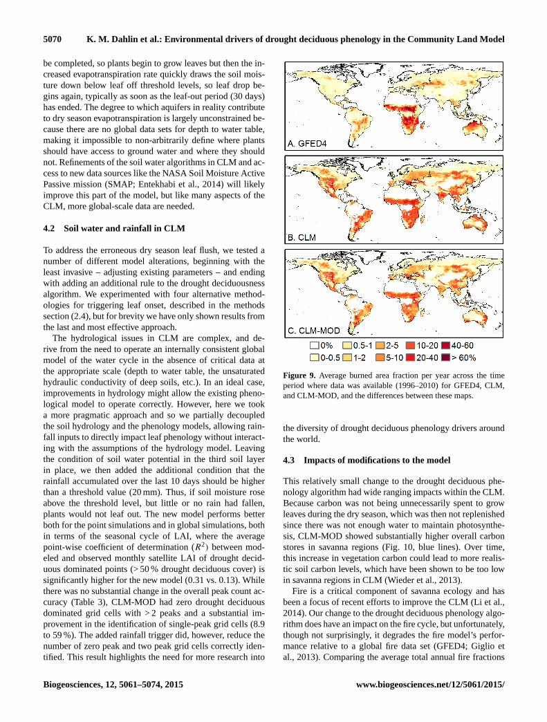
Figure 9. Average burned area fraction per year across the time

period where data was available (1996–2010) for GFED4, CLM,

and CLM-MOD, and the differences between these maps.

the diversity of drought deciduous phenology drivers around

the world.

4.3 Impacts of modifications to the model

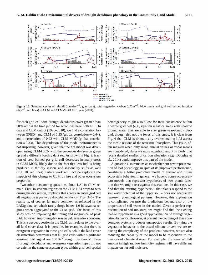
This relatively small change to the drought deciduous phe-

nology algorithm had wide ranging impacts within the CLM.

Because carbon was not being unnecessarily spent to grow

leaves during the dry season, which was then not replenished

since there was not enough water to maintain photosynthe-

sis, CLM-MOD showed substantially higher overall carbon

stores in savanna regions (Fig. 10, blue lines). Over time,

this increase in vegetation carbon could lead to more realis-

tic soil carbon levels, which have been shown to be too low

in savanna regions in CLM (Wieder et al., 2013).

Fire is a critical component of savanna ecology and has

been a focus of recent efforts to improve the CLM (Li et al.,

2014). Our change to the drought deciduous phenology algo-

rithm does have an impact on the fire cycle, but unfortunately,

though not surprisingly, it degrades the fire model’s perfor-

mance relative to a global fire data set (GFED4; Giglio et

al., 2013). Comparing the average total annual fire fractions

Biogeosciences, 12, 5061–5074, 2015 www.biogeosciences.net/12/5061/2015/

K. M. Dahlin et al.: Environmental drivers of drought deciduous phenology in the Community Land Model 5071

Figure 10. Seasonal cycles of rainfall (mm day−1; gray bars), total vegetation carbon (g C m−2; blue lines), and grid cell burned fraction

(day−1; red lines) in CLM and CLM-MOD for 1 year (2001).

for each grid cell with drought deciduous cover greater than

50 % across the time period for which we have both GFED4

data and CLM output (1996–2010), we find a correlation be-

tween GFED4 and CLM of 0.35 (global correlation= 0.44),

and a correlation of 0.23 with CLM-MOD (global correla-

tion= 0.33). This degradation of fire model performance is

not surprising, however, given that the fire model was devel-

oped using CLM4.0CN with the erroneous dry season green

up and a different forcing data set. As shown in Fig. 9, frac-

tion of area burned per grid cell decreases in many areas

in CLM-MOD, likely due to the fact that less fuel is being

produced in the dry season, and seasonality shifts as well

(Fig. 10, red lines). Future work will include exploring the

impacts of this change to CLM on fire and other ecosystem

properties.

Two other outstanding questions about LAI in CLM re-

main. First, in savanna regions in the CLM LAI drops to zero

during the dry season, implying that across an entire grid cell

all vegetation is perfectly drought deciduous (Figs. 3–6). The

reality is, of course, far more complex, as reflected in the

LAI3g data set which rarely drops below 1.0 in savanna re-

gions when aggregated to the CLM grid. The focus of this

study was on improving the timing and magnitude of peak

LAI; however, improving dry season values is also a concern.

This is a deeper question in the CLM, as it relates to the over-

all land cover data. It is possible, for example, that there is

evergreen vegetation in these grid cells, while the land cover

classification determines that all grid cells with a significant

seasonal LAI signal are 100 % “drought deciduous”. Even

if drought deciduous and evergreen vegetation types did not

co-exist in the same ecosystem type, within-grid-cell spatial

heterogeneity might also allow for their coexistence within

a whole grid cell (e.g., riparian areas or areas with shallow

ground water that are able to stay green year-round). Sec-

ond, though also not the focus of this study, it is clear from

Fig. 6 that CLM is dramatically overestimating LAI across

the mesic regions of the terrestrial biosphere. This issue, of-

ten masked when only mean annual values or zonal means

are considered, deserves more attention, and it is likely that

recent detailed studies of carbon allocation (e.g., Doughty et

al., 2014) could improve this part of the model.

A question also remains as to whether our new representa-

tion of leaf phenology, in spite of its improved performance,

constitutes a better predictive model of current and future

ecosystem behavior. In general, we hope to construct ecosys-

tem models that represent hypotheses of how plants func-

tion that we might test against observations. In this case, we

find that the existing hypothesis – that plants respond to the

soil water potential of the upper soil – does not adequately

represent phenological patterns. However, this explanation

is complicated because the predictions depend also on the

properties of soil water in the model. Given a perfect rep-

resentation of soil moisture, we might find that the existing

leaf-on hypothesis is a good approximation of average vege-

tation behavior. However, at present the coupling of these two

complex systems produces unexpected results. By tying the

vegetation behavior to the actual climate drivers we are re-

ducing the complexity of the problem; however, we are also

reducing the capacity of the model to be responsive to the

nuances of climate drivers. For example, the same rainfall

amount in high and low humidity regimes will have different

impacts on net soil moisture.

www.biogeosciences.net/12/5061/2015/ Biogeosciences, 12, 5061–5074, 2015

5072 K. M. Dahlin et al.: Environmental drivers of drought deciduous phenology in the Community Land Model

Ideally, models should represent the mechanisms by which

ecological processes operate in as much fidelity as we un-

derstand. The representation of drought phenology is inter-

esting, however, as we suspect that there are many different

phenological strategies in the tropics that the CLM classifies

with the same algorithm (e.g., Archibald and Scholes, 2007).

This means that in the absence of the representation of these

numerous phenological strategies in the model, we are really

representing the net behavior of ecosystems, rather than the

exact mechanisms pertaining to a single species. The fact that

CLM-MOD improved model performance most significantly

in Africa and less so in Australia and South America by

some metrics (Fig. 7) suggests that evolutionary differences

between plants could play a significant role in determining

phenological patterns between continents. In a higher-fidelity

land surface model, we might ideally allow numerous pheno-

logical algorithms to compete for light and water resources,

and the ecosystem LAI profile would reflect the net behavior

of the successful algorithms. This type of modeling is now

theoretically possible (e.g., Fisher et al., 2010, 2015), and

will be investigated in future versions of the CLM.

5 Conclusions

By comparing satellite-derived estimates of LAI to LAI val-

ues produced by the latest version of the CLM, we revealed

a small but significant issue in the CLM – the tendency for

leaves to flush during the dry season in drought deciduous

PFTs due to unrealistic upwards movement of water through

the soil column. We tested a number of different approaches

to address this issue; however, we found that tying leaf flush-

ing to rainfall directly produced results that better matched

the satellite data. While this change to the drought decidu-

ous phenology algorithm does not reflect our understanding

of how plants respond to their environment in the real world,

without better data on soil water movement at scales rele-

vant to global land surface modeling it is difficult to rely on

the soil water model to drive plant physiology. Changing the

drought deciduous phenology algorithm to remove dry sea-

son leaf flushes improved overall LAI values in savanna sys-

tems as well as changed the amount of carbon stored in these

systems and altered the fire cycle. We also emphasize that

this issue would have been impossible to detect with a stan-

dard “benchmarking” type of metric for measuring seasonal-

ity, and it was difficult to identify until daily model outputs

were reported and analyzed (i.e., Fig. 3). Future work will

include exploring different drought deciduous phenology al-

gorithms for different PFTs and testing the importance of this

change in a coupled Earth system model.

Acknowledgements. The authors thank the members of the Ter-

restrial Sciences Section at NCAR for helpful discussions of this

work, and we thank Dr. Ranga Myneni and his group for providing

the LAI3g data set. K. M. Dahlin was funded by an Advanced

Study Program Postdoctoral Fellowship at NCAR. We would also

like to acknowledge the high-performance computing support

from Yellowstone (ark:/85065/d7wd3xhc) provided by NCAR’s

Computational and Information Systems Laboratory. NCAR is

sponsored by the National Science Foundation.

Edited by: T. Keenan

References

Archibald, S. and Scholes, R. J.: Leaf green-up in a semi-arid

African savanna – separating tree and grass responses to envi-

ronmental cues, J. Veg. Sci., 18, 583–594, 2007.

Bivand, R., Keitt, T., and Rowlingson, B.: rgdal: Bindings for

the geospatial data abstraction library, available at: http://cran.

r-project.org/package=rgdal (last access: January 2015), 2013.

Blyth, E., Clark, D. B., Ellis, R., Huntingford, C., Los, S., Pryor,

M., Best, M., and Sitch, S.: A comprehensive set of benchmark

tests for a land surface model of simultaneous fluxes of water

and carbon at both the global and seasonal scale, Geosci. Model

Dev., 4, 255–269, doi:10.5194/gmd-4-255-2011, 2011.

Bonan, G. B., Levis, S., Sitch, S., Vertenstein, M., and Oleson, K.

W.: A dynamic global vegetation model for use with climate

models?: concepts and description of simulated vegetation dy-

namics, Glob. Change Biol., 9, 1543–1566, doi:10.1046/j.1365-

2486.2003.00681.x, 2003.

Bradley, A. V., Gerard, F. F., Barbier, N., Weedon, G. P., Anderson,

L. O., Huntingford, C., Aragão, L. E. O. C., Zelazowski, P., and

Arai, E.: Relationships between phenology, radiation and pre-

cipitation in the Amazon region, Glob. Change Biol., 17, 2245–

2260, doi:10.1111/j.1365-2486.2011.02405.x, 2011.

Delbart, N., Le Toan, T., Kergoat, L., and Fedotova, V.: Re-

mote sensing of spring phenology in boreal regions: A free

of snow-effect method using NOAA-AVHRR and SPOT-

VGT data (1982–2004), Remote Sens. Environ., 101, 52–62,

doi:10.1016/j.rse.2005.11.012, 2006.

Doughty, C. E., Malhi, Y., Arujo-Murakami, A., Metcalfe, D. B.,

Silva-Espejo, J. E., Arroyo, L., Heredia, J. P., Pardo-Toledo,

E., and Mendizabal, L. M.: Allocation trade-offs dominate the

response of tropical forest growth to seasonal and interannual

drought, J. Ecol., 95, 2192–2201, doi:10.1890/13-1507.1, 2014.

Entekhabi, D., Yueh, S., O’Neill, P. E., Kellogg, K. H., Allen, A.,

Bindlish, R., Brown, M., Chan, S., Colliander, A., and Crow, W.

T.: SMAP Handbook, JPL Publication JPL 400-1567, Jet Propul-

sion Laboratory, Pasadena, California, 182 pp., 2014.

Fisher, R., McDowell, N., Purves, D., Moorcroft, P., Sitch, S., Cox,

P., Huntingford, C., Meir, P., and Ian Woodward, F.: Assessing

uncertainties in a second-generation dynamic vegetation model

caused by ecological scale limitations, New Phytol., 187, 666–

681, doi:10.1111/j.1469-8137.2010.03340.x, 2010.

Fisher, R. A., Muszala, S., Verteinstein, M., Lawrence, P., Xu, C.,

McDowell, N. G., Knox, R. G., Koven, C., Holm, J., Rogers,

B. M., Lawrence, D., and Bonan, G.: Taking off the training

wheels: the properties of a dynamic vegetation model without

climate envelopes, Geosci. Model Dev. Discuss., 8, 3293–3357,

doi:10.5194/gmdd-8-3293-2015, 2015.

Giglio, L., Randerson, J. T., and Van Der Werf, G. R.: Analy-

sis of daily, monthly, and annual burned area using the fourth-

Biogeosciences, 12, 5061–5074, 2015 www.biogeosciences.net/12/5061/2015/

K. M. Dahlin et al.: Environmental drivers of drought deciduous phenology in the Community Land Model 5073

generation global fire emissions database (GFED4), J. Geophys.

Res.-Biogeo., 118, 317–328, doi:10.1002/jgrg.20042, 2013.

Guan, K., Wood, E. F., Medvigy, D., Kimball, J., Pan, M., Cay-

lor, K. K., Sheffield, J., Xu, X., and Jones, M. O.: Terrestrial hy-

drological controls on land surface phenology of African savan-

nas and woodlands, J. Geophys. Res.-Biogeo., 119, 1652–1669,

doi:10.1002/2013JG002572, 2014.

Hijmans, R. J. and van Etten, J.: raster: Geographical data analy-

sis and modeling, available at: http://cran.r-project.org/package=

raster (last access: January 2015), 2013.

Jenerette, G. D., Scott, R. L., and Huete, A. R.: Functional dif-

ferences between summer and winter season rain assessed with

MODIS-derived phenology in a semi-arid region, J. Veg. Sci.,

21, 16–30, doi:10.1111/j.1654-1103.2009.01118.x, 2010.

Kelley, D. I., Prentice, I. C., Harrison, S. P., Wang, H., Simard, M.,

Fisher, J. B., and Willis, K. O.: A comprehensive benchmarking

system for evaluating global vegetation models, Biogeosciences,

10, 3313–3340, doi:10.5194/bg-10-3313-2013, 2013.

Koven, C. D., Riley, W. J., Subin, Z. M., Tang, J. Y., Torn, M. S.,

Collins, W. D., Bonan, G. B., Lawrence, D. M., and Swenson,

S. C.: The effect of vertically resolved soil biogeochemistry and

alternate soil C and N models on C dynamics of CLM4, Biogeo-

sciences, 10, 7109–7131, doi:10.5194/bg-10-7109-2013, 2013.

Lau, W. K.-M., Wu, H.-T., and Kim, K.-M.: A canonical

response of precipitation characteristics to global warming

from CMIP5 models, Geophys. Res. Lett., 40, 3163–3169,

doi:10.1002/grl.50420, 2013.

Lawrence, D. M., Oleson, K. W., Flanner, M. G., Thornton, P. E.,

Swenson, S. C., Lawrence, P. J., Zeng, X., Yang, Z.-L., Levis, S.,

Sakaguchi, K., Bonan, G. B., and Slater, A. G.: Parameterization

improvements and functional and structural advances in Version

4 of the Community Land Model, J. Adv. Model. Earth Syst., 3,

M03001, doi:10.1029/2011MS000045, 2011.

Lawrence, D. M., Oleson, K. W., Flanner, M. G., Fletcher, C. G.,

Lawrence, P. J., Levis, S., Swenson, S. C., and Bonan, G. B.:

The CCSM4 Land Simulation, 1850–2005: Assessment of Sur-

face Climate and New Capabilities, J. Climate, 25, 2240–2260,

doi:10.1175/JCLI-D-11-00103.1, 2012.

Lawrence, P. J. and Chase, T. N.: Representing a new MODIS con-

sistent land surface in the Community Land Model (CLM 3.0), J.

Geophys. Res., 112, G01023, doi:10.1029/2006JG000168, 2007.

Li, F., Bond-Lamberty, B., and Levis, S.: Quantifying the role of fire

in the Earth system – Part 2: Impact on the net carbon balance

of global terrestrial ecosystems for the 20th century, Biogeo-

sciences, 11, 1345–1360, doi:10.5194/bg-11-1345-2014, 2014.

Ma, X., Huete, A., Yu, Q., Coupe, N. R., Davies, K., Broich, M.,

Ratana, P., Beringer, J., Hutley, L. B., Cleverly, J., Boulain,

N., and Eamus, D.: Spatial patterns and temporal dynam-

ics in savanna vegetation phenology across the North Aus-

tralian Tropical Transect, Remote Sens. Environ., 139, 97–115,

doi:10.1016/j.rse.2013.07.030, 2013.

McKay, M. D., Beckman, R. J., and Conover, W. J.: Comparison

of Three Methods for Selecting Values of Input Variables in the

Analysis of Output from a Computer Code, Technometrics, 21,

239–245, doi:10.1080/00401706.1979.10489755, 1979.

Oleson, K. W., Lawrence, D. M., Bonan, G. B., Drewniak, B.,

Huang, M., Koven, C., Levis, S., Li, F., Riley, W., Subin, Z.,

Swenson, S., Thornton, P. E., Bozbiyik, A., Fisher, R., Heald, C.,

Kluzek, E., Lamarque, J.-F., Lawrence, P., Leung, L., Lipscomb,

W., Muszala, S., Ricciuto, D., Sacks, W., Sun, Y., Tang, J., and

Yang, Z. L.: Technical description of version 4.5 of the Commu-

nity Land Model (CLM), NCAR Tech. Note, 503+STR(June),

doi:10.5065/D6RR1W7M, 2013.

Parmesan, C. and Yohe, G.: A globally coherent fingerprint of cli-

mate change impacts across natural systems, Nature, 421, 37–42,

doi:10.1038/nature01286, 2003.

Pierce, D.: ncdf: Interface to unidata netCDF files, available at: http:

//cran.r-project.org/package=ncdf (last access: January 2015),

2011.

Randerson, J. T., Hoffman, F. M., Thornton, P. E., Mahowald, N.

M., Lindsay, K., Lee, Y.-H., Nevison, C. D., Doney, S. C., Bo-

nan, G., Stöckli, R., Covey, C., Running, S. W., and Fung, I.

Y.: Systematic assessment of terrestrial biogeochemistry in cou-

pled climate-carbon models, Glob. Change Biol., 15, 2462–2484,

doi:10.1111/j.1365-2486.2009.01912.x, 2009.

R Core Team: R Development Core Team: Environ. Stat. Com-

put., available at: http://www.R-project.org (last access: January

2015), 2013.

Reed, B. C., Schwartz, M. D., and Xiao, X.: Remote sensing phe-

nology: Status and the way forward, in: Phenology of Ecoystem

Processes: Applications in global change research, edited by: A.

Noormets, 231–246, Springer Science + Business Media LLC,

Dordrecht, Heidelberg, London, New York, 2009.

Reich, P. B.: Phenology of tropical forests: Patterns, causes, and

consequences, Can. J. Bot., 73, 164–174, 1995.

Richardson, A. D., Anderson, R. S., Arain, M. A., Barr, A. G.,

Bohrer, G., Chen, G., Chen, J. M., Ciais, P., Davis, K. J., De-

sai, A. R., Dietze, M. C., Dragoni, D., Garrity, S. R., Gough,

C. M., Grant, R., Hollinger, D. Y., Margolis, H. a., McCaughey,

H., Migliavacca, M., Monson, R. K., Munger, J. W., Poulter, B.,

Raczka, B. M., Ricciuto, D. M., Sahoo, A. K., Schaefer, K., Tian,

H., Vargas, R., Verbeeck, H., Xiao, J., and Xue, Y.: Terrestrial

biosphere models need better representation of vegetation phe-

nology: results from the North American Carbon Program Site

Synthesis, Glob. Change Biol., 18, 566–584, doi:10.1111/j.1365-

2486.2011.02562.x, 2012.

Scholes, R. J. and Hall, D. O.: The carbon budget of tropical sa-

vannas, woodlands, and grassslands, in SCOPE 56 – Global

Change: Effects on Coniferous forests and grasslands, edited by:

Breymeyer, A. I., Hall, D. O., Melillo, J. M., and Agren, G. I.,

John Wiley & Sons Ltd, Chichester, UK, 1996.

Staver, A. C., Archibald, S., and Levin, S. A.: The global extent and

determinants of savanna and forest as alternative biome states,

Science, 334, 230–232, doi:10.1126/science.1210465, 2011.

Swenson, S. C. and Lawrence, D. M.: Assessing a dry surface layer-

based soil resistance parameterization for the Community Land

Model using GRACE and FLUXNET-MTE data, J. Geophys.

Res.-Atmos., 119, 299–312, doi:10.1002/2014JD022314, 2014.

Viovy, N.: CRU-NCEP Version 4, available at: http://dods.extra.

cea.fr/data/p529viov/cruncep/V4_1901_2012/ last access: Au-

gust 2012.

Wang, K., Mao, J., Dickinson, R., Shi, X., Post, W., Zhu, Z., and

Myneni, R.: Evaluation of CLM4 Solar Radiation Partitioning

Scheme Using Remote Sensing and Site Level FPAR Datasets,

Remote Sens., 5, 2857–2882, doi:10.3390/rs5062857, 2013.

White, M. A., Thornton, P. E., and Running, S. W.: A continental

phenology model for monitoring vegetation responses to interan-

www.biogeosciences.net/12/5061/2015/ Biogeosciences, 12, 5061–5074, 2015

5074 K. M. Dahlin et al.: Environmental drivers of drought deciduous phenology in the Community Land Model

nual climatic variability, Global Biogeochem. Cy., 11, 217–234,

doi:10.1029/97GB00330, 1997.

White, M. A., de BEURS, K. M., Didan, K., Inouye, D. W.,

Richardson, A. D., Jensen, O. P., O’Keefe, J., Zhang, G., Ne-

mani, R. R., van LEEUWEN, W. J. D., Brown, J. F., de WIT,

A., Schaepman, M., Lin, X., Dettinger, M., Bailey, A. S., Kim-

ball, J., Schwartz, M. D., Baldocchi, D. D., Lee, J. T., and

Lauenroth, W. K.: Intercomparison, interpretation, and assess-

ment of spring phenology in North America estimated from re-

mote sensing for 1982–2006, Glob. Change Biol., 15, 2335–

2359, doi:10.1111/j.1365-2486.2009.01910.x, 2009.

Wieder, W. R., Bonan, G. B., and Allison, S. D.: Global soil car-

bon projections are improved by modelling microbial processes,

Nature Climate Change, 3, 909–912, doi:10.1038/nclimate1951,

2013.

Yang, X., Mustard, J. F., Tang, J., and Xu, H.: Regional-scale

phenology modeling based on meteorological records and re-

mote sensing observations, J. Geophys. Res., 117, G03029,

doi:10.1029/2012JG001977, 2012.

Zhang, X., Friedl, M. A., Schaaf, C. B., and Strahler, A. H.: Mon-

itoring the response of vegetation phenology to precipitation in

Africa by coupling MODIS and TRMM instruments, J. Geophys.

Res., 110, D12103, doi:10.1029/2004JD005263, 2005.

Zhu, Z., Bi, J., Pan, Y., Ganguly, S., Anav, A., Xu, L., Samanta,

A., Piao, S., Nemani, R., and Myneni, R.: Global Data Sets of

Vegetation Leaf Area Index (LAI)3g and Fraction of Photosyn-

thetically Active Radiation (FPAR)3g Derived from Global In-

ventory Modeling and Mapping Studies (GIMMS) Normalized

Difference Vegetation Index (NDVI3g) for the Period 1981 to 2,

Remote Sens., 5, 927–948, doi:10.3390/rs5020927, 2013.

Biogeosciences, 12, 5061–5074, 2015 www.biogeosciences.net/12/5061/2015/