environmental costs and benefits - piie · 2014. 1. 3. · shale gas drilling sites (mckenzie et...

99

7Environmental Costs and Benefits

For all the recent excitement about the potential economic and national secu-rity benefits of the US oil and gas boom, there is equal, if not greater, concern about its potential environmental consequences. The Deepwater Horizon oil spill in the Gulf of Mexico in 2010 dominated national media for weeks on end, the Keystone XL oil pipeline became a prominent issue in the 2012 presiden-tial election, and protests against hydrofracking have become a regular part of life in many energy-rich states. In the previous chapters we have attempted to quantify the economic effects of the oil and gas boom. It is equally important to quantify its environmental costs and benefits. A proper analysis is beyond the scope of this book, but this chapter offers a brief discussion of the envi-ronmental implications of unconventional oil and gas development and how policy can mitigate its negative effects.

Water, Air, and Earthquakes

Most of the environmental concern surrounding increased oil and gas develop-ment has focused on local effects in the communities where the development is occurring, regarding water resources in particular. In addition to taking the lives of eleven people, the Deepwater Horizon explosion significantly damaged Gulf Coast ecosystems, including beaches, wetlands, and commercial fisheries. And a couple of high-profile pipeline accidents in recent years have raised concerns about onshore water contamination risks from oil and gas develop-ment.1 But the potential effect of hydraulic fracturing, or fracking, on local water supplies has received the most attention.

1. See, e.g., EPA, “EPA’s Response to the Enbridge Oil Spill,” www.epa.gov/enbridgespill (accessed on September 8, 2013).

© Peterson Institute for International Economics | www.piie.com

100 Fueling up

As discussed in chapter 2, fracking is performed by injecting pressurized water, sand, and additives into a wellbore to create fissures in semipermeable shale or tight gas reservoirs. This releases trapped natural gas, which, along with the fluid used to fracture the well, flows back up the wellbore. While shale and gas reservoirs are generally located between 3,000 and 12,000 feet below the surface, wells often pass through groundwater reservoirs before reaching shale (EIA 2011c). The wellbore is sealed in cement to protect groundwater supplies, but many environmental and community groups are concerned that the chemicals used in fracking could still find their way into local water supplies. Similar concerns surround wastewater disposal.

In 2008 the residents of Pavillion, Wyoming, began complaining about discolored and foul-smelling local water, prompting an Environmental Protection Agency (EPA) investigation. In 2011 the EPA issued a draft report concluding that contaminants found in the town’s water likely came from nearby natural gas drilling (EPA 2011a).2 Of the tens of thousands of gas wells that have been fracked in recent years, this was the first government finding of groundwater contamination, and it was from a tight gas rather than a shale gas well. Still, it has heightened public concern about the environmental costs of the oil and gas boom. Rather than fracking chemicals, methane—what natural gas is made of—has been found in the water supply in a number of areas where gas development is occurring (Osborn et al. 2011). This could be from the drilling process, or it could have naturally migrated into the water reservoir from the shale formation. Methane is not toxic, but it can be highly flammable—a characteristic most people generally do not look for in drinking water. The EPA is conducting a comprehensive study of the effects of fracking on drinking water and groundwater, to be completed in 2014. This assessment will likely serve as the scientific basis for any water-related federal regulation of fracking in the years ahead.

Water contamination is not the only concern surrounding the under-ground injection of fracking fluids or wastewater management. While the overwhelming majority of earthquakes have natural causes, some are attrib-utable to human activity. These so-called induced seismic events have been documented since the 1920s and can be traced to activities ranging from coal mining to geothermal energy development. The vast majority of documented energy-related induced seismic events occurred due to geothermal develop-ment (NRC et al. 2012). But oil and gas extraction can induce seismic events as well if injection or withdrawal of fluids significantly alters subsurface pressure balances. Such occurrences are rare, and have been largely caused by enhanced oil recovery techniques, such as water flooding. Only one induced seismic event

2. The industry disputes many EPA draft report findings. See, e.g., Christopher Helman, “Questions Emerge on EPA’s Wyoming Fracking Study,” Forbes, December 9, 2011, www.forbes.com/sites/christopherhelman/2011/12/09/questions-emerge-on-epas-wyoming-fracking-study (accessed on September 8, 2013).


environmental Costs and BeneFits 101

(2.8 magnitude) in the United States is suspected to have been caused by the injection of fracking fluids into a shale gas well, and one event in the United Kingdom has been conclusively linked to shale gas development. Of greater concern is the injection of wastewater, either from conventional or shale devel-opment, into disposal wells.

Finally, oil and gas development can create air quality problems in the communities where drilling is occurring. Diesel-powered trucks and drilling equipment emit particulate matter and sulfur dioxide, and oil and gas drilling—hydrofracking in particular—is a leading source of volatile organic compound emissions, which contribute to the formation of ground-level ozone.3 Ozone exposure contributes to aggravated asthma and other respiratory illnesses. Oil and gas development also emits air toxics, such as benzene, ethylbenzene, and n-hexane, and studies have found high concentrations of airborne toxins near shale gas drilling sites (McKenzie et al. 2012). As unconventional gas devel-opment has accelerated, air quality complaints in communities in Wyoming, Texas, Pennsylvania, and other gas-rich states have become more prominent.4

Environmental Upside

The oil and gas boom is delivering environmental benefits as well as costs. While natural gas prices have plummeted in recent years, thanks to growth in shale and other unconventional supply, the price US power plants pay for coal has risen. Between 2000 and 2007, power plants paid $1.42 per million British thermal units (MMBtu), on average, for coal, compared with $5.81 for natural gas (EIA 2013d). During 2010 and 2011, delivered coal prices rose to an average of $2.30 per MMBtu while gas prices fell to $4.90, and in 2012, delivered coal and natural gas prices were $2.41 and $3.43 respectively, the smallest spread since the early 1970s (EIA 2013d).

As the gap between coal and natural gas prices narrowed, natural gas-fired power plants were able to outcompete coal-fired power plants in competitive wholesale markets in many parts of the country. A number of power companies started switching their generation portfolio away from coal to natural gas. As a result, coal’s share of US power generation fell from 48 percent during 2008 to a record low of 32.6 percent in April 2012. Natural gas’ share rose from 21 percent to 32.2 percent over the same period, coming close to overtaking coal as the leading source of power generation in the United States (EIA 2013d).

Burning natural gas emits fewer air pollutants, such as sulfur dioxide (SO2), nitrogen oxide (NOx), and mercury, than burning coal. Natural gas-fired power plants are also, on average, more efficient than their coal-fired peers, meaning

3. For more information, see EPA, “Oil and Natural Gas Air Pollution Standards,” http://epa.gov/airquality/oilandgas/basic.html (accessed on September 8, 2013).

4. Kirk Johnson, “In Pinedale, Wyo., Residents Adjust to Air Pollution,” New York Times, March 9, 2011.


102 Fueling up

that they need less fuel to generate the same amount of electricity. So with the power sector switching from coal to natural gas, US air pollution levels have fallen. The EPA estimates that between 2008 and 2012, US sulfur dioxide emis-sions fell by 15 percent per year, three times the average annual rate between 2000 and 2008 (EPA 2012c). The power sector accounted for 94 percent of this decline. It is difficult to assess exactly how much of this drop was due to coal-to-natural gas fuel switching, as power plants have other options for reducing SO2 emissions, such as installing pollution control technology or switching to lower-sulfur coals. Slower power demand growth between 2008 and 2012 also played an important role. But the economic benefit of the overall reduction in power sector SO2 emissions is significant. The National Research Council (NRC 2009) estimates that each ton of SO2 emitted from a coal-fired power plant costs the United States $5,800 in environmental and human health damages. At these numbers, the decline in power sector SO2 emissions between 2008 and 2012 saves the country $26 billion per year.

Switching from coal to natural gas in the power sector has had a smaller but also important effect on NOx emissions (EPA 2012c). Between 2008 and 2012, NOx emissions declined twice as fast as between 2000 and 2008, with the power sector accounting for 23 percent of the drop (the transportation sector is responsible for the rest). The NRC also estimates that each ton of NOx emitted costs the country $1,600. At that rate, the decline in power sector NOx emissions between 2008 and 2012 saves the country an additional $2 billion per year. Switching from coal to natural gas also lowers mercury and particu-late matter pollution, but recent emissions data are not available.

Climate Breakthrough?

Beyond local air pollution reductions, the oil and gas boom has delivered some global environmental benefits as well. At the UN climate change summit in Copenhagen in 2009, the United States pledged to reduce greenhouse gas emissions 17 percent below 2005 levels by 2020 (Houser 2010). This pledge was conditioned on enactment of domestic cap-and-trade legislation that had passed the House of Representatives that spring (UNFCCC 2009). After the Copenhagen summit concluded, however, cap-and-trade legislation died in the Senate and never made it to President Obama’s desk to sign. In the face of this legislative failure and the Republican takeover of the House of Representatives in 2010, environmental activists worried the United States would not be able to achieve its target and that other countries would moderate their emission reduction efforts in response.

Yet despite the absence of federal policy, US emissions have fallen sharply in recent years, raising hopes that the United States might still be able to reach its 2020 goal. In 2012, energy-related CO2 emissions, which account for 79 percent of total US greenhouse gas (GHG) emissions, were 12 percent below 2005 levels (figure 7.1). That is a sharper decline than in the European Union, which has an economywide climate policy; there, CO2 emissions in 2012 were

1

2000 2001 2002 2003 2004 2005 2006 2007 2008 2009 2010 2011 2012

United States EU-274.1

4.0

3.9

3.8

3.7

3.6

3.5

3.4

3.3

3.2

6.0

5.8

5.6

5.4

5.2

5.0

4.8

Figure 7.1 Energy-related CO2 emissions, United States versus EU-27, 2000–12 (billions of tons)

EU-27 (right axis)

United States (left axis)

Note: 2012 �gures are annualized estimates from �rst half data.

Sources: United Nations Framework Convention on Climate Change; EuroStat; Energy Information Administration.

zz--Figs_Ch7.indd 1 11/7/13 12:10 PM



down 10 percent from 2005 levels (figure 7.1).5 It is also a dramatic departure from what most analysts, until recently, expected to occur. In 2006 the Energy Information Administration (EIA) forecast that energy-related CO2 emissions in the United States would increase by 9 percent between 2005 and 2012 to 6,536 million tons (figure 7.2). Actual emissions in 2012 were 5,290 million tons, their lowest level since 1994.

What explains the unexpected drop? In the broadest terms, the amount of CO2 a country emits is determined by the level of economic activity (measured in GDP), the amount of energy consumed per unit of GDP (energy intensity), and the amount of CO2 emitted per unit of energy consumed (carbon inten-sity). A significant change in any one of these factors can alter a country’s CO2

5. The Europeans prefer to measure reductions against a 1990 baseline, the base year for Kyoto Protocol commitments. Against 1990 levels, US emissions were up by 7 percent in 2012, com-pared with a 13 percent decline for the European Union. Also, the EU Emissions Trading Scheme allows companies and countries to meet their compliance obligations by purchasing emissions reductions, called offsets, from other parts of the world instead of reducing emissions at home. Including offsets in the above calculation increases overall EU emissions reductions relative to the United States.

1

2000 2001 2002 2003 2004 2005 2006 2007 2008 2009 2010 2011 2012

United States EU-274.1

4.0

3.9

3.8

3.7

3.6

3.5

3.4

3.3

3.2

6.0

5.8

5.6

5.4

5.2

5.0

4.8

Figure 7.1 Energy-related CO2 emissions, United States versus EU-27, 2000–12 (billions of tons)

EU-27 (right axis)

United States (left axis)

Note: 2012 �gures are annualized estimates from �rst half data.

Sources: United Nations Framework Convention on Climate Change; EuroStat; Energy Information Administration.

zz--Figs_Ch7.indd 1 11/7/13 12:10 PM


104 Fu

eling

up

2

AEO 2006

Actual

7,000

6,500

6,000

5,500

5,000

4,500

4,000

1985198619871988198919901991199219931994199519961997199819992000200120022003200420052006200720082009201020112012

millions of tons

Figure 7.2 Actual energy-related US CO2 emissions versus EIA 2006 projections, 1985–2012

EIA = Energy Information Administration; AEO = Annual Energy Outlook

Sources: EIA (2006, 2012b, 2013d).

zz--Figs_C

h7.indd 210/18/13 1:10 P

M

3

Projectedem

issionsActual

emissions

Economic

growth

Energy intensity

of the econom

yCarbon

intensityof energy

–819

–74

–353

5,290

6,536

7,000

6,500

6,000

5,500

5,000

4,500

4,000

3,500

millions of tons

Figure 7.3 D

i�erence betw

een actual CO2 em

issions in 2012 and EIA

2006 projections, by source of change

Sources: EIA (2006, 2013d).

zz--Figs_C

h7.indd 311/7/13 12:10 P

M



emissions trajectory. The EIA projected in 2006 that the US economy would grow by 3.1 percent a year between 2005 and 2012, continuing its average rate of GDP growth between 1990 and 2005. The energy intensity of the economy was expected to decline by 1.65 percent a year, down a bit from the 1990–2005 annual average of 1.86 percent due primarily to a slowdown in the US econo-my’s transition from manufacturing (more energy intensity) to service sector (less energy intensive) activity. The carbon intensity of energy supply was projected to remain the same, with the shares coming from coal, natural gas, oil, nuclear, and renewables holding relatively constant.

However, due to the financial crisis, the economy expanded much less than projected, with GDP growth averaging 1.1 percent between 2005 and 2012. That alone accounts for 66 percent of the difference between projected and actual emissions in 2012, or 819 million tons (figure 7.3).6 Energy intensity

6. For this attribution, we adopt a similar methodology to the Council of Economic Advisers (CEA 2013) in their 2013 Economic Report of the President. CO2 emissions are the product of (CO2/BTU) × (BTU/GDP) × GDP, where CO2 represents US CO2 emissions in a given year, BTU represents energy consumption in that year, and GDP is that year’s GDP. We take logarithms of this expres-sion and subtract the baseline from the actual values to attribute reductions to slower economic growth, less energy-intensive economic activity, and lower carbon intensity of energy supply. The

3

Projectedemissions

Actualemissions

Economicgrowth Energy

intensityof the

economyCarbon

intensityof energy

–819

–74

–353

5,290

6,536

7,000

6,500

6,000

5,500

5,000

4,500

4,000

3,500

millions of tons

Figure 7.3 Di�erence between actual CO2 emissions in 2012 and EIA 2006 projections, by source of change

Sources: EIA (2006, 2013d).

zz--Figs_Ch7.indd 3 11/7/13 12:10 PM


106 Fueling up

declined faster than expected (1.80 percent per year instead of 1.65 percent) because of high energy prices and improved efficiency in vehicles, buildings, and industry. That accounts for 6 percent of the decline, or 74 million tons. The carbon intensity of energy supply fell to all-time lows, delivering the remaining 28 percent of the downside surprise in US emissions, or 353 million tons. Thus a number of developments between 2005 and 2012 contributed to the decline in the carbon intensity of US energy supply. As discussed in chapter 5, increased ethanol production allowed for fuel switching in the transpor-tation sector. Ethanol and other biofuels emit CO2 when they are produced and when they are combusted, but the plants used as feedstock also sequester CO2 as they grow. Based on EIA data, fuel switching in the transportation sector accounted for nearly 15 percent of the reduction in the carbon intensity of overall US energy supply between 2005 and 2012.7 Fuel switching in the industrial sector accounted for 7 percent of the economywide carbon inten-sity reductions, thanks primarily to biomass substituting for coal in industrial boilers.

The greatest shift, however, occurred in the electric power sector (figure 7.4), as the market share of coal—the most carbon-intensive fuel used in power generation—declined from 51 percent to 38.5 percent.8 Oil, the power sector’s second most carbon-intensive fuel source, saw its share of generation fall from 3 percent to 0.5 percent. Meanwhile, zero-carbon sources of power generation, such as nuclear and renewables, grew from 28.2 percent to 31.5 percent, thanks primarily to an increase in wind generation. Natural gas saw even bigger gains,

CEA findings are slightly different from ours for two reasons. First, the CEA uses projected 2012 emissions, as full-year data were not yet available at the time of publication. Second and more im-portant, they use a lower GDP growth estimate in their business-as-usual projection than the 3.1 percent used in the EIA 2006 projections. This reflects recent academic and government estimates that potential GDP growth in the United States has slowed to 2.5 to 2.6 percent. This is the right approach for attributing how much of the decline in emissions was due to the recession, whereas our approach compares actual GDP growth with projected GDP growth, with the difference cov-ering both the recession and slower potential GDP growth than forecast in 2006.

7. The EIA energy-related CO2 emissions data on which figures 7.1 to 7.4 are based capture the emissions released in the conversion of corn, sugar, oil, or other feedstock to biofuels, provided it occurs domestically, but in the industrial, not transportation, sector data. This is similar to petro-leum products, where the emissions from gasoline combustion are included in the transportation sector data but emissions from crude oil refining are included in the industrial sector. A proper accounting of the net emissions effect of switching from petroleum to biofuels should include the emissions involved in producing both fuels, as well as combusting them, and would likely change the sectoral distribution of carbon-intensity reductions shown in figure 7.4. More important, EIA energy-related CO2 data exclude emissions from biofuels combustion, assuming that the produc-tion of biofuel feedstocks sequesters an equal quantity of CO2. While narrowly correct, increased biofuel production can lead to broader land-use change that could lead to a net decline in forest sequestration, offsetting some of the emissions benefit of switching from petroleum to ethanol or biodiesel. The EIA does not include land-use change estimates in either the overall or transport sector CO2 data.

8. Generation in the electric power sector only. Data taken from EIA (2013d, table 7.2b).



growing from 17.5 percent of generation in 2005 to 29.2 percent in 2012 (EIA 2012d).

Switching from coal to natural gas for power generation has less of an effect on CO2 emissions than on SO2, NOx and mercury pollution. While less carbon intensive than coal or oil, natural gas combustion still emits meaningful quan-tities of CO2 while emitting very little NOx and almost no SO2 or mercury. On average, coal-fired power generation in the United States emits 2,249 pounds per megawatt hours (lbs/MWh) of carbon dioxide, 13 lbs/MWh of sulfur di-oxide, and 6 lbs/MWh of nitrogen oxides. Natural gas-fired power generation emits 1,135 lbs/MWh of CO2, 0.1 lbs/MWh of SO2, and 1.7 lbs/MWh of NOx.

9

Determining exactly how much of the decline in the carbon intensity of US power generation is attributable to natural gas is challenging. For a rough esti-mate, we proportionally allocated the decline in coal’s and oil’s market shares in the electric power sector, and associated CO2 emissions, between 2005 and 2012 to natural gas, nuclear, and renewables, based on the growth in each fuel’s market share over the same period, factoring in CO2 emissions from natural gas generation. Based on this approach, expanded use of natural gas accounted for 65 percent of the decarbonization of the power sector between 2005 and 2012, followed by wind at 30 percent, with nonwind renewables accounting for the rest. This approach, however, assumes that a kilowatt hour (kWh) displaced

9. EPA, “Air Emissions,” www.epa.gov/cleanenergy/energy-and-you/affect/air-emissions.html (ac-cessed on September 8, 2013).

4

4.11.4

7.3

14.7

Residential Commercial Industrial Transportation Power generation

80

70

60

50

40

30

20

10

0

72.5

percent

Figure 7.4 Reduction in the carbon intensity of primary energy consumption, by sector, 2012 versus 2005

Source: EIA (2013d).

zz--Figs_Ch7.indd 4 10/18/13 1:10 PM


108 Fueling up

by additional natural gas generation has the same carbon intensity as a kWh displaced by renewable generation. In reality, there are important regional differences in the competition between and dispatch profiles of different fuels, which a more robust attribution analysis would account for.10 But it is safe to say that while the recession accounted for most of the decline in US emissions between 2005 and 2012, decarbonization of the power sector played an impor-tant role, and that was primarily due to low-cost natural gas.

Limits of Cheap Natural Gas

Emission reductions driven by cheap gas alone, however, appear to have run their course. While coal-fired power hit a record low of 33 percent of total US generation in April 2012 thanks to a shale-driven decline in natural gas costs, prices recovered during the second half of the year. By the end of 2012, the price of natural gas delivered to US power plants was up 57 percent and coal’s market share had climbed back to 40 percent (EIA 2013d). A relatively cold winter continued to put upward pressure on natural gas prices into 2013, keeping coal competitive in the power sector. And overall electricity demand is growing slightly due to continued, though painfully slow, economic recovery. In its most recent short-term energy outlook as of the time of writing, the EIA predicted that US CO2 emissions will rise by 3 percent in 2013.

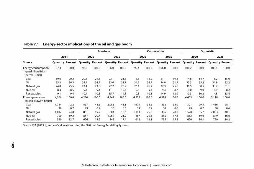
Over the longer term, our modeling suggests that should more optimistic production forecasts pan out, the oil and gas boom will help keep power sector emissions growth in check but have only a modest net effect on US emissions overall. In our pre-shale scenario, coal maintains a 42 to 43 percent share of US power generation throughout the projection period (table 7.1 and figure 7.5). Overall power demand grows by just under 20 percent between 2013 and 2035, and coal-fired power generation moves with it. In our conservative scenario, coal’s market share declines to 38 percent by 2016 and holds steady in percentage terms through 2035, resulting in modest absolute growth. In our optimistic case, however, coal-fired power generation falls from 1,734 billion kWh in 2011 to 1,285 billion kWh in 2016, then grows at half the rate of power generation overall. As a result, coal’s share falls to 30 percent by 2020 and 28 percent by 2035.

Natural gas picks up the slack, with generation doubling between 2011 and 2035. By 2035 natural gas accounts for 40 percent of all power generation in our optimistic scenario, compared with 17 percent in the pre-shale case. Some of this growth comes at the expense of nuclear and renewables as well as coal. Nuclear generation grows by 7 percent between 2011 and 2035 in our

10. For a discussion of this point, see Trevor Houser, “More on the Recent US Emissions Decline,” Rhodium Group, March 4, 2013, http://rhg.com/notes/more-on-the-recent-us-emissions-decline (accessed on September 8, 2013) and Michael Shellenberger, Ted Nordhaus, Alex Trembath, and Max Luke, “Debunking Rhodium,” Breakthrough Institute, http://thebreakthrough.org/index.php/debunking-rhodium/ (accessed on September 8, 2013).


envir

on

men

tal C

osts a

nd

Ben

eFits 109

15

Table 7.1 Energy-sector implications of the oil and gas boom

Pre-shale Conservative Optimistic

2011 2020 2035 2020 2035 2020 2035

Source Quantity Percent Quantity Percent Quantity Percent Quantity Percent Quantity Percent Quantity Percent Quantity Percent

Energy consumption (quadrillion British thermal units)

97.3 100.0 98.5 100.0 106.0 100.0 99.4 100.0 106.8 100.0 100.2 100.0 108.4 100.0

Coal 19.6 20.2 20.8 21.1 23.1 21.8 18.8 18.9 21.1 19.8 14.8 14.7 16.2 15.0Oil 35.3 36.3 34.4 34.9 33.6 31.7 34.7 34.9 34.0 31.9 35.3 35.2 34.9 32.2Natural gas 24.8 25.5 23.4 23.8 22.2 20.9 26.1 26.2 27.3 25.6 30.5 30.5 33.7 31.1Nuclear 8.3 8.5 9.3 9.4 11.1 10.5 9.3 9.3 9.3 8.7 9.0 9.0 8.9 8.2Renewables 9.1 9.4 10.4 10.5 15.7 14.8 10.3 10.3 14.9 13.9 10.3 10.3 14.5 13.4

Power generation (billion kilowatt hours)

4,106 100.0 4,280 100.0 4,844 100.0 4,333 100.0 4,979 100.0 4,403 100.0 5,118 100.0

Coal 1,734 42.2 1,867 43.6 2,086 43.1 1,674 38.6 1,892 38.0 1,301 29.5 1,436 28.1Oil 28 0.7 29 0.7 30 0.6 29 0.7 30 0.6 29 0.7 30 0.6Natural gas 1,017 24.8 851 19.9 804 16.6 1,111 25.6 1,396 28.0 1,570 35.7 2,053 40.1Nuclear 790 19.2 887 20.7 1,062 21.9 887 20.5 885 17.8 862 19.6 849 16.6Renewables 520 12.7 626 14.6 842 17.4 612 14.1 755 15.2 620 14.1 729 14.2

Source: EIA (2013d); authors’ calculations using the National Energy Modeling System.


110 Fueling up 5

Coal Natural gasPetroleum NuclearHydro Other renewables

Figure 7.5 Power generation by source under current policy, 2011–35

Source: Authors’ calculations using the National Energy Modeling System.

4,500

4,000

3,500

3,000

2,500

2,000

1,500

1,000

500

0

5,500

5,000

20112012

20132014

20152016

20172018

20192020

20212022

20232024

20252026

20272028

20292030

20312032

20332034

2035

a. Pre-shale

billion kilowatt hours (percent share in shaded areas)

58

19

25

42

11

7

22

17

43

4,500

4,000

3,500

3,000

2,500

2,000

1,500

1,000

500

0

5,500

5,000

20112012

20132014

20152016

20172018

20192020

20212022

20232024

20252026

20272028

20292030

20312032

20332034

2035

b. Optimistic


58

19

25

42

8

6

17

40

28

zz--Figs_Ch7.indd 5 11/7/13 12:10 PM



optimistic scenario, compared with 34 percent in the pre-shale case. Renewable generation still experiences a healthy 40 percent expansion between 2011 and 2035, but that is down from 62 percent in the pre-shale scenario (table 7.1). That means that by 2035 renewables account for 9 percent of total power generation instead of 11 percent.

That natural gas displaces some nuclear and renewables is not so bad from a local air pollution standpoint, as long as it is also displacing coal. Between 2013 and 2035 annual SO2 emissions from the electric power sector are 10.6 percent and 35.4 percent lower on average in our conservative and optimistic scenarios compared with the pre-shale case (figure 7.6). NOx emissions are 2.4 percent and 16.4 percent lower, while mercury emissions are 7.6 and 25.3 percent lower. In the pre-shale scenario SO2, NOx, and mercury emissions are already projected to decline, thanks to already adopted EPA regulations. Still, the difference in power sector SO2 and NOx emissions between the optimistic and pre-shale scenarios would deliver nearly $6 billion a year in additional economic savings using the NRC’s damage estimates, and likely several billion more in annual savings from lower mercury emissions.

For CO2, however, the long-term effect of the oil and gas boom is more modest. In our projections, there is little difference in US CO2 emissions between the pre-shale and conservative scenarios, and in the optimistic scenario CO2 emissions are only 109 million tons lower on average between 2013 and 2035 than in the pre-shale case (figure 7.7). Natural gas generation displaces some nuclear and renewables, as well as coal, which blunts its climate benefit

6

40

35

30

25

20

15

10

5

0SO

2NO

xMercury

10.6

2.4

16.4

7.6

25.3

35.4

Optimistic

Conservative

Source: Authors’ calculation using the National Energy Modeling System.

percent

Figure 7.6 Reduction in average annual emissions from power generation relative to pre-shale scenario, 2013–35

zz--Figs_Ch7.indd 6 10/18/13 1:10 PM


112 Fu

eling

up

7

6.5

Pre-shale

Conservative

Optimistic

Historical

6.0

5.5

5.0

4.5

4.0

3.5

3.0

billions of tons

Figure 7.7 Energy-related CO2 emissions, 1970–2035

Sources: EIA (2012b); authors’ calculations using the National Energy Modeling System.

1970 1975 1980 1985 1990 1995 2000 2005 2010 2015 2020 2025 2030 2035

zz--Figs_C

h7.indd 710/18/13 1:10 P

M © Peterson Institute for International Economics | www.piie.com


(natural gas is a larger source of CO2 emissions than SO2, NOx, or mercury emissions). But fuel switching in the power sector still delivers 363 million tons in average annual emission reductions in the optimistic scenario (figure 7.8). Fuel switching in other sectors adds an additional 14 million tons for a combined 377 million tons of abatement.

Energy analysts in recent years have actively debated the extent to which the environmental benefits of energy efficiency improvements are offset by in-creased energy demand (Jenkins, Nordhaus, and Shellenberger 2011; Gillingham et al. 2013). The rebound effect, as the phenomenon is known, occurs when, say, technical or design advances that improve the efficiency of cars, factories, and buildings lower the cost of energy services for consumers and thus lead to greater consumption of those services. If a rebound effect occurs when energy services are made cheaper through efficiency, it should also occur if energy ser-vices are made cheaper through lower-cost fossil fuels. Indeed, we see this in our modeling (figure 7.8). Lower natural gas prices mean lower electricity prices and thus power demand rises. Lower natural gas prices and increased competitive-ness of energy-intensive manufacturing raise industrial energy demand as well. And as discussed in chapter 3, the shale boom is not confined to natural gas; it has spread to oil as well, resulting in modestly cheaper crude oil and refined petroleum products. That leads to higher oil demand and higher emissions in the transport sector. Finally, the increase in GDP discussed in chapter 4 raises energy demand across the economy. All told, lower energy prices and faster eco-

8

Pow

er s

ecto

r fue

lsw

itchi

ng

5,600

5,500

5,400

5,300

5,200

5,100

5,000

Oth

er fu

elsw

itchi

ng

Hig

her p

ower

dem

and

Hig

her r

esid

entia

lde

man

d

Hig

her c

omm

erci

alde

man

d

Hig

her i

ndus

tria

lde

man

d

Hig

her t

rans

por

tde

man

d

–363

–14 54

16 28

63

44 5,447

5,556

millions of tons (annual average)

Pre-shale Optimistic

Figure 7.8 Change in energy-related CO2 emissions from the US oil and gas boom, 2013–35


zz--Figs_Ch7.indd 8 10/18/13 1:10 PM


114 Fueling up

nomic growth offset 71 percent of the CO2 emission reductions achieved from natural gas-led fuel switching in the optimistic vs. pre-shale scenarios.

Other Considerations

Further complicating the picture, CO2 is only one of the greenhouse gases that contribute to global climate change. CO2 is the largest source of US GHG emis-sions, accounting for 84 percent of the total, with energy-related CO2 emis-sions accounting for 79 percent (EPA 2013). Methane accounts for another 9 percent of total US GHG emissions, and according to EPA estimates, 25 percent of that comes from the production, transformation, and transportation of natural gas. Methane is what natural gas is made of, but when combusted it turns into CO2. However, uncombusted methane that is released from natural gas systems, known as fugitive emissions, is 25 times as potent from a global warming standpoint as CO2.

11

In 2011 researchers at Cornell University estimated that fugitive emissions from shale gas production were much higher than those from conventional gas production—between 3.6 and 7.9 percent of total natural gas output—and that, as a result, the life cycle emissions associated with natural gas–fired power generation were comparable to electricity produced from coal over the long term and more harmful for the climate over the short term (Howarth, Santoro, and Ingraffea 2011).12 In 2012, using field data from Colorado shale plays, researchers from the University of Colorado and the National Oceanic and Atmospheric Administration (NOAA) estimated leakage rates of 2.3 to 7.7 percent with a best guess of 4 percent (Pétron et al. 2012). This also suggested that from a climate standpoint, natural gas might not be better than coal.

Both studies have attracted considerable criticism, however. A number of scholars have taken issue with the leakage assumptions used in the Cornell study (Bradbury et al. 2013) and Michael Levi of the Council on Foreign Relations has highlighted significant methodological problems in the University of Colorado/NOAA estimates (Levi 2012c). Recent work from researchers at Carnegie Mellon University, the National Energy Technology Laboratory, Argonne National Laboratory, and the University of Texas estimates that shale gas leakage rates are comparable with conventional natural gas and that life cycle emissions from natural gas–fired power generation are 20 to 50 percent lower than coal-fired power generation depending on thermal efficiency levels (Bradbury et al. 2013). In its 2013 GHG emissions inventory, the EPA esti-

11. Measured using the 100-year global warming potential (GWP) of methane versus CO2. The GWP is a measure of the climate effect of a greenhouse gas over a specific period of time compared with CO2.

12. Long-term estimates are based on a 100-year GWP. Because methane is short-lived, its effect is front-loaded. Using a 20-year GWP, methane is 72 times more potent then CO2. This is impor-tant if policymakers are concerned about exceeding climate tipping points or about the pace of warming in the short term.



mated an economywide methane leakage rate from natural gas systems of less than 1.5 percent,13 similar to what Levi finds using the University of Colorado/NOAA data but correcting for their most prominent methodological error. At this level, natural gas is considerably more climate friendly than coal for power generation in both the short and long term.

While the high-end estimates from the Cornell and University of Colorado/NOAA studies appear to be outliers, there has still been relatively little direct measurement of fugitive emissions from shale or conventional oil and gas pro-duction. Existing studies have relied on data from a specific region or the EPA inventory, which has limited access to directly measured air emissions data and relies on indirect calculations informed by voluntarily supplied industry data (Bradbury et al. 2013). The EPA now requires methane emission reporting under the Greenhouse Gas Reporting Program for facilities that emit more than 25,000 metric tons of CO2 or other GHGs per year, but does not yet re-quire direct measurement. The Environmental Defense Fund and researchers from the University of Texas have launched a large-scale field study of fugitive emissions, which should provide better empirical data over the next couple of years.14 Initial findings from this study were published in the Proceedings of the National Academy of Sciences in September 2013 and found leakage rates in line with the EPA inventory estimates (Allen et al. 2013).

Finally, oil and gas production changes in the US will affect GHG emis-sions in other countries as well. To the extent that higher US oil output lowers oil prices, it does so for everyone, which results in increased oil demand globally, not only in the United States. At the same time, lower US natural gas imports and the prospect of meaningful natural gas exports reduce the cost of gas in the rest of the world, making it more competitive with coal in China, India, and elsewhere. All else equal, this should reduce CO2 emissions outside the United States. And as US coal producers see their domestic market erode thanks to low-cost natural gas, they are increasingly looking to export to consumers overseas. Environmental groups worry this could offset the climate benefit of a coal-to-gas switch at home and greater supply of US lique-fied natural gas (LNG) abroad. We discuss these trade-related environmental considerations in depth in chapter 8.

Why Policy Matters

On balance, the oil and gas boom is neither the environmental savior that industry proponents claim nor the existential threat that many in the envi-ronmental community see. Good policy can successfully mitigate the envi-ronmental risks discussed above. The water, air, and seismic consequences of unconventional oil and gas development are not intrinsic to the process.

13. Calculated using methodology laid out in Bradbury et al. (2013).

14. Environmental Defense Fund, “What Will It Take to Get Sustained Benefits from Natural Gas?” www.edf.org/methaneleakage (accessed on September 8, 2013).


116 Fueling up

They can be controlled by industry best practices and smart regulation. The United States captured the benefits of steel production and electricity genera-tion during the last century while reducing their environmental consequences, and at much lower cost than originally believed possible. Likewise, the IEA estimates that the implementation of golden rules addressing the local envi-ronmental consequences of unconventional gas development—whether volun-tarily adopted by industry or imposed by government—would raise costs by only 7 percent (IEA 2012c). Given that natural gas prices fall by between 25 and 60 percent in our analysis as a result of the shale boom, a 7 percent rebound is pretty modest.

Industry and government are already working to put such golden rules in place. A number of natural gas producers have begun voluntarily disclosing the chemicals used in their fracking operations, and a number of states have made such disclosures mandatory (McKenzie et al. 2012). The federal govern-ment has issued rules to address the emission of volatile organic compounds, air toxins, and methane from oil and gas production (EPA 2012c). The World Resources Institute estimates that these rules will reduce GHG emissions from upstream shale gas production by 40 to 46 percent and that the widespread ap-plication of three currently available cost-effective technologies could reduce fugitive emissions by another 30 percent (Bradbury et al. 2013). As mentioned above, the EPA is in the final stages of a multiyear review of the environmental effect of unconventional oil and gas development that will guide additional rulemaking.

At the same time, the potential environmental benefits of the oil and gas boom cannot be realized without policy help. Future reductions in SO2, NOx, and mercury emissions discussed above are meaningful but fairly small compared with the effect of recently enacted pollution control regulations. For CO2 emissions, most of the low-hanging fruit has already been picked. By itself, the oil and gas boom does little to reduce emissions down the road. It does, however, make emission reduction policy cheaper and potentially more politically attractive.

We analyzed the effect of a modest carbon price on US energy costs, expenditures, and emissions under our pre-shale, conservative, and optimistic scenarios. Such a carbon price could be imposed through a tax, which has gotten some attention recently as part of the broader tax reform debate; a clean energy standard proposed in the president’s 2011 State of the Union address; cap-and-trade legislation like that passed by the House of Representatives in 2009; or EPA regulations on new and existing power plants. Each of these policy instruments has unique design elements that shape the way it affects the energy sector. A clean energy standard covers the electric power sector only, as do the EPA regulations mentioned above. The cap-and-trade bill passed by the House in 2009 gave companies the ability to reduce emissions abroad as well as at home. The way we applied a carbon price is most similar to a poten-tial carbon tax that rises gradually over time and covers all sectors of the econ-



omy.15 But the ways in which the oil and gas boom have changed the cost and politics of pricing carbon apply to all four mechanisms described above.

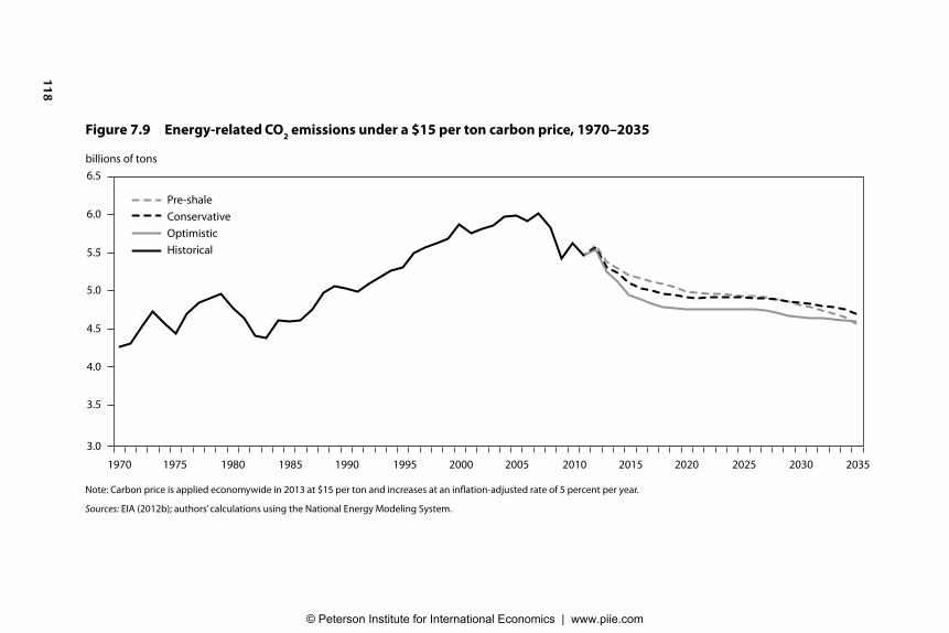
In our pre-shale scenario, a $15 per ton carbon price rising at an infla-tion-adjusted rate of 5 percent per year reduces annual CO2 emissions by 488 million tons per year in 2020 and 1,082 million tons per year in 2035 (figures 7.9 and 7.10 and table 7.2). That happens primarily through a shift from coal to nuclear and renewables in the power sector. In our optimistic scenario, low-cost natural gas provides a cheaper abatement opportunity and a carbon price extends and accelerates the recent coal-to-gas switch. CO2 emissions in 2020 are 225 million tons below where they would have been in a pre-shale world with the same carbon price, or 20.6 percent below 2005 levels as opposed to 16.8 percent. This is despite faster economic growth and energy demand in the optimistic scenario.

In the pre-shale scenario, a $15 per ton carbon price raises residential elec-tricity prices by 1.9 cents per kWh on average between 2013 and 2035 rela-tive to where they would have been without a carbon price in place (table 7.3). Because of low-cost natural gas, the increase in the optimistic scenario is only 1.6 cents per kWh. More importantly, US GDP is higher and household energy expenditures are lower in the optimistic scenario with a carbon price than in a pre-shale world without a carbon price. The US economy is $252 billion larger, on average, between 2013 and 2035 thanks to the increase in oil and gas production in the optimistic case. A $15 per ton carbon price would only offset a third of these gains and deliver important environmental cost savings as a result. Oil and natural gas prices would still be considerably lower with a carbon price than in a pre-shale world and residential electricity prices would be roughly the same.

On the producer side, the oil and gas boom makes a carbon price more attractive as well. In a pre-shale world, the most cost-effective pathway to reduce CO2 emissions was to switch from coal-fired power generation to renewables and nuclear (table 7.2 and figure 7.10). The political challenge of this solution was that, while the losers of such a policy were well known (e.g., coal producers and coal consumers), the winners had yet to be born (e.g., nuclear and renewable equipment manufacturers and installers). Take Texas as an example, which relies on coal shipped in from the Powder River Basin in Wyoming to generate a large share of its electricity. In a pre-shale world, pricing carbon would have raised the cost of electricity to the state’s residents with no assurance that the renewable or nuclear technology used to replace coal would be made by in-state companies. Given the number of states that rely on coal for power generation and their combined power in the US Senate, this kind of local economic math made passing climate legislation extremely difficult.

15. Our carbon price begins at $15 per ton in 2013 and rises at an inflation-adjusted rate of 5 percent per year through 2035.


118 Fu

eling

up

9

6.5

6.0

5.5

5.0

4.5

4.0

3.5

3.0

billions of tons

Figure 7.9 Energy-related CO2 emissions under a $15 per ton carbon price, 1970–2035

Note: Carbon price is applied economywide in 2013 at $15 per ton and increases at an inflation-adjusted rate of 5 percent per year.

Sources: EIA (2012b); authors’ calculations using the National Energy Modeling System.

2000 2005 2010 2015 2020 2025 2030 20351970 1975 1980 1985 1990 1995

Pre-shale

Conservative

Optimistic

Historical

zz--Figs_C

h7.indd 910/18/13 1:10 P

M © Peterson Institute for International Economics | www.piie.com


Figure 7.10 Power generation by source with a carbon price, 2011–35



4,500

4,000

3,500

3,000

2,500

2,000

1,500

1,000

500

0

5,000

20112012

20132014

20152016

20172018

20192020

20212022

20232024

20252026

20272028

20292030

20312032

20332034

2035

a. Pre-shale with carbon price


23

44

4,500

4,000

3,500

3,000

2,500

2,000

1,500

1,000

500

0

5,000

20112012

20132014

20152016

20172018

20192020

20212022

20232024

20252026

20272028

20292030

20312032

20332034

2035

b. Optimistic with carbon price


23

44

22

7

28

18

25

11

7

18

56

7

58

19

25

42

5

8

19

25

42

Coal Natural gasPetroleum NuclearHydro Other renewables

zz--Figs_Ch7.indd 10 11/8/13 8:57 AM


120 Fu

eling

up

16

Table 7.2 Combining a carbon price with the oil and gas boom

Source

Pre-shale Optimistic

2020 2035 2020 2035

Without CO2 price

With CO2 price

Without CO2 price

With CO2 price

Without CO2 price

With CO2 price

Without CO2 price

With CO2 price

Energy consumption Coal (million short tons) 1,085.0 828.7 1,237.0 687.6 763.5 434.6 865.0 274.8Oil (million barrels per day) 17.3 17.3 16.6 16.0 17.9 17.7 17.5 16.9Natural gas (trillion cubic feet) 22.9 22.8 21.6 21.6 29.8 31.5 32.9 35.9Nuclear (quadrillion British

thermal units)9.3 9.3 11.1 13.2 9.0 9.3 8.9 9.2

Renewables (quadrillion British thermal units)

10.4 12.3 15.7 21.9 10.3 10.8 14.5 16.4

Power generation (percent of total)Coal 43.6 34.5 43.1 24.9 29.5 16.2 28.1 7.0Oil 0.7 0.7 0.6 0.6 0.7 0.6 0.6 0.5Natural gas 19.9 22.9 16.6 17.6 35.7 46.1 40.1 56.1Nuclear 20.7 21.5 21.9 27.6 19.6 20.8 16.6 18.1Renewables 14.6 19.9 17.4 29.3 14.1 15.7 14.2 17.9

EnvironmentCO

2 emissions (energy-related,

billions of tons)5,475 4,987 5,646 4,564 5,326 4,762 5,668 4,594

SO2

emissions (power sector, millions of tons)

1.6 1.2 1.8 0.9 0.9 0.6 1.0 0.3

NOx emissions (power sector,

millions of tons)1.9 1.5 2.0 1.2 1.5 0.9 1.7 0.6

Mercury emissions (power sector, tons) 7.5 5.8 8.5 4.9 5.1 2.9 5.8 1.5



00--Tables.indd 16

11/7/13 12:13 PM © Peterson Institute for International Economics | www.piie.com

envir

on

men

tal C

osts a

nd

Ben

eFits 121 17

Table 7.3 Annual average producer revenue and consumer expenditures, 2013–35

Pre-shale Conservative Optimistic

Without

CO2 priceWith

CO2 priceWithout

CO2 priceWith

CO2 priceWithout

CO2 priceWith

CO2 price

Fossil fuel production Coal (million short tons) 1,186.10 882.20 1,096.70 770.00 895.00 523.50Oil (million barrels per day) 7.80 8.00 9.20 9.40 13.00 13.20Natural gas (trillion cubic feet) 21.60 21.10 25.70 26.50 31.30 32.90

Annual producer revenues (billions of 2010 US dollars)Coal 53.20 43.40 48.50 38.30 39.50 28.20Oil 376.20 381.80 429.30 425.00 529.20 526.70Natural gas 144.50 161.40 127.20 145.60 90.50 114.40

Energy prices and expenditures (2010 US dollars)Residential electricity prices (cents per kilowatt hour) 12.20 14.10 11.70 13.30 10.80 12.40Gasoline prices (US dollars per gallon) 3.90 4.10 3.80 4.00 3.50 3.70Natural gas prices (Henry Hub, US dollars per million British

thermal units)7.40 8.50 5.40 6.10 3.10 3.80

Average industrial energy price (US dollars per million British thermal units)

16.10 18.60 14.90 17.00 12.80 14.90

Household energy expenditures (2010 US dollars per household)

5,342.10 5,712.30 5,160.20 5,477.10 4,800.30 5,133.50

MacroeconomicGDP (trillions of 2005 chained US dollars) 18.79 18.73 18.87 18.79 19.04 18.96Employment (nonfarm, million people) 152.10 152.00 152.60 152.40 153.60 153.40



00--Tables.indd 17

11/7/13 12:13 PM


122 Fueling up

Coal consumption declines faster in the presence of a carbon price under either the conservative or optimistic scenario than in the pre-shale case, but natural gas makes up the difference instead of nuclear and renewables (table 7.2 and figure 7.10). This increase in natural gas demand raises prices. The combined effect is a 14 to 26 percent increase in natural gas production revenue on average between 2013 and 2035 (table 7.3). Domestic oil produc-tion actually increases with a carbon price—between 148,000 and 175,000 barrels per day (bbl/d)—as more CO2 is available for enhanced oil recovery. On the whole, oil and gas producer revenue increases by $14.2 billion to $21.4 billion per year between 2013 and 2035. Coal producer revenue declines by between $10.2 billion and $11.3 billion per year—leaving fossil fuel producers as a group better off with a carbon price than without. This potentially changes the political math of climate change policy. In a post-shale world, a carbon price moves Texas and a number of other states away from coal mined elsewhere in the country to natural gas produced in their own backyard. This, along with a smaller electricity price increase thanks to low-cost natural gas, could potentially make pricing carbon (either through legislation or regula-tion) more politically attractive in gas-rich parts of the country. And as the shale boom has spread, gas-producing states are increasingly outnumbering coal-producing states. Even in Pennsylvania, a long-time coal powerhouse, more people are employed in the oil and gas industry.

While low-cost natural gas makes reducing CO2 emissions cheaper and more politically attractive in the short and medium term, achieving the long-term emission reductions required to address climate change will require moving from natural gas to nuclear and renewables, or equipping natural gas-fired power plants with carbon capture and sequestration.16 The problem is that on a cost basis alone, nuclear and renewables will have a difficult time competing with natural gas over the next decade. Lower renewable and nuclear deployment in the short and medium term means higher costs in the long term, making future mitigation more difficult. Policymakers can address this by using some of the tax revenue generated through higher oil and gas royalty and lease revenue, or hypothetically carbon tax revenue were such legislation to pass, to fund nuclear and renewable research, development, and deploy-ment and help foster further progress in these technologies.

16. See, for example, Michael A. Levi, 2012, “The Climate Change Limits of U.S. Natural Gas,” Council on Foreign Relations, August 20, 2012, http://blogs.cfr.org/levi/2012/08/20/the-climate-change-limits-of-u-s-natural-gas.


environmental costs and benefits - piie · 2014. 1. 3. · shale gas drilling sites (mckenzie et...

Documents