ENVIRONMENTAL CHANGE IN THE EASTERN TROPICAL PACIFIC OCEAN:

OBSERVATIONS IN 1986-1990 AND 1998-2000

Paul C. Fiedler and Valerie A. Philbrick

Southwest Fisheries Science Center National Marine Fisheries Service, NOAA

8604 La Jolla Shores Drive La Jolla, California 92037

JUNE 2002

ADMINISTRATIVE REPORT LJ-02-15

ABSTRACT

Physical and biological oceanographic data have been collected on NOAA

dolphin surveys in the eastern tropical Pacific since the late 1970’s. We present yearly means and fields of surface temperature, thermocline depth, and surface chlorophyll for surveys in 1986, 1987, 1988, 1989, 1990, 1998, 1999, and 2000 to examine variability between years and between survey periods of 1986-1990 and 1998-2000. Yearly spatial patterns consistently show cooler surface temperature, more shallow thermocline and enhanced productivity in equatorial and coastal regions, compared to the eastern Pacific warm pool region in the central core of the survey area. Regional effects of El Niño and La Niña are clearly visible in changes between yearly observed fields, but there are no significant differences between 1986-1990 and 1998-2000. Primary productivity and zooplankton results for 1998-2000 are compared to historical data, but no conclusions can be made about change or lack of change of these variables.

INTRODUCTION

The eastern tropical Pacific Ocean (ETP) has been surveyed since 1974 by the Southwest Fisheries Science Center of the U. S. National Marine Fisheries Service, primarily to estimate the abundance of dolphin stocks. Monitoring of Porpoise Stocks (MOPS) surveys were conducted in 1986-1990 and Stenella Abundance Research (STAR) surveys were conducted in 1998-2000. Oceanographic data were collected as possible, within the constraints of the line transect survey, for several purposes: 1) to help interpret changes in stock abundance estimates, 2) to advance knowledge of stock distribution and ecology, 3) to monitor interannual change in the study area, and 4) to contribute to ongoing U.S. and international programs investigating oceanography and ocean-atmosphere interactions in the ETP. Constraints imposed by the priority of the line transect survey operations were that only limited underway sampling was possible during daylight dolphin survey effort and that samples had to be collected as time permitted along a trackline that was not necessarily optimal for oceanographic sampling.

Despite these operational constraints, data that are useful for all the above objectives have been collected. For example, Fiedler et al. (1992) analyzed variability of the thermocline and primary production related to the El Niño/Southern Oscillation (ENSO), Fiedler et al. (1991) showed how primary productivity is related to oceanic upwelling, Reilly and Fiedler (1994) found distinct environmental preferences for important dolphin stocks, and Ballance et al. (1997) demonstrated that seabird communities are organized along an environmental gradient. In this report, we present oceanographic results from annual dolphin surveys conducted in 1986-1990 and 1998-2000 and analyze environmental variability between years and decades (late 1980’s and late 1990’s) within the large survey area. Data from other sources (NCEP temperature and EASTROPAC zooplankton volumes, see below) are used to supplement survey data in assessing environmental change.

An independent scientific peer review of this work was administered by the Center for Independent Experts located at the University of Miami. Responses to reviewer’s comments can be found in Appendix A.

1

MATERIALS AND METHODS

All ETP dolphin surveys began on about July 28 and ended on about December 9, from San Diego, California. Therefore, data were collected almost entirely during the months of August-November. Two NOAA ships were used in all years, the David Starr Jordan and McArthur. A third ship, the University of Rhode Island’s Endeavor, was used in 1998. Oceanographic data collection during MOPS and STAR surveys followed standard methodologies throughout the fifteen years of effort, although instrumentation upgrades did occur. All station sampling was done in the early morning or evening. Only underway sampling was done during daytime sighting effort. Methods are summarized here; details may be found in MOPS and STAR data reports1.

Temperature and salinity of surface water were measured continuously and recorded in digital form on a PC at 2-minute intervals, or digitized from a strip chart (1986). Surface seawater was sampled from an intake 3 meters below the surface. Discrete bucket temperatures and salinity samples were collected at regular intervals to verify thermosalinograph readings.

Expendable bathythermograph (XBT) drops, to 760 meters depth, were made daily at three times (mid-morning, noon, and mid-afternoon) and also at midnight on MOPS cruises. Conductivity, temperature and depth (CTD) casts were made each morning before sunrise and each evening after sunset. The CTD was lowered to 1000 meters and sensors connected to shipboard computers measured conductivity (salinity), temperature and pressure (depth). Water samples were collected on all CTD casts with a 12-bottle rosette, for salinity calibration, nutrient and phytoplankton pigment analysis. Samples for 14C-uptake incubations were taken from morning casts starting in 1990. Samples (275 ml) from #200 meters were collected for phytoplankton pigment analysis at each station. Additional surface chlorophyll samples were collected by bucket at the same time as XBT deployment, or every two hours on some cruises. Extracted chlorophyll a and phaeophytin were measured by the standard fluorometric method on board ship. Nutrient samples (20 ml) for post-cruise analyses of nitrate, nitrite, phosphate and silicate were collected to #500m and immediately frozen after each cast. STAR nutrient samples have not been analyzed; no nutrient results will be presented here. At least two salinity samples (typically from 500m and 1000m) were collected on each cast and analyzed on board the ship for CTD calibration. Primary productivity by 14C uptake was measured by simulated in situ incubation of morning CTD samples from standard light levels estimated from historical data, using semi-clean techniques and 24-hour incubations. These data were not collected prior to 1990 and are not considered critical to dolphin habitat assessment. Phytoplankton pigment concentration is a fairly good index of primary productivity in this iron-limited system (Barber and Chavez, 1991). However, these results are presented here because open ocean measurements of primary productivity are rarely done repeatedly over such large areas. Acoustic backscatter data were collected underway on some surveys. 38-kHz data have been interpreted as an index of micronekton prey availability (Fiedler et al., 1998). 1 Available on request from Valerie.Philbrick@noaa.gov. STAR reports at http://swfsc.nmfs.noaa.gov /mmd/ecology/projects/etp.html

2

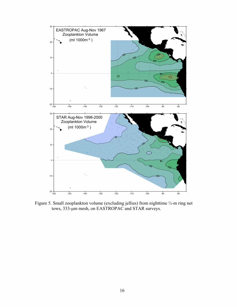
However, no valid acoustic backscatter data were collected during MOPS years, due to various hardware development problems, so these results are not presented here. Macrozooplankton net samples were collected on STAR surveys, but not on MOPS surveys due to logistical and time constraints. On all STAR surveys, when time permitted, a Bongo net was towed obliquely from 200 meters depth for 15 minutes two to three hours after sunset. The Bongo is a paired zooplankton net frame with two 333-µm mesh nets, fitted with a flowmeter in the outboard side. A sample was collected only from the outboard net, preserved in 5% buffered formalin, then labeled and stored for post-cruise analysis. On some STAR cruises in 1998 and 1999, a ½-meter ring net, with 333-µm mesh, was towed obliquely from 200 meters depth for 15 minutes.

Bongo nets are more efficient samplers of zooplankton than are ring nets, due to lower avoidance (Ohman and Smith, 1995). In 86 sets of paired net tows (one immediately following the other) during 1998 and 1999, the mean ratio of ring net plankton volume to Bongo net plankton volume was 0.43 ±0.19. Therefore, Bongo net plankton volumes were converted to ring net equivalent plankton volumes using a factor of 0.43. The ½-meter ring net was intended to replicate the EASTROPAC macrozooplankton net, which was a 333-µm mesh net on ½-meter ring attached to a large frame that also held a 1-meter ichthyoplankton net (Blackburn et al., 1970). However, the ring net and the EASTROPAC net were not ideal replicates, because of probable but unknown differences in tow speed and trajectory. The EASTROPAC net was towed at 1.5-2 knots to maintain the nominal wire angle of 45° (Blackburn et al., 1970), while the Bongo net on STAR was typically towed at 1-1.5 knots. In three sets of ring and Bongo tows on STAR 1999, with a time-depth recorder attached to the wire above the net, the Bongo net fished shallower and in a more irregular trajectory than the ring net. Neither net reached the nominal 200-m maximum depth in these three trials. In 88 net tows with a mechanical depth gauge on EASTROPAC, the measured maximum depth was less than the estimated depth in 84% of the tows, and the estimated depth ranged from 75-254 meters (Blackburn et al., 1970). Yearly fields of surface temperature, thermocline depth, surface chlorophyll, and primary productivity are presented and compared here. Zooplankton net samples were not collected on MOPS. During STAR, zooplankton samples were collected when time permitted east of 120°W. Therefore, a mean field of equivalent (see above) zooplankton volume for STAR (Aug-Nov 1998-2000) is compared to a field of zooplankton volume from EASTROPAC samples collected in August-November 1967 (NOAA/National Oceanographic Data Center). However, despite the steps taken to reconcile the STAR and EASTROPAC zooplankton sampling, we do not believe the data sets can be quantitatively compared with confidence. For the temperature variables, we averaged August through November monthly or weekly Pacific Ocean hindcast data fields produced by NCEP (NOAA/NWS National Center for Environmental Prediction; Behringer et al., 1998). NCEP uses a dynamic ocean model, driven by observed wind stress and surface heat fluxes, to assimilate sparse temperature observations, including CTD and XBT data collected on MOPS and STAR cruises and submitted to NODC. The observations constrain the model, while at the same time the model interpolates across data gaps using the physics of the model ocean. The NCEP hindcast grids have a resolution of 1-degree latitude and 1.5-degree longitude.

3

Surface chlorophyll, primary productivity, and zooplankton volume were gridded at a resolution of 1-degree latitude and longitude, using kriging routines in SURFER. Neither the NCEP nor the observed gridded fields for the August-November survey periods resolve short-lived mesoscale features. These mean fields are intended to show large-scale patterns and interannual differences only. The effect of averaging is reduced somewhat because August-November covers a seasonal extreme when southeast trade winds are strong along the equator, resulting in strong equatorial upwelling and cold surface temperatures in the equatorial cold tongue, and the intertropical convergence zone is at its northern extreme, resulting in low wind mixing and warm surface temperatures in the eastern Pacific warm pool. The fit between CTD and XBT observations and the August-November NCEP fields for the three STAR years was high for surface temperature (r2=0.89-0.91) and less for thermocline depth (r2=0.62-0.75). Thermocline depth was defined as the depth of the maximum temperature gradient over a depth interval of 15m, calculated from observed CTD or XBT profiles of ~1m resolution or from a 1-m spline interpolation of NCEP temperature profiles (defined at model depths of 5, 15, 25, 35, 45, 55, 65, 75, 85, 95, 106.25, 120, 136.25, 155, 177.5, 205, 240, 285, 345, 430, 550, and 720 m). Variability between years and between decades (i.e. between MOPS and STAR periods), was measured by statistical analysis of the gridded values within a survey area enclosed by both the MOPS and STAR survey boundaries and within a core area in the center of the survey area (5-20°N, east of 120°W). The core area corresponds to the region of warmest subtropical surface water in the ETP (Wyrtki, 1966), known as the eastern Pacific warm pool, and covers the ranges of two important dolphin stocks. Survey area and core area boundaries can be seen in Figs. 1-4. To separate temporal variability between decades from spatial variability within the areas, an unbalanced two-way analysis of variance was done on means of gridded variables in 5-degree squares using STATISTICA. In this 2 x 56 (or 2 x 16 for the core area) ANOVA design, error variance was the variance between the five MOPS years and the three STAR years. Gridded values, rather than observed values, were used for statistical analyses because the data points were not randomly or systematically distributed (Figs. 3, 4).

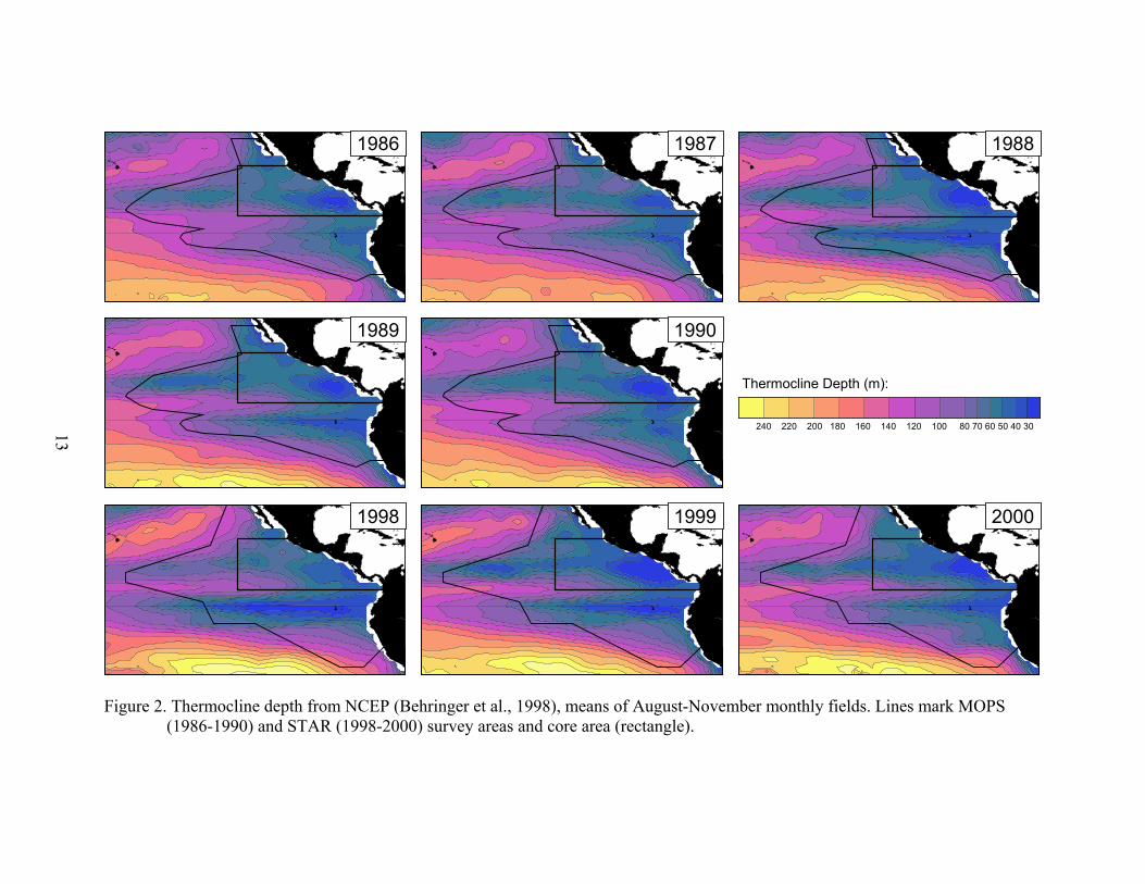
RESULTS Surface temperature fields (Fig. 1) showed the expected summer/fall pattern: a cold tongue extending from Ecuador across the survey area, slightly south of the equator; the eastern Pacific warm pool north of the cold tongue and east of 120°W (in the core area); and cold water in the California Current along southern Baja California and in the Humboldt Current along Peru. Thermocline depth fields (Fig. 2) showed the zonal pattern of thermocline ridging associated with the equatorial current system: the equatorial thermocline ridge along the equator and the countercurrent thermocline ridge along 10°N. In addition to this zonal ridging, the thermocline deepens from east to west. The themocline was deepest in the subtropical gyres of the North and South Pacific, to the northwest and southwest of the survey area. Effects of the 1986-87 El Niño included a less pronounced cold tongue in 1986 and 1987, and a warmer warm pool in 1987, with 28°C water extending west out of the core area and across the entire survey area. The equatorial thermocline ridge deepened

4

during this event, and was actually deeper in 1986 than in 1987. The strong 1997-98 El Niño abated from its mature phase in November-December 1997 to near-normal SST’s in the eastern equatorial Pacific by July 1998 (Enfield, 2001). Lingering effects were evident during STAR 1998 in the core area, where surface water was a few tenths of a degree warmer and the thermocline a few meters deeper than in 1999 and 2000, when weak La Niña conditions prevailed. Biological effects of El Niño and La Niña, or ENSO variability, were evident in the surface chlorophyll fields (Fig. 3). Chlorophyll levels were low in 1987, the expected result of the deeper thermocline/nutricline and reduced wind mixing. Chlorophyll levels along the equator and along the coast in the core area were elevated during La Niña 1988. During STAR 1998, low chlorophyll levels in the core area were probably a lingering effect of El Niño 1997-1998. STAR sea surface temperature, thermocline depth, and surface chlorophyll fields were within the range observed during MOPS, when a moderate ENSO cycle occurred. The primary productivity fields (Fig. 4) showed large-scale patterns very similar to the chlorophyll fields. High productivity occurred consistently near the coast of Peru and along the equator. In some years, high productivity also occurred in coastal waters of Central America and Baja California. The zooplankton volume fields (Fig. 5) showed higher zooplankton biomass along the equator, increasing to the east, and off Central America at about 10°N. STAR (1998-2000) zooplankton volumes are not mapped by year because yearly sample coverage was not consistent. Time series of 1980-2001 yearly (August-November) mean sea surface temperature and thermocline depth showed interannual variability related to ENSO both in the survey area as a whole and in the core area (Fig. 6). El Niño periods (1982-1983, 1986-1987, 1997-1998) were characterized by anomalously warm surface temperatures and deep thermoclines. La Niña periods (1984-1985, 1988-1989, 1999-2000) were characterized by anomalously cool surface temperatures and shallow thermoclines. The warming and thermocline deepening in August-November 1997 were much greater than in August-November 1982, probably because the 1997-98 El Niño matured several months earlier than the 1982-83 El Niño and peaked during the August-November 1997 period (Enfield, 2001). Mean surface chlorophyll values showed the 1987 reduction and 1988 enrichment seen in the yearly fields (Fig. 3). 1998-2000 surface chlorophyll levels were all close to the mean of the eight MOPS/STAR years. The primary productivity results showed an apparent increase in levels between MOPS 1990 and STAR, at least for the survey area as a whole. However, problems in estimating total levels of activity in 1990 forced us to use a nominal value, which resulted in a negative bias in the estimated productivity values (Fiedler et al., 1992). Therefore, the difference in ETP primary productivity between 1990 and the late 1990’s was most likely an artifact. The error bars in the yearly time series (Fig. 6) are standard deviations of the gridded anomaly values. Spatial autocorrelation of the gridded values likely reduces the degrees of freedom to about 0.1*n. ANOVA was carried out to remove the spatial variance (between 5° squares) from the variance between decades (Table 1). Sea surface temperature changed significantly in the survey area, and barely significantly within the core area. However, the change was only –0.27 °C. Neither thermocline depth, nor surface chlorophyll showed a significant change between decades. The significant

5

interaction effect for thermocline depth in the survey area suggests that significant regional changes occurred in areas other than the core area.

CONCLUSIONS Oceanographic data collected in the ETP during 1986-1990 and 1998-2000 clearly showed regional effects of ENSO variability. El Niño 1986-87 warmed surface waters, depressed the thermocline, and reduced phytoplankton biomass (surface chlorophyll) along the equator and in the core area (warm pool). La Niña 1988 cooled surface waters, raised the thermocline, and increased phytoplankton biomass. El Niño 1997-1998 had effects that lingered in the warm pool, but not along the equator, into the 1998 survey. Despite the year-to-year ENSO variability, or perhaps because of it, there were no observed changes between 1986-1990 and 1998-2000, except for a significant temperature difference of a few tenths of a degree C. A change of this magnitude may not be important in a region where sea surface temperature varies by several degrees between seasons and between years. Comparison between the two survey periods presented here does not accurately measure decadal variability. The five and three years of observations presented here are not adequate to resolve decadal scale variability, even when supplemented with 22 years of NCEP temperature data. Longer time series of some environmental variables are available and examined in Fiedler (2002), where ENSO and decadal scale environmental change, and resulting ecological effects, that might be expected in the eastern tropical Pacific are reviewed.

ACKNOWLEDGEMENTS We thank all the technicians and scientists who collected these data at sea, with the help of ships’ officers and crew, Robert Holland and Josh Fluty for assistance in data processing, Linda Stathoplos for providing the EASTROPAC zooplankton data, and Steve Reilly of SWFSC for continued support of marine mammal habitat studies. Several anonymous reviewers provided useful suggestions.

6

LITERATURE CITED Ballance, L. T., R. L. Pitman, and S. B. Reilly. 1997. Seabird community structure along

a productivity gradient: importance of competition and energetic constraint. Ecology 78:1502-1518.

Barber, R. T., and F. P. Chavez. 1991. Regulation of primary productivity rate in the

equatorial Pacific. Limnol. Oceanogr. 36:1803-1815. Behringer, D. W., M. Ji, and A. Leetmaa. 1998. An improved coupled model for ENSO

prediction and implications for ocean initialization. Part I: the ocean data assimilation system. Mon. Weath. Rev. 126:1013-1021.

Blackburn, M., R. M. Laurs, R. W. Owen, and B. Zeitzschel. 1970. Seasonal and areal

changes in standing stocks of phytoplankton, zooplankton and micronekton in the eastern tropical Pacific. Mar. Biol. 7:14-31.

Enfield, D. B. 2001. Evolution and historical perspective of the 1997-1998 El Niño-

Southern Oscillation event. Bull. Mar. Sci. 69:7-25.

Fiedler, P. C. 2002. Environmental change in the eastern tropical Pacific Ocean: Review of ENSO and decadal variability. Administrative Report No. LJ-02-16, NMFS, Southwest Fisheries Science Center, 8604 La Jolla Shores Drive, La Jolla, CA 92037.

Fiedler, P. C., J. Barlow, and T. Gerrodette. 1998. Dolphin prey abundance determined

from acoustic backscatter data in eastern Pacific surveys. Fish. Bull., U. S. 96:237-247.

Fiedler, P. C., F. P. Chavez, D. W. Behringer, and S. B. Reilly. 1992. Physical and

biological effects of Los Niños in the eastern tropical Pacific, 1986-1989. Deep-Sea Res. I 39:199-219.

Fiedler, P. C., V. Philbrick, and F. P. Chavez. 1991. Oceanic upwelling and productivity

in the eastern tropical Pacific. Limnol. Oceanogr. 36:1834-1850. Ohman, M. D., and P. E. Smith. 1995, A comparison of zooplankton sampling methods

in the CalCOFI time series. CalCOFI Rep. 36:153-158. Reilly, S. B., and P. C. Fiedler. 1994. Interannual variability of dolphin habitats in the

eastern tropical Pacific. I: Research vessel surveys, 1986-1990. Fish. Bull., U. S. 92:434-450.

Wyrtki, K. 1966. Oceanography of the eastern equatorial Pacific Ocean. Oceanogr. Mar.

Biol. Ann. Rev. 4: 33-68.

7

Survey Area Sea surface temperature

Thermocline depth

Surface chlorophyll

1986-1990 -0.13 °C -1.5 m +0.0065 mg m-3 Means 1998-2000 -0.40 °C -3.1 m +0.0080 mg m-3

Decade 0.0002*** 0.061 0.830 Space 1.000 0.018 * 1.000

ANOVA effects (P values) Interaction 1.000 0.0002*** 0.409

Core Area Sea surface temperature

Thermocline depth

Surface chlorophyll

1986-1990 -0.04 °C -2.0 m +0.0086 mg m-3 Means 1998-2000 -0.22 °C -2.2 m -0.0006 mg m-3

Decade 0.042* 0.850 0.354 Space 1.000 0.584 1.000

ANOVA effects (P values) Interaction 1.000 0.556 0.999

Table 1. Survey area and core area “decadal” means and effects of decade and space

(five-degree square) from ANOVA of gridded oceanographic anomalies observed during MOPS (1986-1990) and STAR (1998-2000) surveys. Chlorophyll was log-transformed before analysis of anomalies. *P<.05, ***P<.001.

11

12

1986 1987 1988

1989 1990

1998 1999 2000

16 17 18 19 20 21 22 23 24 25 26 27 28 29 30 31

Sea Surface Temperature (°C):

Figure 1. Sea surface temperature from NCEP (Behringer et al., 1998), means of August-November monthly fields. Lines mark MOPS (1986-1990) and STAR (1998-2000) survey areas and core area (rectangle).

13

1986 1987 1988

1989 1990

1998 1999 2000

240 220 200 180 160 140 120 100 80 70 60 50 40 30

Thermocline Depth (m):

Figure 2. Thermocline depth from NCEP (Behringer et al., 1998), means of August-November monthly fields. Lines mark MOPS (1986-1990) and STAR (1998-2000) survey areas and core area (rectangle).

14

MOPS 1986 MOPS 1987 MOPS 1988

MOPS 1989 MOPS 1990

STAR 1998 STAR 1999 STAR 2000

0.05 0.07 0.1 0.15 0.2 0.3 0.5 0.7 1.0 1.5 2 3

Surface Chlorophyll (mg m-3):

Figure 3. Surface chlorophyll from CTD casts and pump or bucket samples (+) on MOPS (1986-1990) and STAR (1998-2000) surveys. Rectangle marks core area.

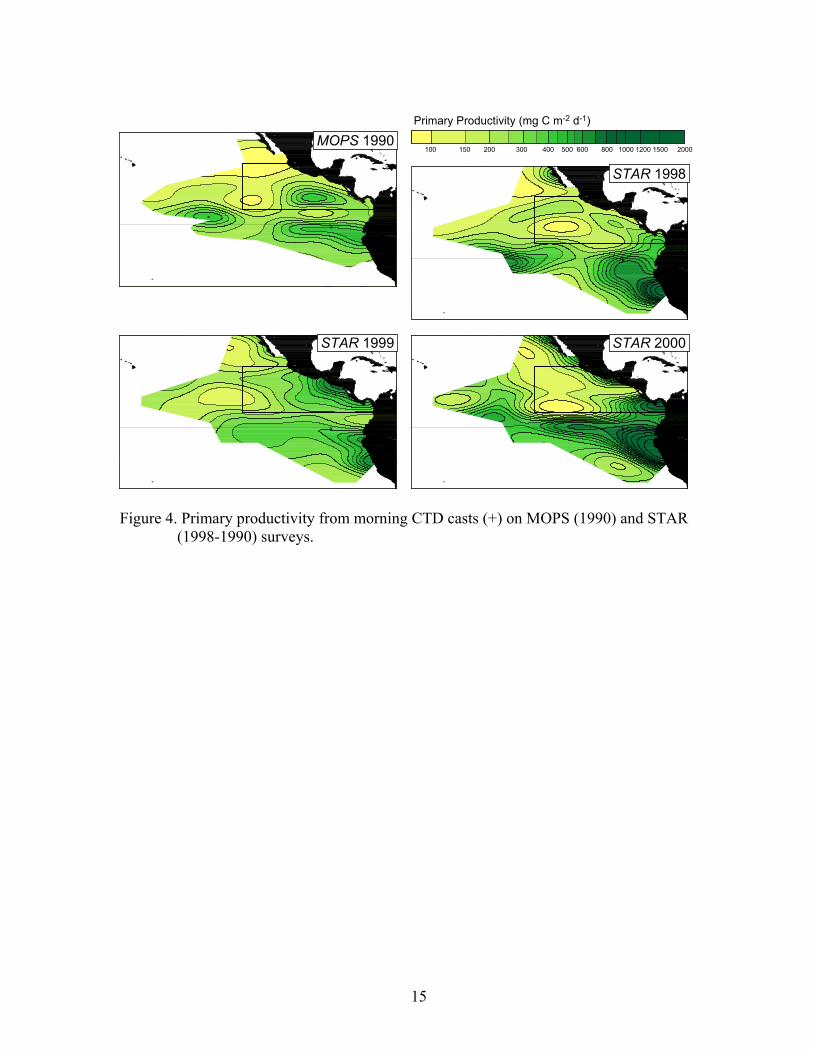
igure 4. Primary productivity from morning CTD casts (+) on MOPS (1990) and STAR

MOPS 1990

STAR 1998

STAR 1999 STAR 2000

Primary Productivity (mg C m-2 d-1)

100 150 200 300 400 500 600 800 1000 1200 1500 2000

F(1998-1990) surveys.

15

-160 -150 -140 -130 -120 -110 -100 -90 -80-20

-10

0

10

20

30

EASTROPAC Aug-Nov 1967Zooplankton Volume

(ml 1000m-3 )

-160 -150 -140 -130 -120 -110 -100 -90 -80-20

-10

0

10

20

30

STAR Aug-Nov 1998-2000Zooplankton Volume

(ml 1000m-3 )

Figure 5. Small zooplankton volume (excluding jellies) from nighttime ½-m ring net tows, 333-µm mesh, on EASTROPAC and STAR surveys.

16

-1

0

1

2

Sea

sur

face

tem

pera

ture

, °C

Survey Area Core Area

-15

-10

-5

0

5

10

15

Ther

moc

line

dept

h, m

-0.10

-0.05

0.00

0.05

0.10

Surfa

ce c

hlor

ophy

ll, m

g m

-3

1980 1985 1990 1995 2000-100

-50

0

50

100

Prim

ary

prod

uctiv

ity, m

g C

m-2

d-1

1980 1985 1990 1995 2000

ENSOevents

Figure 6. Mean August-November anomalies of gridded oceanographic variables in the study area (left) and core area (right). Error bars represent standard deviation of gridded anomaly values within the area. Surface chlorophyll and primary productivity were log-transformed. Dark bars are years of MOPS (1986-1990) and STAR (1998-2000) surveys. The “ENSO events” bar charts indicate periods when the monthly eastern equatorial surface temperature anomaly (NINO3) was >1°C (El Niño events, bar above axis) and <-1°C (La Niña events, bar below axis).

17

APPENDIX A Responses to CIE Reviewers The CIE reviewers provided useful comments on this document. General suggestions for future field work will be carefully considered. All suggestions specific to this report were incorporated in the final report, with exceptions detailed below. Ken Drinkwater Background information about “what earlier studies had concluded about the physical and biological variability of this ocean region” is included in the second oceanography paper reviewing environmental variability. Plots of primary productivity were retained because the spatial patterns are important. Quantitative analysis of correlation between SST and thermocline depth is not relevant to the objective of this report. The answer to “Are the increased chlorophyll levels just north of the equator related to the equatorial front?” is no, and the equatorial front has not been considered a factor in these studies for the reasons detailed by Ballance. Hazel Oxenford Methods for variables not presented here were left in the paper, because it is important to know what was attempted and what is available for future analyses.

18