environmental auditing assessing biotic integrity …dallan/pdfs/lammert_allan.pdf · relate...

ENVIRONMENTAL AUDITINGAssessing Biotic Integrity of Streams: Effects of Scalein Measuring the Influence of Land Use/Cover andHabitat Structure on Fish and MacroinvertebratesMARY LAMMERT*The Nature Conservancy8 S. Michigan Avenue, Suite 2301Chicago, Illinois 60603, USA

J. DAVID ALLANSchool of Natural Resources and EnvironmentThe University of MichiganAnn Arbor, Michigan 48109-1115, USA

ABSTRACT / Fish and macroinvertebrate assemblage com-position, instream habitat features and surrounding land usewere assessed in an agriculturally developed watershed torelate overall biotic condition to patterns of land use andchannel structure. Six 100-m reaches were sampled on eachof three first-order warm-water tributaries of the River Raisinin southeastern Michigan. Comparisons among sites andtributaries showed considerable variability in fish assem-blages measured with the index of biotic integrity, macroin-vertebrate assemblages characterized with several diversityindexes, and both quantitative and qualitative measure-

ments of instream habitat structure. Land use immediate tothe tributaries predicted biotic condition better than regionalland use, but was less important than local habitat variablesin explaining the variability observed in fish and macroinver-tebrate assemblages. Fish and macroinvertebrates ap-peared to respond differently to landscape configurationand habitat variables as well. Fish showed a stronger rela-tionship to flow variability and immediate land use, whilemacroinvertebrates correlated most strongly with dominantsubstrate. Although significant, the relationships betweeninstream habitat variables and immediate land use ex-plained only a modest amount of the variability observed. Aprior study of this watershed ascribed greater predictivepower to land use. In comparison to our study design, thisstudy covered a larger area, providing greater contrastamong subcatchments. Differences in outcomes suggeststhat the scale of investigation influences the strength of pre-dictive variables. Thus, we concluded that the importance oflocal habitat conditions is best revealed by comparisons atthe within-subcatchment scale.

Physical habitat is a primary factor influencing thestructure and composition of stream faunal communi-ties (Gorman and Karr 1978, Schlosser 1982, 1987,Frissell and others 1986, Angermeier 1987, Cummins1988, Osborne and Wiley 1992, Richards and others1993, Richards and Host 1994, Poff and Allan 1995).Recent work in ecology (Wiens 1989) and streamecology (Taylor and others 1993) has raised the ques-tion of the effect of scale in habitat investigations. Theparadigm that has emerged holds that environmentalvariability affecting stream organisms occurs at multiplespatial and temporal scales (Frissell and others 1986,Addicott and others 1987, Downes and others 1993,Taylor and others 1993, Townsend and Hildrew 1994).

Explicit recognition of scale is also a central concernof studies relating landscape structure to stream ecosys-tem processes (Hunsaker and Levine 1995). Accordingto the model of natural river systems by Frissell and

others (1986), stream systems are spatially nested hierar-chies of segments, reaches, pool/riffle units, and micro-habitats. The larger scale features constrain the develop-ment of smaller units, and the resulting physical patterns,across both spatial and temporal scales, strongly influ-ence the biology of the stream (Frissell and others 1986,Hawkins and others 1993, Rosgen 1994). However, thismodel, which links the physical structure of streams andtheir surrounding landscape to the distribution ofstream organisms, remains a largely untested hypothesis(Schlosser 1991).

The study described here explores the hierarchicalmodel of stream ecosystems by relating stream bioticintegrity to patterns of land use and instream habitat inthree agriculturally impacted streams. We sampled fishand macroinvertebrates and measured local habitatstructure and adjacent land use following several stud-ies that have sought to relate patterns of stream commu-nity composition to specific instream habitat and land-scape features (Schlosser 1982, 1985, 1987, Steedman1988, Wiley and others 1990, Osborne and Wiley 1992,Richards and others 1993, Malmqvist and Maki 1994,

KEY WORDS: Stream; Biomonitoring; Land use; Scale; Habitat; Fish;Macroinvertebrates

*Author to whom correspondence should be addressed.

Environmental Management Vol. 23, No. 2, pp. 257–270 r 1999 Springer-Verlag New York Inc.

Richards and Host 1994, Roth and others 1996). Wefocused on agricultural impacts because agriculture hascaused extensive landscape changes (Allan 1995). Dif-fuse nutrient and sediment pollution from agriculturehas been identified as the leading cause of water qualitydegradation in the United States (Osborne and Kovacic1993).

Biotic indexes were used to measure biotic integrityfor this study. Declines in stream ecosystems despiteimprovements in water quality associated with implemen-tation of the Clean Water Act (33 U.S.C. 1251–1387)have spurred development of biological measures ofwater quality based on attributes of fish and macroinver-tebrate communities (Karr and others 1986, Plafkinand others 1989, Quinn and Hickey 1990, Osborne andothers 1991, Meador and others 1993, Rosenberg andResh 1993, Kerans and Karr 1994). The faunal composi-tion of streams is thought to reflect ambient conditionsand integrate the influences of water quality and habitatdegradation (Meador and others 1993).

Fish and macroinvertebrate indexes measure faunaldiversity, functional diversity, and pollution toleranceand are used to rate sites against reference conditionsfor same sized streams within an ecoregion. However,these two taxonomic groups offer different advantagesas water quality indicators. The multimetric index ofbiotic integrity (IBI) comprises fish species richness,dominance, abundance, trophic structure, tolerance todegraded conditions, and individual health (Karr andothers 1986). Two principal advantages of using the IBIare its widespread use and the availability of referencedata on fish. Macroinvertebrates are ubiquitous tostreams and often exhibit greater taxonomic and tro-phic variety than fish. Plafkin and others (1989) suggestthat macroinvertebrates are more indicative of localhabitat conditions while fish reflect conditions overbroader spatial areas because of their relative mobilityand longevity.

Little agreement exists, however, about how to de-scribe macroinvertebrate assemblages for biologicalassessment (Rosenberg and Resh 1993). An indexcomparable to the IBI has been developed for macroin-vertebrates (Kerans and Karr 1994), but this index, thebenthic index of biotic integrity (B-IBI), has yet to beapplied widely. Other indexes that have been usedwidely include the invertebrate community index (ICI)(Ohio EPA 1988), which is similar to the B-IBI, and thebiotic index (BI), which is based on pollution toler-ances (Hilsenhoff 1987).

Our first objective was to test the hypothesis thatdifferences in land use among catchments account fordifferences in biotic integrity among the streams ofthose catchments. Our second objective was to analyze

the effect of local habitat variation on the relationshipbetween land use and stream biota. The third objectivewas to compare the information generated by fish andmacroinvertebrate assemblage measures, both in termsof their ability to distinguish or rank site quality and todetermine if fish and macroinvertebrates respondedsimilarly to instream habitat and landscape features.

Methods

Study Reach

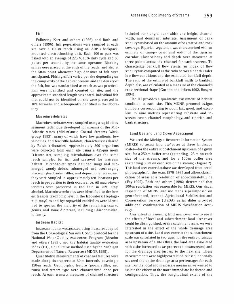
The study area lies within the River Raisin watershed,a 2776 km2 drainage basin located in southeasternMichigan, USA. Surficial geology is primarily fine-textured end moraine with coarse-grained end moraineand outwash deposits interspersed in the upper basinand fine-textured glacial lake deposits in the lowerbasin. Our study sites were within morainal regions(Figure 1), which minimized the differences in geologyamong sites, although some local variation was evident.Land use within the River Raisin watershed is predomi-nantly agriculture, but varies among subcatchments. Weselected three tributaries, Iron, Evans, and Hazen creeks,which represent subcatchments with differing amountsof agriculture. Six sites on each tributary were systemati-cally spaced to cover the entire length of the tributary ina balanced one-way analysis of variance (ANOVA) de-sign.

Based on visual inspection and our subjective impres-sions, we expected Iron Creek to contain more forestedland and to have sites of higher quality than eitherEvans or Hazen creeks. Evans Creek is known to havebeen channelized, and Hazen Creek appeared stronglyimpacted by surrounding agricultural activity. We usedthe land use/cover classification system developed bythe Michigan Department of Natural Resources todescribe the three subcatchments in terms of sevenmajor land use/cover categories: urban/extractive/open miscellaneous, agricultural, rangeland, forested,water, wetland, and barren. The agriculture categoryincludes cropland, orchards, confined feed operations,and permanent pasture. Rangeland is either herba-ceous vegetation or shrubland. The catchment areas ofIron Creek, Evans Creek, and Hazen Creek are 51.7km2, 49.8 km2, and 75.5 km2, respectively. The predomi-nant land use/cover types in all three catchments areagricultural land, forested land, and rangeland. To-gether these three categories account for 81% of IronCreek’s catchment, 88% of Evans Creek’s, and 96% ofHazen Creek’s. Urban land use is low throughout thebasins of all three tributaries, accounting for only 1% ofthe Hazen Creek drainage area, 7% of Iron Creek’s, and9% of Evans Creek’s.

M. Lammert and J. D. Allan258

Fish

Following Karr and others (1986) and Roth andothers (1996), fish populations were sampled at eachsite over a 100-m reach using an ABP-3 backpack-mounted electroshocking unit. Each 100-m pass wasfished with an average of 225 V, 10% duty cycle and 60pulses per second, by the same operator. Blockingseines were placed at the ends of the reach, and also atthe 50-m point whenever high densities of fish wereanticipated. Fishing effort varied per site depending onthe complexity of the habitat present and the density ofthe fish, but was standardized as much as was practical.Fish were identified and counted on site, and theapproximate standard length was noted. Individual fishthat could not be identified on site were preserved in10% formalin and subsequently identified in the labora-tory.

Macroinvertebrates

Macroinvertebrates were sampled using a rapid bioas-sessment technique developed for streams of the Mid-Atlantic states (Mid-Atlantic Coastal Streams Work-group 1993), many of which have low gradients, lowvelocities, and few riffle habitats, characteristics sharedby Raisin tributaries. Approximately 300 organismswere collected from each site using a 425-µm meshD-frame net, sampling microhabitats over the samereach sampled for fish and surveyed for instreamhabitat. Microhabitat types included snags and sub-merged woody debris, submerged and overhangingmacrophytes, banks, riffles, and depositional areas, andthey were sampled in approximately ten locations perreach in proportion to their occurrence. All macroinver-tebrates were preserved in the field in 70% ethylalcohol. Macroinvertebrates were identified to the low-est feasible taxonomic level in the laboratory. Heptage-niid mayflies and hydropsychid caddisflies were identi-fied to species, the majority of the remaining taxa togenus, and some dipterans, including Chironomidae,to family.

Instream Habitat

Instream habitat was assessed using measures adaptedfrom the US Geological Survey (USGS) protocol for theNational Water-Quality Assessment Program (Meadorand others 1993), and the habitat quality evaluationindex (HI), a qualitative method used by the MichiganDepartment of Natural Resources (MDNR 1989).

Quantitative measurements of channel features weremade along six transects at 30-m intervals, covering a150-m reach. Geomorphic feature (pools, riffles, andruns) and stream type were characterized once perreach. At each transect measures of channel structure

included bank angle, bank width and height, channelwidth, and dominant substrate. Assessment of bankstability was based on the amount of vegetative and rockcoverage. Riparian vegetation was characterized with anestimate of canopy cover and width of the ripariancorridor. Flow velocity and depth were measured atthree points across the channel for each transect. Tocharacterize bankfull flow events, an index of flowstability was computed as the ratio between depth underlow flow conditions and the estimated bankfull depth.The ratio of the estimated bankfull width to bankfulldepth also was calculated as a measure of the channel’scross sectional shape (Gordon and others 1992, Rosgen1994).

The HI provides a qualitative assessment of habitatcondition at each site. This MDNR protocol assignsnumbers corresponding to poor, fair, good, and excel-lent to nine metrics representing substrate and in-stream cover, channel morphology, and riparian andbank structure.

Land Use and Land Cover Assessment

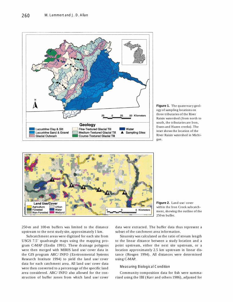
We used the Michigan Resource Information System(MIRIS) to assess land use/cover at three landscapescales—for the entire subcatchment upstream of a givensite, for a 250-m buffer area (extending 125 m on eachside of the stream), and for a 100-m buffer area(extending 50 m on each side of the stream) (Figure 2).This land use/cover database was developed from aerialphotographs for the years 1979–1985 and allows classifi-cation of areas at a resolution of approximately 1 ha(Fay 1995). Roth and others (1996) determined that100-m resolution was reasonable for MIRIS. Our visualinspection of MIRIS land use maps superimposed ongeoreferenced, scanned Agricultural Stabilization andConservation Service (USDA) aerial slides providedadditional confirmation of MIRIS classification accu-racy.

Our intent in assessing land use/cover was to see ifthe effects of local and subcatchment land use/covercould be distinguished. At the catchment scale, we wereinterested in the effect of the whole drainage areaupstream of a site. Land use/cover at the subcatchmentscale was calculated in two ways: for the entire drainagearea upstream of a site (thus, the land area associatedwith a site increased as we proceeded downstream) andfor the drainage area just up to the next site. Thesemeasurements were highly correlated: subsequent analy-ses used the entire drainage area percentages for eachsite. For the local and mesoscale measures, we wanted toisolate the effects of the more immediate landscape andconfiguration. Thus, the longitudinal extent of the

Assessing Biotic Integrity of Streams 259

250-m and 100-m buffers was limited to the distanceupstream to the next study site, approximately 1 km.

Subcatchment areas were digitized for each site fromUSGS 7.58 quadrangle maps using the mapping pro-gram C-MAP (Enslin 1991). These drainage polygonswere then merged with MIRIS land use/cover data inthe GIS program ARC/INFO (Environmental SystemsResearch Institute 1994) to yield the land use/coverdata for each catchment area. All land use/cover datawere then converted to a percentage of the specific landarea considered. ARC/INFO also allowed for the con-struction of buffer zones from which land use/cover

data were extracted. The buffer data thus represent asubset of the catchment area information.

Sinuosity was calculated as the ratio of stream lengthto the linear distance between a study location and apoint upstream, either the next site upstream, or alocation approximately 2.5 km upstream in linear dis-tance (Rosgen 1994). All distances were determinedusing C-MAP.

Measuring Biological Condition

Community composition data for fish were summa-rized using the IBI (Karr and others 1986), adjusted for

Figure 1. The quaternary geol-ogy of sampling locations onthree tributaries of the RiverRaisin watershed (from north tosouth, the tributaries are Iron,Evans and Hazen creeks). Theinset shows the location of theRiver Raisin watershed in Michi-gan.

Figure 2. Land use/coverwithin the Iron Creek subcatch-ment, showing the outline of the250-m buffer.


the River Raisin following Roth and others (1996) andMDNR (1989). Multiple indexes were available to char-acterize macroinvertebrate communities. Resh and Jack-son (1993) argue against relying on a single measure;thus, we used two multimetric indexes, the B-IBI andthe ICI, four single-value metrics (taxa richness, taxaevenness, sensitive taxa richness, and number of mayflytaxa), and the BI, which is based on organic pollutiontolerance. Calculation of the B-IBI, originally developedfor streams in the Tennessee Valley drainage (Keransand Karr 1994), required modification for use insoutheastern Michigan to account for taxonomic differ-ences. Four of the 13 metrics were eliminated and thescoring criteria were adjusted by trisecting the range ofvalues obtained in this study and assigning scores of 1(poor), 3, and 5 (best observed condition) (Table 1).The ICI uses a scoring system scaled to the drainagearea for all of the metrics except percent mayflycomposition and the percent tribe Tanytarsini midgecomposition, and assigns a score of 0 (worst condition),2, 4, or 6 (best condition) (Ohio EPA 1988). Due todifferences in taxonomic identification level, metricsfor presence of tolerant species and for the presence ofTanytarsini midges were omitted. Taxa evenness wascalculated using Shannon’s index (Shannon 1948). The

remaining single-value indexes are self-evident, exceptfor sensitive taxa richness, which refers to the numberof Ephemeroptera, Plecoptera, and Trichoptera (EPT)taxa.

Biotic index scores were determined according tothe procedures described by Hilsenhoff (1987) andLenat (1993). Tolerance values were assigned to thetaxa based on the values given in Lenat (1993) or inHilsenhoff (1987, 1988) where Lenat (1993) offered novalue. The number of individuals in each taxonomicgroup was multiplied by its tolerance value, and aweighted average tolerance score for that sample wascalculated (Hilsenhoff 1987). A higher score indicates amore degraded site in terms of organic pollution but isnot necessarily an indicator of habitat degradation.

Results

Fish

Over 3000 fish were collected from the 18 sites. Sixfish species accounted for 75% of the individualscaptured, with the creek chub (Semotilus atromaculatus)being the most abundant and ubiquitous fish, found at17 of 18 sites. Other commonly occurring speciesincluded blacknose dace (Rhinichthys atratulus), stone-roller (Campostoma anomalum), mottled sculpin (Cottusbairdi), white sucker (Catostomus commersoni), and johnnydarter (Etheostoma nigrum). Rare species, those thatcomprised less than 1% of the total catch, accounted for14 of the 28 species collected (see Lammert 1995 for afull list). Fish abundance varied considerably amongsites, ranging from a low of six individuals to a high of769, with a mean of 174 fish per site. The density of fishvaried from 0.04 to 1.42 fish/m2 (Figure 3A). Sites onEvans Creek generally had the lowest abundance, spe-cies richness, and densities. Although Iron Creek hadlower average fish abundance than Hazen Creek, thetwo streams had similar average species richness.

IBI scores varied among sites from a high of 42 of apossible 50 points at two upper Iron Creek sites to a lowof 14 at one mid-stream site on Evans Creek (overallmean 6 SD; 31.7 6 8.7; Figure 3B). Scores from EvansCreek sites were significantly lower than those of Ironand Hazen creeks (F 5 11.6, df 5 2, P 5 0.001), butIron and Hazen creeks were not significantly different(Tukey P 5 0.425).

We were interested in which metrics contributedmost significantly to the IBI scores. Using multiplelinear regression, we determined that a two-metricmodel explained over 85% of the score value. Speciesrichness was most highly correlated to the total IBIscore (R 5 0.822). Of the remaining metrics, onlypercent insectivorous fish and the number of intoler-

Table 1. Metrics and scores for the benthic indexof biotic integrity (B-IBI) metricsa

Metric

Score

1 3 5

Total taxa (Intolerantsnail and musselrichness) 14–22 23–30 30–39

Mayfly taxa 0–3 4–6 7–9Caddisfly taxa 2–3 4–5 6–7Dipteran taxa (Stonefly

taxa) 3–4 5–6 7–8

(Relative abundance ofCorbicula sp.)

(Relative abundance ofoligochaetes)

Relative abundance ofomnivores 0.70–0.81 0.57–0.69 0.43–0.56

Relative abundance offilterers 0.51–0.69 0.50–0.31 0.09–0.30

Relative abundance ofgrazers 0.06–0.19 0.20–0.32 .0.33

Relative abundance ofpredators 0.24–0.33 0.14–0.23 0.02–0.13

Dominance (Totalabundance) 0.68–0.88 0.47–0.67 0.24–46

aModified from Kerans and Karr (1994). The description of eachmetric appears in the left column and the scoring criteria to the right.Metrics omitted from this study are enclosed in parentheses.


ants (individuals of species considered intolerant tosiltation and pollution) were significantly correlated tothe residuals of the regression between species richnessand total score. The addition of percent insectivorousfish to the regression relating IBI score to taxa richnessincreased the R2 value from 0.68 to 0.85. However, theaddition of number of intolerants as a third metric onlyincreased the R2 value slightly to 0.91. The number ofintolerants was also moderately correlated to speciesrichness (r 5 0.56). Thus, the best model, with a trans-formation to correct for slight departures from theassumption of normality was (IBI score)2 5 11.58 1

1.61 (species richness) 1 19.19 (percent insectivorousfish) (R2 5 0.85, P 5 0.000).

Macroinvertebrates

Almost 6000 macroinvertebrates in 84 distinct taxo-nomic groups were collected from the 18 sites. The 14most common taxa comprised 73% of total individualscollected. Chironomidae, Calopterygidae (Calopteryxspp.), and Hydropsychidae (Cheumatopsyche spp.) werefound at every site and, with Baetidae (Baetis spp.), werethe four most abundant taxa (see Lammert 1995 for fulllist).

The single value measures of diversity—taxa rich-ness, number of mayfly taxa, evenness, and EPT taxa—reflected the pattern of the fish samples, where IronCreek sites again had the highest average values and

Evans Creek the lowest. The three tributaries did notdiffer significantly in taxa richness (F 5 2.46, df 5 2,P 5 0.12). However, the number of mayfly taxa wassignificantly different among the three tributaries(F 5 9.82, df 5 2, P 5 0.002). The average number ofmayfly taxa at the Evans and Hazen sites was signifi-cantly lower than at the Iron sites (Iron–Evans TukeyP 5 0.002, Iron–Hazen Tukey P 5 0.02), but the Hazenand Evans sites were not distinct (Tukey P 5 0.40).However, the EPT taxa (in actuality Ephemeroptera andTrichoptera, since Plecoptera were found only at onesite) only differed between sites on Iron and Evanscreeks (F 5 7.22, df 5 2, P 5 0.006, Iron–Evans TukeyP 5 0.005). Shannon diversity (H8) was significantlydifferent among the three tributaries (F 5 3.83, df 5 2,P 5 0.05). Pairwise comparisons showed that the aver-age of the Evans Creek sites was significantly lower thanthat of the Iron Creek sites (Tukey P 5 0.05). However,due to the departure of this ANOVA model fromassumptions of normality, these results should be inter-preted with caution.

B-IBI scores ranged from 16 to 38 of a possible 40points (mean 6 SD: 25.9 6 6.2). Again, sites at Evansscored significantly lower that the other two tributaries(F 5 5.58, df 5 2, P 5 0.02). ICI scores had a broaderrange, from 6 to 34, of a possible 35 points (mean 6 SD:22.5 6 7.6). However, the mean ICI scores of the threetributaries were not significantly different (F 5 3.12,df 5 2, P 5 0.07). The coefficient of variation for theICI scores was 34%, compared to 22% for the B-IBI. Thetwo multimetric indexes were moderately correlated(R2 5 0.51, P 5 0.001).

We repeated the analysis used for fish integrity (IBI)to find out which metrics were driving B-IBI scores forthese data. The best index to predict the total B-IBIscores included the number of mayfly taxa and thepercentage of individuals in the grazer functional feed-ing group. Mayfly taxa had the highest correlation tototal B-IBI score (R2 5 0.63, P 5 0.000). With the excep-tion of percent grazers, the remaining metrics were notsignificantly correlated to the residuals of this regres-sion and had little influence on the total B-IBI score.The addition of percent grazers increased the R2 valueto 0.73 (P 5 0.000). Most of the remaining metrics werealso moderately to highly correlated to the number ofmayfly taxa and percent grazers. The best regressionmodel was B-IBI score 5 15.00 1 1.47 (number ofmayfly taxa) 1 18.62 (% grazers).

Correlation and an analysis of regression residualsshowed that the number of EPT taxa and percentcaddisflies explained most of the variation in ICI scores.The EPT count by itself accounted for 84% of thevariance, and the addition of percent caddisflies raised

Figure 3. Fish collections from six sites on Iron (I), Evans (E)and Hazen (H) creeks in the River Raisin watershed. (A) Fishdensity, (B) IBI scores. The sites on each tributary arenumbered from upstream to downstream.


the R2 value to 0.92. EPT count and percent caddisflieswere moderately correlated (Pearson r 5 0.54). Thenext most correlated metric was taxa richness, but itsaddition to the model raised the R2 only by 0.007. Taxarichness was also moderately correlated to the EPTcount (Pearson r 5 0.77). Thus, the best two-metricmodel was ICI score 5 4.53 1 1.31 (EPT count) 1 67.94(% caddisflies) (R2 5 0.92, P 5 0.000).

Biotic Index scores ranged from 4.38 at a mid-streamsite on Iron Creek to 6.28 at a mid-stream site on EvansCreek (mean 6 SD: 5.7 6 0.5). The coefficient of varia-tion for all of the sites was 9%, the lowest for any of theindexes and diversity measures. The mean for the IronCreek sites was 5.41, slightly lower than that found inthe other two tributaries, but differences among thetributaries were not significant (F 5 1.76, df 5 2,P 5 0.252). The BI had a high negative correlation tothe EPT count and to the percent grazers (Pearsonr 5 20.712 and 20.743).

All macroinvertebrate diversity measures were signifi-cantly correlated to each other (Table 2). The highestcorrelations occurred between the ICI and EPT taxa,and EPT and number of mayfly taxa. The interdepen-dence of these values indicates that the measures ofmacroinvertebrate biotic integrity calculated here de-pend primarily on taxa richness.

Instream Habitat Measures

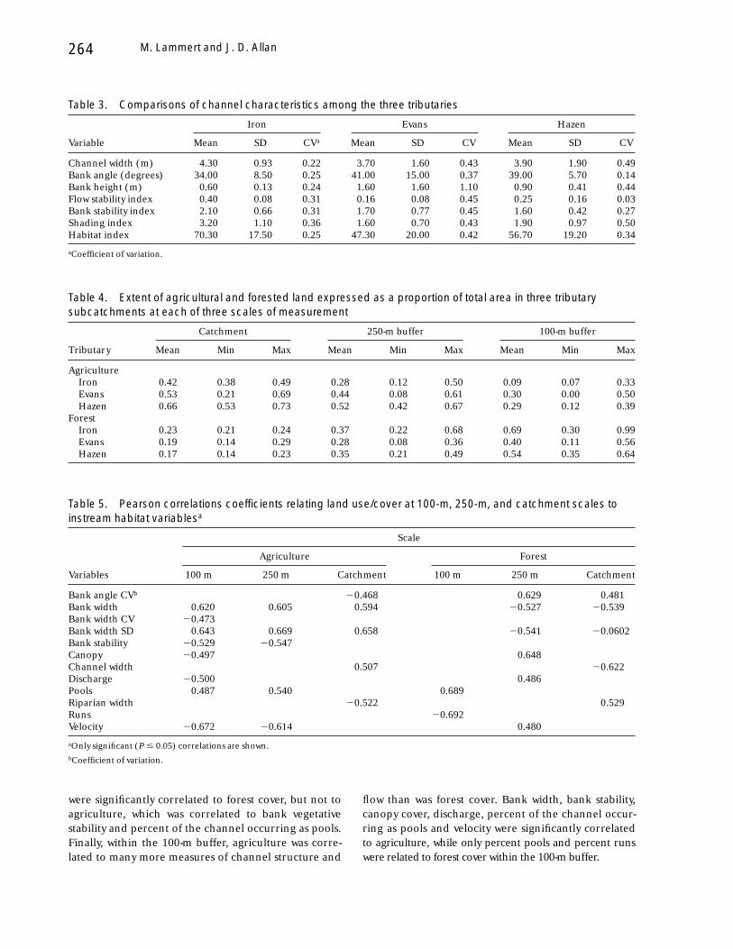
Although all study sites except the three downstreamsites on Hazen Creek are located on first-order reachesof the three tributaries, measures of channel morphol-ogy varied considerably among tributaries. Iron Creekhad the widest channels, as well as lowest bank heightsand bank angles. The flow stability index and ratio ofbankfull width to bankfull depth reflect this morphol-ogy and suggest that Iron Creek is less flashy than theother two tributaries. Iron Creek also had the moststable bank vegetation and highest shading (Table 3),

and the highest mean HI scores (mean 6 SD:70.33 6 17.53) followed by Hazen (56.67 6 19.19, thenEvans 47.33 6 19.95). However, mean HI scores werenot significantly different among tributaries (F 5 2.24,df 5 2, P 5 0.140). HI scores were most highly corre-lated to substrate size and embeddedness (r 5 0.944and 0.912). However, embeddedness explained little ofthe remaining variation in HI scores as it was highlycorrelated to substrate size (r 5 0.866). Bank vegetationcondition was the second most important factor forhabitat condition, and with substrate explained 95% ofthe variation in HI scores. The best model for the HIwas HI score 5 14.71 1 3.38 (substrate) 1 2.87 (bankvegetative stability) (R2 5 0.95, P 5 0.000).

Landscape Assessment

At each of the three scales of measurement, compari-son of the tributaries revealed that Iron Creek has theleast agricultural land and the greatest amount offorested land of the three subcatchments (Table 4).Hazen Creek has more agricultural land than Evans,except within the 100 m buffer, where values are similar.Within its entire catchment, Hazen Creek has the lowestpercentage of forest cover of the three tributaries.However, within the 250-m and 100-m buffers, HazenCreek has more forested land than Evans Creek, andalmost as much as Iron Creek (Table 4).

Land use/cover percentages within each scale ofmeasurement—across the entire catchment, and withinthe 250-m and the 100-m buffers—were highly corre-lated. For agriculture, forest, wetland, and urban landuse/cover, all Pearson correlations ranged from 0.53 to0.99. These correlations were expected given that eachland use/cover displaces another. However, land usepatterns within each scale category were not consis-tently correlated. Urban land use differed little whethermeasured within a buffer or across the entire subcatch-ment, showing that urban land use was consistent in itsdistribution relative to the three streams. In contrast,forest cover percentages differed greatly by scale ofmeasurement (Pearson r values ranged from 20.29 to0.33), showing that forest cover is not evenly distributedthroughout the three subcatchments.

Relationships between instream and landscape variables.A number of instream physical variables were signifi-

cantly correlated to land use/cover categories at eachscale of measurement (Table 5). At the catchment scale,five habitat variables—bank angle coefficient of varia-tion, bank width, bank width standard deviation, chan-nel width, and the riparian index—were correlated tothe extent of forest and agriculture. At the 250-m bufferscale, correlations among habitat features and land usewere more variable. Canopy openness and discharge

Table 2. Pearson correlation matrix ofmacroinvertebrate assemblage measuresa

TAXA TMAY H8 EPT B-IBI ICI

TMAY 0.670H8 0.799 0.769EPT 0.767 0.919 0.781B-IBI 0.618 0.791 0.681 0.822ICI 0.782 0.828 0.820 0.914 0.713BI 20.515 20.648 20.476 20.712 20.755 20.669

aMeasures include two multimetric indexes: the benthic index of bioticintegrity (B-IBI) and the invertebrate community index (ICI); foursingle-value measures: number of taxa (TAXA), number of mayfly taxa(TMAY), Shannon diversity (H8), and number of Ephemeroptera,Plecoptera, and Trichoptera taxa (EPT); and the pollution tolerancebiotic index (BI). All correlations are significant at P # 0.05.


were significantly correlated to forest cover, but not toagriculture, which was correlated to bank vegetativestability and percent of the channel occurring as pools.Finally, within the 100-m buffer, agriculture was corre-lated to many more measures of channel structure and

flow than was forest cover. Bank width, bank stability,canopy cover, discharge, percent of the channel occur-ring as pools and velocity were significantly correlatedto agriculture, while only percent pools and percent runswere related to forest cover within the 100-m buffer.

Table 3. Comparisons of channel characteristics among the three tributaries

Variable

Iron Evans Hazen

Mean SD CVa Mean SD CV Mean SD CV

Channel width (m) 4.30 0.93 0.22 3.70 1.60 0.43 3.90 1.90 0.49Bank angle (degrees) 34.00 8.50 0.25 41.00 15.00 0.37 39.00 5.70 0.14Bank height (m) 0.60 0.13 0.24 1.60 1.60 1.10 0.90 0.41 0.44Flow stability index 0.40 0.08 0.31 0.16 0.08 0.45 0.25 0.16 0.03Bank stability index 2.10 0.66 0.31 1.70 0.77 0.45 1.60 0.42 0.27Shading index 3.20 1.10 0.36 1.60 0.70 0.43 1.90 0.97 0.50Habitat index 70.30 17.50 0.25 47.30 20.00 0.42 56.70 19.20 0.34

aCoefficient of variation.

Table 4. Extent of agricultural and forested land expressed as a proportion of total area in three tributarysubcatchments at each of three scales of measurement

Tributary

Catchment 250-m buffer 100-m buffer

Mean Min Max Mean Min Max Mean Min Max

AgricultureIron 0.42 0.38 0.49 0.28 0.12 0.50 0.09 0.07 0.33Evans 0.53 0.21 0.69 0.44 0.08 0.61 0.30 0.00 0.50Hazen 0.66 0.53 0.73 0.52 0.42 0.67 0.29 0.12 0.39

ForestIron 0.23 0.21 0.24 0.37 0.22 0.68 0.69 0.30 0.99Evans 0.19 0.14 0.29 0.28 0.08 0.36 0.40 0.11 0.56Hazen 0.17 0.14 0.23 0.35 0.21 0.49 0.54 0.35 0.64

Table 5. Pearson correlations coefficients relating land use/cover at 100-m, 250-m, and catchment scales toinstream habitat variablesa

Variables

Scale

Agriculture Forest

100 m 250 m Catchment 100 m 250 m Catchment

Bank angle CVb 20.468 0.629 0.481Bank width 0.620 0.605 0.594 20.527 20.539Bank width CV 20.473Bank width SD 0.643 0.669 0.658 20.541 20.0602Bank stability 20.529 20.547Canopy 20.497 0.648Channel width 0.507 20.622Discharge 20.500 0.486Pools 0.487 0.540 0.689Riparian width 20.522 0.529Runs 20.692Velocity 20.672 20.614 0.480

aOnly significant (P # 0.05) correlations are shown.bCoefficient of variation.


Relationships Between Biotic and PhysicalVariables

Relationships among major indexes. We compared mac-roinvertebrate and habitat measures to determine ifthey ranked sites similarly in terms of overall quality.Spearman’s rank correlation allowed us to make pair-wise comparisons of the B-IBI, ICI, BI, and HI at eachsite. This test showed that with one exception, rankingof the sites by IBI (fish) scores had the least concor-dance with rankings by other indexes. The IBI ranking

of sites was most consistent with the B-IBI (Spearman’sr 5 0.59), but the remaining correlations were belowr 5 0.50 (Lammert 1995). This result lends credence tothe view that indexes based on macroinvertebrates andfishes give somewhat different indications of streamcondition.

Plots of index scores against each other provided asecond means of comparing site rankings (Figure 4).The strongest linear correlation occurred between thetwo multimetric macroinvertebrate indexes, B-IBI and

Figure 4. Comparisons among three biomonitoring indexes, the fish index of biotic integrity, (IBI), two macroinvertebrateindexes, the index of community integrity (ICI) and the benthic index of biotic integrity (B-IBI); and a habitat index (HI), usingsimple linear regression. Individual points are the six sampling sites located on three tributaries. All three biotic measures show asimilar relationship to habitat quality. Higher correlations indicate that the metrics being compared provide similar rankings ofsites. The strongest relationship is between the two macroinvertebrate indexes.


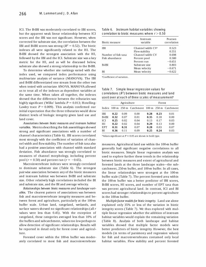
ICI. The B-IBI was moderately correlated to IBI scores,but the apparent weak linear relationship between ICIscores and the IBI was not significant. However, whencorrected for substrate size, the correlation between theIBI and B-IBI scores was strong (R2 5 0.52). The bioticindexes all were significantly related to the HI. TheB-IBI showed the strongest association with the HI,followed by the IBI and the ICI. Substrate size was a keymetric for the HI, and as will be discussed below,substrate also showed a strong relationship to the B-IBI.

To determine whether site rankings varied with theindex used, we compared index performance usingmultivariate analysis of variance (MANOVA). The IBIand B-IBI differentiated one stream from the other twowhen tested with univariate ANOVA. MANOVA allowedus to treat all of the indexes as dependent variables atthe same time. When taken all together, the indexesshowed that the difference between the tributaries washighly significant (Wilks’ lambda P 5 0.013; Hotelling-Lawley trace P 5 0.009). This analysis confirmed ourinitial expectation that the three tributaries would showdistinct levels of biologic integrity given land use andland cover.

Associations between biotic measures and instream habitatvariables. Metrics describing the fish assemblages showedstrong and significant associations with a number ofchannel characteristics (Table 6). IBI scores correlatedmost strongly with the coefficient of variation of chan-nel width and flow stability. The number of fish taxa alsohad a positive association with channel width standarddeviation. Fish abundance was strongly correlated tomeasures of channel morphology, including percentpool (r 5 0.50) and percent run (r 5 20.65).

Macroinvertebrate indexes were strongly correlatedto dominate substrate size (Table 6). The strongestpairwise association between any of the biotic measuresand instream habitat was between B-IBI and substratesize. Other relatively high correlations included the BIand substrate size, and the BI and average velocity.

Relationships between biotic measures and landscape vari-ables. The clearest pattern of associations was betweenfish and macroinvertebrate integrity measures and be-tween forest and agriculture, particularly at the 100-mbuffer scale. Urban land, rangeland, wetlands, andsurface waters showed no significant relationships (all rvalues were less than 0.45). With the exception ofrangeland, these categories averaged less than 10% ofthe buffers and subcatchment, values too low perhaps toallow detection of significant relationships. Results willbe reported in detail only for forest cover and agricul-ture.

Forested cover within the 100-m buffer was moder-ately correlated to most fish and macroinvertebrate

measures. Agricultural land use within the 100-m buffergenerally had significant negative correlations to allbiotic measures. Simple linear regression analysis wasused to explore further these trends in the relationshipbetween biotic measures and extent of agricultural andforested lands at the three landscape scales—the sub-catchment, 250-m buffer, and 100-m buffer. In all cases,the linear relationships were strongest at the 100-mbuffer scale (Table 7). The percent forested area withinthe 100-m buffer was a better predictor of IBI scores,B-IBI scores, HI scores, and number of EPT taxa thanwas percent agricultural land. In contrast, ICI and BIscores had stronger relationships to percent agriculturein the 100-m buffer.

Multiple factor models for biotic integrity. Land use aloneexplained only 35% or less of the variation in bioticintegrity scores (Table 7). We thus explored with mul-tiple linear regression whether the addition of instreamhabitat variables would explain the remaining variation(Table 8). Analysis of both landscape and habitatvariables showed that multiple factor models werebetter predictors of biotic integrity. However, the bestmodels (in terms of parsimony and regression values)for fish and macroinvertebrates contained only localhabitat variables. Flow stability and percent forested

Table 6. Instream habitat variables showingcorrelation to biotic measures where r . 0.50

Biotic measureInstreamvariable

Pearsoncorrelation

IBI Channel width CVa 0.523Flow stability 0.551

Number of fish taxa Channel width CV 0.698Fish abundance Percent pool 0.580

Percent run 20.651B-IBI Substrate size 0.803

Mean velocity 20.671BI Mean velocity 20.622

aCoefficient of variation.

Table 7. Simple linear regression values forcorrelations (R2) between biotic measures and landuse/cover at each of three scales of measurementa

Index

Agriculture Forest

100 m 250 m Catchment 100 m 250 m Catchment

IBI 0.22 0.09 0.00 0.28 0.23 0.01B-IBI 0.32 0.07 0.01 0.35 0.18 0.00ICI 0.25 0.02 0.04 0.13 0.17 0.03HI 0.22 0.02 0.04 0.29 0.13 0.00EPT 0.31 0.31 0.07 0.28 0.03 0.07BI 0.36 0.11 0.09 0.25 0.24 0.03

aValues significant at P # 0.05 are shown in bold type.


land in the 100-m buffer together explained 44% of thevariation in IBI scores. A model with flow stability andthe standard deviation of channel width proved aslightly better predictor of IBI scores (R2 5 0.47), indi-cating that at-site channel features predicted the IBI atleast as well as land use measures.

Substrate size explained the greatest proportion ofthe variance in all of the multimetric macroinvertebrateindexes. For the B-IBI, flow stability was a significantadditional factor, increasing the variance explained by20% (R2 5 0.814). Flow stability was also the nextstrongest variable after substrate size in explainingvariation in the ICI, increasing the R2 by 10%(R2 5 0.42). Finally, substrate size explained 45% of thevariance in BI scores alone. The addition of averagevelocity to the model increased the variance explainedby 32% (R2 5 0.78).

Discussion

We demonstrated that habitat and immediate landuse predicted biotic integrity in three warmwater streamsin the midwestern United States. Flow stability for fishand dominant substrate for macroinvertebrates weregood predictors of biotic condition. Our results alsodemonstrate that land use within 100-m of the stream

was significantly related to biotic integrity. Catchment-wide (regional) land use showed no relationship. Theseresults do not, however, provide a conclusive answer tothe general question raised by landscape ecologistsHunsaker and Levine (1995) of whether local or catch-ment-wide factors have more of an impact on thebiologic integrity of streams. Based on this and aprevious study previous of the River Raisin watershed(Roth and others 1996), we recommend that thisquestion not be cast as ‘‘either—or.’’ The physicalfactors we measured have effects and are the result ofprocesses that occur at multiple scales. We believe thatour study demonstrates that the ability to tease apartsources of variation turns greatly on sampling design.

The finding that local land use and habitat werebetter predictors of biotic integrity than regional landuse contrasts with findings of a previous study of theRiver Raisin watershed that found regional land astronger predictor of fish assemblages than local habi-tat. Roth and others (1996) sampled broad areas of theRaisin River basin, and their data represent regionalconditions for at least seven subcatchments. In thepresent design, sites were located close together andregional land use did not differ greatly within eachsubcatchment. Our 18 sites, in fact, represented onlythree regional conditions. As Poff and Allan (1995)note, the ability to detect a significant relationshipdepends on the range of conditions within the variablegroup of interest. Therefore, the scale of measurementin the present study was most appropriate for determin-ing the effects of local variation, which was our intent.

Local habitat variables were shown to be superior toland use in predicting biotic integrity, particularly formacroinvertebrates. Predictive models between landuse and biotic integrity were greatly enhanced by theaddition of instream variables (see Table 8). Channelmorphology and substrate conditions (for macroinverte-brate only) actually explained more of the variation infish and macroinvertebrate biotic integrity than didland use/cover alone. In several cases, land use ex-plained no additional variance beyond that explainedby substrate and flow stability. These results suggest thatriparian land use and instream habitat are not indepen-dent variables in this stream system, supporting thehypothesis of Frissell and others (1986) that the re-gional configuration of a watershed constrains the localstructure. Richards and others (1996) found that localstream habitat could be traced to catchment-wide im-pacts as well as local land use and inherent characteris-tics of the land immediately adjacent to the stream.However, they also concluded that we are limited in ourability to measure these effects by data resolution and

Table 8. Multiple linear regression models to predictbiotic measuresa

Dependent variable Independent variable R2 DR2

IBI 1 Percent forested,100 m buffer

0.276

With land useincluded

2 Flow stability 0.435 10.159

3 Channel width SD 0.525 10.090Without land use

included1 Flow stability 0.303

2 Channel width SD 0.468 10.165B-IBI 1 Substrate size 0.645

2 Flow stability CVb 0.814 10.1693 Percent forested,

100 m buffer0.872 10.058

4 Percent run 0.889 10.0175 Bank height 0.895 10.007

ICI 1 Substrate size 0.2972 Flow stability 0.423 10.1263 Sinuosity 0.480 10.057

BI 1 Substrate size 0.4502 Velocity 0.777 10.3273 Percent agriculture,

100 m buffer0.795 10.018

aThe single best predictor variable is listed first as the independentvariable. The next best predictors are evaluated for their reduction ofresidual variation (R2 and DR2).bCoefficient of variation.


confounding factors such as geology and land usepractices.

We expected the biological condition of the threetributaries to be more distinct based on differences inagricultural land use in each subcatchment, initialreconnaissance, and the conclusions of Roth and others(1996) regarding the importance of regional land use.However, along each stream, sampling sites variedgreatly in channel structure and forest cover, and wethus found that variation in the faunal assemblageswithin tributaries was greater than that between tributar-ies. Multiple lines of evidence showed that sites on IronCreek had the greatest ecological integrity. However,the average biotic and habitat condition of Iron Creekand Hazen Creek were not distinguishable, althoughHazen Creek had the highest agricultural land use forall three scales considered. The two creeks were similarin forest cover within the 100-m buffer (Table 4), andchannelization was evident in Evans Creek, demonstrat-ing the importance of local habitat alteration. Thesefindings recommend further investigation of the effectof the longitudinal forest configuration on streams.

Difference in habitat, possibly unrelated to land use,also might contribute to differences among tributariesin their biotic indexes (Schlosser 1987). Higher abun-dances of fish at the Hazen Creek sites than at the IronCreek sites suggest that greater pool volume in HazenCreek compensated for apparently superior habitatconditions in Iron Creek. While Iron Creek had greaterflow stability and exhibited habitat features that sug-gested a less degraded stream (Table 2), Hazen Creek’schannel was 22% pool, compared to only 9% of Iron’schannel, which provided habitat to support greaterconcentrations of fish. Iron Creek did have higher IBIscores due to higher species diversity and more individu-als of intolerant species, but high abundances of fish atHazen Creek made their biotic condition hard todistinguish with the IBI (Figure 3).

The sensitivity, validity, and calibration of the bioticmeasures also influenced the ability to discern differ-ences among sites and tributaries. Use of the IBI iswidespread across the Midwest and has been employedin at least two studies of the River Raisin watershed(Fausch and others 1984; Roth and others 1996). Thisuse assured availability of reference data at least at theecoregional scale. No such reference data were avail-able for the B-IBI. Thus, we used that index to rank sitesrelative to each to other. Further validation studies ofthe type described in Kerans and Karr (1994), and Karrand Chu (1997) will be required to establish the B-IBI asa means to detect water quality impacts in this region.

We chose to use a multiplicity of indexes to search forconsistent relationships between biologic condition,

land use, and instream habitat. High correlations be-tween single-factor and multiple-factor indexes suggestthat the indexes employed in this study were equallyuseful for determining the relative condition of studylocations. For the B-IBI and ICI, taxonomic diversitymetrics explained most of the variance in scores. Thisfinding supports the view of Resh (1994) that simpleindexes can be as effective as indexes that requireadditional analysis to assign taxa to functional groups.

IBI scores were more strongly correlated to landuse/cover than were macroinvertebrate indexes, whichwere very strongly correlated to local habitat measures.These findings support the conclusion of Plafkin andothers (1989) that macroinvertebrate assemblages aremore indicative of local habitat conditions. While habi-tat heterogeneity creates refugia for fish and macroinver-tebrates (Scarnecchia 1988, Sedell and others 1990),fish assemblages did not show as strong relationship tomeasures of habitat structure in comparison to macroin-vertebrates. Substrate size, which is positively associatedwith substrate heterogeneity (Minshall 1984), wasstrongly correlated to most macroinvertebrate assem-blage measures.

The nonconcordance of fish and macroinvertebratebiotic integrity may indicate that habitat measurementsdid not reflect variability in stream structure at a scalemeaningful to fish. The mobility of fish and theirpossible linkage into larger metapopulations may re-duce their sensitivity to the patchiness of stream habitat(Schlosser and Angermeier 1995). Angermeier (1987)found that regionally abundant fish species are lesssensitive to habitat differences across space and time.The fish assemblages in this study were dominated by afew common taxa, which may explain why the fish didnot have as well-defined associations with habitat asmacroinvertebrates.

The successive studies of the River Raisin watershed(Roth and other 1996, Lammert 1995) offer significantinsight into the effect of spatial scale on detecting landuse influence on stream biotic integrity. The unex-plained variation in biotic condition does, however,warrant further study. Richards and other (1996, 1997)and Wiley and others (1997) suggest that mappingsources of variation in aquatic assemblages requires aspatially hierarchical sampling design. Wiley and others(1997) also demonstrate the need to account for tempo-ral variation. We recognize that nested designs repli-cated in space and time are ideal to develop thecomprehensive picture of local and regional streamecosystem mechanisms described by Wiley and others(1997), but we believe that our study shows that singleevent sampling is an effective and economic means to


uncover patterns and hone hypotheses for future inves-tigations.

Acknowledgments

Funding for this study was provided by the USDepartment of Agriculture under the McIntire-StennisCooperative Forestry Research Act (P.L. 87-778) and aUSDA-CRSEES award. Land use/cover data were pro-vided by the Michigan Department of Natural Re-sources under a cooperative agreement. We thank JohnFay for GIS assistance and production of the mapfigures, Gary Fowler for advice on statistical analysis,and Mike Wiley for his input throughout this project.We thank Robin Abell, Andrew Lillie, Kate Bucking-ham, Dan Johnson, and many others for their assistancein gathering data, and Suzanne Sessine for assistance inprocessing macroinvertebrate samples. Finally, thanksare due to James Karr and Chris Frissell for providingdetailed and thoughtful reviews of the manuscript.

Literature Cited

Addicott, J. F., J. M. Aho, M. F. Antolin, D. K. Padilla, J. S.Richardson, and D. A. Soluk. 1987. Ecological neighbor-hoods: Scaling environmental patterns. Oikos 49:340–346.

Allan, J. D. 1995. Stream ecology: structure and function ofrunning waters. Chapman and Hall, London.

Angermeier, P. L. 1987. Spatiotemporal variation in habitatselection by fishes in small Illinois streams. Pages 52–60 inW. J. Matthews and D. C. Heins (eds.), Community andevolutionary ecology of North American stream fishes.University of Oklahoma Press, Norman, Oklahoma.

Cummins, K. W. 1988. The study of stream ecosystems: afunctional view. Pages 247–262 in L. R. Pomeroy and J. J.Alberts (eds.), Concepts of ecosystem ecology: a compara-tive view. Springer-Verlag, New York.

Downes, B. J., P. S. Lake, and E. S. G. Schreiber. 1993. Spatialvariation in the distribution of stream invertebrates: Implica-tions of patchiness for models of community organization.Freshwater Biology 30:119–132.

Enslin, W. 1991. C-MAP. Center for Remote Sensing, MichiganState University, East Lansing, Michigan.

Environmental Systems Research Institute. 1994. PC ARC/INFO.

Fausch, K. D., J. R. Karr, and P. R. Yant. 1984. Regionalapplication of an index of biotic integrity based on streamfish communities. Transactions of the American Fisheries Society113:39–55.

Fay, J. P. 1995. Using GIS to model nonpoint source pollutionin an agricultural watershed in southeast Michigan. Unpub-lished master’s thesis. School of Natural Resources andEnvironment, University of Michigan, Ann Arbor, Michigan.

Frissell, C. A., W. J. Liss, C. E. Warren, and M. D. Hurley. 1986.A hierarchical framework for stream habitat classification:

Viewing streams in a watershed context. EnvironmentalManagement 10(2):199–214.

Gordon, N. D., T. A. McMahon, and B. L. Finlayson. 1992.Stream hydrology: An introduction for ecologists. JohnWiley & Sons, Chichester, England.

Gorman, O. T., and J. R. Karr. 1978. Habitat structure and fishcommunities. Ecology 59:507–515.

Hawkins, C. P., J. L. Kershner, P. A. Bisson, M. D. Bryant, L. M.Decker, S. V. Gregory, D. A. McCullough, C. K. Overton, G.H. Reeves, R. J. Steedman, and M. K. Young. 1993. Ahierarchical approach to classifying stream habitat features.Fisheries 18(6):3–10.

Hilsenhoff, W. L. 1987. An improved biotic index of organicstream pollution. Great Lakes Entomologist 20:31–39.

Hilsenhoff, W. L. 1988. Rapid field assessment of organicpollution with a family-level biotic index. Journal of the NorthAmerican Benthological Society 7(1):65–68.

Hunsaker, C. T., and D. A. Levine. 1995. Hierarchical ap-proaches to the study of water quality in rivers. BioScience45(3):193–203.

Karr, J. R., and E. W. Chu. 1997. Biological monitoring andassessment: using multimetric indexes effectively. EPA 235-R97-001. US Environmental Protection Agency, Washing-ton, DC.

Karr, J. R., K. D. Fausch, P. L. Angermeier, P. R. Yant, and I. J.Schlosser. 1986. Addressing biological integrity in runningwaters: A method and its rationale. Special Publication 5.Illinois Natural History Survey, Champaign, Illinois.

Kerans, B. L., and J. R. Karr. 1994. Development and testing ofa benthic index of biotic integrity (B-IBI) for rivers of theTennessee Valley Authority. Ecological Applications 4(4):786–785.

Lammert, M. 1995. Assessing land use and habitat effects onfish and macroinvertebrate assemblages: Stream biotic integ-rity in an agricultural watershed. Unpublished master’sthesis. School of Natural Resources and Environment,University of Michigan, Ann Arbor, Michigan.

Lenat, D. R. 1993. A biotic index for the southeastern UnitedStates: derivation and list of tolerance values, with criteriafor assigning water-quality ratings. Journal of the North Ameri-can Benthological Society 12(3):279–290.

Malmqvist, B., and M. Maki. 1994. Benthic macroinvertebrateassemblages in north Swedish streams: environmental rela-tionships. Ecography 17:9–16.

Meador, M. R., S. R. Hupp, T. F. Cuffney, and M. E. Gurtz.1993. Methods for characterizing stream habitat as part ofthe National Water-Quality Assessment Program. US Geologi-cal Survey, Open-File Report 93–408.

MDNR (Michigan Department of Natural Resources). 1989.Qualitative biological and habitat survey protocols for wad-able streams and rivers. GLEAS procedure No. 51. MichiganDepartment of Natural Resources, Surface Water QualityDivision, Great Lakes Environmental Assessment Section.

Mid-Atlantic Coastal Streams Workgroup. 1993. Standard oper-ating procedures and technical basis: macroinvertebratecollection and habitat assessment for low gradient, non-tidalstreams. US Environmental Protection Agency, Region III,Wheeling, West Virginia, 48 pp. (draft).


Minshall, G. W. 1984. Aquatic insect-substratum relationships.Pages 358–400 in V. H. Resh and D. M. Rosenberg (eds.),The ecology of aquatic insects. Prager, New York.

Ohio EPA. 1989. Biological criteria for the protection ofaquatic life: Volume III. Standardized biological field sam-pling and laboratory methods for assessing fish and macro-invertebrate communities. Division of Water Quality Moni-toring and Assessment, Columbus, Ohio.

Osborne, L. L., and D. A. Kovacic. 1993. Riparian vegetatedbuffer strips in water-quality restoration and stream manage-ment. Freshwater Biology 29:243–258.

Osborne, L. L., and M. J. Wiley. 1992. Influence of tributaryspatial position on the structure of warmwater fish commu-nities. Canadian Journal of Fisheries and Aquatic Science 49(4):671–681.

Osborne, L. L., B. Dickson, M. Ebbers, R. Ford, J. Lyons, D.Kline, E. Rankin, D. Ross, R. Sauer, P. Seelbach, C. Speas, T.Stefanavage, J. Waite, and S. Walker. 1991. Stream habitatassessment programs in the states of the AFS North CentralDivision. Fisheries 16(3):28–35.

Plafkin, J. L., M. T. Barbour, K. D. Porter, S. K. Gross, and R. M.Hughes. 1989. Rapid bioassessment protocols for use instream and rivers: benthic macroinvertebrates and fish.EPA/444/4-89-011. US Environmental Protection Agency,Washington, DC, 150 pp.

Poff, N. L., and J. D. Allan. 1995. Functional organization ofstream fish assemblages in relation to hydrological variabil-ity. Ecology 76(2):606–627.

Quinn, J. M., and C. W. Hickey. 1990. Characterization andclassification of benthic invertebrate communities in 88New Zealand rivers in relation to environmental factors. NewZealand Journal of Marine and Freshwater Research 24:387–409.

Resh, V. H. 1994. Variability, accuracy, and taxonomic costs ofrapid assessment approaches in benthic macroinvertebratebiomonitoring. Bollettino di Zoologia 61:375–383.

Resh, V. H., and J. K. Jackson. 1993. Rapid assessmentapproaches to biomonitoring using benthic macroinverte-brates. Pages 195–233 in V. H. Rosenberg and D. L. Resh(eds.), Freshwater biomonitoring and benthic inverte-brates. Chapman and Hall, New York.

Richards, C., and G. E. Host. 1994. Examining land useinfluences on stream habitats: A GIS approach. WaterResources Bulletin 30(4):729–738.

Richards, C., G. E. Host, and J. W. Arthur. 1993. Identificationof predominant environmental factors structuring streammacroinvertebrate communities within a large agriculturalcatchment. Freshwater Biology 29:285–294.

Richards, C., L. B. Johnson, and G. E. Host. 1996. Landscape-scale influences on stream habitats and biota. CanadianJournal of Fisheries and Aquatic Science 53(suppl. I):295–311.

Richards, C., R. J. Haro, L. B. Johnson, and G. E. Host. 1997.Catchment and reach-scale properties as indicators of mac-roinvertebrate species traits. Freshwater Biology 37:219–230.

Rosenberg, D. M., and V. H. Resh (eds.). 1993. Freshwaterbiomonitoring and benthic macroinvertebrates. Chapmanand Hall, New York.

Rosgen, D. L. 1994. A classification of natural rivers. Catena22:169–199.

Roth, N. E., J. D. Allan, and D. E. Erickson. 1996. Landscapeinfluences on stream biotic integrity assessed at multiplespatial scales. Landscape Ecology 11(3):141–156.

Scarnecchia, D. L. 1988. The importance of streamlining ininfluencing fish community structure in channelized andunchannelized reaches of a prairie stream. Regulated Rivers,Research and Management 2:155–166.

Schlosser, I. J. 1982. Fish community structure and functionalong two habitat gradients in a headwater stream. EcologicalMonographs 52:395–414.

Schlosser, I. J. 1985. Flow regime, juvenile abundance and theassemblage structure of stream fishes. Ecology 66:1484–1490.

Schlosser, I. J. 1987. A conceptual framework for fish commu-nities in small warmwater streams. Pages 17–24 in W. J.Matthews and D. C. Heins (eds.), Community and evolution-ary ecology of North American stream fishes. University ofOklahoma Press, Norman, Oklahoma.

Schlosser, I. J. 1991. Stream fish ecology: A landscape perspec-tive. BioScience 41(10):704–712.

Schlosser, I. J., and P. L. Angermeier. 1995. Spatial variation indemographic processes of lotic fishes: conceptual models,empirical evidence, and implications for conservation. Ameri-can Fisheries Society Symposium 17:392–401.

Sedell, J. R., G. H. Reeves, F. R. Hauer, J. A. Stanford, and C. P.Hawkins. 1990. Role of refugia in recovery from distur-bances: modern fragmented and disconnected river sys-tems. Environmental Management 14(5):711–724.

Shannon, C. E. 1948. A mathematical theory of communica-tion. Bell Systems Technical Journal 27:379–423, 623–656.

Steedman, R. J. 1988. Modification and assessment of an indexof biotic integrity to quantify stream quality in southernOntario. Canadian Journal of Fisheries and Aquatic Science45:492–501.

Taylor, C. M., M. R. Winston, and W. J. Matthews. 1993. Fishspecies-environment and abundance relationships in a GreatPlains river system. Ecography 16:16–23.

Townsend, C. R., and A. G. Hildrew. 1994. Species traits inrelation to a habitat templet for river systems. FreshwaterBiology 31(3):265–275.

Wiens, J. A. 1989. Spatial scaling in ecology. Functional Ecology3:385–397.

Wiley, M. J., L. L. Osborne, and R. W. Larimore. 1990.Longitudinal structure of an agricultural prairie system andits relationship to current ecosystem theory. Canadian Jour-nal of Fisheries and Aquatic Science 47(2):373–384.

Wiley, M. J., S. L. Kohler, and P. W. Seelbach. 1997. Reconcilinglandscape and local views of aquatic communities: Lessonsfrom Michigan trout streams. Freshwater Biology 37:13–148.


environmental auditing assessing biotic integrity …dallan/pdfs/lammert_allan.pdf · relate...

Documents