December 1990 LIDS-P-2010

Envelope Detection of Orthogonal Signalswith Phase Noise 1

Murat Azizoglu and Pierre A. Humblet

Laboratory for Information and Decision Systems

Massachusetts Institute of Technology

December 12, 1-990

Abstract

We analyze the performance of receivers which use envelope detection at IF to

detect optical signals with orthogonal modulation formats. We obtain exact closed-

form expressions for the error probability conditioned on the normalized envelope.

The only information necessary for obtaining the unconditional error probability isthe set of tilted moments of the envelope. We then provide an approximation to this

envelope which is not only accurate to the first order in phase noise strength, but

also has the same range as the actual random envelope. We use this approximation

to obtain the bit error performance of the three receiver models that we consider.

We also provide a tight lower bound in closed-form. Finally we extend the analy-

sis to N-ary FSK to observe the improvement due to increased bandwidth use and

transmitter/receiver complexity.

1This research was supported by NSF under grant NSF/8802991-NCR and by DARPA under

grant F19628-90-C-0002

1 Introduction

Coherent optical communication systems provide an efficient way of sharing the huge

bandwidth of single mode optical fiber among different users of the future high-speed

networks. The two important reasons for this efficiency are the improved receiver

sensitivity and increased channel density over direct detection systems. As a result,

considerable effort has gone into developing coherent systems and into characterizing

and overcoming problems to allow coherent technology to become a practical alter-

native to direct detection optical systems. Among major problems associated with

coherent technology is the fact that the phase of the light emitted from a semicon-

ductor laser exhibits random fluctuations due to spontaneous emissions in the laser

cavity [1]. This phenomenon is commonly referred to as "phase noise". Phase noise

has two important effects on the performance of optical networks. The first of these

effects is the broadening of the spectrum emitted by the users of the network, which

causes interchannel interference and thus necessitates wider channel spacing. This is

especially dominant at low data rates where channels occupy small bandwidth. The

second effect is the incomplete knowledge and the time-varying nature of the phase

which makes the correct retrieval of the transmitted data bits more difficult for the

receiver. While the first effect results in inefficient use of the available bandwidth,the second one causes a degradation of the bit error rate of the transmitter/receiver

pairs.

It is the second effect above that we consider in this paper. This problem has

received much attention in the recent years. Various performance analyses for different

modulation formats and receiver structures exist in the literature [2, 3, 4, 5, 6, 7].

However, since researchers use different sets of assumptions and approximations in

their work, it is difficult to reconcile their results and to agree on the quantitative

effect of phase noise on coherent systems. The difficulty seems to arise from the fact

that the Brownian motion model of the phase noise, which is well-tested and agreed

upon, results in a random process that is both nonlinear and nonstationary. Thus,

as one moves through different stages of a nontrivial receiver, the exact statistical

characterization of the randomness due to phase noise becomes increasingly difficult.

One needs to invoke a sequence of assumptions and approximations to overcomethese difficulties. Naturally, the confidence that the real systems will operate within

a reasonable margin of the predictions of the analyses depends on the number and

the nature of these assumptions and approximations.

It is reasonable to expect that the modulation formats which are the least to suf-

fer from phase noise will be those with asymmetric constellations in the signal space,

e.g. on-off-keying (OOK) and frequency-shift-keying (FSK). These two modulation

formats were considered recently by Foschini and his colleagues in [3]. They formu-

lated and treated the problem with a minimal number of approximations. Their work

provides a rigorous framework upon which the researchers in the field may agree and

improve on. As a result, a considerable number of papers have resulted from their

model in a relatively short time [7, 8, 4]. The work reported here also conforms to the

receiver model of [3]. We consider orthogonal modulation formats in this paper, e.g.

FSK and orthogonal polarization modulation. However the results can be general-

ized to obtain the performance of OOK as well. We describe the receiver models and

the problem in next section. We obtain closed-form expressions for the probability

of error conditional on the squared envelope of a normalized phase noisy signal, for

different receiver forms. We provide an approximation which is close to the actual

envelope and whose moments are readily available. We compute the probability den-

sity function of this approximate envelope from its moments using a method based on

Legendre polynomials. We then use this density function to remove the conditioning

on the error probability and, thus, to obtain the error performance of the systems

under consideration. We also provide a lower bound to the error probability of the

double-filter receiver which is very close to the actual error probability. Therefore this

lower bound, which is very easy to compute, can be used to estimate the performance.

Finally, we extend the analysis to the case of N-ary FSK where we provide very

tight upper and lower bounds to the bit error probability.

2 Problem Description

The received optical signal is first processed by an optical heterodyne receiver shown

in Figure 1 for FSK signals. Polarization modulation would require a polarization

beam splitter and a pair of photodetectors. Optical heterodyning transforms the

signal from optical frequency to intermediate frequency. The IF signal output r(t) is

to be further processed by the IF receiver. This IF processing is the main focus of

this paper.

The IF receiver structure that we consider in this paper is shown in Figure 2 where

the incoming signal is corrupted by phase noise and additive noise. The front end

of this receiver is the standard quadrature receiver that performs envelope detection

2

of FSK signals. The correlators and integrators perform a bandpass filtering to limit

the noise power corrupting the signal. Since the integrators integrate their inputs

over a duration T' the effective bandwidth of the filter is 1/T'. For a uniformly

distributed phase uncertainty which is constant over the bit duration the optimum

value of T' is the bit duration T. However, when the signal is corrupted by phase

noise, the spectrum of the signal is broadened. Therefore a wider filter bandwidth,

equivalently smaller integration times, may be necessary. For analytical convenience,

we only consider the case where the ratio T/T' is a positive integer M as in [3].

The outputs of the in-phase and quadrature branch integrators in Figure 2 are

squared and then added to perform the envelope detection. The remaining processing

depends on the value of M.. For M = 1, the adder outputs are sampled at the end

of the bit duration and the two values are compared to reach a decision about the

transmitted data bit. We call the receiver with M = 1 a single sample receiver since

only one sample is taken during a bit duration. For AM > 2, the adder outputs are

sampled every T' seconds resulting in M samples per bit. The way these samples

are processed depends on the complexity that one desires. One simple strategy is to

discard all but the last one of these samples and to use the last sample as in the single

sample receiver. A more efficient way is to average these M samples and compare the

two averages. This averaging is not the optimlalprocessing of the samples. However

since it can be performed by a lowpass filter it is a practical reception strategy to

implement.

We classify the reception strategies above into three categories. The first is the

single sample receiver, the second one is the multisample receiver with single fil-

tering and the third one is the mIultisample receiver with double filtering. These

receiver structures were first suggested by Kazovsky et. al. in [10] for ASK mul-

tiport homodyne receivers. In the framework of [10], the single sample receiver isthe conventional matched-filter receiver, the single-filter receiver is the conventional

receiver with a widened filter, and the double filter receiver is the wide-band filter-rectifier-narrowband filter (WIRNA) structure. It was also noticed in [10] that if the

M samples of the double filter receiver are viewed as coming from M distinct chan-

nels (or from a fast frequency-hopped spread spectrum system), then the receiver is

functionally equivalent to the noncoherent receiver for multichannel signaling treated

in [11]. Some of our results, in particular the conditional error probability given by

Equation (19), may be obtained by using the results of [11]. However, we will proceed

independently for the sake of completeness.

3

2.1 Single Sample Receiver

We first consider the single sample receiver. This receiver is the optimal receiver when

the phase of the received signal has uniform distribution and is time-invariant. Theerror probability for this case has a simple closed-form (1/2 e-Eb/2N) [12]. We willsee that a similar (but more complicated) result can be obtained in the phase noisycase.

We assume that the received IF signal is the FSK signal corrupted by additivenoise and phase noise:

r(t) = Acos(2'rfit + 0(t)) + n(t) i = 0,1 (1)

where fo and fi are the frequencies for "0O" and "1" respectively. The phase noise9(t) is a Brownian motion process described by

0(t) = 2rjt jl(T)d- (2)

with ,U(r) being a zero-mean white Gaussian process with two-sided spectral density

13/27r. Then 0(t) is a zero-mean Gaussian process with zero-mean and variance 2i7r/t;

/3 is the combined linewidth of the source and local oscillator lasers. The additive

noise n(t) in (1) is a white Gaussian process with two-sided spectral density No/2. Weassume that the difference between fi and fo is much larger than the filter bandwidth

1/T', so that when a "0O" is transmitted, the integrator outputs of the lower branch

integrators in Figure 2a contain no signal component, and vice versa. With this

assumption, when a "0O" is transmitted the sampler outputs at time T can be written

as

YO = | A Ae (t ) dt + nco + jn.o|

Y1 = inci + jns l2 (3)

where nci and n,i are statistically independent and identically distributed (i.i.d.)

Gaussian random variables with zero-mean and variance o2 = NoT/4. Due to sym-

metry, the error probability is given by

P, = Pr(Yo < I) Y (4)

We will now condition the error probability on the amplitude of the phase noise

integral in (3). We define

4T4 ei(t)dt (5)

Then the conditional density of Y} can be easily found as2

p(yolY) = I2 --( °+Y2)/22 (Y / ) (6)

while Y1 has an exponential density given by

1 (7)p(yl) = 2 e-/2 . (7)

Therefore the conditional error probability comes as a result of the classical problem

of incoherent detection of orthogonal signals as [12]

Pe(Y) = -e-Y2/22 (8)2

Let's now express Y in a different form. From (5), we have

y AT eJ(TU) du

Since O(Tu) has variance 27r/Tu, Y can be written in terms of standard Brownian

motion +(t) (i.e. that with variance t) as

ATY = 2 || eji(t) dt

where ay 2i7roT. Now if we define the random variable X(-) as

2

X(Y) fo

(8) can be written in terms of X as

Pe(X) = le- x(')/2 (10)

where ~ = A 2T/2No is the signal-to-noise ratio. Therefore Pe is given by

P = Ex [e - d x(' ) / 2] (11)

In the case with no phase noise ('y = 0), this reduces to 1/2e-4 /2 as it should.

An immediate implication of (11) is that there does not exist a bit-error-rate-

floor, i.e. a nonzero error probability that exists even when ~ tends to o0, for the

2 For notational convenience we indirectly address the random variable that a density function

refers to with its argument, i.e., p(y) stands for py(y) in the more standard notation.

5

single sample receiver, provided that the probability density function of X('y) does

not contain a delta function at the origin 3

To determine P, from (11) we have to obtain either the probability density function

or the moment generating function of X. Therefore the random variable X plays a

key role in the performance analysis of the single sample receiver. In the next section,

we will show that this is also true for the multisample receivers that we consider.

2.2 Multisample Receivers

In the previous section, we mentioned that the receiver may use a shorter integration

time T' than the full bit duration T. The advantage of this scheme is that the phase

is not allowed to wander too much so that the amount of collected signal energy may

not drop below undesirable levels. Equivalently, the bandwidth of the IF filter is

increased to pass more of the signal power. If only the last of the M samples, the

one at t = T, is used, then the received signal is effectively processed only during

the interval (T- T',T), hence there is a drop in the received signal-to-noise ratio

by a factor of 1/M. However, since the phase is allowed to change in an interval

of length T', the effective value of -y also drops by a factor of 1/M. (This can be

observed by repeating the calculations of the previous section when T is replaced by

T'.) Therefore the probability of error for the multisample receiver with single filter

is given by

Pe = Ex [2.e X( )/2M] . (12)

An inspection of (12) shows that when the signal-to-noise ratio and/or the phase

noise strength is small, the optimal value of M will be small. However, for large

signal-to-noise ratios and large phase noise values, it may be worthwhile to sacrifice

from the signal energy while alleviating the effect of phase noise.

The single-filter receiver uses only one of the M available samples. Thus the

single-filter receiver is, in fact, a single sample receiver with widened front end filter

bandwidth. The efficiency of this receiver would be improved if all the M samples

were used in the decision process. A simple processing of these samples is averaging,

which may be accomplished by low-pass-filtering the sum of the outputs of the square-

law devices [3]. The result is the multisample double-filter receiver that we analyze

below. Note that this receiver is not the (still unknown) receiver which minimizes the

3Note that the inherent error floor in FSK due to the finite frequency separation [13, 5] is neglectedin our model.

6

probability of error. It is closely related to the optimal receiver for the case wherethe phase noise process O(t) is piecewise constant and takes M independent uniformly

distributed values during a bit interval. In this case, the optimal receiver averagesthe square root of the samples when the signal-to-noise ratio is high.

In the case of a "O" being transmitted, the lowpass filter outputs will be

M

Yo = E Ix(k) + no(k) + jno(k)l (13)k=l

M

Y, = E in,,(k) + jni(r k)l2 (14)k=l

where x(k) is given byA r kT'

x(k) = - eje (t) dt2 J(k-1)T'

and all the additive noise samples are i.i.d. zero-mean Gaussian with variance

a2 = NoT'/4 .

Since O(t) has independent increments, x(k) are statistically independent. Further-more, since O(t) has stationary increments, Ix(k)l will be identically distributed4 .Then each of the terms in (13) and (14) obey the distributions in (6) and (7) respec-tively. (Y in (6) is replaced by Ix(k)l.) In particular, since each term in (14) has

i.i.d. exponential distribution, Y, has a Gamma distribution with parameters M and

1/2a2 . It is convenient to normalize YO and Y1 via

Vi= 2 i = 0,1.2a2

Then V1 has the density function

M-1

p(vl) = (M -)!- v > o . (15)

Due to symmetry, the probability of error is given by

Pe = Pr(Vo < V)

- k=o k-e Op(v o) dvo (16)k=0

4This also implies that the envelopes preserve their statistical properties from one bit to another.So we can consider the first bit in the performance analysis without loss of generality.

7

where p(vo) is the density function of Vo. This density appears to be difficult to obtainin closed-form. Therefore, we will first condition (16) on the phase noisy envelopes.

Given {x(k): 1 < k < M}, Vo is the sum of squares of 2M independent Gaussianrandom variables, the density of which is given by [12]

p(vol{x(k)}) = (1) e-(Vo+r)IM_1 ( 4rvo) Vo > 0 (17)

where IM-1(') is the modified Bessel function of order M - 1 and r is defined as

1 Mr = E X( k) 22a 2 k=

Note that the conditional density of Vo depends on {x(k)} only through the sum of

their squared amplitudes. This enables us to proceed further and to express the error

probability conditioned on r as

Pe(r) = Pr(Vo < V 1Jr)M-1 1 x ((M 1)/2

l l e- (X e( M)IM1 (V4;) dx . (18)k=O

It is shown in Appendix A that P,(r) can be expressed as

P-r/2 M-1 (r/2 )nM-kPe(r) = M E ! k - 2kO (19)

n= nt k=n

Now we relate r to the envelope of the standard Brownian motion using the

techniques of the previous section. From the definition of r and x(k) we have

8a 2 1J(k-1)T/M eJe(t)dt

A2 ,T\ 2 M I2

- 2 (M)S E IJ ejN+/MO(t)dt

where lb(t) is the standard Brownian motion. Defining

Xk('y) = 1j eJiO( )dt

and using the definitions of the additive noise variance a 2 and the signal-to-noise ratio(SNR) 5, we obtain

M k( (20)k=8

Therefore r is the SNR weighted by the sample average of the MI normalized phase

noisy envelope squares, it can be viewed as a phase noisy signal-to-noise ratio. As

M - oo, the sample average tends to the mean of Xk with probability 1, by the law

of large numbers. Also, the mean of Yk(7/M) tends to 1 as M -A oo. Therefore

r tends to e, which is the maximum value it can assume since Xk < 1 by Schwartz

inequality.

The conditional error probability given by (19) is shown in Figure 3 as a function

of r. As expected Pe(r) decreases as r gets larger while M is fixed. However, for

a fixed value of r, Pc(r) increases with M. Then, there is a tradeoff between the

collected energy of the phase noisy signal and the additive noise energy corrupting

the signal as M changes. There must exist an optimum value of M which balances

the two conflicting noise effects. This behavior is also observed in [3].We can readily obtain a lower bound to the error probability without calculating

the density of X(a). We show in Appendix B that P,(r) as given by (19) is a convex U

function of r for any value of M. The unconditional error probability is the expected

value of Pe(r); thus replacing r by its mean results in a lower bound by Jensen's

inequality [14]. Using (20), one has

Pe > Pe(E [X( /M)]) . (21)

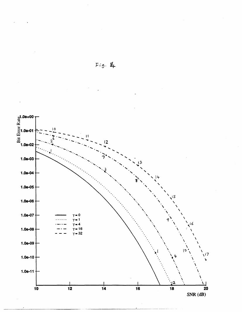
The expected value of X(^y) will be found in the next section. Figure 4 shows the

lower bound in (21) with the use of (34) of the next section. At each value of SNR (

and the phase noise strength y, the lower bound has been minimized with respect toM.

The overall error probability P, is obtained from P,(r) by removing the condition-

ing over r. If p,(r) denotes the probability density function of r, then we have

Pe = f Pe(r)pa(r) dr . (22)

Since r is a weighted average of i.i.d. random variables Xk as given by (20), the density

of r is given in terms of the density of Xk by an M-fold convolution. Then, we see

that the density of the phase noisy squared-envelope is again the only information we

need to obtain the error probability. The convolutions must be performed for each M

since the individual densities to be convolved correspond to the envelope with phase

noise strength 7/M. Therefore the computation becomes very costly with many

convolutions to be performed. We describe an alternative method which eliminates

9

the need for convolutions. From (19), the error probability can be written as

L--Pe = Er a, 2 e (23)

n=O 2/

where the coefficients an are defined as

2Mn! -k=n k- n 2 (24)

Using the sample average expression for r given in (20) one gets

M-1 m /

P, = E an E -,Xk (X(/MM) exp M k(/M)n=O k=12M k=1

Finally expanding the expression above in a multinomial sum and using the indepen-dence of the Xk we obtain

M-1 M n (25)

Pe = E an 2()M k !.. kM! ,a(ki) j . .(25)n=O k ,.kM

ki +-'-+kM=n

where

a(k) = E [Xk(Y/M)exp (-2 X(Y/M))] . (26)

The need for convolutions is eliminated by this expansion. All that is necessary

about the envelope is a set of tilted moments a(k). This reduces the computationsconsiderably as will be seen in Section 5. Further computational savings can be

obtained by observing that the inner summation in (25) contains many identicalterms: any permutation of an M-tuple (kl,k 2,...,kM) results in the same term.

Therefore the summation may be limited to ordered tuples with kl > k >... > kM

with the introduction of a scaling factor that counts the number of permutations.This scaling factor depends on how distinct the entries of the tuple are. If all theentries in a tuple k are distinct, then k has Al! permutations. If an entry ki is repeatedr(ki) times in k, then every distinct permutation has r(ki)! copies. Then, the scalingfactor with ordered indices is

N(k)=Nk-Ii r( ki )!

where the product is taken over i for which ki are distinct.

10

3 Phase Noisy Envelope and An Approximation

In the previous sections, we have seen that the squared-envelope of a phase noisysinusoidal plays a critical role in the performance analysis of the incoherent IF re-ception of heterodyne FSK system. This squared-envelope is the random variable X

defined in (9) which we repeat here for convenience:

XY = It ej(t) dt (27)

where we have removed the explicit argument 7 for notational simplicity. Due to itsimportance in the performance analysis, the determination of the probability den-

sity of X, or equivalently its moment generating function, has received considerable

attention. Foschini and his coworkers provided the first comprehensive treatment of

this problem in [3] and [9]. We summarize their approach below, since it is directlyrelated to our subsequent analysis.

Foschini et. al. expand the complex exponential into its power series and retain

the first order y terms. The resulting approximation, XL, is linear in -y and is given

by

L= 1 y [ 2 dt - ( dt). (28)

(We use the subscript L to emphasize the linear nature of this approximation.) Fos-chini et. al. expand $(t) in Fourier cosine series on (0, 1) and obtain

XL = 1 - 7Z TDz (29)

where z is an infinite dimensional vector of independent, identically distributed Gaus-

sian random variables with zero-mean and unit variance, and D is an infinite dimen-

sional diagonal matrix with dii = 1/(i7r) 2. Thus, zTDz is a compact notation forC 4=1z?/(iir) 2 . The moment generating function of XL is then found as [9]

MXL(S) E e sin= _ 2 ys (30)

and is inverse Laplace-transformed to obtain the density function of X in semi-closedforIll.

Equation (30) can be used in conjunction with (11) to obtain the error probabilityfor the single sample receiver with the linear approximation. The result is obtained

as

pc = ( ,7 < ' (31)o00( > 7'1r2

where the first case follows via sinh(jx) = j sin(x), while the second case followsfrom the derivation of (30) in [9]. It is seen that this approximation fails to give

sensible results at high SNR values. This is due to the fact that although X can

take values only between 0 and 1, XL can become negative. In fact, the density of

XL has a nonzero tail for negative arguments, which becomes increasingly dominant

as - increases. According to (31), this negative tail of the density function pxL(x)

decays exponentially, as exp(ir 2 x/2y) for x < 0, so that when ~ > 7r2/7 the integral of

e-~x/2pxL (x) diverges. This problem is not observed in the numerical results of [3] due

to the truncation of the negative tail of the probability density function. However, the

truncation weakens the analytical basis of the approximation: the truncated density

function is no longer a first order approximation to that of the actual envelope, this

introduces an uncertainty on the error probability results.

We seek a better approximation to the random variable X by forcing the rangeof the approximate random variable, say X, to match the range of X, namely (0, 1).Therefore we require a good approximation to satisfy

1. 0 < X(y) < 1 for all y > 0 and all Brownian sample paths +b(t),

2. X(7y) and X(y) match to the first order in -y for all #b(t).

The range constraint above suggests that X(-) can be written as

X(y) = exp [-G(I/y)]

where G is a functional whose domain is the set of functions defined on [0, 1] which

vanish at 0, and whose range is [0, oo). We force G to satisfy

1. G(f) > 0 for all f(t), with equality if and only if f(t) O0

2. G(f) = G(-f) for all f(t),

where the second property is due to the fact that the two sample paths Vb(t) and

-+O(t) result in the same value of X(7y). For X(y) and X(7) to be identical to the

first order in y, X(0) = X(0) and X'(0) = X'(0) must be satisfied. where 'prime'

denotes the first derivative with respect to y. We state one functional G(f) thatsatisfies these requirements in the following lemma.

Lemma 1: If G(f) = f f2 dt- (o f dt), then X(7) and Xy(7) are identical to

the first order in y.

12

Proof: Since X(0) = 1, G(0) = 0 is needed for X(O) = X(0). On the otherhand, it is straightforward, but somewhat lengthy, to show that

X'(0) = (l) dt) j_ 2 dt.

For a G that satisfies G(0) = 0,

X'(0) = ( i/7 ) ,=0.

It is easily seen that the functional given in the statement of the lemma satisfies both

of the requirements. E]

Note that the functional of the Lemma 1 satisfies the positivity and evennessconditions as well. Therefore the random variable XE defined as

XYE(-) exp(-7yTDz) (32)

with z and D as defined previously, promises to be a good approximation to X. Weuse the subscript E to denote the exponential nature of this approximation.

To summarize, we have obtained an approximation that retains the desirablefeature of that of Foschini et. al. while having the additional feature that it takesvalues that are in the same range as the original random variable.

A nice feature of the random variable XE is that its moments are easily obtained

from (30) as

y(t) - E(XE)

= - \/-2-yt-~ ~(33)sinh( /2--t)

for all real t > -ir 2 /27. For t < -7r2 /27, the t'th moment of XE is infinite.An indication of how well the two approximations model X is the behavior of the

first two moments as 7 varies. The moments of XE are already found in (33). Wenow evaluate the first two moments of X. Rewriting (27) as a double integral andtaking the expectation we obtain

E(X) = j j E{exp [j/i((t) - i(s))]} dtds.

Now we use the fact that VJ- (0(t)- ¢(s)) is Gaussian with zero-mean and variance7 t - sl and get

E(X) = exp(-y t- sI/2) dtds

= -[1--(1 -e/2)] (34)

13

The calculation of E (X 2 ) follows along the sanie lines: we first express X 2 as afour-fold integral, take the expectation and express the integrand as a Gaussian char-

acteristic function while observing the dependencies of the random variables. Wefinally obtain

E (X2) 16 It - 15 87 20 3921 1Ey( 2 ) =y 2 [2- a +e + e- ' /e (35)

The first two moments of X as given by Equations (34) and (35) are in agreementwith previous calculations of the mean and the variance in [10] and [13].

Finally we calculate the first two moments of XL (without truncation). The firstmoment is obtained as

E(XL) = 1--yE (ZTDz)

0 1

n=l (n1r)2

-= 1- 7 (36)6

and the second moment is obtained as

E (XL2) = 1-27E (ZTDz) + 7 2 E ((zTDz)2)

= 1- 2-yE +1 Ez E Ezn m)n=1 (n)2 n=l m=1 (nr) 2 (mr)2

00 3 00 1 1

3 n=1 (nn>4 nAm m=l (n7)2 (M,

-Y + -- 2

= 1- - + 20 (37)

where we have used E(z 4 ) = 3 and - '1-4 = r4/90 [15]. The first two moments

of X, XE and XL as given by Equations (33)-(37) are shown in Figure 5 as functionsof y. It can be seen from the figure that the moments of XL agree with those ofthe actual random variable X only for very small y while the moments of XE arevery close to the actual moments for all 7. Therefore we expect the e'xponential

approximation to be an accurate one.

4 Density of XE

The moments of XE as given by (33) provides complete information about its statis-tical behavior. In principle, one could compute the moment generating function of

14

XE from the moments {.t(n)} as

F(s) E (es) E (-)(n)

n=O

and find the density function as the inverse-Laplace transform. However, since the

series above is slowly converging, especially for large s, this is not an computationally

attractive approach. Instead, we use an indirect approach which is based on orthog-

onal polynomials for finding the density. We first prove the following about the value

of the density function at the origin.

Lemma 2: Let q(x) denote the probability density function of XE. Then q(O)

has the following property:

q(O) = oo if y < r2 /2 (38)

Proof: We prove the first part of the lemma by using Chernoff bound [16]. Wehave

q(O) = lim Pr(O < XYE < e)

From the definition of XE the probability above is

Pr(O < Xs < E) = Pr (ZDz >--n)

We now bound the right hand side by using the Chernoff bound on zTDz via (33) toobtain

Pr(O < XE < E)E/< sin( v/h)) for 0<s _ 2 /2.

Dividing both sides by e and taking the limit we obtain

q(O) < lim /- ( for O < s < r/2 .

The limit above is 0 if s/y > 1, which is possible for some s in the allowed range if

< 7r2/2. Since q(x) > 0, q(0) = 0.

For the second part of the proof, we use the fact that each of the random variables

in the series of zTDz are nonnegative to obtain the following lower bound.

Pr(O XE < e) = Pr (z r Dz> In > Pr r2 > ln~

15

The rightmost probability is 2Q(/-7r2 In E/y) where Q(x) is the complementary dis-

tribution function for the unit normal random variable. Proceeding as before we

obtain

q(O) > lim2Q - In .

Finally we use Q(x) - ,e-2 /2 as x oo [17] to obtain

q(0) > ?23 lim agg

The limit above is infinite if y > *r2/2y, this completes the proof. [o

The lemma above indicates that the density of XE changes its form as y exceeds a

critical value, 7r2/2. The left tail of the density, i.e. q(x) for small x, strongly affects

the probability of error, since P, is the integral of the product of q(x) (or convolution

of q(x) with itself) and some rapidly decaying function such as e - ~ /2. Therefore

the behavior of q(x) for x << 1 is of special interest for accurate calculation of error

probability. The following lemma indicates that this behavior is polynomial.

Lemma 3: q(x) = O (x`2-) for x small, where f(x) = O (g(x)) is equivalent to

limn,,o f(z)/g(x) = c for a positive finite c.

Proof: From (33) we have

(\/2/ sinh(O )) 1/2 t > O

J0,o aVq(t)da(= 2(yItj/sin( ti))1/ 2 0 > t >t >-r2/2700 t < -,r 2 /2 .

Since fo* x - / dx converges for i < 1 and diverges for f > 1 for any 5 > 0, we musthave

2 1x2-Tq(x) = c(x)-

for some function c(x) with finite and positive c(0), where we have assumed that q(x)is continuous at x = 0. Then the claim is proved. El

This lemma is in agreement with the previous lemma in predicting the value ofq(O). Moreover, it suggests that for accurate calculation of q(x) for small x it is better

to calculate the tilted density q(x)/xz -1. Before we describe a method to performthis calculation, we exploit a useful property of XE(y) that will enable us to computethe density function for a single value of y, say - = 1, and to obtain all other densityfunctions from this computed one. From the definition of XE(y) we have

¥E(,)I/7 = e-ZTDZ

16

Then for any positive -y and 72, the associated XE's satisfy

XE(nl)llY' = 'YE(2)1/72

which specifies a one-to-one mapping from YE(yI) to XE(72) via

g(x) = xY2/-1

Then the densities of the two random variables are related via [18]

) = g(g'-l())

where we introduced a subscript to the density function to emphasize its dependence

on y. Upon manipulation, we obtain

qT2(x) = ax'-- qyl(xa) (39)

where a = 71/ -Y2

The calculation of q(x) for a given -y, as will be seen shortly, is a computationally

intensive effort. Therefore the simple relation (39) introduces a big saving in the

required numerical work.

The moments of a random variable are the projections of its density function on

a sequence of polynomials. Therefore, the density can be reconstructed from these

moments via a complete orthonormal polynomial basis. The even (or odd) indexed

Legendre polynomials constitute such a basis on the interval (0, 1) [19]. Any piecewise

continuous function f(x) on (0, 1) that has left and right derivatives at every point

in the interval can be expressed as

f() = (2n + 1)FP,(x) (40)n=O

n even

where Pn(x) is the n'th Legendre polynomial and Fn is given by

Fn = f(x)P.(x)dx . (41)

Specializing to the case of

q(x)

where we have definedwhere we have defined

27

17

we obtain

, = E [XE P,(XE)] (42)

To obtain the coefficients F,, in terms of the moments, we first expand P,,(x) in itsTaylor series as [19]

P,(x) = ankx k (43)k=O

k even

where the coefficients ank are given by

1~k 'a 2n ((n k)/2 k

Now we can compute the expectation in (42) in- terms of the moments given by (33)as n

Fn = E a,kt(k - h) (45)k=O

k even

and, consequently, the density function as

00 n

q(x) = xh 5 (2n + 1)Pn(x) d ankI(k- h). (46)n=O k=O

n even }c even

The convergence of the series in (46) is quite fast. Note that the moments always

remain finite since k - h > -7r2 /2y for all k > 0. It is also worth mentioning thatalthough the formula above remains valid for any value of h, in particular for h = 0

which corresponds to the direct computation of q(x) without tilting, the value thatwe use is the most appropriate one because it captures the polynomial behavior of

q(x) in the small x region.

The results of the computation is shown in Figure 6 for various y values. Asexpected the density is more concentrated around unity for small -y. As -y increases,

the density gets flat until y = -r2/2 and becomes peaked at x = 0 thereafter. The

density function is observed to have a sharp decay around its x = 1 tail. In Appendix

C, we show that the nature of this decay is exponential in -y/(l - x), provided thatq(x) is bounded and analytic. (Boundedness holds for y < 7r2/2 and analyticity isassumed to hold.)

The density function of XE can also be calculated with another method. The

distribution function of the random variable zTDz is given in [3], from which the

distribution function of XE can be directly computed, the density function is then

18

obtained by differentiation. It was observed that this method yields results which are

in perfect agreement with Figure 6.

In the next section, we will use the density we have obtained to evaluate the

performance of the receivers under consideration.

5 Results and Discussion

The error probability for the single sample receiver is given by (11) as

P, j e-4x/ 2q,(z) dx .2 o

We have computed the error probability using this integral. The result of this com-

putation is shown in Figure 7. It is seen from this figure that the error probability

is above 10-4 for 7y > 2 and C < 22 dB. The single sample receiver can not combat

the phase noise effectively for large y, and the bit error rate severely degrades with

increasing phase noise strength.

The error probability calculation is more involved for the multisample receivers.

For the single-filter receiver, the error probability is given by (12) which can be written

as

P = exp(-~x/2M)q,/M(x) dx . (47)

Using (39) with 7y = a and 72 = 7/Al, we can rewrite (47) as

Pe = j exp(-$x/2M)MxM-1q,(xM) dx2 o

which with the change of variable y = xM yields

Pe = 1 j exp(-&yl/M/2M)q,(y) dy. (48)2 o

We want to find the value of M that minimizes (48). Since no closed form for q(.)

is available, this optimization involves evaluating this equation for M 1,2,3,...

until the optimum is reached5 . Equation (48) has the desired form since the density

function has the same parameter y for all Al.The result of the computation of the bit error rate via (48) is shown in Figure 8.

The plotted bit error rate values have been optimized over Ml. The optimal value

5In fact, we could search for optimal non-integer aiM for the single-filter receiver. This does not

seem to be necessary since the observed transitions with integer values were smooth.

19

of M increases with SNR and the phase noise strength. This is because as the SNR

increases the receiver prefers to use a smaller portion of the signal energy to reduce

the effect of the phase noise with the same factor.

Finally we focus on the performance of the double filter multisampling receiver. In

Section 2.2, we showed that the bit error rate for this receiver can be computed by firstfinding the M1-fold convolution of the density function of X( 7 /M) and then removingthe conditioning on r in Equation (19). However, the density function, ql/M(x),

changes with M, thus this method is computationally prohibitive. Therefore, we use

the alternative approach which resulted in Equations (25) and (26). One can further

reduce the complexity by expressing c(k) in terms of q,(x) as follows:

ct(k) = x k exp(-(x/2M)q,/M(x) dx

j yk/Mexp(-_yI/M/2Ml)qy(y)dy. (49)

where we have used the same transformation used in obtaining (48).

Equation (25) in conjunction with (49) provides a method for the error probability

computation. In performing the numerical computation the symmetry between theterms in the inner summation was exploited as outlined in Section 2.2. The resulting

computation is a very efficient one in comparison with the direct convolutions. The

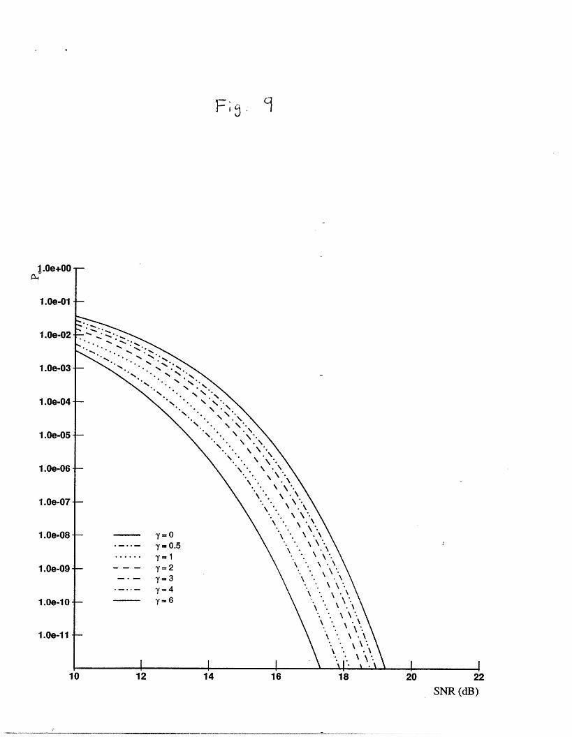
results are shown in Figure 9. The bit error rates are again optimized with respect to

M as in the single filter case. A comparison of the performance curves for the single

sample receiver and multisaImple receiver with and without double filtering reveals

that the increased receiver complexity by oversampling the signal and additional

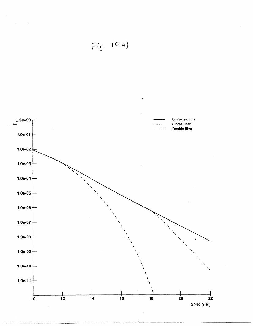
lowpass filtering may improve the error performance to a significant extent when thesignal-to-noise ratio is high and the phase noise is strong. This can be seen from

Figure 10 which shows the performance of the three receivers for a = 1 and y = 4.

For low SNR values (up to 12 dB for y = 1 and 9 dB for a = 4), the best receiveris the simplest one, i.e. the optimal value for the multisampling receivers is Ml = 1.

Only when the SNR is further increased, an increase in the receiver complexity is

warranted. At a bit error rate of 10-9 with y = 1, the double filter receiver has about

3.5 dB gain over multisample single-filter receiver and about 6 dB gain over the singlesample receiver.

The error probability for the double filter receiver is very close to the lower bound

obtained in Section 2.2, as illustrated by Figure 11 for y = 1 and y = 4. Therefore

20

the simple lower bound expression

Pe - P (4 [1 2M(1 - e-/2M)]) (50)

in conjunction with (19) provides a simple and reliable approximation to the proba-

bility of error. With the use of this closed-form result, the performance of a system

with a given SNR and phase noise strength can be found by a straightforward opti-

mization over M. It should be noted that the value of M that optimizes (50) is, in

general, lower than the exact optimal value. This is due to the fact that the variation

of r from its mean is neglected in the Jensen's bound that results in (50).

Since the phase noisy SNR r in (20) is the average of Al i.i.d. random variables,a Gaussian approximation for large SNR and phase noise strength is also plausible.

In fact, approximating the density of r with a Gaussian density on the interval (0, )

yields an error probability which is very close to that shown in Figure 9. However,

a closed-form result that is obtained by extending the range to the real line yields a

poor estimate due to the large negative tail of Pe(r).

The performance of the double-filter receiver as predicted by Figure 9 and approx-

imated by Equation (50) is very close to that predicted by Foschini and his coworkers

in [3]. This' is because the truncated density tail of the linear approximation to the

phase-noisy envelope is extremely low for a phase noise strength of -y/M, when M

is around the optimal value. This is in contrast with the single-filter case where the

agreement of our results with [3] is not as strong due to smaller values for the optimal

value of M.

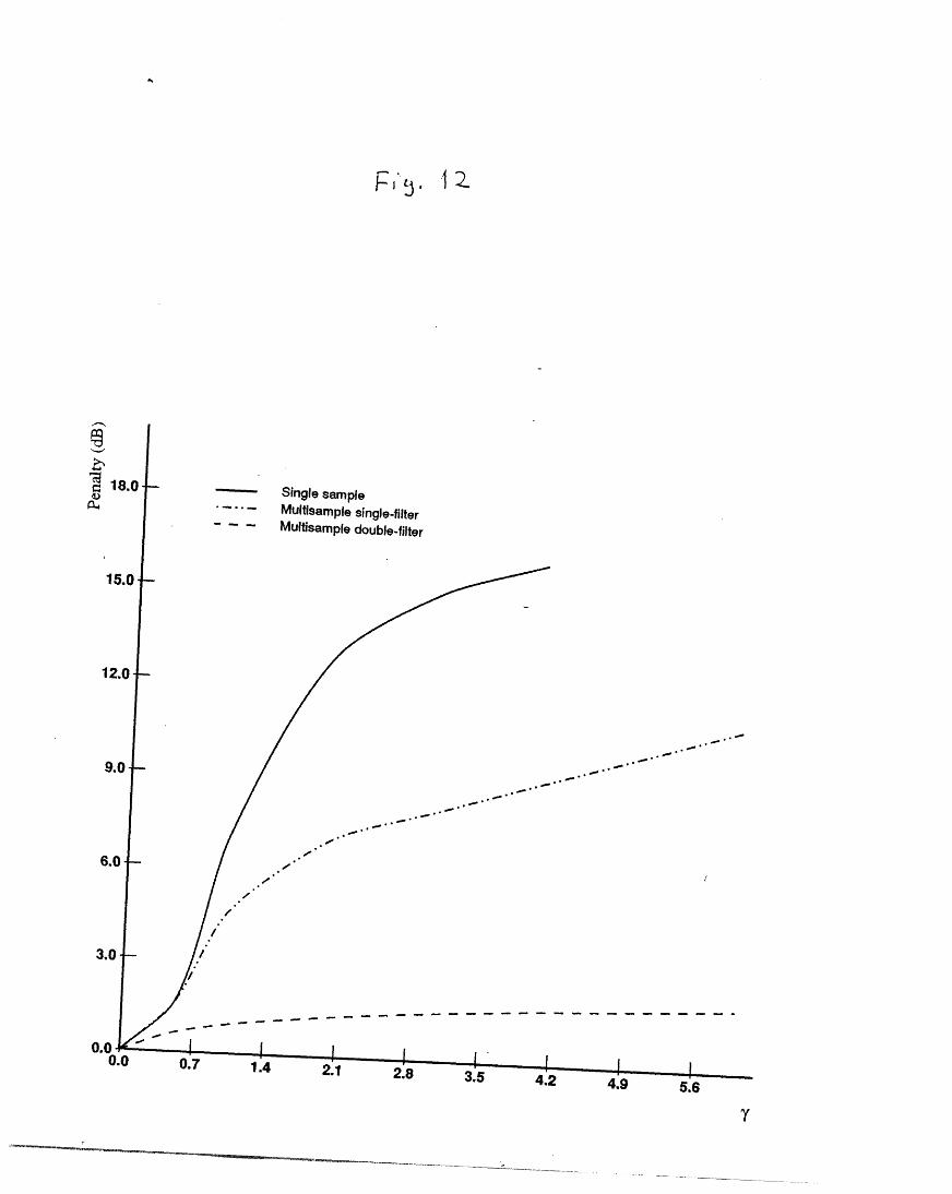
The signal-to-noise ratio needed to remain below a certain predetermined bit error

rate increases with the introduction of phase noise. The amount of increase in the SNR

is referred to as phase noise penalty. In Figure 12 the penalties for the three receivers

are shown as a function of 7 for a bit error rate of 10- 9. While the difference in the

penalties for the single sample receiver and the multisample double-filter receiver isless than 1 dB for 7 < 0.5, the latter receiver outperforms the former at higher phase

noise strengths. This is in support of increased receiver complexity that is tailored

towards combating the phase noise especially when y > 1.

Advancing optical technology promises fiber-optic networks with data rates in

excess of 100 Mbps per user and semiconductor lasers with linewidths of 5 MHz or

less. With these parameters, the phase noise strength y is in the range of 0.6 for

which the penalty is about 1 dB with the double filter receiver and 2 dB with the

single sample receiver. This means not only that the phase noise will not be a very

21

significant impairment on the bit error rate, but also that simple IF receivers will be

sufficient for most future applications.

6 Extension to N-FSK

The results of the previous sections about binary FSK can be extended to FSK with

N hypotheses (N-FSK) without much difficulty. The receiver structure is the same

as Figure 2 with the number of branches increased from 2 to N. We present an

analysis to the performance of N-FSK below. It must be emphasized that we hold

the transmission rate of data bits and the energy per data bit constant while making

comparisons among different N-ary FSK schemes, as in [20].

Let the possible hypotheses be 0, 1,..., N-1. Let the normalized filter outputs be

Vi, i = 0,1,. . , N- 1, and assume a "O" is transmitted. Then Vi will be independent

random variables with the density functions found from Section 2 as

~()p(voir) = (-2 e _)Im ( vo) tO > 0 (51)M-1

(vi) = (Ml)!e- ' vi > O i= 1,2,...,N-1. (52)

Let PN(r) denote the probability of a symbol error conditioned on the phase-noisySNR r. Since a symbol error will occur when any of the Vi for i ~ 0 is greater than

VO, we have

PN(r) = 1 - Pr(Vo > Imax{¼V,..., VN_llr)

= 1- f [Pr(V < vO)]N-1 p(voIr)dvo

where we have used the fact that Vi for i > 1 are i.i.d. conditioned on r. Then withthe use of (52), we obtain

PN(r) = I-J [1 - e vo p(volr) dvo

which does not seem to be easily brought to a closed-form similar to (19). Insteadof computing PN(r) numerically we will find upper and lower bounds in closed-form.We first use 1 - (1 - y)N-l < (N - 1)y for 0 < y < 1, to obtain

PN(r) < (N- 1) J E. e-vp(vlr) dvo = (N- 1)P2(r) (53)k= 2

22

where P 2(r) is the conditional error probability for binary FSK given by (19). Theupper bound in (53) is exactly the union bound. To obtain a lower bound to PN(r)

we use

1-(1-yl > (N - I)y -- 2 )y2

and we get

PN(r) > (N- 1)P2 (r) - (2 )gM(r)

where the function gM(r) is defined as

f/M-1 Vok 2

gM(r) = ( ik!e vo p(volr)dvo

To obtain gM(r) in closed-form we first use

M-1 k 2 M-1 M-1 n+m(E Vo e-t)vo e -2vo E E o

\ k=O n=O m=O

2(M-1) min(l,M-1) ()

and we get2(M-1)1

gM(r) = e-2" E p3vp(volr) dvo (54)1=0

where we have defined

'3:~~1 - ~E (k) ~(55)

We proceed exactly as in Appendix A to evaluate the integral in (54) to obtain theresult as

e-2r/3 2(M--1)( /3)n 2(M-1) t+ M 1

M(r 3M n=O n! i- n 31 (56)

which is quite similar to (19). i

We finally have the bounds to the conditional error probability as

(N-1)P 2(r) - N2 )gM(r) < PN(r) < (N - 1)P 2(r) (57)

in conjunction with Equations (19) and (56). Note that the two bounds are equal forN = 2. The bounds are tight for small N and large r. For N < 16 and r > 14 dB,the two bounds are within an order of magnitude for any M.

23

The symbol error probability PN is obtained as the expected value of PN(r) opti-

mized over M, i.e.PN = min E, [PN(r)]

M

Since only bounds to PN(r) are available in closed-form, we will perform the opti-

mization for the upper bound and use the optimal value of M, say M*, in the lowerbound. The result is

(N-)P 2 - (N)EIr [gM(r)] < PN < (N - )P 2 (58)

where P2 is the binary FSK error probability found in the previous section. The bit

error probability Pb is related to the symbol error probability as [12]

N/2Pb = N-- PN

N-i

which results in

N P2 N(N 2) Er [gM.(r)] < Pb < N P (59)2 4 2

The upper bound to the actual bit error rate reveals that for N-FSK at a bit SNR

value of r and a phase noise of 7y is at most N/2 times the bit error rate of binary

FSK at an SNR of ~ log 2 N and a phase noise strength of a log2 N. The expectation in

the lower bound can be computed without any convolutions, using the same method

described in the previous section. Figure 13 shows the upper and lower bounds toPb for N = 4,8, 16 as well as the binary bit error rate for y = 1. It is seen that the

bounds are very close, and that the bit error rate improves with increasing N. At

a bit error rate of 10-9 the improvement over binary FSK is 2.5 dB with N = 4,4 dB with N = 8 and 4.8 dB with N = 16. Since the cost of the receiver and the

bandwidth occupation are proportional to N, 4-FSK may be a desirable alternative

to binary FSK for this value of phase-noise strength.

7 Conclusion

We have analyzed the performance of a binary FSK coherent optical system with an

accurate treatment of the phase noise. We obtained closed-form expressions for the

error probability conditioned on a normalized phase-noisy amplitude. These resultscan be used in conjunction with other approximations or solutions to the phase-

noisy amplitude, e.g. the one given in [7]. -In this work, we used an exponential

24

approximation to the square of the amplitude which was found to be accurate. We

obtained the density of this approximation from its moments, which are available in

closed-form, via a Legendre series method. As a result, we were able to obtain the

performance of the receivers proposed in [3] with, we believe, more accuracy than in

previous work. We also provided a simple and tight lower bound in closed-form. Our

results show that the simple correlator receiver is adequate only for a certain range of

signal-to-noise ratio and phase noise values, beyond which receivers which track the

phase noise by oversampling improve considerably upon its performance.

We also extended the results to the case of N-FSK and obtained tight upper and

lower bounds to the bit error rate. As a result, we observed that increasing the signal

dimensionality may be desirable up to a certain limit to be robust against phase noise.

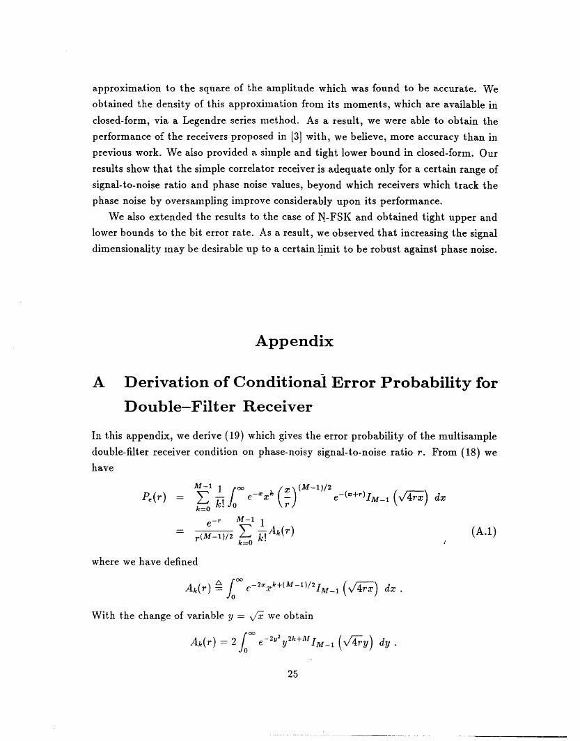
Appendix

A Derivation of Conditional Error Probability for

Double-Filter Receiver

In this appendix, we derive (19) which gives the error probability of the multisample

double-filter receiver condition on phase-noisy signal-to-noise ratio r. From (18) we

have

/Mlr-1 1 e-xk X-(')IM- 1 M4X/ dx

-r M-1

-r(M)/Ak(r) (A.1)

where we have defined

Ak(r) = j c 2 T+(M 1)/2 IXl (4rx) dx.

With the change of variable y = v/x we obtain

Ak(r) = 2 j e 2Y y2+ M 1 (V4y) dy.

25

The integral above can be found from 11.4.28 of [15] in conjunction with I/(x) =

j-"J,,(jx) as

Ak(r) = 2 (k + M) F(k + M, M, Mr/2) (A.2)2k+M J(M)

where F is the confluent hypergeomietric function. Equation (A.2) in conjunction

with (A.1) yields

M-1 1 r(k + M)Pe(r) = e-" 1 2k+Mk! Fr(M ) F(k + M,M,r/2) . (A.3)

k=O

Now we use the Kummer transformation (13.1.27) and the power series for a confluent

hypergeometric function (13.1.2) from [15] to simplify (A.3) via

F(k + M, M,r/2) = er/2 F(-k, M,-r/2)

= r/ 2 (-k). (-r/2)" (A.4)n=O (M) nr!

where (a)n = a(a + 1) - (a + n - 1). Since (-k)n = 0 for n > k the series above is

a finite series. Furthermore, since (-k)n = (-l)"lk!/(k - n)! for n < k and (M)n =

(M + 7t - 1)!/(M - 1)!, (A.4) becomes

/2 k k(M - 1)! (r/2) F (k + M, M, r/2) = eI/ 2- (A.5)

n=O (k - n)!(M - 1 + n)! n!

Inserting (A.5) into (A.3), using 1(k) = (k - 1)! and canceling the common terms,

we obtaine -r/2 M-1 1 k (k + M - 1)! (r/2)n (A.6)

P(Tr) = 2 k=o 2k n=o (k- n)!(M - 1 + n)! n!

which upon interchange of summations yields (19)

B Convexity of Conditional Error Probability

In this appendix we prove that the error probability conditioned on phase-noisy SNR,

Pe(r), is a convex function of r. From (19), we have

Pe(r) = e 2 c:( l -1 (B.1)

where

Cn(M-1) (k + )l 21 (B.2)

26=

Since the convexity of a function is not affected by multiplication by a positive con-stant and a scaling of its argument, it suffices to show the convexity of the function

h(r) = e-rt(r)

where t(r) is the polynomial of degree M - 1 with coefficients cn(M - 1)/n!. Thesecond derivative of h(r) is

h"(r) = e-' [t(r) - 2t'(r) + t"(r)]

where "prime"s denote derivatives. Thus, Pe(r) is convex if and only if the polynomial

p(r) = t(r) - 2t'(r) + t"(r) (B.3)

of degree M - 1 is nonnegative for all r > 0. The latter will be satisfied if all thederivatives of p(r) at r = 0 are nonnegative, by Taylor's theorem. The n'th derivativeof p(r) at r = 0 is given as

p(n)(0) = t()(0)- 2t(n+l)(0) + t(n+2 )(0)

= Cn(MI- 1) - 2c+l(M - 1) + c+ 2 (M - 1)

Let N = M - 1 and d,(N) = c,(N) - c,+l(N) for n = 0,1,..., N. Then we have

p(n)(0) = dn(N) - dn+(N) . (B.4)

Thus, we need to show that the coefficients d,(N) are nonincreasing in n for everyN. To do this, we need an intermediate result given in the following lemma.

Lemma B.1 The binomial coefficients satisfy

for J = 0,1,2,... and j = 0, ,...,J.

Proof: We will use induction on J. For J = 0, the claim is obviously true. For

J = 1, the claim is easily verified for both j = 0 and j = 1. Now let's assume that

the claim is true for J and for all j < J. We will show that this implies that the

claim is also true for J + 1 and for all j < J + 1. Let aj(J) denote the left hand side

of (B.5). For 0 < j < J, we have

j+1 / fu /

aj+l(J + 1) = Z2k + 1 -k=1 + I+27

27

= 2ai(J) + 1)

2Z (J+ 1) + j+

(° kO [(k )+k + I

1J + 28k=O

which is the desired result. (The second equality above follows by a change in the

index of summation, the third one follows by induction hypothesis, the fourth one is

a simple rearrangement of terms and the last one follows by the well-known property

of the Pascal triangle.) Finally ao(J + 1) = 1 trivially satisfies (B.5). Thus the claim

is true for all j < J + 1. This completes the proof by induction. O

A corollary to Lemma B.1 provides a closed-form to d,(N).

Corollary The difference coefficients d,(N) satisfy

d(N) -2N- ( S- n = 0, 1,..., N. (B.6)

Proof: From (B.2) we have

N Iik + N2NCn(N) = 2N-k (k

k=n

N- 2N-l=E 2' -N I

1=0

where we have used a change of index 1 = N - k. Now we use Lemma B.1 with

J = 2N and j = N - n to get

1 N-n 2N+ 1C,(N) = 2N N +I

which results in

dn(N) = c,,(N)-c,,+l(N)

N 2N + 1-

as claimed. [

28

As a result of this corollary, we see that for a fixed N, d,(N) are decreasing with

n for 0 < n < N. This means that the polynomial p(r) is nonnegative for r > 0,

and consequently that the conditional error probability Pe(r) is convex for any M, as

explained before.

An implication of the convexity of Pe(r) is that the conditional error probability

can not be improved by time-sharing between two phase-noisy SNRs r1 and r2, since

Pe(Arl + (1 - A)r2 ) • AP,(ri) + ( - A)P,(r2) for all 0 < A < 1.

C Tail Behavior of q(x)

In this appendix we concentrate on the decay properties of the density function q(z)

around its x = 1 tail. We prove that this decay is exponential as described in the

following property.

Property: The density function q(x) has an exponential decay around x = 1,

characterized as

lim (1 - x)ln q(z) = -y/8 . (C.1)

To prove this property we need two lemmas. We first define a transformation

which is closely related to Mellin transform [21].

Definition: The moment transform of a function f(x) defined on (0, 1) is given

by

F(t) = jl X tf(x) d (C.2)

where t > 0.

It can be observed that for any bounded, continuous function the moment trans-

form exists, and that it vanishes as t - oo. The behavior of a function in its x = 1

tail is related to the asymptotic behavior of its moment transform. The following

lemma formalizes this notion.

Lemma C.1 Let f and g be two bounded, analytic functions on (0,1) whose

moment transforms satisfy F(t) < G(t) for all t > to. Then there exists e > 0 such

that f(x) < g(x) for all x > 1 -e.Proof : Let h = g - f. h is bounded and analytic with moment transform

H = G - F. Since h is analytic, there is a neighborhood of 1 in which h does not

change sign, say (1 - 6, 1) for some 6 > 0. Let

A = max{Ih(x) ·: x E (0,1)}

B = (x) dx .

29

Suppose h(x) < 0 on (1 - 6, 1). Then the following inequalities hold,

J X1- (x) dx < j1 x t lh(x)l d < A )

-1- t+l

/_ z th(x) dx < (1- )tB,

which implies

H(t) < (1 )t [ A(l - 6) + B . (C.3)

However, since A > 0 and B < 0, t can be made large enough to make the right hand

side of (C.3) negative. This is a contradiction, since H(t) > 0 for all t > to. The

proof is complete with the choice of an e with 0 < < 6. El

The following lemma establishes a relation between the moment transform of a

function and the Laplace transform of its x = 1 tail.

Lemma C.2 Let f be a bounded function on (0, 1) and let f, be defined as

f _ f(M-X) O<X<<e()O otherwise

for 0 < e < 1. If QE(t) is the Laplace transform of f,(x) and F(t) is the moment

transform of f(x), then Q,(t) ~ F(t) for large tand small e.

Proof: Q,(t) is defined as

Qe(t) f f(1 -x)e - t' dx

With small e we use e - ti - (1 - x)t for 0 < x < E, to obtain

Qe(t) i j f(1-2x)(1-x)t dx = j f(x)x t dx.

Since xt becomes smaller in the interval (0, 1-e) with increasing t, the rightmost inte-

gral will be arbitrarily close to F(t) for large t. Therefore, the quantity IQE(t) - F(t)I

can be made arbitrarily close to 0 for sufficiently small e and large t. O

With these two lemmas at hand we now proceed with the proof of the property

stated at the beginning of this appendix.

Proof of Property : Lemma C.2 states that the tail of the density function q(x)

around x = 1 can be found as the inverse Laplace transform of its moment transform

for large arguments. The moment transform, jt(t), of q(x) is given by (33) and can

be written as

l(t) = (1 /- e - -3/2

30

For large t, the first factor is bounded between 1 and A't. Thus, for large t we have

e- / 2 < Ltt(t) < Vte - ' y/2 -2 (C.4)

Then from the two lemmas we proved, the function q(1 - x) for small x will be

bounded by the two functions whose Laplace transforms yield the bounds in (C.4).

With the use of Formula 29.3.82 of [15] we obtain

8y 3 e-Y/8y < q(1 - y) < 8y 3 )e

for small y, which upon substitution of x for 1 - y becomes

i' e-/8(l-) < q(x) < 8r(1 -)3 (4(1 - ) (C.5)

for x close to 1. We observe that the dominant tail behavior of q(x) is exponential in

(-3y/ 8 ( 1 - x)). Equivalently, by taking logarithms of all sides in (C.5), we obtain

lim (1 - x)ln q(x) = - (C.6)x-al-~ 8

where we have used lim,,.O0 x In x = 0. This completes the proof. O

31

List of Figures

Figure 1: The optical heterodyning receiver.

Figure 2: The IF receiver, a) Front end (AM = 1 for the single sample receiver),

b) Processing of samples for single sample and single-filter receivers, c) Processing

of samples for the multisample double-filter receiver.

Figure 3: Error probability of the double-filter receiver (Pe(r)) conditioned on the

phase-noisy signal-to-noise ratio r.

Figure 4: Lower bound on the error probability obtained by Jensen's inequality.

Figure 5: Comparison of statistics of the phase-noisy squared envelope and its

linear and exponential approximations, a) Means, b) Second moments.

Figure 6: Probability density function, q(x), of the exponential approximation XE

for various y values: a) y = 0,0.5,1,2,3,4 b) 7 = 4,6,16.

Figure 7: Error probability of single sample receiver as a function of signal-to-noise

ratio.

Figure 8: Error probability of multisample single-filter receiver as a function of

signal-to-noise ratio (optimal values of M are shown on the data points).

Figure 9: Error probability of multisample double-filter receiver as a function of

signal-to-noise ratio.

Figure 10: Comparison of the bit error performances of the three receivers under

consideration, a) a = 1, b) y = 4.

Figure 11: A comparison of the exact and approximate bit error probabilities for

a = 1 and a' = 4. The respective optimal values for M are also shown.

Figure 12: Penalty in signal-to-noise ratio with respect to the case with no phase

noise at a bit error rate of 10 -9 .

Figure 13: Upper and lower bounds to the bit error probability for N-FSK with

7 = 1 and N = 2,4,8, 16.

32

References

[1] C. H. Henry, "Theory of linewidth of semiconductor lasers," IEEE Journal ofQuantum Electronics, vol. QE-18, pp. 259-264, February 1982.

[2] J. Salz, "Coherent lightwave communications," AT&T Technical Journal, vol. 64,pp. 2153-2209, December 1985.

[3] G. J. Foschini, L. J. Greenstein, and G. Vannucci, "Noncoherent detection ofcoherent lightwave signals corrupted by phase noise," IEEE Transactions onCommunications, vol. COM-36, pp. 306-314, March 1988.

[4] G. J. Foschini, G. Vannucci, and L. J. Greenstein, "Envelope statistics for filteredoptical signals corrupted by phase noise," IEEE Transactions on Communica-tions, vol. COM-37, pp. 1293-1302, December 1989.

[5] L. G. Kazovsky, "Impact of laser phase noise on optical heterodyne communi-cations systems," Journal of Optical Communications, vol. 7, pp. 66-77, June1986.

[6] I. Garrett and G. Jacobsen, "Phase noise in weakly coherent systems," IEEProceedings, vol. 136, pp. 159-165, June 1989.

[7] I. Garrett, D. J. Bond, J. B. Waite, D. S. L. Lettis, and G. Jacobsen, "Impact ofphase noise in weakly coherent systems: A new and accurate approach," Journal

of Lightwave Technology, vol. 8, pp. 329-337, March 1990.

[8] L. G. Kazovsky and 0. K. Tonguz, "ASK and FSK coherent lightwave systems:A simplified approximate analysisj" Journal of Lightwave Technology, vol. 8,pp. 338-352, March 1990.

[9] G. J. Foschini and G. Vannucci, "Characterizing filtered light waves corrupted byphase noise," IEEE Transactions on Information Theory, vol. IT-34, pp. 1437-1448, November 1988.

[10] L. G. Kazovsky, P. Meissner, and E. Patzak, "ASK multiport optical homodynesystems," Journal of Lightwave Technology, vol. 5, pp. 770-791, June 1987.

[11] W. C. Lindsey, "Error probabilities for rician fading multichannel reception ofbinary and N-ary signals," IEEE Transactions on Information Theory, vol. IT-10, pp. 339-350, October 1964.

33

[12] J. G. Proakis, Digital Communications. New York: McGraw-Hill, 1983.

[13] J. R. Barry and E. A. Lee, "Performance of coherent optical receivers," Proceed-ings of the IEEE, vol. 78, pp. 1369-1394, August 1990.

[14] S. M. Ross, Stochastic Processes. New York: John Wiley & Sons, 1983.

[15] M. Abramowitz and I. A. Stegun, Handbook of Mathematical Functions. New

York: Dover, 1972.

[16] R. G. Gallager, Information Theory and Reliable Communication. New York:

John Wiley & Sons, 1968.

[17] H. L. Van Trees, Detection, Estimation, and Modulation Theory. New York:

John Wiley & Sons, 1968.

[18] A. Papoulis, Probability, Random Variables and Stochastic Processes. New York:

McGraw-Hill, second ed., 1984.

[19] R. V. Churchill and J. W. Brown, Fourier Series and Boundary Value Problems.

New York: McGraw-Hill, third ed., 1978.

[20] L. J. Greenstein, G. Vannucci, and G. J. Foschini, "Optical power requirementsfor detecting OOK and FSK signals corrupted by phase noise," IEEE Transac-tions on Communications, vol. COM-37, pp. 405-407, April 1989.

[21] G. Arfken, Mathematical Methods for Physicists. Academic Press, 1985.

34

Received Photo IF Signal

Optical t Detector r(t

Signal /L

Local

Oscillator

FrI. 1

cos(2irfot)

t = kT'

Yo,I

r(t)

cos(27rfit)

t= kT'

sin(2wrf t)

a)

YO,M m ChooseData

yl, mLarger OutYt,M

b)

Choose Data

Larger

F~k~s· aac)

.o.0+0 -

1.0e-01

1.0e-02 -

1.0e-03 . "

1.08-\ .0 '-

1.0e-06 - -

1.0e-04 _- .. - M-1 M12 \ '. \\...... M \

M-41.0e-08 - - - M.8 \ '. X

1.0e-09 * \ -

1.0e-10 \ \ \

1.Oe-11 \ '* \ \

10 12 14 16 18 20

r(dB)

1 .Oe+00

1.0e -01 -"" . ' ~ " " I 1

1.0e-02 .'.

1.00-03 *-3 *

1.0e-04. .

1.Oe-05

1.00-06 '. 3 '

1.0e07 -- " ".\ \...... .. m_1 \ .

_ y 32 \ *. \* 1.0v09t·\ .-. \- . \

1.Oe-019 \*.1.06e-- . \ \

·.O \ *- *-

· . .. \ 2 : .

10d 12 14 16 18 20

SNR (dB)

1.0.- -- ExactLinear appr.

-W - -- Exponential appr.

0.8

0.6.

0.4

0.2

0.0I I "1 I0.0 2.0 4.0 6.0 8.0 10.0

1.0-

0.8-- - Exact.. ·...... Linear appr.

Exponential appr.

0.6

0.4

0.2

0.0 I I I I0.0 2.0 4.0 6.0 8.0 10.0

8.0~"~x~"""~-"~~~~-~--------~ 10.0 Ip

3!.Oe+01 _

1.Oe+00 ,-

... -1.....* - _.' \ I

toe0 - - -I-

1.0e-0 L 0 I~~~~. 0./.·. . .II.

1.0e-04 , \ I

0 r~~.. I:,

./ - - -ii'

1.0e-03 -7iI· /~~~~~~~~~~~~

L)

1.0e+01

1.0e+00

1.0e-01-

1.00-02i\ \

1.Oe-04- ' .-'-

1.0e-05 -- 4 l I

y-16

1.0e-06-

1.0e-07- - I

0.0 0.2 0.4 0.6 0.8 1.0

.Oe+00 -

i.0e'.'_:\' .. ..

\l s., -_

1.Oe-05' ..... 1.006 --

1.0.-09 ` `

1.Oe-03 _ " _ . \ · -- -.

._0. .1.0e-085-_ -- - \

1.0e-10 -- *

1.Oe-11 .\ * \ 4

0 12 14 16 18 20 2

SNR (dB)y~~~~~~~~~~~l~s, ~

Fg '

.0e+00

! \:.. 3-,

1.0se-0 _- -. Oe-06 . .·1.0e0O ... 2. -3. .

1.0e-0_ _- - 0. \ -

I .Oe.04 - -- S

ym4 N%'.\ '... . '1.0e-06 \ - '

10 1o2 14 16 1 20 22

1.0e-11

10 12 14 16 18 20 22

SNR (dB)

F,99 q

j.oe~oo['.Oe+00 -

l.Oe-02 -

1.0e-03 - "

1.0e-045- - ' ,, '..' ,X',: \

1.0e-0 \ .- -

1.0e-07 - -

\ .'-\\\\\ ·1.0e-08 -- O \'- \ \\

...... \..,.. 1\* -\.\1.0e-09 - _ _ _ y 2 .\ \ . \- - ,30 .5 y = 3

- -=41.0e-10 _6 \ * *

\ *-\.--\"\\=

1.0e-11 - \ \ \\"\". ·\·.. \\-

10 12 14 16 18 20 22

SNR (dB)

E%. 0 ci)

.Oe+00 - - Single sample.... * - Single filter

Double filter

1.0e-01 -

1.0e-02 -

1.Oe-03

l.Oe-04 - -

1.Oe-05 - X

1.e-06

1.Oe-07 _-

1.0e-08 - \ '-\ '.

1.0e-09 --

1.Oe-10 \-

1.Oe- 11 _

10 12 14 16 18 20 22

SNR (dB)

.. Oe+00 - Single sample:~Pc~~~~~~~~ I ·- · ·- ~~~~~~~~~~~~~ Single filter

Double filter1.0e-01

1.0e-02 _-- O

1.0e-03 -

N \ %1.Oe-04 --1.Oe-05 - \

1.0e-06- -

\

1.0e-08 7

1.0e-09 -

1.0e-10

1.0e-11 _ \

10 12 14 16 18 20 22

SNR (dB)

I.Oe+00

1 .Oe-Ol

1.Oe-01 --

1.Oe-03 - -

1.0e-04-

1.Oe-05 - -

1.0e-063 -

1.Oe-07-

1.Oe-08- - Y-

1.Oe-09 --\\

1.0e-10 - \

1.0e-11

I ~ ; | | - 2\ \ \\

10.0 12.0 14.0 16.0 18.0 20.0 22.0

SNR (dB)

18.0 Single sample* - . ...Multisample single-filter

- Multisample double-filter

15.0

t 2.0

9.0 -,

6.0

3.0 0- /

0.0 .1 0.0 0.7 81.2.1 2.8~~

1.0e-02 - N2- - N-4

N-8N-16

1.Oe-03

1.0e-04 - \-

1.0e-05 -

i .Oe-O06 - \

1.0e-07 \ \

1.0e\ \08

1.0e-09 - \

1.Oe-10 \ \

1.0e-11 \

lo 12 14 16 18 20 22

Bit SNR (dB)