enumeration by algebraic combinatorics 1. introduction

ENUMERATION BY ALGEBRAIC COMBINATORICS

CAROLYN ATWOOD

Abstract. Polya’s theorem can be used to enumerate objects under permutation groups. Using group

theory, combinatorics, and many examples, Burnside’s theorem and Polya’s theorem are derived. The

examples used are a hexagon, cube, and tetrahedron under their respective dihedral groups. Generalizations

using more permutations and applications to graph theory and chemistry are looked at.

1. Introduction

A jeweler sells six-beaded necklaces in his shop. Given that there are two different colors of beads, how

many varieties of necklaces does he need to create in order to have every possible permutation of colors?

Figure 1. A six-beaded necklace.

Consider the case of three beads of each color. Mathematically, there are(

63

)= 6!

3!3! = 20 ways to string

three light gray beads and three dark gray beads onto a fixed necklace. However, we can rotate or reflect

the three necklaces in Figure 2 to create all 20.

Figure 2. The set of necklaces with 3 dark beads and 3 light beads that are distinctunder rotation, reflection, and inversion of the colors. In other words, these necklaces areequivalent when the colors are permuted by groups D12 and S2.

Given 6 beads we have 2 choices of color per bead, so there are 64 ways to color an unmovable beaded

necklace. However, if we are given the freedom to rotate and reflect it, there are only 13 distinct varieties.

Furthermore, if the colors are interchangeable (i.e. a completely light necklace is equivalent to a completely

dark necklace), then there are only 8 distinct arrangements.1

How can we get from 64 down to 13 or 8? We might guess that it has something to do with symmetry.

The hexagon has 12 symmetries: rotation by 0, 60, 120, 180, 240, or 300 degrees, three reflections through

opposite vertices, and three reflections through opposite sides. There is no obvious relationship between the

number of possibilities for a fixed necklace, the number of symmetries, and the number of distinct varieties,

but surely there is one. In this paper, we use combinatorics and group theory to work through the problem

of the six-beaded necklace and others like it.

2. Burnside’s Theorem

We begin by examining the number of possible n-colored necklaces and cubes under symmetry. We solve

simple enumeration problems by observation, claim that the results hold for more complicated examples,

then prove our claim algebraically. The result that we observe by counting cubes was popularized by William

Burnside in 1911, though he quotes it from a paper published by George Frobenius in 1887 [3]. The theorem

was also known to Augustin Cauchy in an obscure form by 1845. [4]

2.1. Basic Abstract Algebra. First, we give abstract algebra background necessary to describe an

enumeration problem solvable by Burnside’s theorem.

Definition 2.1. (Binary Operation [3]) Let G be a set. A binary operation on G is a function that assigns

each ordered pair of elements of G an element of G.

Definition 2.2. (Group [3]) Let G be a nonempty set together with a binary operation that assigns to each

ordered pair (a, b) of elements of G an element in G denoted by ab. We say that G is a group under this

operation if the following three properties are satisfied.

(1) Associativity. The operation is associative; that is, (ab)c = a(bc) for all a, b, c ∈ G.

(2) Identity. There is an element e (called the identity) in G such that ae = ea = a for all a ∈ G.

(3) Inverses. For each element a ∈ G, there is an element b ∈ G (called an inverse of a) such that

ab = ba = e.

Example 2.1. A simple example of a group is the integers under addition modulo 4. In this case,

Z4 = {0, 1, 2, 3}.

Addition mod 4 is a binary operation (the group is closed) since 0 + 0 = 0, 0 + 1 = 1, 0 + 2 = 2, 0 + 3 = 3,

1 + 1 = 2, 1 + 2 = 3, 1 + 3 = 0, 2 + 2 = 0, 2 + 3 = 1, and 3 + 3 = 2. We need not check the operations in

the other direction since addition is commutative. The group has an identity of 0, and each element has a

unique inverse: 0−1 = 0, 1−1 = 3, 2−1 = 2, and 3−1 = 1.2

2.2. 6-Beaded Necklace. We describe the symmetry of a 6-beaded necklace, or hexagon. Symmetry is the

property that an object is invariant under certain transformations. The 6-beaded necklace is symmetric in

12 ways as shown in Figures 3, 4, and 5.

• The rotations of the necklace counterclockwise about its center by 0o, 60o, 120o, 180o, 240o, or 300o

(the rotation by 0o is the identity), denoted I, R60, R120, R180, R240, and R300,

1

2

3 4

5

6 2

3

4 5

6

1 3

4

5 6

1

2

4

5

6 1

2

3 5

6

1 2

3

4 6

1

2 3

4

5

Figure 3. The rotations of D12.

• The reflections across the diagonal through each of the 3 pairs of opposite vertices, denoted D1, D2,

and D3,

1

6

5 4

3

2 3

2

1 6

5

4 5

4

3 2

1

6

Figure 4. The reflections across the diagonals of D12.

• The reflections across the side bisector for each of the 3 pairs of opposite edges, denoted E1, E2, and

E3.

6

5

4 3

2

1 2

1

6 5

4

3 4

3

2 1

6

5

Figure 5. The reflections across the side bisectors of D12.

3

D12 I R60 R120 R180 R240 R300 D1 D2 D3 E1 E2 E3

I I R60 R120 R180 R240 R300 D1 D2 D3 E1 E2 E3

R60 R60 R120 R180 R240 R300 I E2 E3 E1 D1 D2 D3

R120 R120 R180 R240 R300 I R60 D2 D3 D1 E2 E3 E1

R180 R180 R240 R300 I R60 R120 E3 E1 E2 D2 D3 D1

R240 R240 R300 I R60 R120 R180 D3 D1 D2 E3 E1 E2

R300 R300 I R60 R120 R180 R240 E1 E2 E3 D3 D1 D2

D1 D1 E1 D3 E3 D2 E2 I R240 R120 R60 R300 R180

D2 D2 E2 D1 E1 D3 E3 R120 I R240 R180 R60 R300

D3 D3 E3 D2 E2 D1 E1 R240 R120 I R300 R180 R60

E1 E1 D3 E3 D2 E2 D1 R300 R180 R60 I R240 R120

E2 E2 D1 E1 D3 E3 D2 R60 R300 R180 R120 I R240

E3 E3 D2 E2 D1 E1 D3 R180 R60 R300 R240 R120 ITable 1. The Cayley Table of D12. Each entry in the table represents an operation in rowcomposed with an operation in a column.

We claim that these transformations form a group, called the dihedral group of order 12, denoted D12.

From the completeness of Table 1, the Cayley table of D12, D12 is closed under function composition. Notice

that the element I is the identity of D12 since every element composed with I is equal to itself. Also, every

row of the table contains one I, so Theorem ?? holds, or each element has an inverse. Since all of the

properties of Definition 2.2 hold, the symmetric transformations of a 6-beaded necklace does indeed form a

group.

Next we examine the symmetric transformations on the numbered necklaces and notice that not every

group operation affects every coloring of every necklace. For example, consider R120. If we start with the

pattern (123456) and apply R120, we get (345612), then applying R120 again, we get (561234). If we continue

to rotate by 120o, the pattern repeats. Therefore, this coloring remains the same under R120 as long as beads

(135) are the same color and beads (246) are the same color. If our necklace can contain two colors of beads,

then we say that we have two choices of color for each set of fixed beads, so we have 22 possible arrangements

fixed under R120.

The colorings fixed under each transformation are described in Table 2. Notice that the number of the

total choices under all symmetries of two colored necklaces is 156. When we divide 156 by 12 (the number of

symmetries), we get 13. By observation, there are 13 varieties of 2-colored necklaces that are different when

the symmetries are applied: three choices where there are 3 beads of each color as shown in Figure 2 and

ten more choices shown in Figure 6. In contrast, there are 26 = 64 possibilities for necklaces upon which we

cannot apply a symmetric transformation.

2.3. Cube. The next question that we tackle is,“given a cube that is painted dark on some faces and light

on the others, keeping symmetries in mind, how many different possible varieties are there?” To answer this4

Transformation φ in D12 Colorings Fixed (fix(φ)) Number (|fix(φ)|)Identity All 6 separately 26 = 64Rotation of 60o All 6 as a unit 21 = 2Rotation of 120o Beads 1,3,5; Beads 2,4,6 22 = 4Rotation of 180o Beads 1,4; Beads 2,5; Beads 5,6 23 = 8Rotation of 240o Beads 1,3,5; Beads 2,4,6 22 = 4Rotation of 300o All 6 as a unit 21 = 2Reflection across diagonal 1 Bead 1; Beads 2,6; Beads 3,5; Bead 4 23 = 8Reflection across diagonal 2 Bead 2; Beads 1,3; Beads 4,6; Bead 5 23 = 8Reflection across diagonal 3 Bead 3; Beads 2,4; Beads 1,5; Bead 6 23 = 8Reflection across side bisector 1 Beads 1,6; Beads 2,5; Beads 3,4 24 = 16Reflection across side bisector 2 Beads 1,2; Beads 3,6; Beads 4,5 24 = 16Reflection across side bisector 3 Beads 1,4; Beads 2,3; Beads 5,6 24 = 16

Total Sum 156Table 2. The elements of D12, or the symmetries of a 6-beaded necklace, and the numberof colorings fixed by each element of D12.

Figure 6. The set of necklaces with 0, 1, or 2 beads of one color.

question, we define a possibility as the number of ways to color a fixed cube and a variety as the number of

ways to color a cube that is free to rotate along its axes of symmetry. We create models of all the varieties

and then explain the results mathematically. The results, by observation, are summarized in Table 3.

Given that a cube has six faces and two possible colors for each face, it is not a surprise that there are

26 = 64 possibilities. How do we apply some function to the cube and get from 64 to 10?

A cube has 24 unique rotational operations about its lines of symmetry as shown in Figures 7, 8, 9, and

10.

• I

The first is the identity operation, or any rotation of zero degrees.

• F 901,2,3, F 180

1,2,3, F 2701,2,3

Next are rotations of 90, 180, and 270 degrees about the three lines of symmetry that go from the

center of one face to the center of the opposite face.5

Light Gray Dark Gray Possibilities Varieties

6 0(

60

)= 1 1

5 1(

61

)= 6 1

4 2(

62

)= 15 2

3 3(

63

)= 20 2

2 4(

64

)= 15 2

1 5(

65

)= 6 1

0 6(

66

)= 1 1

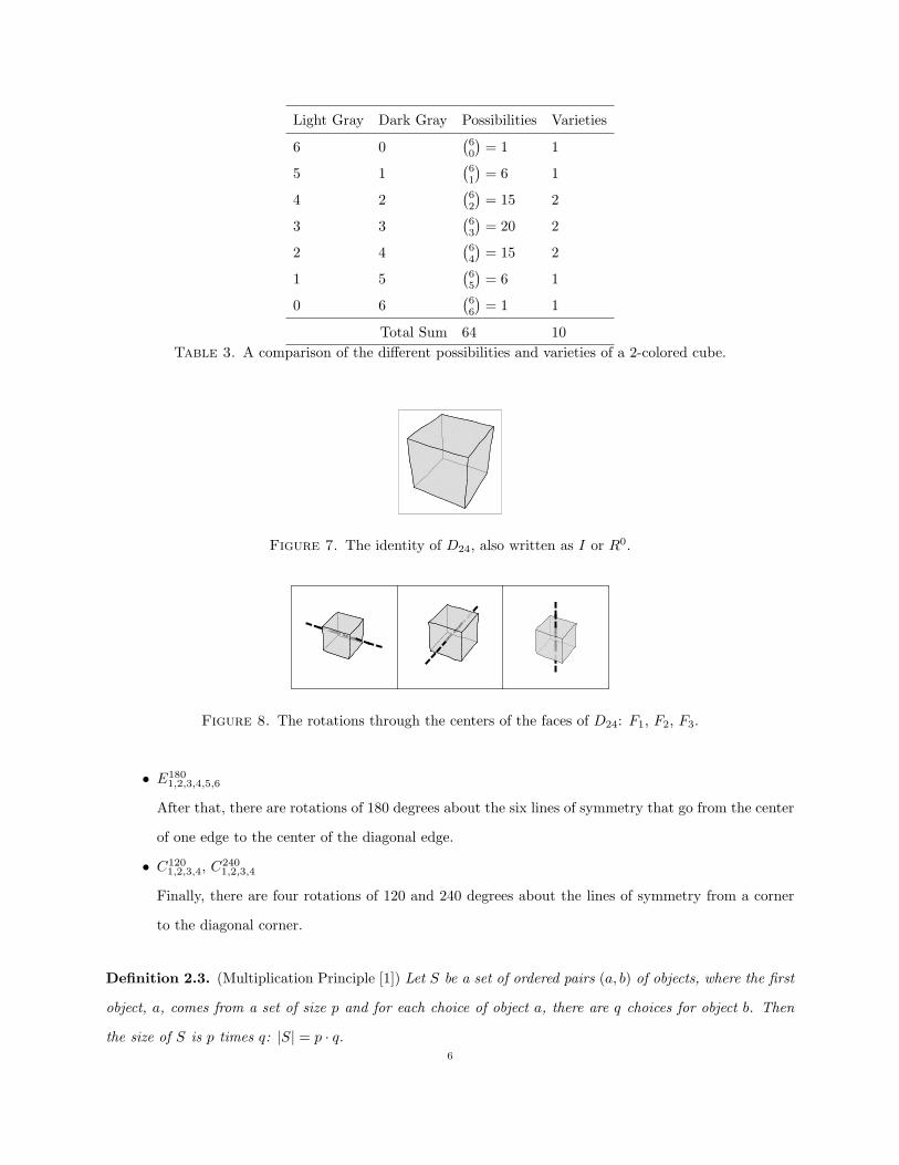
Total Sum 64 10Table 3. A comparison of the different possibilities and varieties of a 2-colored cube.

Figure 7. The identity of D24, also written as I or R0.

Figure 8. The rotations through the centers of the faces of D24: F1, F2, F3.

• E1801,2,3,4,5,6

After that, there are rotations of 180 degrees about the six lines of symmetry that go from the center

of one edge to the center of the diagonal edge.

• C1201,2,3,4, C240

1,2,3,4

Finally, there are four rotations of 120 and 240 degrees about the lines of symmetry from a corner

to the diagonal corner.

Definition 2.3. (Multiplication Principle [1]) Let S be a set of ordered pairs (a, b) of objects, where the first

object, a, comes from a set of size p and for each choice of object a, there are q choices for object b. Then

the size of S is p times q: |S| = p · q.6

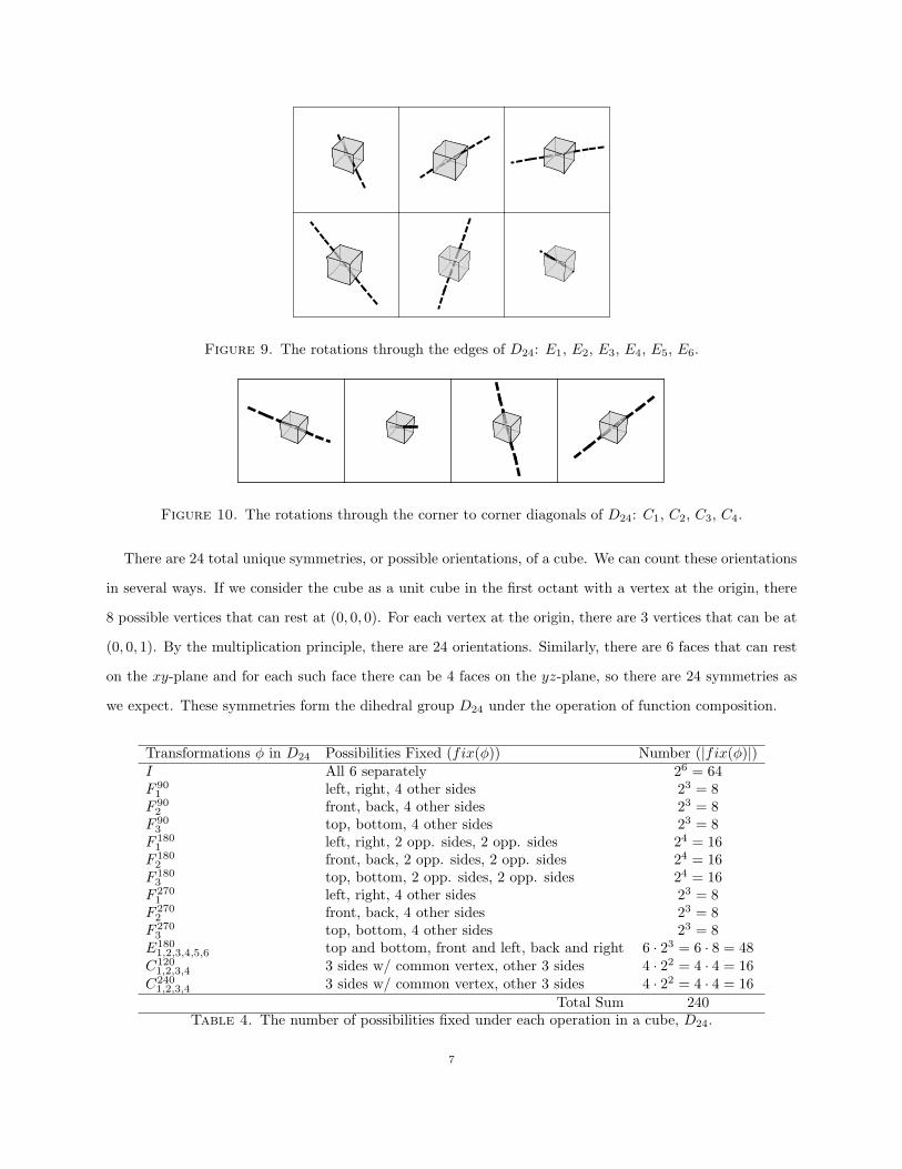
Figure 9. The rotations through the edges of D24: E1, E2, E3, E4, E5, E6.

Figure 10. The rotations through the corner to corner diagonals of D24: C1, C2, C3, C4.

There are 24 total unique symmetries, or possible orientations, of a cube. We can count these orientations

in several ways. If we consider the cube as a unit cube in the first octant with a vertex at the origin, there

8 possible vertices that can rest at (0, 0, 0). For each vertex at the origin, there are 3 vertices that can be at

(0, 0, 1). By the multiplication principle, there are 24 orientations. Similarly, there are 6 faces that can rest

on the xy-plane and for each such face there can be 4 faces on the yz-plane, so there are 24 symmetries as

we expect. These symmetries form the dihedral group D24 under the operation of function composition.

Transformations φ in D24 Possibilities Fixed (fix(φ)) Number (|fix(φ)|)I All 6 separately 26 = 64F 90

1 left, right, 4 other sides 23 = 8F 90

2 front, back, 4 other sides 23 = 8F 90

3 top, bottom, 4 other sides 23 = 8F 180

1 left, right, 2 opp. sides, 2 opp. sides 24 = 16F 180

2 front, back, 2 opp. sides, 2 opp. sides 24 = 16F 180

3 top, bottom, 2 opp. sides, 2 opp. sides 24 = 16F 270

1 left, right, 4 other sides 23 = 8F 270

2 front, back, 4 other sides 23 = 8F 270

3 top, bottom, 4 other sides 23 = 8E180

1,2,3,4,5,6 top and bottom, front and left, back and right 6 · 23 = 6 · 8 = 48C120

1,2,3,4 3 sides w/ common vertex, other 3 sides 4 · 22 = 4 · 4 = 16C240

1,2,3,4 3 sides w/ common vertex, other 3 sides 4 · 22 = 4 · 4 = 16Total Sum 240

Table 4. The number of possibilities fixed under each operation in a cube, D24.

7

Next, we will examine the number of sides fixed by each transformation. These are detailed in Table 4.

We can see that for a cube, the sum over all elements of D24 of the number of possible colorings fixed by

each transformation is equal to the size of D24 times the number of varieties. In this case, 240 = 24 · 10.

From this data and that from the 6-beaded necklace, we claim that the number of varieties is equal to the

order of the dihedral group times the total number of choices of sets of sides fixed by each transformation.

2.4. The Proof of Burnside’s Theorem. Now, we prove our conjecture after introducing more math.

Definition 2.4. (Equivalence Relation [3]) An equivalence relation on a set S is a set R of ordered pairs of

elements of S such that

(1) (a, a) ∈ R for all a ∈ S (reflexive property)

(2) (a, b) ∈ R implies (b, a) ∈ R (symmetric property)

(3) (a, b) ∈ R and (b, c) ∈ R imply (a, c) ∈ R (transitive property)

Definition 2.5. (Partition [3]) A partition of a set S is a collection of nonempty disjoint subsets of S whose

union is S.

Theorem 2.1. (Equivalence Classes Partition [3]) The equivalence classes of an equivalence relation on a

set S constitute a partition of S. Conversely, for any partition P of S, there is an equivalence relation on S

whose equivalence classes are the elements of P .

Definition 2.6. (Subgroup [3]) If a subset H of a group G is itself a group under the operation of G, we

say that H is a subgroup of G, denoted H ≤ G.

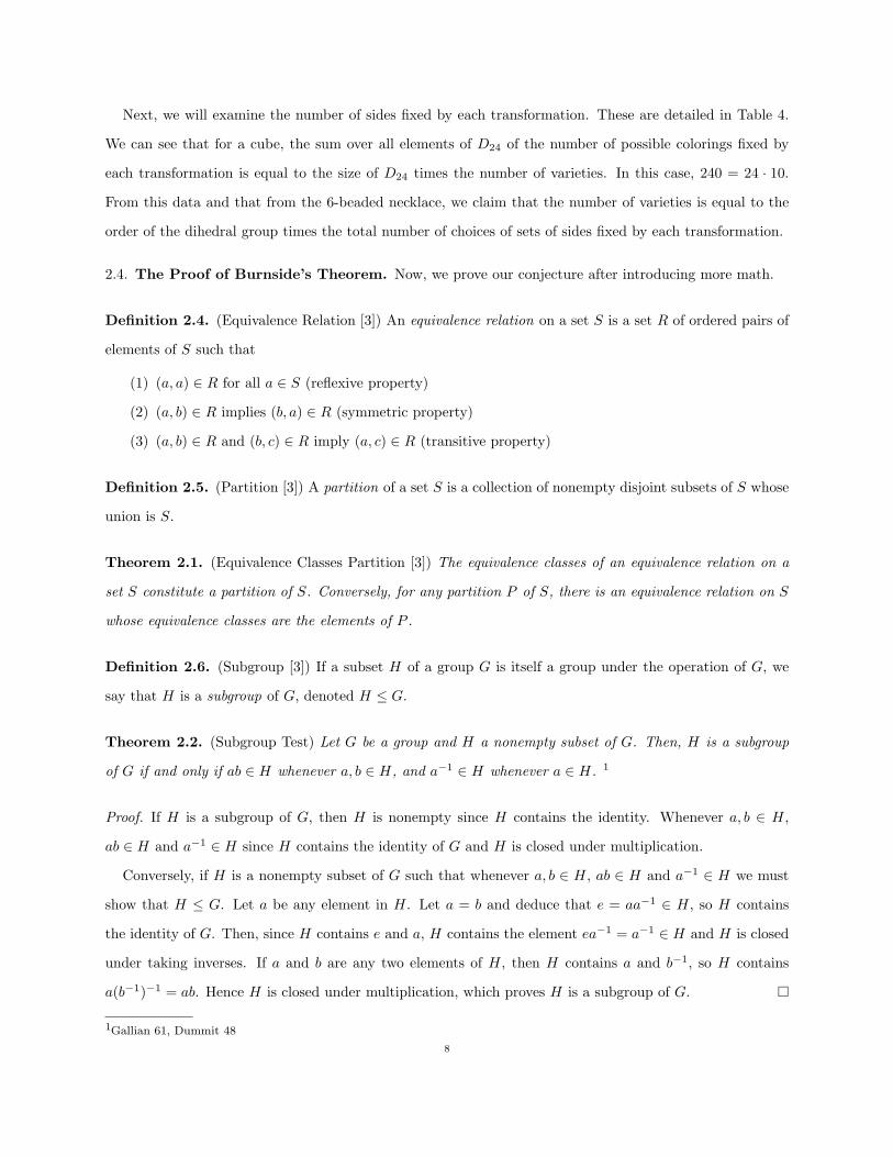
Theorem 2.2. (Subgroup Test) Let G be a group and H a nonempty subset of G. Then, H is a subgroup

of G if and only if ab ∈ H whenever a, b ∈ H, and a−1 ∈ H whenever a ∈ H. 1

Proof. If H is a subgroup of G, then H is nonempty since H contains the identity. Whenever a, b ∈ H,

ab ∈ H and a−1 ∈ H since H contains the identity of G and H is closed under multiplication.

Conversely, if H is a nonempty subset of G such that whenever a, b ∈ H, ab ∈ H and a−1 ∈ H we must

show that H ≤ G. Let a be any element in H. Let a = b and deduce that e = aa−1 ∈ H, so H contains

the identity of G. Then, since H contains e and a, H contains the element ea−1 = a−1 ∈ H and H is closed

under taking inverses. If a and b are any two elements of H, then H contains a and b−1, so H contains

a(b−1)−1 = ab. Hence H is closed under multiplication, which proves H is a subgroup of G. �

1Gallian 61, Dummit 48

8

Example 2.2. Consider the group Z4 = {0, 1, 2, 3} and its subset {0, 2}. We will show that {0, 2} ≤ Z4

using Theorem 2.2. First, we check for closure under addition: 0 + 0 = 0, 0 + 2 = 2, and 2 + 2 = 0. Next, we

check for closure under taking inverses: 0−1 = 0 and 2−1 = 2. Therefore {0, 2} is indeed a subgroup of Z4.

Definition 2.7. (Coset of H in G [3]) Let G be a group and H a subgroup of G. For any a ∈ G, the set

{ah such that h ∈ H}, denoted by aH, is called the left coset of H in G containing a.

Lemma 2.2.1. (Properties of Cosets [3]) Let H be a subgroup of G, and let a and b belong to G. Then,

(1) a ∈ aH,

(2) aH = H if and only if a ∈ H,

(3) aH = bH or aH ∩ bH = ∅,

(4) aH = bH if and only if a−1b ∈ H,

(5) |aH| = |bH| if H is finite,

(6) aH = Ha if and only if H = aHa−1,

(7) aH is a subgroup of G if and only if a ∈ H.

Theorem 2.3. (Lagrange’s Theorem [3]) If G is a finite group and H is a subgroup of G, then |H| divides

|G|. Moreover, the number of distince left (right) cosets of H in G is |G||H| .

Proof. Let a1H, a2H, ..., arH denote the distinct left cosets of H in G. Then, for each a ∈ G, we have

aH = aiH for some i. By property 1 of cosets, a ∈ aH. Thus, each member of G belongs to one of the

cosets aiH. In symbols, G = a1H ∪ ...∪ arH. Now, property 3 of cosets shows that this union is disjoint, so

|G| = |a1H|+ |a2H|+ ...+ |arH|. Finally, since |aiH| = |H| for each i, we have |G| = r|H|. �

Definition 2.8. (Permutation of a Set S [3]) A permutation of a set S is a function from S to S that is

both one-to-one and onto.

Definition 2.9. (Permutation Group of S [3]) A permutation group of a set S is a set of permutations of

S that forms a group under function composition.

Definition 2.10. (Stabilizer of a Point [3]) Let G be a group of permutations of a set S. For each s ∈ S,

let stabG(s) = {g ∈ G such that g(s) = s}. We call stabG(s) the stabilizer of s ∈ G.

Example 2.3. The stabilizer of the cube in Figure 2.4 consists of I, F 901 , F 180

1 , and F 2701 . These are the

rotations about the vertical line of symmetry through the middle of the top and bottom faces.9

Figure 11. Stabilizer Example

Definition 2.11. (Orbit of a Point [3]) Let G be a group of permutations of a set S. For each s ∈ S, set

orbG(s) = {g(s) such that g ∈ G}. The set orbG(s) is a subset of S called the orbit of s under G.

Figure 12. Orbit Example

Example 2.4. The orbit of the cube in Figure 2.4 consists of all orientations of a cube with one light side.

Definition 2.12. (Elements Fixed by g [3]) For any group G of permutations on a set S and any g ∈ G,

we let fix(g) = {s ∈ S such that g(s) = s}. This set is called the fix of g.

Figure 13. Fix Example

Example 2.5. The cubes fixed under C1, corner-corner diagonal symmetry are pictured in Figure 2.4.10

Lemma 2.3.1. ( Stabilizer is a Subgroup [3]) The stabilizer of s in G is a subgroup of G.

Proof. Let s ∈ S and define stabG(s) = {g ∈ G such that g(s) = s}. The identity element of G, e, is in

stabG(s) since e(s) = s. Let g1, g2 ∈ stabG(s). Then

g1 ◦ g2(s) = g1(g2(s)) = g1(s) = s

and stabG(s) is closed under function composition.

Let g ∈ stabG(s) and consider g−1. Given that e(s) = s,

g−1 ◦ g(s) = g−1(s) = e(s) = s = g(s) = g ◦ g−1(s)

so stabG(s) is closed under inverses. �

Lemma 2.3.2. ( Orbits Partition [3]) Given that G is a group of permutations of a set S, the orbits of the

members of S constitute a partition of S.

Proof. To prove that the orbits of the members of S constitute a partition of S, we must show that the

orbits are equivalence classes of the set S. Let s1, s2, s3 ∈ S and g1, g2, g3 ∈ G. Certainly, s1 ∈ orbG(s1).

Now suppose s3 ∈ orbG(s1) ∩ orbG(s2). Then s3 = g1(s1) and s3 = g2(s2), and therefore (g−12 (g1(s1)) = s2.

So, if s3 ∈ orbG(s2), then s3 = g3(s2) = (g3(g−12 (g1(s1))) for some g3. This proves orbG(s2) ⊆ orbG(s1). By

symmetry, orbG(s1) ⊆ orbG(s2). �

Theorem 2.4. (Orbit-Stabilizer Theorem [3]) Let G be a finite group of permutations of a set S. Then, for

any s ∈ S, |G| = |orbG(s)| · |stabG(s)|.

Proof. By Lagrange’s Theorem (Theorem 2.3), |G||stabG(s)| is the number of distinct left (right) cosets of

stabG(s) in G. Thus, it suffices to establish a one-to-one correspondence between the left cosets of stabG(s)

and the elements in the orbit of s. To do this, we define a correspondence T by mapping the coset g1 ·stabG(s)

to g1(s) under T . To show that T is a well-defined function, we must show that g1 · stabG(s) = g2 · stabG(s)

implies that g1(s) = g2(s). But g1 · stabG(s) = g2 · stabG(s) implies g−11 g2 ∈ stabG(s), so that (g−1

1 g2)(s) = s

and, therefore, g2(i) = g1(i). Reversing the argument from the last step to the first step shows that T is also

one-to-one. We conclude the proof by showing that T is onto orbG(s). Let s2 ∈ orbG(s1). Then g1(s1) = s2

for some g1 ∈ G and T (g1 · stabG(s1)) = g1(s1) = s2, so T is onto. �

11

applying the permutation g ∈ G is orbG(s). The fix(g) is the set of colorings in S that are invariant under

g ∈ G. According to Burnside’s theorem (Theorem 2.5), The number of orbits of G on S, or the number of

colorings distinct under G is124

∑g∈G|fix(g)|.

The values for |fix(g)| can be found in Table 4, so∑g∈G|fix(g)| = 240. The result is that there are 10 distinct

orbits, or varieties, for a two-colored cube.

2.5. Tetrahedron. Burnside’s theorem does not place a restriction on the number of color choices. For

example, examine a tetrahedron colored with k colors using Burnside’s theorem (Theorem 2.5). A tetrahedron

has four faces so our set S = {bottom, left, right, front} and |S| = 4. Let their be k possible colors for each

face. Therefore, we count k4 possible colorings for an immobile tetrahedron. A tetrahedron has 12 different

symmetries, so |G| = 12 and the group G contains the following transformations.

• I

The first is the identity operation, or any rotation of zero degrees.

• V 1201,2,3,4, V 240

1,2,3,4

Next are rotations of 120 and 240 degrees about the 4 lines of symmetry from each vertex to the

center of the opposite side.

• E1801,2,3

Finally, there are rotations of 180 degrees about the three lines of symmetry that go from the center

of one edge to the center of the center of the opposite edge.

The fix(g) for each g ∈ G are represented in Table 5. Substituting these numbers into Theorem 2.5, we get

112· (k4 + 11k2) = (number of distinct k-colored tetrahedrons under G).

If we substitute in k = 2 to calculate the number of 2-colored tetrahedrons, we get

112· (24 + 11 · 22) =

112· 60 = 5.

We can verify that there are indeed five varieties of two-colored tetrahedrons by observation.

3. Polya’s Theorem

3.1. Motivation. In the cube counting problem (Example 2.7), Burnside’s theorem (Theorem 2.5) allows

us to calculate the number of varieties of two-colored cubes under the group D24, but it does not tell us

much about those varieties. Let the colors of the cube be denoted L for the light colored faces and D for13

g fix(g) |fix(g)|I All 4 separately k4

V 1201,2,3,4 bottom, other three sides 4 · k2

V 2401,2,3,4 bottom, other three sides 4 · k2

E1801,2,3 top and left, bottom and right 3 · k2

Total Sum k4 + 11k2

Table 5. The number of possible colorings fixed under each symmetry of a k-colored tetrahedron.

the dark colored faces. We generate a polynomial for some g ∈ G such that each grouping of sides in fix(g)

is represented by the factor (La +Da) where a is the number of sides in the grouping.

For example, the identity element of G is represented by the polynomial (L + D)6 since each face can

be colored separately and remain invariant under I for each of the 6 sides that complete our cube. Next,

consider F 1803 . In this case, the top of the cube can be any color, the bottom can be any color, the front and

back must be the same color, and the left and right sides must be the same color. The top and the bottom

are both represented by (L+D). The set containing the front and back is represented by (L2 +D2). We take

the product of all four terms, so our polynomial representing F 1803 is (L+D)2(L2 +D2)2. The polynomials

for the other terms are represented in Table 6.

If we take the sum of all of the polynomials (each polynomial represents an element of G) for a two-colored

cube, we get

(2) 24(L6 + L5D + 2L4D2 + 2L3D3 + 2L2D4 + LD5 +D6).

Notice that in Equation 2 that after factoring out |G| (24 in this case), the coefficients of the terms are

informative. The coefficient of LD5 = 1 and there is exactly 1 variety with 1 light side and 5 dark sides. The

coefficient of L3D3 = 2 and there are exactly two varieties of cubes with 3 light sides and 3 dark sides. We

did not start with any more information than we did for Burnside’s theorem (Theorem 2.5), but we learn

more about the colorings using polynomials.

φ ∈ D24 Polynomial ExpansionI (L+D)6 L6 + 6L5D + 15L4D2 + 20L3D3 + 15L2D4 + 6LD5 +D6

F 901,2,3 3 · (L+D)2(L4 +W 4) 3 · (L6 + 2L5D + L4D2 + L2D4 + 2LD5 +D6)F 180

1,2,3 3 · (L+D)2(L2 +D2)2 3 · (L6 + 2L5D + 3L4D2 + 4L3D3 + 3L2D4 + 2LD5 +D6)F 270

1,2,3 3 · (L+D)2(L4 +W 4) 3 · (L6 + 2L5D + L4D2 + L2D4 + 2LD5 +D6)E180

1,2,3,4,5,6 6 · (L2 +D2)3 6 · (L6 + 3L4D2 + 3L2D4 +D6)C120

1,2,3,4 4 · (L3 +D3)2 4 · (L6 + 2L3D3 +D6)C240

1,2,3,4 4 · (L3 +D3)2 4 · (L6 + 2L3D3 +D6)Sum 24(L6 + L5D + 2L4D2 + 2L3D3 + 2L2D4 + LD5 +D6)

Table 6. The polynomials for each symmetry of a 2-colored cube in D24.

14

3.2. Cycle Index of a Permutation Group. We begin our build up to Polya’s theorem with more

discussion of permutations. The cycle index of a permutation group is a polynomial used in Polya’s theorem

and many of its extensions.

Theorem 3.1. ( Products of Disjoint Cycles [3]) Every permutation of a finite set can be written as a cycle

or as a product of disjoint cycles.

Proof. Let S be a finite set where |S| = m and let g be a permutation of S. To write g in disjoint cycle form,

choose any s1 ∈ S and let s2 = g(s1), s3 = g(g(s1)) = g2(s1), ... until s1 = πl(s1) for some l. We know

that such an l exists because the sequence must be finite. Say gi(s1) = gj(s1) for some i and j with i < j.

Then s1 = gl(s1), where l = j − i. We express this relationship among s1, s2, ..., sl as g = (s1, s2, ..., sl)....

It is possible that we have not exhausted the set S in this process. So, we pick any t1 ∈ S not appearing

in the first cycle and generate a new cycle. That is, we let t2 = g(t1) and so on until we reach t1 = gk(t1)

for some k. This new cycle has no elements in common with the previously constructed cycle. For, if it did,

then gi(s1) = gj(t1) for some i and j. But then, gi−j(s1) = t1, and therefore t1 = sr for some r. This is a

contradiction since t1 is not contained in cycle s. Continuing this process until we run out of elements of S,

our permutation will appear as g = (s1, s2, ..., sl)(t1, ..., tk)...(c1, ..., cr). In this way, every permutation

can be written as a product of disjoint cycles. �

If g is a permutation of a finite set S, we can split S into disjoint cycles, or subsets of S cyclically permuted

by g. Given a cycle of length l, the elements of the cycle are s, g(s), g2(s), ..., gl−1(s).

Definition 3.1. (Type [2]) If permutation g splits S into b1 cycles of length 1, b2 cycles of length 2, etc., g

is of type {b1, b2, b3, ... }.

We can see that bi = 0 for i > |S|. Also, bi = 0 for all but at most a finite number of i’s. Also,

|S| = b1 + 2b2 + 3b3+....

Definition 3.2. (Cycle Index [2]) If G is a permutation group, for each g ∈ G, consider the product

x1b1x2

b2 · · ·xmbm where g is of type {b1, b2, ...}. The cycle index of G is the polynomial

(3) PG(x1, x2, ..., xm) =1|G|

∑g∈G

x1b1x2

b2 · · ·xmbm

Example 3.1. Let G = {e}, or the identity permutation of S. We can see that e is of type {m, 0, 0, ...}

since it has m cycles of length 1, so its cycle index is equal to xm1 .15

Example 3.2. Let G be the permutation group generated by (123)(456)(78). The each element of group G

is of type {0, 1, 2} and therefore

PG(x1, x2, x3) =16

∑g∈G

x2x23 = x2x

23.

Example 3.3. [2]Let S be the set of cube faces and G be the permutation group of S. Using our previously

defined notation and descriptions of the symmetries of a cube, we can visualize

• I is of type {6, 0, 0, ...}.

• F 1801,2,3 are of type {2, 2, 0, 0, ...}.

• F 90,2701,2,3 are of type {2, 0, 0, 1, 0, ...}.

• E1801,2,3,4,5,6 are of type {0, 3, 0, 0, ...}.

• V 120,2401,2,3,4 are of type {0, 0, 2, 0, 0, ...}.

Since |G| = 24 and 1 + 3 + 6 + 6 + 8 = 24, our list of symmetries is exhaustive. We calculate the cycle index

of G to be

(4) PG =124

(x61 + 3x2

1x22 + 6x2

1x4 + 6x32 + 8x2

3).

The following theorems and definitions help us understand the next example: the cycle index of the Cayley

representation of a general finite set.

Definition 3.3. (Group Isomorphism) An isomorphism φ from a group G to a group G is a one-to-one and

onto mapping from G to G that preserves the group operation. That is,

(5) φ(g1g2) = φ(g1)φ(g2) for all g1, g2 ∈ G.

Theorem 3.2. (Cayley’s Theorem [3]) Every group is isomorphic to a group of permutations.

Proof. Let G be any group. We will find a group G of permutations that is isomorphic to G. For any g ∈ G,

define function Tg : G 7→ G by Tg(x) = gx for all x ∈ G. To prove that Tg is a permutation on the set of

elements in G, we show that Tg : G 7→ G is one-to-one and onto. For all g ∈ G, Tg(x) = gx ∈ G by the

group property of closure. Given gx1 = gx2, by cancellation x1 = x2, and thus Tg is one-to-one. Given any

x1 ∈ G, there exists an x2 ∈ G such that Tg(x2) = gx2 = x1 thus Tg is onto.

For the permutation Tg, we show that that if g runs through G, then the Tg’s form a permutation group

G of G. First, G is nonempty since if e is the identity of G. For all x ∈ G, x = ex = ge(x) ∈ G. For all

g1, g2, g3 ∈ G, G is associative since (Tg1Tg2)Tg3(x) = (g1g2)g3x = g1(g2g3)(x) = Tg1(Tg2Tg3)x. Next we16

show that G is closed under multiplication and taking inverses. If g1 and g2 are in group G, g1g2 is also in

G. From the way we defined Tg, we see that Tg1Tg2(x) = g1g2x = Tg1g2(x) ∈ G. The inverse of Tg = gx is

T−1g (x) = g−1x since TgT−1

g (x) = gg−1x = ex = x for all x ∈ G and therefore all Tg ∈ G. By Theorem 2.2,

G is a group.

For every g ∈ G, define φ(g) = Tg. If Tg = Th, then Tg(e) = Th(e) or ge = he. Thus, g = h and φ is

one-to-one. By the way G is constructed, φ is onto. For some g1, g2 ∈ G, φ(g1g2) = Tg1Tg2 = φ(g1)φ(g2).

Therefore φ is an isomorphism from G to G. G is called the Cayley representation of the group G. �

Example 3.4. [2]Let S be any finite group, and let |S| = m. If s is a fixed element of S, then for all x ∈ S,

the mapping S 7→ sx is a permutation of S. Denoting this permutation gs, if s runs through S, the gs’s

form a permutation group G. By Cayley’s Theorem and its proof, G is isomorphic to S and is the Cayley

representation of S. We are interested in its cycle index.

If s ∈ S, let the order of s be |s| = k(s). Permutation gs splits S into cycles of length k(s), since if

s ∈ S, the cycle obtained by gs is {x, sx, s2x, ..., sk(s)x = x}. These cycles are cosets of S. It follows from

Lagrange’s Theorem (Theorem 2.3) that for each k(s) | m and there are mk(s) cycles of length k(s). Thus,

the cycle index of G is

(6) PG =1m

∑s∈S

[xk(s)]m

k(s) .

3.3. Weighted Form of Burnside’s Theorem. Earlier, we discussed Burnside’s theorem in which the

elements ofG are permutations. It is a trivial extension so say that now the elements ofG act as permutations.

That is, to each g ∈ G we have attached a permutation of S denoted πg. The mapping is homomorphic, or

πgg′ = πgπg′ for all g, g′ ∈ G. We say that two elements of S are equivalent, or s1 ∼ s2, if there exists a

g ∈ G such that πgs1 = s2. The equivalent classes of S are called transitive sets. We now state our weighted

form of Burnside’s theorem.

Theorem 3.3. (Weighted Burnside’s Theorem [2]) Given set S, group G, and permutation group πG, the

number of transitive sets equals

(7)1|G|

∑g∈G

ψ(g),

where |G| denotes the number of elements of G, and for each g ∈ G, ψ(g) denotes the number of elements

of S that are invariant under πg.17

This is the weighted version of Burnside’s theorem since the different elements of G need not correspond

to different permutations π. Since we are adding up all of the πg’s, some may be counted more than once.

3.4. Functions and Patterns. Let D, domain, and R, range, be finite sets. Let the set of all functions

from D into R be denoted RD, where the number of elements in RD is |R||D| since for each d ∈ D, we have

|R| choices for f(d). Let G be a permutation group of D.

Definition 3.4. (Pattern [2]) Given f1, f2 ∈ RD, we call f1 and f2 equivalent, or f1 ∼ f2 if there exists a

g ∈ G such that f1(gd) = f2(d) for all d ∈ D. These equivalence classes are called patterns.

We confirm that f1g = f2 is indeed an equivalence relation. The relation is reflexive because f ∼ f by

the identity permutation in G. The relation is symmetric since f1 ∼ f2 then f2 ∼ f1 since if g ∈ G implies

g−1 ∈ G. The relation is transitive since if f1 ∼ f2 and f2 ∼ f3, then f1 ∼ f3 because G is closed under

multiplication.

Example 3.5. [2]Let D be the set of six faces of a cube. Let G be the group of permutations of D by

symmetry. Let R be the colors light and dark. The set of all possible colorings of a fixed cube is RD and the

number of colorings is |R||D| = 26. The number of varieties of rotatable cubes, also called transitive sets,

orbits of G, or patterns, is 10. The method for arriving at these numbers has been explained in Example

2.7.

Example 3.6. [2]Let D = {1, 2, 3}, let G be the symmetric group of D (the group of all permutation), and

let R = {x, y}. We can see that there are eight functions, but only four patterns as shown in Table 7. Since

Pattern Corresponding Functionsx3 f(1) = f(2) = f(3) = xx2y f(1) = f(2) = x, f(3) = y; f(1) = f(3) = x, f(2) = y; f(2) = f(3) = x, f(1) = yy2x f(1) = f(2) = y, f(3) = x; f(1) = f(3) = y, f(2) = x; f(2) = f(3) = y, f(1) = xy3 f(1) = f(2) = f(3) = y

Table 7. The functions and patterns when D = {1, 2, 3}, R = {x, y}, and G = S3.

the symmetric group does not depend on the order of the factors, functions f1 and f2 are equivalent if and

only if the products f1(1)f1(2)f1(3) and f2(1)f2(2)f2(3) are identical.

We have stated the weighted version of Burnside’s theorem. Now, we define the weights.

3.5. Weights of Functions and Patterns.

Definition 3.5. (Ring [3]) A ring R is a nonempty set with two binary operations, addition and

multiplication, such that for all a, b, c ∈ R:18

(1) a+ b = b+ a.

(2) (a+ b) + c = a+ (b+ c).

(3) There is an additive identity 0. That is, there is an element 0 in R such that a+ 0 = a for all a ∈ R.

(4) There is an element −a ∈ R such that a+ (−a) = 0.

(5) a(bc) = (ab)c.

(6) a(b+ c) = ab+ ac and (b+ c)a = ba+ bc.

A ring is called a commutative ring if ab = ba for all a, b ∈ R.

Definition 3.6. (Weight [2]) Given that D and R are finite sets, the set of all functions from D into R

is RD, and G is a permutation group of D. We assign each element in R a weight. This weight can be a

number, a variable, or generally, an element of a commutative ring containing the rational numbers. The

weight for each r ∈ R is denoted w(r).

Definition 3.7. (Weight of a Function [2]) The weight of a function f ∈ RD, denoted W(f) is

(8) W (f) =∏d∈D

w[f(d)].

If f1 ∼ f2, or the functions belong to the same pattern, then they have the same weight. This is because

if f1g = f2 for all g ∈ G. Using the fact that the same factors are involved and they are commutative we

conclude that ∏d∈D

w[f1(d)] =∏d∈D

w[f1(g(d))] =∏d∈D

w[f2(d)].

Definition 3.8. (Weight of a Pattern [2]) The weight of a pattern F , denoted W (F ), is equal to the weight

of any (and every) function in F . Given any f ∈ F ,

(9) W (F ) =∏d∈D

w[f(d)].

Example 3.7. [2]Recall the light gray and dark gray cube from Example 3.5. Let D be the set of faces,

R = {light, dark}, and let G be is the set of symmetries. We set weights, w(light) = x and w(dark) = y,

the weights for each of the 10 patterns are: x6, x5y, x4y2, x3y3, x3, y3, x2y4, xy5, y6. Different patterns need

not have different weights. For example, x3y3 represents the pattern with three light sides and three dark

sides in two ways: three dark sides meet at a single corner, three dark sides that wrap around the cube.

Example 3.8. [2]Recall Example 3.6 where D = {1, 2, 3}, G is the symmetric group of D, and R = {x, y}.

We set w(x) = x and w(y) = y so x3, x2y, xy2, and y3 become the pattern weights. In this case, different19

Figure 14. Two cubes with the same weight and different patterns.

patterns have different weights. If we set w(r) = 1 for all r ∈ R, then W (f) = 1 for all f ∈ F , and therefore

W (F ) = 1 for each pattern.

3.6. Store and Inventory.

Definition 3.9. (Store [2]) Given that D and R are finite sets and every r ∈ R has a weight w(r), the set

of all functions from D into R is RD, and G is a permutation group of D. We call R the store because it is

the set from which we choose function values.

Definition 3.10. (Inventory [2]) Since the values of w(r) must come from a commutative ring, the weights

can be added to each other. The store enumerator, or inventory of R is

(10) inventory of R =∑r∈R

w(r).

Example 3.9. Let us say that a cafe owner has 3 candy bars that cost $1 each, 2 bottles of pop that cost

$3 each, and 4 hamburgers in stock that cost $5 each. His store is R = {c1, c2, c3, p1, p2, h1, h2, h3, h4}.

Depending on the values to which we set the weights, the inventory of R will give us different information:

• To get complete information about the store, we can set the weight values at w(c1) = c1, w(c2) =

c2, ..., w(h4) = h4. Then the inventory of R = c1 + c2 + c3 + p1 + p2 + h1 + h2 + h3 + h4.

• We might only be interested in the number of items of each type. In this case, we set the weights as

w(c1) = w(c2) = w(c3) = c and w(p1) = w(p2) = p and w(h1) = w(h2) = w(h3) = w(h4) = h. In

this case, the inventory of R = 3c+ 2p+ 4h.

• To get the value of the store, we set the weights as w(c1) = w(c2) = w(c3) = 1 and w(p1) = w(p2) = 3

and w(h1) = w(h2) = w(h3) = w(h4) = 5. In this case, the inventory of R = 3 ·1 + 2 ·3 + 4 ·5 = $29.

• To get the number of items in the store, we set the weights as w(c1) = 1, w(c2) = 1, ..., w(h4) = 1.

Then the inventory of R = 1 + 1 + 1 + 1 + 1 + 1 + 1 + 1 + 1 = 9.20

3.7. Inventory of a Function. We are given that D and R are finite sets, every r ∈ R has a weight w(r),

the set of all functions from D into R is RD, every function f ∈ RD has weight

w(f) =∏d∈D

w[f(d)],

and G is a permutation group of D. The inventory of RD is the |D|th power of the inventory of R:

(11) inventory of RD =∏f

W (f) =

[∑r∈R

w(r)

]|D|.

We can write the |D|th power of∑r∈R

w(r) as the product of the |D| factors. In each factor

∑r∈R

w(r),

pick a term w(r). By taking the product of these terms, we get one term of the full expansion. Since each

factor has |R| terms, there are |R||D| terms in the full expansion. Next, we take f(d) = r which allows us

to say that the selection of a term from a factor is a one-to-one mapping f of D into R. To every f there

corresponds the term

(12)∏d∈D

w[f(d)]

of the full expansion. Since the term in (12) is exactly the definition of W (f) in (8), or the weight of a

function, the full product is equal to the sum of all W (f), which is the inventory of |R||D|.

[2]Next, we will derive the inventory of S, a certain subset of |R||D|. First, partition D into k disjoint

components D1, D2, ...Dk such that |D| = |D1|+ |D2|+ ...+ |Dk|. Let S be the set of all functions f that are

constant on each component. They may, but do not have to be different on different components. Let f be

expressed as a composition of two functions, φ and ψ, such that f = φψ. The function ψ maps d onto the

index of the component to which d belongs, so we always have d ∈ Dψ(d). The function φ is the mapping

from {1, 2, ..., k} into R, so there are |R|k possibilities for φ. Therefore,

(13) inventory of S =k∏i=1

∑r∈R

[w(r)]|Di|.

We can see this same result for the inventory of S by examining the full expansion of the product. To select

one term of the product, we pick a value for φ which is a mapping from {1, 2, ..., k} into R. This φ produces

21

the term

{w[φ(1)]}|D1| · {w[φ(2)]}|D2| · · · {w[φ(k)]}|Dk| =k∏i=1

{w[φ(i)]}|Di|.

If φψ = f , then this term is exactly W (f) since

{w[φ(i)]}|Di| =∏d∈Di

w{φ[ψ(d)]},

andk∏i=1

∏d∈Di

w[f(d)] = W (f).

In this way, each f ∈ S is obtained exactly once. Thus the sum of W (f) for all f ∈ S is equal to the sum of

all terms of the expansion of the inventory of S.

Example 3.10. [2]Given m identical counters, we pass them out between three people, P1, P2, P3, under

the constraint that you give the same number to P1 and P2. How many ways are there to do this?

Let D = {P1, P2, P3}, R = {0, 1, 2, ...}, f(P1) = f(P2), and f(P1) + f(P2) + f(P3) = m. First we separate

D into D1 = {P1, P2} and D2 = {P3}. Then we set the weights of R such that 0, 1, 2, 3, ... have weights

1, x, x2, x3, ... and the weight of the functions W (f) = xm. If S is the set of all functions constant on each

Di, and by (13), the inventory of the set of all functions constant on each Di equals

(14) (1 + x2 + x4 + · · · )(1 + x+ x2 + · · · ).

We are seeking the coefficient of xm in the expansion (14). Using the formula for the sum of a geometric

series,1

1− x=∞∑i=0

xi,

we can simplify our inventory to1

1− x2· 1

1− x.

Then we expand this result using partial fractions to

11− x2

· 11− x

=A

1 + x+

B

(1− x)2+

C

1− x

=A(1− x)2(1− x) +B(1 + x)(1− x) + C(1 + x)(1− x)2

(1 + x)(1− x)2(1− x)22

Next, substitute, A = 14 , B = 1

2 , and C = 14 to get

14 (1− x)2(1− x)

(1 + x)(1− x)2(1− x)+

12 (1 + x)(1− x)

(1 + x)(1− x)2(1− x)+

12 (1 + x)(1− x)2

(1 + x)(1− x)2(1− x)

=14

(1 + x)−1 +12

(1− x)−2 +14

(1− x)−1.

For the number of possible distributions we obtain

(15)12

(m+ 1) +14

[1 + (−1)m]

so the number of function is 12m+ 1 if m is even and 1

2m+ 12 if m is odd.

Let [xk] denote the coefficient of the xk-term. We will verify (15) result directly for small values of m:

• If m = 1, the inventory is (1 + x2)(1 + x), and the x-term is 1 · x so [x] = 1. In words, there is 1

possibility for the distribution of 1 counter and that is 0 to P1 and P2 and 1 to P3.

• If m = 2, the inventory is (1 + x2 + x4)(1 + x+ x2), and the x2-term is 1 · x2 + x2 · 1 so [x2] = 2. In

words, there are 2 possibilities for the distribution of 2 counters and those are: 1 each to P1 and P2

and 0 to P3; 0 to P1 and P2 and 2 to P3.

• If m = 3, the inventory is (1 + x2 + x4 + x6)(1 + x + x2 + x3), and the x3-term is 1 · x3 + x2 · x so

[x3] = 2. In words, there are 2 possibilities for the distribution of 3 counters: 1 each to P1, P2, and

P3; 0 to P1 and P2 and 3 to P3.

• If m = 4, the inventory is (1 + x2 + x4 + x6 + x8)(1 + x + x2 + x3 + x4), and the x4-term is

1 · x4 + x2 · x2 + x4 · 1 so [x4] = 3. The possibilities for the distribution of 4 counters are: 2 each to

P1 and P2 and 0 to P3; 1 each to P1 and P2 and 2 to P3; 0 each to P1 and P2 and 4 to P3.

These results are concur with (15) and also give us more information on the possible distributions.

3.8. The Pattern Inventory.

Theorem 3.4. (Polya’s Fundamental Theorem [2]) We are given finite sets D and R, a permutation group

G of D, each r ∈ R has weight w(r), each function f ∈ RD and the patterns F have weights W (f) and

W (F ). The pattern inventory is

(16)∑F

W (F ) = PG

{∑r∈R

w(r),∑r∈R

[w(r)]2,∑r∈R

[w(r)]3, ...

}

where PG is the cycle index of G.

Proof. Let R and D be finite sets, RD be the set of all functions from D into R, and G a permutation group

of D. Let S be the subset of function f ∈ RD such that W (f(d)) = w. If g ∈ G, and f1(d) = f2(gd), then f1

23

and f2 belong to the same pattern and have the same weight. Therefore, if f1 ∈ S, then f1g−1 ∈ S. Thus

for each g ∈ G there is a mapping πg of S into itself,

πg(f(d)) = f(g−1d).

This mapping is a permutation since (πg)−1 = πg(−1) . For each f ∈ S, if g, g′ ∈ G, for all d ∈ D,

πgg′(f(d)) = f((gg′)−1d) = f(g′−1g−1d) = πg(f(g′−1d)) = πg(πg′f(d))

and the mapping g → πg is homomorphic.

We say the f1 and f2 are equivalent if and only if

f1(d) = f2(g−1d) = πg(f2(d)).

Therefore, the patterns contained in S are equivalence classes. According to the weighted Burnside’s theorem,

the number of patterns contained in S is equal to

1|G|

∑g∈G

ψw(g),

where ψw(g) is the number of functions f such that W (f) = w. This is equivalent to f(g−1(d)) = f(d) =

πg(f(d)) or f(d) = f(g(d)).

The patterns contained in S all have weight w; therefore if we multiply (7), the weighted Burnside theorem,

by w and sum over all possible values of w, we obtain the pattern inventory

∑W (F ) =

1|G|

∑w

∑g∈G

w · ψw(g).

We have ∑w

w · ψw(g) =(g)∑f

W (f),

where(g)∑f

means the summation over all f ∈ RD that satisfies f(d) = f(gd) for all d ∈ D. It follows that

∑W (F ) =

1|G|

∑g∈G

(g)∑f

W (f).

24

In order to evaluate(g)∑f

W (f), we remark that g is a permutation of D, and therefore splits D into cycles

that are cyclically permuted by g. The condition f(d) = f(gd) means that

f(d) = f(gd) = f(g2d) = · · · ,

where f is constant on each cycle of D. Conversely, each f that is constant on every cycle automatically

satisfies f(gd) = f(d) since g(d) always belongs to the same cycle as d itself. Thus if the cycles are

D1, D2, ..., Dk, then the sum(g)∑f

is just the inventory of S from (13).

Let {b1, b2, ...} be the type of g. This means, among the numbers |D1|, ..., |Dk|, the number 1 occurs b1

times, the number 2 occurs b2 times, etc. Consequently, we have

(g)∑f

=

{∑r∈R

w(r)

}b1·

{∑r∈R

[w(r)]2}b2· · · .

The number of factors in finite, but we need not invent a notation for the last one since all bi are zero from

a certain i onward. The expression above can be obtained by the substitution of

x1 =∑r∈R

w(r), x2 =∑r∈R

[w(r)]2, x3 =∑

r ∈ R[w(r)]3,...

into the product xb11 xb22 x

b33 · · · , which is the term corresponding for g in |G| ·PG. Summing with respect to g

and dividing by |G|, we infer that the value of the pattern index,∑W (F ), is obtained by making the same

substitution into PG(x1, x2, x3, ...), and this proves Polya’s theorem. �

Example 3.11. If all of the weights are chosen to be equal to unity, then we obtain that the number of

patterns is equal to Pg(|R|, |R|, |R|, ...). We can show this by directly substituting w(r) = 1 for all r ∈ R.

The pattern inventory becomes simply the number of pattern which is equal to PG(|R|, |R|, |R|, ...).

Example 3.12. Consider the light and dark painted cube. Let D bet he set of faces of the cube, G be the

set of rotational symmetries, R be the set of colors, {light, dark}.

Let the weights w(light) = 1 and w(dark) = 1. Then from Example 3.11,

the number of patterns = PG(|R|, |R|, |R|, ..)

and we obtain124

(26 + 3 · 24 + 6 · 23 + 6 · 23 + 8 · 22) = 10.

This is the same number of patterns that we discovered by inspection and then derived by Burnside’s theorem.25

Example 3.13. [2]Now, let the weights w(light) = x and w(dark) = y. First, calculate the pattern

inventory using Polya’s theorem,

∑F

W (F ) = PG

{∑r∈R

w(r),∑r∈R

[w(r)]2,∑r∈R

[w(r)]3, ...

}.

Recall the the cycle index of G is

PG(x1, x2, x3, x4) =124

(x61 + 3x2

1x22 + 6x2

1x4 + 6x32 + 8x2

3).

Next, the we substitute∑r∈R

[w(r)]i for the xi’s. Therefore, the pattern inventory is

124

[(x+ y)6 + 3(x+ y)2(x2 + y2)2 + 6(x+ y)2(x4 + y4) + 6(x2 + y2)3+8(x3 + y3)2].

Expanding the pattern inventory, we get

124

(x6 + x5y + 2x3y3 + 2x2y4 + xy5 + y6).

This polynomial can be interpreted to give us complete information about the possible colorings of the cube.

For example, we might ask how many patterns have four light faces and two dark faces. The answer is the

coefficient of the x4y2-term, [x4y2] = 2. This is consistent with the value that we found in (2). Also, the

sum of the coefficients is predictably equal to ten, which is the total number of patterns.

Example 3.14. [2]Let D be a finite set, and let G be a permutation group of D. We call two subsets of D,

D1 and D2, equivalent if for some g ∈ G, we have gD1 = D2. In other words, D2 is the set of all elements

gd obtained by letting d run through D1. We can form classes of equivalent subsets in this manner.

We can create functions, fg(d) = gd, that are in one-to-one correspondence with the subsets. Let R =

{light, dark}, w(light) = 1, and w(dark) = 1. In this case, the number of subset classes is equal to the

pattern inventory, which by Polya’s theorem, is equal to PG(2, 2, 2, ...).

Now let w(light) = w and w(dark) = 1, where w is a variable. Then the subsets of k elements correspond

to functions f with W (f) = wk. Therefore, the number of equivalence classes which consist of subsets of k

elements is equal to the coefficient of wk in the pattern inventory, PG(1 + w, 1 + w2, 1 + w3, ..). Summing

over all k, we obtain PG(2, 2, 2, ...) since the sum of the coefficients of a polynomial p(w) is equal to p(1).

This example relates strongly to the cube problem. For example, let a subset D be equal to the set of all

cubes with just one side light. There exists some g ∈ G such that all cubes with one light side are equivalent

to all of the other cubes with one light side, but not to any cubes with a different number of light sides.26

Then the cycle index is the same as it is for any two colored cube. The pattern inventory is now

124

[(w + 1)6 + 3(w + 1)2(w2 + 1)2 + 6(w + 1)2(w4 + 1) + 6(w2 + 1)3 + 8(w3 + 1)2].

If we expand the pattern inventory, we get

w6 + w5 + 2w3 + 2w2 + w + 1.

We can create the same two colored cubes as before using these simplified calculations simply by painting

the complementary faces dark.

4. Generalizations and Extensions of Polya’s Theorem

4.1. Generalization of Polya’s Theorem. In Polya’s theorem, G, a permutation group of D induced

an equivalence relation on the mappings f ∈ RD. Now, we consider a second permutation group H of R

with a new equivalence relation on the mappings f ∈ RD which is defined based on both groups. Let f1 be

equivalent to f2 if there exists a g ∈ G, h ∈ H such that f1g = hf2. We now show that

(17) f1g = hf2 or f1(g(d)) = h(f2(d)) for all d ∈ D

is an equivalence relation.

(1) If g and h are identity permutations, f1(g(d)) = h(f1(d)) so f1 ∼ f1 and (17) satisfies the reflexive

property.

(2) If f1 ∼ f2, there exists a g ∈ G, h ∈ H such that f1(g(d)) = h(f2(d)) for all d ∈ D. Since g−1(d) ∈ D

since G is a permutation group, f1(g(g−1(d))) = h(f2(g−1(d)), so f2(g−1(d)) = h−1(f1(d)) for all d

in D so f2 ∼ f1. Therefore (17) satisfies the symmetric property.

(3) If f1 ∼ f2 and f2 ∼ f3, then there exists g, g′ ∈ G, h, h′ ∈ H such that f1(g(d)) = h(f2(d′)) and

f2(g′(d)) = h′(f3(d)). Let d′ = g′(d). Then f1(g(g′(d)) = h(f2(g′(d))) = h(h′(f3(d))) since g, g′ ∈ G

and h, h′ ∈ H. Therefore f1 ∼ f3 and (17) satisfies the transitive property.

Therefore (17) is an equivalence relation so RD splits into equivalence classes, or patterns.

We assume that each f ∈ RD has a weight W (f) such that the the weights are elements of a commutative

ring. We need not assume that the W (f) are obtained from the elements of R, but we do assume that

equivalent functions have the same weight, or

(18) f1 ∼ f2 =⇒ W (f1) = W (f2).27

If F is a pattern, we define its weights W (F ) to be the common value of all W (f) with f ∈ F just as we did

for Polya’s theorem (Theorem 3.4). As our first extension of Polya’s theorem, we now calculate the pattern

inventory, or the sum of the weights of all patterns, using equivalence relation (17).

Theorem 4.1. (de Bruijn’s Extension [2]) Given finite sets, D and R, functions f ∈ RD, and permutation

groups G on D and H on R, the pattern inventory is

(19)∑

W (F ) =1

|G| · |H|∑g∈G

∑h∈H

(g,h)∑f

W (f)

where(g,h)∑f

is the sum of W (f) extended over all f that satisfy fg = hf .

Example 4.1. Consider a 6-beaded necklace. You care about the pattern, but not the colors of the beads.

For example, you are color blind, and able to distinguish between colors but not identify them. In math

terminology, the colors are ”unlabelled.” In this case, D is the let of beads, R is the set of colors {light, dark},

G = D6, and H = S2. We set all of the weights equal to w(light) = 1 and w(dark) = 1. By Theorem 4.1,

the pattern inventory is

∑W (F ) =

1|G| · |H|

∑g∈G

∑h∈H

(g,h)∑f

W (f) =1

24 · 2· 288 = 6

The 6 cubes are: all one color, 5 sides one color, and 4 sides on color in two ways.

4.2. The Kranz Group. Let S and T be finite sets with G and H as permutation groups of finite sets S

and T . Consider S ⊕ T . Choose a g ∈ G and for each s ∈ S, pick an hs ∈ H. These elements determine a

permutation of S ⊕ T .

(s, t)→ (g(s), hs(t)) such that s ∈ S, t ∈ T

There are |G| · |H||S| permutations of the form (s, t) → (g(s), hs(t)) such that s ∈ S and t ∈ T . These

permutations form a group called the Kranz group G[H]. We will now calculate the cycle-index of this group.

Theorem 4.2. ( Polya’s Kranz Theorem [2]) The cycle-index of G[H], is

PG[H](x1, x2, x3, ...) = PG[PH(x1, x2, ...), PH(x2, x4, ...), ...]

where the right hand side is obtained by substituting

yk = PH(xk, x2k, x3k, ...)28

into

PG(y1, y2, y3, ...).

Proof. Given a finite set R such that each r ∈ R has weight w(r), consider mappings from T into R. These

mappings form patterns λ and the equivalence classes induced by H, a permutation group of R. Let Λ be

the set of these patterns. That pattern inventory is

∑λ∈Λ

W (λ) = PH

{∑w(r),

∑[w(r)]2, ...

}.

Now, consider mappings of S into Λ that form patterns ψ by means of the equivalence relation defined by

G, a permutation group of S. After defining weights W ∗(ψ), we obtain the inventory of the ψ’s

∑ψ

PG

{W (λ),

∑[W (λ)]2,

∑[W (λ)]3, ...

}.

The sums∑

[W (λ)]2, etc. are obtained by applying the pattern inventory of Λ to new weights, w2, w3, ....

Therefore, our pattern inventory of the ψ’s equals the expression that we obtain by substituting

x1 =∑

w(r), x2 =∑

[w(r)]2, ...

into the right hand side of

PG[H](x1, x2, x3, ...) = PG[PH(x1, x2, ...), PH(x2, x4, ...), ...].

After that, we construct a one-to-one correspondence between the set of ψ’s and the patterns that arise from

the equivalence introduced by G[H] in the set R(S⊕T ). We can also substitute for the w(r)’s in the inventory

of Λ. Finally, we get our equation since R and w are arbitrary. �

Example 4.2. [2]Given n cubes whose faces are light or dark. How many ways can we color the cubes

when the equivalence classes are defined by permutations of the set of cubes and rotations of the separate

cubes?

The Kranz group under consideration is Sn[G], where Sn is the symmetric group of degree n and G is

the dihedral group of the rotations of the cube. To calculate the number of patterns, we substitute x1 =

x2 = ... = 2 into the cycle index. Making this substitution into any of PG(x1, x2, x3, ...), PG(x2, x4, x6, ...),

and PG(x3, x6, x9, ...), we always get PG(2, 2, 2, ...), and this is equal to 10 which is the number of varieties

of cubes. Thus, the answer to our question is Sn(10, 10, 10, ...). This is the coefficient of wn in the Taylor29

expansion of

exp(10w +12· 10w2 +

13· 10w3 + · · · ) = (1− w)−10,

and therefore

Sn(10, 10, 10, ...) =(n+ 9)!n!9!

.

Example 4.3. [2]How many of the preceding patterns have the property that they do not change if we

interchange the colors?

This number if found by substituting

x1 = x3 = x5 = · · · = 0, x2 = x4 = x6 = · · · = 2

into the cycle index. The polynomials become PG(0, 2, 0, 2, ...) and PG(2, 2, 2, ...), alternately. As

PG(0, 2, 0, 2...) = 2 we obtain

PSn[G](0, 2, 0, 2, ...) = PSn(2, 10, 2, 10, ...).

This is the coefficient of wn in

exp(2w +12· 10w2 +

13· 2w3 + ...)

which simplifies to

1 + 2w + 7w2 + 12w3 + 27w4 + 42w5 + 77w6 + ...

so our answer for n = 5 is 42 patterns.

5. Applications to Graph Theory

5.1. Superposition Theorem. [4]Polya’s theorem and its extensions are related to the superposition

theorem. We uses the superposition theorem to solve the same problem as Example 4.1.

We are given an ordered set of k permutation groups of degree n: G1, G2, ..., Gk. The set of all k-ads

(a1, a2, ..., ak) where ai ∈ Gi. Two k-ads (a1, a2, ..., ak) and (b1, b2, ..., bk) are similar if there exists an x ∈ Sn

and gi ∈ Gi such that bi = xaigi for i = 1, ..., k. The superposition theorem gives us a method for calculating

the number of equivalence classes.

For a graphical interpretation of this principle, let Ti where i = 1, ..., k be a set of k graphs with p

vertices. Let Gi be the automorphism group of Ti, or the graphs obtained by superposing k graphs on the

same vertices. We distinguish the edges by coloring the edges of each graph different colors. The isomorphism30

classes of the superimposed graphs are the equivalence classes for G1, G2, ..., Gk. The superposition principle

give us the number of nonisomorphic superimposed graphs.

We can compute the cycle index of Gi to be

Z(Gi) =1|Gi|

∑(j)

A(i)(j)s

j11 s

j22 · · · sjpp

where A(i)(j) is the number of permutations of cycle type (j) = (j1, j2, ..., jp) in Ti. So the number of equivalent

classes is ∏(i)

1|Gi|

∑(j)

A1(j)A

2(j) · · ·A

k(j)(1

j1j1! · 2j2j2! · · · pjpjp!)k−1

This is more easily seen by defining function ? such that if

A =∑(j)

a(j)sj11 s

j22 · · · sjpp

and

B =∑(j)

b(j)sj11 s

j22 · · · sjpp

then

A ? B =∑(j)

a(j)b(j)∏(i)

(ij1j1!)sj11 sj22 · · · sjpp

such that for each monomial sj11 sj22 · · · s

jpp the coefficient in A ? B is the product of the coefficient of that

monomial in A and B times 1j1j1! · · · pjpjp!. So, if A And B are the cycle indices of two graphs, A?B is the

sum of the cycle indices of the automorphism groups of the distinct superimposed graphs.

If C is an expression in s1, s2, ..., sp, define N(C) to be the result of setting s1 = s2 = ...sp = 1. For each

cycle index A, if N(A) = 1, then N(A ? B) is equal to the number of superpositions of two graphs. Also,

A?B can be extended to any number of superpositions. If Ai is the cycle index of the automorphism group

of Ti, the product of Z(Gi), then the number of superposed graphs is N(A1 ? A2 ? ... ? Ak) which we write

as N(G1 ? G2 ? ... ? Gk).

Example 5.1. [4]Consider the six- beaded necklace. Let D be the 6 beads. Let R be the colors light

and dark. Let G = D6 and let H = S2 (interchanges the elements of R). We want to find the number of

distinct configurations of two light beads and four dark beads. Let w(light) = x and w(dark) = y. Therefore

the inventory of R is x + y. We can use Polya’s theorem to derive the pattern inventory PD6(x + y). The

number of necklaces with two light beads and four dark beads is the coefficient of the monomial x2y4 in the

expansion of the pattern inventory.31

To solve this using the superposition theorem, consider the graphs in Figure 15. The superposition of the

two graphs have a one-to-one correspondence with the necklaces. The number of necklaces can be seen as

N(D6 ? (S2 ⊕ S4)) since the direct product S2 ⊕ S4 is the group automorphism of Figure 16. Since

PD6 =112

(x61 + 2x6 + 2x2

3 + 4x32 + 3x2

1x22)

and

PS2⊕S4 =148

(x61 + 7x4

1x2 + 9x21x

22 + 8x3

1x3 + 6x21x3 + 3x2

2 + 8x1x2x3 + 6x2x4)

we have

N(D6 ? (S2 ⊕ S4)) =1

12 · 48(6! + 4 · 3 · 3! · 23 + 3 · 9 · 2 · 22 · 2) = 3.

We can see that this is the correct answer by calculating out the entire polynomial using Polya’s theorem

(as in Example 4.1) and by direct observation of the possible arrangements of two light beads and four dark

beads as in the introduction to this paper. This is exactly the coefficient of the x2y4 term in the pattern

index of a 2-color 6-beaded necklace.

Figure 15. The two superimposed graphs in Example 5.1.

Figure 16. The automorphism graph in Example 5.1.

5.2. Another Generalization. The next important generalization of Polya’s theorem was published in

1966 by Harary and Palmer [4]. We are given D, R, f : D → R ∈ RD and perform permutations G on D

and H on R with the equivalence relations defined as in de Bruijn’s generalization. We create a group of

permutations of the functions induced by G and H. Given the each function f is in the power set RD, we

now have the power group HG and we then compute the cycle index of this group.32

If the look at the necklace problem again, with D as the six beads, R as the colors light and dark, H

interchanges the colors and G permutes the beads. The total number of possibilities (can use unweighted

function) is1|H|

∑h∈H

PG(c1(h), ..., cm(h))

such that

ck(h) =∑α|k

αjα(h).

Let G = D6 and H = S2. These permutations are of type x21 and x2 respectively. Therefore x2

1 corresponds

to ck(h) = xjx = 2 for all k and x1 corresponds to ck(h) = 2 if k is even. Therefore the configuration

generating function is12PD6(2, 2, 2, ...) + PD6(0, 2, 0, 2, ...) = 8.

We can compare this to PD6(2, 2, 2, ...) = 13 when the colors are not interchangeable. This means that there

are three necklaces that are now equivalent to themselves when we are able to interchange the colors as in

Example 4.1. This happens to be the value of PD6(0, 2, 0, 2...).

6. Conclusion

In this paper, we begin by counting the number of colored shapes under the dihedral groups. First, we

count a cube and hexagon by observation. Then we use algebra to derive Burnside’s theorem and Polya’s

theorem. Finally, we note some generalizations of Polya’s theorem which are related to our original counting

problems.

A major application of Polya’s theorem which we do not cover is the enumeration of graphs and trees.

Some further reading on Polya’s theorem and its generalizations and applications are the works of Frank

Harary, N.G. de Bruijn, and Polya’s original paper. De Bruijn published a paper after the one used as a

source in this paper which further generalizes Polya’s theorem. Harary has several papers which include

extensions of Polya’s main theorem and applications to graph theory. Polya’s original paper focusses on the

applications to chemical enumeration. [4]

References

[1] Brualdi, Richard A., Introductory Combinatorics, 5th Edition. New Jersey: Pearson Education, 2010.

[2] De Bruijn, N.G., ”Polya’s Theory of Counting.” In Applied Combinatorial Mathematics, edited by Beckenbach, Edwin F.

New York: J. Wiley, 1964.

[3] Gallian, Joseph A., Contemporary Abstract Algebra, 5th Edition. Massachusetts: Houghton Mifflin Company, 2002.

33

[4] Read, Ronald C., ”The Legacy of Polya’s Paper: Fifty Years of Polya Theory.” In Combinatorial Enumeration of Groups,

Graphs, and Chemical Compounds. New York: Springer-Verlag, 1987.

34

enumeration by algebraic combinatorics 1. introduction

Documents