enumerating graph embeddings and partial-duals by genus

numerativeombinatorics

pplications

A Enumerative Combinatorics and Applicationsecajournal.haifa.ac.il

ECA 1:1 (2021) Article #S2S1https://doi.org/10.54550/ECA2021V1S1S1

Enumerating Graph Embeddings and Partial-Duals by Genus and Euler Genus

Jonathan L. Gross† and Thomas W. Tucker‡

†Department of Computer Science, Columbia University, New York, NY 10027 USAEmail: [email protected]

‡Department of Mathematics, Colgate University, Hamilton, NY 13346, USAEmail: [email protected]

Received: September 2, 2020, Accepted: November 16, 2020, Published: November 20, 2020

The authors: Released under the CC BY-ND license (International 4.0)

Abstract: We present an overview of an enumerative approach to topological graph theory, involving the

derivation of generating functions for a set of graph embeddings, according to the topological types of their

respective surfaces. We are mainly concerned with methods for calculating two kinds of polynomials:

1. the genus polynomial ΓG(z) for a given graph G, which is taken over all orientable embeddings of G, and

the Euler-genus polynomial EG(z), which is taken over all embeddings;

2. the partial-duality polynomials ∂E∗G(z), ∂E

×G(z), and ∂E

∗×∗G (z), which are taken over the partial-duals for

all subsets of edges, for Poincare duality (∗), Petrie duality (×), and Wilson duality (∗×∗), respectively.

We describe the methods used for the computation of recursions and closed formulas for genus polynomials

and partial-dual polynomials. We also describe methods used to examine the polynomials pertaining to some

special families of graphs or graph embeddings, for the possible properties of interpolation and log-concavity.

Mathematics Subject Classifications: 05A05; 05A15; 05C10; 05C30; 05C31

Key words and phrases: Genus polynomial; Graph embedding; Log-concavity; Partial duality; Production

matrix; Ribbon graph; Monodromy

1. Introduction

We are concerned with two classes of enumerative invariants regarding the embeddings of graphs in surfacesof arbitrarily high genus or crosscap number. One class is the embedding polynomials of a graph, as initiatedby [24]. The other is the partial-duality polynomials of a graph embedding, which are recently introducedinvariants [30–32], in which the authors have taken a special interest.

In this overview, we encounter three different paradigms for specifying a graph embedding.

1. Rotation systems — the dominant paradigm for combinatorial specification of embeddings; introduced byHeffter [41] and Edmonds [17].

2. Ribbon graphs — used by Chmutov [16] to give a geometric definition of partial Poincare duals.

3. Monodromy — the dominant paradigm in algebraic map theory; introduced by Jones and Singerman [43]

In general, we allow a graph to have loops and multi-edges. Each edge is construed to have two half-edges(that meet midway along the length of the edge). We label the edges of a graph by the integers 1, 2, . . . , n, andwe denote the half-edges of edge j by j+ and j−. A direction of traversal of an edge may be given by specifyingthe half-edge that is traversed first. A graph is taken to be connected, unless it is evident from context thatwe mean otherwise. The genus of an orientable surface is denoted by γ(S). The orientable surface of genus j

†Jonathan Gross is supported by Simons Foundation Grant No. 315001‡Thomas Tucker is supported by Simons Foundation Grant No. 317689

Jonathan L. Gross and Thomas W. Tucker

is denoted Sj and the non-orientable surface of crosscap-number k is denoted Nk. Some prior familiarity withtopological graph theory beyond planarity is assumed. Some recommended sources are [37] or [64].

Section 2 describes the paradigm of rotation systems. Section 3 presents methods used in their derivations forthe genus polynomials of what are called linear sequences and ring-like sequences of graphs. Section 4 describesmethods for other kinds of graphs, including some important non-linear families for which family-wide genuspolynomial formulas are known. Section 5 discusses some possible structural attributes of these embedding-related polynomials, especially log-concavity. Section 6 describes the paradigms of monodromy and ribbongraphs. Section 7 discusses all three kinds of duals of graph embeddings and their corresponding partial duals.Section 8 presents formulas for the partial-dual polynomials of several sequences of ribbon graphs. Section 9suggests a number of problems for investigation.

We have italics on various technical terms to indicate that their definitions appear later, usually along withsome developmental detail.

2. Rotation systems

A rotation at a vertex v of an oriented embedding of a graph G is a cyclic list of the half-edges incident at v,in the order consistent with the orientation of the surface. The collection of rotations, one at every vertex, iscalled a rotation system for G, commonly denoted by ρ. It has long been known that the oriented embeddingsof a graph G are in bijective correspondence with the set of all possible rotation systems for G. This has thefollowing immediate implication:

Proposition 2.1. The total number of oriented embeddings of a graph G equals∏v∈V (G)

(δ(v)− 1)! (1)

where V (G) is the vertex set of G and δ(v) is its valence (or degree).

When we compose a rotation system ρ for an embedded graph with the full involution (commonly denoted byλ) that reverses the directions of the edges, the result is a permutation whose cycles correspond to the boundarywalks for the faces of the embedding. Thus, the embedding could be reconstructed by fitting a polygon to eachof those cycles and pasting the polygons together.

Proposition 2.2. The face-boundary walks of an embedding with rotation system ρ are given by the compo-sition ρλ. (The composition ρλ means λ is applied first.)

Given an embedding (called the primal embedding) of a graph in a surface, we form a Poincare dual of Gand its embedding as follows:

1. place a dual vertex in the interior of each region of the primal embedding;

2. through each primal edge e (i.e., of the graph G), draw a dual edge e∗ that joins the dual vertex on oneside of e to the dual vertex on its other side. If a single face of the primal embedding is incident on bothsides of edge e, then the dual edge e∗ is a loop.

According to [1], knowledge of the duality between the cube and the octahedron, and between the dodecahedronand the icosahedron goes back to the “fifteenth book of Euclid”, which [1] estimates as having originated inthe sixth century C.E. Poincare developed algebraic consequences of a generalization of this topological form ofduality to higher dimensions.

Corollary 2.1. The rotation system for the Poincare dual of an embedding with rotation system ρ is given bythe composition ρλ.

The minimum genus of a graph G, denoted γmin

(G) is the smallest genus of a surface in which G can beembedded. The maximum genus, denoted γmax(G) is the largest genus of a surface in which G can be cellularlyembedded , which means embedded so that the interior of every region is homeomorphic to an open disk. Thegenus polynomial of the graph G, as defined by [24], is the formula

ΓG(z) =

γmax (G)∑j=γ

min(G)

gj(G)zj , (2)

where gj(G) is the number of embeddings of G in the orientable surface Sj . Two analogous polynomials havebeen defined subsequently [7]:

1. the crosscap-number polynomial XG(z), which enumerates embeddings of G in non-orientable surfaces Nj ,according to crosscap number j; and

2. the Euler-genus polynomial EG(z), which enumerates embeddings of G in all surfaces, according to Eulergenus.

ECA 1:1 (2021) Article #S2S1 2


3. Genus polynomial formulas for linear graph families

This section begins with a description of methods that have been used for derivation of formulas for the genusof graphs that are grouped into a linear sequence. We follow this with discussion of ring-like sequences, in whicheach graph is obtained by some kind of self-amalgamation of a graph in a corresponding linear sequence.

Two embeddings of a graph G are topologically equivalent if one can be obtained from the other by ambientisotopy. When a graph is embedded in a surface, the induced rotation at a vertex means the cyclic ordering ofhalf-edges that are encountered as we traverse a small circle surrounding the vertex. If the surface is oriented,then we traverse each such circle in the direction consistent with the orientation. Then the induced rotationsystem is the set of such vertex rotations. It has long been known that two embeddings of a graph aretopologically equivalent if and only if their induced rotation systems are the same.

If the embedding surface is non-orientable, then we choose a spanning tree T , and then choose the vertexrotations so that any two vertex rotations are consistent whenever the two vertices are endpoints of the sametree edge. A co-tree edge in either embedding of G is said to be twisted whenever the rotations at its endpointsare inconsistent. Then two embeddings are topologically equivalent if and only if they have not only the samerotation systems but also the same sets of twisted edges, relative to a spanning tree T . See [37] for furtherdetails.

3.1 Linear sequences of graphs

A linear sequence of graphs is a sequence constructed recursively, as now introduced via an example. By aladder graph (or simply ladder), we mean the cartesian product graph of a path graph with the complete graphK2. The genus polynomials of ladder graphs were derived by [19]. Figure 1 illustrates the ladder sequence andthe ingredients of their recursive construction.

. . .

L0 L1 L2 H

(a) (b)

Figure 1: (a) Sequence of ladder graphs. (b) Subgraph for the recursion.

The base graph for a recursive construction is the ladder L0, a vertical copy of K2. We construct the ladderLn by amalgamating the two vertices at the left end of the subgraph H to the two endpoints of the rightmostrung of the ladder Ln−1.

According to Formula (1), the ladder Ln has 2n−2 embeddings. In order to construct their genus polynomials,the key step is partitioning the embeddings into two types. An embedding of type d has two different face-boundary walks incident on its rightmost edge. An embedding of type s has the same face-boundary walktwice incident on that edge. We define the numbers dj(Ln) and sj(Ln) to be the numbers of type-d and type-sembeddings of Ln, of genus j, respectively, which leads to the type-d and type-s partial genus polynomials

DLn(z) =

n∑j=0

dj(Ln)zj (3)

SLn(z) =

n∑j=0

sj(Ln)zj . (4)

Figure 2 illustrates the four ways that subgraph H can be added to a ladder of type-d or of type-s. We seek toconvert such a figure into a simultaneous recursion.

H(s)

Ln

Ln

H(d)

Figure 2: (d) Adding H to a type-d ladder. (s) Adding H to a type-s ladder.



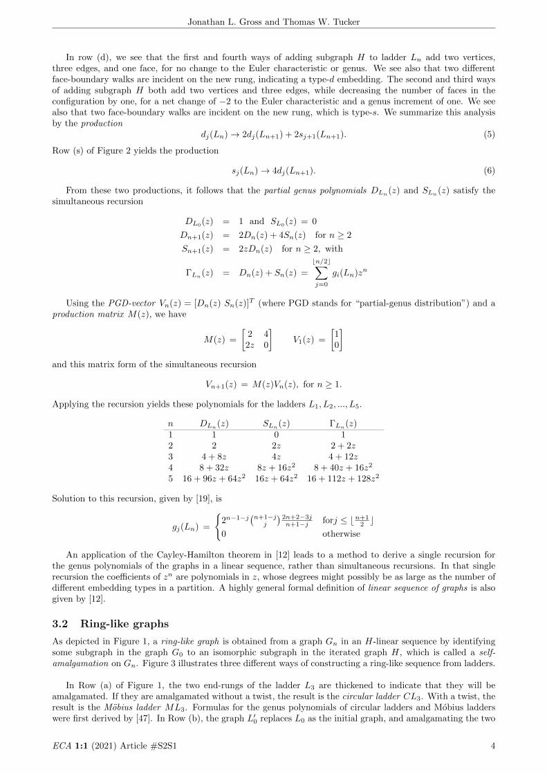
In row (d), we see that the first and fourth ways of adding subgraph H to ladder Ln add two vertices,three edges, and one face, for no change to the Euler characteristic or genus. We see also that two differentface-boundary walks are incident on the new rung, indicating a type-d embedding. The second and third waysof adding subgraph H both add two vertices and three edges, while decreasing the number of faces in theconfiguration by one, for a net change of −2 to the Euler characteristic and a genus increment of one. We seealso that two face-boundary walks are incident on the new rung, which is type-s. We summarize this analysisby the production

dj(Ln)→ 2dj(Ln+1) + 2sj+1(Ln+1). (5)

Row (s) of Figure 2 yields the production

sj(Ln)→ 4dj(Ln+1). (6)

From these two productions, it follows that the partial genus polynomials DLn(z) and SLn(z) satisfy thesimultaneous recursion

DL0(z) = 1 and SL0(z) = 0

Dn+1(z) = 2Dn(z) + 4Sn(z) for n ≥ 2

Sn+1(z) = 2zDn(z) for n ≥ 2, with

ΓLn(z) = Dn(z) + Sn(z) =

bn/2c∑j=0

gi(Ln)zn

Using the PGD-vector Vn(z) = [Dn(z) Sn(z)]T (where PGD stands for “partial-genus distribution”) and aproduction matrix M(z), we have

M(z) =

[2 42z 0

]V1(z) =

[10

]and this matrix form of the simultaneous recursion

Vn+1(z) = M(z)Vn(z), for n ≥ 1.

Applying the recursion yields these polynomials for the ladders L1, L2, ..., L5.

n DLn(z) SLn

(z) ΓLn(z)

1 1 0 12 2 2z 2 + 2z3 4 + 8z 4z 4 + 12z4 8 + 32z 8z + 16z2 8 + 40z + 16z2

5 16 + 96z + 64z2 16z + 64z2 16 + 112z + 128z2

Solution to this recursion, given by [19], is

gj(Ln) =

{2n−1−j

(n+1−j

j

)2n+2−3jn+1−j forj ≤ bn+1

2 c0 otherwise

An application of the Cayley-Hamilton theorem in [12] leads to a method to derive a single recursion forthe genus polynomials of the graphs in a linear sequence, rather than simultaneous recursions. In that singlerecursion the coefficients of zn are polynomials in z, whose degrees might possibly be as large as the number ofdifferent embedding types in a partition. A highly general formal definition of linear sequence of graphs is alsogiven by [12].

3.2 Ring-like graphs

As depicted in Figure 1, a ring-like graph is obtained from a graph Gn in an H-linear sequence by identifyingsome subgraph in the graph G0 to an isomorphic subgraph in the iterated graph H, which is called a self-amalgamation on Gn. Figure 3 illustrates three different ways of constructing a ring-like sequence from ladders.

In Row (a) of Figure 1, the two end-rungs of the ladder L3 are thickened to indicate that they will beamalgamated. If they are amalgamated without a twist, the result is the circular ladder CL3. With a twist, theresult is the Mobius ladder ML3. Formulas for the genus polynomials of circular ladders and Mobius ladderswere first derived by [47]. In Row (b), the graph L′0 replaces L0 as the initial graph, and amalgamating the two



L0 L3

CL3

H

L'0 L'3H

(a)

(b)

ML3

RL4

Figure 3: The circular ladder CL3, the Mobius ladder ML3, and the Ringel ladder RL4 as ring-like con-structions.

thickened subgraphs in L′3 yields the Ringel ladder RL4. The graphs RLn were introduced by Gustin [38] ascurrent graphs and used to spectacular advantage by Ringel and Youngs [55] in their solution to the Heawoodmap-coloring problem. A formula for the genus polynomials of Ringel ladders was derived by [60].

The effects of the topological operation of self-amalgamating a graph G on a single vertex and on a singleedge on the genus polynomial of G are derived by [20] and [52], respectively. A more general study of the effectson genus polynomials and crosscap polynomials of the conversion from linear sequences to ring-like sequencesis given by [7].

We recall (e.g., [56]) that Chebyshev polynomials of the second kind are defined, for n ≥ 0, by the formula

Un(cos θ) =sin(n+ 1)θ

sin θ.

Equivalently, Un(x) is a polynomial of degree n in z with integer coefficients, given by the recurrence

U0(z) = 1,

U1(z) = 2z, and

Un(z) = 2zUn−1(z)− Un−2(z).

We further recall that the generating function for the Chebyshev polynomials is given by∑n≥0

Un(z)tn =1

1− 2zt+ t2. (7)

Using Chebyshev polynomials, the genus polynomials of Ringel ladders and of circular ladders were rederivedby [34] and [10], respectively, and the log-concavity of the polynomials in both sequences was established.

The non-orientable embedding distributions for ladders and a couple of other sequences of graphs werederived by [5] by using the rank of the overlap matrix of [48]. Non-orientable embedding distributions forRingel ladders were obtained by [15].

4. Non-linear families

There are two kinds of non-linear families of graphs whose genus polynomials are known. In a family of thefirst kind, the graphs typically have only one or two vertices of increasing valence. A member graph of four ofthese families is shown in Figure 4. Discussion of families of the second kind appears in §4.2.

bouquet B3 dipole D4 wheel W6fan F5

Figure 4: A bouquet, a dipole, a fan, and a wheel.

4.1 One or two vertices of high valence

The genus polynomials for several families of graphs with only one or two vertices of increasing valence havebeen calculated by counting the number of certain kinds of permutations with a given number of cycles. Wedenote the symmetric group on m symbols by Σm. We denote the number of cycles of a permutation π by |π|.



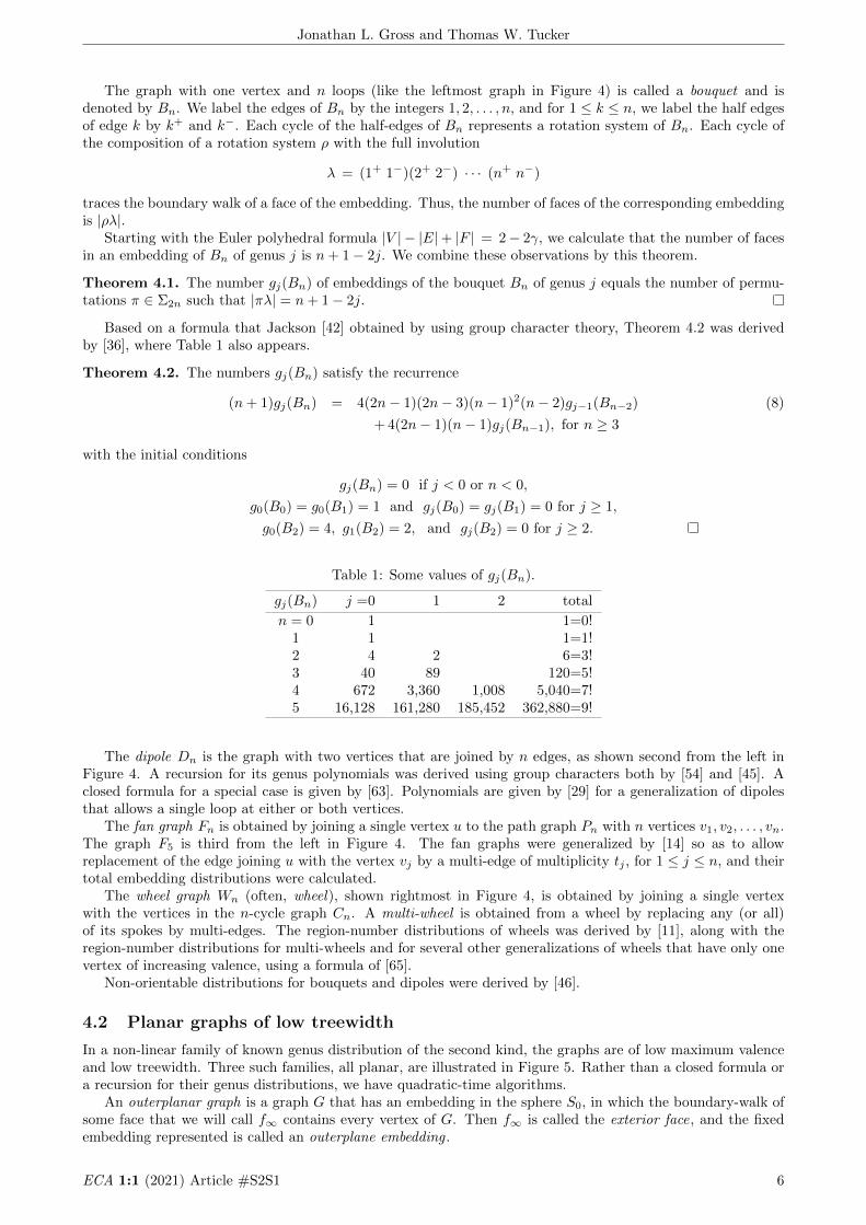
The graph with one vertex and n loops (like the leftmost graph in Figure 4) is called a bouquet and isdenoted by Bn. We label the edges of Bn by the integers 1, 2, . . . , n, and for 1 ≤ k ≤ n, we label the half edgesof edge k by k+ and k−. Each cycle of the half-edges of Bn represents a rotation system of Bn. Each cycle ofthe composition of a rotation system ρ with the full involution

λ = (1+ 1−)(2+ 2−) · · · (n+ n−)

traces the boundary walk of a face of the embedding. Thus, the number of faces of the corresponding embeddingis |ρλ|.

Starting with the Euler polyhedral formula |V | − |E|+ |F | = 2− 2γ, we calculate that the number of facesin an embedding of Bn of genus j is n+ 1− 2j. We combine these observations by this theorem.

Theorem 4.1. The number gj(Bn) of embeddings of the bouquet Bn of genus j equals the number of permu-tations π ∈ Σ2n such that |πλ| = n+ 1− 2j.

Based on a formula that Jackson [42] obtained by using group character theory, Theorem 4.2 was derivedby [36], where Table 1 also appears.

Theorem 4.2. The numbers gj(Bn) satisfy the recurrence

(n+ 1)gj(Bn) = 4(2n− 1)(2n− 3)(n− 1)2(n− 2)gj−1(Bn−2) (8)

+ 4(2n− 1)(n− 1)gj(Bn−1), for n ≥ 3

with the initial conditions

gj(Bn) = 0 if j < 0 or n < 0,

g0(B0) = g0(B1) = 1 and gj(B0) = gj(B1) = 0 for j ≥ 1,

g0(B2) = 4, g1(B2) = 2, and gj(B2) = 0 for j ≥ 2.

Table 1: Some values of gj(Bn).

gj(Bn) j =0 1 2 total

n = 0 1 1=0!1 1 1=1!2 4 2 6=3!3 40 89 120=5!4 672 3,360 1,008 5,040=7!5 16,128 161,280 185,452 362,880=9!

The dipole Dn is the graph with two vertices that are joined by n edges, as shown second from the left inFigure 4. A recursion for its genus polynomials was derived using group characters both by [54] and [45]. Aclosed formula for a special case is given by [63]. Polynomials are given by [29] for a generalization of dipolesthat allows a single loop at either or both vertices.

The fan graph Fn is obtained by joining a single vertex u to the path graph Pn with n vertices v1, v2, . . . , vn.The graph F5 is third from the left in Figure 4. The fan graphs were generalized by [14] so as to allowreplacement of the edge joining u with the vertex vj by a multi-edge of multiplicity tj , for 1 ≤ j ≤ n, and theirtotal embedding distributions were calculated.

The wheel graph Wn (often, wheel), shown rightmost in Figure 4, is obtained by joining a single vertexwith the vertices in the n-cycle graph Cn. A multi-wheel is obtained from a wheel by replacing any (or all)of its spokes by multi-edges. The region-number distributions of wheels was derived by [11], along with theregion-number distributions for multi-wheels and for several other generalizations of wheels that have only onevertex of increasing valence, using a formula of [65].

Non-orientable distributions for bouquets and dipoles were derived by [46].

4.2 Planar graphs of low treewidth

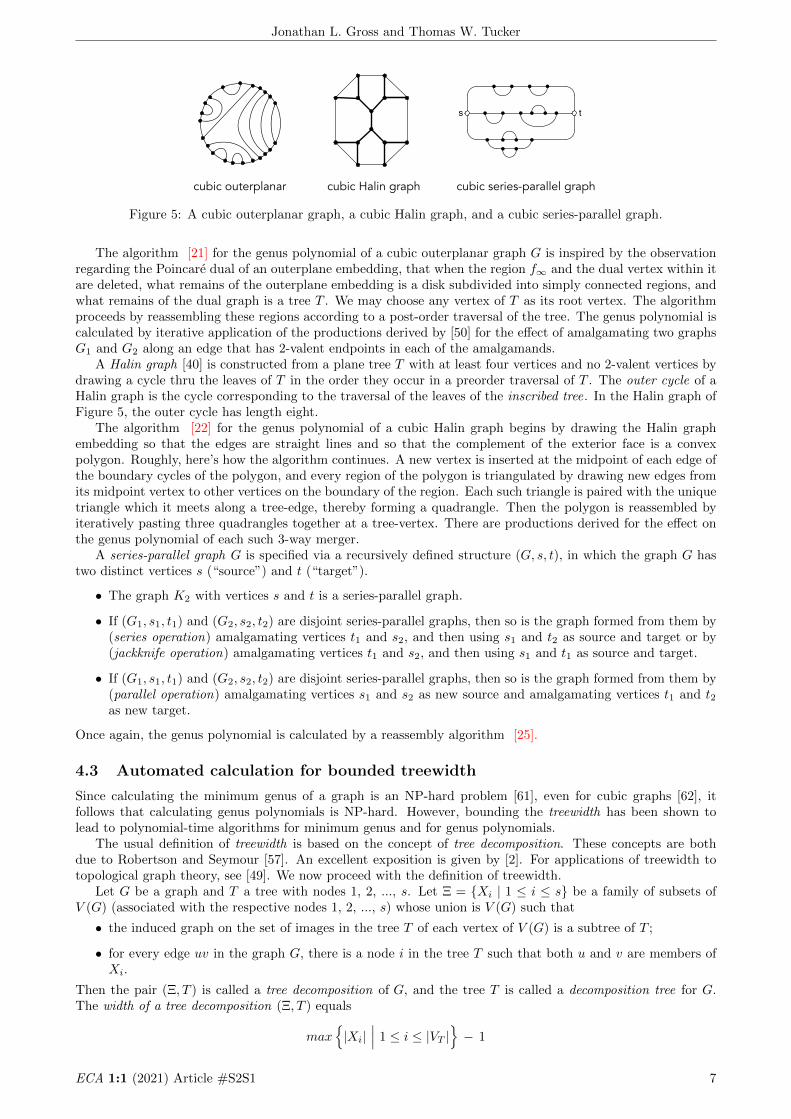
In a non-linear family of known genus distribution of the second kind, the graphs are of low maximum valenceand low treewidth. Three such families, all planar, are illustrated in Figure 5. Rather than a closed formula ora recursion for their genus distributions, we have quadratic-time algorithms.

An outerplanar graph is a graph G that has an embedding in the sphere S0, in which the boundary-walk ofsome face that we will call f∞ contains every vertex of G. Then f∞ is called the exterior face, and the fixedembedding represented is called an outerplane embedding .



s t

cubic outerplanar cubic series-parallel graphcubic Halin graph

Figure 5: A cubic outerplanar graph, a cubic Halin graph, and a cubic series-parallel graph.

The algorithm [21] for the genus polynomial of a cubic outerplanar graph G is inspired by the observationregarding the Poincare dual of an outerplane embedding, that when the region f∞ and the dual vertex within itare deleted, what remains of the outerplane embedding is a disk subdivided into simply connected regions, andwhat remains of the dual graph is a tree T . We may choose any vertex of T as its root vertex. The algorithmproceeds by reassembling these regions according to a post-order traversal of the tree. The genus polynomial iscalculated by iterative application of the productions derived by [50] for the effect of amalgamating two graphsG1 and G2 along an edge that has 2-valent endpoints in each of the amalgamands.

A Halin graph [40] is constructed from a plane tree T with at least four vertices and no 2-valent vertices bydrawing a cycle thru the leaves of T in the order they occur in a preorder traversal of T . The outer cycle of aHalin graph is the cycle corresponding to the traversal of the leaves of the inscribed tree. In the Halin graph ofFigure 5, the outer cycle has length eight.

The algorithm [22] for the genus polynomial of a cubic Halin graph begins by drawing the Halin graphembedding so that the edges are straight lines and so that the complement of the exterior face is a convexpolygon. Roughly, here’s how the algorithm continues. A new vertex is inserted at the midpoint of each edge ofthe boundary cycles of the polygon, and every region of the polygon is triangulated by drawing new edges fromits midpoint vertex to other vertices on the boundary of the region. Each such triangle is paired with the uniquetriangle which it meets along a tree-edge, thereby forming a quadrangle. Then the polygon is reassembled byiteratively pasting three quadrangles together at a tree-vertex. There are productions derived for the effect onthe genus polynomial of each such 3-way merger.

A series-parallel graph G is specified via a recursively defined structure (G, s, t), in which the graph G hastwo distinct vertices s (“source”) and t (“target”).

• The graph K2 with vertices s and t is a series-parallel graph.

• If (G1, s1, t1) and (G2, s2, t2) are disjoint series-parallel graphs, then so is the graph formed from them by(series operation) amalgamating vertices t1 and s2, and then using s1 and t2 as source and target or by(jackknife operation) amalgamating vertices t1 and s2, and then using s1 and t1 as source and target.

• If (G1, s1, t1) and (G2, s2, t2) are disjoint series-parallel graphs, then so is the graph formed from them by(parallel operation) amalgamating vertices s1 and s2 as new source and amalgamating vertices t1 and t2as new target.

Once again, the genus polynomial is calculated by a reassembly algorithm [25].

4.3 Automated calculation for bounded treewidth

Since calculating the minimum genus of a graph is an NP-hard problem [61], even for cubic graphs [62], itfollows that calculating genus polynomials is NP-hard. However, bounding the treewidth has been shown tolead to polynomial-time algorithms for minimum genus and for genus polynomials.

The usual definition of treewidth is based on the concept of tree decomposition. These concepts are bothdue to Robertson and Seymour [57]. An excellent exposition is given by [2]. For applications of treewidth totopological graph theory, see [49]. We now proceed with the definition of treewidth.

Let G be a graph and T a tree with nodes 1, 2, ..., s. Let Ξ = {Xi | 1 ≤ i ≤ s} be a family of subsets ofV (G) (associated with the respective nodes 1, 2, ..., s) whose union is V (G) such that

• the induced graph on the set of images in the tree T of each vertex of V (G) is a subtree of T ;

• for every edge uv in the graph G, there is a node i in the tree T such that both u and v are members ofXi.

Then the pair (Ξ, T ) is called a tree decomposition of G, and the tree T is called a decomposition tree for G.The width of a tree decomposition (Ξ, T ) equals

max{|Xi|

∣∣∣ 1 ≤ i ≤ |VT |}− 1



The treewidth of a graph G is the smallest k such that G has a tree decomposition of width k.For graphs of fixed treewidth and bounded valence, a quadratic-time algorithm is given by [23]. A linear-time

algorithm for the minimum genus of a graph of bounded treewidth is given by [44]. Describing the recursivestep (of adding a copy of the iterated subgraph H) in the construction of the graphs in a linear sequence by theaddition of a set of paths led to an algorithm [26] for automated calculation of the production matrix whoseexecution time is proportional to the square of the number of embedding types.

4.4 Digraph embeddings

An Eulerian digraph is a digraph that has a directed Eulerian circuit that traverses every edge, or equivalently,such that at every vertex, the in-valence and the out-valence are equal.

A cellular embedding of an Eulerian digraph D into a closed surface is said to be a directed embedding if theboundary of each face is a directed closed walk in D. The directed genus polynomial of an Eulerian digraph Dis the polynomial

ΓD(x) =∑h≥0

gh(D)xh

where gh(D) is the number of directed embeddings into the orientable surface Sh of genus h, for h = 0, 1, . . .. The sequence {gh(D)|h ≥ 0}, which is called the directed genus distribution of the digraph D, is known forvery few classes of graphs, compared to the genus distribution of a graph.

Some fundamental results were established by [3]. They include an interpolation theorem, that if there aredirected embeddings of the digraph D in the surfaces Sp and Sq and if p ≤ r ≤ q, then there is a directedembedding of D in Sr. They also show that the gap between the minimum directed genus and the maximumdirected genus of a digraph can be arbitrarily large. Obstructions to planarity were derived by [4]. The directedgenus of the deBruijn graph was obtained by [39].

5. Log-concavity and other possible attributes

A polynomial a0 + a1z + a2z2 + · · ·+ anz

n is said to be log-concave if the inequality

aj−1aj+1 ≤ a2j

holds for 1 ≤ j ≤ n − 1. The following conjecture [36], which has been affirmed for many graphs, is known asthe Log-Concavity Conjecture for Genus Distributions (or by the initials LCGD) is now over 30 years old:

Conjecture 5.1 (LCGD). Every graph has a log-concave genus distribution.

An easily derived variant definition of the log-concavity of a sequence is that the successive ratios of con-secutive elements of the sequence are non-increasing. Proof that the genus polynomials for ladders are log-concave [19] was obtained by applying this variant to a closed form for the coefficients of the genus polynomial.Proof that the genus polynomials for bouquets are log-concave [36] follows inductively from the definition andthe recurrence (8).

A well-known theorem of Newton asserts that if the coefficents of a polynomial are non-negative and allthe roots are real, then the polynomial is log-concave. It is proved by [59] that the genus polynomials derivedin [19] and [36] are real-rooted and then conjectured, after examination of a few more genus polynomials, thatall genus polynomials are real-rooted. However, a counterexample was found by [13].

Whereas the product p(z)q(z) of two log-concave polynomials p(z) and q(z) is log-concave, it is easy toconstruct examples in which the sum p(z) + q(z) is not log-concave. To expand the range of methods ofestablishing the log-concavity of genus polynomials, relations called synchronicity and ratio-dominance wereintroduced by [33] as an aid to proving the log-concavity of linear combinations that correspond to somefrequently used graph operations.

Two non-negative sequences A and B are said to be synchronized , denoted by A ∼ B, if both are log-concaveand if they satisfy the inequalities

aj−1bj+1 ≤ ajbj and aj+1bj−1 ≤ ajbj for all j.

The following theorem of [33] is fundamental.

Theorem 5.1. Let A and B be synchronized sequences, and let u, v > 0. Then the sequence uA + vB islog-concave.



Let A = (aj) and B = (bj) both be non-negative synchronized sequences. Then B is said to be ratio-dominant over A, denoted by B & A or A . B, if

aj+1bj ≤ ajbj+1 for all j.

That the convolution operator ∗ preserves log-concavity is well-known. The following theorem is used inproofs of log-concavity of the genus polynomials of graphs that are constructed by amalgamating two differentgraphs.

Theorem 5.2 ( [33]). Let A,B,C,D be four non-negative log-concave sequences without internal zeros, suchthat A . B and C . D. Then the convolution sequences A ∗D and B ∗ C are synchronized.

The directed genus distribution of a 4-regular outerplanar digraph was derived and proved by [8] to belog-concave. Indeed, the corresponding genus polynomial is real-rooted.

6. Monodromy and Ribbon graphs

The flags of an embedded graph G are the faces of a barycentric subdivision of the embedding. We observethat every flag is 3-sided and that there are four flags incident on every edge of G. The canonical flag-labelingconvention has a couple of uncomplicated rules, introduced in [31], for labeling the edges and flags of anembedded graph G with n edges. These rules simplify the algorithms for computations.

1. Label the edges of G by the integers 1, 2, . . . , n.

2. Label the flags incident on edge j by the integers 4j–3, 4j–2, 4j–1, 4j, so that flag 4j–2 is on the sameside of edge j as flag 4j–3 and so that flag 4j lies immediately opposite flag 4j–3 on the other side of edgej.

Figure 6 illustrates this configuration. Artifacts of the barycentric subdivision are shown with broken straight-edges and hollow vertices.

v

edge j

4j-3 4j-2

4j-14j

Figure 6: The canonical labeling of the four flags incident on edge j.

We now proceed with descriptions of the three paradigms mentioned in Section 1 for specifying a graphembedding: rotation systems, monodromy, and ribbon graphs.

6.1 Monodromy

Jones and Singerman [43] showed how a graph embedding could be specified by a set of three fixed-point-freeinvolutions {r0, r1, r2}, called the monodromy of the embedding , on the set of flags. The group that theygenerate is called the monodromy group. Using the canonical labeling of the flags, the involutions r0 and r2 forany embedded graph with n edges are always the following:

r0 = (1 2)(3 4)(5 6)(7 8) · · · (4n–3 4n–2)(4n–1 4n) (9)

r2 = (1 4)(2 3)(5 8)(6 7) · · · (4n–3 4n)(4n–2 4n–1). (10)

To describe the involution r1, we observe that the flags of any graph embedding are partitionable into cycles inwhich two consecutive flags lie in the same face of the embedding, with two flags in each corner of every face ofthe corresponding map. We define r1 as the full involution that transposes every flag with the other flag in thesame corner of the map. It should be clear that if we visualize each transposition in any of these involutions asa rule for pasting two flags together, we can reconstruct the embedding from its monodromy.

Proposition 6.1. Let {r0, r1, r2} be the monodromy of a graph embedding, and let λ = r0r2. Then thePoincare dual embedding has the monodromy

{r∗0 = r0λ, r∗1 = r1, r∗2 = r2λ}. (11)

We observe that under the canonical labeling convention, we have

λ = (1 3)(2 4)(5 7)(6 8) · · · (4n–3 4n–1)(4n–2 4n). (12)



6.2 Ribbon graphs

Formally, a ribbon graph, as defined by [53], is equivalent to a band decomposition as defined by [37], that is,a collection of disks and bands assembled as in Figure 7. Topologically, it is a surface with holes. The graphthat it specifies is obtained by envisioning a vertex in the interior of each disk and an edge traversing eachband, which joins the vertices in the disks at the opposite ends of the band. Any such ribbon graph has animplicit imbedding that is obtained by attaching the boundary of a disk to each of the boundary components. Indiscussion of ribbon graphs, including in this paper, the same phrase “ribbon graph” may refer to the implicitgraph embedding.

Figure 7: A ribbon graph whose embedding surface is the projective plane.

7. Partial dualities

In this section, we define and discuss Petrie duality and Wilson duality. We recall from Subsection 6.1 that thePoincare duality operator is denoted by ∗. Propositions 6.1 and 7.1 give the transformation on the monodromyof a ribbon graph G corresponding to ∗-duality and partial ∗-duality, respectively. The Petrie and Wilsonduality operators are denoted by × and ∗×∗, respectively.

Chmutov [16] invented a way to define the Poincare partial-dual of a ribbon graph G, in which one candualize any edge-subset A of G, in terms of a topological modification of the ribbon graph G. Since we denotethe Poincare dual of G by G∗, we denote the partial-dual on A by G∗|A . Although the full Poincare dual has thesame surface as the primal graph, partial-dualizing can change the surface type. For instance, partial-dualizingon one edge of a 2-cycle C2 in the sphere S0 results in an embedding of the bouquet B2 (a single vertex withtwo loops) in the torus S1. This partial-dual construction was extensively developed by [18].

To define G∗|A in terms of permutation algebra, we begin with the definition

λ|A =∏j∈A

(4j–3 4j–1)(4j–2 4j) (13)

of λ|A as the restriction of λ to the edge-set A. This facilitates the computationally tractable definition of thepartial dual of the embedded graph with monodromy {r0, r1, r2}, as the embedded graph with monodromy

{r∗|A0 = r0λ|A, r∗|A1 = r1, r∗|A2 = r2λ|A}. (14)

Proposition 7.1. The monodromy transformation given by (14) is equivalent to Chmutov’s geometric con-struction of a partial-∗ dual.

The partial-dual genus polynomial ∂Γ∗G(z), for the Poincare dual, as introduced by [30], is given by

∂Γ ∗G(z) =

∑A⊂E(G)

zγ(G∗|A). (15)

The Petrie dual was originally conceived as a geometric construction. Its generalization to an operation onembedded graphs, and also the corresponding partial dual, are easily expressed in terms of a ribbon graph. ThePetrie duality operator is indicated by ×.

• The Petrie dual of a ribbon graph G is the ribbon graph G× obtained by giving every ribbon a half-twist.Of course, the Petrie dual of an orientable ribbon graph may be non-orientable.

• The partial Petrie dual of a ribbon graph G on an edge set A is the ribbon graph G×|A obtained by givinga half-twist to each ribbon whose corresponding edge lies in the edge-set A.

Proposition 7.2. Let {r0, r1, r2} be the monodromy of a graph embedding, and let λ = r0r2. Then the Petriedual embedding has the monodromy

{r×0 = r0r2, r×1 = r1, r×2 = r2}. (16)

ECA 1:1 (2021) Article #S2S1 10


Analogous to the definition (13) of λ|A, we now define

r2|A =∏j∈A

(4j–3 4j)(4j–2 4j–1). (17)

Proposition 7.3. Let {r0, r1, r2} be the monodromy of a graph embedding. Then the partial Petrie dual onthe edge-subset A has the monodromy

{r×|A0 = r0r2|A, r×|A1 = r1, r

×|A2 = r2}. (18)

The Wilson dual is the iterated composition ∗×∗ of Poincare and Petrie duals.

Proposition 7.4. Let {r0, r1, r2} be the monodromy of a graph embedding, and let λ = r0r2. Then theWilson dual embedding has the monodromy

{r∗×∗0 = r0, r∗×∗1 = r1, r∗×∗2 s = r2r0}. (19)

Analogous to the definitions (13) and (17), we now define

r0|A =∏j∈A

(4j–3 4j − 2)(4j–1 4j). (20)

Proposition 7.5. Let {r0, r1, r2} be the monodromy of a graph embedding. Then the partial Wilson dual onthe edge-subset A has the monodromy

{r∗×∗|A0 = r0r2|A, r∗×∗|A1 = r1, r

∗×∗|A2 = r2}. (21)

The following theorem indicates a close relationship between the partial-∗×∗ and partial-× polynomials:

Theorem 7.1. Let G be a ribbon graph. Then

∂E∗×∗G (z) = ∂E×G∗(z). (22)

8. Some partial-duality polynomial formulas

Partial-dual polynomials formulas for a number of sequences of ribbon graphs were derived in [31]. Four ofthese sequences are represented by graphic images in Figure 8. These four sequences and two related sequences,both quite easily visualized, are listed immediately below the figure.

e1 e1

e1

e1e1

e5

e2e2

e2

e2

e2

e3e3

e3

e3

e4

e4

en

en

en

(2) Dn S0 >

(5) Bn N1 > (6 odd) B3 S1 >

a

b

c

d

a

a

a

a a

b

b

b

c

c

c

d

>(3 odd) D5 S2

e1

e1

e5

e2

e2

e3

e3

e4

e4

e6

a

b

c

d

a

b

c

d

>(3 even) D6 S2

e1

e1e1

e2

e2

e2

e2

e3e3

e3e3

e4

e4

a

b

c

d

a

b

c

d

>(6 even) B4 S2

e1

Figure 8: Representatives of some embedding sequences with known partial-dual polynomial formulas.

1. Cn → S0 is the n-cycle Cn in the sphere S0.

ECA 1:1 (2021) Article #S2S1 11


2. Dn → S0 is the dipole Dn in the sphere.

3. Dn → Sp(n)/2, where p(n) =

{n− 1 if n odd

n− 2 if n even

is the dipole Dn is the orientable surface of genus p(n)/2.

4. Cn → N1 is the n cycle in the projective plane N1.

5. Bn → N1 is the n-bouquet in the projective plane.

6. Bn → Sq(n)/2, where q(n) =

{n− 1 if n odd

n if n even

is the bouquet Bn in the orientable surface of genus q(n)/2.

Table 2 gives the formulas for the partial-∗,×, and ∗ ×∗ polynomials for each of the first six sequences. Forconvenience, we refer to columns 3, 4, and 5 of that table according to the duality operator ∗,×, ∗×∗ to whichthey correspond. We refer to a row according to its entry in column 1. Thus, the notation (2×) in row (1),column ∗×∗ indicates (as we explain below) that the formula for the partial-∗×∗ polynomials for the ribbongraph sequence Cn → S0 equals the formula in row (2), column ×, that is, the same as the formula for thepartial-× polynomials for the ribbon graph sequence Dn → S0.

Table 2: Partial-∗,×, ∗×∗ polynomial formulas for six families of ribbon graphs. We define p(n) = n–1 forodd n and p(n) = n–2 for even n. We define q(n) = n–1 for odd n and q(n) = n for even n.

row embedding ∂E∗(z) ∂E

×(z) ∂E

∗×∗(z)

(1) Cn → S0 2 + (2n − 2)z2 2n−1(1 + z) (2×)

(2) Dn → S0q (1 + z)n − zn + zp(n) (1×)

(3 oddn) Dn → S(n−1)/2 2nzn−1 q (5×)

(3 evenn) Dn → S(n−2)/2 2n−1(zn−2 + zn) q (2×)

(4) Cn → N1 2z + (2n − 2)z2 (1×) (4×)=(1×)

(5) Bn → N1q z(1 + z)n − zn+1 + zq(n) (4×)=(1×)

(6 oddn) Bn → S(n−1)/2 (3 oddn ∗) q (2×)

(6 evenn) Bn → Sn/2 (3 evenn ∗) q (5×)

As demonstrated in [31], these sequences are interrelated according to two principles:

(a) For each of the dualities • = ∗,×, ∗×∗, a ribbon graph and any of its partial-• duals have the samepartial-• polynomial.

(b) For any ribbon graph G, we have ∂E∗×∗G (z) = ∂E×G∗(z). This is Theorem 7.1.

For instance, the ribbon graph (2) Dn → S0 is the full ∗-dual of (1) Cn → S0, so by principle (a), they havethe same partial-∗ polynomial. Moreover, since (2) Dn → S0 is the full ∗-dual of (1) Cn → S0, it follows fromprinciple (b) that the partial-∗×∗ polynomial of (1) Cn → S0 equals the partial-× polynomial of (2) Dn → S0.

8.1 Ladders

In this subsection, we present partial-∗, ×, and ∗×∗ polynomials for the ladder graphs.

Theorem 8.1. [30] Let pn(z) = ∂Γ∗Ln(z) and qn(z) = ∂Γ∗Qn

(z). Then the resulting polynomials satisfy thesimultaneous recurrence:

pn+1(z) = 6zpn(z) + qn(z) (23)

qn+1(z) = (6z + 4z2)pn(z) + (1 + 2z)qn(z) (24)

Theorem 8.2. [30] The polynomial ∂Γ∗Ln(z) for the ladders is given by

∂Γ∗Ln(z) = 2(

√8z)n−1

(1 + 6z + z2

2√

2zUn−2(t)− Un−3(t)

),

where t = 1+8z4√2z

and Um(t) is the mth Chebyshev polynomial of the second kind.

ECA 1:1 (2021) Article #S2S1 12


Theorem 8.3. [31] The ladder graph Ln (embedded in the 2-sphere S0, as shown in Figure 9) has the partial-×polynomial recursion

∂E×L0(z) = 2

∂E×L1(z) = 8 + 8z

∂E×Ln(z) = (2 + 4z)∂E×Ln−1

(z) + (16z2)∂E×Ln−2(z) for n ≥ 2.

with the closed form

∂E×Ln(z) = 2(4iz)n

(1 + z

izUn−1

(1 + 2z

4iz

)− Un−2

(1 + 2z

4iz

)), (25)

where i2 = −1 and Un(t) is the nth Chebyshev polynomial. The polynomial ∂E×Ln(z) is log-concave.

e5e4e3e2e1

Figure 9: Embedding of the ladder L5 in the sphere S0.

Lemma 8.1. [31] Let e be any edge of a ribbon graph G. Let H be obtained from G by adding an edgeparallel to e and then trisecting it by adding two vertices of valence two. Then

∂E∗×∗H (z) = (1 + 3z + 4z2)∂E∗×∗G (z).

Theorem 8.4. [31] The ladder Ln has the partial-∗×∗ polynomial

∂E∗×∗Ln= (1 + z)(1 + 3z + 4z2)n.

Proof. The ladder L0 consists of a single edge, so ∂E∗×∗L0= 1 + z. Since Ln is obtained from Ln−1 by adding a

trisected parallel edge, this follows from Lemma 8.1.

8.2 A family of series-parallel graphs

The family of restricted series-parallel ribbon graphs, abbreviated RSPG, is recursively constructed, beginningwith the trivial ribbon graph K1. It is closed under the following operations: (1) adding a parallel edge or atrisected parallel edge; (2) ribbon-joins; (3) bar-amalgamations. All trees and ladders are in RSPG, but so areribbon graphs like the one shown in Figure 10.

Figure 10: An RSPG graph that is not a tree or a ladder.

Theorem 8.5. [31] Let G be any ribbon graph in RSPG. Then

∂E∗×∗G (z) = ∂E×G∗(z) = 2k(1 + z)m(1 + 3z + 4z2)n,

where k is the number of parallel edges, m is the number of bar-amalgamations, and n is the number of trisectedparallel edges used in the construction of G.

9. Some research problems

We are concerned here with the derivation of methods for calculating genus polynomials and partial-dualitypolynomials for a number of graphs and embeddings of general interest. An attractive common feature of theexamples we present in this section is that each of them has a plane embedding or a plane projection withcircular symmetry.

ECA 1:1 (2021) Article #S2S1 13


9.1 Anti-prisms

The n-anti-prism is the graph formed from two concentric n-gons so that each vertex of one of the n-gons arejoined to the endpoints of an edge the other n-gon, as illustrated in Figure 11. Each anti-prism graph is the1-skeleton of the Archimedean solid from which its name is taken, in which all of the 3-sided faces are equilateraltriangles.

4-antiprism 5-antiprism

Figure 11: Two anti-prism graphs.

Problem 9.1. Derive the genus polynomials for the sequence of anti-prism graphs.

Problem 9.2. Derive the partial-dual polynomial of the spherically embedded anti-prism graphs for any or allof the dualities ∗,×, ∗×∗.

9.2 Truncated pyramid

The truncated n-pyramid is the 1-skeleton of the solid formed by truncating all the corners of the pyramid withan n-gon as its base. (In some contexts other than graph theory, the apex of the pyramid would be truncated,but not the corners of its base.)

truncated 3-pyramid truncated 4-pyramid

Figure 12: Two truncated-pyramid graphs.

Problem 9.3. Derive the genus polynomials for the sequence of truncated-pyramid graphs.

Problem 9.4. Derive the partial-dual polynomials of the spherically embedded truncated-pyramid graphs forany or all of the dualities ∗,×, ∗×∗.

9.3 Ring-like ladder graphs

Problem 9.5. Derive the partial-dual polynomials of the spherically embedded ladder graphs for any or all ofthe dualities ∗,×, ∗×∗.

Problem 9.6. Derive the partial-dual polynomials of the Mobius ladder graphs embedded in the projectiveplane N1 for any or all of the dualities ∗,×, ∗×∗.

9.4 Circulant graphs

A circulant graph circ(n;X) is defined for a positive integer n and a subset X of the integers 1, 2, . . . bn/2c,called the connections.

• The vertex set is Zn, the integers modulo n.

• There is an edge joining the vertices i and j if and only if the number |j − i is one of the connections.

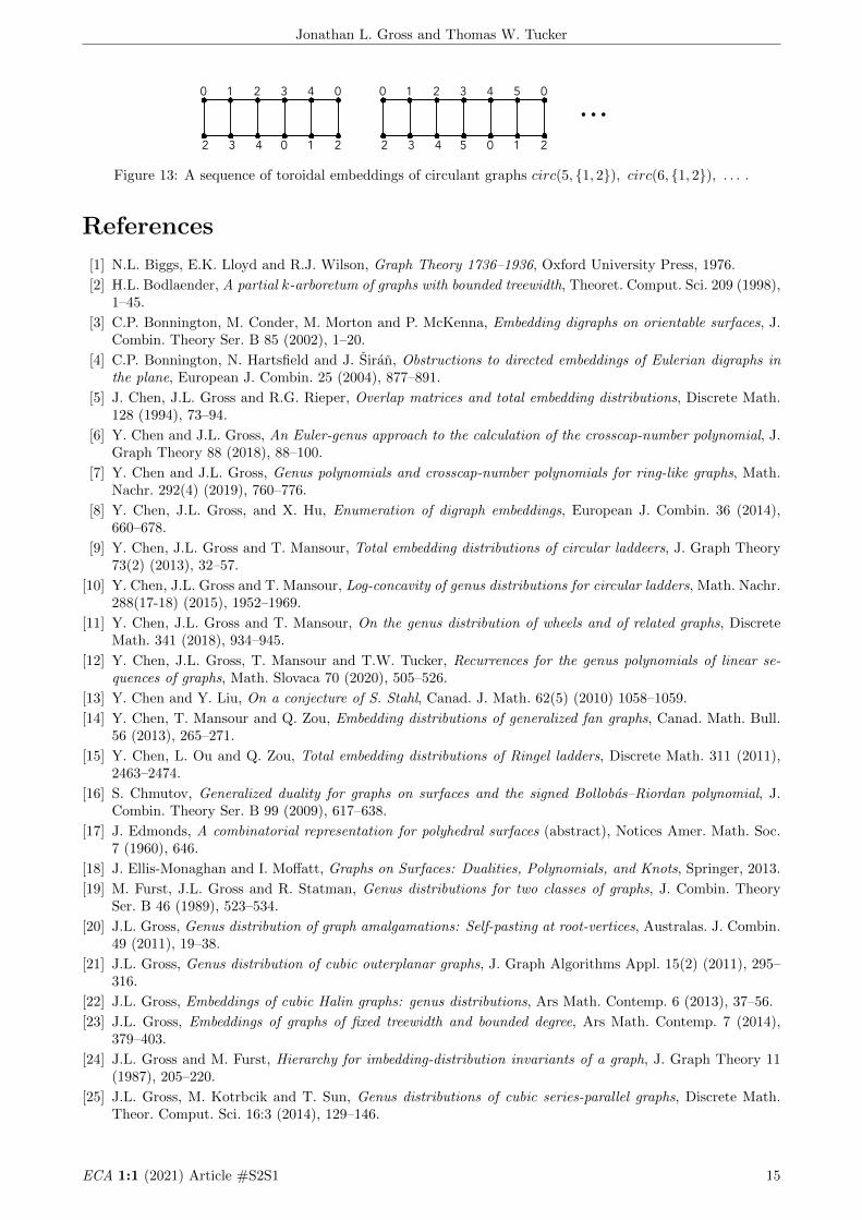
For instance, the graph circ(5, {1, 2}) is isomorphic to the Kuratowski graph K5 (and not to the cicular ladderCL5). Corresponding to the sequence of circulant graphs circ(n, {1, 2}) for n ≥ 5, there is a sequence of toroidalembeddings, as shown in Figure 13.

Problem 9.7. Derive the partial-∗,×, ∗×∗ polynomials for the toroidally embedded circulant graphs circ(n, {1, 2})for n ≥ 5.

ECA 1:1 (2021) Article #S2S1 14


0 0432

0432

1

21

0 05

5

432

0432

1

21

...

Figure 13: A sequence of toroidal embeddings of circulant graphs circ(5, {1, 2}), circ(6, {1, 2}), . . . .

References

[1] N.L. Biggs, E.K. Lloyd and R.J. Wilson, Graph Theory 1736–1936, Oxford University Press, 1976.

[2] H.L. Bodlaender, A partial k-arboretum of graphs with bounded treewidth, Theoret. Comput. Sci. 209 (1998),1–45.

[3] C.P. Bonnington, M. Conder, M. Morton and P. McKenna, Embedding digraphs on orientable surfaces, J.Combin. Theory Ser. B 85 (2002), 1–20.

[4] C.P. Bonnington, N. Hartsfield and J. Siran, Obstructions to directed embeddings of Eulerian digraphs inthe plane, European J. Combin. 25 (2004), 877–891.

[5] J. Chen, J.L. Gross and R.G. Rieper, Overlap matrices and total embedding distributions, Discrete Math.128 (1994), 73–94.

[6] Y. Chen and J.L. Gross, An Euler-genus approach to the calculation of the crosscap-number polynomial, J.Graph Theory 88 (2018), 88–100.

[7] Y. Chen and J.L. Gross, Genus polynomials and crosscap-number polynomials for ring-like graphs, Math.Nachr. 292(4) (2019), 760–776.

[8] Y. Chen, J.L. Gross, and X. Hu, Enumeration of digraph embeddings, European J. Combin. 36 (2014),660–678.

[9] Y. Chen, J.L. Gross and T. Mansour, Total embedding distributions of circular laddeers, J. Graph Theory73(2) (2013), 32–57.

[10] Y. Chen, J.L. Gross and T. Mansour, Log-concavity of genus distributions for circular ladders, Math. Nachr.288(17-18) (2015), 1952–1969.

[11] Y. Chen, J.L. Gross and T. Mansour, On the genus distribution of wheels and of related graphs, DiscreteMath. 341 (2018), 934–945.

[12] Y. Chen, J.L. Gross, T. Mansour and T.W. Tucker, Recurrences for the genus polynomials of linear se-quences of graphs, Math. Slovaca 70 (2020), 505–526.

[13] Y. Chen and Y. Liu, On a conjecture of S. Stahl, Canad. J. Math. 62(5) (2010) 1058–1059.

[14] Y. Chen, T. Mansour and Q. Zou, Embedding distributions of generalized fan graphs, Canad. Math. Bull.56 (2013), 265–271.

[15] Y. Chen, L. Ou and Q. Zou, Total embedding distributions of Ringel ladders, Discrete Math. 311 (2011),2463–2474.

[16] S. Chmutov, Generalized duality for graphs on surfaces and the signed Bollobas–Riordan polynomial, J.Combin. Theory Ser. B 99 (2009), 617–638.

[17] J. Edmonds, A combinatorial representation for polyhedral surfaces (abstract), Notices Amer. Math. Soc.7 (1960), 646.

[18] J. Ellis-Monaghan and I. Moffatt, Graphs on Surfaces: Dualities, Polynomials, and Knots, Springer, 2013.

[19] M. Furst, J.L. Gross and R. Statman, Genus distributions for two classes of graphs, J. Combin. TheorySer. B 46 (1989), 523–534.

[20] J.L. Gross, Genus distribution of graph amalgamations: Self-pasting at root-vertices, Australas. J. Combin.49 (2011), 19–38.

[21] J.L. Gross, Genus distribution of cubic outerplanar graphs, J. Graph Algorithms Appl. 15(2) (2011), 295–316.

[22] J.L. Gross, Embeddings of cubic Halin graphs: genus distributions, Ars Math. Contemp. 6 (2013), 37–56.

[23] J.L. Gross, Embeddings of graphs of fixed treewidth and bounded degree, Ars Math. Contemp. 7 (2014),379–403.

[24] J.L. Gross and M. Furst, Hierarchy for imbedding-distribution invariants of a graph, J. Graph Theory 11(1987), 205–220.

[25] J.L. Gross, M. Kotrbcik and T. Sun, Genus distributions of cubic series-parallel graphs, Discrete Math.Theor. Comput. Sci. 16:3 (2014), 129–146.

ECA 1:1 (2021) Article #S2S1 15


[26] J.L. Gross, I.F. Khan, T. Mansour and T.W. Tucker, Calculating genus polynomials via string operationsand matrices, Ars Math. Contemp. 15 (2018), 267–295.

[27] J.L. Gross, I.F. Khan and M.I. Poshni, Genus distributions for iterated claws, Electron. J. Combin. 21(1)(2014), #P1.12.

[28] J.L. Gross, I.F. Khan and M.I. Poshni, Genus distribution of graph amalgamations: Pasting at root-vertices,Ars Combin. 94 (2010), 33–53

[29] J.L. Gross, T. Mansour and T.W. Tucker, Valence-partitioned genus polynomials and their application togeneralized dipoles, Australas. J. Combin. 67(2) (2017), 203–221.

[30] J.L. Gross, T. Mansour and T.W. Tucker, Partial duality for ribbon graphs, I: Distributions, European J.Combin. 86 (2020), 103084.

[31] J.L. Gross, T. Mansour and T.W. Tucker, Partial duality for ribbon graphs, II: partial-twuality polynomialsand monodromy computations, manuscript, 2020.

[32] J.L. Gross, T. Mansour and T.W. Tucker, Partial duality for ribbon graphs, III: a Gray code algorithm forenumeration, manuscript, 2020.

[33] J.L. Gross, T. Mansour, T.W. Tucker and D.G.L. Wang, Log-concavity of combinations of sequences andapplications to genus distributions, SIAM J. Discrete Math. 29(2) (2015), 1002–1029.

[34] J.L. Gross, T. Mansour, T.W. Tucker and D.G.L. Wang, Log-concavity of the genus polynomials of Ringelladders, Electron. J. Graph Theory Appl. 3 (2015), 109–126.

[35] J.L. Gross, T. Mansour, T.W. Tucker and D.G.L. Wang, Iterated claws have real-rooted genus polynomials,Ars Math. Contemp. 10 (2016), 255–268.

[36] J.L. Gross, D.P. Robbins and T.W. Tucker, Genus distributions for bouquets of circles, J. Combin. TheorySer. B 47 (1989), 292–306.

[37] J.L. Gross and T.W. Tucker, Topological Graph Theory. Wiley, 1987 (reprinted by Dover, 2001).

[38] W. Gustin, Orientable embedding of Cayley graphs, Bull. Amer. Math. Soc. 69 (1963), 272–275.

[39] A.W. Hales and N. Hartsfield, The directed genus of the de Bruijn graph, Discrete Math. 309 (2009),5259–5263.

[40] R. Halin, Uber simpliziale Zerfallungen beliebiger (endlicher oder unendlicher) Graphen, Math. Ann. 156(1964), 216–225.

[41] L. Heffter, Uber das Problem der Nachbargebiete, Math. Ann. 38 (1891), 477–508.

[42] D.M. Jackson, Counting cycles in permutations by group characters, with an application to a topologicalproblem, Trans. Amer. Math. Soc. 299 (1987), 785–801.

[43] G.A. Jones and D. Singerman, Theory of maps on orientable surfaces, Proc. Lond. Math. Soc. III 37 (1978),273–307.

[44] K. Kawarabayashi, B. Mohar and B. Reed, A simpler linear time algorithm for embedding graphs into anarbitrary surface and the genus of graphs of bounded tree-width, Proc. 49th Ann. Symp. on Foundations ofComput. Sci. (FOCS’08) IEEE (2008), 771–780.

[45] J.H. Kwak and J. Lee, Genus polynomials of dipoles, Kyungpook Math. J. 33 (1993), 115–125.

[46] J.H. Kwak and S.H. Shim, Total embedding distributions for bouquets of circles, Discrete Math. 248 (2002),93–108.

[47] L.A. McGeoch, Algorithms for two graph problems: computing a maximum genus imbedding and the two-server problem, PhD thesis, Carnegie-Mellon Univ., 1987.

[48] B. Mohar, An obstruction to embedding graphs in surfaces, Discrete Math. 78 (1989), 135–142.

[49] B. Mohar and C. Thomassen, Graphs on Surfaces, Johns Hopkins University Press, 2001.

[50] M.I. Poshni, I.F. Khan and J.L. Gross, Genus distribution of edge-amalgamations, Ars Math. Contemp. 3(2010), 69–86.

[51] M.I. Poshni, I.F. Khan and J.L. Gross, Genus distribution of 4-regular outerplanar graphs, Electron. J.Combin. 18 (2011), #P212.

[52] M.I. Poshni, I.F. Khan and J.L. Gross, Genus distribution of graphs under self-edge-amalgamations, ArsMath. Contemp. 5 (2012), 127–248.

[53] N. Reshetikhin and V. Turaev, Ribbon graphs and their invariants derived from quantum groups, Comm.Math. Phys. 127 (1990), 1–26.

[54] R.G. Rieper, The enumeration of graph imbeddings, Ph.D. Dissertation, Western Michigan University, 1990.

[55] G. Ringel and J.W.T. Youngs, Solution of the Heawood map-coloring problem, Proc. Nat. Acad. Sci. USA60 (1968), 438–445.

[56] T. Rivlin, Chebyshev Polynomials. From Approximation Theory to Algebra and Number Theory, JohnWiley, New York, 1990.

ECA 1:1 (2021) Article #S2S1 16


[57] N. Robertson and P.D. Seymour, Graph minors. II, Algorithmic aspects of tree-width, J. Algorithms 7(1986), 309–322.

[58] S. Stahl, Permutation-partition pairs. III. Embedding distributions of linear families of graphs, J. Com-bin. Theory B 52 (1991), 191–218.

[59] S. Stahl, On the zeros of some genus polynomials, Canad. J. Math. 49 (1997), 617–640.

[60] E.H. Tesar, Genus distributions of Ringel ladders, Discrete Math. 216 (2000), 235–252.

[61] C. Thomassen, The graph genus problem is NP-complete, J. Algorithms 10 (1989), 568–576.

[62] C. Thomassen, The genus problem for cubic graphs, J. Combin. Theory Ser. B 69 (1997), 52–58.

[63] T.I. Visentin and S.W. Wieler, On the genus distribution of (p, q, n)-dipoles, Electron. J. Combin. 14 (2007),#R12.

[64] A.T. White, Graphs of Groups on Surfaces, North-Holland, 2001.

[65] D. Zagier, On the distribution of the number of cycles of elements in symmetric groups, Nieuw Arch. Wiskd.13(3) (1995), 489–495.

ECA 1:1 (2021) Article #S2S1 17

enumerating graph embeddings and partial-duals by genus

Documents